statistics-lab™ 为您的留学生涯保驾护航 在代写运筹学operational research方面已经树立了自己的口碑, 保证靠谱, 高质且原创的统计Statistics代写服务。我们的专家在代写运筹学operational research代写方面经验极为丰富，各种代写运筹学operational research相关的作业也就用不着说。

如果你也在 怎样代写运筹学Operations Research 这个学科遇到相关的难题，请随时右上角联系我们的24/7代写客服。运筹学Operations Research（英式英语：operational research），通常简称为OR，是一门研究开发和应用先进的分析方法来改善决策的学科。它有时被认为是数学科学的一个子领域。管理科学一词有时被用作同义词。

运筹学Operations Research采用了其他数学科学的技术，如建模、统计和优化，为复杂的决策问题找到最佳或接近最佳的解决方案。由于强调实际应用，运筹学与许多其他学科有重叠之处，特别是工业工程。运筹学通常关注的是确定一些现实世界目标的极端值：最大（利润、绩效或收益）或最小（损失、风险或成本）。运筹学起源于二战前的军事工作，它的技术已经发展到涉及各种行业的问题。

数学代写|运筹学作业代写operational research代考|ASSUMPTIONS OF LINEAR PROGRAMMING

All the assumptions of linear programming actually are implicit in the model formulation given in Sec. 3.2. However, it is good to highlight these assumptions so you can more easily evaluate how well linear programming applies to any given problem. Furthermore, we still need to see why the OR team for the Wyndor Glass Co. concluded that a linear programming formulation provided a satisfactory representation of the problem.
Proportionality
Proportionality is an assumption about both the objective function and the functional constraints, as summarized below.
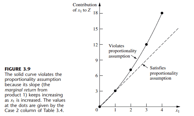
Proportionality assumption: The contribution of each activity to the value of the objective function $Z$ is proportional to the level of the activity $x_j$, as represented by the $c_j x_j$ term in the objective function. Similarly, the contribution of each activity to the left-hand side of each functional constraint is proportional to the level of the activity $x_j$, as represented by the $a_{i j} x_j$ term in the constraint.

Consequently, this assumption rules out any exponent other than 1 for any variable in any term of any function (whether the objective function or the function on the left-hand side of a functional constraint) in a linear programming model. ${ }^1$
To illustrate this assumption, consider the first term $\left(3 x_1\right)$ in the objective function $\left(Z=3 x_1+5 x_2\right.$ ) for the Wyndor Glass Co. problem. This term represents the profit generated per week (in thousands of dollars) by producing product 1 at the rate of $x_1$ batches per week. The proportionality satisfied column of Table 3.4 shows the case that was assumed in Sec. 3.1, namely, that this profit is indeed proportional to $x_1$ so that $3 x_1$ is the appropriate term for the objective function. By contrast, the next three columns show different hypothetical cases where the proportionality assumption would be violated.

数学代写|运筹学作业代写operational research代考|Additivity

Although the proportionality assumption rules out exponents other than 1 , it does not prohibit cross-product terms (terms involving the product of two or more variables). The additivity assumption does rule out this latter possibility, as summarized below.
Additivity assumption: Every function in a linear programming model (whether the objective function or the function on the left-hand side of a functional constraint) is the sum of the individual contributions of the respective activities.
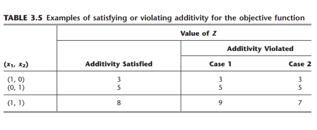
To make this definition more concrete and clarify why we need to worry about this assumption, let us look at some examples. Table 3.5 shows some possible cases for the objective function for the Wyndor Glass Co. problem. In each case, the individual contributions from the products are just as assumed in Sec. 3.1 , namely, $3 x_1$ for product 1 and $5 x_2$ for product 2. The difference lies in the last row, which gives the function value for $Z$ when the two products are produced jointly. The additivity satisfied column shows the case where this function value is obtained simply by adding the first two rows $(3+5=8)$, so that $Z=3 x_1+5 x_2$ as previously assumed. By contrast, the next two columns show hypothetical cases where the additivity assumption would be violated (but not the proportionality assumption).

Referring to the Case 1 column of Table 3.5 , this case corresponds to an objective function of $Z=3 x_1+5 x_2+x_1 x_2$, so that $Z=3+5+1=9$ for $\left(x_1, x_2\right)=(1,1)$, thereby violating the additivity assumption that $Z=3+5$. (The proportionality assumption still is satisfied since after the value of one variable is fixed, the increment in $Z$ from the other variable is proportional to the value of that variable.) This case would arise if the two products were complementary in some way that increases profit. For example, suppose that a major advertising campaign would be required to market either new product produced by itself, but that the same single campaign can effectively promote both products if the decision is made to produce both. Because a major cost is saved for the second product, their joint profit is somewhat more than the sum of their individual profits when each is produced by itself.

Case 2 in Table 3.5 also violates the additivity assumption because of the extra term in the corresponding objective function, $Z=3 x_1+5 x_2-x_1 x_2$, so that $Z=3+5-1=7$ for $\left(x_1, x_2\right)=(1,1)$. As the reverse of the first case, Case 2 would arise if the two products were competitive in some way that decreased their joint profit. For example, suppose that both products need to use the same machinery and equipment. If either product were produced by itself, this machinery and equipment would be dedicated to this one use. However, producing both products would require switching the production processes back and forth, with substantial time and cost involved in temporarily shutting down the production of one product and setting up for the other. Because of this major extra cost, their joint profit is somewhat less than the sum of their individual profits when each is produced by itself.

运筹学代考

数学代写|运筹学作业代写operational research代考|ASSUMPTIONS OF LINEAR PROGRAMMING

线性规划的所有假设实际上都隐含在3.2节给出的模型公式中。然而，强调这些假设是很好的，这样您就可以更容易地评估线性规划对任何给定问题的应用效果。此外，我们还需要了解为什么温多尔玻璃公司的OR团队得出结论，线性规划公式提供了一个令人满意的问题表示。
比例
比例性是关于目标函数和功能约束的假设，如下所述。
比例假设:每个活动对目标函数$Z$值的贡献与活动$x_j$的水平成正比，由目标函数中的$c_j x_j$项表示。类似地，每个活动对每个功能约束左侧的贡献与活动$x_j$的级别成正比，由约束中的$a_{i j} x_j$项表示。

因此，该假设排除了线性规划模型中任何函数(无论是目标函数还是函数约束左侧的函数)的任何项中的任何变量的除1以外的任何指数。${} ^ 1美元
为了说明这个假设，考虑目标函数$\left(Z= 3x_1 + 5x_2 \right)中的第一项$\left(3x_1 \right)$。windor Glass Co.的问题。这一项表示以每周生产$x_1$批的速度生产产品1每周产生的利润(以千美元为单位)。表3.4的比例满足列显示了3.1节中假设的情况，即该利润确实与$x_1$成正比，因此$ 3x_1 $是目标函数的适当项。相比之下，接下来的三列显示了违反比例假设的不同假设情况。

数学代写|运筹学作业代写operational research代考|Additivity

虽然比例假设排除了除1以外的指数，但它并不禁止交叉乘积项(涉及两个或多个变量乘积的项)。可加性假设排除了后一种可能性，总结如下。
可加性假设:线性规划模型中的每个函数(无论是目标函数还是功能约束左侧的函数)都是各自活动的个人贡献的总和。
为了使这个定义更具体，并澄清为什么我们需要担心这个假设，让我们看一些例子。表3.5显示了温多玻璃公司问题的目标函数的一些可能情况。在每种情况下，每个产品的贡献就像3.1节中假设的那样，即产品1的贡献为$ 3x_1 $，产品2的贡献为$ 5x_2 $。区别在于最后一行，它给出了两种产品联合生产时$Z$的函数值。可加性满足列显示了简单地通过将前两行$(3+5=8)$相加获得该函数值的情况，因此$Z= 3x_1 + 5x_2 $如先前假设的那样。相比之下，接下来的两列显示了违反可加性假设(但不违反比例假设)的假设情况。

参照表3.5中的情形1列，该情形对应于$Z= 3x_1 + 5x_2 +x_1 x_2$的目标函数，使得$Z=3+5+1=9$当$\left(x_1, x_2\right)=(1,1)$时，$Z=3+5+1=9$，从而违反$Z=3+5$的可加性假设。(比例假设仍然满足，因为在一个变量的值固定后，另一个变量的$Z$增量与该变量的值成正比。)如果这两种产品在某种程度上是互补的，从而增加了利润，就会出现这种情况。例如，假设需要进行一次大型广告活动来推销自己生产的任何一种新产品，但如果决定同时生产这两种产品，那么同一次广告活动可以有效地推广这两种产品。由于第二种产品节省了很大的成本，所以当他们各自单独生产时，他们的共同利润略高于他们各自利润的总和。

表3.5中的情形2也违反了可加性假设，因为对应的目标函数$Z= 3x_1 + 5x_2 -x_1 x_2$中多了一项，使得$Z=3+5-1=7$对于$\left(x_1, x_2\right)=(1,1)$。与第一种情况相反，如果两种产品在某种程度上存在竞争，从而降低了它们的共同利润，就会出现第二种情况。例如，假设两种产品需要使用相同的机器和设备。如果任何一种产品都是自己生产的，那么这台机器和设备将专门用于这一用途。然而，生产这两种产品都需要在生产过程中来回切换，暂时停止一种产品的生产并开始生产另一种产品需要大量的时间和成本。由于这一主要的额外成本，当他们各自独立生产时，他们的共同利润略低于他们各自利润的总和。

统计代写请认准statistics-lab™. statistics-lab™为您的留学生涯保驾护航。

金融工程代写

金融工程是使用数学技术来解决金融问题。金融工程使用计算机科学、统计学、经济学和应用数学领域的工具和知识来解决当前的金融问题，以及设计新的和创新的金融产品。

非参数统计代写

非参数统计指的是一种统计方法，其中不假设数据来自于由少数参数决定的规定模型；这种模型的例子包括正态分布模型和线性回归模型。

广义线性模型代考

广义线性模型（GLM）归属统计学领域，是一种应用灵活的线性回归模型。该模型允许因变量的偏差分布有除了正态分布之外的其它分布。

术语 广义线性模型（GLM）通常是指给定连续和/或分类预测因素的连续响应变量的常规线性回归模型。它包括多元线性回归，以及方差分析和方差分析（仅含固定效应）。

有限元方法代写

有限元方法（FEM）是一种流行的方法，用于数值解决工程和数学建模中出现的微分方程。典型的问题领域包括结构分析、传热、流体流动、质量运输和电磁势等传统领域。

有限元是一种通用的数值方法，用于解决两个或三个空间变量的偏微分方程（即一些边界值问题）。为了解决一个问题，有限元将一个大系统细分为更小、更简单的部分，称为有限元。这是通过在空间维度上的特定空间离散化来实现的，它是通过构建对象的网格来实现的：用于求解的数值域，它有有限数量的点。边界值问题的有限元方法表述最终导致一个代数方程组。该方法在域上对未知函数进行逼近。[1] 然后将模拟这些有限元的简单方程组合成一个更大的方程系统，以模拟整个问题。然后，有限元通过变化微积分使相关的误差函数最小化来逼近一个解决方案。

tatistics-lab作为专业的留学生服务机构，多年来已为美国、英国、加拿大、澳洲等留学热门地的学生提供专业的学术服务，包括但不限于Essay代写，Assignment代写，Dissertation代写，Report代写，小组作业代写，Proposal代写，Paper代写，Presentation代写，计算机作业代写，论文修改和润色，网课代做，exam代考等等。写作范围涵盖高中，本科，研究生等海外留学全阶段，辐射金融，经济学，会计学，审计学，管理学等全球99%专业科目。写作团队既有专业英语母语作者，也有海外名校硕博留学生，每位写作老师都拥有过硬的语言能力，专业的学科背景和学术写作经验。我们承诺100%原创，100%专业，100%准时，100%满意。

随机分析代写

随机微积分是数学的一个分支，对随机过程进行操作。它允许为随机过程的积分定义一个关于随机过程的一致的积分理论。这个领域是由日本数学家伊藤清在第二次世界大战期间创建并开始的。

时间序列分析代写

随机过程，是依赖于参数的一组随机变量的全体，参数通常是时间。 随机变量是随机现象的数量表现，其时间序列是一组按照时间发生先后顺序进行排列的数据点序列。通常一组时间序列的时间间隔为一恒定值（如1秒，5分钟，12小时，7天，1年），因此时间序列可以作为离散时间数据进行分析处理。研究时间序列数据的意义在于现实中，往往需要研究某个事物其随时间发展变化的规律。这就需要通过研究该事物过去发展的历史记录，以得到其自身发展的规律。

回归分析代写

多元回归分析渐进（Multiple Regression Analysis Asymptotics）属于计量经济学领域，主要是一种数学上的统计分析方法，可以分析复杂情况下各影响因素的数学关系，在自然科学、社会和经济学等多个领域内应用广泛。

MATLAB代写

MATLAB 是一种用于技术计算的高性能语言。它将计算、可视化和编程集成在一个易于使用的环境中，其中问题和解决方案以熟悉的数学符号表示。典型用途包括：数学和计算算法开发建模、仿真和原型制作数据分析、探索和可视化科学和工程图形应用程序开发，包括图形用户界面构建MATLAB 是一个交互式系统，其基本数据元素是一个不需要维度的数组。这使您可以解决许多技术计算问题，尤其是那些具有矩阵和向量公式的问题，而只需用 C 或 Fortran 等标量非交互式语言编写程序所需的时间的一小部分。MATLAB 名称代表矩阵实验室。MATLAB 最初的编写目的是提供对由 LINPACK 和 EISPACK 项目开发的矩阵软件的轻松访问，这两个项目共同代表了矩阵计算软件的最新技术。MATLAB 经过多年的发展，得到了许多用户的投入。在大学环境中，它是数学、工程和科学入门和高级课程的标准教学工具。在工业领域，MATLAB 是高效研究、开发和分析的首选工具。MATLAB 具有一系列称为工具箱的特定于应用程序的解决方案。对于大多数 MATLAB 用户来说非常重要，工具箱允许您学习和应用专业技术。工具箱是 MATLAB 函数（M 文件）的综合集合，可扩展 MATLAB 环境以解决特定类别的问题。可用工具箱的领域包括信号处理、控制系统、神经网络、模糊逻辑、小波、仿真等。

R语言代写	问卷设计与分析代写
PYTHON代写	回归分析与线性模型代写
MATLAB代写	方差分析与试验设计代写
STATA代写	机器学习/统计学习代写
SPSS代写	计量经济学代写
EVIEWS代写	时间序列分析代写
EXCEL代写	深度学习代写
SQL代写	各种数据建模与可视化代写

如果你也在 怎样代写运筹学Operations Research 这个学科遇到相关的难题，请随时右上角联系我们的24/7代写客服。运筹学Operations Research（英式英语：operational research），通常简称为OR，是一门研究开发和应用先进的分析方法来改善决策的学科。它有时被认为是数学科学的一个子领域。管理科学一词有时被用作同义词。

运筹学Operations Research采用了其他数学科学的技术，如建模、统计和优化，为复杂的决策问题找到最佳或接近最佳的解决方案。由于强调实际应用，运筹学与许多其他学科有重叠之处，特别是工业工程。运筹学通常关注的是确定一些现实世界目标的极端值：最大（利润、绩效或收益）或最小（损失、风险或成本）。运筹学起源于二战前的军事工作，它的技术已经发展到涉及各种行业的问题。

statistics-lab™ 为您的留学生涯保驾护航 在代写运筹学operational research方面已经树立了自己的口碑, 保证靠谱, 高质且原创的统计Statistics代写服务。我们的专家在代写运筹学operational research代写方面经验极为丰富，各种代写运筹学operational research相关的作业也就用不着说。

数学代写|运筹学作业代写operational research代考|DERIVING SOLUTIONS FROM THE MODEL

After a mathematical model is formulated for the problem under consideration, the next phase in an OR study is to develop a procedure (usually a computer-based procedure) for deriving solutions to the problem from this model. You might think that this must be the major part of the study, but actually it is not in most cases. Sometimes, in fact, it is a relatively simple step, in which one of the standard algorithms (systematic solution procedures) of OR is applied on a computer by using one of a number of readily available software packages. For experienced OR practitioners, finding a solution is the fun part, whereas the real work comes in the preceding and following steps, including the postoptimality analysis discussed later in this section.

Since much of this book is devoted to the subject of how to obtain solutions for various important types of mathematical models, little needs to be said about it here. However, we do need to discuss the nature of such solutions.

A common theme in OR is the search for an optimal, or best, solution. Indeed, many procedures have been developed, and are presented in this book, for finding such solutions for certain kinds of problems. However, it needs to be recognized that these solutions are optimal only with respect to the model being used. Since the model necessarily is an idealized rather than an exact representation of the real problem, there cannot be any utopian guarantee that the optimal solution for the model will prove to be the best possible solution that could have been implemented for the real problem. There just are too many imponderables and uncertainties associated with real problems. However, if the model is well formulated and tested, the resulting solution should tend to be a good approximation to an ideal course of action for the real problem. Therefore, rather than be deluded into demanding the impossible, you should make the test of the practical success of an OR study hinge on whether it provides a better guide for action than can be obtained by other means.

数学代写|运筹学作业代写operational research代考|TESTING THE MODEL

Developing a large mathematical model is analogous in some ways to developing a large computer program. When the first version of the computer program is completed, it inevitably contains many bugs. The program must be thoroughly tested to try to find and correct as many bugs as possible. Eventually, after a long succession of improved programs, the programmer (or programming team) concludes that the current program now is generally giving reasonably valid results. Although some minor bugs undoubtedly remain hidden in the program (and may never be detected), the major bugs have been sufficiently eliminated that the program now can be reliably used.

Similarly, the first version of a large mathematical model inevitably contains many flaws. Some relevant factors or interrelationships undoubtedly have not been incorporated into the model, and some parameters undoubtedly have not been estimated correctly. This is inevitable, given the difficulty of communicating and understanding all the aspects and subtleties of a complex operational problem as well as the difficulty of collecting reliable data. Therefore, before you use the model, it must be thoroughly tested to try to identify and correct as many flaws as possible. Eventually, after a long succession of improved models, the OR team concludes that the current model now is giving reasonably valid results. Although some minor flaws undoubtedly remain hidden in the model (and may never be detected), the major flaws have been sufficiently eliminated that the model now can be reliably used.

This process of testing and improving a model to increase its validity is commonly referred to as model validation.

It is difficult to describe how model validation is done, because the process depends greatly on the nature of the problem being considered and the model being used. However, we make a few general comments, and then we give some examples. (See Selected Reference 2 for a detailed discussion.)

Since the OR team may spend months developing all the detailed pieces of the model, it is easy to “lose the forest for the trees.” Therefore, after the details (“the trees”) of the initial version of the model are completed, a good way to begin model validation is to take a fresh look at the overall model (“the forest”) to check for obvious errors or oversights. The group doing this review preferably should include at least one individual who did not participate in the formulation of the model. Reexamining the definition of the problem and comparing it with the model may help to reveal mistakes. It is also useful to make sure that all the mathematical expressions are dimensionally consistent in the units used. Additional insight into the validity of the model can sometimes be obtained by varying the values of the parameters and/or the decision variables and checking to see whether the output from the model behaves in a plausible manner. This is often especially revealing when the parameters or variables are assigned extreme values near their maxima or minima.

运筹学代考

数学代写|运筹学作业代写operational research代考|DERIVING SOLUTIONS FROM THE MODEL

在为所考虑的问题制定数学模型之后，OR研究的下一阶段是开发一个程序(通常是基于计算机的程序)，以便从该模型中推导出问题的解。你可能会认为这一定是研究的主要部分，但实际上在大多数情况下不是。有时，事实上，这是一个相对简单的步骤，其中OR的标准算法之一(系统解决程序)通过使用许多现成的软件包中的一个应用于计算机。对于经验丰富的OR从业者来说，找到解决方案是有趣的部分，而真正的工作是在前面和后面的步骤中，包括本节后面讨论的后最优性分析。

由于这本书的大部分内容都是关于如何获得各种重要类型的数学模型的解的主题，因此这里几乎不需要说它。然而，我们确实需要讨论这些解决方案的性质。

OR的一个共同主题是寻找最优或最佳的解决方案。事实上，许多程序已经开发出来，并在本书中提出，为某些类型的问题找到这样的解决方案。然而，需要认识到，这些解决方案仅就所使用的模型而言是最优的。由于模型必然是理想化的，而不是真实问题的精确表示，因此不可能有任何乌托邦式的保证，即模型的最佳解决方案将被证明是可以实现的真实问题的最佳可能解决方案。与实际问题相关的不可估量因素和不确定性太多了。然而，如果模型被很好地表述和测试，那么得到的解决方案应该是对实际问题的理想行动过程的很好的近似。因此，与其被引诱去要求不可能的事情，你应该把检验OR研究的实际成功与否取决于它是否提供了比其他方法更好的行动指南。

数学代写|运筹学作业代写operational research代考|TESTING THE MODEL

开发一个大型数学模型在某些方面类似于开发一个大型计算机程序。当计算机程序的第一个版本完成时，它不可避免地包含许多错误。程序必须经过彻底的测试，以尽可能多地找到并纠正错误。最终，经过长时间的连续改进程序后，程序员(或编程团队)得出结论，当前程序现在通常给出合理有效的结果。尽管一些小的错误毫无疑问仍然隐藏在程序中(并且可能永远不会被检测到)，但主要的错误已经被充分消除，程序现在可以可靠地使用。

同样，一个大型数学模型的第一个版本不可避免地包含许多缺陷。一些相关因素或相互关系无疑没有被纳入模型，一些参数无疑没有被正确估计。考虑到沟通和理解复杂操作问题的所有方面和细微之处的困难，以及收集可靠数据的困难，这是不可避免的。因此，在使用模型之前，必须对其进行彻底的测试，以尽可能多地识别和纠正缺陷。最终，经过长时间的连续改进模型，OR团队得出结论，当前模型现在给出了合理有效的结果。尽管一些小的缺陷无疑仍然隐藏在模型中(并且可能永远不会被检测到)，但主要的缺陷已经被充分消除，现在模型可以可靠地使用了。

这种测试和改进模型以增加其有效性的过程通常被称为模型验证。

很难描述模型验证是如何完成的，因为该过程在很大程度上取决于所考虑的问题的性质和所使用的模型。然而，我们做一些一般性的评论，然后我们给出一些例子。(详细讨论请参见参考文献2。)

由于OR团队可能花费数月的时间来开发模型的所有细节部分，因此很容易“只见树木不见森林”。因此，在完成模型初始版本的细节(“树”)之后，开始模型验证的一个好方法是重新审视整个模型(“森林”)，以检查明显的错误或疏忽。进行这项审查的小组最好包括至少一名没有参与模型制定的个人。重新审视问题的定义，并将其与模型进行比较，可能有助于发现错误。确保所有的数学表达式在使用的单位上是一致的也是有用的。有时可以通过改变参数和/或决策变量的值并检查模型的输出是否以合理的方式运行来获得对模型有效性的进一步了解。当参数或变量在其最大值或最小值附近被赋极值时，这一点通常尤其明显。

统计代写请认准statistics-lab™. statistics-lab™为您的留学生涯保驾护航。

金融工程代写

金融工程是使用数学技术来解决金融问题。金融工程使用计算机科学、统计学、经济学和应用数学领域的工具和知识来解决当前的金融问题，以及设计新的和创新的金融产品。

非参数统计代写

非参数统计指的是一种统计方法，其中不假设数据来自于由少数参数决定的规定模型；这种模型的例子包括正态分布模型和线性回归模型。

广义线性模型代考

广义线性模型（GLM）归属统计学领域，是一种应用灵活的线性回归模型。该模型允许因变量的偏差分布有除了正态分布之外的其它分布。

术语 广义线性模型（GLM）通常是指给定连续和/或分类预测因素的连续响应变量的常规线性回归模型。它包括多元线性回归，以及方差分析和方差分析（仅含固定效应）。

有限元方法代写

有限元方法（FEM）是一种流行的方法，用于数值解决工程和数学建模中出现的微分方程。典型的问题领域包括结构分析、传热、流体流动、质量运输和电磁势等传统领域。

有限元是一种通用的数值方法，用于解决两个或三个空间变量的偏微分方程（即一些边界值问题）。为了解决一个问题，有限元将一个大系统细分为更小、更简单的部分，称为有限元。这是通过在空间维度上的特定空间离散化来实现的，它是通过构建对象的网格来实现的：用于求解的数值域，它有有限数量的点。边界值问题的有限元方法表述最终导致一个代数方程组。该方法在域上对未知函数进行逼近。[1] 然后将模拟这些有限元的简单方程组合成一个更大的方程系统，以模拟整个问题。然后，有限元通过变化微积分使相关的误差函数最小化来逼近一个解决方案。

tatistics-lab作为专业的留学生服务机构，多年来已为美国、英国、加拿大、澳洲等留学热门地的学生提供专业的学术服务，包括但不限于Essay代写，Assignment代写，Dissertation代写，Report代写，小组作业代写，Proposal代写，Paper代写，Presentation代写，计算机作业代写，论文修改和润色，网课代做，exam代考等等。写作范围涵盖高中，本科，研究生等海外留学全阶段，辐射金融，经济学，会计学，审计学，管理学等全球99%专业科目。写作团队既有专业英语母语作者，也有海外名校硕博留学生，每位写作老师都拥有过硬的语言能力，专业的学科背景和学术写作经验。我们承诺100%原创，100%专业，100%准时，100%满意。

随机分析代写

随机微积分是数学的一个分支，对随机过程进行操作。它允许为随机过程的积分定义一个关于随机过程的一致的积分理论。这个领域是由日本数学家伊藤清在第二次世界大战期间创建并开始的。

时间序列分析代写

随机过程，是依赖于参数的一组随机变量的全体，参数通常是时间。 随机变量是随机现象的数量表现，其时间序列是一组按照时间发生先后顺序进行排列的数据点序列。通常一组时间序列的时间间隔为一恒定值（如1秒，5分钟，12小时，7天，1年），因此时间序列可以作为离散时间数据进行分析处理。研究时间序列数据的意义在于现实中，往往需要研究某个事物其随时间发展变化的规律。这就需要通过研究该事物过去发展的历史记录，以得到其自身发展的规律。

回归分析代写

多元回归分析渐进（Multiple Regression Analysis Asymptotics）属于计量经济学领域，主要是一种数学上的统计分析方法，可以分析复杂情况下各影响因素的数学关系，在自然科学、社会和经济学等多个领域内应用广泛。

MATLAB代写

MATLAB 是一种用于技术计算的高性能语言。它将计算、可视化和编程集成在一个易于使用的环境中，其中问题和解决方案以熟悉的数学符号表示。典型用途包括：数学和计算算法开发建模、仿真和原型制作数据分析、探索和可视化科学和工程图形应用程序开发，包括图形用户界面构建MATLAB 是一个交互式系统，其基本数据元素是一个不需要维度的数组。这使您可以解决许多技术计算问题，尤其是那些具有矩阵和向量公式的问题，而只需用 C 或 Fortran 等标量非交互式语言编写程序所需的时间的一小部分。MATLAB 名称代表矩阵实验室。MATLAB 最初的编写目的是提供对由 LINPACK 和 EISPACK 项目开发的矩阵软件的轻松访问，这两个项目共同代表了矩阵计算软件的最新技术。MATLAB 经过多年的发展，得到了许多用户的投入。在大学环境中，它是数学、工程和科学入门和高级课程的标准教学工具。在工业领域，MATLAB 是高效研究、开发和分析的首选工具。MATLAB 具有一系列称为工具箱的特定于应用程序的解决方案。对于大多数 MATLAB 用户来说非常重要，工具箱允许您学习和应用专业技术。工具箱是 MATLAB 函数（M 文件）的综合集合，可扩展 MATLAB 环境以解决特定类别的问题。可用工具箱的领域包括信号处理、控制系统、神经网络、模糊逻辑、小波、仿真等。

R语言代写	问卷设计与分析代写
PYTHON代写	回归分析与线性模型代写
MATLAB代写	方差分析与试验设计代写
STATA代写	机器学习/统计学习代写
SPSS代写	计量经济学代写
EVIEWS代写	时间序列分析代写
EXCEL代写	深度学习代写
SQL代写	各种数据建模与可视化代写

statistics-lab™ 为您的留学生涯保驾护航 在代写运筹学operational research方面已经树立了自己的口碑, 保证靠谱, 高质且原创的统计Statistics代写服务。我们的专家在代写运筹学operational research代写方面经验极为丰富，各种代写运筹学operational research相关的作业也就用不着说。

如果你也在 怎样代写运筹学Operations Research 这个学科遇到相关的难题，请随时右上角联系我们的24/7代写客服。运筹学Operations Research（英式英语：operational research），通常简称为OR，是一门研究开发和应用先进的分析方法来改善决策的学科。它有时被认为是数学科学的一个子领域。管理科学一词有时被用作同义词。

运筹学Operations Research采用了其他数学科学的技术，如建模、统计和优化，为复杂的决策问题找到最佳或接近最佳的解决方案。由于强调实际应用，运筹学与许多其他学科有重叠之处，特别是工业工程。运筹学通常关注的是确定一些现实世界目标的极端值：最大（利润、绩效或收益）或最小（损失、风险或成本）。运筹学起源于二战前的军事工作，它的技术已经发展到涉及各种行业的问题。

数学代写|运筹学作业代写operational research代考|Formulation

Transportation problem is applied to the situations in which a single product is transported from several origins (say $O_1, O_2 \ldots \ldots O_m$ ) to several destinations (say $\left.D_1, D_2, \ldots D_m\right)$. Let us assume the cost of transporting a unit product from $O_i$ to $D_j$ is $C_{i j}$ and the no. of units transported be $x_{i j}$. Let the capacity of $O_j$ be $a_i$ and requirement of $D_j$ be $b_j$. Then, the transportation problem can be mathematically written as
$$
\text { Minimise (Total transportation cost) } Z=\sum_{i=1}^m \sum_{j=1}^n C_{i j} x_{i j}
$$
Subject to the constraints
$$
\begin{aligned}

Remark:
In the above table, if total supply $\left(\sum_{i=1}^n a_i\right)=$ Total demand $\left(\sum_{j=1}^n b_j\right)$ the transportation problem is said to be balanced transpontation, otherwise it is unbalanced transportation.

The above condition is said to be “balance condition” or” “rim condition” of T.P.

& \sum_{j=i}^M x_{i j}=a_{i j} ; i=1,2, \ldots \ldots m \text { (supply or availability constraints) } \
& \sum_{i=1}^M x_{i j}=b_{i j}, j=1,2, \ldots \ldots n \text { (demand or requirement constraints) }
\end{aligned}
$$
and $x_{i j} \geq 0$ for all $i$ and $j$.
Conveniently, the above can be represented as a tabular as follows.

数学代写|运筹学作业代写operational research代考|Transportation Algorithm: Solution Method

The solution algorithm of transportation problem (Г:P) is summarised as follows.

Step 1: Formulate the Problem in the Form of Matrix: The formulation of the problem is similar to that of linear programming. Here the standard form of objective function is to minimse the total transportation cost and the constraints are the supply (available) and denand (requirement) to each origin and destination respectively.
Step 2 : Standardize the TP: A T.P is said to be standard if it is to minimise the total costs. If the given problem is not standard, it is to be first standardized.
Maximisation Case in Transportation Problem
The T.P. (Maximisation type) is standardised (i.e., converted to minimisation type) by one of the following two metlods.
(i) Identify highest element among all the elements in the cells of transportation matrix. Subtract the elensent of every cell from this highest elemnent and put in their respective cells. This is now called equivalent cost matrix.
(ii) Multiply by $(-1)$ to the elements in all the cells of transportation matrix.

运筹学代考

数学代写|运筹学作业代写operational research代考|Formulation

运输问题适用于单个产品从几个原点(例如$O_1, O_2 \ldots \ldots O_m$)运输到几个目的地(例如$\left.D_1, D_2, \ldots D_m\right)$)的情况。假设将一单位产品从$O_i$运输到$D_j$的成本为$C_{i j}$。单位的运输是$x_{i j}$。设$O_j$容量为$a_i$, $D_j$需求为$b_j$。那么，运输问题可以用数学形式表示为
$$
\text { Minimise (Total transportation cost) } Z=\sum_{i=1}^m \sum_{j=1}^n C_{i j} x_{i j}
$$
受限制
$$
\begin{aligned}

Remark:
In the above table, if total supply $\left(\sum_{i=1}^n a_i\right)=$ Total demand $\left(\sum_{j=1}^n b_j\right)$ the transportation problem is said to be balanced transpontation, otherwise it is unbalanced transportation.

The above condition is said to be “balance condition” or” “rim condition” of T.P.

& \sum_{j=i}^M x_{i j}=a_{i j} ; i=1,2, \ldots \ldots m \text { (supply or availability constraints) } \
& \sum_{i=1}^M x_{i j}=b_{i j}, j=1,2, \ldots \ldots n \text { (demand or requirement constraints) }
\end{aligned}
$$
$x_{i j} \geq 0$表示所有的$i$和$j$。
方便地，上面的内容可以用下面的表格表示。

数学代写|运筹学作业代写operational research代考|Transportation Algorithm: Solution Method

运输问题(Г:P)的求解算法总结如下:

第一步:用矩阵的形式表述问题:问题的表述类似于线性规划。这里，目标函数的标准形式是使总运输成本最小化，约束条件分别是出发地和目的地的供给(可用)和需求(需求)。
步骤2:使计划标准化:如果一个计划是为了使总成本最小化，那么它就是标准的。如果给定的问题不标准，首先要标准化。
运输问题的最大化案例
T.P.(最大化类型)通过以下两种方法之一进行标准化(即转换为最小化类型)。
(i)在运输矩阵单元格的所有元素中找出最高的元素。从这个最高的元素中减去每个单元格的元素，然后放入它们各自的单元格。这就是所谓的等价成本矩阵。
(ii)将运输矩阵所有单元格中的元素乘以$(-1)$。

统计代写请认准statistics-lab™. statistics-lab™为您的留学生涯保驾护航。

金融工程代写

金融工程是使用数学技术来解决金融问题。金融工程使用计算机科学、统计学、经济学和应用数学领域的工具和知识来解决当前的金融问题，以及设计新的和创新的金融产品。

非参数统计代写

非参数统计指的是一种统计方法，其中不假设数据来自于由少数参数决定的规定模型；这种模型的例子包括正态分布模型和线性回归模型。

广义线性模型代考

广义线性模型（GLM）归属统计学领域，是一种应用灵活的线性回归模型。该模型允许因变量的偏差分布有除了正态分布之外的其它分布。

术语 广义线性模型（GLM）通常是指给定连续和/或分类预测因素的连续响应变量的常规线性回归模型。它包括多元线性回归，以及方差分析和方差分析（仅含固定效应）。

有限元方法代写

有限元方法（FEM）是一种流行的方法，用于数值解决工程和数学建模中出现的微分方程。典型的问题领域包括结构分析、传热、流体流动、质量运输和电磁势等传统领域。

有限元是一种通用的数值方法，用于解决两个或三个空间变量的偏微分方程（即一些边界值问题）。为了解决一个问题，有限元将一个大系统细分为更小、更简单的部分，称为有限元。这是通过在空间维度上的特定空间离散化来实现的，它是通过构建对象的网格来实现的：用于求解的数值域，它有有限数量的点。边界值问题的有限元方法表述最终导致一个代数方程组。该方法在域上对未知函数进行逼近。[1] 然后将模拟这些有限元的简单方程组合成一个更大的方程系统，以模拟整个问题。然后，有限元通过变化微积分使相关的误差函数最小化来逼近一个解决方案。

tatistics-lab作为专业的留学生服务机构，多年来已为美国、英国、加拿大、澳洲等留学热门地的学生提供专业的学术服务，包括但不限于Essay代写，Assignment代写，Dissertation代写，Report代写，小组作业代写，Proposal代写，Paper代写，Presentation代写，计算机作业代写，论文修改和润色，网课代做，exam代考等等。写作范围涵盖高中，本科，研究生等海外留学全阶段，辐射金融，经济学，会计学，审计学，管理学等全球99%专业科目。写作团队既有专业英语母语作者，也有海外名校硕博留学生，每位写作老师都拥有过硬的语言能力，专业的学科背景和学术写作经验。我们承诺100%原创，100%专业，100%准时，100%满意。

随机分析代写

随机微积分是数学的一个分支，对随机过程进行操作。它允许为随机过程的积分定义一个关于随机过程的一致的积分理论。这个领域是由日本数学家伊藤清在第二次世界大战期间创建并开始的。

时间序列分析代写

随机过程，是依赖于参数的一组随机变量的全体，参数通常是时间。 随机变量是随机现象的数量表现，其时间序列是一组按照时间发生先后顺序进行排列的数据点序列。通常一组时间序列的时间间隔为一恒定值（如1秒，5分钟，12小时，7天，1年），因此时间序列可以作为离散时间数据进行分析处理。研究时间序列数据的意义在于现实中，往往需要研究某个事物其随时间发展变化的规律。这就需要通过研究该事物过去发展的历史记录，以得到其自身发展的规律。

回归分析代写

多元回归分析渐进（Multiple Regression Analysis Asymptotics）属于计量经济学领域，主要是一种数学上的统计分析方法，可以分析复杂情况下各影响因素的数学关系，在自然科学、社会和经济学等多个领域内应用广泛。

MATLAB代写

MATLAB 是一种用于技术计算的高性能语言。它将计算、可视化和编程集成在一个易于使用的环境中，其中问题和解决方案以熟悉的数学符号表示。典型用途包括：数学和计算算法开发建模、仿真和原型制作数据分析、探索和可视化科学和工程图形应用程序开发，包括图形用户界面构建MATLAB 是一个交互式系统，其基本数据元素是一个不需要维度的数组。这使您可以解决许多技术计算问题，尤其是那些具有矩阵和向量公式的问题，而只需用 C 或 Fortran 等标量非交互式语言编写程序所需的时间的一小部分。MATLAB 名称代表矩阵实验室。MATLAB 最初的编写目的是提供对由 LINPACK 和 EISPACK 项目开发的矩阵软件的轻松访问，这两个项目共同代表了矩阵计算软件的最新技术。MATLAB 经过多年的发展，得到了许多用户的投入。在大学环境中，它是数学、工程和科学入门和高级课程的标准教学工具。在工业领域，MATLAB 是高效研究、开发和分析的首选工具。MATLAB 具有一系列称为工具箱的特定于应用程序的解决方案。对于大多数 MATLAB 用户来说非常重要，工具箱允许您学习和应用专业技术。工具箱是 MATLAB 函数（M 文件）的综合集合，可扩展 MATLAB 环境以解决特定类别的问题。可用工具箱的领域包括信号处理、控制系统、神经网络、模糊逻辑、小波、仿真等。

R语言代写	问卷设计与分析代写
PYTHON代写	回归分析与线性模型代写
MATLAB代写	方差分析与试验设计代写
STATA代写	机器学习/统计学习代写
SPSS代写	计量经济学代写
EVIEWS代写	时间序列分析代写
EXCEL代写	深度学习代写
SQL代写	各种数据建模与可视化代写

如果你也在 怎样代写运筹学Operations Research 这个学科遇到相关的难题，请随时右上角联系我们的24/7代写客服。运筹学Operations Research（英式英语：operational research），通常简称为OR，是一门研究开发和应用先进的分析方法来改善决策的学科。它有时被认为是数学科学的一个子领域。管理科学一词有时被用作同义词。

运筹学Operations Research采用了其他数学科学的技术，如建模、统计和优化，为复杂的决策问题找到最佳或接近最佳的解决方案。由于强调实际应用，运筹学与许多其他学科有重叠之处，特别是工业工程。运筹学通常关注的是确定一些现实世界目标的极端值：最大（利润、绩效或收益）或最小（损失、风险或成本）。运筹学起源于二战前的军事工作，它的技术已经发展到涉及各种行业的问题。

statistics-lab™ 为您的留学生涯保驾护航 在代写运筹学operational research方面已经树立了自己的口碑, 保证靠谱, 高质且原创的统计Statistics代写服务。我们的专家在代写运筹学operational research代写方面经验极为丰富，各种代写运筹学operational research相关的作业也就用不着说。

数学代写|运筹学作业代写operational research代考|Two-Phase Method

As the name suggests, we solve LPP in two phases here. The objective function is split into two sub-objectives, one with artificial variables (and slack if any) only, while the second with the decision variables. If the phase – I yields a solution we proceed to phase – II, otherwise we conclude at phase – I as infeasible solution.
Advantages of Two Phase Method Over Big-M Method :
The advantages of this method over Big – M method are.

1. It is easier to calculate as it does not involve ‘ $M$ ‘ and all are numericals.
2. It can give the solution at the first phase itself if the LPP is infeasible. We need not go through second phase.
3. In the case of a digital computer, it is not possible to get the solution by Big- $M$ where as 2 – phase method can be applied.

数学代写|运筹学作业代写operational research代考|Degeneracy in Simblex Method

While solving an LPP, the situations may arise (i) in which there is a tie between tt:o or more basic variables for leaving the basis.i.e., equal minimum ratios or (ii) one or more basic variables in the “solution values” column become equal to zero. (Such problems are ignored intentionally in the problems dealt so far in this book, with an intention to explain here separately). These two cases are called Degeneracies in simplex problem.

Degeneracy may occur at the initial tableau or at any subsequent iterations. A degeneracy is detected by the following points.
Case (i) : Beale’s Cycling :
If one are more basic variables contain solution value as ‘zero’, then the iteration in simplex tableau repeat (cycle) indefinitely without arriving at an optimal solution.
Suppose a simplex tableau has $x_1, x_2, S_1, S_2$ and $S_3$ of which $S_1, S_2$ and $S_3$ are in basis. Now suppose $x_1$ replaces $S_1$ in first iteration, $x_2$ replaces $x_1$ in second iteration, $S_1$ replaces $x_2$ in third iteration and so on. This will continue $x_1 \rightarrow S_1 ; x_2 \rightarrow x_1$ and $S_1 \rightarrow x_2$ as cycle and can not yield any optimal solution.

Beale has first detected this type of problem and is explained in illustration 16.
Case (ii) : Tie for Leaving Variable From the Basis :
Another interesting case of degeneracy is found with same minimum ratio for two or more basic variables leaving the basis. This automatically raises the confusion in selection of key row. In such cases selection may be arbitrary.

This degeneracy can also be resolved by the same method as given for cycling problem. However, more simplified method to avoid more calculations and minimise the number of iterations to arrive the optimal solutions are given below. [One example can be observed in illustration – 15]
Resolution of Degeneracy : (for Cycling Problem)
The degeneracy, when occurs particularly due to cycling, it is resolved by the following rules.
Rule 1: Divide the coefficients of slack variables (in the simplex tableau where degeneracy is detected) by corresponding positive numbers of the key column in the row, starting from left to right.

运筹学代考

数学代写|运筹学作业代写operational research代考|Two-Phase Method

顾名思义，我们在这里分两个阶段求解LPP。目标函数被分成两个子目标，一个只有人工变量(和松弛)，而第二个有决策变量。如果阶段I产生了一个解决方案，我们继续进行阶段II，否则我们在阶段I得出不可行的解决方案。
两相法相对于大m法的优势:
该方法相对于Big – M方法的优点是:

它更容易计算，因为它不涉及’ $M$ ‘，而且都是数字。

如果LPP不可行，它可以在第一阶段给出解决方案。我们不需要经历第二阶段。

在数字计算机的情况下，用大- $M – $求解是不可能的，而可以采用两相法。

数学代写|运筹学作业代写operational research代考|Degeneracy in Simblex Method

在求解LPP时，可能会出现以下情况:(1)在tt: 0或更多离开基的基本变量之间存在联系，即;(ii)“解值”列中的一个或多个基本变量变为零。(到目前为止，在本书讨论的问题中有意忽略了这些问题，并打算在这里单独解释)。这两种情况被称为单纯形问题中的退化。

退化可能发生在最初的画面或任何后续的迭代中。简并可以通过以下点来检测。
案例(i): Beale’s Cycling:
如果一个更基本的变量包含的解值为’ 0 ‘，那么迭代在单纯形表中重复(循环)无限而没有到达最优解。
假设一个单纯形表有$x_1, x_2, S_1, S_2$和$S_3$，其中$S_1, S_2$和$S_3$是基。现在假设$x_1$在第一次迭代中替换$S_1$， $x_2$在第二次迭代中替换$x_1$， $S_1$在第三次迭代中替换$x_2$，以此类推。这将继续$x_1 \右箭头S_1;x_2 \右列x_1$和$S_1 \右列x_2$为循环，不能产生任何最优解。

Beale首先发现了这类问题，并在图16中进行了解释。
案例(ii):从基础上留下变量的平局:
另一个有趣的简并情况是两个或多个基本变量离开基时具有相同的最小比。这将在选择键行时自动引起混淆。在这种情况下，选择可能是任意的。

这种简并性也可以用与循环问题相同的方法求解。然而，更简化的方法，以避免更多的计算和最小化迭代次数，以达到最优解给出如下。[在图- 15中可以看到一个例子]
简并的求解:(对于循环问题)
当简并特别是由于循环而发生时，它由以下规则解决。
规则1:将松弛变量的系数(在检测简并度的单纯形表中)除以该行关键列对应的正数，从左到右。

统计代写请认准statistics-lab™. statistics-lab™为您的留学生涯保驾护航。

金融工程代写

金融工程是使用数学技术来解决金融问题。金融工程使用计算机科学、统计学、经济学和应用数学领域的工具和知识来解决当前的金融问题，以及设计新的和创新的金融产品。

非参数统计代写

非参数统计指的是一种统计方法，其中不假设数据来自于由少数参数决定的规定模型；这种模型的例子包括正态分布模型和线性回归模型。

广义线性模型代考

广义线性模型（GLM）归属统计学领域，是一种应用灵活的线性回归模型。该模型允许因变量的偏差分布有除了正态分布之外的其它分布。

术语 广义线性模型（GLM）通常是指给定连续和/或分类预测因素的连续响应变量的常规线性回归模型。它包括多元线性回归，以及方差分析和方差分析（仅含固定效应）。

有限元方法代写

有限元方法（FEM）是一种流行的方法，用于数值解决工程和数学建模中出现的微分方程。典型的问题领域包括结构分析、传热、流体流动、质量运输和电磁势等传统领域。

有限元是一种通用的数值方法，用于解决两个或三个空间变量的偏微分方程（即一些边界值问题）。为了解决一个问题，有限元将一个大系统细分为更小、更简单的部分，称为有限元。这是通过在空间维度上的特定空间离散化来实现的，它是通过构建对象的网格来实现的：用于求解的数值域，它有有限数量的点。边界值问题的有限元方法表述最终导致一个代数方程组。该方法在域上对未知函数进行逼近。[1] 然后将模拟这些有限元的简单方程组合成一个更大的方程系统，以模拟整个问题。然后，有限元通过变化微积分使相关的误差函数最小化来逼近一个解决方案。

tatistics-lab作为专业的留学生服务机构，多年来已为美国、英国、加拿大、澳洲等留学热门地的学生提供专业的学术服务，包括但不限于Essay代写，Assignment代写，Dissertation代写，Report代写，小组作业代写，Proposal代写，Paper代写，Presentation代写，计算机作业代写，论文修改和润色，网课代做，exam代考等等。写作范围涵盖高中，本科，研究生等海外留学全阶段，辐射金融，经济学，会计学，审计学，管理学等全球99%专业科目。写作团队既有专业英语母语作者，也有海外名校硕博留学生，每位写作老师都拥有过硬的语言能力，专业的学科背景和学术写作经验。我们承诺100%原创，100%专业，100%准时，100%满意。

随机分析代写

随机微积分是数学的一个分支，对随机过程进行操作。它允许为随机过程的积分定义一个关于随机过程的一致的积分理论。这个领域是由日本数学家伊藤清在第二次世界大战期间创建并开始的。

时间序列分析代写

随机过程，是依赖于参数的一组随机变量的全体，参数通常是时间。 随机变量是随机现象的数量表现，其时间序列是一组按照时间发生先后顺序进行排列的数据点序列。通常一组时间序列的时间间隔为一恒定值（如1秒，5分钟，12小时，7天，1年），因此时间序列可以作为离散时间数据进行分析处理。研究时间序列数据的意义在于现实中，往往需要研究某个事物其随时间发展变化的规律。这就需要通过研究该事物过去发展的历史记录，以得到其自身发展的规律。

回归分析代写

多元回归分析渐进（Multiple Regression Analysis Asymptotics）属于计量经济学领域，主要是一种数学上的统计分析方法，可以分析复杂情况下各影响因素的数学关系，在自然科学、社会和经济学等多个领域内应用广泛。

MATLAB代写

MATLAB 是一种用于技术计算的高性能语言。它将计算、可视化和编程集成在一个易于使用的环境中，其中问题和解决方案以熟悉的数学符号表示。典型用途包括：数学和计算算法开发建模、仿真和原型制作数据分析、探索和可视化科学和工程图形应用程序开发，包括图形用户界面构建MATLAB 是一个交互式系统，其基本数据元素是一个不需要维度的数组。这使您可以解决许多技术计算问题，尤其是那些具有矩阵和向量公式的问题，而只需用 C 或 Fortran 等标量非交互式语言编写程序所需的时间的一小部分。MATLAB 名称代表矩阵实验室。MATLAB 最初的编写目的是提供对由 LINPACK 和 EISPACK 项目开发的矩阵软件的轻松访问，这两个项目共同代表了矩阵计算软件的最新技术。MATLAB 经过多年的发展，得到了许多用户的投入。在大学环境中，它是数学、工程和科学入门和高级课程的标准教学工具。在工业领域，MATLAB 是高效研究、开发和分析的首选工具。MATLAB 具有一系列称为工具箱的特定于应用程序的解决方案。对于大多数 MATLAB 用户来说非常重要，工具箱允许您学习和应用专业技术。工具箱是 MATLAB 函数（M 文件）的综合集合，可扩展 MATLAB 环境以解决特定类别的问题。可用工具箱的领域包括信号处理、控制系统、神经网络、模糊逻辑、小波、仿真等。

R语言代写	问卷设计与分析代写
PYTHON代写	回归分析与线性模型代写
MATLAB代写	方差分析与试验设计代写
STATA代写	机器学习/统计学习代写
SPSS代写	计量经济学代写
EVIEWS代写	时间序列分析代写
EXCEL代写	深度学习代写
SQL代写	各种数据建模与可视化代写

如果你也在 怎样代写运筹学Operations Research 这个学科遇到相关的难题，请随时右上角联系我们的24/7代写客服。运筹学Operations Research（英式英语：operational research），通常简称为OR，是一门研究开发和应用先进的分析方法来改善决策的学科。它有时被认为是数学科学的一个子领域。管理科学一词有时被用作同义词。

运筹学Operations Research采用了其他数学科学的技术，如建模、统计和优化，为复杂的决策问题找到最佳或接近最佳的解决方案。由于强调实际应用，运筹学与许多其他学科有重叠之处，特别是工业工程。运筹学通常关注的是确定一些现实世界目标的极端值：最大（利润、绩效或收益）或最小（损失、风险或成本）。运筹学起源于二战前的军事工作，它的技术已经发展到涉及各种行业的问题。

statistics-lab™ 为您的留学生涯保驾护航 在代写运筹学operational research方面已经树立了自己的口碑, 保证靠谱, 高质且原创的统计Statistics代写服务。我们的专家在代写运筹学operational research代写方面经验极为丰富，各种代写运筹学operational research相关的作业也就用不着说。

数学代写|运筹学作业代写operational research代考|Merits and Demerits of Graphical Solutions

Graphical solutions are easier to understand and reproduce. Also a pictorial view is always a better representation. Thus graphical solutions have gained prominence in Operations Research.
However, graphical solutions have certain limitations such as :

1. Limited to the problems of two decision variables only.
2. Accuracy can not be obtained.
3. Some times it is difficult to represent certain expressions, particularly in the case of non linear expressions.

Graphical Solution Procedure

1. Assuming $x_1$ and $x_2$ (the decision variables) to be represented on $X$ and $Y$ axes respectively check the conditions of variables and accordingly prepare the graph sheet.

If $x_1 \geq 0, x_2 \geq 0$, your graph will be in first quadrant, if $x_1$ is unrestricted and $x_2 \geq 0$, the solution will be I and II quadrants, if $x_1 \geq 0$ and $x_2$ is unrestricted the solution will be in I and IV quadrants. If both are unrestricted, the solution may be any where (in any quadrant).
[It is better to leave three units at the bottom and also at the left side so that your graphical solution will be clearly represented].

Divide the scale approximately on $X$ and $Y$ axes such that you can represent all its values. It is always better to have same scale on both axes.

Assume the constraints as equations and find any two points for each equation so that the equation can be represented as a straight line on graph.
[It is always easy to assume $x_2=0$ to find $x_1$ (say a) and $x_1=0$ to find $x_2$ (say b) and thus you draw line connecting $(a, 0)$ and $(0, b)]$

Similarly, draw all the constraint lines.

Shade the appropriate areas as given by the constraints. If the constraint is $\leq$ type shade the area towards origin. If the constraint is $\geq$ type shade the area away from origin. If the constraint is ‘ $=$ ‘ type, do not shade any area, and the line itself is the region.

数学代写|运筹学作业代写operational research代考|Redundant Constraint

As we have seen the structure of an LPP is composed of three main parts viz objective function, set of constraint and the conditions of variables. With reference to these parts, we report the following types of solutions.

1. Solutions.
2. Feasible solutions.
3. Basic feasible solutions.
4. Optimal solutions.
5. Solutions : All those values of variable which satisfy the conditions given are solutions: Thus if the conditions are $x_1 \geq 0, x_2>0$ (non-negative), then all the values in first quadrant (covered by positive $X$-axis and positive $Y$-axis) are the solutions. Similarly, $x_1 \geq 0\left(X\right.$-axis) and $x_2$ unrestricted yields the solutions in first and fourth quadrants of graph, and so on.
6. Feasible Solution : All the solutions which satiffy all the conditions of variables as well as all the constraints are feasible solutions.

We can notice here that if all the constraints are exact type, we may get ‘point solution’. One exact and another inequality constraint will yield line of solutions’. All the inequality constraints will generate an area of feasible solutions often referred to as ‘feasible region’.

Basic Feasible Solutions : The values of variables represented by the points along the border lines of feasible region are basic feasible solutions.

If $m$ non identical equation with ‘ $n$ ‘ variable $(m<n)$ exist in a problem, then keeping $(n-m)$ variables constant, usually at zero, the values of the variables yield a solution called ‘basic solution’. As it satisfies all the constraints it can be called a region, it can also be called a ‘basic feasible solution’. Therefore each selection of $(n-m)$ variables from $n$ variables gives raise to ‘ $\left(n_{C_{n-m}}\right)$ ‘ basic feasible solutions’ (BFS)

Of all these BFS, the one with which we start working out the problem is ‘initial basic feasible solution’. (IBFS).

Most commonly, the IBFS will be choosen to start at the worst case of the solution set so as not to miss to examine any solution. Thus a solution with zero profit or nil production or the values of decision variables as zeros (i.e., origin) in graphical solution will be IBFS.

Optimal Solution : The solutions which satisfy all the conditions of variables, all the constraints and the objective function are ‘optimal basic feasible solutions (OBFS)’ or simply ‘optimal solutions’.

运筹学代考

数学代写|运筹学作业代写operational research代考|Merits and Demerits of Graphical Solutions

图形化解决方案更容易理解和复制。此外，画图总是更好的表现。因此，图形解决方案在运筹学中获得了突出地位。
然而，图形化解决方案有一定的局限性，例如:

仅限于两个决策变量的问题。

无法获得准确性。

有时很难表示某些表达式，特别是在非线性表达式的情况下。

图形化解决步骤

假设将决策变量$x_1$和$x_2$分别表示在$X$和$Y$坐标轴上，检查变量的条件并据此制作图表。

如果$x_1 \geq 0, x_2 \geq 0$，你的图形将在第一象限，如果$x_1$和$x_2 \geq 0$不受限制，解决方案将在I和II象限，如果$x_1 \geq 0$和$x_2$不受限制，解决方案将在I和IV象限。如果两者都不受限制，则解可能在任何位置(在任何象限)。
[最好在底部和左侧留下三个单元，以便您的图形解决方案能够清楚地表示]。

在$X$和$Y$坐标轴上大致划分比例，这样您就可以表示它的所有值。在两个轴上有相同的比例总是更好的。

假设约束条件为方程，为每个方程求任意两点，使方程在图上表示为一条直线。
[我们总是很容易假设$x_2=0$找到$x_1$(假设a)， $x_1=0$找到$x_2$(假设b)，因此你画一条线连接$(a, 0)$和 $(0, b)]$

同样，绘制所有约束线。

根据约束条件对适当的区域进行阴影处理。如果约束为$\leq$，则对朝向原点的区域进行类型阴影。如果约束为$\geq$，则对远离原点的区域进行类型阴影。如果约束为“$=$”类型，则不遮挡任何区域，并且线条本身就是该区域。

数学代写|运筹学作业代写operational research代考|Different Types of Solutions

正如我们所看到的，LPP的结构由三个主要部分组成，即目标函数、约束集和变量条件。根据这些部分，我们报告了以下几种解决方案。

解决方案。

可行的解决方案。

基本可行的解决方案。

最优解。

解:所有满足给定条件的变量值都是解:因此，如果条件为$x_1 \geq 0, x_2>0$(非负)，则第一象限(由正$X$ -轴和正$Y$ -轴覆盖)的所有值都是解。类似地，$x_1 \geq 0\left(X\right.$ -axis)和$x_2$ unrestricted产生图形的第一和第四象限的解，以此类推。

可行解:满足所有变量条件和所有约束条件的解都是可行解。

我们可以注意到，如果所有约束都是精确类型，我们可能会得到“点解”。一个精确的不等式约束和另一个不等式约束将产生解的直线。所有不等式约束都会产生一个可行解的区域，通常称为“可行域”。

基本可行解:可行域边线上的点所表示的变量值为基本可行解。

如果在一个问题中存在$m$与’ $n$ ‘变量$(m<n)$的不相同方程，那么保持$(n-m)$变量不变，通常为零，变量的值产生一个称为’基本解’的解。因为它满足所有的约束，所以它可以被称为一个区域，它也可以被称为“基本可行解”。因此，每次从$n$变量中选择$(n-m)$变量，都会产生“$\left(n_{C_{n-m}}\right)$”基本可行解(BFS)。

在所有这些BFS中，我们开始解决问题的是“初始基本可行解”。(ibfs)。

最常见的情况是，选择IBFS从解决方案集的最坏情况开始，以免错过对任何解决方案的检查。因此，在图形解中，利润为零或生产为零或决策变量的值为零(即原点)的解将是IBFS。

最优解:满足所有变量条件、所有约束条件和目标函数的解称为最优基本可行解(OBFS)或简称为最优解。

统计代写请认准statistics-lab™. statistics-lab™为您的留学生涯保驾护航。

金融工程代写

金融工程是使用数学技术来解决金融问题。金融工程使用计算机科学、统计学、经济学和应用数学领域的工具和知识来解决当前的金融问题，以及设计新的和创新的金融产品。

非参数统计代写

非参数统计指的是一种统计方法，其中不假设数据来自于由少数参数决定的规定模型；这种模型的例子包括正态分布模型和线性回归模型。

广义线性模型代考

广义线性模型（GLM）归属统计学领域，是一种应用灵活的线性回归模型。该模型允许因变量的偏差分布有除了正态分布之外的其它分布。

术语 广义线性模型（GLM）通常是指给定连续和/或分类预测因素的连续响应变量的常规线性回归模型。它包括多元线性回归，以及方差分析和方差分析（仅含固定效应）。

有限元方法代写

有限元方法（FEM）是一种流行的方法，用于数值解决工程和数学建模中出现的微分方程。典型的问题领域包括结构分析、传热、流体流动、质量运输和电磁势等传统领域。

有限元是一种通用的数值方法，用于解决两个或三个空间变量的偏微分方程（即一些边界值问题）。为了解决一个问题，有限元将一个大系统细分为更小、更简单的部分，称为有限元。这是通过在空间维度上的特定空间离散化来实现的，它是通过构建对象的网格来实现的：用于求解的数值域，它有有限数量的点。边界值问题的有限元方法表述最终导致一个代数方程组。该方法在域上对未知函数进行逼近。[1] 然后将模拟这些有限元的简单方程组合成一个更大的方程系统，以模拟整个问题。然后，有限元通过变化微积分使相关的误差函数最小化来逼近一个解决方案。

tatistics-lab作为专业的留学生服务机构，多年来已为美国、英国、加拿大、澳洲等留学热门地的学生提供专业的学术服务，包括但不限于Essay代写，Assignment代写，Dissertation代写，Report代写，小组作业代写，Proposal代写，Paper代写，Presentation代写，计算机作业代写，论文修改和润色，网课代做，exam代考等等。写作范围涵盖高中，本科，研究生等海外留学全阶段，辐射金融，经济学，会计学，审计学，管理学等全球99%专业科目。写作团队既有专业英语母语作者，也有海外名校硕博留学生，每位写作老师都拥有过硬的语言能力，专业的学科背景和学术写作经验。我们承诺100%原创，100%专业，100%准时，100%满意。

随机分析代写

随机微积分是数学的一个分支，对随机过程进行操作。它允许为随机过程的积分定义一个关于随机过程的一致的积分理论。这个领域是由日本数学家伊藤清在第二次世界大战期间创建并开始的。

时间序列分析代写

随机过程，是依赖于参数的一组随机变量的全体，参数通常是时间。 随机变量是随机现象的数量表现，其时间序列是一组按照时间发生先后顺序进行排列的数据点序列。通常一组时间序列的时间间隔为一恒定值（如1秒，5分钟，12小时，7天，1年），因此时间序列可以作为离散时间数据进行分析处理。研究时间序列数据的意义在于现实中，往往需要研究某个事物其随时间发展变化的规律。这就需要通过研究该事物过去发展的历史记录，以得到其自身发展的规律。

回归分析代写

多元回归分析渐进（Multiple Regression Analysis Asymptotics）属于计量经济学领域，主要是一种数学上的统计分析方法，可以分析复杂情况下各影响因素的数学关系，在自然科学、社会和经济学等多个领域内应用广泛。

MATLAB代写

MATLAB 是一种用于技术计算的高性能语言。它将计算、可视化和编程集成在一个易于使用的环境中，其中问题和解决方案以熟悉的数学符号表示。典型用途包括：数学和计算算法开发建模、仿真和原型制作数据分析、探索和可视化科学和工程图形应用程序开发，包括图形用户界面构建MATLAB 是一个交互式系统，其基本数据元素是一个不需要维度的数组。这使您可以解决许多技术计算问题，尤其是那些具有矩阵和向量公式的问题，而只需用 C 或 Fortran 等标量非交互式语言编写程序所需的时间的一小部分。MATLAB 名称代表矩阵实验室。MATLAB 最初的编写目的是提供对由 LINPACK 和 EISPACK 项目开发的矩阵软件的轻松访问，这两个项目共同代表了矩阵计算软件的最新技术。MATLAB 经过多年的发展，得到了许多用户的投入。在大学环境中，它是数学、工程和科学入门和高级课程的标准教学工具。在工业领域，MATLAB 是高效研究、开发和分析的首选工具。MATLAB 具有一系列称为工具箱的特定于应用程序的解决方案。对于大多数 MATLAB 用户来说非常重要，工具箱允许您学习和应用专业技术。工具箱是 MATLAB 函数（M 文件）的综合集合，可扩展 MATLAB 环境以解决特定类别的问题。可用工具箱的领域包括信号处理、控制系统、神经网络、模糊逻辑、小波、仿真等。

R语言代写	问卷设计与分析代写
PYTHON代写	回归分析与线性模型代写
MATLAB代写	方差分析与试验设计代写
STATA代写	机器学习/统计学习代写
SPSS代写	计量经济学代写
EVIEWS代写	时间序列分析代写
EXCEL代写	深度学习代写
SQL代写	各种数据建模与可视化代写

statistics-lab™ 为您的留学生涯保驾护航 在代写运筹学operational research方面已经树立了自己的口碑, 保证靠谱, 高质且原创的统计Statistics代写服务。我们的专家在代写运筹学operational research代写方面经验极为丰富，各种代写运筹学operational research相关的作业也就用不着说。

我们提供的运筹学operational research及其相关学科的代写，服务范围广, 其中包括但不限于:

• Statistical Inference 统计推断
• Statistical Computing 统计计算
• Advanced Probability Theory 高等楖率论
• Advanced Mathematical Statistics 高等数理统计学
• (Generalized) Linear Models 广义线性模型
• Statistical Machine Learning 统计机器学习
• Longitudinal Data Analysis 纵向数据分析
• Foundations of Data Science 数据科学基础

数学代写|运筹学作业代写operational research代考|Random Number Generator

In the computer program for the $M / M / c$ queue in Section 11.2 , samples must be generated from a probability distribution, namely the exponential distribution. The question is how to do this. The answer is that it suffices to have access to a so-called random number generator that randomly chooses numbers between 0 and 1. The latter means that every subinterval of the unit interval must have the same probability of containing the chosen number as any other interval of the same length. So the probability that a number is chosen from a given subinterval of the unit interval is equal to the subinterval’s length. The uniform distribution on $(0,1)$ is the probability distribution that assigns to every subinterval of $(0,1)$ a probability mass equal to the interval’s length. We call a random variable with this distribution a $\mathrm{U}(0,1)$ random variable.

Every $\mathrm{U}(0,1)$ random number $U$ directly determines a random number $X$ from any interval $(a, b)$ via $X:=a+(b-a) U$. In fact, a random number generator that produces $\mathrm{U}(0,1)$ random numbers suffices to generate samples from almost every conceivable probability distribution. We briefly explain this remarkable result using two examples. In Section 11.6, we go into more detail about generating samples from probability distributions.

First, consider the particular case that the random variable $X$ has the discrete two-point distribution
$$
\mathbb{P}(X=a)=p \quad \text { and } \quad \mathbb{P}(X=b)=1-p .
$$
If we now generate a $\mathrm{U}(0,1)$ random number $U$, we obtain a random sample for the random variable $X$ by giving the variable $X$ the value $a$ if $U \leq p$ and the value $b$ otherwise. This immediately follows from the fact that $\mathbb{P}(U \leq u)=u$ for $0 \leq u \leq 1$.
Next, consider the specific case that $X$ is a continuously distributed random variable with a strictly increasing distribution function. A basic method for generating a sample from $X$ is the so-called inversion sampling method.

数学代写|运筹学作业代写operational research代考|Statistical Analysis

The output of a single simulation run for a stochastic model is a single number for each performance measure under consideration. It should be clear that little meaning can be given to one number. Statistical analysis is required, and therefore multiple observations.

Now, assume that, through simulation, we have obtained $n$ independent observations $X_1, \ldots, X_n$ for a specific stochastic performance measure $X$ in the model under consideration. Independent runs for a short-term simulation are automatically obtained by simply letting the random number generator go on once it has been initialized (the generator’s period must, of course, be sufficiently long). How can we estimate the unknown value $\theta=\mathbb{E}[X]$, and how can we indicate the quality of this estimate? The answer is given by two fundamental results from probability theory and statistics. The first pillar of simulation is the strong law of large numbers. This law tells us that the sample mean
$$
\bar{X}(n)=\frac{1}{n} \sum_{k=1}^n X_k
$$
becomes arbitrarily close to the unknown value $\theta$ when $n$ is very large. More precisely, if the experiment is carried out an infinite number of times, then regardless of the individual results, the limit of the sample mean is equal to the desired value $\theta$ with certainty. In practice, the number of times an experiment is carried out is, of course, finite. The quality of the approximation $\bar{X}(n)$ for a large but fixed value of $n$ can be determined by another statistical pillar of simulation, namely the central limit theorem. If we set $\sigma^2=\operatorname{var}(X)$, then
$$
\lim {n \rightarrow \infty} \mathbb{P}\left(\frac{X_1+\cdots+X_n-n \theta}{\sigma \sqrt{n}} \leq x\right)=\Phi(x) \text { for all } x, $$ where $\Phi(x)$ is the standard $N(0,1)$ distribution function. In other words, $$ \lim {n \rightarrow \infty} \mathbb{P}\left(\frac{\bar{X}(n)-\theta}{\sigma / \sqrt{n}} \leq x\right)=\Phi(x) \text { for all } x .
$$
The problem is that, in general, we do not know $\sigma$ (otherwise, we would probably also know $\theta$ ). This problem can be solved by replacing $\sigma^2$ with its estimator
$$
S^2(n)=\frac{1}{n-1} \sum_{k=1}^n\left[X_k-\bar{X}(n)\right]^2
$$

运筹学代考

数学代写|运筹学作业代写operational research代考|Random Number Generator

在计算机程序中 $M / M / c 11.2$ 节中的队列，样本必须从概率分布中生成，即指数分布。问题是如何做到 这一点。答案是只要能够访问随机选择 0 和 1 之间的数字的所谓随机数生成器就足够了。后者意味着单 位区间的每个子区间必须具有与任何其他区间相同的包含所选数字的概率相同的长度。因此，从单位区 间的给定子区间中选择一个数字的概率等于子区间的长度。上的均匀分布 $(0,1)$ 是分配给每个子区间的概 率分布 $(0,1)$ 等于区间长度的概率质量。我们称具有此分布的随机变量为 $\mathrm{U}(0,1)$ 随机变量。
每一个 $\mathrm{U}(0,1)$ 随机数 $U$ 直接确定一个随机数 $X$ 从任何间隔 $(a, b)$ 通过 $X:=a+(b-a) U$. 事实上，个随机数生成器产生 $\mathrm{U}(0,1)$ 随机数足以从几乎所有可能的概率分布中生成样本。我们用两个例子简要解 释这个显着的结果。在 11.6 节中，我们将更详细地介绍从概率分布生成样本。
首先，考虑随机变量的特殊情况 $X$ 具有离散两点分布
$$
\mathbb{P}(X=a)=p \quad \text { and } \quad \mathbb{P}(X=b)=1-p .
$$
如果我们现在生成一个 $\mathrm{U}(0,1)$ 随机数 $U$ ，我们获得随机变量的随机样本 $X$ 通过给变量 $X$ 价值 $a$ 如果 $U \leq p$ 和价值 $b$ 否则。这直接从以下事实得出 $\mathbb{P}(U \leq u)=u$ 为了 $0 \leq u \leq 1$.
接下来，考虑具体情况 $X$ 是一个连续分布的随机变量，具有严格递增的分布函数。从中生成样本的基本 方法 $X$ 也就是所谓的反采样法。

数学代写|运筹学作业代写operational research代考|Statistical Analysis

随机模型的单个模拟运行的输出是所考虑的每个性能度量的单个数字。应该清楚的是，一个数字没有什 么意义。需要统计分析，因此需要进行多次观察。
现在，假设通过模拟，我们已经获得 $n$ 独立观察 $X_1, \ldots, X_n$ 对于特定的随机性能度量 $X$ 在正在考虑的模 型中。短期模拟的独立运行是通过简单地让随机数生成器在初始化后继续运行而自动获得的（当然，生 成器的周期必须足够长) 。我们如何估计末知值 $\theta=\mathbb{E}[X]$ ，我们如何表明这个估计的质量? 概率论和统 计学的两个基本结果给出了答案。模拟的第一个支柱是强大的大数定律。这个定律告诉我们，样本均值
$$
\bar{X}(n)=\frac{1}{n} \sum_{k=1}^n X_k
$$
变得任意接近末知值 $\theta$ 什么时候 $n$ 非常大。更准确地说，如果实验进行了无数次，那么无论个别结果如 何，样本均值的极限都等于期望值 $\theta$ 确定无疑。实际上，进行实验的次数当然是有限的。近似的质量 $\bar{X}(n)$ 对于一个大但固定的值 $n$ 可以由模拟的另一个统计支柱，即中心极限定理来确定。如果我们设置 $\sigma^2=\operatorname{var}(X) ，$ 然后
$$
\lim n \rightarrow \infty \mathbb{P}\left(\frac{X_1+\cdots+X_n-n \theta}{\sigma \sqrt{n}} \leq x\right)=\Phi(x) \text { for all } x,
$$
在哪里 $\Phi(x)$ 是标准 $N(0,1)$ 分配功能。换句话说，
$$
\lim n \rightarrow \infty \mathbb{P}\left(\frac{\bar{X}(n)-\theta}{\sigma / \sqrt{n}} \leq x\right)=\Phi(x) \text { for all } x
$$
问题是，一般来说，我们不知道 $\sigma$ (否则，我们可能也会知道 $\theta$ ). 这个问题可以通过更换来解决 $\sigma^2$ 及其估 计器
$$
S^2(n)=\frac{1}{n-1} \sum_{k=1}^n\left[X_k-\bar{X}(n)\right]^2
$$

统计代写请认准statistics-lab™. statistics-lab™为您的留学生涯保驾护航。

金融工程代写

金融工程是使用数学技术来解决金融问题。金融工程使用计算机科学、统计学、经济学和应用数学领域的工具和知识来解决当前的金融问题，以及设计新的和创新的金融产品。

非参数统计代写

非参数统计指的是一种统计方法，其中不假设数据来自于由少数参数决定的规定模型；这种模型的例子包括正态分布模型和线性回归模型。

广义线性模型代考

广义线性模型（GLM）归属统计学领域，是一种应用灵活的线性回归模型。该模型允许因变量的偏差分布有除了正态分布之外的其它分布。

术语 广义线性模型（GLM）通常是指给定连续和/或分类预测因素的连续响应变量的常规线性回归模型。它包括多元线性回归，以及方差分析和方差分析（仅含固定效应）。

有限元方法代写

有限元方法（FEM）是一种流行的方法，用于数值解决工程和数学建模中出现的微分方程。典型的问题领域包括结构分析、传热、流体流动、质量运输和电磁势等传统领域。

有限元是一种通用的数值方法，用于解决两个或三个空间变量的偏微分方程（即一些边界值问题）。为了解决一个问题，有限元将一个大系统细分为更小、更简单的部分，称为有限元。这是通过在空间维度上的特定空间离散化来实现的，它是通过构建对象的网格来实现的：用于求解的数值域，它有有限数量的点。边界值问题的有限元方法表述最终导致一个代数方程组。该方法在域上对未知函数进行逼近。[1] 然后将模拟这些有限元的简单方程组合成一个更大的方程系统，以模拟整个问题。然后，有限元通过变化微积分使相关的误差函数最小化来逼近一个解决方案。

tatistics-lab作为专业的留学生服务机构，多年来已为美国、英国、加拿大、澳洲等留学热门地的学生提供专业的学术服务，包括但不限于Essay代写，Assignment代写，Dissertation代写，Report代写，小组作业代写，Proposal代写，Paper代写，Presentation代写，计算机作业代写，论文修改和润色，网课代做，exam代考等等。写作范围涵盖高中，本科，研究生等海外留学全阶段，辐射金融，经济学，会计学，审计学，管理学等全球99%专业科目。写作团队既有专业英语母语作者，也有海外名校硕博留学生，每位写作老师都拥有过硬的语言能力，专业的学科背景和学术写作经验。我们承诺100%原创，100%专业，100%准时，100%满意。

随机分析代写

随机微积分是数学的一个分支，对随机过程进行操作。它允许为随机过程的积分定义一个关于随机过程的一致的积分理论。这个领域是由日本数学家伊藤清在第二次世界大战期间创建并开始的。

时间序列分析代写

随机过程，是依赖于参数的一组随机变量的全体，参数通常是时间。 随机变量是随机现象的数量表现，其时间序列是一组按照时间发生先后顺序进行排列的数据点序列。通常一组时间序列的时间间隔为一恒定值（如1秒，5分钟，12小时，7天，1年），因此时间序列可以作为离散时间数据进行分析处理。研究时间序列数据的意义在于现实中，往往需要研究某个事物其随时间发展变化的规律。这就需要通过研究该事物过去发展的历史记录，以得到其自身发展的规律。

回归分析代写

多元回归分析渐进（Multiple Regression Analysis Asymptotics）属于计量经济学领域，主要是一种数学上的统计分析方法，可以分析复杂情况下各影响因素的数学关系，在自然科学、社会和经济学等多个领域内应用广泛。

MATLAB代写

MATLAB 是一种用于技术计算的高性能语言。它将计算、可视化和编程集成在一个易于使用的环境中，其中问题和解决方案以熟悉的数学符号表示。典型用途包括：数学和计算算法开发建模、仿真和原型制作数据分析、探索和可视化科学和工程图形应用程序开发，包括图形用户界面构建MATLAB 是一个交互式系统，其基本数据元素是一个不需要维度的数组。这使您可以解决许多技术计算问题，尤其是那些具有矩阵和向量公式的问题，而只需用 C 或 Fortran 等标量非交互式语言编写程序所需的时间的一小部分。MATLAB 名称代表矩阵实验室。MATLAB 最初的编写目的是提供对由 LINPACK 和 EISPACK 项目开发的矩阵软件的轻松访问，这两个项目共同代表了矩阵计算软件的最新技术。MATLAB 经过多年的发展，得到了许多用户的投入。在大学环境中，它是数学、工程和科学入门和高级课程的标准教学工具。在工业领域，MATLAB 是高效研究、开发和分析的首选工具。MATLAB 具有一系列称为工具箱的特定于应用程序的解决方案。对于大多数 MATLAB 用户来说非常重要，工具箱允许您学习和应用专业技术。工具箱是 MATLAB 函数（M 文件）的综合集合，可扩展 MATLAB 环境以解决特定类别的问题。可用工具箱的领域包括信号处理、控制系统、神经网络、模糊逻辑、小波、仿真等。

R语言代写	问卷设计与分析代写
PYTHON代写	回归分析与线性模型代写
MATLAB代写	方差分析与试验设计代写
STATA代写	机器学习/统计学习代写
SPSS代写	计量经济学代写
EVIEWS代写	时间序列分析代写
EXCEL代写	深度学习代写
SQL代写	各种数据建模与可视化代写

statistics-lab™ 为您的留学生涯保驾护航 在代写运筹学operational research方面已经树立了自己的口碑, 保证靠谱, 高质且原创的统计Statistics代写服务。我们的专家在代写运筹学operational research代写方面经验极为丰富，各种代写运筹学operational research相关的作业也就用不着说。

我们提供的运筹学operational research及其相关学科的代写，服务范围广, 其中包括但不限于:

• Statistical Inference 统计推断
• Statistical Computing 统计计算
• Advanced Probability Theory 高等楖率论
• Advanced Mathematical Statistics 高等数理统计学
• (Generalized) Linear Models 广义线性模型
• Statistical Machine Learning 统计机器学习
• Longitudinal Data Analysis 纵向数据分析
• Foundations of Data Science 数据科学基础

数学代写|运筹学作业代写operational research代考|Markov Decision Processes: Average Rewards

In this section, we consider the general Markov decision problem with criterion the maximization of the expected average rewards (per period). If $C$ is the class of all possible policies, then the optimality criterion reads
$$
\max {\pi \in C} \bar{V}\pi(i) \text { for all } i \in S \text {. }
$$
The value of the objective function after maximization over all possible policies is called the optimal value function and is denoted by $\bar{V}(i), i \in S$, where $i$ denotes the initial state of the decision process, so
$$
\bar{V}(i)=\max {\pi \in C} \bar{V}\pi(i), \quad i \in S
$$
For this criterion, there also exist a value iteration method, a policy iteration method, and an LP formulation. We will only discuss the latter briefly. ${ }^1$

The state process $\left{X_t, t \geq 0\right}$ in a Markov decision process is a Markov chain if we apply a stationary policy. Let $\pi=(\delta, \delta, \ldots)$ be such a stationary policy and $\mathbf{P}(\delta)$ the matrix of one-step transition probabilities. We assume that for every stationary policy $\pi=(\delta, \delta, \ldots)$, the Markov chain underlying policy $\pi$ has no two or more disjoint closed sets, which implies that the stationary probability distribution corresponding to $\mathbf{P}(\delta)$ exists. If $\left{q_i, i \in S\right}$ is this equilibrium distribution, then we have (see Theorem 7.4)
$$
\begin{aligned}
& q_j=\sum_{i \in S} q_i p(j \mid i, \delta), \quad j \in S \
& \sum_{j \in S} q_j=1
\end{aligned}
$$
The equilibrium probability $q_i$ can be interpreted as the long-run fraction of time that the process is in state $i \in S$.

The (expected) immediate reward of decision $\delta(i) \in D(i)$ in state $i \in S$ is $r(i, \delta(i))$. The following result is clear from the second interpretation of $q_i$.

数学代写|运筹学作业代写operational research代考|Discrete-Event Simulation

The principle of discrete-event simulation can best be explained using a concrete example.

Example 11.1. A bank opens at 10 o’clock in the morning. There are $c$ tellers who are equally fast and can serve any of the incoming customers. Suppose that data analysis shows that during the bank’s business hours, customers arrive following a Poisson process with a rate of $\lambda$ customers per hour; in other words, the customer interarrival times are independent of one another and exponentially distributed with expected value $1 / \lambda$. The incoming customers line up in a single queue in front of the counter, and as soon as a teller is idle, the first customer from the queue is served by that teller. The customers’ service times are independent random variables that are also independent of the arrival process. Suppose that data analysis shows that each customer’s service time is exponentially distributed with an expected value of $1 / \mu$ hours. The bank closes at 5 o’clock in the afternoon but still serves the customers who are already inside.

How does this system behave? For example, we could be interested in the effect of varying the number of available tellers or increasing the service rate. The problem formulation is as follows.

For given values of $c, \lambda$, and $\mu$, determine
a. the average queue length during the day,
b. a customer’s average waiting time,
c. the fraction of the time that a teller is busy.
Although the problem above has been highly simplified by, among others, the special assumptions concerning the stochastic arrival process and the service process, it is representative of more complex stochastic systems. The problem is known in the literature as the $M / M / c$ queue (see also Section 9.4.4).

运筹学代考

数学代写|运筹学作业代写operational research代考|Markov Decision Processes: Average Rewards

在本节中，我们考虑一般马尔可夫决策问题，其标准是预期平均奖励 (每期) 的最大化。如果 $C$ 是所有 可能策略的类别，那么最优性标准为
$$
\max \pi \in C \bar{V} \pi(i) \text { for all } i \in S .
$$
最大化所有可能策略后的目标函数的值称为最优值函数，表示为 $\bar{V}(i), i \in S$ ，在哪里 $i$ 表示决策过程的 初始状态，所以
$$
\bar{V}(i)=\max \pi \in C \bar{V} \pi(i), \quad i \in S
$$
对于该准则，还存在值迭代方法、策略迭代方法和LP公式。我们将只简要讨论后者。 1
国家进程 $\backslash$ left $\left{X_{-} t, t \backslash g e q\right.$ O $\left.\backslash r i g h t\right}$ 如果我们应用固定策略，则马尔可夫决策过程中的 是马尔可夫链。让 $\pi=(\delta, \delta, \ldots)$ 是这样一个固定的政策和 $\mathbf{P}(\delta)$ 一步转移概率矩阵。我们假设对于每个固定策略
$\pi=(\delta, \delta, \ldots)$ ，马尔可夫链底层策略 $\pi$ 没有两个或多个不相交的闭集，这意味着对应于 $\mathbf{P}(\delta)$ 存在。如果 \left{q_i, i lin S\right} 是这个均衡分布，那么我们有（见定理 7.4）
$$
q_j=\sum_{i \in S} q_i p(j \mid i, \delta), \quad j \in S \quad \sum_{j \in S} q_j=1
$$
均衡概率 $q_i$ 可以解释为过程处于状态的长期时间部分 $i \in S$.
决策的 (预期) 直接奖励 $\delta(i) \in D(i)$ 在状态 $i \in S$ 是 $r(i, \delta(i))$. 从第二个解释中可以清楚地看到以下结 果 $q_i$.

数学代写|运筹学作业代写operational research代考|Discrete-Event Simulation

离散事件仿真的原理最好用一个具体的例子来解释。
例 11.1。一家银行早上 10 点开门。有 $c$ 出纳员同样快速并且可以为任何进来的客户提供服务。假设数据 分析表明，在银行营业时间内，客户到达遵循泊松过程，比率为 $\lambda$ 每小时客户；换句话说，客户到达间隔 时间相互独立，并且按期望值呈指数分布 $1 / \lambda$. 进来的顾客在柜台前排成一个队列，只要出纳员空闲，队 列中的第一个顾客就会由该出纳员服务。客户的服务时间是独立的随机变量，也与到达过程无关。假设 数据分析显示每个客户的服务时间呈指数分布，期望值为 $1 / \mu$ 小时。银行下午 5 点关门，但仍然为已经 在里面的顾客提供服务。
这个系统如何运作? 例如，我们可能对改变可用出纳员数量或提高服务率的影响感兴趣。问题表述如 下。
对于给定值 $c, \lambda$ ，和 $\mu$ ，确定
a. 白天的平均排队长度，
b。顾客的平均等待时间，
C。出纳员忙碌的时间的一部分。
虽然上面的问题已经被高度简化，其中包括关于随机到达过程和服务过程的特殊假设，但它代表了更复 杂的随机系统。该问题在文献中被称为 $M / M / c$ 队列（另见第 9.4.4 节)。

统计代写请认准statistics-lab™. statistics-lab™为您的留学生涯保驾护航。

金融工程代写

金融工程是使用数学技术来解决金融问题。金融工程使用计算机科学、统计学、经济学和应用数学领域的工具和知识来解决当前的金融问题，以及设计新的和创新的金融产品。

非参数统计代写

非参数统计指的是一种统计方法，其中不假设数据来自于由少数参数决定的规定模型；这种模型的例子包括正态分布模型和线性回归模型。

广义线性模型代考

广义线性模型（GLM）归属统计学领域，是一种应用灵活的线性回归模型。该模型允许因变量的偏差分布有除了正态分布之外的其它分布。

术语 广义线性模型（GLM）通常是指给定连续和/或分类预测因素的连续响应变量的常规线性回归模型。它包括多元线性回归，以及方差分析和方差分析（仅含固定效应）。

有限元方法代写

有限元方法（FEM）是一种流行的方法，用于数值解决工程和数学建模中出现的微分方程。典型的问题领域包括结构分析、传热、流体流动、质量运输和电磁势等传统领域。

有限元是一种通用的数值方法，用于解决两个或三个空间变量的偏微分方程（即一些边界值问题）。为了解决一个问题，有限元将一个大系统细分为更小、更简单的部分，称为有限元。这是通过在空间维度上的特定空间离散化来实现的，它是通过构建对象的网格来实现的：用于求解的数值域，它有有限数量的点。边界值问题的有限元方法表述最终导致一个代数方程组。该方法在域上对未知函数进行逼近。[1] 然后将模拟这些有限元的简单方程组合成一个更大的方程系统，以模拟整个问题。然后，有限元通过变化微积分使相关的误差函数最小化来逼近一个解决方案。

tatistics-lab作为专业的留学生服务机构，多年来已为美国、英国、加拿大、澳洲等留学热门地的学生提供专业的学术服务，包括但不限于Essay代写，Assignment代写，Dissertation代写，Report代写，小组作业代写，Proposal代写，Paper代写，Presentation代写，计算机作业代写，论文修改和润色，网课代做，exam代考等等。写作范围涵盖高中，本科，研究生等海外留学全阶段，辐射金融，经济学，会计学，审计学，管理学等全球99%专业科目。写作团队既有专业英语母语作者，也有海外名校硕博留学生，每位写作老师都拥有过硬的语言能力，专业的学科背景和学术写作经验。我们承诺100%原创，100%专业，100%准时，100%满意。

随机分析代写

随机微积分是数学的一个分支，对随机过程进行操作。它允许为随机过程的积分定义一个关于随机过程的一致的积分理论。这个领域是由日本数学家伊藤清在第二次世界大战期间创建并开始的。

时间序列分析代写

随机过程，是依赖于参数的一组随机变量的全体，参数通常是时间。 随机变量是随机现象的数量表现，其时间序列是一组按照时间发生先后顺序进行排列的数据点序列。通常一组时间序列的时间间隔为一恒定值（如1秒，5分钟，12小时，7天，1年），因此时间序列可以作为离散时间数据进行分析处理。研究时间序列数据的意义在于现实中，往往需要研究某个事物其随时间发展变化的规律。这就需要通过研究该事物过去发展的历史记录，以得到其自身发展的规律。

回归分析代写

多元回归分析渐进（Multiple Regression Analysis Asymptotics）属于计量经济学领域，主要是一种数学上的统计分析方法，可以分析复杂情况下各影响因素的数学关系，在自然科学、社会和经济学等多个领域内应用广泛。

MATLAB代写

MATLAB 是一种用于技术计算的高性能语言。它将计算、可视化和编程集成在一个易于使用的环境中，其中问题和解决方案以熟悉的数学符号表示。典型用途包括：数学和计算算法开发建模、仿真和原型制作数据分析、探索和可视化科学和工程图形应用程序开发，包括图形用户界面构建MATLAB 是一个交互式系统，其基本数据元素是一个不需要维度的数组。这使您可以解决许多技术计算问题，尤其是那些具有矩阵和向量公式的问题，而只需用 C 或 Fortran 等标量非交互式语言编写程序所需的时间的一小部分。MATLAB 名称代表矩阵实验室。MATLAB 最初的编写目的是提供对由 LINPACK 和 EISPACK 项目开发的矩阵软件的轻松访问，这两个项目共同代表了矩阵计算软件的最新技术。MATLAB 经过多年的发展，得到了许多用户的投入。在大学环境中，它是数学、工程和科学入门和高级课程的标准教学工具。在工业领域，MATLAB 是高效研究、开发和分析的首选工具。MATLAB 具有一系列称为工具箱的特定于应用程序的解决方案。对于大多数 MATLAB 用户来说非常重要，工具箱允许您学习和应用专业技术。工具箱是 MATLAB 函数（M 文件）的综合集合，可扩展 MATLAB 环境以解决特定类别的问题。可用工具箱的领域包括信号处理、控制系统、神经网络、模糊逻辑、小波、仿真等。

R语言代写	问卷设计与分析代写
PYTHON代写	回归分析与线性模型代写
MATLAB代写	方差分析与试验设计代写
STATA代写	机器学习/统计学习代写
SPSS代写	计量经济学代写
EVIEWS代写	时间序列分析代写
EXCEL代写	深度学习代写
SQL代写	各种数据建模与可视化代写

statistics-lab™ 为您的留学生涯保驾护航 在代写运筹学operational research方面已经树立了自己的口碑, 保证靠谱, 高质且原创的统计Statistics代写服务。我们的专家在代写运筹学operational research代写方面经验极为丰富，各种代写运筹学operational research相关的作业也就用不着说。

我们提供的运筹学operational research及其相关学科的代写，服务范围广, 其中包括但不限于:

• Statistical Inference 统计推断
• Statistical Computing 统计计算
• Advanced Probability Theory 高等楖率论
• Advanced Mathematical Statistics 高等数理统计学
• (Generalized) Linear Models 广义线性模型
• Statistical Machine Learning 统计机器学习
• Longitudinal Data Analysis 纵向数据分析
• Foundations of Data Science 数据科学基础

数学代写|运筹学作业代写operational research代考|Poisson Arrivals See Time Averages

For a Poisson arrival process, for every time interval of length $\Delta t$ with $\Delta t$ small, the probability of an arrival during that interval is the same regardless of the course of the arrival process before this time interval. Roughly speaking, Poisson arrival times are completely random on the time axis. This is the intuitive explanation for the following characteristic property of a Poisson arrival process:
the long-run fraction of the customers who find the system in a particular state = the long-run fraction of the time the system is in that state.
In other words,
if the arrival process is a Poisson process, the probability distribution of the system’s state right before an arrival time is the same as the probability distribution of the system’s state at an arbitrary time if the system has reached steady state.
This property is known as “Poisson Arrivals See Time Averages” (the PASTA property) and means that if we can calculate one of the two probability distributions mentioned above, we automatically have the other one provided that the arrival process is a Poisson process. ${ }^2$ The general proof of the PASTA property is quite deep; we do not give it here. For a queueing system with Poisson arrivals, a simple proof of the PASTA property can be given for the particular case that the evolution of the number of customers in the system is described by a continuous-time Markov chain; see Section 8.7.1. However, by the PASTA property, the result that the equilibrium distribution of the number of customers present right before an arrival time is equal to the equilibrium distribution of the number of customers present at an arbitrary time also holds for queueing models with generally distributed service times if the customer arrivals follow a Poisson process.

An explicit proof of the PASTA property for a birth and death process is as follows.

Theorem 9.1 (PASTA for the birth and death process). Consider a birth and death process ${X(t)}$ with constant birth rates $\lambda_j=\lambda$ for all $j \in I$. Then for all $i \in I$
$p_i=$ long-run fraction of customers who find $i$ other customers upon arrival
$=$ long-run fraction of the time that $i$ customers are present in the system
$=\pi_i$

数学代写|运筹学作业代写operational research代考|Regenerative Stochastic Processes

A stochastic process ${X(t)}$ is a collection of random variables indexed by either a discrete or a continuous time parameter. Discrete-time Markov chains and continuous-time Markov chains are examples of stochastic processes. A stochastic process ${X(t)}$ is called regenerative if there exists a time $T_1$ with $\mathbb{E}\left[T_1\right]>0$ such that, probabilistically, the continuation of the stochastic process from time $T_1$ on is a repetition of the process starting at time $T_0=0$. The existence of a regeneration time $T_1$ directly implies the existence of similar regeneration times $T_2, T_3, \ldots$. Each of the time intervals $\left(T_0, T_1\right),\left(T_1, T_2\right),\left(T_2, T_3\right), \ldots$ is called a cycle of the regenerative process. In most queueing systems, the queue length process $\left{L_q(t), t \geq 0\right}$ is regenerative with regeneration times the times at which a customer arrives and finds no other customers present; the waiting time process $\left{W_n, n=1,2, \ldots\right}$ is also regenerative with regeneration indices the indices of the customers who find no other customers present upon arrival. Now, suppose that the regenerative process ${X(t)}$ has a well-defined cost structure such that the costs in consecutive cycles are independent and identically distributed. If we assume that both the length of a cycle and the total cost within a cycle have finite expected values, then the following simple, but extremely useful, formula holds:
Average cost formula: If $C(t)$ is the total cost during $[0, t)$, then the long-run average cost per unit of time is given by
$$
\lim {t \rightarrow \infty} \frac{C(t)}{t}=\frac{\mathbb{E}[\text { total cost during a cycle }]}{\mathbb{E}[\text { length of a cycle }]} \quad \text { with probability } 1 . $$ Let us outline a proof. Let $L_i=T_i-T{i-1}$ be the length of the $i$ th cycle and $C_i$ the total cost during the $i$ th cycle. Define the random variable $N(t)$ as the number of completed cycles in $[0, t)$; that is, $\sum_{i=1}^{N(t)} L_i \leq t<\sum_{i=1}^{N(t)+1} L_i$. If, for convenience, we assume that the total costs are nonnegative, then we also have $\sum_{i=1}^{N(t)} C_i \leq C(t) \leq \sum_{i=1}^{N(t)+1} C_i$. This gives $$ \frac{\sum_{i=1}^{N(t)} C_i}{\sum_{i=1}^{N(t)+1} L_i} \leq \frac{C(t)}{t} \leq \frac{\sum_{i=1}^{N(t)+1} C_i}{\sum_{i=1}^{N(t)} L_i} \text { for every } t>0 \text {. }
$$
The random variables $L_1, L_2, \ldots$ are independent and identically distributed, as are the random variables $C_1, C_2, \ldots$ By the strong law of large numbers, $\lim {n \rightarrow \infty}(1 / n) \sum{i=1}^n L_i=\mathbb{E}\left[L_1\right]$ with probability 1 and $\lim {n \rightarrow \infty}(1 / n) \sum{i=1}^n C_i=$ $\mathbb{E}\left[C_1\right]$ with probability 1 . Moreover, we have $\lim _{t \rightarrow \infty} N(t)=\infty$. Dividing the numerator and denominator in both the left-hand side and the right-hand side of the displayed inequality by $N(t)$ and taking $t \rightarrow \infty$ gives the average cost formula.

运筹学代考

数学代写|运筹学作业代写operational research代考|Poisson Arrivals See Time Averages

对于泊松到达过程，对于每个长度的时间间隔丁吨和丁吨小，无论在此时间间隔之前的到达过程如何，该时间间隔内到达的概率都是相同的。粗略地说，泊松到达时间在时间​​轴上是完全随机的。这是对泊松到达过程的以下特征的直观解释：
发现系统处于特定状态的客户的长期分数 = 系统处于该状态的时间的长期分数。
换句话说，
如果到达过程是泊松过程，则系统在到达时间之前的状态概率分布与系统达到稳态时任意时刻系统状态的概率分布相同。
这个属性被称为“Poisson Arrivals See Time Averages”（PASTA 属性），这意味着如果我们可以计算出上述两个概率分布之一，那么如果到达过程是泊松过程，我们就会自动得到另一个。2PASTA 性质的一般证明相当深刻；我们不在这里给它。对于具有泊松到达的排队系统，可以针对特定情况给出 PASTA 属性的简单证明，即系统中顾客数量的演变由连续时间马尔可夫链描述；参见第 8.7.1 节。然而，根据 PASTA 性质，到达时间之前出现的顾客数量的均衡分布等于任意时间出现的顾客数量的均衡分布的结果也适用于具有一般分布服务时间的排队模型如果客户到达遵循泊松过程。

生死过程的 PASTA 属性的明确证明如下。

定理 9.1（生死过程的 PASTA）。考虑一个出生和死亡的过程X(吨)出生率不变升j=升对全部j∈我. 那么对于所有人我∈我
p我=找到的客户的长期部分我其他客户抵达时
=长期的一小部分时间我客户存在于系统中
=π我

数学代写|运筹学作业代写operational research代考|Regenerative Stochastic Processes

随机过程 $X(t)$ 是由离散或连续时间参数索引的随机变量的集合。离散时间马尔可夫链和连续时间马尔可 夫链是随机过程的例子。随机过程 $X(t)$ 如果存在时间，则称为再生 $T_1$ 和 $\mathbb{E}\left[T_1\right]>0$ 这样，从概率上 讲，随机过程从时间开始的延续 $T_1$ on 是从 time 开始的过程的重复 $T_0=0$. 再生时间的存在 $T_1$ 直接暗示 存在相似的再生时间 $T_2, T_3, \ldots$ 每个时间间隔 $\left(T_0, T_1\right),\left(T_1, T_2\right),\left(T_2, T_3\right), \ldots$ 称为再生过程的循 环。在大多数排队系统中，队列长度过程 $\backslash$ left ${L$ L $q(t), t \backslash g e q$ O、right $}$ 是再生的，再生时间是客户到达并且 没有其他客户在场的时间；等待时间过程 \left{W_n, $n=1,2, \backslash \mid d o t s \backslash r i g h t}$ 也也是再生的，再生指数是在到达时 发现没有其他顾客在场的顾客的指数。现在，假设再生过程 $X(t)$ 具有明确定义的成本结构，使得连续周 期中的成本是独立且均匀分布的。如果我们假设一个周期的长度和一个周期内的总成本都有有限的期望 值，那么下面这个简单但非常有用的公式成立:
平均成本公式：如果 $C(t)$ 是期间的总成本 $[0, t)$ ，则单位时间的长期平均成本为
$$
\lim t \rightarrow \infty \frac{C(t)}{t}=\frac{\mathbb{E}[\text { total cost during a cycle }]}{\mathbb{E}[\text { length of a cycle }]}
$$
with probability 1.
让我们概述一个证明。让 $L_i=T_i-T i-1$ 是的长度 $i$ 第 循环和 $C_i$ 期间的总费用 $i$ 第周期。定义随机变 量 $N(t)$ 作为完成周期的数量 $[0, t)$; 那是， $\sum_{i=1}^{N(t)} L_i \leq t<\sum_{i=1}^{N(t)+1} L_i$. 如果为了方便起见，我们假 设总成本是非负的，那么我们也有 $\sum_{i=1}^{N(t)} C_i \leq C(t) \leq \sum_{i=1}^{N(t)+1} C_i$. 这给 $$ \frac{\sum_{i=1}^{N(t)} C_i}{\sum_{i=1}^{N(t)+1} L_i} \leq \frac{C(t)}{t} \leq \frac{\sum_{i=1}^{N(t)+1} C_i}{\sum_{i=1}^{N(t)} L_i} \text { for every } t>0
$$
随机变量 $L_1, L_2, \ldots$ 是独立同分布的，随机变量也是如此 $C_1, C_2, \ldots$.根据强大数定律， $\lim n \rightarrow \infty(1 / n) \sum i=1^n L_i=\mathbb{E}\left[L_1\right]$ 概率为 1 和lim $n \rightarrow \infty(1 / n) \sum i=1^n C_i=\mathbb{E}\left[C_1\right]$ 概率为 1 。此外，我们有 $\lim _{t \rightarrow \infty} N(t)=\infty$. 将显示的不等式左侧和右侧的分子和分母除以 $N(t)$ 并采 取 $t \rightarrow \infty$ 给出平均成本公式。

统计代写请认准statistics-lab™. statistics-lab™为您的留学生涯保驾护航。

金融工程代写

金融工程是使用数学技术来解决金融问题。金融工程使用计算机科学、统计学、经济学和应用数学领域的工具和知识来解决当前的金融问题，以及设计新的和创新的金融产品。

非参数统计代写

非参数统计指的是一种统计方法，其中不假设数据来自于由少数参数决定的规定模型；这种模型的例子包括正态分布模型和线性回归模型。

广义线性模型代考

广义线性模型（GLM）归属统计学领域，是一种应用灵活的线性回归模型。该模型允许因变量的偏差分布有除了正态分布之外的其它分布。

术语 广义线性模型（GLM）通常是指给定连续和/或分类预测因素的连续响应变量的常规线性回归模型。它包括多元线性回归，以及方差分析和方差分析（仅含固定效应）。

有限元方法代写

有限元方法（FEM）是一种流行的方法，用于数值解决工程和数学建模中出现的微分方程。典型的问题领域包括结构分析、传热、流体流动、质量运输和电磁势等传统领域。

有限元是一种通用的数值方法，用于解决两个或三个空间变量的偏微分方程（即一些边界值问题）。为了解决一个问题，有限元将一个大系统细分为更小、更简单的部分，称为有限元。这是通过在空间维度上的特定空间离散化来实现的，它是通过构建对象的网格来实现的：用于求解的数值域，它有有限数量的点。边界值问题的有限元方法表述最终导致一个代数方程组。该方法在域上对未知函数进行逼近。[1] 然后将模拟这些有限元的简单方程组合成一个更大的方程系统，以模拟整个问题。然后，有限元通过变化微积分使相关的误差函数最小化来逼近一个解决方案。

tatistics-lab作为专业的留学生服务机构，多年来已为美国、英国、加拿大、澳洲等留学热门地的学生提供专业的学术服务，包括但不限于Essay代写，Assignment代写，Dissertation代写，Report代写，小组作业代写，Proposal代写，Paper代写，Presentation代写，计算机作业代写，论文修改和润色，网课代做，exam代考等等。写作范围涵盖高中，本科，研究生等海外留学全阶段，辐射金融，经济学，会计学，审计学，管理学等全球99%专业科目。写作团队既有专业英语母语作者，也有海外名校硕博留学生，每位写作老师都拥有过硬的语言能力，专业的学科背景和学术写作经验。我们承诺100%原创，100%专业，100%准时，100%满意。

随机分析代写

随机微积分是数学的一个分支，对随机过程进行操作。它允许为随机过程的积分定义一个关于随机过程的一致的积分理论。这个领域是由日本数学家伊藤清在第二次世界大战期间创建并开始的。

时间序列分析代写

随机过程，是依赖于参数的一组随机变量的全体，参数通常是时间。 随机变量是随机现象的数量表现，其时间序列是一组按照时间发生先后顺序进行排列的数据点序列。通常一组时间序列的时间间隔为一恒定值（如1秒，5分钟，12小时，7天，1年），因此时间序列可以作为离散时间数据进行分析处理。研究时间序列数据的意义在于现实中，往往需要研究某个事物其随时间发展变化的规律。这就需要通过研究该事物过去发展的历史记录，以得到其自身发展的规律。

回归分析代写

多元回归分析渐进（Multiple Regression Analysis Asymptotics）属于计量经济学领域，主要是一种数学上的统计分析方法，可以分析复杂情况下各影响因素的数学关系，在自然科学、社会和经济学等多个领域内应用广泛。

MATLAB代写

MATLAB 是一种用于技术计算的高性能语言。它将计算、可视化和编程集成在一个易于使用的环境中，其中问题和解决方案以熟悉的数学符号表示。典型用途包括：数学和计算算法开发建模、仿真和原型制作数据分析、探索和可视化科学和工程图形应用程序开发，包括图形用户界面构建MATLAB 是一个交互式系统，其基本数据元素是一个不需要维度的数组。这使您可以解决许多技术计算问题，尤其是那些具有矩阵和向量公式的问题，而只需用 C 或 Fortran 等标量非交互式语言编写程序所需的时间的一小部分。MATLAB 名称代表矩阵实验室。MATLAB 最初的编写目的是提供对由 LINPACK 和 EISPACK 项目开发的矩阵软件的轻松访问，这两个项目共同代表了矩阵计算软件的最新技术。MATLAB 经过多年的发展，得到了许多用户的投入。在大学环境中，它是数学、工程和科学入门和高级课程的标准教学工具。在工业领域，MATLAB 是高效研究、开发和分析的首选工具。MATLAB 具有一系列称为工具箱的特定于应用程序的解决方案。对于大多数 MATLAB 用户来说非常重要，工具箱允许您学习和应用专业技术。工具箱是 MATLAB 函数（M 文件）的综合集合，可扩展 MATLAB 环境以解决特定类别的问题。可用工具箱的领域包括信号处理、控制系统、神经网络、模糊逻辑、小波、仿真等。

R语言代写	问卷设计与分析代写
PYTHON代写	回归分析与线性模型代写
MATLAB代写	方差分析与试验设计代写
STATA代写	机器学习/统计学习代写
SPSS代写	计量经济学代写
EVIEWS代写	时间序列分析代写
EXCEL代写	深度学习代写
SQL代写	各种数据建模与可视化代写