标签： MATH3303

数学代写|交换代数代写commutative algebra代考|Newton’s Method in Algebra

Posted on 2023年7月12日2023年7月12日 by statistics-lab

如果你也在怎样代写交换代数Commutative Algebra 这个学科遇到相关的难题，请随时右上角联系我们的24/7代写客服。交换代数Commutative Algebra是计划的局部研究中的主要技术工具。对不一定是换元的环的研究被称为非换元代数；它包括环理论、表示理论和巴拿赫代数的理论。

交换代数Commutative Algebra换元代数本质上是对代数数论和代数几何中出现的环的研究。在代数理论中，代数整数的环是Dedekind环，因此它构成了一类重要的换元环。与模块化算术有关的考虑导致了估值环的概念。代数场扩展对子环的限制导致了积分扩展和积分封闭域的概念，以及估值环扩展的公理化概念。

statistics-lab™ 为您的留学生涯保驾护航在代写交换代数commutative algebra方面已经树立了自己的口碑, 保证靠谱, 高质且原创的统计Statistics代写服务。我们的专家在代写交换代数commutative algebra代写方面经验极为丰富，各种代写交换代数commutative algebra相关的作业也就用不着说。

数学代写|交换代数代写commutative algebra代考|Newton’s Method in Algebra

Let $\mathbf{k}$ be a ring and $f_1, \ldots, f_s \in \mathbf{k}[X]=\mathbf{k}\left[X_1, \ldots, X_n\right]$. The Jacobian matrix of the system is the matrix
$$
\mathrm{JAC}{X_1, \ldots, X_n}\left(f_1, \ldots, f_s\right)=\left(\frac{\partial f_i}{\partial X_j}\right){i \in \llbracket 1 . . s \rrbracket, j \in \llbracket 1 . . n \rrbracket} \in \mathbf{k}[X]^{s \times n} .
$$
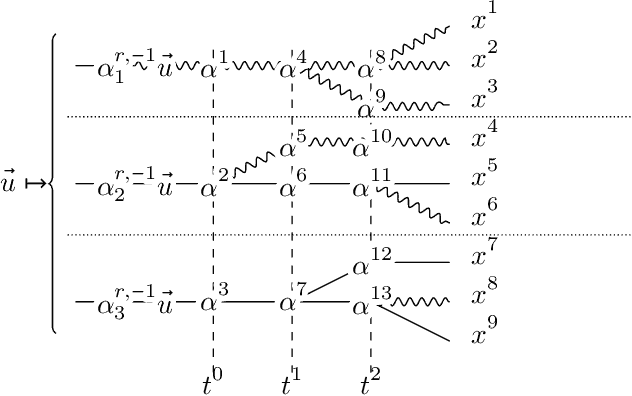
It is also denoted by $\mathrm{JAC}_{X}(f)$ or $\mathrm{JAC}(f)$. It is visualized as follows

If $s=n$, we denote by $\operatorname{Jac}{X}(f)$ or $\operatorname{Jac}{X_1, \ldots, X_n}\left(f_1, \ldots, f_n\right)$ or $\operatorname{Jac}(f)$ the Jacobian of the system $(f)$, i.e. the determinant of the Jacobian matrix.

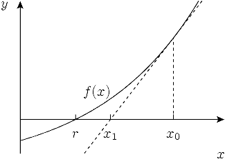
In analysis Newton’s method to approximate a root of a differentiable function $f: \mathbb{R} \rightarrow \mathbb{R}$ is the following. Starting from a point $x_0$ “near a root,” at which the derivative is “far from 0 “, we construct a series $\left(x_m\right){m \in \mathbb{N}}$ by induction by letting $$ x{m+1}=x_m-\frac{f\left(x_m\right)}{f^{\prime}\left(x_m\right)} .
$$
The method can be generalized for a system of $p$ equations with $p$ unknowns. A solution of such a system is a zero of a function $f: \mathbb{R}^p \rightarrow \mathbb{R}^p$. We apply “the same formula” as above
$$
x_{m+1}=x_m-f^{\prime}\left(x_m\right)^{-1} \cdot f\left(x_m\right),
$$
where $f^{\prime}(x)$ is the differential (the Jacobian matrix) of $f$ at the point $x \in \mathbb{R}^p$, which must be invertible in a neighborhood of $x_0$.

数学代写|交换代数代写commutative algebra代考|Definition, Changing Generator Set

A finitely presented module is an A-module $M$ given by a finite number of generators and relations. Therefore it is a module with a finite generator set having a finitely generated syzygy module. Equivalently, it is a module $M$ isomorphic to the cokernel of a linear map
$$
\gamma: \mathbf{A}^m \longrightarrow \mathbf{A}^q
$$
The matrix $G \in \mathbf{A}^{q \times m}$ of $\gamma$ has as its columns a generator set of the syzygy module between the generators $g_i$ which are the images of the canonical base of $\mathbf{A}^q$ by the surjection $\pi: \mathbf{A}^q \rightarrow M$. Such a matrix is called a presentation matrix of the module $M$ for the generator set $\left(g_1, \ldots, g_q\right)$. This translates into

$\left[g_1 \cdots g_q\right] G=0$, and
every syzygy between the $g_i$ ‘s is a linear combination of the columns of $G$, i.e.: if $\left[g_1 \cdots g_q\right] C=0$ with $C \in \mathbf{A}^{q \times 1}$, there exists a $C^{\prime} \in \mathbf{A}^{m \times 1}$ such that $C=G C^{\prime}$.

Examples
1) A free module of rank $k$ is a finitely presented module presented by a matrix column formed of $k$ zeros. ${ }^1$ More generally every simple matrix is the presentation matrix of a free module of finite rank.
2) Recall that a finitely generated projective module is a module $P$ isomorphic to the image of a projection matrix $F \in \mathbb{M}_n(\mathbf{A})$ for a specific integer $n$. Since $\mathbf{A}^n=\operatorname{Im}(F) \oplus \operatorname{Im}\left(\mathrm{I}_n-F\right)$, we obtain $P \simeq \operatorname{Coker}\left(\mathrm{I}_n-F\right)$. This shows that every finitely generated projective module is finitely presented.
3) Let $\varphi: V \rightarrow V$ be an endomorphism of a finite-dimensional vector space over a discrete field $\mathbf{K}$. Consider $V$ as a $\mathbf{K}[X]$-module with the following external law
$$
\left{\begin{aligned}
\mathbf{K}[X] \times V & \rightarrow V \
(P, u) & \mapsto P \cdot u:=P(\varphi)(u) .
\end{aligned}\right.
$$
Let $\left(u_1, \ldots, u_n\right)$ be a basis of $V$ as a $\mathbf{K}$-vector space and $A$ be the matrix of $\varphi$ with respect to this basis. Then we can show that a presentation matrix of $V$ as a $\mathbf{K}[X]$-module for the generator set $\left(u_1, \ldots, u_n\right)$ is the matrix $X \mathrm{I}_n-A$ (see Exercise 3).

交换代数代考

数学代写|交换代数代写commutative algebra代考|Newton’s Method in Algebra

让$\mathbf{k}$成为一个环，$f_1, \ldots, f_s \in \mathbf{k}[X]=\mathbf{k}\left[X_1, \ldots, X_n\right]$。系统的雅可比矩阵就是这个矩阵
$$
\mathrm{JAC}{X_1, \ldots, X_n}\left(f_1, \ldots, f_s\right)=\left(\frac{\partial f_i}{\partial X_j}\right){i \in \llbracket 1 . . s \rrbracket, j \in \llbracket 1 . . n \rrbracket} \in \mathbf{k}[X]^{s \times n} .
$$
它也用$\mathrm{JAC}_{X}(f)$或$\mathrm{JAC}(f)$表示。它可视化如下

如果$s=n$，我们用$\operatorname{Jac}{X}(f)$或$\operatorname{Jac}{X_1, \ldots, X_n}\left(f_1, \ldots, f_n\right)$或$\operatorname{Jac}(f)$表示系统$(f)$的雅可比矩阵，即雅可比矩阵的行列式。

在分析中，牛顿近似可微函数$f: \mathbb{R} \rightarrow \mathbb{R}$的根的方法如下。从一个“接近根”的点$x_0$开始，在这个点导数“远离0”，我们用归纳法构造一个级数$\left(x_m\right){m \in \mathbb{N}}$，让$$ x{m+1}=x_m-\frac{f\left(x_m\right)}{f^{\prime}\left(x_m\right)} .
$$
该方法可推广到含有$p$未知数的$p$方程组。这样一个系统的解是一个函数$f: \mathbb{R}^p \rightarrow \mathbb{R}^p$的零。我们采用与上述“相同的公式”
$$
x_{m+1}=x_m-f^{\prime}\left(x_m\right)^{-1} \cdot f\left(x_m\right),
$$
其中$f^{\prime}(x)$是$f$在$x \in \mathbb{R}^p$点的微分(雅可比矩阵)，在$x_0$的邻域内必须是可逆的。

数学代写|交换代数代写commutative algebra代考|Definition, Changing Generator Set

有限表示的模块是由有限数量的生成器和关系给出的A模块$M$。因此，它是一个具有有限生成的syzygy模块的有限发电机组模块。等价地，它是一个与线性映射的核同构的模块$M$
$$
\gamma: \mathbf{A}^m \longrightarrow \mathbf{A}^q
$$
$\gamma$的矩阵$G \in \mathbf{A}^{q \times m}$的列是生成器$g_i$之间的syzygy模块的生成集，这些生成器是通过射$\pi: \mathbf{A}^q \rightarrow M$得到的$\mathbf{A}^q$的规范基的图像。这样的矩阵称为发电机组$\left(g_1, \ldots, g_q\right)$模块$M$的表示矩阵。这转化为

$\left[g_1 \cdots g_q\right] G=0$，和

$g_i$之间的每一个协同都是$G$的列的线性组合，即:如果$\left[g_1 \cdots g_q\right] C=0$与$C \in \mathbf{A}^{q \times 1}$，则存在一个$C^{\prime} \in \mathbf{A}^{m \times 1}$，使得$C=G C^{\prime}$。

示例
1)秩为$k$的自由模块是由$k$个零组成的矩阵列表示的有限呈现模块。${ }^1$更一般地说，每个简单矩阵都是有限秩自由模的表示矩阵。
2)回想一下，一个有限生成的投影模块是一个模块$P$同构于一个特定整数$n$的投影矩阵$F \in \mathbb{M}_n(\mathbf{A})$的像。由于$\mathbf{A}^n=\operatorname{Im}(F) \oplus \operatorname{Im}\left(\mathrm{I}_n-F\right)$，我们得到$P \simeq \operatorname{Coker}\left(\mathrm{I}_n-F\right)$。这说明每一个有限生成的投影模都是有限表示的。
3)设$\varphi: V \rightarrow V$为离散场$\mathbf{K}$上有限维向量空间的自同态。将$V$视为具有以下外部律的$\mathbf{K}[X]$ -模块
$$
\left{\begin{aligned}
\mathbf{K}[X] \times V & \rightarrow V \
(P, u) & \mapsto P \cdot u:=P(\varphi)(u) .
\end{aligned}\right.
$$
设$\left(u_1, \ldots, u_n\right)$是$V$作为$\mathbf{K}$向量空间的一组基$A$是$\varphi$关于这个基的矩阵。然后我们可以证明，作为发电机组$\left(u_1, \ldots, u_n\right)$的$\mathbf{K}[X]$ -模块的表示矩阵$V$是矩阵$X \mathrm{I}_n-A$(参见练习3)。

数学代写|交换代数代写commutative algebra代考请认准statistics-lab™

统计代写请认准statistics-lab™. statistics-lab™为您的留学生涯保驾护航。

R语言代写	问卷设计与分析代写
PYTHON代写	回归分析与线性模型代写
MATLAB代写	方差分析与试验设计代写
STATA代写	机器学习/统计学习代写
SPSS代写	计量经济学代写
EVIEWS代写	时间序列分析代写
EXCEL代写	深度学习代写
SQL代写	各种数据建模与可视化代写

数学代写|交换代数代写commutative algebra代考|Algebraic Number Theory, First Steps

Posted on 2023年7月12日2023年7月12日 by statistics-lab

数学代写|交换代数代写commutative algebra代考|Algebraic Number Theory, First Steps

Here we give some general applications, in elementary number theory, of the results previously obtained in this chapter. For a glimpse of the many fascinating facets of number theory, the reader should consult the wonderful book [Ireland \& Rosen].

Integral Algebras
We give a few precisions relating to Definition 3.2.
8.1 Definition

An $\mathbf{A}$-algebra $\mathbf{B}$ is said to be finite if $\mathbf{B}$ is a finitely generated $\mathbf{A}$-module. We also say that $\mathbf{B}$ is finite over $\mathbf{A}$. In the case of an extension, we speak of a finite extension of $\mathbf{A}$.
Assume $\mathbf{A} \subseteq \mathbf{B}$. The ring $\mathbf{A}$ is said to be integrally closed in $\mathbf{B}$ if every element of $\mathbf{B}$ integral over $\mathbf{A}$ is in $\mathbf{A}$.
8.2 Fact Let $\mathbf{A} \subseteq \mathbf{B}$ and $x \in \mathbf{B}$. The following properties are equivalent.
The element $x$ is integral over $\mathbf{A}$.
The subalgebra $\mathbf{A}[x]$ of $\mathbf{B}$ is finite.
There exists a faithful and finitely generated $\mathbf{A}$-module $M \subseteq \mathbf{B}$ such that $x M \subseteq M$.

D $3 \Rightarrow 1$ (a fortiori $2 \Rightarrow 1$.) Consider a matrix $A$ with coefficients in $\mathbf{A}$ which represents $\mu_{x, M}$ (the multiplication by $x$ in $M$ ) on a finite generator set of $M$. If $f$ is the characteristic polynomial of $A$, we have by the Cayley-Hamilton theorem $0=f\left(\mu_{x, M}\right)=\mu_{f(x), M}$ and since the module is faithful, $f(x)=0$.

数学代写|交换代数代写commutative algebra代考|Concrete local-global principle

8.9 Concrete local-global principle (Integral elements) Let $S_1, \ldots$, $S_n$ be comaximal of a ring $\mathbf{A} \subseteq \mathbf{B}$ and $x \in \mathbf{B}$. We have the following equivalences.

The element $x$ is integral over $\mathbf{A}$ if and only if it is integral over each $\mathbf{A}_{S_i}$.
Assume $\mathbf{A}$ is integral, then $\mathbf{A}$ is integrally closed if and only if each $\mathbf{A}_{S_i}$ is integrally closed.

D In item 1 we need to prove that if the condition is locally achieved, then it is globally achieved. Consider then some $x \in \mathbf{B}$ which satisfies for each $i$ a relation $\left(s_i x\right)^k=a_{i, 1}\left(s_i x\right)^{k-1}+a_{i, 2}\left(s_i x\right)^{k-2}+\cdots+a_{i, k}$ with $a_{i, h} \in \mathbf{A}$ and $s_i \in S_i$ (we can assume without loss of generality that the degrees are the same). We then use a relation $\sum s_i^k u_i=1$ to obtain an integral dependence relation of $x$ over $\mathbf{A}$.
Kronecker’s theorem easily implies the following lemma.
8.10 Lemma (Kronecker’s theorem, case of an integral ring) Let A be integrally closed, and $\mathbf{K}$ be its quotient field. If we have $f=g h$ in $\mathbf{K}[T]$ with $g$, $h$ monic and $f \in \mathbf{A}[T]$, then $g$ and $h$ are also in $\mathbf{A}[T]$.
8.11 Lemma The ring $\mathbb{Z}$ as well as the ring $\mathbf{K}[X]$ when $\mathbf{K}$ is a discrete field are integrally closed.

D In fact this holds for every ring with an integral gcd A (see Sect. XI-2). Let $f(T)=T^n-\sum_{k=0}^{n-1} f_k T^k$ and $a / b$ be a reduced fraction in the quotient field of $\mathbf{A}$ with $f(a / b)=0$. By multiplying by $b^n$ we obtain
$$
a^n=b \sum_{k=0}^{n-1} f_k a^k b^{n-1-k}
$$

交换代数代考

数学代写|交换代数代写commutative algebra代考|Algebraic Number Theory, First Steps

在这里，我们给出了本章所得到的结果在初等数论中的一些一般应用。要了解数论的许多迷人方面，读者应该查阅这本精彩的书[Ireland ＆ Rosen]。

积分代数
我们给出一些与定义3.2有关的精度。
8.1定义

如果$\mathbf{B}$是有限生成的$\mathbf{A}$ -模块，则称$\mathbf{A}$ -代数$\mathbf{B}$是有限的。我们也说$\mathbf{B}$对$\mathbf{A}$是有限的。在扩展的情况下，我们说的是$\mathbf{A}$的有限扩展。

假设$\mathbf{A} \subseteq \mathbf{B}$。如果$\mathbf{B}$积分在$\mathbf{A}$上的每一个元素都在$\mathbf{A}$上，那么我们就说这个环$\mathbf{A}$在$\mathbf{B}$上是整闭的。
8.2事实让$\mathbf{A} \subseteq \mathbf{B}$和$x \in \mathbf{B}$。以下属性是等价的。

元素$x$对$\mathbf{A}$积分。

$\mathbf{B}$的子代数$\mathbf{A}[x]$是有限的。

存在一个忠实且有限生成的$\mathbf{A}$ -模块$M \subseteq \mathbf{B}$，以便$x M \subseteq M$。

D $3 \Rightarrow 1$(而不是$2 \Rightarrow 1$。)考虑一个矩阵$A$，其系数在$\mathbf{A}$中，它表示在一个有限的发电集$M$上的$\mu_{x, M}$(在$M$中乘以$x$)。如果$f$是$A$的特征多项式，我们有，根据Cayley-Hamilton定理$0=f\left(\mu_{x, M}\right)=\mu_{f(x), M}$由于模块是可靠的，$f(x)=0$。

数学代写|交换代数代写commutative algebra代考|Concrete local-global principle

8.9具体局部-全局原理(积分元)设$S_1, \ldots$, $S_n$为环的最大值$\mathbf{A} \subseteq \mathbf{B}$, $x \in \mathbf{B}$。我们有下面的等价物。

元素$x$对$\mathbf{A}$积分当且仅当它对每个$\mathbf{A}_{S_i}$积分。

假设$\mathbf{A}$是整的，那么$\mathbf{A}$是整闭的当且仅当每个$\mathbf{A}_{S_i}$是整闭的。

在第1项中，我们需要证明如果条件在局部得到满足，那么它在全局得到满足。然后考虑一些$x \in \mathbf{B}$，它满足每个$i$与$a_{i, h} \in \mathbf{A}$和$s_i \in S_i$的关系$\left(s_i x\right)^k=a_{i, 1}\left(s_i x\right)^{k-1}+a_{i, 2}\left(s_i x\right)^{k-2}+\cdots+a_{i, k}$(我们可以在不失去一般性的情况下假设度是相同的)。然后，我们使用关系$\sum s_i^k u_i=1$来获得$x$ / $\mathbf{A}$的积分依赖关系。
克罗内克定理很容易推导出以下引理。
8.10引理(Kronecker定理，积分环的情况)设A是整闭的，$\mathbf{K}$是它的商域。如果$\mathbf{K}[T]$中有$f=g h$, $g$, $h$ monic和$f \in \mathbf{A}[T]$，那么$g$和$h$也在$\mathbf{A}[T]$中。
8.11引理当$\mathbf{K}$为离散场时，环$\mathbb{Z}$和环$\mathbf{K}[X]$是整闭的。

设$f(T)=T^n-\sum_{k=0}^{n-1} f_k T^k$和$a / b$是$\mathbf{A}$与$f(a / b)=0$的商域中的约简分数。乘以$b^n$我们得到
$$
a^n=b \sum_{k=0}^{n-1} f_k a^k b^{n-1-k}
$$

统计代写请认准statistics-lab™. statistics-lab™为您的留学生涯保驾护航。

R语言代写	问卷设计与分析代写
PYTHON代写	回归分析与线性模型代写
MATLAB代写	方差分析与试验设计代写
STATA代写	机器学习/统计学习代写
SPSS代写	计量经济学代写
EVIEWS代写	时间序列分析代写
EXCEL代写	深度学习代写
SQL代写	各种数据建模与可视化代写

数学代写|交换代数代写commutative algebra代考|Dedekind-Mertens Lemma

Posted on 2023年7月12日2023年7月12日 by statistics-lab

数学代写|交换代数代写commutative algebra代考|Dedekind-Mertens Lemma

Recall that for a polynomial $f$ of $\mathbf{A}\left[X_1, \ldots, X_n\right]=\mathbf{A}[X]$, we call the “content of $f$ ” and denote by $\mathrm{c}_{\mathbf{A}, X}(f)$ or $\mathrm{c}(f)$ the ideal generated by the coefficients of $f$.

Note that we always have $\mathrm{c}(f) \mathrm{c}(g) \supseteq \mathrm{c}(f g)$ and thus $\mathrm{c}(f)^{k+1} \mathrm{c}(g) \supseteq \mathrm{c}(f)^k \mathrm{c}(f g)$ for all $k \geqslant 0$. For $k$ large enough this inclusion becomes an equality.

Dedekind-Mertens Lemma
For $f, g \in \mathbf{A}[T]$ with $m \geqslant \operatorname{deg} g$ we have $\mathrm{c}(f)^{m+1} \mathrm{c}(g)=\mathrm{c}(f)^m \mathrm{c}(f g)$.
D First of all, notice that the products $f_i g_j$ are the coefficients of the polynomial $f(Y) g(X)$. Similarly, for some indeterminates $Y_0, \ldots, Y_m$, the content of the polynomial $f\left(Y_0\right) \cdots f\left(Y_m\right) g(X)$ is equal to $\mathrm{c}(f)^{m+1} \mathrm{c}(g)$.

Let $h=f g$. Imagine that in the ring $\mathbf{B}=\mathbf{A}\left[X, Y_0, \ldots, Y_m\right]$ we are able to show the membership of the polynomial $f\left(Y_0\right) \cdots f\left(Y_m\right) g(X)$ in the ideal
$$
\sum_{j=0}^m\left(h\left(Y_j\right) \prod_{k, k \neq j}\left\langle f\left(Y_k\right)\right\rangle\right) .
$$
We would immediately deduce that $\mathrm{c}(f)^{m+1} \mathrm{c}(g) \subseteq \mathrm{c}(f)^m \mathrm{c}(h)$.
This is more or less what is going to happen. We get rid of the denominators in Lagrange’s interpolation formula (we need at least $1+\operatorname{deg} g$ interpolation points):
$$
g(X)=\sum_{j=0}^m \quad \frac{\prod_{k, k \neq j}\left(X-Y_k\right)}{\prod_{k, k \neq j}\left(Y_j-Y_k\right)} g\left(Y_j\right) .
$$
In the ring $\mathbf{B}$, by letting $\Delta=\prod_{j \neq k}\left(Y_j-Y_k\right)$, we get:
$$
\Delta \cdot g(X) \in \sum_{j=0}^m\left\langle g\left(Y_j\right)\right\rangle
$$
Thus by multiplying by $f\left(Y_0\right) \cdots f\left(Y_m\right)$ :
$$
\Delta \cdot f\left(Y_0\right) \cdots f\left(Y_m\right) \cdot g(X) \in \sum_{j=0}^m h\left(Y_j\right) \prod_{k, k \neq j}\left\langle f\left(Y_k\right)\right\rangle .
$$

数学代写|交换代数代写commutative algebra代考|A-algebras and Integral Elements

We first introduce the terminology of A-algebras. The algebras that we consider in this work are associative, commutative and unitary, unless stated otherwise.
3.1 Definition

An A-algebra is a commutative ring $\mathbf{B}$ with a homomorphism of commutative rings $\rho: \mathbf{A} \rightarrow \mathbf{B}$. That makes $\mathbf{B}$ an $\mathbf{A}$-module. When $\mathbf{A} \subseteq \mathbf{B}$, or more generally if $\rho$ is injective, we say that $\mathbf{B}$ is an extension of $\mathbf{A}$.

A morphism of the $\mathbf{A}$-algebra $\mathbf{A} \stackrel{\rho}{\longrightarrow} \mathbf{B}$ to the $\mathbf{A}$-algebra $\mathbf{A} \stackrel{\rho^{\prime}}{\longrightarrow} \mathbf{B}^{\prime}$ is a homomorphism of rings $\mathbf{B} \stackrel{\varphi}{\longrightarrow} \mathbf{B}^{\prime}$ satisfying $\varphi \circ \rho=\rho^{\prime}$. The set of morphisms of $\mathbf{A}$-algebras of $\mathbf{B}$ to $\mathbf{B}^{\prime}$ is denoted by $\operatorname{Hom}_{\mathbf{A}}\left(\mathbf{B}, \mathbf{B}^{\prime}\right)$.

Remarks
1) We chose not to reserve the terminology “extension” for the case of fields. This will require us to use in the cases of fields statements such as ” $\mathbf{L}$ is a field extension of $\mathbf{K}$ ” or ” $\mathbf{L}$ is a field, extending $\mathbf{K}$ ” from this point on.
2) Every ring is uniquely a $\mathbb{Z}$-algebra and every homomorphism of rings is a morphism of the corresponding $\mathbb{Z}$-algebras. The category of commutative rings can be regarded as a special case among the categories of algebras defined above.

Notation If $b \in \mathbf{B}$ and $M$ is a $\mathbf{B}$-module, we denote by $\mu_{M, b}$ or $\mu_b$ the multiplication by $b$ in $M: y \mapsto b y, M \rightarrow M$. This can be regarded as a $\mathbf{B}$-linear map, or, if $\mathbf{B}$ is an A-algebra, as an A-linear map for the A-module structure of $M$.
3.2 Definition Let $\mathbf{A} \subseteq \mathbf{B}$ be rings.

An element $x \in \mathbf{B}$ is said to be integral over $\mathbf{A}$ if there exists some integer $k \geqslant 1$ such that $x^k=a_1 x^{k-1}+a_2 x^{k-2}+\cdots+a_k$ with each $a_h \in \mathbf{A}$. If $\mathbf{A}$ is a discrete field, we also say that $x$ is algebraic over $\mathbf{A}$.
In this case, the monic polynomial $P=X^k-\left(a_1 X^{k-1}+a_2 X^{k-2}+\cdots+a_k\right)$ is called an integral dependence relation of $x$ over $\mathbf{A}$. In fact, by abuse of language we also say that the equality $P(x)=0$ is an integral dependence relation. If $\mathbf{A}$ is a discrete field, we also speak of an algebraic dependence relation.
The ring $\mathbf{B}$ is said to be integral over $\mathbf{A}$ if every element of $\mathbf{B}$ is integral over $\mathbf{A}$. We will also say that the $\mathbf{A}$-algebra $\mathbf{B}$ is integral. If $\mathbf{A}$ and $\mathbf{B}$ are discrete fields, we say that $\mathbf{B}$ is algebraic over $\mathbf{A}$.
If $\rho: \mathbf{C} \rightarrow \mathbf{B}$ is a $\mathbf{C}$-algebra with $\rho(\mathbf{C})=\mathbf{A}$, we say that the algebra $\mathbf{B}$ is integral over $\mathbf{C}$ if it is integral over $\mathbf{A}$.

交换代数代考

数学代写|交换代数代写commutative algebra代考|Dedekind-Mertens Lemma

回想一下，对于$\mathbf{a}\left[X_1， \ldots, X_n\right]=\mathbf{a}[X]$的多项式$f$，我们称其为“$f$的内容”，并用$\ mathm {c}_{\mathbf{a}， X}(f)$或$\ mathm {c}(f)$表示由$f$的系数产生的理想值。

注意，对于所有$k \ geqslant0 $，我们总是有$\mathrm{c}(f) \mathrm{c}(g) \supseteq \mathrm{c}(f) $和$\mathrm{c}(f)^ (k+1) \mathrm{c}(g) \supseteq \mathrm{c}(f)^k \mathrm{c}(f) $。对于足够大的$k$，这个包含变成了一个等式。

Dedekind-Mertens引理
美元的f, g \ \ mathbf{一}[T]与m美元\ geqslant \ operatorname{度}g我们有美元\ mathrm {c} (f) ^ {m + 1} \ mathrm {c} (g) = \ mathrm {c} (f) ^ m \ mathrm {c} (f (g)美元。
首先，注意乘积f_i g_j是多项式f(Y) g(X)的系数。类似地，对于一些不确定的$Y_0， \ldots, Y_m$，多项式$f\left(Y_0\right) \cdots f\left(Y_m\right) g(X)$的内容等于$\mathrm{c}(f)^{m+1} \mathrm{c}(g)$。

令$h=f g$。想象一下，在环$\mathbf{B}=\mathbf{A}\left[X, Y_0， \ldots, Y_m\right]$中，我们能够在理想情况下显示多项式$f\left(Y_0\right) \cdots f\left(Y_m\right) g(X)$的隶属性
$ $
\sum_{j=0}^m\left(h\left(Y_j\right) \prod_{k, k\ neq j}\left\langle f\left(Y_k\right)\right\rangle\right)。
$ $
我们将立即推导出$\ mathm {c}(f)^{m+1} \ mathm {c}(g) \subseteq \ mathm {c}(f)^m \ mathm {c}(h)$。
这或多或少是将要发生的事情。我们去掉拉格朗日插值公式中的分母(我们至少需要$1+\operatorname{deg} g$插值点):
$ $
g (X) = \ sum_ j = {0} ^ m \四\压裂{\ prod_ {k, k \ neq j} \离开(X-Y_k \右)}{\ prod_ {k, k \ neq j} \离开(Y_j-Y_k \右)}g \ (Y_j \右)。
$ $
在环$\mathbf{B}$中，让$\Delta=\prod_{j \neq k}\left(Y_j-Y_k\right)$，我们得到:
$ $
\Delta \cdot g(X) \in \sum_{j=0} \ m\left\langle \ g\left(Y_j\right)\right\rangle
$ $
因此，通过乘以$f\left(Y_0\right) \cdots f\left(Y_m\right)$:
$ $
\ δ \cdot f\left(Y_0\right) \cdots f\left(Y_m\right) \cdot g(X) \in \sum_{j=0}^m h\left(Y_j\right) \prod_{k, k\ neq j}\left\langle f\left(Y_k\right)\right\rangle。
$ $

数学代写|交换代数代写commutative algebra代考|A-algebras and Integral Elements

我们首先介绍a -代数的术语。除非另有说明，我们在这项工作中考虑的代数是结合的，交换的和酉的。
3.1定义

一个a代数是一个交换环$\mathbf{B}$，它具有交换环的同态$\rho: \mathbf{A} \rightarrow \mathbf{B}$。这使得$\mathbf{B}$成为$\mathbf{A}$模块。当$\mathbf{A} \subseteq \mathbf{B}$，或者更一般地说$\rho$是内射时，我们说$\mathbf{B}$是$\mathbf{A}$的扩展。

$\mathbf{A}$ -代数$\mathbf{A} \stackrel{\rho}{\longrightarrow} \mathbf{B}$到$\mathbf{A}$ -代数$\mathbf{A} \stackrel{\rho^{\prime}}{\longrightarrow} \mathbf{B}^{\prime}$的态射是满足$\varphi \circ \rho=\rho^{\prime}$的环$\mathbf{B} \stackrel{\varphi}{\longrightarrow} \mathbf{B}^{\prime}$的同态。$\mathbf{B}$到$\mathbf{B}^{\prime}$的$\mathbf{A}$ -代数的态射集合用$\operatorname{Hom}_{\mathbf{A}}\left(\mathbf{B}, \mathbf{B}^{\prime}\right)$表示。

备注
1)我们选择不为字段的情况保留术语“扩展”。这将要求我们在字段语句的情况下使用，如“$\mathbf{L}$是$\mathbf{K}$的字段扩展”或“$\mathbf{L}$是字段，扩展$\mathbf{K}$”。
2)每个环都是唯一的$\mathbb{Z}$ -代数，每个环的同态是对应的$\mathbb{Z}$ -代数的态射。交换环的范畴可以看作是上述代数范畴中的一个特例。

如果$b \in \mathbf{B}$和$M$是$\mathbf{B}$ -模块，我们用$\mu_{M, b}$或$\mu_b$表示$M: y \mapsto b y, M \rightarrow M$中与$b$的乘法。这可以视为$\mathbf{B}$ -线性映射，或者，如果$\mathbf{B}$是a -代数，则可以视为$M$的a -模块结构的a -线性映射。
3.2定义设$\mathbf{A} \subseteq \mathbf{B}$为环。

如果存在一个整数$k \geqslant 1$，使得每个$a_h \in \mathbf{A}$对应一个整数$x^k=a_1 x^{k-1}+a_2 x^{k-2}+\cdots+a_k$，则称元素$x \in \mathbf{B}$是对$\mathbf{A}$的整数。如果$\mathbf{A}$是一个离散域，我们也说$x$是对$\mathbf{A}$的代数。

在这种情况下，一元多项式$P=X^k-\left(a_1 X^{k-1}+a_2 X^{k-2}+\cdots+a_k\right)$被称为$x$ / $\mathbf{A}$的积分依赖关系。其实，滥用语言，我们也可以说等式$P(x)=0$是一种整体依赖关系。如果$\mathbf{A}$是一个离散域，我们也说代数依赖关系。

如果$\mathbf{B}$的每一个元素都是$\mathbf{A}$的积分，那么这个环$\mathbf{B}$就是对$\mathbf{A}$的积分。我们也可以说$\mathbf{A}$ -代数$\mathbf{B}$是积分。如果$\mathbf{A}$和$\mathbf{B}$是离散域，我们说$\mathbf{B}$是对$\mathbf{A}$的代数。

如果$\rho: \mathbf{C} \rightarrow \mathbf{B}$和$\rho(\mathbf{C})=\mathbf{A}$是一个$\mathbf{C}$ -代数，我们说$\mathbf{B}$是对$\mathbf{C}$的积分如果它是对$\mathbf{A}$的积分。

统计代写请认准statistics-lab™. statistics-lab™为您的留学生涯保驾护航。

R语言代写	问卷设计与分析代写
PYTHON代写	回归分析与线性模型代写
MATLAB代写	方差分析与试验设计代写
STATA代写	机器学习/统计学习代写
SPSS代写	计量经济学代写
EVIEWS代写	时间序列分析代写
EXCEL代写	深度学习代写
SQL代写	各种数据建模与可视化代写

数学代写|交换代数代写commutative algebra代考|Injectivity and Surjectivity Criteria

Posted on 2023年6月28日2023年6月28日 by statistics-lab

数学代写|交换代数代写commutative algebra代考|Injectivity and Surjectivity Criteria

Two famous propositions are contained in the following theorem.
Theorem Let $\varphi: \mathbf{A}^n \rightarrow \mathbf{A}^m$ be a linear map with matrix $A$.

The map $\varphi$ is surjective if and only if $\varphi$ is of rank $m$, i.e. here $\mathcal{D}_m(\varphi)=\langle 1\rangle$ (we then say that $A$ is unimodular).

(McCoy’s theorem) The map $\varphi$ is injective if and only if $\mathcal{D}_n(\varphi)$ is faithful, i.e. if the annihilator of $\mathcal{D}_n(\varphi)$ is reduced to ${0}$.

D 1. If $\varphi$ is surjective, it admits a right inverse $\psi$, and Fact 5.6 gives $\langle 1\rangle=\mathcal{D}_m\left(\mathrm{I}_m\right) \subseteq$ $\mathcal{D}_m(\varphi) \mathcal{D}_m(\psi)$, so $\mathcal{D}_m(\varphi)=\langle 1\rangle$. Conversely, if $A$ is of rank $m$, Eq. (18) shows that $A$ admits a right inverse, and $\varphi$ is surjective.

Assume that $\mathcal{D}n(A)$ is faithful. By equality (16), if $A V=0$, then $\mu{\alpha, 1 . . n} V=0$ for all the generators $\mu_{\alpha, 1 . . n}$ of $\mathcal{D}n(A)$, and so $V=0$. For the converse, we will prove by induction on $k$ the following property: if $k$ column vectors $x_1, \ldots, x_k$ are linearly independent, then the annihilator of the vector $x_1 \wedge \cdots \wedge x_k$ is reduced to 0 . For $k=1$ it is trivial. To pass from $k$ to $k+1$ we proceed as follows. Let $z$ be a scalar that annihilates $x_1 \wedge \cdots \wedge x{k+1}$. For $\alpha \in \mathcal{P}{k, m}$, we denote by $d\alpha\left(y_1, \ldots, y_k\right)$ the minor extracted on the index rows of $\alpha$ for the column vectors $y_1, \ldots, y_k$ of $\mathbf{A}^m$. Since $z\left(x_1 \wedge \cdots \wedge x_{k+1}\right)=0$, and by the Cramer formulas, we have the equality
$$
z\left(d_\alpha\left(x_1, \ldots, x_k\right) x_{k+1}-d_\alpha\left(x_1, \ldots, x_{k-1}, x_{k+1}\right) x_k+\cdots\right)=0
$$
so $z d_\alpha\left(x_1, \ldots, x_k\right)=0$
As this is true for any $\alpha$, this gives $z\left(x_1 \wedge \cdots \wedge x_k\right)=0$, and by the induction hypothesis, $z=0$.

数学代写|交换代数代写commutative algebra代考|Characterization of Locally Simple Maps

The following lemma places a bijective correspondence between the fundamental systems of orthogonal idempotents and the non-decreasing sequences of idempotents for divisibility.
5.25 Lemma Let $\left(e_{q+1}=0, e_q, \ldots, e_1, e_0=1\right)$ be a list of idempotents such that $e_i$ divides $e_{i+1}$ for $i=0, \ldots$, . Then, the elements $r_i:=e_i-e_{i+1}$, for $i \in \llbracket 0 . . q \rrbracket$, form a fundamental system of orthogonal idempotents. Conversely, every fundamental system of orthogonal idempotents $\left(r_0, \ldots, r_q\right)$ defines such a list of idempotents by letting
$$
e_j=\sum_{k \geqslant j} r_k \text { for } j \in \llbracket 0 . . q+1 \rrbracket
$$
D It is clear that $\sum_i r_i=1$. For $0 \leqslant ii$.

We denote by $\operatorname{Diag}\left(a_1, \ldots, a_n\right)$ the diagonal matrix of order $n$ whose coefficient in position $(i, i)$ is the element $a_i$.

In the following theorem some of the idempotents $r_i$ in the fundamental system of orthogonal idempotents can very well be equal to zero. For example if the ring is connected and nontrivial, all but one are equal to zero.

5.26 Theorem (Locally simple matrix) Let $G \in \mathbf{A}^{m \times n}$ be the matrix of $\varphi: \mathbf{A}^n \rightarrow \mathbf{A}^m$ and $q=\inf (m, n)$.
The following properties are equivalent.

The linear map $\varphi$ is locally simple.
The submodule $\operatorname{Im} \varphi$ is a direct summand of $\mathbf{A}^m$.
$\operatorname{Im} \varphi$ is a direct summand of $\mathbf{A}^m$ and $\operatorname{Ker} \varphi$ is a direct summand of $\mathbf{A}^n$.
There exists a linear map $\varphi^{\bullet}: \mathbf{A}^m \rightarrow \mathbf{A}^n$ with $\mathbf{A}^n=\operatorname{Ker} \varphi \oplus \operatorname{Im} \varphi^{\bullet}$ and $\mathbf{A}^m=\operatorname{Ker} \varphi^{\bullet} \oplus \operatorname{Im} \varphi$.
Each determinantal ideal $\mathcal{D}_k(\varphi)$ is idempotent.
There exists a (unique) fundamental system of orthogonal idempotents $\left(r_0, r_1\right.$, $\ldots, r_q$ ) such that on each localized ring $\mathbf{A}\left[1 / r_k\right]$ the map $\varphi$ is of rank $k$.
Each determinantal ideal $\mathcal{D}k(\varphi)$ is generated by an idempotent $e_k$. Then let $r_k=e_k-e{k+1}$. The $r_k$ ‘s form a fundamental system of orthogonal idempotents. For every minor $\mu$ of order $k$ of $G$, on the localized ring $\mathbf{A}\left[1 /\left(r_k \mu\right)\right]$ the linear map $\varphi$ becomes simple of rank $k$.
The linear map $\varphi$ becomes simple after localization at suitable comaximal elements.
Each determinantal ideal $\mathcal{D}_k(\varphi)$ is generated by an idempotent $e_k$ and the matrix of $\varphi$ becomes equivalent to the matrix $\operatorname{Diag}\left(e_1, e_2, \ldots, e_q\right)$, eventually filled-in with zeros (for both rows and columns), after localization at suitable comaximal elements.
${ }^{\star}$ The linear map $\varphi$ becomes simple after localization at any arbitrary maximal ideal.

交换代数代考

数学代写|交换代数代写commutative algebra代考|Injectivity and Surjectivity Criteria

下面的定理包含了两个著名的命题。
设$\varphi: \mathbf{A}^n \rightarrow \mathbf{A}^m$为矩阵$A$的线性映射。

映射$\varphi$是满射的当且仅当$\varphi$的秩为$m$，即这里为$\mathcal{D}_m(\varphi)=\langle 1\rangle$(然后我们说$A$是单模的)。

(McCoy定理)当且仅当$\mathcal{D}_n(\varphi)$是忠实的，即$\mathcal{D}_n(\varphi)$的湮灭子约化为${0}$，映射$\varphi$是内射的。

解析:选D。如果$\varphi$是满射，它就有一个右逆$\psi$，而事实5.6给出$\langle 1\rangle=\mathcal{D}_m\left(\mathrm{I}_m\right) \subseteq$$\mathcal{D}_m(\varphi) \mathcal{D}_m(\psi)$，所以$\mathcal{D}_m(\varphi)=\langle 1\rangle$。反之，如果$A$的秩为$m$，则Eq.(18)表明$A$存在右逆，$\varphi$是满射。

假设$\mathcal{D}n(A)$是忠实的。通过等式(16)，如果$A V=0$，那么对于$\mathcal{D}n(A)$的所有生成器$\mu_{\alpha, 1 . . n}$为$\mu{\alpha, 1 . . n} V=0$，因此$V=0$。反之，我们将通过归纳法在$k$上证明以下性质:如果$k$列向量$x_1, \ldots, x_k$是线性无关的，则向量$x_1 \wedge \cdots \wedge x_k$的湮灭子约为0。对于$k=1$来说，这是微不足道的。要从$k$传递到$k+1$，我们进行如下操作。假设$z$是一个能湮灭$x_1 \wedge \cdots \wedge x{k+1}$的标量。对于$\alpha \in \mathcal{P}{k, m}$，我们用$d\alpha\left(y_1, \ldots, y_k\right)$表示在$\alpha$的索引行上为$\mathbf{A}^m$的列向量$y_1, \ldots, y_k$提取的次要值。因为$z\left(x_1 \wedge \cdots \wedge x_{k+1}\right)=0$，通过克莱默公式，我们得到了等式
$$
z\left(d_\alpha\left(x_1, \ldots, x_k\right) x_{k+1}-d_\alpha\left(x_1, \ldots, x_{k-1}, x_{k+1}\right) x_k+\cdots\right)=0
$$
所以$z d_\alpha\left(x_1, \ldots, x_k\right)=0$
因为这对任何$\alpha$都成立，所以得到$z\left(x_1 \wedge \cdots \wedge x_k\right)=0$，根据归纳假设，得到$z=0$。

数学代写|交换代数代写commutative algebra代考|Characterization of Locally Simple Maps

下面的引理在正交幂等元的基本系统和幂等元的可整除的非递减序列之间建立了双射对应关系。
5.25引理设$\left(e_{q+1}=0, e_q, \ldots, e_1, e_0=1\right)$是一个幂等函数列表，使得$e_i$除$e_{i+1}$等于$i=0, \ldots$，。然后，对于$i \in \llbracket 0 . . q \rrbracket$，元素$r_i:=e_i-e_{i+1}$形成一个正交幂等元的基本系统。相反，每一个正交幂等元的基本系统$\left(r_0, \ldots, r_q\right)$定义了这样一个幂等元列表，让
$$
e_j=\sum_{k \geqslant j} r_k \text { for } j \in \llbracket 0 . . q+1 \rrbracket
$$
很明显，$\sum_i r_i=1$。浏览$0 \leqslant ii$。

我们用$\operatorname{Diag}\left(a_1, \ldots, a_n\right)$表示阶为$n$的对角矩阵，其位置$(i, i)$的系数为元素$a_i$。

在下面的定理中，正交幂等元的基本体系中的一些幂等元$r_i$可以很好地等于零。例如，如果环是连通且非平凡的，则除一个环外其他环都等于零。

5.26定理(局部简单矩阵)设$G \in \mathbf{A}^{m \times n}$为$\varphi: \mathbf{A}^n \rightarrow \mathbf{A}^m$和$q=\inf (m, n)$的矩阵。
以下属性是等价的。

线性地图$\varphi$是局部简单的。

子模块$\operatorname{Im} \varphi$是$\mathbf{A}^m$的直接和。

$\operatorname{Im} \varphi$ 是$\mathbf{A}^m$的直接和，$\operatorname{Ker} \varphi$是$\mathbf{A}^n$的直接和。

存在一个线性映射$\varphi^{\bullet}: \mathbf{A}^m \rightarrow \mathbf{A}^n$与$\mathbf{A}^n=\operatorname{Ker} \varphi \oplus \operatorname{Im} \varphi^{\bullet}$和$\mathbf{A}^m=\operatorname{Ker} \varphi^{\bullet} \oplus \operatorname{Im} \varphi$。

每个行列式理想$\mathcal{D}_k(\varphi)$都是幂等的。

存在一个(唯一的)正交幂等元的基本系统$\left(r_0, r_1\right.$, $\ldots, r_q$)，使得在每个定域环$\mathbf{A}\left[1 / r_k\right]$上映射$\varphi$的秩为$k$。

每个行列式理想$\mathcal{D}k(\varphi)$都是由一个幂等的$e_k$生成的。然后让$r_k=e_k-e{k+1}$。$r_k$形成了一个正交幂等函数的基本体系。对于$G$阶为$k$的每一个次次$\mu$，在定域环$\mathbf{A}\left[1 /\left(r_k \mu\right)\right]$上，线性映射$\varphi$的阶为$k$。

线性图$\varphi$在合适的最大元素处定位后变得简单。

每个行列式理想$\mathcal{D}_k(\varphi)$都是由一个幂等的$e_k$生成的，而$\varphi$的矩阵就等于矩阵$\operatorname{Diag}\left(e_1, e_2, \ldots, e_q\right)$，在适当的极大值元素处定位后，最终用零填充(对于行和列)。

${ }^{\star}$ 线性图$\varphi$在任意最大理想定位后变得简单。

统计代写请认准statistics-lab™. statistics-lab™为您的留学生涯保驾护航。

金融工程代写

金融工程是使用数学技术来解决金融问题。金融工程使用计算机科学、统计学、经济学和应用数学领域的工具和知识来解决当前的金融问题，以及设计新的和创新的金融产品。

非参数统计代写

非参数统计指的是一种统计方法，其中不假设数据来自于由少数参数决定的规定模型；这种模型的例子包括正态分布模型和线性回归模型。

广义线性模型代考

广义线性模型（GLM）归属统计学领域，是一种应用灵活的线性回归模型。该模型允许因变量的偏差分布有除了正态分布之外的其它分布。

术语广义线性模型（GLM）通常是指给定连续和/或分类预测因素的连续响应变量的常规线性回归模型。它包括多元线性回归，以及方差分析和方差分析（仅含固定效应）。

有限元方法代写

有限元方法（FEM）是一种流行的方法，用于数值解决工程和数学建模中出现的微分方程。典型的问题领域包括结构分析、传热、流体流动、质量运输和电磁势等传统领域。

有限元是一种通用的数值方法，用于解决两个或三个空间变量的偏微分方程（即一些边界值问题）。为了解决一个问题，有限元将一个大系统细分为更小、更简单的部分，称为有限元。这是通过在空间维度上的特定空间离散化来实现的，它是通过构建对象的网格来实现的：用于求解的数值域，它有有限数量的点。边界值问题的有限元方法表述最终导致一个代数方程组。该方法在域上对未知函数进行逼近。[1] 然后将模拟这些有限元的简单方程组合成一个更大的方程系统，以模拟整个问题。然后，有限元通过变化微积分使相关的误差函数最小化来逼近一个解决方案。

tatistics-lab作为专业的留学生服务机构，多年来已为美国、英国、加拿大、澳洲等留学热门地的学生提供专业的学术服务，包括但不限于Essay代写，Assignment代写，Dissertation代写，Report代写，小组作业代写，Proposal代写，Paper代写，Presentation代写，计算机作业代写，论文修改和润色，网课代做，exam代考等等。写作范围涵盖高中，本科，研究生等海外留学全阶段，辐射金融，经济学，会计学，审计学，管理学等全球99%专业科目。写作团队既有专业英语母语作者，也有海外名校硕博留学生，每位写作老师都拥有过硬的语言能力，专业的学科背景和学术写作经验。我们承诺100%原创，100%专业，100%准时，100%满意。

随机分析代写

随机微积分是数学的一个分支，对随机过程进行操作。它允许为随机过程的积分定义一个关于随机过程的一致的积分理论。这个领域是由日本数学家伊藤清在第二次世界大战期间创建并开始的。

时间序列分析代写

随机过程，是依赖于参数的一组随机变量的全体，参数通常是时间。随机变量是随机现象的数量表现，其时间序列是一组按照时间发生先后顺序进行排列的数据点序列。通常一组时间序列的时间间隔为一恒定值（如1秒，5分钟，12小时，7天，1年），因此时间序列可以作为离散时间数据进行分析处理。研究时间序列数据的意义在于现实中，往往需要研究某个事物其随时间发展变化的规律。这就需要通过研究该事物过去发展的历史记录，以得到其自身发展的规律。

回归分析代写

多元回归分析渐进（Multiple Regression Analysis Asymptotics）属于计量经济学领域，主要是一种数学上的统计分析方法，可以分析复杂情况下各影响因素的数学关系，在自然科学、社会和经济学等多个领域内应用广泛。

MATLAB代写

MATLAB 是一种用于技术计算的高性能语言。它将计算、可视化和编程集成在一个易于使用的环境中，其中问题和解决方案以熟悉的数学符号表示。典型用途包括：数学和计算算法开发建模、仿真和原型制作数据分析、探索和可视化科学和工程图形应用程序开发，包括图形用户界面构建MATLAB 是一个交互式系统，其基本数据元素是一个不需要维度的数组。这使您可以解决许多技术计算问题，尤其是那些具有矩阵和向量公式的问题，而只需用 C 或 Fortran 等标量非交互式语言编写程序所需的时间的一小部分。MATLAB 名称代表矩阵实验室。MATLAB 最初的编写目的是提供对由 LINPACK 和 EISPACK 项目开发的矩阵软件的轻松访问，这两个项目共同代表了矩阵计算软件的最新技术。MATLAB 经过多年的发展，得到了许多用户的投入。在大学环境中，它是数学、工程和科学入门和高级课程的标准教学工具。在工业领域，MATLAB 是高效研究、开发和分析的首选工具。MATLAB 具有一系列称为工具箱的特定于应用程序的解决方案。对于大多数 MATLAB 用户来说非常重要，工具箱允许您学习和应用专业技术。工具箱是 MATLAB 函数（M 文件）的综合集合，可扩展 MATLAB 环境以解决特定类别的问题。可用工具箱的领域包括信号处理、控制系统、神经网络、模糊逻辑、小波、仿真等。

R语言代写	问卷设计与分析代写
PYTHON代写	回归分析与线性模型代写
MATLAB代写	方差分析与试验设计代写
STATA代写	机器学习/统计学习代写
SPSS代写	计量经济学代写
EVIEWS代写	时间序列分析代写
EXCEL代写	深度学习代写
SQL代写	各种数据建模与可视化代写

数学代写|交换代数代写commutative algebra代考|Free Submodules as Direct Summands (Splitting Off)

Posted on 2023年6月28日2023年6月28日 by statistics-lab

数学代写|交换代数代写commutative algebra代考|Free Submodules as Direct Summands (Splitting Off)

Let $k \in \mathbb{N}$. A free module of rank $k$ is by definition an $\mathbf{A}$-module isomorphic to $\mathbf{A}^k$. If $k$ is not specified, we will say free module of finite rank.

When $\mathbf{A}$ is a discrete field we speak of a finite dimensional vector space or a finite rank vector space interchangeably.

The modules whose structure is the simplest are the free modules of finite rank. We are thus interested in the possibility of constructing an arbitrary module $M$ in the form $L \oplus N$ where $L$ is a free module of finite rank. A (partial) answer to this question is given by the exterior algebra.
5.1 Proposition (Splitting Off) Let $a_1, \ldots, a_k$ be elements of an $\mathbf{A}$-module $M$, then the following properties are equivalent.

The submodule $L=\left\langle a_1, \ldots, a_k\right\rangle$ of $M$ is free with basis $\left(a_1, \ldots, a_k\right)$ and is $a$ direct summand of $M$.

There exists a k-multilinear alternating form $\varphi: M^k \rightarrow \mathbf{A}$ which satisfies the equality $\varphi\left(a_1, \ldots, a_k\right)=1$.

D $1 \Rightarrow 2$. If $L \oplus N=M$, if $\pi: M \rightarrow L$ is the projection parallel to $N$, and if $\theta_j: L \rightarrow \mathbf{A}$ is the $j$-th coordinate form for the basis $\left(a_1, \ldots, a_k\right)$, we define
$$
\varphi\left(x_1, \ldots, x_k\right)=\operatorname{det}\left(\left(\theta_j\left(\pi\left(x_i\right)\right)\right){i, j \in \llbracket 1 . . k \rrbracket}\right) . $$ $2 \Rightarrow 1$. We define the linear map $\pi: M \rightarrow M$ as $$ \pi(x)=\sum{j=1}^k \varphi(\underbrace{a_1, \ldots, x, \ldots, a_k}_{(x \text { is in position } j)}) a_j .
$$

We immediately have $\pi\left(a_i\right)=a_i$ and $\operatorname{Im} \pi \subseteq L:=\left\langle a_1, \ldots, a_k\right\rangle$, thus $\pi^2=\pi$ and $\operatorname{Im} \pi=L$. Finally, if $x=\sum_j \lambda_j a_j=0$, then $\varphi\left(a_1, \ldots, x, \ldots, a_k\right)=\lambda_j=0$ (with $x$ in position $j$ ).

Special case: for $k=1$ we say that the element $a_1$ of $M$ is unimodular when there exists a linear form $\varphi: M \rightarrow \mathbf{A}$ such that $\varphi\left(a_1\right)=1$. The vector $b=\left(b_1, \ldots, b_n\right) \in$ $\mathbf{A}^n$ is unimodular if and only if the $b_i$ ‘s are comaximal. In this case we also say that the sequence $\left(b_1, \ldots, b_n\right)$ is unimodular.

数学代写|交换代数代写commutative algebra代考|The Rank of a Free Module

As we will see, the rank of a free module is a well-determined integer if the ring is nontrivial. In other words, two $\mathbf{A}$-modules $M \simeq \mathbf{A}^m$ and $P \simeq \mathbf{A}^p$ with $m \neq p$ can only be isomorphic if $1={ }_{\mathbf{A}} 0$.

We will use the notation $\operatorname{rk}_{\mathbf{A}}(M)=k$ (or rk $(M)=k$ if $\mathbf{A}$ is clear from the context) to indicate that a (supposedly free) module has rank $k$.

A scholarly proof consists to say that, if $m>p$, the $m$-th exterior power of $P$ is ${0}$ whereas that of $M$ is isomorphic to $\mathbf{A}$ (this is essentially the proof for Corollary 5.23).
The same proof can be presented in a more elementary way as follows. First recall the basic Cramer formula. If $B$ is a square matrix of order $n$, we denote by $\widetilde{B}$ or $\operatorname{Adj} B$ the cotransposed matrix (sometimes called adjoint). The elementary form of Cramer’s identities is then expressed as:
$$
A \operatorname{Adj}(A)=\operatorname{Adj}(A) A=\operatorname{det}(A) \mathrm{I}_n .
$$
This formula, in combination with the product formula
$$
\operatorname{det}(A B)=\operatorname{det}(A) \operatorname{det}(B)
$$
has a couple of implications regarding square matrices. First, that a square matrix $A$ is invertible on one side if and only if $A$ is invertible if and only if its determinant is invertible. Second, that the inverse of $A$ is equal to $(\operatorname{det} A)^{-1} \operatorname{Adj} A$.

We now consider two $\mathbf{A}$-modules $M \simeq \mathbf{A}^m$ and $P \simeq \mathbf{A}^p$ with $m \geqslant p$ and a surjective linear map $\varphi: P \rightarrow M$. Therefore there exists a linear map $\psi: M \rightarrow P$ such that $\varphi \circ \psi=\operatorname{Id}_M$. This corresponds to two matrices $A \in \mathbf{A}^{m \times p}$ and $B \in \mathbf{A}^{p \times m}$ with $A B=\mathrm{I}_m$. If $m=p$, the matrix $A$ is invertible with inverse $B$ and $\varphi$ and $\psi$ are reciprocal isomorphisms. If $m>p$, we have $A B=A_1 B_1$ with square $A_1$ and $B_1$ respectively obtained from $A$ and $B$ by filling in with zeros ( $m-p$ columns for $A_1$, $m-p$ rows for $B_1$ ).

交换代数代考

数学代写|交换代数代写commutative algebra代考|Free Submodules as Direct Summands (Splitting Off)

让$k \in \mathbb{N}$。根据定义，秩为$k$的自由模块是与$\mathbf{A}^k$同构的$\mathbf{A}$ -模块。如果没有指定$k$，我们将说有限秩的自由模块。

当$\mathbf{A}$是一个离散域时，我们可以交替地说有限维向量空间或有限秩向量空间。

结构最简单的模是有限秩的自由模。因此，我们对以$L \oplus N$的形式构造任意模块$M$的可能性感兴趣，其中$L$是有限秩的自由模块。外部代数给出了这个问题的(部分)答案。
5.1命题(分离)设$a_1, \ldots, a_k$为$\mathbf{A}$ -模块$M$的元素，则下列属性是等价的。

$M$的子模块$L=\left\langle a_1, \ldots, a_k\right\rangle$与基础$\left(a_1, \ldots, a_k\right)$是免费的，并且是$M$的直接求和$a$。

存在k-多线性交替形式$\varphi: M^k \rightarrow \mathbf{A}$满足等式$\varphi\left(a_1, \ldots, a_k\right)=1$。

D $1 \Rightarrow 2$。如果$L \oplus N=M$，如果$\pi: M \rightarrow L$是平行于$N$的投影，如果$\theta_j: L \rightarrow \mathbf{A}$是基$\left(a_1, \ldots, a_k\right)$的$j$ -坐标形式，我们定义
$$
\varphi\left(x_1, \ldots, x_k\right)=\operatorname{det}\left(\left(\theta_j\left(\pi\left(x_i\right)\right)\right){i, j \in \llbracket 1 . . k \rrbracket}\right) . $$$2 \Rightarrow 1$。我们将线性映射$\pi: M \rightarrow M$定义为 $$ \pi(x)=\sum{j=1}^k \varphi(\underbrace{a_1, \ldots, x, \ldots, a_k}_{(x \text { is in position } j)}) a_j .
$$

我们马上得到$\pi\left(a_i\right)=a_i$和$\operatorname{Im} \pi \subseteq L:=\left\langle a_1, \ldots, a_k\right\rangle$，也就是$\pi^2=\pi$和$\operatorname{Im} \pi=L$。最后，如果是$x=\sum_j \lambda_j a_j=0$，那么是$\varphi\left(a_1, \ldots, x, \ldots, a_k\right)=\lambda_j=0$ ($x$的位置是$j$)。

特殊情况:对于$k=1$，我们说$M$的元素$a_1$是单模的，当存在一个线性形式$\varphi: M \rightarrow \mathbf{A}$，使得$\varphi\left(a_1\right)=1$。向量$b=\left(b_1, \ldots, b_n\right) \in$$\mathbf{A}^n$是单模的当且仅当$b_i$是最大的。在这种情况下，我们也说序列$\left(b_1, \ldots, b_n\right)$是单模的。

数学代写|交换代数代写commutative algebra代考|The Rank of a Free Module

正如我们将看到的，如果环是非平凡的，则自由模的秩是一个确定的整数。换句话说，两个$\mathbf{A}$ -模块$M \simeq \mathbf{A}^m$和$P \simeq \mathbf{A}^p$与$m \neq p$只能是同构的，如果$1={ }_{\mathbf{A}} 0$。

我们将使用表示法$\operatorname{rk}_{\mathbf{A}}(M)=k$(如果上下文中明确表示$\mathbf{A}$，则使用rk $(M)=k$)来表示(假定为自由的)模块的等级为$k$。

一个学术证明包括说，如果$m>p$, $P$的$m$ -th外部幂是${0}$，而$M$的 -th外部幂是$\mathbf{A}$同构的(这实质上是推论5.23的证明)。
同样的证明可以用一种更基本的方式表示如下。首先回想一下克拉默的基本公式。如果$B$是一个阶为$n$的方阵，我们用$\widetilde{B}$或$\operatorname{Adj} B$表示协置矩阵(有时称为伴随矩阵)。Cramer恒等式的初等形式表示为:
$$
A \operatorname{Adj}(A)=\operatorname{Adj}(A) A=\operatorname{det}(A) \mathrm{I}_n .
$$
这个公式，结合乘积公式
$$
\operatorname{det}(A B)=\operatorname{det}(A) \operatorname{det}(B)
$$
有一些关于方阵的含义。首先，一个方阵$A$在一边可逆当且仅当$A$可逆当且仅当它的行列式可逆。第二，$A$的倒数等于$(\operatorname{det} A)^{-1} \operatorname{Adj} A$。

现在我们考虑两个$\mathbf{A}$ -模块$M \simeq \mathbf{A}^m$和$P \simeq \mathbf{A}^p$，其中包含$m \geqslant p$和一个满射线性映射$\varphi: P \rightarrow M$。因此存在一个线性映射$\psi: M \rightarrow P$，使得$\varphi \circ \psi=\operatorname{Id}_M$。这对应于两个矩阵$A \in \mathbf{A}^{m \times p}$和$B \in \mathbf{A}^{p \times m}$和$A B=\mathrm{I}_m$。如果$m=p$，则矩阵$A$可逆且逆$B$，且$\varphi$和$\psi$是互易同构的。如果$m>p$，我们有$A B=A_1 B_1$与$A_1$和$B_1$分别从$A$和$B$通过填零得到($m-p$列为$A_1$, $m-p$行为$B_1$)。

统计代写请认准statistics-lab™. statistics-lab™为您的留学生涯保驾护航。

金融工程代写

非参数统计代写

非参数统计指的是一种统计方法，其中不假设数据来自于由少数参数决定的规定模型；这种模型的例子包括正态分布模型和线性回归模型。

广义线性模型代考

广义线性模型（GLM）归属统计学领域，是一种应用灵活的线性回归模型。该模型允许因变量的偏差分布有除了正态分布之外的其它分布。

有限元方法代写

随机分析代写

时间序列分析代写

回归分析代写

MATLAB代写

R语言代写	问卷设计与分析代写
PYTHON代写	回归分析与线性模型代写
MATLAB代写	方差分析与试验设计代写
STATA代写	机器学习/统计学习代写
SPSS代写	计量经济学代写
EVIEWS代写	时间序列分析代写
EXCEL代写	深度学习代写
SQL代写	各种数据建模与可视化代写

数学代写|交换代数代写commutative algebra代考|Some Facts Concerning Quotients and Localizations

Posted on 2023年6月28日2023年6月28日 by statistics-lab

数学代写|交换代数代写commutative algebra代考|Some Facts Concerning Quotients and Localizations

Let us begin by recalling the following result on quotients. Let $\mathfrak{a}$ be an ideal of a ring $\mathbf{A}$. When needed, the canonical mapping will be denoted by $\pi_{\mathbf{A}, \mathfrak{a}}: \mathbf{A} \rightarrow \mathbf{A} / \mathfrak{a}$.
The quotient ring $\left(\mathbf{A} / \mathfrak{a}, \pi_{\mathbf{A}, \mathfrak{a}}\right)$ is characterized, up to unique isomorphism, by the following universal property.
Fact (Characteristic property of the quotient by the ideal a) A ring homomorphism $\psi: \mathbf{A} \rightarrow \mathbf{B}$ is factorized by $\pi_{\mathbf{A}, \mathfrak{a}}$ if and only if $\mathfrak{a} \subseteq \operatorname{Ker} \psi$, meaning $\psi(\mathfrak{a}) \subseteq\left{0_{\mathbf{B}}\right}$. In this case, the factorization is unique.

Explanation regarding the figure. In a figure of the type found above, everything but the morphism $\theta$ corresponding to the dotted arrow is given. The exclamation mark signifies that $\theta$ makes the diagram commute and that it is the unique morphism with this property.

We denote by $M / \mathfrak{a} M$ the $\mathbf{A} / \mathfrak{a}$-module obtained from the quotient of the $\mathbf{A}$-module $M$ by the submodule generated by the elements $a x$ for $a \in \mathfrak{a}$ and $x \in M$. This module can thus be defined through the extension of scalars to $\mathbf{A} / \mathfrak{a}$ from the $\mathbf{A}$-module $M$ (see p. 191, and Exercise IV-5).

Let us move on to localizations, which are very analogous to quotients (we will return to this analogy in further detail on p. 635). In this work, when referring to a monoid contained within a ring (i.e. a submonoid of a ring) we always assume a subset of the ring which contains 1 and is closed under multiplication.

For a given ring $\mathbf{A}$, we denote by $\mathbf{A}^{\times}$the multiplicative group of invertible elements, also called the group of units.

If $S$ is a monoid, we denote by $\mathbf{A}_S$ or $S^{-1} \mathbf{A}$ the localization of $\mathbf{A}$ at $S$. Every element of $\mathbf{A}_S$ can be written in the form $x / s$ with $x \in \mathbf{A}$ and $s \in S$.

By definition we have $x_1 / s_1=x_2 / s_2$ if there exists an $s \in S$ such that $s s_2 x_1=$ $s s_1 x_2$. When needed, we will denote by $j_{\mathbf{A}, S}: \mathbf{A} \rightarrow \mathbf{A}_S$ the canonical mapping $x \mapsto x / 1$

The localized ring $\left(\mathbf{A}S, j{\mathbf{A}, S}\right)$ is characterized, up to unique isomorphism, by the following universal property.

数学代写|交换代数代写commutative algebra代考|The Basic Local-Global Principle

We will study the general workings of the local-global principle in commutative algebra in Chap. XV. However, we will encounter it at every turn, under different forms adapted to each situation. In this section, an essential instance of this principle is given as it is so simple and efficient that it would be a pity to go without it any longer.

The local-global principle affirms that certain properties are true if and only if they are true after “sufficiently many” localizations. In classical mathematics we often invoke localization at every maximal ideal. It is a lot of work and seems a bit mysterious, especially from an algorithmic point of view. We will use simpler (and less intimidating) versions in which only a finite number of localizations are used.
Comaximal Localizations and the Local-Global Principle
The following definition corresponds to the intuitive idea that certain (finite) systems of localizations of a ring $\mathbf{A}$ are “sufficiently numerous” to capture all the information contained within $\mathbf{A}$.
Definition

Let $s_1, \ldots, s_n$ be elements. if $\langle 1\rangle=\left\langle s_1, \ldots, s_n\right\rangle$ then $s_1, \ldots, s_n$ are said to be comaximal.

Let $S_1, \ldots, S_n$ be monoids. If for every $s_1 \in S_1, \ldots, s_n \in S_n$, the $s_i$ ‘s are comaximal then $S_1, \ldots, S_n$ are called comaximal.
Two Fundamental Examples
1) If $s_1, \ldots, s_n$ are comaximal then the monoids they generate are comaximal. Indeed, consider every $s_i^{m_i}\left(m_i \geqslant 1\right)$ in the monoids $s_i^{\mathbb{N}}$ and let $a_1, \ldots, a_n$ be such that $\sum_{i=1}^n a_i s_i=1$. By raising the latter equality to the power of $1-n+\sum_{i=1}^n m_i$ and by conveniently regrouping the terms in the resulting sum, we get an equality of the form $\sum_{i=1}^n b_i s_i^{m_i}=1$, as required.

2) If $a=a_1 \cdots a_n \in \mathbf{A}$, then the monoids $a^{\mathbb{N}}, 1+a_1 \mathbf{A}, \ldots, 1+a_n \mathbf{A}$ are comaximal. Indeed, take an element $b_i=1-a_i x_i$ in each monoid $1+a_i \mathbf{A}$ and an element $a^m$ in the monoid $a^{\mathbb{N}}$. We need to prove that the ideal $\mathfrak{m}=\left\langle a^m, b_1, \ldots, b_n\right\rangle$ contains 1 . However, modulo $\mathfrak{m}$ we have $1=a_i x_i$, thus $1=a \prod_i x_i=a x$, and we finally obtain $1=1^m=a^m x^m=0$.

交换代数代考

数学代写|交换代数代写commutative algebra代考|Some Facts Concerning Quotients and Localizations

让我们先回顾一下关于商的下面的结果。让$\mathfrak{a}$成为一枚戒指的理想$\mathbf{A}$。当需要时，规范化映射将用$\pi_{\mathbf{A}, \mathfrak{a}}: \mathbf{A} \rightarrow \mathbf{A} / \mathfrak{a}$表示。
商环$\left(\mathbf{A} / \mathfrak{a}, \pi_{\mathbf{A}, \mathfrak{a}}\right)$的特征，直到唯一同构，由以下全称性质。
事实(商被理想a的特征性质)一个环同态$\psi: \mathbf{A} \rightarrow \mathbf{B}$被$\pi_{\mathbf{A}, \mathfrak{a}}$分解当且仅当$\mathfrak{a} \subseteq \operatorname{Ker} \psi$，即$\psi(\mathfrak{a}) \subseteq\left{0_{\mathbf{B}}\right}$。在这种情况下，分解是唯一的。

关于数字的解释。在上述类型的图中，除了与虚线箭头对应的态射$\theta$之外，所有内容都给出了。感叹号表示$\theta$使图交换，并且它是具有此属性的唯一态射。

我们用$M / \mathfrak{a} M$表示由$a \in \mathfrak{a}$和$x \in M$的元素$a x$生成的子模块通过$\mathbf{A}$ -模块$M$的商得到的$\mathbf{A} / \mathfrak{a}$ -模块。因此，可以通过将标量从$\mathbf{A}$ -module $M$扩展到$\mathbf{A} / \mathfrak{a}$来定义该模块(参见第191页和练习IV-5)。

让我们继续讨论定位，它与商非常相似(我们将在第635页进一步详细讨论这个类比)。在这项工作中，当涉及到环内包含的单群(即环的子单群)时，我们总是假设环的一个子集包含1并且在乘法下封闭。

对于给定的环$\mathbf{A}$，我们用$\mathbf{A}^{\times}$表示可逆元素的乘法群，也称为单位群。

如果$S$是一元，我们用$\mathbf{A}_S$或$S^{-1} \mathbf{A}$表示$\mathbf{A}$在$S$的局部化。$\mathbf{A}_S$的每个元素都可以用$x \in \mathbf{A}$和$s \in S$的形式写成$x / s$。

根据定义，我们有$x_1 / s_1=x_2 / s_2$如果存在一个$s \in S$使得$s s_2 x_1=$$s s_1 x_2$。当需要时，我们将通过$j_{\mathbf{A}, S}: \mathbf{A} \rightarrow \mathbf{A}_S$表示规范化映射 $x \mapsto x / 1$

局域环$\left(\mathbf{A}S, j{\mathbf{A}, S}\right)$的特征，直到唯一同构，由以下全称性质。

数学代写|交换代数代写commutative algebra代考|The Basic Local-Global Principle

我们将在第十五章中研究交换代数中局部-全局原理的一般工作。然而，我们会在每一个转折点遇到它，以不同的形式适应不同的情况。在本节中，给出了这一原则的一个基本实例，因为它是如此简单和有效，以至于不再使用它将是一种遗憾。

局部-全局原则确认某些属性为真当且仅当它们在“足够多”的本地化之后为真。在经典数学中，我们经常在每个极大理想处调用局部化。这需要大量的工作，而且看起来有点神秘，尤其是从算法的角度来看。我们将使用更简单(也不那么吓人)的版本，其中只使用有限数量的本地化。
最大局部化和局部-全局原则
下面的定义对应于一个直观的想法，即环$\mathbf{A}$的某些(有限)局域系统“足够多”，可以捕获$\mathbf{A}$中包含的所有信息。
定义

让$s_1, \ldots, s_n$成为元素。如果$\langle 1\rangle=\left\langle s_1, \ldots, s_n\right\rangle$，那么$s_1, \ldots, s_n$是最大的。

设$S_1, \ldots, S_n$为一元。如果对于每个$s_1 \in S_1, \ldots, s_n \in S_n$, $s_i$都是最大的，那么$S_1, \ldots, S_n$就被称为最大的。
两个基本例子
1)如果$s_1, \ldots, s_n$是最大的，那么它们生成的模群也是最大的。的确，考虑一元群$s_i^{\mathbb{N}}$中的每一个$s_i^{m_i}\left(m_i \geqslant 1\right)$，让$a_1, \ldots, a_n$这样$\sum_{i=1}^n a_i s_i=1$。通过将后一个等式取$1-n+\sum_{i=1}^n m_i$的幂，并方便地将结果和中的项重新组合，我们得到了如下形式的等式$\sum_{i=1}^n b_i s_i^{m_i}=1$。

2)如果$a=a_1 \cdots a_n \in \mathbf{A}$，那么一元群$a^{\mathbb{N}}, 1+a_1 \mathbf{A}, \ldots, 1+a_n \mathbf{A}$是最大的。实际上，在每个单oid $1+a_i \mathbf{A}$中取一个元素$b_i=1-a_i x_i$，在单oid $a^{\mathbb{N}}$中取一个元素$a^m$。我们需要证明理想的$\mathfrak{m}=\left\langle a^m, b_1, \ldots, b_n\right\rangle$包含1。但是，对$\mathfrak{m}$取模得到$1=a_i x_i$，因此得到$1=a \prod_i x_i=a x$，最后得到$1=1^m=a^m x^m=0$。

统计代写请认准statistics-lab™. statistics-lab™为您的留学生涯保驾护航。

金融工程代写

非参数统计代写

非参数统计指的是一种统计方法，其中不假设数据来自于由少数参数决定的规定模型；这种模型的例子包括正态分布模型和线性回归模型。

广义线性模型代考

广义线性模型（GLM）归属统计学领域，是一种应用灵活的线性回归模型。该模型允许因变量的偏差分布有除了正态分布之外的其它分布。

有限元方法代写

随机分析代写

时间序列分析代写

回归分析代写

MATLAB代写

R语言代写	问卷设计与分析代写
PYTHON代写	回归分析与线性模型代写
MATLAB代写	方差分析与试验设计代写
STATA代写	机器学习/统计学习代写
SPSS代写	计量经济学代写
EVIEWS代写	时间序列分析代写
EXCEL代写	深度学习代写
SQL代写	各种数据建模与可视化代写

数学代写|交换代数代写commutative algebra代考|Vector Bundles on a Smooth Compact Manifold

Posted on 2023年6月14日2023年6月14日 by statistics-lab

数学代写|交换代数代写commutative algebra代考|Distinct Degree Factorization

数学代写|交换代数代写commutative algebra代考|Vector Bundles on a Smooth Compact Manifold

Here, we give some motivations for finitely generated projective modules and localization by explaining the example of vector bundles on a compact smooth manifold. Two important particular cases are tangent and cotangent bundles corresponding to $C^{\infty}$ vector fields and to $C^{\infty}$ differential forms.
We will use the term “smooth” as a synonym for “of class $C^{\infty}$.”
We will see that the fact that the sphere cannot be combed admits a purely algebraic interpretation.

In this section, we consider a smooth real differentiable manifold $V$ and we denote by $\mathbf{A}=C^{\infty}(V)$ the real algebra of global smooth functions on the manifold.
Some Localizations of the Algebra of Continuous Functions
Let us first consider an element $f \in \mathbf{A}$ along with the open set (open subset of the manifold $V$ to be precise)
$$
U={x \in V \mid f(x) \neq 0}
$$
and let us see how we can interpret the algebra $\mathbf{A}[1 / f]$ : two elements $g / f^k$ and $h / f^k$ are equal in $\mathbf{A}[1 / f]$ if and only if for some exponent $\ell$ we have $g f^{\ell}=h f^{\ell}$ which means precisely $\left.g\right|_U=\left.h\right|_U$.

It follows that we can interpret $\mathbf{A}[1 / f]$ as a sub-algebra of the algebra of smooth functions on $U$ : this sub-algebra has as elements the functions which can be written as $\left(\left.g\right|_U\right) /\left(\left.f\right|_U\right)^k$ (for a given exponent $k$ ) with $g \in \mathbf{A}$, which a priori introduces certain restrictions on the behavior of the function on the border of $U$.

To avoid having to deal with this difficult problem, we use the following lemma.

数学代写|交换代数代写commutative algebra代考|Tangent Vectors and Derivations

A decisive example of a vector bundle is the tangent bundle, for which the elements are the pairs $(p, v)$ where $p \in V$ and $v$ is a tangent vector at the point $p$.

When the manifold $V$ is a manifold immersed in a space $\mathbb{R}^n$, a tangent vector $v$ at the point $p$ can be identified with the derivation at the point $p$ in the direction of $v$.
When the manifold $V$ is not a manifold immersed in a space $\mathbb{R}^n$, a tangent vector $v$ can be defined as a derivation at the point $p$, i.e. as an $\mathbb{R}$-linear form $v: \mathbf{A} \rightarrow \mathbb{R}$ which satisfies Leibniz’s rule
$$
v(f g)=f(p) v(g)+g(p) v(f)
$$
We can check with a few computations that the tangent vectors at $V$ indeed form a vector bundle $\mathrm{T}_V$ over $V$.

To a vector bundle $\pi: W \rightarrow V$ is associated the $\mathbf{A}$-module $\Gamma(W)$ formed by the smooth sections of the bundle. In the tangent bundle case, $\Gamma\left(\mathrm{T}_V\right)$ is nothing else but the $\mathbf{A}$-module of the usual (smooth) vector fields.

Just as a tangent vector at the point $p$ is identified with a derivation at the point $p$, which can be defined in algebraic terms (Eq. (1)), a (smooth) tangent vector field can be identified with an element of the $\mathbf{A}$-module of the derivations of the $\mathbb{R}$-algebra A, defined as follows.

A derivation of an $\mathbb{R}$-algebra $\mathbf{B}$ in a $\mathbf{B}$-module $M$ is an $\mathbb{R}$-linear mapping $v: \mathbf{B} \rightarrow M$ which satisfies Leibniz’s rule
$$
v(f g)=f v(g)+g v(f)
$$
The B-module of derivations of $\mathbf{B}$ in $M$ is denoted by $\operatorname{Der}{\mathbb{R}}(\mathbf{B}, M)$. When we “simply” refer to a derivation of an $\mathbb{R}$-algebra $g B$, what we mean is a derivation with values in $\mathbf{B}$. When the context is clear we write $\operatorname{Der}(\mathbf{B})$ as an abbreviation for $\operatorname{Der}{\mathbb{R}}(\mathbf{B}, \mathbf{B})$.

交换代数代考

数学代写|交换代数代写commutative algebra代考|Vector Bundles on a Smooth Compact Manifold

本文通过解释紧光滑流形上向量束的例子，给出了有限生成射影模和局部化的一些动机。两个重要的特殊情况是与$C^{\infty}$向量场和$C^{\infty}$微分形式相对应的切线束和余切束。
我们将使用术语“smooth”作为“of class $C^{\infty}$”的同义词。
我们将看到，球体不能被梳理这一事实允许一种纯粹的代数解释。

在本节中，我们考虑一个光滑的实可微流形$V$，我们用$\mathbf{A}=C^{\infty}(V)$表示流形上全局光滑函数的实代数。
连续函数代数的若干局部化
让我们首先考虑一个元素$f \in \mathbf{A}$和开放集(确切地说是流形的开放子集$V$)
$$
U={x \in V \mid f(x) \neq 0}
$$
让我们看看如何解释代数$\mathbf{A}[1 / f]$:两个元素$g / f^k$和$h / f^k$在$\mathbf{A}[1 / f]$中相等当且仅当对于某个指数$\ell$我们有$g f^{\ell}=h f^{\ell}$精确地表示$\left.g\right|_U=\left.h\right|_U$。

因此，我们可以将$\mathbf{A}[1 / f]$解释为$U$上光滑函数代数的子代数:该子代数的元素可以写成$\left(\left.g\right|_U\right) /\left(\left.f\right|_U\right)^k$(对于给定指数$k$)和$g \in \mathbf{A}$的函数，这先验地引入了$U$边界上函数行为的某些限制。

为了避免处理这个难题，我们使用下面的引理。

数学代写|交换代数代写commutative algebra代考|Tangent Vectors and Derivations

向量束的一个决定性示例是切线束，其元素是对$(p, v)$，其中$p \in V$和$v$是点$p$处的切线向量。

当流形$V$是浸没在空间$\mathbb{R}^n$中的流形时，在$p$点处的切向量$v$可以与在$v$方向上的$p$点处的导数相识别。
当流形$V$不是沉浸在空间$\mathbb{R}^n$中的流形时，切向量$v$可以定义为在$p$点的导数，即满足莱布尼茨规则的$\mathbb{R}$ -线性形式$v: \mathbf{A} \rightarrow \mathbb{R}$
$$
v(f g)=f(p) v(g)+g(p) v(f)
$$
我们可以通过一些计算来验证$V$处的切向量确实形成了一个向量束$\mathrm{T}_V$ / $V$。

与矢量束$\pi: W \rightarrow V$相关联的是由束的光滑部分组成的$\mathbf{A}$ -模块$\Gamma(W)$。在切线束的情况下，$\Gamma\left(\mathrm{T}_V\right)$只不过是通常(平滑)向量场的$\mathbf{A}$ -模块。

正如点$p$处的切向量可以用点$p$处的导数来标识，可以用代数项(式(1))来定义，(光滑)切向量场可以用$\mathbb{R}$ -代数a的导数的$\mathbf{A}$ -模块的元素来标识，定义如下:

在$\mathbf{B}$ -模块$M$中对$\mathbb{R}$ -代数$\mathbf{B}$的推导是一个$\mathbb{R}$ -线性映射$v: \mathbf{B} \rightarrow M$，它满足莱布尼茨规则
$$
v(f g)=f v(g)+g v(f)
$$
$M$中$\mathbf{B}$的导数的b模用$\operatorname{Der}{\mathbb{R}}(\mathbf{B}, M)$表示。当我们“简单地”提到$\mathbb{R}$ -代数$g B$的推导时，我们指的是具有$\mathbf{B}$值的推导。当上下文明确时，我们将$\operatorname{Der}(\mathbf{B})$作为$\operatorname{Der}{\mathbb{R}}(\mathbf{B}, \mathbf{B})$的缩写。

统计代写请认准statistics-lab™. statistics-lab™为您的留学生涯保驾护航。

金融工程代写

非参数统计代写

非参数统计指的是一种统计方法，其中不假设数据来自于由少数参数决定的规定模型；这种模型的例子包括正态分布模型和线性回归模型。

广义线性模型代考

广义线性模型（GLM）归属统计学领域，是一种应用灵活的线性回归模型。该模型允许因变量的偏差分布有除了正态分布之外的其它分布。

有限元方法代写

随机分析代写

时间序列分析代写

回归分析代写

MATLAB代写

R语言代写	问卷设计与分析代写
PYTHON代写	回归分析与线性模型代写
MATLAB代写	方差分析与试验设计代写
STATA代写	机器学习/统计学习代写
SPSS代写	计量经济学代写
EVIEWS代写	时间序列分析代写
EXCEL代写	深度学习代写
SQL代写	各种数据建模与可视化代写

数学代写|交换代数代写commutative algebra代考|Distinct Degree Factorization

Posted on 2023年6月14日2023年6月14日 by statistics-lab

数学代写|交换代数代写commutative algebra代考|Distinct Degree Factorization

In this section we describe an (optional) preprocessing step for the factorization. We show how to factor a given squarefree polynomial $f \in \mathbb{F}q[x]$ into a product $f=f{[1]} \cdot \ldots \cdot f_{[m]}$, where $f_{[i]}$ is the product of all irreducible factors of $f$ of degree $i$.

Recall that two finite fields $\mathbb{F}q$ and $\mathbb{F}{q^{\prime}}$ satisfy: $\mathbb{F}q$ can be embedded as a subfield of $\mathbb{F}{q^{\prime}}$ iff, for some prime number $p, q=p^d, q^{\prime}=p^{d^{\prime}}$ and $d \mid d^{\prime}$. Recall also that $\mathbb{F}_{q^d}$ is the splitting field of $x^{q^d}-x \in \mathbb{F}_q[x]$.

Lemma B.2.1. The polynomial $x^{q^d}-x$ is the product of all monic, irreducible polynomials $g \in \mathbb{F}_q[x]$ whose degree is a divisor of $d$.

Proof. It is easy to see that $x^{q^d}-x$ is squarefree; as $\frac{d}{d x}\left(x^{q^d}-x\right)=-1$ this is a consequence of B.1.3. Let $g \in \mathbb{F}q[x]$ be monic and irreducible of degree $e$. We have to prove that $e \mid d$ if and only if $g \mid\left(x^{q^d}-x\right)$. Assuming $e \mid d$, then $\mathbb{F}{q^e}=\mathbb{F}q[x] /\langle g\rangle$ can be embedded as a subfield of $\mathbb{F}{q^d}$. If $\alpha \in \mathbb{F}{q^e}$ is a root of $g$ then $\alpha^{q^d}-\alpha=0$. This implies that $g \mid\left(x^{q^d}-x\right)$. Assume now that $g \mid\left(x^{q^d}-x\right)$. Then there is a subset $L \subset \mathbb{F}{q^d}$ such that $g=\prod_{a \in L}(x-a)$. Let $\alpha \in \mathbb{F}{q^e}=\mathbb{F}_q[x] /\langle g\rangle$ be a zero of $g$ then $\mathbb{F}_q(\alpha)=\mathbb{F}_q[x] /\langle g\rangle . \mathbb{F}_q(\alpha) \subset \mathbb{F}{q^d}$ implies $e \mid d$.

数学代写|交换代数代写commutative algebra代考|The Algorithm of Berlekamp

In the previous section we described partial factorization methods, based on gcd-computation. In this section we describe the algorithm of Berlekamp and its improvement by Cantor and Zassenhaus which computes a complete factorization of polynomials in $\mathbb{F}_q[x]$.

Let $f \in \mathbb{F}q[x]$ be a squarefree, non-constant, monic polynomial. Let $f=$ $f_1 \cdot \ldots \cdot f_s$ be the irreducible decomposition of $f$, which we want to compute. The key tool in Berlekamp’s algorithm is the Frobenius map $F: \mathbb{F}_q[x] \rightarrow$ $\mathbb{F}_q[x], F(h)=h^q$, which reduces the factorization problem to linear algebra. $F$ is an $\mathbb{F}_q$-linear endomorphism of $\mathbb{F}_q[x]$. It induces an endomorphism $$ \phi: \mathbb{F}_q[x] /\langle f\rangle \rightarrow \mathbb{F}_q[x] /\langle f\rangle, $$ $\phi(\bar{h})=\bar{h}^q-\bar{h}$, of the finite dimensional $\mathbb{F}_q$-vector space $\mathbb{F}_q[x] /\langle f\rangle$. Lemma B.3.1. With the notations above we have (1) $\operatorname{dim}{F_q}(\operatorname{Ker}(\phi))=s$.
(2) Let $h \in \mathbb{F}q[x]$ represent $\bar{h} \in \operatorname{Ker}(\phi)$ then $$ f=\prod{a \in \mathbb{F}q} \operatorname{gcd}(f, h-a) $$ (3) Let $1=h_1, h_2, \ldots, h_s \in \mathbb{F}_q[x]$ represent a basis of $\operatorname{Ker}(\phi)$. Then, for all $1 \leq i{q^{d_i}}$.

交换代数代考

数学代写|交换代数代写commutative algebra代考|Distinct Degree Factorization

在本节中，我们将描述分解的一个(可选的)预处理步骤。我们展示了如何将一个给定的无平方多项式$f \in \mathbb{F}q[x]$分解成一个乘积$f=f{[1]} \cdot \ldots \cdot f_{[m]}$，其中$f_{[i]}$是次为$i$的所有不可约因子$f$的乘积。

回想一下，两个有限域$\mathbb{F}q$和$\mathbb{F}{q^{\prime}}$满足:对于某些素数$p, q=p^d, q^{\prime}=p^{d^{\prime}}$和$d \mid d^{\prime}$, $\mathbb{F}q$可以作为$\mathbb{F}{q^{\prime}}$ iff的子域嵌入。还记得$\mathbb{F}_{q^d}$是$x^{q^d}-x \in \mathbb{F}_q[x]$的分割字段。

引理B.2.1。多项式$x^{q^d}-x$是所有一元不可约多项式$g \in \mathbb{F}_q[x]$的乘积，其次数是$d$的因数。

证明。很容易看出$x^{q^d}-x$是无平方的;as $\frac{d}{d x}\left(x^{q^d}-x\right)=-1$这是B.1.3的结果。令$g \in \mathbb{F}q[x]$为一元不可约的度$e$。我们要证明$e \mid d$当且仅当$g \mid\left(x^{q^d}-x\right)$。假设$e \mid d$，那么$\mathbb{F}{q^e}=\mathbb{F}q[x] /\langle g\rangle$可以作为$\mathbb{F}{q^d}$的子字段嵌入。如果$\alpha \in \mathbb{F}{q^e}$是$g$的根，那么$\alpha^{q^d}-\alpha=0$。这意味着$g \mid\left(x^{q^d}-x\right)$。现在假设$g \mid\left(x^{q^d}-x\right)$。然后有一个子集$L \subset \mathbb{F}{q^d}$，如$g=\prod_{a \in L}(x-a)$。设$\alpha \in \mathbb{F}{q^e}=\mathbb{F}_q[x] /\langle g\rangle$为$g$的零，那么$\mathbb{F}_q(\alpha)=\mathbb{F}_q[x] /\langle g\rangle . \mathbb{F}_q(\alpha) \subset \mathbb{F}{q^d}$就意味着$e \mid d$。

数学代写|交换代数代写commutative algebra代考|The Algorithm of Berlekamp

在前一节中，我们描述了基于gcd计算的部分分解方法。在本节中，我们描述Berlekamp的算法以及Cantor和Zassenhaus对其的改进，该算法计算了$\mathbb{F}_q[x]$中多项式的完全分解。

设$f \in \mathbb{F}q[x]$是一个无平方的，非常数的单多项式。设$f=$$f_1 \cdot \ldots \cdot f_s$为我们要计算的$f$的不可约分解。Berlekamp算法的关键工具是Frobenius映射$F: \mathbb{F}_q[x] \rightarrow$$\mathbb{F}_q[x], F(h)=h^q$，它将分解问题简化为线性代数。$F$是$\mathbb{F}_q[x]$的一个$\mathbb{F}_q$ -线性自同态。它导出了有限维$\mathbb{F}_q$ -向量空间$\mathbb{F}_q[x] /\langle f\rangle$的自同态$$ \phi: \mathbb{F}_q[x] /\langle f\rangle \rightarrow \mathbb{F}_q[x] /\langle f\rangle, $$$\phi(\bar{h})=\bar{h}^q-\bar{h}$。引理B.3.1。用上面的符号，我们有(1)$\operatorname{dim}{F_q}(\operatorname{Ker}(\phi))=s$。
(2)设$h \in \mathbb{F}q[x]$代表$\bar{h} \in \operatorname{Ker}(\phi)$，再设$$ f=\prod{a \in \mathbb{F}q} \operatorname{gcd}(f, h-a) $$(3)设$1=h_1, h_2, \ldots, h_s \in \mathbb{F}_q[x]$代表$\operatorname{Ker}(\phi)$的基。然后，对于所有$1 \leq i{q^{d_i}}$。

统计代写请认准statistics-lab™. statistics-lab™为您的留学生涯保驾护航。

金融工程代写

非参数统计代写

非参数统计指的是一种统计方法，其中不假设数据来自于由少数参数决定的规定模型；这种模型的例子包括正态分布模型和线性回归模型。

广义线性模型代考

广义线性模型（GLM）归属统计学领域，是一种应用灵活的线性回归模型。该模型允许因变量的偏差分布有除了正态分布之外的其它分布。

有限元方法代写

随机分析代写

时间序列分析代写

回归分析代写

MATLAB代写

R语言代写	问卷设计与分析代写
PYTHON代写	回归分析与线性模型代写
MATLAB代写	方差分析与试验设计代写
STATA代写	机器学习/统计学习代写
SPSS代写	计量经济学代写
EVIEWS代写	时间序列分析代写
EXCEL代写	深度学习代写
SQL代写	各种数据建模与可视化代写

数学代写|交换代数代写commutative algebra代考|Projective Schemes and Varieties

Posted on 2023年6月14日2023年6月14日 by statistics-lab

数学代写|交换代数代写commutative algebra代考|Projective Schemes and Varieties

Let us give a short account of projective schemes, the projective counterpart of affine schemes.

Definition A.5.1. Let $A=\bigoplus_{d \geq 0} A_d$ be a graded ring and $A_{+}$the homogeneous ideal $\bigoplus_{d>0} A_d$, which is called the irrelevant ideal of $A$. We set
$\operatorname{Proj}(A):=\left{P \subset A \mid P\right.$ a homogeneous prime ideal, $\left.A_{+} \not \subset P\right}$.
The elements of $\operatorname{Proj}(A)$ are called relevant prime ideals of $A$, and $\operatorname{Proj}(A)$ is called the projective, or homogeneous, spectrum of $A$. For $X=\operatorname{Proj}(A)$ and $I \subset A$ a homogeneous ideal, the set
$$
V(I):={P \in X \mid P \supset I}
$$
is called the zero-set of $I$ in $X$.

We have $V\left(A_{+}\right)=\emptyset, V(\langle 0\rangle)=\operatorname{Proj}(A)$, and, as for $\operatorname{Spec}(A)$, the sets $V(I)$ are the closed sets of a topology, the Zariski topology on $\operatorname{Proj}(A)$. This is also the induced topology from $\operatorname{Proj}(A) \subset \operatorname{Spec}(A)$.

From now on, let $R$ be a Noetherian ring and $A=R\left[x_0, \ldots, x_n\right]$ the polynomial ring over $R$ with $A_d$ the homogeneous polynomials of degree $d$. Then $\operatorname{Proj}(A)$ is called the $n$-dimensional projective space over $R$ and is denoted by $\mathbb{P}_R$.

If $I \subset A=R\left[x_0, \ldots, x_n\right]$ is a homogeneous ideal, then $V(I)$ coincides with $\operatorname{Proj}(A / I)$ under the map sending $P \in V(I)$ to its residue class modulo $I$. This bijection is even a homeomorphism, and we shall consider $\operatorname{Proj}(A / I)$ as a closed subspace of $\mathbb{P}_R^n$.

数学代写|交换代数代写commutative algebra代考|Morphisms Between Varieties

The definition of morphisms between projective varieties is more complicated than for affine varieties. To see this, let us make a naive try by simply using homogeneous polynomials. Let $X \subset \mathbb{P}^n$ be a projective variety, and let $f_0, \ldots, f_m$ be homogeneous polynomials of the same degree $d$ in $K\left[x_0, \ldots, x_n\right]$.
If $p=\left(x_0: \ldots: x_n\right) \in X$ is a point with $f_i(p) \neq 0$ for at least one $i$ then $\left(f_0(p): \ldots: f_m(p)\right)$ is a well-defined point in $\mathbb{P}^m$. Thus, $f=\left(f_0: \ldots: f_m\right)$ defines a map $X \rightarrow \mathbb{P}^m$, provided that $X \cap V\left(f_0, \ldots, f_m\right)=\emptyset$. However, by Bézout’s theorem, the assumption $X \cap V\left(f_0, \ldots, f_m\right)=\emptyset$ is very restrictive as this is only possible if $\operatorname{dim}(X)+\operatorname{dim} V\left(f_0, \ldots, f_m\right)m$.

The naive approach is, in a sense, too global. The good definition of morphisms between projective and, more generally, quasi-projective varieties uses the concept of a regular function, where regularity is a local condition (not to be confused with regularity of a local ring). Since any affine variety is open in its projective closure, it is quasi-projective. Thus, we shall obtain a new definition of morphisms between affine varieties which turns out to be equivalent to the previous one, given in Section A.2.

Definition A.6.1. Let $X \subset \mathbb{P}_K^n$ and $Y \subset \mathbb{P}_K^m$ be quasi-projective varieties.
(1) A function $f: X \rightarrow K$ is called regular at a point $p \in X$ if there exists an open neighbourhood $U \subset X$ of $p$ and homogeneous polynomials $g, h \in K\left[x_0, \ldots, x_n\right]$ of the same degree such that, for each $q \in U$, we have
$$
f(q)=\frac{g(q)}{h(q)}, \quad h(q) \neq 0 .
$$
$f$ is called regular on $X$ if it is regular at each point of $X . \mathcal{O}(X)$ denotes the $K$-algebra of regular functions on $X$.
(2) A morphism $f: X \rightarrow Y$ is a continuous map such that for each open set $V \subset Y$ and for each regular function $g: V \rightarrow K$ the composition
$$
g \circ f: f^{-1}(V) \rightarrow K
$$
is a regular function on $f^{-1}(V)$.
Note that in (1), if $g$ and $h$ both have degree $d$, then
$$
\frac{g(\lambda q)}{h(\lambda q)}=\frac{\lambda^d g(q)}{\lambda^d h(q)}=\frac{g(q)}{h(q)}
$$

for all $\lambda \in K^*$, that is, the quotient $g / h$ is well-defined on $\mathbb{P}^n$. If $X \subset \mathbb{A}^n$ is quasi-affine, we can, equivalently, define $f: X \rightarrow K$ to be regular at $p$, if there exists an open neighbourhood $U$ of $p$ in $\mathbb{A}^n$ and polynomials $g, h \in K\left[x_1, \ldots, x_n\right]$, not necessarily homogeneous, such that $h(q) \neq 0$ and $f(q)=g(q) / h(q)$ for all $q \in U$.

交换代数代考

数学代写|交换代数代写commutative algebra代考|Projective Schemes and Varieties

让我们简短地介绍一下射影方案，即仿射方案的射影对应。

A.5.1.定义设$A=\bigoplus_{d \geq 0} A_d$为分级环，$A_{+}$为齐次理想$\bigoplus_{d>0} A_d$，称为$A$的不相关理想。我们设定
$\operatorname{Proj}(A):=\left{P \subset A \mid P\right.$齐次素理想$\left.A_{+} \not \subset P\right}$。
$\operatorname{Proj}(A)$的元素称为$A$的相关素理想，$\operatorname{Proj}(A)$称为$A$的射影谱或齐次谱。对于$X=\operatorname{Proj}(A)$和$I \subset A$一个齐次理想，集合
$$
V(I):={P \in X \mid P \supset I}
$$
在$X$中称为$I$的零集。

我们有$V\left(A_{+}\right)=\emptyset, V(\langle 0\rangle)=\operatorname{Proj}(A)$，对于$\operatorname{Spec}(A)$，集合$V(I)$是拓扑的闭集，也就是$\operatorname{Proj}(A)$上的Zariski拓扑。这也是$\operatorname{Proj}(A) \subset \operatorname{Spec}(A)$推导出的拓扑结构。

从现在开始，设$R$为一个诺瑟环，$A=R\left[x_0, \ldots, x_n\right]$为$R$上的多项式环，$A_d$为次为$d$的齐次多项式。那么$\operatorname{Proj}(A)$被称为$R$上的$n$维射影空间，用$\mathbb{P}_R$表示。

如果$I \subset A=R\left[x_0, \ldots, x_n\right]$是一个齐次理想，那么$V(I)$与$\operatorname{Proj}(A / I)$在将$P \in V(I)$发送到其残馀类对$I$取模的映射下重合。这个双射甚至是一个同胚，我们将$\operatorname{Proj}(A / I)$看作$\mathbb{P}_R^n$的一个闭子空间。

数学代写|交换代数代写commutative algebra代考|Morphisms Between Varieties

射影变异间态射的定义比仿射变异间态射的定义更为复杂。为了明白这一点，让我们简单地用齐次多项式做一个简单的尝试。设$X \subset \mathbb{P}^n$为射影变量，设$f_0, \ldots, f_m$为$K\left[x_0, \ldots, x_n\right]$中$d$次的齐次多项式。
如果$p=\left(x_0: \ldots: x_n\right) \in X$是一个点，$f_i(p) \neq 0$至少有一个$i$，那么$\left(f_0(p): \ldots: f_m(p)\right)$是$\mathbb{P}^m$中的一个定义良好的点。因此，$f=\left(f_0: \ldots: f_m\right)$定义了一个映射$X \rightarrow \mathbb{P}^m$，前提是$X \cap V\left(f_0, \ldots, f_m\right)=\emptyset$。然而，根据bsamzout定理，假设$X \cap V\left(f_0, \ldots, f_m\right)=\emptyset$是非常严格的，因为这只有在$\operatorname{dim}(X)+\operatorname{dim} V\left(f_0, \ldots, f_m\right)m$时才有可能。

从某种意义上说，这种天真的做法太过全球化。射影和更一般的拟射影变体之间的态射的良好定义使用正则函数的概念，其中正则性是一个局部条件(不要与局部环的正则性混淆)。因为任何仿射变种在其射影闭包中是开的，所以它是拟射影。因此，我们将得到仿射变体之间态射的一个新定义，它与a .2节中给出的定义等效。

A.6.1.定义让 $X \subset \mathbb{P}_K^n$ 和 $Y \subset \mathbb{P}_K^m$ 是拟射影变种。
(1)函数 $f: X \rightarrow K$ 在某一点上被称为正则 $p \in X$ 如果存在一个开放的社区 $U \subset X$ 的 $p$ 齐次多项式 $g, h \in K\left[x_0, \ldots, x_n\right]$ 在相同的程度上，对于每一个 $q \in U$，我们有
$$
f(q)=\frac{g(q)}{h(q)}, \quad h(q) \neq 0 .
$$

$f$ 叫做regular on $X$ 的每一点都是规则的 $X . \mathcal{O}(X)$ 表示 $K$正则函数的代数 $X$．
(2)态射 $f: X \rightarrow Y$ 连续映射是否对每个开集都满足 $V \subset Y$ 对于每一个正则函数 $g: V \rightarrow K$ 构图
$$
g \circ f: f^{-1}(V) \rightarrow K
$$
有常规功能吗 $f^{-1}(V)$．
注意，在(1)中，如果 $g$ 和 $h$ 都有学位 $d$那么，
$$
\frac{g(\lambda q)}{h(\lambda q)}=\frac{\lambda^d g(q)}{\lambda^d h(q)}=\frac{g(q)}{h(q)}
$$

对所有人 $\lambda \in K^*$，即商 $g / h$ 定义良好 $\mathbb{P}^n$．如果 $X \subset \mathbb{A}^n$ 是准仿射的，我们可以等价地定义 $f: X \rightarrow K$ 有规律地 $p$，如果存在一个开放的社区 $U$ 的 $p$ 在 $\mathbb{A}^n$ 还有多项式 $g, h \in K\left[x_1, \ldots, x_n\right]$不一定是同质的，这样 $h(q) \neq 0$ 和 $f(q)=g(q) / h(q)$ 对所有人 $q \in U$．

统计代写请认准statistics-lab™. statistics-lab™为您的留学生涯保驾护航。

金融工程代写

非参数统计代写

非参数统计指的是一种统计方法，其中不假设数据来自于由少数参数决定的规定模型；这种模型的例子包括正态分布模型和线性回归模型。

广义线性模型代考

广义线性模型（GLM）归属统计学领域，是一种应用灵活的线性回归模型。该模型允许因变量的偏差分布有除了正态分布之外的其它分布。

有限元方法代写

随机分析代写

时间序列分析代写

回归分析代写

MATLAB代写

R语言代写	问卷设计与分析代写
PYTHON代写	回归分析与线性模型代写
MATLAB代写	方差分析与试验设计代写
STATA代写	机器学习/统计学习代写
SPSS代写	计量经济学代写
EVIEWS代写	时间序列分析代写
EXCEL代写	深度学习代写
SQL代写	各种数据建模与可视化代写

数学代写|交换代数代写commutative algebra代考|Local Criteria for Flatness

Posted on 2023年5月31日2023年5月31日 by statistics-lab

数学代写|交换代数代写commutative algebra代考|Local Criteria for Flatness

In this section we give criteria for flatness over local rings, which can be checked with a computer. We shall weaken the condition $\operatorname{Tor}_1^A(A / I, M)=0$ for all $I \subset A$ to $\operatorname{Tor}_1^A(A / \mathfrak{m}, M)=0, \mathfrak{m}$ the maximal ideal. We shall see that we can compute $\operatorname{Tor}_1^A(A / \mathfrak{m}, M)$ and, therefore, check flatness.

Proposition 7.4.1. Let $M$ be an A-module. The following conditions are equivalent:
(1) $M$ is a flat $A-\operatorname{module}$.
(2) $M_P$ is a flat $A_P-$ module for all prime ideals $P$.
(3) $M_P$ is a flat $A_P$-module for all maximal ideals $P$.
Proof. (1) implies (2), by Exercise 7.3.1. That (2) implies (3) is trivial. Finally, to prove that (3) implies (1), let $I \subset A$ be an ideal. Then
$$
\left(I \otimes_A M\right)P=I_P \otimes{A_P} M_P \longrightarrow M_P
$$
is injective by assumption. This is true for all maximal ideals and, therefore, $I \otimes_A M \rightarrow M$ is injective by Corollary 2.1.39.

The following theorem can easily be proved if $M$ is a finitely generated $A$ module, by using Nakayama’s lemma. However, its importance is just the fact that we need only a much weaker finiteness assumption, which turns out to be extremely useful in applications.

数学代写|交换代数代写commutative algebra代考|Flatness and Standard Bases

In this section we show that standard bases can be characterized in terms of flatness. More precisely, for a suitable weighted ordering $>w$ “approximating” the given ordering $>$, the ring $K[x]{>w} / I$ and the ring $K[x]{>w} / L(I)$ are fibres in a flat family $K[t] \rightarrow K[x, t]{>w} / J$, where $K[x]{>w} / L(I)$ is the special fibre and $K[x]{>w} / I$ is the general fibre. Even more, all fibres different from the special fibre are isomorphic to $K[x]{>w} / I$. In this family, each component of maximal dimension maps surjectively to the target, in particular, the family is faithfully flat. These properties are the background and the reason for many applications. Let $K$ be a field, and let $x=\left(x_1, \ldots, x_n\right)$ and $t$ be variables. Theorem 7.5.1. Let $>$ be any monomial ordering on $\operatorname{Mon}(x), F \subset \operatorname{Mon}(x)$ a finite subset, and $I^{\prime} \subset K[x]{>}$an ideal. Then there exist a weighted degree ordering $>w$ on $\operatorname{Mon}(x, t)$, which is global in $t$ and coincides with $>$ on $F$, such that the following holds: let $J \subset K[x, t]{>w}$ be the ideal generated by the weighted homogenization $I^h$ of $I:=I^{\prime} \cap K[x]$ (w.r.t. the weights $w$ and with homogenizing variable $t$ ), then the following holds: (1) $B:=K[x, t]{>w} / J$ is a flat $K[t]-$-algebra. If $I K[x]{>} \subsetneq K[x]{>}$then, for any maximal ideal $\mathfrak{m} \subset K[t]$, there exists a maximal ideal $M \subset B$ such that $M \cap K[t]=\mathfrak{m}$ and $\operatorname{dim}(B)=\operatorname{dim}\left(B_M\right)$. In particular, in this case $B$ is faithfully flat over $K[t]$. (2) $L(J)=L{>}(I) K[x, t]$.
(3) $L_{>}\left(\left.J\right|{t=\lambda}\right)=L{>}(I)$ for all $\lambda \in K$.
(4) $\left.J\right|{t=0}=L{>}(I) K[x]{>_w}$ and $\left.J\right|{t=1}=I K[x]{\rangle_w}$. Moreover, the fibre $B \otimes{K[t]} K[t] /\langle t-\lambda\rangle \cong K[x]{>_w} /\left(\left.J\right|{t=\lambda}\right)$ is isomorphic to $K[x]{>_w} / I K[x]{>_w}$, for all $\lambda \neq 0$.

交换代数代考

数学代写|交换代数代写commutative algebra代考|Local Criteria for Flatness

在本节中，我们给出局部环平坦度的判据，这些判据可以用计算机来检验。我们将削弱条件 $\operatorname{Tor}_1^A(A / I, M)=0$ 对所有人 $I \subset A$ 到 $\operatorname{Tor}_1^A(A / \mathfrak{m}, M)=0, \mathfrak{m}$ 最大理想。我们将看到我们可以计算 $\operatorname{Tor}_1^A(A / \mathfrak{m}, M)$ 因此，检查平整度。

提案7.4.1。让$M$成为a模块。以下条件是等价的:
(1) $M$是一个平面$A-\operatorname{module}$。
(2) $M_P$是一个平面$A_P-$模，适用于所有素理想$P$。
(3) $M_P$是所有极大理想$P$的平面$A_P$ -模。
证明。(1)由习题7.3.1推导出(2)。(2)意味着(3)是微不足道的。最后，为了证明(3)暗示(1)，设$I \subset A$为理想。然后
$$
\left(I \otimes_A M\right)P=I_P \otimes{A_P} M_P \longrightarrow M_P
$$
假设是单射的。这对所有极大理想都成立，因此，$I \otimes_A M \rightarrow M$是由推论2.1.39内射的。

下面的定理可以很容易地证明，如果$M$是一个有限生成的$A$模块，使用中山引理。然而，它的重要性在于我们只需要一个弱得多的有限假设，这在应用中是非常有用的。

数学代写|交换代数代写commutative algebra代考|Flatness and Standard Bases

在本节中，我们将展示标准基底可以用平整度来表征。更准确地说，对于一个合适的加权排序$>w$“近似”给定的排序$>$，环$K[x]{>w} / I$和环$K[x]{>w} / L(I)$是平面族$K[t] \rightarrow K[x, t]{>w} / J$中的纤维，其中$K[x]{>w} / L(I)$是特殊纤维，$K[x]{>w} / I$是一般纤维。更重要的是，所有不同于特殊纤维的纤维都是$K[x]{>w} / I$同构的。在这个族中，最大维数的每个分量都主观地映射到目标上，特别是族是忠实平面的。这些属性是许多应用程序的背景和原因。设$K$为字段，并设$x=\left(x_1, \ldots, x_n\right)$和$t$为变量。定理7.5.1。设$>$为有限子集$\operatorname{Mon}(x), F \subset \operatorname{Mon}(x)$上的任意单序，$I^{\prime} \subset K[x]{>}$为理想。则在$\operatorname{Mon}(x, t)$上存在一个加权度排序$>w$，该排序在$t$上是全局的，并且与$>$在$F$上重合，使得以下成立:设$J \subset K[x, t]{>w}$为$I:=I^{\prime} \cap K[x]$的加权均质化$I^h$生成的理想值(w.r.t.权值$w$和均质化变量$t$)，则成立:(1) $B:=K[x, t]{>w} / J$是一个平坦的$K[t]-$ -代数。如果$I K[x]{>} \subsetneq K[x]{>}$，那么对于任何极大理想$\mathfrak{m} \subset K[t]$，存在一个极大理想$M \subset B$使得$M \cap K[t]=\mathfrak{m}$和$\operatorname{dim}(B)=\operatorname{dim}\left(B_M\right)$。特别地，在这种情况下$B$忠实地平置于$K[t]$之上。(2) $L(J)=L{>}(I) K[x, t]$。
(3) $L_{>}\left(\left.J\right|{t=\lambda}\right)=L{>}(I)$为所有$\lambda \in K$。
(4) $\left.J\right|{t=0}=L{>}(I) K[x]{>_w}$和$\left.J\right|{t=1}=I K[x]{\rangle_w}$。此外，对于所有$\lambda \neq 0$，纤维$B \otimes{K[t]} K[t] /\langle t-\lambda\rangle \cong K[x]{>_w} /\left(\left.J\right|{t=\lambda}\right)$与$K[x]{>_w} / I K[x]{>_w}$是同构的。

统计代写请认准statistics-lab™. statistics-lab™为您的留学生涯保驾护航。

R语言代写	问卷设计与分析代写
PYTHON代写	回归分析与线性模型代写
MATLAB代写	方差分析与试验设计代写
STATA代写	机器学习/统计学习代写
SPSS代写	计量经济学代写
EVIEWS代写	时间序列分析代写
EXCEL代写	深度学习代写
SQL代写	各种数据建模与可视化代写