如果你也在 怎样代写运筹学Operations Research 这个学科遇到相关的难题，请随时右上角联系我们的24/7代写客服。运筹学Operations Research为管理者、工程师和任何有更好解决方案的实践者提供更好的解决方案。这门科学诞生于第二次世界大战期间。虽然它最初用于军事行动，但它的应用以某种形式扩展到地球上的任何领域。

运筹学Operations Research是将科学方法应用于解决复杂问题，指导和管理工业、商业、政府和国防中由人、机器、材料和资金组成的大型系统。独特的方法是开发一个系统的科学模型，包括诸如变化和风险等因素的测量，以此来预测和比较不同决策、战略或控制的结果。其目的是帮助管理层科学地确定其政策和行动。

statistics-lab™ 为您的留学生涯保驾护航 在代写运筹学operational research方面已经树立了自己的口碑, 保证靠谱, 高质且原创的统计Statistics代写服务。我们的专家在代写运筹学operational research代写方面经验极为丰富，各种代写运筹学operational research相关的作业也就用不着说。

数学代写|运筹学作业代写operational research代考|Encoding and evaluating the network reliability by $B D D$

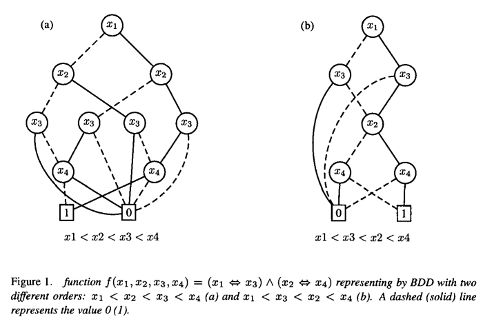
The K-terminal network reliability function can be represented by a boolean function $f$ defined as follows:
$$
\left{\begin{array}{l}
f\left(x_1, x_2, \ldots, x_m\right)=1 \text { if nodes in } K \text { are linked by edges } e_i \text { with } x_i=1 \
f\left(x_1, x_2, \ldots, x_m\right)=0 \text { otherwise }
\end{array}\right.
$$
where boolean variable $x_i$ stands for the state of the link $e_i(1 \leq i \leq m)$. For instance, the boolean formula encoded by the BDD structure in figure 3 is:
$$
x_1\left(\bar{x}_2\left(\bar{x}_3 x_4 x_5 x_6+x_3\left(\bar{x}_4 x_5 x_6+x_4\right)\right)+x_2\left(\bar{x}_4 x_5 x_6+x_4\right)\right)+\bar{x}_1 x_2\left(x_3\left(\bar{x}_4 x_5 x_6+x_4\right)+\bar{x}_3 x_5 x_6\right)
$$
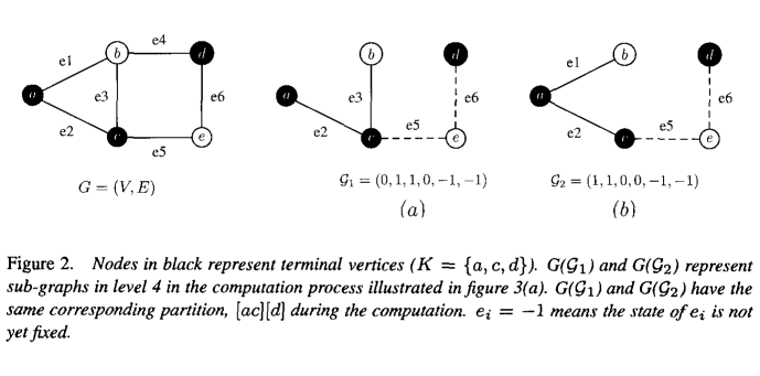
Our aim is to encode this reliability function by BDD. The algorithm is developed in Section 3.3. In figure 3(b), we explain the definition of BDD through an example of BDD representing the K-terminal reliability of network $\mathrm{G}$ (see figure

2). The BDD can represent the SDP implicitly avoiding huge storage for large number of SDP. A useful property of BDD is that all the paths from the root to the leaves are disjoint. If $f$ represents the system reliability expression, based on this property, the K-terminal network reliability $R_K$ of $G$ can be recursively evaluated by:
$$
\begin{aligned}
& \forall i \in{1, \ldots, m}: \
& R_K(p ; G)=\operatorname{Pr}(f=1) \
& R_K(p ; G)=\operatorname{Pr}\left(x_i \cdot f_{x_i=1}=1\right)+\operatorname{Pr}\left(\bar{x}i, f{x_i=0}=1\right) \
& R_K(p ; G)=p_i \cdot \operatorname{Pr}\left(f_{x_i=1}=1\right)+q_i \cdot \operatorname{Pr}\left(f_{x_i=0}=1\right) \
&
\end{aligned}
$$
with $p=\left(p_1, \ldots, p_m\right)$.
For instance, in figure $3(\mathrm{~b})$, the K-terminal network reliability is then defined as follows:
$$
R_K(p ; G)=p_1\left(q_2\left(q_3 p_4 p_5 p_6+p_3\left(q_4 p_5 p_6+p_4\right)\right)+p_2\left(q_4 p_5 p_6+p_4\right)\right)+q_1 p_2\left(p_3\left(q_4 p_5 p_6+p_4\right)+q_3 p_5 p_6\right)
$$
The next section presents our BDD-based algorithm for the K-terminal network reliability problem.

数学代写|运筹学作业代写operational research代考|Construction of the $B D D$ representing the $K$-terminal reliability function

We remind that the order of the variables is very important for BDD generation (see Section 2). Time and space complexity of BDD closely depend on variable ordering. This paper is not concerned with this kind of problem and we use a breadth-first-search (BFS) ordering.
In short, our algorithm follows three steps:

• 1 The edges are ordered by using a heuristic.
• 2 The BDD is generated to encode the network reliability. The following shows the construction of the BDD encoding the K-terminal network reliability.
• 3 From this BDD structure, we obtain the K-terminal network reliabilities (whatever $p_i, i \in[1 \ldots m]$ ) as shown in the previous section.

The top-down construction process can be represented as a binary tree such that the root corresponds to the original graph $G$ and children correspond to graphs obtained by deletion /contraction of edges. Nodes in the binary tree correspond to subgraphs of $G$. At the root, we consider the edge $e_1$, construct the subgraph $G_{-1}$, that is $G$ with $e_1$ deleted and the subgraph $G_{* 1}$ that is $G$ with $e_1$ contracted. Then at the second step, from $G_{-1}$, we construct $G_{-1-2}$ where $e_2$ is deleted and $G_{-1 * 2}$ where $e_2$ is contracted and so on from each created subgraphs until the vertices of $K$ are fully connected or at least one vertex of $K$ is disconnected. There are $2^n$ possible states and isomorphic graphs appear in the computation process. For the graph $G$ pictured in Fig. 2, its subgraphs $G_{* 1 * 2}$ and $G_{-1 * 2 * 3}$ are isomorphic. Our aim is to provide an efficient method in order to avoid redundant computation due to the appearance of isomorphic subproblems during the process. We use the method introduced by Carlier and Lucet ${ }^{15}$ for representing graph by partition which is an efficient way for solving this kind of problem. By identifying the isomorphic subgraphs an expansion tree is modified as a rooted acyclic graph which is a BDD (see figure $3(\mathrm{~b})$ ).

运筹学代考

数学代写|运筹学作业代写operational research代考|Encoding and evaluating the network reliability by $B D D$

k端网络可靠性函数可以用布尔函数$f$表示，定义如下:
$$
\left{\begin{array}{l}
f\left(x_1, x_2, \ldots, x_m\right)=1 \text { if nodes in } K \text { are linked by edges } e_i \text { with } x_i=1 \
f\left(x_1, x_2, \ldots, x_m\right)=0 \text { otherwise }
\end{array}\right.
$$
其中，布尔变量$x_i$表示链接$e_i(1 \leq i \leq m)$的状态。例如，图3中BDD结构编码的布尔公式为:
$$
x_1\left(\bar{x}_2\left(\bar{x}_3 x_4 x_5 x_6+x_3\left(\bar{x}_4 x_5 x_6+x_4\right)\right)+x_2\left(\bar{x}_4 x_5 x_6+x_4\right)\right)+\bar{x}_1 x_2\left(x_3\left(\bar{x}_4 x_5 x_6+x_4\right)+\bar{x}_3 x_5 x_6\right)
$$
我们的目标是用BDD编码这个可靠性函数。该算法将在第3.3节中开发。在图3(b)中，我们通过一个BDD代表网络k端可靠性$\mathrm{G}$的例子来解释BDD的定义(见图3)

2). BDD可以隐式地表示SDP，避免大量SDP占用巨大的存储空间。BDD的一个有用的性质是从根到叶的所有路径都是不相交的。若$f$表示系统可靠性表达式，则根据该性质，$G$的k端网络可靠性$R_K$可递归求出:
$$
\begin{aligned}
& \forall i \in{1, \ldots, m}: \
& R_K(p ; G)=\operatorname{Pr}(f=1) \
& R_K(p ; G)=\operatorname{Pr}\left(x_i \cdot f_{x_i=1}=1\right)+\operatorname{Pr}\left(\bar{x}i, f{x_i=0}=1\right) \
& R_K(p ; G)=p_i \cdot \operatorname{Pr}\left(f_{x_i=1}=1\right)+q_i \cdot \operatorname{Pr}\left(f_{x_i=0}=1\right) \
&
\end{aligned}
$$
通过$p=\left(p_1, \ldots, p_m\right)$。
例如，在图$3(\mathrm{~b})$中，则k端网络可靠性定义如下:
$$
R_K(p ; G)=p_1\left(q_2\left(q_3 p_4 p_5 p_6+p_3\left(q_4 p_5 p_6+p_4\right)\right)+p_2\left(q_4 p_5 p_6+p_4\right)\right)+q_1 p_2\left(p_3\left(q_4 p_5 p_6+p_4\right)+q_3 p_5 p_6\right)
$$
下一节介绍基于bdd的k端网络可靠性问题算法。

数学代写|运筹学作业代写operational research代考|Construction of the $B D D$ representing the $K$-terminal reliability function

我们提醒，变量的顺序对于BDD的生成非常重要(参见第2节)。BDD的时间和空间复杂性密切依赖于变量的顺序。本文不考虑这类问题，而是采用广度优先搜索(BFS)排序。
简而言之，我们的算法分为三个步骤:

边是用启发式排序的。

2生成BDD对网络可靠性进行编码。BDD编码k端网络可靠性的构造如下图所示。

从这个BDD结构中，我们得到了k端网络可靠性(无论$p_i, i \in[1 \ldots m]$)，如前一节所示。

自顶向下的构建过程可以表示为二叉树，其根对应于原始图 $G$ 子节点对应于通过删除/收缩边得到的图。二叉树中的节点对应于的子图 $G$． 在根，我们考虑边 $e_1$，构造子图 $G_{-1}$就是这样 $G$ 有 $e_1$ 删除和子图 $G_{* 1}$ 那就是 $G$ 有 $e_1$ 收缩。第二步，从 $G_{-1}$，我们构建 $G_{-1-2}$ 在哪里 $e_2$ 被删除，并且 $G_{-1 * 2}$ 在哪里 $e_2$ 从每个创建的子图，直到顶点的 $K$ 是完全连通的还是至少有一个顶点 $K$ 已断开连接。有 $2^n$ 计算过程中出现可能状态和同构图。对于这个图 $G$ 如图2所示，它的子图 $G_{* 1 * 2}$ 和 $G_{-1 * 2 * 3}$ 是同构的。我们的目标是提供一种有效的方法，以避免在此过程中由于同构子问题的出现而导致的冗余计算。我们采用了Carlier和Lucet介绍的方法 ${ }^{15}$ 用划分表示图是解决这类问题的一种有效方法。通过识别同构子图，将展开树修改为有根无环图，即BDD(见图) $3(\mathrm{~b})$ ）.

统计代写请认准statistics-lab™. statistics-lab™为您的留学生涯保驾护航。

金融工程代写

金融工程是使用数学技术来解决金融问题。金融工程使用计算机科学、统计学、经济学和应用数学领域的工具和知识来解决当前的金融问题，以及设计新的和创新的金融产品。

非参数统计代写

非参数统计指的是一种统计方法，其中不假设数据来自于由少数参数决定的规定模型；这种模型的例子包括正态分布模型和线性回归模型。

广义线性模型代考

广义线性模型（GLM）归属统计学领域，是一种应用灵活的线性回归模型。该模型允许因变量的偏差分布有除了正态分布之外的其它分布。

术语 广义线性模型（GLM）通常是指给定连续和/或分类预测因素的连续响应变量的常规线性回归模型。它包括多元线性回归，以及方差分析和方差分析（仅含固定效应）。

有限元方法代写

有限元方法（FEM）是一种流行的方法，用于数值解决工程和数学建模中出现的微分方程。典型的问题领域包括结构分析、传热、流体流动、质量运输和电磁势等传统领域。

有限元是一种通用的数值方法，用于解决两个或三个空间变量的偏微分方程（即一些边界值问题）。为了解决一个问题，有限元将一个大系统细分为更小、更简单的部分，称为有限元。这是通过在空间维度上的特定空间离散化来实现的，它是通过构建对象的网格来实现的：用于求解的数值域，它有有限数量的点。边界值问题的有限元方法表述最终导致一个代数方程组。该方法在域上对未知函数进行逼近。[1] 然后将模拟这些有限元的简单方程组合成一个更大的方程系统，以模拟整个问题。然后，有限元通过变化微积分使相关的误差函数最小化来逼近一个解决方案。

tatistics-lab作为专业的留学生服务机构，多年来已为美国、英国、加拿大、澳洲等留学热门地的学生提供专业的学术服务，包括但不限于Essay代写，Assignment代写，Dissertation代写，Report代写，小组作业代写，Proposal代写，Paper代写，Presentation代写，计算机作业代写，论文修改和润色，网课代做，exam代考等等。写作范围涵盖高中，本科，研究生等海外留学全阶段，辐射金融，经济学，会计学，审计学，管理学等全球99%专业科目。写作团队既有专业英语母语作者，也有海外名校硕博留学生，每位写作老师都拥有过硬的语言能力，专业的学科背景和学术写作经验。我们承诺100%原创，100%专业，100%准时，100%满意。

随机分析代写

随机微积分是数学的一个分支，对随机过程进行操作。它允许为随机过程的积分定义一个关于随机过程的一致的积分理论。这个领域是由日本数学家伊藤清在第二次世界大战期间创建并开始的。

时间序列分析代写

随机过程，是依赖于参数的一组随机变量的全体，参数通常是时间。 随机变量是随机现象的数量表现，其时间序列是一组按照时间发生先后顺序进行排列的数据点序列。通常一组时间序列的时间间隔为一恒定值（如1秒，5分钟，12小时，7天，1年），因此时间序列可以作为离散时间数据进行分析处理。研究时间序列数据的意义在于现实中，往往需要研究某个事物其随时间发展变化的规律。这就需要通过研究该事物过去发展的历史记录，以得到其自身发展的规律。

回归分析代写

多元回归分析渐进（Multiple Regression Analysis Asymptotics）属于计量经济学领域，主要是一种数学上的统计分析方法，可以分析复杂情况下各影响因素的数学关系，在自然科学、社会和经济学等多个领域内应用广泛。

MATLAB代写

MATLAB 是一种用于技术计算的高性能语言。它将计算、可视化和编程集成在一个易于使用的环境中，其中问题和解决方案以熟悉的数学符号表示。典型用途包括：数学和计算算法开发建模、仿真和原型制作数据分析、探索和可视化科学和工程图形应用程序开发，包括图形用户界面构建MATLAB 是一个交互式系统，其基本数据元素是一个不需要维度的数组。这使您可以解决许多技术计算问题，尤其是那些具有矩阵和向量公式的问题，而只需用 C 或 Fortran 等标量非交互式语言编写程序所需的时间的一小部分。MATLAB 名称代表矩阵实验室。MATLAB 最初的编写目的是提供对由 LINPACK 和 EISPACK 项目开发的矩阵软件的轻松访问，这两个项目共同代表了矩阵计算软件的最新技术。MATLAB 经过多年的发展，得到了许多用户的投入。在大学环境中，它是数学、工程和科学入门和高级课程的标准教学工具。在工业领域，MATLAB 是高效研究、开发和分析的首选工具。MATLAB 具有一系列称为工具箱的特定于应用程序的解决方案。对于大多数 MATLAB 用户来说非常重要，工具箱允许您学习和应用专业技术。工具箱是 MATLAB 函数（M 文件）的综合集合，可扩展 MATLAB 环境以解决特定类别的问题。可用工具箱的领域包括信号处理、控制系统、神经网络、模糊逻辑、小波、仿真等。

R语言代写	问卷设计与分析代写
PYTHON代写	回归分析与线性模型代写
MATLAB代写	方差分析与试验设计代写
STATA代写	机器学习/统计学习代写
SPSS代写	计量经济学代写
EVIEWS代写	时间序列分析代写
EXCEL代写	深度学习代写
SQL代写	各种数据建模与可视化代写

如果你也在 怎样代写运筹学Operations Research 这个学科遇到相关的难题，请随时右上角联系我们的24/7代写客服。运筹学Operations Research为管理者、工程师和任何有更好解决方案的实践者提供更好的解决方案。这门科学诞生于第二次世界大战期间。虽然它最初用于军事行动，但它的应用以某种形式扩展到地球上的任何领域。

运筹学Operations Research是将科学方法应用于解决复杂问题，指导和管理工业、商业、政府和国防中由人、机器、材料和资金组成的大型系统。独特的方法是开发一个系统的科学模型，包括诸如变化和风险等因素的测量，以此来预测和比较不同决策、战略或控制的结果。其目的是帮助管理层科学地确定其政策和行动。

statistics-lab™ 为您的留学生涯保驾护航 在代写运筹学operational research方面已经树立了自己的口碑, 保证靠谱, 高质且原创的统计Statistics代写服务。我们的专家在代写运筹学operational research代写方面经验极为丰富，各种代写运筹学operational research相关的作业也就用不着说。

数学代写|运筹学作业代写operational research代考|Binary Decision Diagram (BDD)

Akers ${ }^1$ first introduced BDD for representing boolean function. Bryant popularized the use of BDD by introducing a set of algorithms for efficient construction and manipulation of the BDD structure ${ }^2$. Nowadays, BDD are used in a wide range of area, including hardware synthesis and verification, model checking and protocol validation. Their use in the reliability analysis framework has been introduced by Madre and Coudert ${ }^5 4$ and developped by Odeh ${ }^6$ and Rauzy ${ }^3$. Sekine and Imai have introduced the BDD structure in network reliability ${ }^{10} 11$. The BDD structure provides compact representations of boolean expressions. A BDD is a directed acyclic graph (DAG) based on Shannon’s decomposition. The Shannon’s decomposition for a boolean function $f$ is defined as follows:
$$
f=x f_{x=1}+\bar{x} f_{x=0}
$$
where $x$ is one of decision variables and $f_{x=i}$ is the boolean function $f$ evaluated at $x=i$.

The graph has two sink nodes labeled with 0 and 1 representing the two corresponding constant expressions. Each internal node is labeled with a boolean variable $x$ and has two out-edges called 0 -edge and 1-edge. The node linked by 1-edge represents the boolean expression when $x=1$, i.e. $f_{x=1}$ while the node linked by 0 -edge represents the boolean expression when $x=0$, i.e. $f_{x=0}$. An ordered binary decision diagram (OBDD) is a BDD where variables are ordered according to a known total ordering and every path visits variables in an ascending order. Afterwards, BDDs will be considered as ordered. Leaves of the BDD give the value of $f$ for the assignment corresponding to a path from the root to the leaf.

The size of a BDD structure (the number of nodes) depends critically on the chosen variable ordering. Figure 1 shows the effect of the variable ordering on the BDD size. If we consider the expression $\left(x_1 \Leftrightarrow x_3\right) \wedge\left(x_2 \Leftrightarrow x_4\right)$ the resulting BDD using the ordering $x_1<x_2<x_3<x_4$ consists of 11 nodes (figure 1(a)) and not 8 nodes as for the ordering $x_1<x_3<x_2<x_4$ (figure 1(b)). Finding an ordering that minimizes the size of BDD is also a NP-complete problem ${ }^7$. Several heuristics relying on different principles have been proposed in many domains. However, they both try to put close in the order the variables that are close in the formula as illustrated in figure 1 .

数学代写|运筹学作业代写operational research代考|Definitions and notations

The K-terminal reliability computation is the most general network reliability problem found in the literature. It consists in evaluating the probability that net work components of a specified subset $K$ remain connected when the components are subject to failure.

Our network model is an undirected stochastic graph $G=(V, E)$, with $V$ its set of vertex (representing workstations, servers, routers …) and $E \subseteq V \times V$ its set of edges (representing the links between these nodes). Each edge $e_i$ of the stochastic graph is subject to failure with known probability $q_i$. We denote $p_i=1-q_i$ the probability that edge $e_i$ functions, and assume that all the failure events are statistically independent. In the following, we consider the vertices as perfect, but the proposed algorithms are still functioning for such problem. In classical enumerative method, all the states of the graph are generated, evaluated as a fail state or a functioning state, and then probabilistic methods are used for computing the associated reliability. So, as there are two states for each edge, there are $2^m$ (with $m=|E|$ ) possible states for the graph. A state $\mathcal{G}$ of the stochastic graph $G$ is denoted by $\left(x_1, x_2 \ldots, x_m\right)$ where $x_i$ stands for the state of edge $e_i$, i.e. $x_i=0$ when edge $e_i$ fails and $x_i=1$ when it functions. The associated probability of $\mathcal{G}$ is defined as:
$$
\operatorname{Pr}(\mathcal{G})=\prod_{i=1}^m\left(x_i \cdot p_i+\left(1-x_i\right) \cdot q_i\right)
$$
At each state $\mathcal{G}$ is associated a partial graph $G(\mathcal{G})=\left(V, E^{\prime}\right)$ such that $e_i \in E^{\prime}$ if and only if $e_i \in E$ and $x_i=1$. A path is defined as a set of edges such that if these edges are all up, the system is up. A path is minimal if it has no proper subpaths. We define a subset of the nodes $K \subseteq V$ to be the “terminals” (with $2 \leq|K| \leq|V|)$. If $|K|=2$ this problem is well-known as the 2 -terminal reliability problem and if $|K|=|V|$ it deals with the all-terminal reliability problem. The terminal nodes are essential to the system function and have to communicate with each other, i.e. the network is up if and only if there exists at least one path made of functioning edges linking nodes in $K$. The K-terminal reliability, denoted by $R_K(p ; G)\left(p=\left(p_1, \ldots, p_m\right)\right)$, is the probability that all vertices in $K$ are connected and can be defined as follows:
$$
R_K(p ; G)=\sum_{\text {K-nodes are connected by working links in } G(\mathcal{G})} \operatorname{Pr}(\mathcal{G})
$$

运筹学代考

数学代写|运筹学作业代写operational research代考|Binary Decision Diagram (BDD)

Akers ${ }^1$首先引入BDD来表示布尔函数。Bryant通过引入一套有效构建和操作BDD结构${ }^2$的算法，推广了BDD的使用。目前，BDD已广泛应用于硬件综合与验证、模型检验和协议验证等领域。它们在可靠性分析框架中的使用已由Madre和Coudert ${ }^5 4$引入，并由Odeh ${ }^6$和Rauzy ${ }^3$开发。Sekine和Imai在网络可靠性方面引入了BDD结构${ }^{10} 11$。BDD结构提供了布尔表达式的紧凑表示。BDD是基于香农分解的有向无环图(DAG)。布尔函数$f$的香农分解定义如下:
$$
f=x f_{x=1}+\bar{x} f_{x=0}
$$
其中$x$是一个决策变量，$f_{x=i}$是布尔函数$f$，在$x=i$处求值。

该图有两个标记为0和1的汇聚节点，表示两个对应的常量表达式。每个内部节点都用布尔变量$x$标记，并有两个外边，分别称为0边和1边。1边连接的节点表示$x=1$时的布尔表达式，即$f_{x=1}$; 0边连接的节点表示$x=0$时的布尔表达式，即$f_{x=0}$。有序二进制决策图(OBDD)是一种BDD，其中变量根据已知的总排序排序，并且每个路径以升序访问变量。之后，bdd将被视为订购。BDD的叶节点为从根节点到叶节点的路径对应的赋值提供$f$。

BDD结构的大小(节点数量)主要取决于所选择的变量排序。图1显示了变量排序对BDD大小的影响。如果我们考虑表达式$\left(x_1 \Leftrightarrow x_3\right) \wedge\left(x_2 \Leftrightarrow x_4\right)$，那么使用顺序$x_1<x_2<x_3<x_4$得到的BDD由11个节点组成(图1(a))，而不是顺序$x_1<x_3<x_2<x_4$的8个节点(图1(b))。找到最小化BDD大小的排序也是一个np完全问题${ }^7$。许多领域都提出了基于不同原理的启发式方法。然而，它们都试图按照公式中接近的变量的顺序排列，如图1所示。

数学代写|运筹学作业代写operational research代考|Definitions and notations

k端可靠性计算是文献中发现的最普遍的网络可靠性问题。它包括评估特定子集$K$的网络组件在组件发生故障时保持连接的概率。

我们的网络模型是一个无向随机图$G=(V, E)$，其中$V$是一组顶点(代表工作站、服务器、路由器……)，$E \subseteq V \times V$是一组边(代表这些节点之间的链接)。随机图的每条边$e_i$都以已知的概率$q_i$失效。我们表示$p_i=1-q_i$边$e_i$函数的概率，并假设所有故障事件在统计上是独立的。在下面，我们认为顶点是完美的，但所提出的算法仍然适用于此类问题。在经典的枚举方法中，首先生成图的所有状态，并将其评估为失效状态或功能状态，然后使用概率方法计算相关的可靠度。因此，由于每条边都有两种状态，因此图有$2^m$(与$m=|E|$)可能的状态。随机图$G$的状态$\mathcal{G}$用$\left(x_1, x_2 \ldots, x_m\right)$表示，其中$x_i$表示边$e_i$的状态，即，当边$e_i$失效时为$x_i=0$，当边起作用时为$x_i=1$。$\mathcal{G}$的关联概率定义为:
$$
\operatorname{Pr}(\mathcal{G})=\prod_{i=1}^m\left(x_i \cdot p_i+\left(1-x_i\right) \cdot q_i\right)
$$
在每个状态$\mathcal{G}$都关联一个偏图$G(\mathcal{G})=\left(V, E^{\prime}\right)$，使得$e_i \in E^{\prime}$当且仅当$e_i \in E$和$x_i=1$。路径被定义为一组边，如果这些边都是上的，那么这个系统就是上的。如果一条路径没有合适的子路径，那么它就是最小路径。我们将节点的子集$K \subseteq V$定义为“终端”(使用$2 \leq|K| \leq|V|)$)。如果$|K|=2$这个问题是众所周知的2终端可靠性问题，如果$|K|=|V|$它处理的是全终端可靠性问题。终端节点对系统功能至关重要，并且必须相互通信，即当且仅当存在至少一条由连接$K$中的节点的功能边组成的路径时，网络才会启动。k端可靠度，用$R_K(p ; G)\left(p=\left(p_1, \ldots, p_m\right)\right)$表示，是$K$中所有顶点连通的概率，定义如下:
$$
R_K(p ; G)=\sum_{\text {K-nodes are connected by working links in } G(\mathcal{G})} \operatorname{Pr}(\mathcal{G})
$$

统计代写请认准statistics-lab™. statistics-lab™为您的留学生涯保驾护航。

金融工程代写

金融工程是使用数学技术来解决金融问题。金融工程使用计算机科学、统计学、经济学和应用数学领域的工具和知识来解决当前的金融问题，以及设计新的和创新的金融产品。

非参数统计代写

非参数统计指的是一种统计方法，其中不假设数据来自于由少数参数决定的规定模型；这种模型的例子包括正态分布模型和线性回归模型。

广义线性模型代考

广义线性模型（GLM）归属统计学领域，是一种应用灵活的线性回归模型。该模型允许因变量的偏差分布有除了正态分布之外的其它分布。

术语 广义线性模型（GLM）通常是指给定连续和/或分类预测因素的连续响应变量的常规线性回归模型。它包括多元线性回归，以及方差分析和方差分析（仅含固定效应）。

有限元方法代写

有限元方法（FEM）是一种流行的方法，用于数值解决工程和数学建模中出现的微分方程。典型的问题领域包括结构分析、传热、流体流动、质量运输和电磁势等传统领域。

有限元是一种通用的数值方法，用于解决两个或三个空间变量的偏微分方程（即一些边界值问题）。为了解决一个问题，有限元将一个大系统细分为更小、更简单的部分，称为有限元。这是通过在空间维度上的特定空间离散化来实现的，它是通过构建对象的网格来实现的：用于求解的数值域，它有有限数量的点。边界值问题的有限元方法表述最终导致一个代数方程组。该方法在域上对未知函数进行逼近。[1] 然后将模拟这些有限元的简单方程组合成一个更大的方程系统，以模拟整个问题。然后，有限元通过变化微积分使相关的误差函数最小化来逼近一个解决方案。

tatistics-lab作为专业的留学生服务机构，多年来已为美国、英国、加拿大、澳洲等留学热门地的学生提供专业的学术服务，包括但不限于Essay代写，Assignment代写，Dissertation代写，Report代写，小组作业代写，Proposal代写，Paper代写，Presentation代写，计算机作业代写，论文修改和润色，网课代做，exam代考等等。写作范围涵盖高中，本科，研究生等海外留学全阶段，辐射金融，经济学，会计学，审计学，管理学等全球99%专业科目。写作团队既有专业英语母语作者，也有海外名校硕博留学生，每位写作老师都拥有过硬的语言能力，专业的学科背景和学术写作经验。我们承诺100%原创，100%专业，100%准时，100%满意。

随机分析代写

随机微积分是数学的一个分支，对随机过程进行操作。它允许为随机过程的积分定义一个关于随机过程的一致的积分理论。这个领域是由日本数学家伊藤清在第二次世界大战期间创建并开始的。

时间序列分析代写

随机过程，是依赖于参数的一组随机变量的全体，参数通常是时间。 随机变量是随机现象的数量表现，其时间序列是一组按照时间发生先后顺序进行排列的数据点序列。通常一组时间序列的时间间隔为一恒定值（如1秒，5分钟，12小时，7天，1年），因此时间序列可以作为离散时间数据进行分析处理。研究时间序列数据的意义在于现实中，往往需要研究某个事物其随时间发展变化的规律。这就需要通过研究该事物过去发展的历史记录，以得到其自身发展的规律。

回归分析代写

多元回归分析渐进（Multiple Regression Analysis Asymptotics）属于计量经济学领域，主要是一种数学上的统计分析方法，可以分析复杂情况下各影响因素的数学关系，在自然科学、社会和经济学等多个领域内应用广泛。

MATLAB代写

MATLAB 是一种用于技术计算的高性能语言。它将计算、可视化和编程集成在一个易于使用的环境中，其中问题和解决方案以熟悉的数学符号表示。典型用途包括：数学和计算算法开发建模、仿真和原型制作数据分析、探索和可视化科学和工程图形应用程序开发，包括图形用户界面构建MATLAB 是一个交互式系统，其基本数据元素是一个不需要维度的数组。这使您可以解决许多技术计算问题，尤其是那些具有矩阵和向量公式的问题，而只需用 C 或 Fortran 等标量非交互式语言编写程序所需的时间的一小部分。MATLAB 名称代表矩阵实验室。MATLAB 最初的编写目的是提供对由 LINPACK 和 EISPACK 项目开发的矩阵软件的轻松访问，这两个项目共同代表了矩阵计算软件的最新技术。MATLAB 经过多年的发展，得到了许多用户的投入。在大学环境中，它是数学、工程和科学入门和高级课程的标准教学工具。在工业领域，MATLAB 是高效研究、开发和分析的首选工具。MATLAB 具有一系列称为工具箱的特定于应用程序的解决方案。对于大多数 MATLAB 用户来说非常重要，工具箱允许您学习和应用专业技术。工具箱是 MATLAB 函数（M 文件）的综合集合，可扩展 MATLAB 环境以解决特定类别的问题。可用工具箱的领域包括信号处理、控制系统、神经网络、模糊逻辑、小波、仿真等。

R语言代写	问卷设计与分析代写
PYTHON代写	回归分析与线性模型代写
MATLAB代写	方差分析与试验设计代写
STATA代写	机器学习/统计学习代写
SPSS代写	计量经济学代写
EVIEWS代写	时间序列分析代写
EXCEL代写	深度学习代写
SQL代写	各种数据建模与可视化代写

如果你也在 怎样代写运筹学Operations Research 这个学科遇到相关的难题，请随时右上角联系我们的24/7代写客服。运筹学Operations Research为管理者、工程师和任何有更好解决方案的实践者提供更好的解决方案。这门科学诞生于第二次世界大战期间。虽然它最初用于军事行动，但它的应用以某种形式扩展到地球上的任何领域。

运筹学Operations Research是将科学方法应用于解决复杂问题，指导和管理工业、商业、政府和国防中由人、机器、材料和资金组成的大型系统。独特的方法是开发一个系统的科学模型，包括诸如变化和风险等因素的测量，以此来预测和比较不同决策、战略或控制的结果。其目的是帮助管理层科学地确定其政策和行动。

statistics-lab™ 为您的留学生涯保驾护航 在代写运筹学operational research方面已经树立了自己的口碑, 保证靠谱, 高质且原创的统计Statistics代写服务。我们的专家在代写运筹学operational research代写方面经验极为丰富，各种代写运筹学operational research相关的作业也就用不着说。

数学代写|运筹学作业代写operational research代考|The Markov Chain Monte Carlo Method

In this section, we present the utilisation of Markov chain Monte Carlo method (see Chen, Shao and Ibrahim $^6$ ) for estimating $\tau$ and the parameters of the initial lifetime distribution. To simplify the matter, we assume that the first two lifetimes are observed and the repair type is known to be WTNBTU.

The McMC methods enable us to simulate a Markov chain whose stationary distribution is our “target” distribution, for instance, the posterior distribution of the parameter of interest. We will use the Gibbs sampler which is one of the McMC methods. Under our model, the Gibbs sampler can be described as follows:
(1) Start with an arbitrary initial vector $\theta^{(0)}=\left(\tau^{(0)}, \alpha^{(0)}, \beta^{(0)}\right)$ and set $k=0$.
(2) Sample $\tau^{(k+1)}$ from $\pi\left(\tau \mid \alpha^{(k)}, \beta^{(k)}, x_1, x_2\right)$.
(3) Sample $\alpha^{(k+1)}$ from $\pi\left(\alpha \mid \tau^{(k+1)}, \beta^{(k)}, x_1, x_2\right)$.
(4) Sample $\beta^{(k+1)}$ from $\pi\left(\beta \mid \tau^{(k+1)}, \alpha^{(k+1)}, x_1, x_2\right)$.
(5) Set $\theta^{(k+1)}=\left(\tau^{(k+1)}, \alpha^{(k+1)}, \beta^{(k+1)}\right)$ and $k=k+1$. Go back to the second step.

Here, $\pi(\cdot \mid \cdot)$ denotes a full conditional density function. For instance,
$$
\pi\left(\tau \mid \alpha^{(k)}, \beta^{(k)}, x_1, x_2\right)
$$

denotes the conditional density function of $\tau$ given current values of all the other parameters as well as two failure times. One can obtain each full conditional density up to a proportionality constant as follows by, firstly, obtaining the joint density function of all the parameters and failure times, i.e.,
$$
L\left(\tau, \alpha, \beta \mid x_1, x_2\right) \pi(\tau) \pi(\alpha) \pi(\beta),
$$
and then viewing (5) as a function of the parameter of interest. With our model assumptions, direct sampling from each full conditional cannot be easily done due to the indexing parameter $\tau$ (see Gilks ${ }^5$ ). MetropolisHastings algorithms (see Metropolis et al. ${ }^8$ and Hastings ${ }^9$ ) can be used to draw samples from the full conditionals. The Metropolis-Hastings method is an McMC methods that includes the Gibbs sampler as a special case (see Chib and Greenberg $\left.{ }^7\right)$. Under certain regularity conditions, for sufficiently large $k,\left{\theta^{(m)}: k \leq m \leq(k+n-1)\right}$ is approximately an i.i.d. sample of size $n$ from the posterior distribution of $\tau, \alpha, \beta$ given $\left(x_1, x_2\right)$. Numerical examples will illustrate our approach.

数学代写|运筹学作业代写operational research代考|Example

In this section we will reconsider the example discussed in ${ }^{12}$ and summarize the findings on the estimation of $\tau$ using maximum likelihood approach. Further, we will estimate $\tau$ from Bayesian prospective and compare the results of the two approaches. As in ${ }^{12}$, we will restrict our attention on the comparison of two consecutive lifetime distributions by using corresponding failure rate functions.
We will begin with the following assumptions:

• The item, $S$, subject to failures/repairs, has a complex structure comprising $m$ subsystems, i.e., $S=\left{S_1, S_2, \ldots S_m\right}$.
• A failure of a particular subsystem requires a type of repair which is known in advance.

For example, let us consider a car. If the failure affects the tires of a car (say subsystem $S_1$ ), usually a complete repair is required. On the other hand, if the charging system of the car (say subsystem $S_2$ ) fails, worse than new, better than used (WTNBTU) repair is performed. The information on warranty failures and repairs is usually strictly confidential and it is very difficult to obtain real warranty data even for research purposes. For this reason we demonstrate how one might estimate the parameters of our model using simulated data.

运筹学代考

数学代写|运筹学作业代写operational research代考|The Markov Chain Monte Carlo Method

在本节中，我们提出利用马尔可夫链蒙特卡罗方法(见Chen, Shao和Ibrahim $^6$)来估计$\tau$和初始寿命分布的参数。为了简化问题，我们假设观察到前两个生命周期，并且已知修复类型为WTNBTU。

McMC方法使我们能够模拟一个马尔可夫链，其平稳分布是我们的“目标”分布，例如，感兴趣的参数的后验分布。我们将使用Gibbs采样器，这是McMC方法之一。在我们的模型下，吉布斯采样器可以描述为:
(1)从任意初始向量$\theta^{(0)}=\left(\tau^{(0)}, \alpha^{(0)}, \beta^{(0)}\right)$开始，设置$k=0$。
(2)样本$\tau^{(k+1)}$来自$\pi\left(\tau \mid \alpha^{(k)}, \beta^{(k)}, x_1, x_2\right)$。
(3)从$\pi\left(\alpha \mid \tau^{(k+1)}, \beta^{(k)}, x_1, x_2\right)$获取$\alpha^{(k+1)}$样本。
(4)从$\pi\left(\beta \mid \tau^{(k+1)}, \alpha^{(k+1)}, x_1, x_2\right)$获取$\beta^{(k+1)}$样本。
(5)设置$\theta^{(k+1)}=\left(\tau^{(k+1)}, \alpha^{(k+1)}, \beta^{(k+1)}\right)$和$k=k+1$。回到第二步。

这里，$\pi(\cdot \mid \cdot)$表示一个完整的条件密度函数。例如，
$$
\pi\left(\tau \mid \alpha^{(k)}, \beta^{(k)}, x_1, x_2\right)
$$

表示在给定所有其他参数的电流值和两次失效次数时$\tau$的条件密度函数。我们可以得到每一个达到比例常数的满条件密度，方法如下:首先，得到所有参数和失效时间的联合密度函数，即
$$
L\left(\tau, \alpha, \beta \mid x_1, x_2\right) \pi(\tau) \pi(\alpha) \pi(\beta),
$$
然后将(5)作为感兴趣参数的函数。使用我们的模型假设，由于索引参数$\tau$(参见Gilks ${ }^5$)，从每个完整条件中直接抽样不容易完成。MetropolisHastings算法(参见Metropolis等人${ }^8$和Hastings ${ }^9$)可用于从完整条件中提取样本。Metropolis-Hastings方法是一种McMC方法，其中包括吉布斯采样器作为一种特殊情况(参见Chib和Greenberg $\left.{ }^7\right)$)。在一定的正则性条件下，对于足够大的$k,\left{\theta^{(m)}: k \leq m \leq(k+n-1)\right}$近似为一个大小为$n$的i.i.d样本，来自于$\tau, \alpha, \beta$给定$\left(x_1, x_2\right)$的后验分布。数值例子将说明我们的方法。

数学代写|运筹学作业代写operational research代考|Example

在本节中，我们将重新考虑${ }^{12}$中讨论的示例，并总结使用最大似然方法估计$\tau$的结果。进一步，我们将从贝叶斯的角度估计$\tau$，并比较两种方法的结果。与${ }^{12}$一样，我们将通过使用相应的故障率函数将注意力限制在两个连续寿命分布的比较上。
我们将从以下假设开始:

项目$S$有故障/修理，结构复杂，包括$m$个子系统，即$S=\left{S_1, S_2, \ldots S_m\right}$。

一个特定子系统的故障需要一种预先知道的修复方法。

例如，让我们考虑一辆汽车。如果故障影响到汽车的轮胎(比如子系统$S_1$)，通常需要进行彻底的修理。另一方面，如果汽车的充电系统(例如子系统$S_2$)发生故障，则进行比新更坏，比旧更好(WTNBTU)的维修。关于保修故障和维修的信息通常是严格保密的，即使是为了研究目的，也很难获得真实的保修数据。出于这个原因，我们演示了如何使用模拟数据估计模型的参数。

统计代写请认准statistics-lab™. statistics-lab™为您的留学生涯保驾护航。

金融工程代写

金融工程是使用数学技术来解决金融问题。金融工程使用计算机科学、统计学、经济学和应用数学领域的工具和知识来解决当前的金融问题，以及设计新的和创新的金融产品。

非参数统计代写

非参数统计指的是一种统计方法，其中不假设数据来自于由少数参数决定的规定模型；这种模型的例子包括正态分布模型和线性回归模型。

广义线性模型代考

广义线性模型（GLM）归属统计学领域，是一种应用灵活的线性回归模型。该模型允许因变量的偏差分布有除了正态分布之外的其它分布。

术语 广义线性模型（GLM）通常是指给定连续和/或分类预测因素的连续响应变量的常规线性回归模型。它包括多元线性回归，以及方差分析和方差分析（仅含固定效应）。

有限元方法代写

有限元方法（FEM）是一种流行的方法，用于数值解决工程和数学建模中出现的微分方程。典型的问题领域包括结构分析、传热、流体流动、质量运输和电磁势等传统领域。

有限元是一种通用的数值方法，用于解决两个或三个空间变量的偏微分方程（即一些边界值问题）。为了解决一个问题，有限元将一个大系统细分为更小、更简单的部分，称为有限元。这是通过在空间维度上的特定空间离散化来实现的，它是通过构建对象的网格来实现的：用于求解的数值域，它有有限数量的点。边界值问题的有限元方法表述最终导致一个代数方程组。该方法在域上对未知函数进行逼近。[1] 然后将模拟这些有限元的简单方程组合成一个更大的方程系统，以模拟整个问题。然后，有限元通过变化微积分使相关的误差函数最小化来逼近一个解决方案。

tatistics-lab作为专业的留学生服务机构，多年来已为美国、英国、加拿大、澳洲等留学热门地的学生提供专业的学术服务，包括但不限于Essay代写，Assignment代写，Dissertation代写，Report代写，小组作业代写，Proposal代写，Paper代写，Presentation代写，计算机作业代写，论文修改和润色，网课代做，exam代考等等。写作范围涵盖高中，本科，研究生等海外留学全阶段，辐射金融，经济学，会计学，审计学，管理学等全球99%专业科目。写作团队既有专业英语母语作者，也有海外名校硕博留学生，每位写作老师都拥有过硬的语言能力，专业的学科背景和学术写作经验。我们承诺100%原创，100%专业，100%准时，100%满意。

随机分析代写

随机微积分是数学的一个分支，对随机过程进行操作。它允许为随机过程的积分定义一个关于随机过程的一致的积分理论。这个领域是由日本数学家伊藤清在第二次世界大战期间创建并开始的。

时间序列分析代写

随机过程，是依赖于参数的一组随机变量的全体，参数通常是时间。 随机变量是随机现象的数量表现，其时间序列是一组按照时间发生先后顺序进行排列的数据点序列。通常一组时间序列的时间间隔为一恒定值（如1秒，5分钟，12小时，7天，1年），因此时间序列可以作为离散时间数据进行分析处理。研究时间序列数据的意义在于现实中，往往需要研究某个事物其随时间发展变化的规律。这就需要通过研究该事物过去发展的历史记录，以得到其自身发展的规律。

回归分析代写

多元回归分析渐进（Multiple Regression Analysis Asymptotics）属于计量经济学领域，主要是一种数学上的统计分析方法，可以分析复杂情况下各影响因素的数学关系，在自然科学、社会和经济学等多个领域内应用广泛。

MATLAB代写

MATLAB 是一种用于技术计算的高性能语言。它将计算、可视化和编程集成在一个易于使用的环境中，其中问题和解决方案以熟悉的数学符号表示。典型用途包括：数学和计算算法开发建模、仿真和原型制作数据分析、探索和可视化科学和工程图形应用程序开发，包括图形用户界面构建MATLAB 是一个交互式系统，其基本数据元素是一个不需要维度的数组。这使您可以解决许多技术计算问题，尤其是那些具有矩阵和向量公式的问题，而只需用 C 或 Fortran 等标量非交互式语言编写程序所需的时间的一小部分。MATLAB 名称代表矩阵实验室。MATLAB 最初的编写目的是提供对由 LINPACK 和 EISPACK 项目开发的矩阵软件的轻松访问，这两个项目共同代表了矩阵计算软件的最新技术。MATLAB 经过多年的发展，得到了许多用户的投入。在大学环境中，它是数学、工程和科学入门和高级课程的标准教学工具。在工业领域，MATLAB 是高效研究、开发和分析的首选工具。MATLAB 具有一系列称为工具箱的特定于应用程序的解决方案。对于大多数 MATLAB 用户来说非常重要，工具箱允许您学习和应用专业技术。工具箱是 MATLAB 函数（M 文件）的综合集合，可扩展 MATLAB 环境以解决特定类别的问题。可用工具箱的领域包括信号处理、控制系统、神经网络、模糊逻辑、小波、仿真等。

R语言代写	问卷设计与分析代写
PYTHON代写	回归分析与线性模型代写
MATLAB代写	方差分析与试验设计代写
STATA代写	机器学习/统计学习代写
SPSS代写	计量经济学代写
EVIEWS代写	时间序列分析代写
EXCEL代写	深度学习代写
SQL代写	各种数据建模与可视化代写