Math5845 - 统计代写答疑辅导

标签： Math5845

统计代写|时间序列分析代写Time-Series Analysis代考|STAT4025

Posted on 2022年6月9日2022年6月9日 by statistics-lab

如果你也在怎样代写时间序列分析Time-Series Analysis这个学科遇到相关的难题，请随时右上角联系我们的24/7代写客服。

时间序列分析是分析在一个时间间隔内收集的一系列数据点的具体方式。在时间序列分析中，分析人员在设定的时间段内以一致的时间间隔记录数据点，而不仅仅是间歇性或随机地记录数据点。

statistics-lab™ 为您的留学生涯保驾护航在代写时间序列分析Time-Series Analysis方面已经树立了自己的口碑, 保证靠谱, 高质且原创的统计Statistics代写服务。我们的专家在代写时间序列分析Time-Series Analysis代写方面经验极为丰富，各种代写时间序列分析Time-Series Analysis相关的作业也就用不着说。

我们提供的时间序列分析Time-Series Analysis及其相关学科的代写，服务范围广, 其中包括但不限于:

Statistical Inference 统计推断
Statistical Computing 统计计算
Advanced Probability Theory 高等概率论
Advanced Mathematical Statistics 高等数理统计学
(Generalized) Linear Models 广义线性模型
Statistical Machine Learning 统计机器学习
Longitudinal Data Analysis 纵向数据分析
Foundations of Data Science 数据科学基础

统计代写|时间序列分析代写Time-Series Analysis代考|STAT4025

统计代写|时间序列分析代写Time-Series Analysis代考|Quasi-Biennial Oscillation

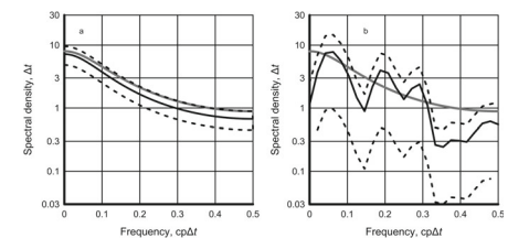
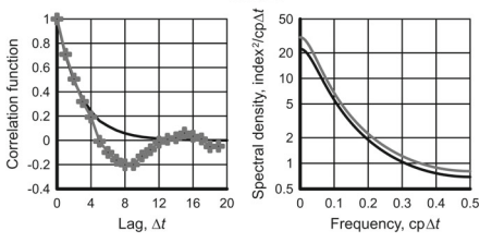
The Quasi-Biennial Oscillation will be discussed here at $\Delta t=1$ month. The time series used for this example is $\mathrm{QBO}$ at the atmospheric pressure level $20 \mathrm{hPa}$, which corresponds to the altitude of about $26 \mathrm{~km}$ above mean sea level (Fig. $6.5 \mathrm{a}$ and $# 2$ in Appendix). The spectral density estimate is shown in Fig. $6.5 \mathrm{~b}$ with the frequency axis given in a linear scale.

At the time when this text was being written, monthly observations of QBO were available from January 1953 through April of 2019 . The test extrapolation for the entire 2018 and the next six months of 2019, from May through November, which have been added in December 2019, is based upon the part of the time series that ends in December $2017(N=780)$.

The optimal, according to three of the five order selection criteria used here, is the AR model of order $p=10$ :
$$
x_{t}=\varphi_{1} x_{t-1}+\varphi_{2} x_{t-2}+\cdots+\varphi_{10} x_{t-10}+a_{t} .
$$
It means that the extrapolation equation is
$$
\hat{x}{t}(\tau)=\varphi{1} \hat{x}{t}(\tau-1)+\varphi{2} \hat{x}{t}(\tau-2)+\cdots+\varphi{10} \hat{x}{t}(\tau-10) $$ The white noise variance corresponding to the $\operatorname{AR}(10)$ model is $\sigma{a}^{2} \approx 21(\mathrm{~m} / \mathrm{s})^{2}$ while the total variance of wind speed at $20 \mathrm{hPa}$ is $\sigma_{x}^{2} \approx 389(\mathrm{~m} / \mathrm{s})^{2}$. Therefore, the predictability criterion $\rho(1) \approx 0.05$ and the correlation coefficient $(6.13)$ between the unknown true and predicted values of wind speed at lead time $\tau=1$ month is $0.97$. As seen from Fig. 6.6, the statistical predictability of $\mathrm{QBO}$ at the $20 \mathrm{hPa}$ level described with the predictability criteria $r_{e}(\tau)$ and $\rho(\tau)$ is quite high.

The results of prediction test with the initial time in December 2017 (Fig. 6.7a) show that the AR method of extrapolation is working quite well with this time series: 19 of the 20 monthly forecasts stay within the $90 \%$ confidence limits. More predictions are given from December 2018 through January 2021 for future verification (Fig. 6.7b). The data used for the AR models were from January 1953 through December 2017 and through December 2018 , respectively. By the time when the book was ready for the publisher, more observations became available and they are included into Fig. 6.7b. The quality of extrapolation seems to be high, but one should have in mind that the $90 \%$ confidence intervals shown in the figure are wide.

统计代写|时间序列分析代写Time-Series Analysis代考|ENSO Components

Predicting the behavior of the oceanic ENSO component-sea surface temperature in equatorial Pacific-is regarded as a very important task in climatology and oceanography (e.g., #3 and #4 in Appendix). Attempts to predict ENSO’s atmospheric component-the Southern Oscillation Index-do not seem to be numerous (e.g., Kepenne and Ghil 1992). In this section, both tasks will be treated within the KWT framework.

At the annual sampling rate, the ENSO components behave similar to white noise (Chap. 5); their predictions through any probabilistic method would be practically useless. In the current example, the statistical forecasts of sea surface temperature in the ENSO area NINO3 $\left(5^{\circ} \mathrm{N}-5^{\circ} \mathrm{S}, 150^{\circ} \mathrm{W}-90^{\circ} \mathrm{W}\right)$ and the Southern Oscillation Index are executed at a monthly sampling rate using the data from January 1854 through February 2019 and from 1876 through February 2019 , respectively. The data are available at websites #5 and #6 given in Appendix below. The NINO3 time series is shown in Fig. 6.8a. It can be treated as a sample of a stationary process.
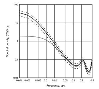
The autoregressive analysis of this time series showed an AR(5) model as optimal. Its spectral density estimates are shown in Fig. $6.8 \mathrm{~b}$. The low-frequency part of the spectrum up to $0.5$ cpy contains about $70 \%$ of the NINO3 variance and the ratio of the white noise RMS to the NINO3 RMS is 0.39. In contrast to the annual global

temperature with the trend present, the predictability of NINO3 diminishes quite fast, but, as seen from Fig. 6.9, it still extends to several months.

A KWT prediction from the end of 2017 through January 2019 is given in Fig. $6.10 \mathrm{a}$. The result of the test turned out to be satisfactory but one has to remember that the $90 \%$ confidence limits for the extrapolated values are rather wide. Only the first four or five predicted values lie within the relatively narrow interval not exceeding $\pm \sigma_{x}$

统计代写|时间序列分析代写Time-Series Analysis代考|Madden-Julian Oscillation

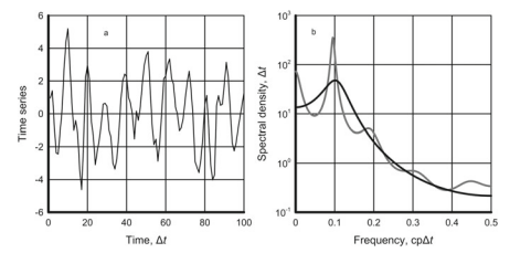
This data set is taken from site #7 in Appendix below. As mentioned in Chap. 5 , the components of MJO regarded as samples of scalar processes may possess relatively high statistical predictability. At the unit lead time (one day), the statistical predictability criterion $\rho$ (1) for the RMM1 component equals to about $0.18$ and the process should be studied in more detail. The predictability of the RMM1 time series decreases rather fast (Fig. 6.12), but it stays acceptable up to 6 days. The RMM2 component behaves in the same way.

Prediction examples (Fig. 6.13) turned out to be rather successful even for longer lead times, but the confidence bounds are rather wide. The cycles with periods close to 50 days cannot be reliably reproduced by the extrapolation trajectory at lead times close to the period of the cycle.

If the sampling rate is increased from 1 day to 10 days, the resulting time series becomes poorly predictable even at the unit lead time, that is, at 10 days. As both the original time series RMM1 and RMM2 and the time series with $\Delta t=10$ days are Gaussian or close to Gaussian, one can say that the Madden-Julian Oscillation is practically unpredictable at that sampling rate in spite of the presence of a significant spectral maximum.

The examples in this chapter include five rather typical and at the same time dissimilar cases with the sampling rates of one year, one month, and one day; they can be summed up in the following way:

the global surface temperature that has some predictability due to the dominant role of low-frequency variations even when the linear trend is deleted.
highly predictable Quasi-Biennial Oscillation whose spectrum contains a powerful peak at the low-frequency part of the spectrum,

SOI-the atmospheric component of ENSO-which contains a statistically significant spectral maximum and still has low predictability because of the low dynamic range of its spectrum.
MJO, with its smooth spectral maximum and acceptable forecasts at several lead times.

In conclusion, it has been shown here that the use of a forecasting method which agrees with the Kolmogorov-Wiener theory of extrapolation produces satisfactory results if the spectrum of the time series is concentrated within a relatively narrow frequency band. If the spectrum is spread more or less evenly over frequency, the time series is practically unpredictable. In all cases, even when the latest and previously unknown values of the time series lie close to the predicted trajectory, one should keep in mind the width of the confidence interval as a function of lead time. It is the quantity that defines the usefulness of forecasts.

时间序列分析代考

统计代写|时间序列分析代写Time-Series Analysis代考|Quasi-Biennial Oscillation

准双年振荡将在此处讨论Δ吨=1月。此示例使用的时间序列是问乙○在大气压水平20H磷一个，这对应于大约的高度26 ķ米高于平均海平面（图6.5一个和# 2# 2在附录中）。谱密度估计如图 1 所示。6.5 b频率轴以线性比例给出。

在撰写本文时，可获取 1953 年 1 月至 2019 年 4 月期间的 QBO 月度观察结果。2019 年 12 月添加的整个 2018 年和 2019 年接下来六个月（从 5 月到 11 月）的测试推断基于 12 月结束的时间序列部分2017(ñ=780).

根据此处使用的五个订单选择标准中的三个，最优的是订单的 AR 模型p=10 :

X吨=披1X吨−1+披2X吨−2+⋯+披10X吨−10+一个吨.
这意味着外推方程是

X^吨(τ)=披1X^吨(τ−1)+披2X^吨(τ−2)+⋯+披10X^吨(τ−10)白噪声方差对应于和⁡(10)模型是σ一个2≈21( 米/s)2而风速的总方差为20H磷一个是σX2≈389( 米/s)2. 因此，可预测性准则ρ(1)≈0.05和相关系数(6.13)在提前期风速的未知真实值和预测值之间τ=1月份是0.97. 从图 6.6 可以看出，问乙○在20H磷一个用可预测性标准描述的水平r和(τ)和ρ(τ)相当高。

初始时间在 2017 年 12 月的预测检验结果（图 6.7a）表明，外推的 AR 方法在这个时间序列上运行良好：20 个月度预测中有 19 个保持在90%置信限度。从 2018 年 12 月到 2021 年 1 月给出了更多预测，以供未来验证（图 6.7b）。用于 AR 模型的数据分别为 1953 年 1 月至 2017 年 12 月和 2018 年 12 月。当这本书准备好供出版商使用时，更多的观察结果变得可用，它们被包含在图 6.7b 中。外推的质量似乎很高，但应该记住，90%图中显示的置信区间很宽。

统计代写|时间序列分析代写Time-Series Analysis代考|ENSO Components

预测海洋ENSO 分量的行为——赤道太平洋的海表温度——被认为是气候学和海洋学中一项非常重要的任务（例如，附录中的#3 和#4）。预测ENSO 的大气成分——南方涛动指数——的尝试似乎并不多（例如，Kepenne 和Ghil 1992）。在本节中，这两个任务都将在 KWT 框架内处理。

在年采样率下，ENSO 分量的行为类似于白噪声（第 5 章）；他们通过任何概率方法进行的预测实际上都是无用的。在本例中，ENSO 地区 NINO3 的海面温度统计预报(5∘ñ−5∘小号,150∘在−90∘在)和南方涛动指数分别使用 1854 年 1 月至 2019 年 2 月和 1876 年至 2019 年 2 月的数据以每月采样率执行。数据可在以下附录中给出的网站#5 和#6 上获得。NINO3 时间序列如图 6.8a 所示。它可以被视为一个平稳过程的样本。
该时间序列的自回归分析表明 AR(5) 模型是最优的。其谱密度估计如图 1 所示。6.8 b. 频谱的低频部分高达0.5cpy 包含大约70%NINO3 方差和白噪声 RMS 与 NINO3 RMS 之比为 0.39。与每年的全球

随着温度的变化趋势，NINO3 的可预测性下降得相当快，但从图 6.9 可以看出，它仍然延续到几个月。

从 2017 年底到 2019 年 1 月的 KWT 预测如图 1 所示。6.10一个. 测试结果证明是令人满意的，但人们必须记住，90%外推值的置信限相当宽。只有前四个或五个预测值位于相对狭窄的区间内，不超过±σX

统计代写|时间序列分析代写Time-Series Analysis代考|Madden-Julian Oscillation

该数据集取自以下附录中的站点 #7。如第 1 章所述。如图5所示，作为标量过程样本的MJO的分量可能具有较高的统计可预测性。在单位提前期（一天），统计可预测性标准ρ(1) 对于 RMM1 组件，大约等于0.18并且应该更详细地研究这个过程。RMM1 时间序列的可预测性下降得相当快（图 6.12），但在 6 天之内仍然可以接受。RMM2 组件的行为方式相同。

预测示例（图 6.13）即使在较长的交付周期内也相当成功，但置信区间相当宽。周期接近 50 天的周期不能通过接近周期周期的提前期的外推轨迹可靠地再现。

如果采样率从 1 天增加到 10 天，即使在单位提前期（即 10 天）时，所得到的时间序列也变得难以预测。作为原始时间序列 RMM1 和 RMM2 以及具有Δ吨=10天是高斯或接近高斯，可以说，尽管存在显着的光谱最大值，但在该采样率下，马登-朱利安振荡实际上是不可预测的。

本章的例子包括五个比较典型但又不同的案例，采样率分别为一年、一个月和一天；它们可以用以下方式总结：

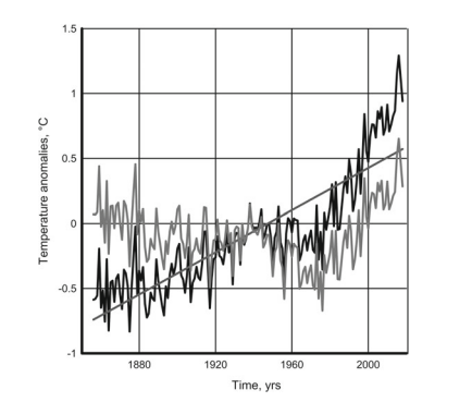
由于低频变化的主导作用，即使在线性趋势被删除的情况下，全球地表温度也具有一定的可预测性。
高度可预测的准两年振荡，其频谱在频谱的低频部分包含一个强大的峰值，

SOI——ENSO 的大气成分——包含一个统计上显着的光谱最大值，并且由于其光谱的低动态范围而仍然具有低的可预测性。
MJO，具有平滑的光谱最大值和在几个前置时间可接受的预测。

总之，这里已经表明，如果时间序列的频谱集中在相对窄的频带内，使用符合 Kolmogorov-Wiener 外推理论的预测方法会产生令人满意的结果。如果频谱在频率上或多或少地分布均匀，则时间序列实际上是不可预测的。在所有情况下，即使时间序列的最新值和以前未知的值接近预测轨迹，也应牢记置信区间的宽度与前置时间的函数关系。它是定义预测有用性的数量。

统计代写|时间序列分析代写Time-Series Analysis代考请认准statistics-lab™

统计代写请认准statistics-lab™. statistics-lab™为您的留学生涯保驾护航。

金融工程代写

金融工程是使用数学技术来解决金融问题。金融工程使用计算机科学、统计学、经济学和应用数学领域的工具和知识来解决当前的金融问题，以及设计新的和创新的金融产品。

非参数统计代写

非参数统计指的是一种统计方法，其中不假设数据来自于由少数参数决定的规定模型；这种模型的例子包括正态分布模型和线性回归模型。

广义线性模型代考

广义线性模型（GLM）归属统计学领域，是一种应用灵活的线性回归模型。该模型允许因变量的偏差分布有除了正态分布之外的其它分布。

术语广义线性模型（GLM）通常是指给定连续和/或分类预测因素的连续响应变量的常规线性回归模型。它包括多元线性回归，以及方差分析和方差分析（仅含固定效应）。

有限元方法代写

有限元方法（FEM）是一种流行的方法，用于数值解决工程和数学建模中出现的微分方程。典型的问题领域包括结构分析、传热、流体流动、质量运输和电磁势等传统领域。

有限元是一种通用的数值方法，用于解决两个或三个空间变量的偏微分方程（即一些边界值问题）。为了解决一个问题，有限元将一个大系统细分为更小、更简单的部分，称为有限元。这是通过在空间维度上的特定空间离散化来实现的，它是通过构建对象的网格来实现的：用于求解的数值域，它有有限数量的点。边界值问题的有限元方法表述最终导致一个代数方程组。该方法在域上对未知函数进行逼近。[1] 然后将模拟这些有限元的简单方程组合成一个更大的方程系统，以模拟整个问题。然后，有限元通过变化微积分使相关的误差函数最小化来逼近一个解决方案。

tatistics-lab作为专业的留学生服务机构，多年来已为美国、英国、加拿大、澳洲等留学热门地的学生提供专业的学术服务，包括但不限于Essay代写，Assignment代写，Dissertation代写，Report代写，小组作业代写，Proposal代写，Paper代写，Presentation代写，计算机作业代写，论文修改和润色，网课代做，exam代考等等。写作范围涵盖高中，本科，研究生等海外留学全阶段，辐射金融，经济学，会计学，审计学，管理学等全球99%专业科目。写作团队既有专业英语母语作者，也有海外名校硕博留学生，每位写作老师都拥有过硬的语言能力，专业的学科背景和学术写作经验。我们承诺100%原创，100%专业，100%准时，100%满意。

随机分析代写

随机微积分是数学的一个分支，对随机过程进行操作。它允许为随机过程的积分定义一个关于随机过程的一致的积分理论。这个领域是由日本数学家伊藤清在第二次世界大战期间创建并开始的。

时间序列分析代写

随机过程，是依赖于参数的一组随机变量的全体，参数通常是时间。随机变量是随机现象的数量表现，其时间序列是一组按照时间发生先后顺序进行排列的数据点序列。通常一组时间序列的时间间隔为一恒定值（如1秒，5分钟，12小时，7天，1年），因此时间序列可以作为离散时间数据进行分析处理。研究时间序列数据的意义在于现实中，往往需要研究某个事物其随时间发展变化的规律。这就需要通过研究该事物过去发展的历史记录，以得到其自身发展的规律。

回归分析代写

多元回归分析渐进（Multiple Regression Analysis Asymptotics）属于计量经济学领域，主要是一种数学上的统计分析方法，可以分析复杂情况下各影响因素的数学关系，在自然科学、社会和经济学等多个领域内应用广泛。

MATLAB代写

MATLAB 是一种用于技术计算的高性能语言。它将计算、可视化和编程集成在一个易于使用的环境中，其中问题和解决方案以熟悉的数学符号表示。典型用途包括：数学和计算算法开发建模、仿真和原型制作数据分析、探索和可视化科学和工程图形应用程序开发，包括图形用户界面构建MATLAB 是一个交互式系统，其基本数据元素是一个不需要维度的数组。这使您可以解决许多技术计算问题，尤其是那些具有矩阵和向量公式的问题，而只需用 C 或 Fortran 等标量非交互式语言编写程序所需的时间的一小部分。MATLAB 名称代表矩阵实验室。MATLAB 最初的编写目的是提供对由 LINPACK 和 EISPACK 项目开发的矩阵软件的轻松访问，这两个项目共同代表了矩阵计算软件的最新技术。MATLAB 经过多年的发展，得到了许多用户的投入。在大学环境中，它是数学、工程和科学入门和高级课程的标准教学工具。在工业领域，MATLAB 是高效研究、开发和分析的首选工具。MATLAB 具有一系列称为工具箱的特定于应用程序的解决方案。对于大多数 MATLAB 用户来说非常重要，工具箱允许您学习和应用专业技术。工具箱是 MATLAB 函数（M 文件）的综合集合，可扩展 MATLAB 环境以解决特定类别的问题。可用工具箱的领域包括信号处理、控制系统、神经网络、模糊逻辑、小波、仿真等。

R语言代写	问卷设计与分析代写
PYTHON代写	回归分析与线性模型代写
MATLAB代写	方差分析与试验设计代写
STATA代写	机器学习/统计学习代写
SPSS代写	计量经济学代写
EVIEWS代写	时间序列分析代写
EXCEL代写	深度学习代写
SQL代写	各种数据建模与可视化代写

统计代写|时间序列分析代写Time-Series Analysis代考|QBUS3850

Posted on 2022年6月9日2022年6月9日 by statistics-lab

如果你也在怎样代写时间序列分析Time-Series Analysis这个学科遇到相关的难题，请随时右上角联系我们的24/7代写客服。

我们提供的时间序列分析Time-Series Analysis及其相关学科的代写，服务范围广, 其中包括但不限于:

Statistical Inference 统计推断
Statistical Computing 统计计算
Advanced Probability Theory 高等概率论
Advanced Mathematical Statistics 高等数理统计学
(Generalized) Linear Models 广义线性模型
Statistical Machine Learning 统计机器学习
Longitudinal Data Analysis 纵向数据分析
Foundations of Data Science 数据科学基础

统计代写|时间序列分析代写Time-Series Analysis代考|QBUS3850

统计代写|时间序列分析代写Time-Series Analysis代考|General Remarks

Forecasting geophysical processes is probably the most desired goal in Earth and related solar sciences. Reliable predictions are needed at time scales from hours and days (meteorology, hydrology, etc.) to decades and centuries (climatology and related sciences). With one exception, all geophysical processes in the atmosphereocean-land-cryosphere system are random, which means that none of them can be predicted at any lead time without an error. The exception is tides-a deterministic process which exists in the oceans, atmosphere, and in the solid body of the planet. The knowledge of tides is especially important for the oceans, and tides in the open ocean can be predicted almost precisely. Along the shorelines where tides play an important role, sealevel variations can generally be predicted with sufficient accuracy as well, but there may be some cases when random disturbances should also be taken into account (Munk and Cartwright 1966).

The behavior of another astronomically caused process – the seasonal trend-is so irregular that one cannot even say for sure whether the next summer (or any other season) will be warmer or cooler than the current one.

The atmospheric, oceanic, terrestrial, and cryospheric processes and their interactions can be described with fluid dynamics equations; however, the equations are complicated, numerous, and cannot be solved analytically. Getting reliable numerical solutions encounters serious physical and computational problems, which cannot be discussed in this book. However, there is at least one important example of successful numerical solution of prediction problems – the weather forecasting. The forecasts given by meteorologists are reliable and rarely contain serious errors at lead times at least up to about a week. These forecasts are obtained by uploading information about the current (initial) state of processes involved in weather generation into a numerical computational scheme having discrete temporal and spatial resolution and then running the scheme forward in time and space to obtain forecasts. As the knowledge of the initial conditions cannot be ideal, the forecasts contain errors. Besides, the computational grid is discrete so that the processes whose scales are smaller than the distance between the grid nodes and shorter than the unit time step cannot be directly taken into account. The errors in the initial and other conditions grow with the forecast lead time, and eventually, the variance of the forecast errors becomes equal to the variance of the process that is being forecasted. The forecast becomes unusable. It means that the process has a predictability limit; the limit should be defined quantitatively through the ratio of the forecast error variance as a function of lead time to the variance of the process. These issues have been discussed in a number of classical works by Lorenz (1963, 1975, 1995).

统计代写|时间序列分析代写Time-Series Analysis代考|Method of Extrapolation

In both scalar and multivariate cases, the extrapolation means a forecast of the time series on the basis of its behavior in the past. The method of extrapolation used in this book to predict the behavior of stationary geophysical time series is based upon the autoregressive modeling (Box et al. 2015). It is discussed in this chapter for the case of scalar time series $x_{t}$ known over a finite time interval from $t=\Delta t$ through $t=N \Delta t$. The sampling interval $\Delta t$ is the unit time step, which can be a minute, hour, month, year, or whatever the data prescribes. Here, $\Delta t=1$. The only

assumption made about the time series $x_{t}$ is that it presents a sample record of a stationary random process.

The first stage of extrapolation procedure is to approximate the scalar time series with an AR model of a properly selected order $p$. The result of approximation is
$$
x_{t}=\varphi_{1} x_{t-1}+\cdots+\varphi_{p} x_{t-p}+a_{t},
$$
where $\varphi_{j}, j=1, \ldots, p$ are the AR coefficients and $a_{t}$ is a zero mean innovation sequence (white noise) with the variance $\sigma_{a}^{2}$.

Equation (6.1) describes the time series as a function of its behavior in the past, that is, exactly what is required for time series extrapolation. The unknown true value of the time series at lead time $\tau$ is
$$
x_{t+\tau}=\varphi_{1} x_{t+\tau-1}+\cdots+\varphi_{p} x_{t+\tau-p}+a_{t+\tau}
$$
so that at the lead time $\tau=1$
$$
x_{t+1}=\varphi_{1} x_{t}+\cdots+\varphi_{p} x_{t-p+1}+a_{t+1}
$$
At time $t$, all terms in the right-hand side of this equation, with the exception of $a_{t+1}$, are known because they belong to the observed initial time series. Therefore, the extrapolated (predicted, forecasted) value of the time series at the unit lead time is
$$
\hat{x}{t}(1)=\varphi{1} x_{t}+\cdots+\varphi_{p} x_{t-p+1} .
$$
As the extrapolation error at the unit lead time is $a_{t+1}$, its variance is $\sigma_{a}^{2}$. For $\tau=2$, one has
$$
\hat{x}{t}(2)=\varphi{1} \hat{x}{t}(1)+\cdots+\varphi{p} x_{t-p+2}
$$
so that the extrapolation error will be the sum of $\sigma_{a}^{2}$ with the error at $\tau=1$ (that is, $\sigma_{a}^{2}$ ) multiplied by the autoregression coefficient $\varphi_{1}$. The general solution for the extrapolation of an $\operatorname{AR}(p)$ sequence at the lead time $\tau$ is
$$
\hat{x}{t}(\tau)=\varphi{1} \hat{x}{t}(\tau-1)+\cdots+\varphi{p} \hat{x}_{t}(\tau-p)
$$

统计代写|时间序列分析代写Time-Series Analysis代考|Global Annual Temperature

According to Table 5.2, the higher predictability occurs for the annual surface temperature averaged over very large areas, up to the entire surface of the planet. This happens because respective time series contain most of their energy within the low-frequency part of the spectrum.

The global annual temperature (notated here as GLOBE) from 1850 (#1 in Appendix below and Fig. 6.1a) shows two intervals with a definite positive trend; the trend is longer and slightly faster during the latest several decades. Similar to the earlier interval from 1911 through 1944 , the trend that happened during the years from 1974 through 2010 (the initial year for our extrapolation test below) may have been caused by natural factors (Privalsky and Fortus 2011) so that its higher predictability could have been the result of regular variations of climate. As for the higher frequencies, the spectral density estimate for the detrended time series (Fig. 6.1b) proves

that detrending the time series does not affect the spectrum at frequencies above $0.02$ cpy (at time scales 50 years and shorter).

The goal of this test is to get an idea of extrapolation efficiency for the original and detrended time series. With year 2010 as the initial time for extrapolation, one has eight observed values of temperature anomalies that can be compared with predictions for 2011-2018.

The entire time series of GLOBE from 1850 through 2018 can be regarded as a sample of a stationary random process and extrapolated in accordance with its best fitting AR model. The second approach regards the time series as nonstationary: the sum of a stationary process plus trend (linear, in our case). The first version means that the trend is a part of the low-frequency variations caused by the natural climate variability; in the second version, the climate variability is regarded as stationary while the trend is caused by some external factors, including possible anthropogenic effects.

时间序列分析代考

统计代写|时间序列分析代写Time-Series Analysis代考|General Remarks

预测地球物理过程可能是地球和相关太阳科学中最理想的目标。从几小时和几天（气象学、水文等）到几十年和几个世纪（气候学和相关科学）的时间尺度上都需要可靠的预测。除了一个例外，大气-海洋-陆地-冰冻圈系统中的所有地球物理过程都是随机的，这意味着在任何提前期都无法无误地预测它们。潮汐是一个例外——一种存在于海洋、大气和地球固体中的确定性过程。潮汐知识对海洋尤为重要，几乎可以准确预测开阔海域的潮汐。沿着潮汐发挥重要作用的海岸线，通常也可以以足够的准确度预测海平面变化，

另一个由天文引起的过程——季节性趋势——的行为是如此不规则，以至于人们甚至无法确定下一个夏天（或任何其他季节）是否会比当前的夏天更温暖或更凉爽。

大气、海洋、陆地和冰冻圈过程及其相互作用可以用流体动力学方程来描述；然而，方程复杂、数量众多，无法解析求解。获得可靠的数值解会遇到严重的物理和计算问题，这本书无法讨论。然而，至少有一个成功的预测问题数值解的重要例子——天气预报。气象学家给出的预测是可靠的，并且在至少一周左右的提前期很少出现严重错误。这些预报是通过将有关天气生成过程的当前（初始）状态的信息上传到具有离散时间和空间分辨率的数值计算方案中获得的，然后在时间和空间上向前运行该方案以获得预报。由于初始条件的知识不可能是理想的，因此预测包含错误。此外，计算网格是离散的，因此不能直接考虑尺度小于网格节点之间距离且小于单位时间步长的过程。初始条件和其他条件下的误差随着预测提前期而增长，最终，预测误差的方差等于被预测过程的方差。预测变得不可用。这意味着该过程具有可预测性限制；限制应通过作为前置时间函数的预测误差方差与过程方差的比率来定量定义。Lorenz (1963, 1975, 1995) 的许多经典著作都讨论了这些问题。

统计代写|时间序列分析代写Time-Series Analysis代考|Method of Extrapolation

在标量和多变量情况下，外推意味着根据过去的行为对时间序列进行预测。本书中用于预测静止地球物理时间序列行为的外推方法基于自回归模型（Box et al. 2015）。本章讨论标量时间序列的情况X吨在有限的时间间隔内已知吨=Δ吨通过吨=ñΔ吨. 采样间隔Δ吨是单位时间步长，可以是一分钟、一小时、一个月、一年或任何数据规定的时间。这里，Δ吨=1. 唯一的

关于时间序列的假设X吨是它呈现了一个平稳随机过程的样本记录。

外推程序的第一阶段是用正确选择阶数的 AR 模型来近似标量时间序列p. 近似的结果是

X吨=披1X吨−1+⋯+披pX吨−p+一个吨,
在哪里披j,j=1,…,p是 AR 系数和一个吨是具有方差的零均值创新序列（白噪声）σ一个2.

等式 (6.1) 将时间序列描述为其过去行为的函数，也就是说，正是时间序列外推所需要的。提前期时间序列的未知真实值τ是

X吨+τ=披1X吨+τ−1+⋯+披pX吨+τ−p+一个吨+τ
所以在交货时间τ=1

X吨+1=披1X吨+⋯+披pX吨−p+1+一个吨+1
当时吨, 这个等式右边的所有项，除了一个吨+1, 是已知的，因为它们属于观察到的初始时间序列。因此，时间序列在单位提前期的外推（预测、预测）值为

X^吨(1)=披1X吨+⋯+披pX吨−p+1.
由于单位提前期的外推误差为一个吨+1，其方差为σ一个2. 为了τ=2, 一个有

X^吨(2)=披1X^吨(1)+⋯+披pX吨−p+2
因此外推误差将是σ一个2错误在τ=1（那是，σ一个2) 乘以自回归系数披1. 外推的一般解决方案和⁡(p)提前期的顺序τ是

X^吨(τ)=披1X^吨(τ−1)+⋯+披pX^吨(τ−p)

统计代写|时间序列分析代写Time-Series Analysis代考|Global Annual Temperature

根据表 5.2，在非常大的区域（直至地球的整个表面）的平均年表面温度具有较高的可预测性。发生这种情况是因为各个时间序列的大部分能量都包含在频谱的低频部分。

1850 年以来的全球年温度（此处记为 GLOBE）（下面附录中的#1 和图 6.1a）显示了两个具有明确正趋势的区间；在最近的几十年中，这一趋势更长，速度略快。与 1911 年到 1944 年的早期区间类似，1974 年到 2010 年（我们下面外推测试的第一年）发生的趋势可能是由自然因素引起的（Privalsky 和 Fortus 2011），因此其较高的可预测性可以是气候规律变化的结果。至于更高的频率，去趋势时间序列的谱密度估计（图 6.1b）证明

去趋势时间序列不会影响以上频率的频谱0.02cpy（时间尺度为 50 年或更短）。

该测试的目的是了解原始时间序列和去趋势时间序列的外推效率。以 2010 年作为外推的初始时间，有 8 个观察到的温度异常值可以与 2011-2018 年的预测值进行比较。

GLOBE 从 1850 年到 2018 年的整个时间序列可以看作是一个平稳随机过程的样本，并根据其最佳拟合 AR 模型进行外推。第二种方法将时间序列视为非平稳的：平稳过程加上趋势的总和（在我们的例子中是线性的）。第一个版本意味着趋势是自然气候变率引起的低频变化的一部分；在第二个版本中，气候变率被认为是静止的，而趋势是由一些外部因素引起的，包括可能的人为影响。

统计代写请认准statistics-lab™. statistics-lab™为您的留学生涯保驾护航。

金融工程代写

非参数统计代写

非参数统计指的是一种统计方法，其中不假设数据来自于由少数参数决定的规定模型；这种模型的例子包括正态分布模型和线性回归模型。

广义线性模型代考

广义线性模型（GLM）归属统计学领域，是一种应用灵活的线性回归模型。该模型允许因变量的偏差分布有除了正态分布之外的其它分布。

有限元方法代写

随机分析代写

时间序列分析代写

回归分析代写

MATLAB代写

R语言代写	问卷设计与分析代写
PYTHON代写	回归分析与线性模型代写
MATLAB代写	方差分析与试验设计代写
STATA代写	机器学习/统计学习代写
SPSS代写	计量经济学代写
EVIEWS代写	时间序列分析代写
EXCEL代写	深度学习代写
SQL代写	各种数据建模与可视化代写

统计代写|时间序列分析代写Time-Series Analysis代考|Math5845

Posted on 2022年6月9日2022年6月9日 by statistics-lab

如果你也在怎样代写时间序列分析Time-Series Analysis这个学科遇到相关的难题，请随时右上角联系我们的24/7代写客服。

我们提供的时间序列分析Time-Series Analysis及其相关学科的代写，服务范围广, 其中包括但不限于:

Statistical Inference 统计推断
Statistical Computing 统计计算
Advanced Probability Theory 高等概率论
Advanced Mathematical Statistics 高等数理统计学
(Generalized) Linear Models 广义线性模型
Statistical Machine Learning 统计机器学习
Longitudinal Data Analysis 纵向数据分析
Foundations of Data Science 数据科学基础

统计代写|时间序列分析代写Time-Series Analysis代考|Math5845

统计代写|时间序列分析代写Time-Series Analysis代考|Properties of Time Series of Spatially Averaged Surface Temperature

With the exception of ENSO-related phenomena, the results of analysis of geophysical time series listed in Table $5.1$ do not contradict the hypothesis of the Markovian behavior of climate (Hasselmann 1976). Out of the 13 time series in Table 5.1, seven have orders not higher than 1 , which can be regarded as a confirmation of the hypothesis. The other six samples have low predictability, which does not differ much from predictability of the remaining seven time series. The predictability of AMO is better than in all other cases, and it may be high enough for practical applications. The AMO time series differs from other time series in the table in the sense that it is obtained by averaging SST over a large area of the North Atlantic; therefore, one can assume that the comparatively high rate of spectral density decrease and the higher predictability criterion $r_{e}(1) \approx 0.62$ for AMO could be the result of that averaging.

The global climate is better characterized with data obtained by averaging over large parts of the globe. The AMO time series is just a specific example of such averaging, but we have nine time series that show the surface temperature over the entire globe, its hemispheres, and oceanic and terrestrial parts. Those time series have been analyzed in Privalsky and Yushkov (2018) and found to have a more complicated structure and a higher predictability than the other time series studied in that work.

The data used in the above publication include the complete time series given by the University of East Anglia; most of the time series begin in 1850. The authors of the data files show that the degree of coverage during the XIX Century was poor. Following the example given in Dobrovolski (2000), we will study the same time series starting from 1920 , when the coverage with observations generally increases to $50 \%$ and higher for the global, hemispheric and oceanic data.

The results given in Table $5.2$ confirm one of the previous conclusions: the annual surface temperature averaged over large parts of the globe is best described with relatively complicated models having AR orders $p=3$ or $p=4$ and a relatively high statistical predictability. The results for the southern hemisphere as a whole and for its land follow a Markov model and have lower statistical predictability; they agree with our results obtained from the data given by the Goddard Institute of Space Studies (GISS). According to the GISS data for the southern hemisphere (#14 in Appendix), the autoregressive order $p=1$ and the criterion $r_{e}(1) \approx 0.55$.

The data sets show that spatial averaging on the global scale and over the northern hemisphere including its oceans and land produces time series whose properties differ quite significantly from what is shown in Table $5.1$ for individual climate indices. The optimal AR orders increase up to four, and the predictability criterion grows up to $0.82$ for the north hemispheric ocean. The reason for the behavior of temperature over the southern hemisphere for the time series which begin in 1920 is not clear, but it may be related to the change is statistical properties of the trivariate system consisting of the time series of global, land, and terrestrial time series. For example, the predictability criterion $r_{e}$ (1) for the entire time series is $0.74$ (Privalsky and Yushkov 2018 ) and $0.44$ for the time series that begins in 1920 . A more detailed description of the change is given in Chap. 14 .

统计代写|时间序列分析代写Time-Series Analysis代考|Quasi-Biennial Oscillation

The “rule of no significant sharp peaks” in climate spectra has at least one exception which is supported with decades of direct observations. At least one atmospheric process-the Quasi-Biennial Oscillation, or QBO-does not follow this rule. The QBO phenomenon exists in the equatorial stratosphere at altitudes from about 16 $\mathrm{km}$ to $50 \mathrm{~km}$, and it is characterized with quasi-periodic variations of the westerly and easterly wind speed. The period of oscillations is about 28 months, which corresponds to the frequency of about $0.43$ cpy. It has been discovered in the 1950 ‘s and investigated in a number of publications, in particular, in Holton and Lindzen (1972) who proposed a physical model for QBO. In the review of QBO research by Baldwin et al (2001), QBO is called “a fascinating example of a coherent, oscillating mean flow that is driven with propagating waves with periods unrelated to the resulting oscillation.” Some effects of QBO upon climate are discussed by Anstey and Shepherd $(2014)$.

The statistical properties of QBO such as its spectra and statistical predictability do not seem to have been analyzed within the framework of theory of random processes; this section (along with Chaps. 6 and 10) is supposed to fill this gap in the part related to $\mathrm{QBO}$ as a scalar and bivariate (Chap. 10) phenomenon. It will be analyzed here using the set of monthly observational data provided by the Institute of Meteorology of the Free University of Berlin for the time interval from 1953 through December 2018 (see #15 in Appendix and Naujokat 1986). The set includes monthly wind speed data in the equatorial stratosphere at seven atmospheric pressure levels, from 10 to $70 \mathrm{hPa}$; these levels correspond to altitudes from $31 \mathrm{~km}$ to $18 \mathrm{~km}$.

If the goal of the study were to analyze $\mathrm{QBO}$ as a scalar random process, the data could have been taken at the sampling interval $\Delta t=6$ months or even 1 year. As QBO’s statistical predictability at a monthly sampling rate will also be studied in Chap. 6, the sampling interval $\Delta t=1$ month is taken in this section as well. Examples of $\mathrm{QBO}$ variations are shown in Fig. 5.3.

The basic statistical characteristics of $\mathrm{QBO}$ are shown in Table 5.3. The average wind speed is easterly (negative), and it decreases below the $20 \mathrm{hPa}$ level turning eastward at the lowest level. The variance increases from the $10 \mathrm{hPa}$ level by about $10 \%$ to $15 \mathrm{hPa}$ and $20 \mathrm{hPa}$ and then gradually decreases downward by an order of magnitude. These facts are well known (e.g., Baldwin et al. 2001). The optimal AR models have orders from $p=11$ to $p=29$; such orders are too high for individual time domain analysis.

The typical shape of the spectrum shows an almost periodic random function of time at $f \approx 0.43$ cpy (Fig. 5.4a). The maximum is very narrow and completely dominates the spectrum so that a more detailed picture can only be seen when the scale is logarithmic along both axes (Fig. 5.4b). This seems to be an absolutely unique phenomenon at climatic time scales. At higher frequencies, the spectral density diminishes rather quickly with all other peaks being statistically insignificant. Having this in mind, the spectra will be shown in what follows at frequencies not exceeding 1 cpy.

统计代写|时间序列分析代写Time-Series Analysis代考|Other Oscillations

The Madden-Julian Oscillation (MJO) is another unusual phenomenon both because it is not firmly fixed geographically and because it presents an oscillatory system not related to tides or to a seasonal trend. A review of MJO can be found in Zhang (2005).
Strictly speaking, the MJO phenomenon is a vector process and its spectra should be estimated in agreement with the approach discussed in Thomson and Emery (2014, Chap. 5). However, having in mind the methodological goals of the book, the MJO components will be treated here as either two scalar time series (this chapter and Chap. 6) or as a bivariate process (Chap. 8).

The MJO data used here consist of daily MJO indices RMM1 and RMM2 from January 1, 1979 through April 30, $2017(N=14000, \Delta t=1$ day). Thus, MJO is a bivariate random process. The source of the data is the Australian Bureau of Meteorology, site #16 in Appendix. The graph of the time series is shown in Fig. 5.6a. The hypothesis of stationarity can be accepted through visual assessment, but it is also confirmed by using the method described in Chap. 4. The spectral densities of the time series components are very similar and contain a single wide peak at the frequency close to $0.02 \mathrm{cpd}$. The spectral estimates are shown in Fig. $5.6 \mathrm{~b}$ for the part of the frequency axis up to $0.05 \mathrm{cpd}$; at higher frequencies, the spectrum is monotonically decreasing. The confidence limits are not shown because they almost coincide with the spectra due to the high reliability of estimates obtained with these long time series. The contribution of higher frequencies is negligibly small. Thus, the Madden-Julian Oscillation presents a good example of an oscillatory system. The statistical predictability criterion $r_{e}(1)$ given with Eq. (3.7) amounts to about $0.98$, meaning that both components possess high statistical predictability at the unit lead time, that is, at 1 day.

时间序列分析代考

统计代写|时间序列分析代写Time-Series Analysis代考|Properties of Time Series of Spatially Averaged Surface Temperature

除ENSO相关现象外，地球物理时间序列分析结果见表5.1不与马尔可夫气候行为的假设相矛盾（Hasselmann 1976）。在表 5.1 中的 13 个时间序列中，有 7 个的阶数不高于 1，可以认为是对假设的确认。其他 6 个样本的可预测性较低，与其余 7 个时间序列的可预测性差别不大。AMO 的可预测性优于所有其他情况，对于实际应用来说可能已经足够高了。AMO 时间序列与表中其他时间序列的不同之处在于它是通过对北大西洋大片区域的 SST 进行平均获得的；因此，可以假设相对较高的光谱密度下降率和较高的可预测性标准r和(1)≈0.62因为 AMO 可能是该平均的结果。

通过对全球大部分地区进行平均获得的数据可以更好地表征全球气候。AMO 时间序列只是这种平均的一个具体示例，但我们有九个时间序列来显示整个地球、其半球以及海洋和陆地部分的表面温度。这些时间序列已在 Privalsky 和 Yushkov（2018 年）中进行了分析，发现与该工作中研究的其他时间序列相比，它们具有更复杂的结构和更高的可预测性。

上述出版物中使用的数据包括东英吉利大学给出的完整时间序列；大部分时间序列始于 1850 年。数据文件的作者表明，19 世纪的覆盖程度很差。按照 Dobrovolski (2000) 中给出的示例，我们将从 1920 年开始研究相同的时间序列，此时观测的覆盖范围通常增加到50%全球、半球和海洋数据更高。

表中给出的结果5.2确认先前的结论之一：全球大部分地区的年平均表面温度最好用具有 AR 阶的相对复杂的模型来描述p=3或者p=4和相对较高的统计可预测性。整个南半球及其陆地的结果遵循马尔可夫模型，统计可预测性较低；他们同意我们从戈达德空间研究所 (GISS) 提供的数据中获得的结果。根据南半球的 GISS 数据（附录中的#14），自回归顺序p=1和标准r和(1)≈0.55.

数据集显示，全球尺度和北半球（包括其海洋和陆地）的空间平均产生时间序列，其性质与表中所示的有很大差异5.1个别气候指数。最优 AR 阶数增加到四个，可预测性标准增加到0.82对于北半球海洋。从 1920 年开始的时间序列南半球温度变化的原因尚不清楚，但可能与由全球、陆地和陆地时间序列组成的三元系统的统计特性的变化有关时间序列。例如，可预测性标准r和(1) 对于整个时间序列0.74（Privalsky 和 Yushkov 2018 年）和0.44对于从 1920 年开始的时间序列。更改的更详细描述在第 1 章中给出。14.

统计代写|时间序列分析代写Time-Series Analysis代考|Quasi-Biennial Oscillation

气候光谱中“没有显着尖峰的规则”至少有一个例外，它得到了数十年直接观测的支持。至少有一个大气过程——准双年振荡，或 QBO——不遵循这一规则。QBO 现象存在于海拔约 16 度的赤道平流层。ķ米至50 ķ米, 其特点是西风和东风的准周期性变化。振荡周期约为 28 个月，对应的频率约为0.43cp。它在 1950 年代被发现并在许多出版物中进行了研究，特别是在 Holton 和 Lindzen (1972) 中提出了 QBO 的物理模型。在 Baldwin 等人 (2001) 对 QBO 研究的评论中，QBO 被称为“一个由传播波驱动的连贯、振荡平均流的迷人例子，其周期与产生的振荡无关。” Anstey 和 Shepherd 讨论了 QBO 对气候的一些影响(2014).

QBO 的统计特性，如光谱和统计可预测性，似乎没有在随机过程理论的框架内进行分析；本节（连同第 6 章和第 10 章）应该填补与问乙○作为标量和双变量（第 10 章）现象。此处将使用柏林自由大学气象研究所提供的 1953 年至 2018 年 12 月期间的月度观测数据集进行分析（见附录中的 #15 和 Naujokat 1986）。该集合包括赤道平流层在七个大气压水平下的每月风速数据，从 10 到70H磷一个; 这些级别对应于从31 ķ米至18 ķ米.

如果研究的目标是分析问乙○作为标量随机过程，数据可以在采样间隔内获取Δ吨=6几个月甚至一年。由于 QBO 在每月采样率下的统计可预测性也将在第 1 章中进行研究。6、采样间隔Δ吨=1本节也采用月份。示例问乙○变化如图 5.3 所示。

基本统计特征问乙○如表 5.3 所示。平均风速为东风（负），低于20H磷一个水平在最低水平向东转。方差从10H磷一个大约水平10%至15H磷一个和20H磷一个然后逐渐向下减少一个数量级。这些事实是众所周知的（例如，Baldwin et al. 2001）。最优 AR 模型的订单来自p=11至p=29; 这样的阶数对于单独的时域分析来说太高了。

频谱的典型形状显示了一个几乎周期性的时间随机函数F≈0.43cpy（图 5.4a）。最大值非常窄并且完全支配光谱，因此只有当比例尺沿两个轴呈对数时才能看到更详细的图片（图 5.4b）。这似乎是气候时间尺度上绝对独特的现象。在较高的频率下，频谱密度下降得相当快，而所有其他峰值在统计上都是不显着的。考虑到这一点，频谱将以不超过 1 cpy 的频率显示如下。

统计代写|时间序列分析代写Time-Series Analysis代考|Other Oscillations

Madden-Julian 振荡 (MJO) 是另一个不寻常的现象，既因为它在地理上没有牢固固定，也因为它呈现出与潮汐或季节性趋势无关的振荡系统。可以在 Zhang (2005) 中找到对 MJO 的评论。
严格来说，MJO 现象是一个矢量过程，其光谱的估计应与 Thomson 和 Emery（2014 年，第 5 章）中讨论的方法一致。然而，考虑到本书的方法论目标，MJO 组件在这里将被视为两个标量时间序列（本章和第 6 章）或双变量过程（第 8 章）。

这里使用的 MJO 数据包括从 1979 年 1 月 1 日到 4 月 30 日的每日 MJO 指数 RMM1 和 RMM2，2017(ñ=14000,Δ吨=1天）。因此，MJO 是一个二元随机过程。数据来源是澳大利亚气象局，附录中的站点 #16。时间序列图如图 5.6a 所示。平稳性假设可以通过视觉评估来接受，但也可以通过使用第 1 章中描述的方法来确认。4. 时间序列分量的谱密度非常相似，并且在接近的频率处包含一个宽峰0.02Cpd. 频谱估计如图 1 所示。5.6 b对于频率轴的部分高达0.05Cpd; 在较高频率下，频谱单调递减。未显示置信限，因为它们几乎与光谱重合，因为这些长时间序列获得的估计具有高可靠性。较高频率的贡献小到可以忽略不计。因此，Madden-Julian 振荡是振荡系统的一个很好的例子。统计可预测性标准r和(1)用方程给出。(3.7) 约等于0.98，这意味着这两个组件在单位交货期（即 1 天）具有较高的统计可预测性。

统计代写请认准statistics-lab™. statistics-lab™为您的留学生涯保驾护航。

金融工程代写

非参数统计代写

非参数统计指的是一种统计方法，其中不假设数据来自于由少数参数决定的规定模型；这种模型的例子包括正态分布模型和线性回归模型。

广义线性模型代考

广义线性模型（GLM）归属统计学领域，是一种应用灵活的线性回归模型。该模型允许因变量的偏差分布有除了正态分布之外的其它分布。

有限元方法代写

随机分析代写

时间序列分析代写

回归分析代写

MATLAB代写

R语言代写	问卷设计与分析代写
PYTHON代写	回归分析与线性模型代写
MATLAB代写	方差分析与试验设计代写
STATA代写	机器学习/统计学习代写
SPSS代写	计量经济学代写
EVIEWS代写	时间序列分析代写
EXCEL代写	深度学习代写
SQL代写	各种数据建模与可视化代写

统计代写|时间序列分析代写Time-Series Analysis代考|STAT4102

Posted on 2022年6月9日2022年6月9日 by statistics-lab

如果你也在怎样代写时间序列分析Time-Series Analysis这个学科遇到相关的难题，请随时右上角联系我们的24/7代写客服。

我们提供的时间序列分析Time-Series Analysis及其相关学科的代写，服务范围广, 其中包括但不限于:

Statistical Inference 统计推断
Statistical Computing 统计计算
Advanced Probability Theory 高等概率论
Advanced Mathematical Statistics 高等数理统计学
(Generalized) Linear Models 广义线性模型
Statistical Machine Learning 统计机器学习
Longitudinal Data Analysis 纵向数据分析
Foundations of Data Science 数据科学基础

统计代写|时间序列分析代写Time-Series Analysis代考|STAT4102

统计代写|时间序列分析代写Time-Series Analysis代考|Frequency Resolution of Autoregressive Spectral Analysis

The AR (or MEM) spectral estimation provides an analytical formula for the estimated spectrum. It means that the spectral resolution in the formula is such that the value of spectral density can be calculated at any frequency. This is true, but the actual resolution is defined by the AR order: the number of extrema and inflection points in the spectral curve corresponding to an $\operatorname{AR}(p)$ model cannot be higher than $p$ (see Sect. 4.3). Therefore, a high resolution requires a high AR order, but a high-order model cannot be obtained with a short time series.

By definition, a linearly regular random process does not contain any strictly periodic components. This feature may cause some doubts about the ability of parametric time series analysis designed for regular processes to detect sharp peaks at frequencies which are close to each other, for example, when the data contain harmonic oscillations. Actually, the ability of autoregressive spectral analysis in this respect is very high under just one condition: getting accurate results requires having enough data for analysis. (Certainly, this requirement holds for all nonparametric method of spectral analysis such as Blackman and Tukey’s, MTM, Welch’s, etc.)

A unique case of harmonic oscillations with perfectly known frequencies within the Earth system is tides. The frequencies of tidal constituents are known precisely from astronomy; the amplitudes are determined from observations. The autoregressive analysis in the frequency domain provides a convenient tool for estimating frequencies of harmonic oscillations that are contained in time series of tidal phenomena. If the frequencies are determined correctly in sea level observations, one may hope that they will also be determined correctly in any other stationary data.
The example below is designed to verify how accurately the maximum entropy spectral analysis can determine the frequencies of tidal constituents by analyzing the time series of sea level at station 9414317 , Pier $221 / 2$, San Francisco, USA, using $10^{5}$ hourly sea level observations starting from January 28,2000 . The data source is $# 3$ in Appendix. A part of the record (about 50 days) is shown in Fig. 4.7. The tides obviously dominate the record.

统计代写|时间序列分析代写Time-Series Analysis代考|Example of AR Analysis in Time and Frequency Domains

Consider the entire process of time series analysis using as an example the annual values of Tripole Index (TPI) for the Interdecadal Pacific Oscillation (Henley et al. 2015). The time series shown in Fig. $4.9$ extends from 1854 through $2018(N=165)$; it is closely related to other El Niño-Southern Oscillation indices but differs from them in some respects. The data source is taken from the Web site #5 in Appendix to this chapter. The time series does not contain any statistically significant trend, and its behavior allows one to assume, without any further analysis, that it can be treated as a sample of a stationary random process. The test for Gaussianity showed that the probability density function of this time series can be regarded as normal.

The time series has been analyzed in the time domain by fitting to it $\mathrm{AR}(p)$ models of orders from $p=0$ through $p=16$ (one-tenth of the time series length). Three of the five order selection criteria used in this book have chosen the order $p=3$ :
$$
x_{t} \approx 0.46 x_{t-1}-0.29 x_{t-2}+0.15 x_{t-3}+a_{t}
$$
The RMS error of all estimated AR coefficients equals to approximately $0.08$ so that the coefficients are statistically significant at the confidence level $0.9$ used in this book.

The estimates of the mean value and standard deviation are $\bar{x} \approx-0.15$ and $\hat{\sigma}_{x} \approx 0.61$. The respective confidence intervals for the mean value and variance estimates obtained for the TPI time series expressed with model (4.11) are [ $-0.25$,

$-0.04]$ and $[0.55,0.68]$. These confidence intervals are determined in accordance with Eqs. (4.1) -(4.4) using estimates of the numbers of independent observations $\bar{N}=93$ and $\hat{N}=130$ obtained for the AR(3) model (4.11). These values are calculated through the correlation function estimate under the assumption that the correlation function $r(k)$ at lags $k=1,2,3$ coincides with the sample estimates while its further values behave in the maximum entropy mode. This correlation function obtained according to Eq. (4.5) diminishes very fast so that the numbers of independent observations $\bar{N}$ and $\hat{N}$ do not differ drastically from the total number of observations $N$.

The innovation sequence variance $\sigma_{a}^{2} \approx 0.31$ and the predictability (persistence) criterion $r_{e}(1)=\sqrt{1-\sigma_{a}^{2} / \sigma_{x}^{2}}$ equals $0.17$ meaning that the unpredictable innovation sequence $a_{t}$ plays a dominant role in the time series of Tripole Index. This time series is quite close to a white noise sequence, and the variance of its prediction errors will be high.

统计代写|时间序列分析代写Time-Series Analysis代考|Properties of Climate Indices

At climatic time scales, the basic statistical properties of a large number of geophysical time series-about 3000 -has been summarized in the fundamental work by Dobrovolski $(2000)$ dealing with stochastic models of scalar climatic data. The time series in that book include surface temperature, atmospheric pressure, precipitation, sea level, and some other geophysical variables observed at individual stations; the data set includes 195 time series of sea surface temperature averaged within $5^{\circ} \times 5^{\circ}$ squares. Most of those time series are best approximated with either a white noise or a Markov process (Dobrovolski 2000 , p. 135). The white noise model AR(0) can be justly regarded as a specific case of the $\mathrm{AR}(1)$ model. The prevalence of the $\mathrm{AR}(1)$ model for climatic time series obtained without large-scale spatial averaging has been noted recently in Privalsky and Yushkov (2018), but the results given in Dobrovolski $(2000)$ are based upon a much larger observation base.

In this section, we will complement the available information by studying first a number of geophysical time series that are often used as climate indicators or indices; their names usually contain the term “oscillation” or “index.” The list is given in Table 5.1, and the data sources are shown in the Appendix to this chapter. In all cases, the value of $\Delta t$ is one year. Along with the optimal AR orders $p$ for the time series, the table contains the values of statistical predictability criterion (3.7): $r_{e}(1)=\sqrt{1-\sigma_{a}^{2} / \sigma_{x}^{2}}$, where $\sigma_{x}^{2}$ and $\sigma_{a}^{2}$ are the time series variance and the variance of its innovation sequence.

The sources of data listed in the table are given in Appendix to this chapter: the numbers in the first column of the table coincide with the numbers in the Appendix.
Two characteristic features are common for the time series in Table 5.1: all of them can be regarded as Gaussian, and, with one exception, all of them have low statistical predictability. This means that they present sample records of random processes similar to a white noise; that is, their behavior in the time domain is very irregular, and, consequently, none of them contains oscillations as the term is understood in physics. The exception is the relatively high predictability of the Atlantic Multidecadal Oscillation. Thus, judging by the low optimal AR orders and the low predictability, one may say that though the optimal model for most of these time series is not AR(1) their behavior does not contradict the assumption of the Markov character of climate variability and that the value of the autoregressive coefficient is significantly smaller than one.

时间序列分析代考

统计代写|时间序列分析代写Time-Series Analysis代考|Frequency Resolution of Autoregressive Spectral Analysis

AR（或 MEM）谱估计为估计的谱提供了一个分析公式。这意味着公式中的光谱分辨率使得光谱密度的值可以在任何频率下计算。这是真的，但实际分辨率由 AR 阶定义：光谱曲线中极值和拐点的数量对应于和⁡(p)型号不能高于p（见第 4.3 节）。因此，高分辨率需要高AR阶数，而时间序列短却无法得到高阶模型。

根据定义，线性规则随机过程不包含任何严格的周期性分量。此功能可能会导致对为常规过程设计的参数时间序列分析检测彼此接近的频率处的尖峰的能力产生一些疑问，例如，当数据包含谐波振荡时。实际上，自回归光谱分析在这方面的能力非常高，仅在一个条件下：获得准确的结果需要有足够的数据进行分析。（当然，此要求适用于所有非参数光谱分析方法，例如 Blackman 和 Tukey’s、MTM、Welch’s 等）

地球系统内具有完全已知频率的谐波振荡的一个独特情况是潮汐。潮汐成分的频率可以从天文学中准确得知；幅度由观察确定。频域中的自回归分析为估计包含在潮汐现象时间序列中的谐波振荡频率提供了一种方便的工具。如果在海平面观测中正确确定了频率，人们可能希望在任何其他固定数据中也能正确确定频率。
下面的示例旨在通过分析码头 9414317 站的海平面时间序列来验证最大熵谱分析如何准确地确定潮汐成分的频率221/2，美国旧金山，使用105从 2000 年 1 月 28 日开始的每小时海平面观测。数据源是# 3# 3在附录中。部分记录（约 50 天）如图 4.7 所示。潮汐显然占主导地位。

统计代写|时间序列分析代写Time-Series Analysis代考|Example of AR Analysis in Time and Frequency Domains

以年代际太平洋涛动的三极子指数 (TPI) 的年度值为例，考虑时间序列分析的整个过程（Henley 等人，2015 年）。时间序列如图所示。4.9从 1854 年延伸到2018(ñ=165); 它与其他厄尔尼诺-南方涛动指数密切相关，但在某些方面有所不同。数据源取自本章附录中的网站#5。时间序列不包含任何统计上显着的趋势，并且它的行为允许人们在没有任何进一步分析的情况下假设它可以被视为平稳随机过程的样本。高斯性检验表明，该时间序列的概率密度函数可视为正态。

时间序列已通过拟合在时域中进行了分析一个R(p)订单型号来自p=0通过p=16（时间序列长度的十分之一）。本书中使用的五个订单选择标准中的三个选择了订单p=3 :

X吨≈0.46X吨−1−0.29X吨−2+0.15X吨−3+一个吨
所有估计的 AR 系数的 RMS 误差大约等于0.08使得系数在置信水平上具有统计显着性0.9本书中使用。

平均值和标准差的估计是X¯≈−0.15和σ^X≈0.61. 用模型 (4.11) 表示的 TPI 时间序列的平均值和方差估计值各自的置信区间为 [−0.25,

−0.04]和[0.55,0.68]. 这些置信区间是根据方程式确定的。(4.1) -(4.4) 使用独立观察次数的估计ñ¯=93和ñ^=130为 AR(3) 模型 (4.11) 获得。这些值是在相关函数的假设下通过相关函数估计计算得出的r(ķ)在滞后ķ=1,2,3与样本估计值一致，而其进一步的值表现为最大熵模式。该相关函数根据方程式获得。(4.5) 减少得非常快，因此独立观察的数量ñ¯和ñ^与观察总数没有太大差异ñ.

创新序列方差σ一个2≈0.31和可预测性（持久性）标准r和(1)=1−σ一个2/σX2等于0.17意味着不可预测的创新序列一个吨在三极子指数的时间序列中起主导作用。这个时间序列非常接近白噪声序列，其预测误差的方差会很大。

统计代写|时间序列分析代写Time-Series Analysis代考|Properties of Climate Indices

在气候时间尺度上，Dobrovolski 在基础工作中总结了大量地球物理时间序列（约 3000 个）的基本统计特性(2000)处理标量气候数据的随机模型。那本书中的时间序列包括地表温度、大气压力、降水、海平面和在各个站观测到的其他一些地球物理变量；该数据集包括 195 个时间序列的平均海表温度5∘×5∘正方形。大多数这些时间序列最好用白噪声或马尔可夫过程来近似（Dobrovolski 2000，第 135 页）。白噪声模型 AR(0) 可以公正地看作是一个R(1)模型。的流行一个R(1)最近在 Privalsky 和 Yushkov (2018) 中注意到了在没有大尺度空间平均的情况下获得的气候时间序列模型，但在 Dobrovolski 中给出的结果(2000)是基于更大的观察基础。

在本节中，我们将通过首先研究一些经常用作气候指标或指数的地球物理时间序列来补充现有信息；它们的名称通常包含术语“振荡”或“指数”。列表见表 5.1，数据来源见本章附录。在所有情况下，价值Δ吨是一年。连同最佳的 AR 订单p对于时间序列，该表包含统计可预测性标准 (3.7) 的值：r和(1)=1−σ一个2/σX2，在哪里σX2和σ一个2是时间序列方差及其创新序列的方差。

表中数据来源见本章附录：表中第一栏数字与附录数字一致。
表 5.1 中的时间序列有两个共同的特征：它们都可以被认为是高斯的，并且除了一个例外，它们都具有低的统计可预测性。这意味着它们呈现类似于白噪声的随机过程的样本记录；也就是说，它们在时域中的行为非常不规则，因此它们都不包含物理学中所理解的振荡。例外是大西洋多年代际涛动的相对较高的可预测性。因此，从低最优 AR 阶数和低可预测性来看，

统计代写请认准statistics-lab™. statistics-lab™为您的留学生涯保驾护航。

金融工程代写

非参数统计代写

非参数统计指的是一种统计方法，其中不假设数据来自于由少数参数决定的规定模型；这种模型的例子包括正态分布模型和线性回归模型。

广义线性模型代考

广义线性模型（GLM）归属统计学领域，是一种应用灵活的线性回归模型。该模型允许因变量的偏差分布有除了正态分布之外的其它分布。

有限元方法代写

随机分析代写

时间序列分析代写

回归分析代写

MATLAB代写

R语言代写	问卷设计与分析代写
PYTHON代写	回归分析与线性模型代写
MATLAB代写	方差分析与试验设计代写
STATA代写	机器学习/统计学习代写
SPSS代写	计量经济学代写
EVIEWS代写	时间序列分析代写
EXCEL代写	深度学习代写
SQL代写	各种数据建模与可视化代写

统计代写|时间序列分析代写Time-Series Analysis代考|STAT8002

Posted on 2022年6月9日2022年6月9日 by statistics-lab

如果你也在怎样代写时间序列分析Time-Series Analysis这个学科遇到相关的难题，请随时右上角联系我们的24/7代写客服。

我们提供的时间序列分析Time-Series Analysis及其相关学科的代写，服务范围广, 其中包括但不限于:

Statistical Inference 统计推断
Statistical Computing 统计计算
Advanced Probability Theory 高等概率论
Advanced Mathematical Statistics 高等数理统计学
(Generalized) Linear Models 广义线性模型
Statistical Machine Learning 统计机器学习
Longitudinal Data Analysis 纵向数据分析
Foundations of Data Science 数据科学基础

统计代写|时间序列分析代写Time-Series Analysis代考|STAT8002

统计代写|时间序列分析代写Time-Series Analysis代考|Practical Analysis of Time Series

Abstract After a preliminary processing, the time series should be tested for stationarity. The test may fail if the time series contains a trend or if its mean value, variance, or spectrum are found to be time-dependent. Deleting the trend can be justified if it is caused by external factors or if it interferes with the higher-frequency part of the spectral density of interest to the researcher. A test for stationarity is suggested through splitting the time series in halves and estimating the mean values, variances and, if possible, spectral densities of the entire time series and its halves. The confidence bounds for estimates of statistical moments depend upon the number of independent observations in the time series. These numbers depend upon the correlation structure of the time series, and they can be much smaller than the total number of terms in the time series. A linear filtering is generally not recommended. The autoregressive approach allows one to determine frequencies of even strictly periodic oscillations contained in the time series (tides) with exceptionally high accuracy providing that the time series is long. A detailed example of autoregressive analysis is given.
The two mandatory requirements in practical analysis of time series are

using the proper methods of analysis and
calculating confidence intervals for all estimated statistical characteristics.
This means, in particular, that the methods of time and frequency domain analysis should be mathematically suitable for the time series which is being analyzed. In this book, the fundamental approach to analysis is based upon autoregressive modeling, which has the ability to provide relatively reliable estimates of time series statistics even with short time series. Its other advantage is the explicit time domain model which is obtained at the initial stage of autoregressive analysis and which does not exist if a nonparametric approach is used. It will be shown later in this chapter (Sect. 4.5) that the autoregressive approach can be quite effective for estimating the spectral density of time series with a very complicated structure.

If the time series is short, its spectrum should not be estimated with nonparametric methods other than Thomson’s MTM. Moreover, all statistical estimates should be accompanied with respective reliability estimates. Any estimate of statistical characteristics is absolutely useless if it is not supplemented with confidence intervals or

some other quantitative indicator of its reliability in accordance with mathematical statistics. If confidence intervals or reliability estimates are available but not shown intentionally, their absence should be explained.

If the time series contains outliers, they should be handled before continuing the analysis. The next step is to build an autoregressive model of the time series, including respective spectral estimate, and to check for any unexpected features such as a significant low-frequency trend and/or unexplainable spectral peaks in the model selected by most order selection criteria. The latter problem is rare because normally the order selection criteria do not allow unreasonably high or low orders. The information obtained at that stage should be used to decide if any additional steps might be required.
The common problems of this type include

an incorrect sampling interval,
the presence of a linear or nonlinear trend in the time series,
the presence of strong high-frequency and/or quasi-periodic fluctuations in the AR model’ spectrum, which need to be explained.

The trend can be a product of natural low-frequency components or it can be caused by some artificial external forcing (such as an anthropogenic effect). The decision whether to delete the trend or analyze the time series as is should not be taken without a justification.

统计代写|时间序列分析代写Time-Series Analysis代考|Selecting the Sampling Interval

The sampling interval $\Delta t$ should be set in agreement with the task of the analysis. If it is the climate variability at time scales longer than $2.5-3$ years, the interval $\Delta t=1$ year is generally sufficient. The resulting highest frequency in the time series spectrum is the Nyquist frequency $f_{N}=1 / 2 \Delta t$, that is, $0.5$ cpy when $\Delta t=1$ year. The frequencies that can be analyzed reliably begin from approximately $0.30-$ $0.35$ cpy. Simple interpolation between consecutive terms of the time series intended to get a faster sampling rate is useless. If the spectrum is expected to contain high energy at higher frequencies, the interval should be smaller; such cases are rather rare in Earth sciences. Setting $\Delta t=1$ month for studying climate variability is normally not reasonable, in particular, because it may transform a stationary time series into a sample of a periodically correlated (cyclostationary) random process. Also, an exceedingly small sampling interval creates redundant information and reduces the spectral resolution at lower frequencies. The general rule here is that the time series should contain at least several measurements per the smallest time scale of interest. For example, the choice of $\Delta t=1$ year could be too large for studying the QuasiBiennial Oscillation whose characteristic time scale is approximately $2.3$ year. These considerations are relevant for other conditions when the time series is not related to climate and when time is measured in seconds, hours, or any other units.

统计代写|时间序列分析代写Time-Series Analysis代考|Testing for Stationarity and Ergodicity

The only assumption, which is made about time series for its standard statistical analysis, including spectral estimation, is that it belongs to a stationary random process. To prove with probability one that the assumption is correct is not possible but one can verify whether it can be acceptable for a specific time series. This may be done in the following manner:

split the time series in two equal parts and
verify that the differences between the statistics of the entire time series and its halves do not lie outside the limits of sampling variability of respective estimates for the entire time series.

If the results of such verification are favorable, that is, if the differences can be ascribed to the sampling variability, there seems to be no ground to reject the initial assumption of stationarity. If, in addition, the probability distribution of the time series is Gaussian, the hypothesis of ergodicity that is usually accepted for stationary time series by default becomes reasonable as well. Comparisons should include at least the first two statistical moments, that is, the mean value and variance (or the root mean square value). The variances of estimated mean values and estimated variances should be calculated with account for the number of statistically independent observations in the time series.

For the time series $x_{t}, t=1, \ldots, N$, the root mean square (RMS) error of the estimated mean value $\bar{x}$ is
$$
\sigma[\bar{x}] \approx \sigma_{x} / \sqrt{\bar{N}}
$$
where $\sigma_{x}$ is the estimated standard deviation and $\tilde{N}$ is the effective number of independent observations in the time series:
$$
\bar{N}=N / \sum_{k=-\infty}^{k=\infty} r(k)
$$
where $r(k)$ is the correlation function of the time series.
The RMS error of the estimated variance $\sigma_{x}^{2}$ is
$$
\sigma\left[\sigma_{x}^{2}\right]=\sigma_{x}^{2} / \hat{N}
$$
where
$$
\hat{N}=N / \sum_{k=-\infty}^{\infty} r^{2}(k)
$$

时间序列分析代考

统计代写|时间序列分析代写Time-Series Analysis代考|Practical Analysis of Time Series

摘要经过初步处理，时间序列应进行平稳性检验。如果时间序列包含趋势，或者如果发现其平均值、方差或频谱与时间相关，则测试可能会失败。如果趋势是由外部因素引起的，或者如果它干扰了研究人员感兴趣的频谱密度的高频部分，则删除趋势是合理的。建议通过将时间序列分成两半并估计平均值、方差以及（如果可能）整个时间序列及其两半的谱密度来进行平稳性检验。统计矩估计的置信界限取决于时间序列中独立观察的数量。这些数字取决于时间序列的相关结构，它们可以比时间序列中的项总数小得多。一般不推荐使用线性滤波。如果时间序列很长，自回归方法允许人们以异常高的精度确定时间序列（潮汐）中包含的甚至是严格的周期性振荡的频率。给出了自回归分析的详细示例。
时间序列实际分析中的两个强制性要求是

使用适当的分析方法和
计算所有估计统计特征的置信区间。
这尤其意味着时域和频域分析的方法在数学上应该适用于正在分析的时间序列。在本书中，分析的基本方法是基于自回归模型，它能够提供相对可靠的时间序列统计估计，即使是短时间序列。它的另一个优点是在自回归分析的初始阶段获得的显式时域模型，如果使用非参数方法则不存在。本章稍后（第 4.5 节）将表明，自回归方法对于估计具有非常复杂结构的时间序列的谱密度非常有效。

如果时间序列很短，则不应使用除 Thomson 的 MTM 之外的非参数方法估计其频谱。此外，所有统计估计都应附有各自的可靠性估计。任何统计特征的估计如果没有置信区间或

根据数理统计，其可靠性的其他一些量化指标。如果置信区间或可靠性估计可用但未有意显示，则应解释它们的缺失。

如果时间序列包含异常值，则应在继续分析之前对其进行处理。下一步是建立时间序列的自回归模型，包括各自的频谱估计，并检查任何意外特征，例如由大多数订单选择标准选择的模型中的显着低频趋势和/或无法解释的频谱峰值。后一个问题很少见，因为通常订单选择标准不允许不合理的高或低订单。应使用在该阶段获得的信息来决定是否需要采取任何额外的步骤。
这种类型的常见问题包括

不正确的采样间隔，
时间序列中存在线性或非线性趋势，
AR 模型频谱中存在强烈的高频和/或准周期性波动，这需要解释。

这种趋势可能是自然低频分量的产物，也可能是由一些人为的外部强迫（如人为影响）引起的。在没有正当理由的情况下，不应做出是否删除趋势或按原样分析时间序列的决定。

统计代写|时间序列分析代写Time-Series Analysis代考|Selecting the Sampling Interval

采样间隔Δ吨应与分析任务相一致。如果是时间尺度上的气候变率大于2.5−3年，间隔Δ吨=1一般一年就够了。时间序列频谱中产生的最高频率是奈奎斯特频率Fñ=1/2Δ吨，那是，0.5cpy什么时候Δ吨=1年。可以可靠分析的频率从大约0.30− 0.35cp。旨在获得更快采样率的时间序列的连续项之间的简单插值是没有用的。如果预期频谱在较高频率处包含高能量，则间隔应该更小；这种情况在地球科学中相当罕见。环境Δ吨=1研究气候变率的月份通常是不合理的，特别是因为它可能将平稳时间序列转换为周期性相关（循环平稳）随机过程的样本。此外，极小的采样间隔会产生冗余信息并降低较低频率的光谱分辨率。这里的一般规则是时间序列应该包含每个感兴趣的最小时间尺度至少几个测量值。例如，选择Δ吨=1年对于研究特征时间尺度约为的准双年振荡可能太大了2.3年。当时间序列与气候无关并且时间以秒、小时或任何其他单位测量时，这些考虑因素与其他条件相关。

统计代写|时间序列分析代写Time-Series Analysis代考|Testing for Stationarity and Ergodicity

对其标准统计分析（包括谱估计）的时间序列做出的唯一假设是它属于平稳随机过程。用概率证明假设是正确的是不可能的，但可以验证它对于特定的时间序列是否可以接受。这可以通过以下方式完成：

将时间序列分成两个相等的部分，并且
验证整个时间序列及其一半的统计数据之间的差异不超出整个时间序列各自估计值的抽样变异性限制。

如果这种验证的结果是有利的，也就是说，如果差异可以归因于抽样的可变性，那么似乎没有理由拒绝最初的平稳性假设。此外，如果时间序列的概率分布是高斯分布的，那么对于静止时间序列通常被默认接受的遍历性假设也变得合理。比较应至少包括前两个统计矩，即均值和方差（或均方根值）。估计平均值的方差和估计方差的计算应考虑时间序列中统计独立观察的数量。

对于时间序列X吨,吨=1,…,ñ, 估计平均值的均方根 (RMS) 误差X¯是

σ[X¯]≈σX/ñ¯
在哪里σX是估计的标准偏差和ñ~是时间序列中独立观察的有效数量：

ñ¯=ñ/∑ķ=−∞ķ=∞r(ķ)
在哪里r(ķ)是时间序列的相关函数。
估计方差的 RMS 误差σX2是

σ[σX2]=σX2/ñ^
在哪里

ñ^=ñ/∑ķ=−∞∞r2(ķ)

统计代写请认准statistics-lab™. statistics-lab™为您的留学生涯保驾护航。

金融工程代写

非参数统计代写

非参数统计指的是一种统计方法，其中不假设数据来自于由少数参数决定的规定模型；这种模型的例子包括正态分布模型和线性回归模型。

广义线性模型代考

广义线性模型（GLM）归属统计学领域，是一种应用灵活的线性回归模型。该模型允许因变量的偏差分布有除了正态分布之外的其它分布。

有限元方法代写

随机分析代写

时间序列分析代写

回归分析代写

MATLAB代写

R语言代写	问卷设计与分析代写
PYTHON代写	回归分析与线性模型代写
MATLAB代写	方差分析与试验设计代写
STATA代写	机器学习/统计学习代写
SPSS代写	计量经济学代写
EVIEWS代写	时间序列分析代写
EXCEL代写	深度学习代写
SQL代写	各种数据建模与可视化代写

统计代写|时间序列分析代写Time-Series Analysis代考|STATS 7058

Posted on 2022年6月9日2022年6月9日 by statistics-lab

如果你也在怎样代写时间序列分析Time-Series Analysis这个学科遇到相关的难题，请随时右上角联系我们的24/7代写客服。

我们提供的时间序列分析Time-Series Analysis及其相关学科的代写，服务范围广, 其中包括但不限于:

Statistical Inference 统计推断
Statistical Computing 统计计算
Advanced Probability Theory 高等概率论
Advanced Mathematical Statistics 高等数理统计学
(Generalized) Linear Models 广义线性模型
Statistical Machine Learning 统计机器学习
Longitudinal Data Analysis 纵向数据分析
Foundations of Data Science 数据科学基础

统计代写|时间序列分析代写Time-Series Analysis代考|STATS 7058

统计代写|时间序列分析代写Time-Series Analysis代考|Determining the Order of Autoregressive Models

Seemingly, the availability of an exact formula for the spectral density means that the frequency resolution of autoregressive and other parametric spectral estimates is infinitely high because it can be calculated at any frequency. However, as follows from Eq. (3.13), the number of peaks, troughs, and inflection points in autoregressive spectral density estimates cannot exceed the model’s order $p$. Therefore, the AR order is the key parameter that defines the features of an $\mathrm{AR}$ (or MEM) spectral estimate. Similar considerations are true for the moving average and mixed ARMA models.

The role of the order $p$ is convenient to characterize with the following simple example. Let $x_{t}, t=1, \ldots 100$, be a sample record of a dimensionless white noise process with a unit variance and the sampling interval $\Delta t$ (e.g., 1 year, 1 day, etc.). According to Eq. (3.13), the true spectrum is a constant: $s(f)=2 \sigma_{a}^{2} \Delta t$. As the true model of the time series is not known at the initial stage of analysis, the spectral estimates should be sought for several values of $p$, say, from $p=0$ through $p=10$ for a time series of length $N=100$. To select higher values of the AR order would be unreasonable because of common sense considerations: it is not possible to obtain reliable estimates if the number of quantities to be estimated is comparable to the number of observations. The results of analysis of the white noise sequence are shown in Fig. 3.1. Obviously, if one were to choose the AR order $p=10$ arbitrarily, the conclusion would be that the time series contains “cycles” or quasi-periodic components at frequencies about $0.11$ cycles per $\Delta t(\mathrm{cp} \Delta t$ ) and $0.39 \mathrm{cp} \Delta t$. However, the correctly defined confidence limits for the estimates given in Fig. $3.1$ show that such conclusions would have been false because one can draw a very smooth or even a horizontal line within the confidence interval for the estimate. Obviously, a high order (e.g., $p \geq 10$ ) does not necessarily mean that the spectral density contains significant peaks. An AR model having a high order may have a very smooth spectrum, while a low-order model can have very sharp peaks (see Fig. $2.8$ and the well-known AR(4) example given in the Percival and Walden book published in 1993, pp. 46, 148). Similar examples can be given for more complicated spectra, but the major conclusion is that determining the order of parametric models and showing a confidence interval constitute the absolutely necessary element of parametric spectral analysis.

统计代写|时间序列分析代写Time-Series Analysis代考|Comparison of Autoregressive and Nonparametric Spectral Estimates

The statement that the spectral density is the most important statistics of any scalar time series is true for Gaussian and non-Gaussian data. The spectral density can be estimated with parametric and nonparametric methods, and if the time series is long, the estimates will be reliable and similar to each other. If the time series is short, which happens regularly in climatology and its branches and in other Earth sciences, the task of proper spectral analysis becomes vital. In this section, we will show the advantages of the parametric approach to the task of spectral estimation, which exist, in particular, due to the fact that many geophysical processes can be well approximated with stochastic difference equations of relatively low order. The examples given here include time series whose spectra are typical for climatic processes, including the

annual global surface temperature. The time series will always be short: the total number of its terms is just 50 . The autoregressive spectral estimates will be compared with respective nonparametric estimates obtained according to Blackman and Tukey (1958). Four time series of length $N=50$ have AR orders from 1 to 4 , and they are quite common for climate and for other geophysical phenomena. The true AR models are known in all cases, and the initial data for the analysis were obtained through simulation. Because of the small length of the time series, the sample estimates of AR coefficients may differ rather significantly from the true values.

The true model of the first time series is an AR(1) with the AR coefficient $\varphi=0.5$. It can be the annual river streamflow, daily temperature, sea level variations in coastal areas with no tides, etc. The sample AR (or MEM) estimate of the spectrum is shown in Fig. 3.3a along with the true spectrum.

According to Fig. 3.3a, the $90 \%$ confidence interval for the AR spectral estimate contains the true spectrum; this estimate can be regarded as satisfactory. The shape of the spectrum is reproduced accurately, and the bias occurs due to the sampling variability of the variance estimate. The nonparametric estimate (Fig. 3.3b) has several peaks, but the peaks are statistically insignificant. The $90 \%$ confidence interval is wide and asymmetric with respect to the spectral estimate due to the asymmetry of $\chi^{2}$ distribution at low degrees of freedom in this and the other three examples below.

统计代写|时间序列分析代写Time-Series Analysis代考|Advantages and Disadvantages of Autoregressive Analysis

The autoregressive approach provides quantitative information about statistical properties of time series in both time and frequency domains. This can also be achieved with other parametric models, but the moving average operator is less reasonable physically and is difficult to deal with. The nonparametric methods of analysis do not produce explicit information about the time series behavior in the time domain and, if the time series is short, the nonparametric spectral estimates are less reliable than the AR estimates.

The autoregressive stochastic difference equation possesses a number of useful features for analysis of stationary time series:

it presents a ready-to-use tool for linear extrapolation of time series (Chap. 6);
it allows one to get quantitative estimates of time series dependence upon its previous values (up to the AR order $p$ ) and upon the innovation sequence;
it can be used to determine the natural frequencies and damping coefficients of the time series, that is, the frequencies, at which the spectral density may have peaks;
it provides an analytical expression for the time series spectral density;
the autoregressive approach to spectral estimation satisfies the requirements of the maximum entropy method (MEM), and it is capable of producing satisfactory estimates of the spectrum when the time series is short.

This author is not aware of any disadvantages in applying the autoregressive time and frequency domain approach to time series research in climatology and other Earth and solar sciences.

时间序列分析代考

统计代写|时间序列分析代写Time-Series Analysis代考|Determining the Order of Autoregressive Models

表面上，谱密度的精确公式的可用性意味着自回归和其他参数谱估计的频率分辨率是无限高的，因为它可以在任何频率下计算。但是，如下式所示。(3.13)，自回归谱密度估计中的波峰、波谷和拐点的数量不能超过模型的阶数p. 因此，AR顺序是定义一个特征的关键参数一个R（或 MEM）频谱估计。移动平均和混合 ARMA 模型也有类似的考虑。

命令的作用p用下面的简单例子来表征很方便。让X吨,吨=1,…100，是具有单位方差和采样间隔的无量纲白噪声过程的样本记录Δ吨（例如，1 年、1 天等）。根据方程式。(3.13)，真谱是一个常数：s(F)=2σ一个2Δ吨. 由于时间序列的真实模型在分析的初始阶段是未知的，因此应该为几个值寻找谱估计p，比如说，从p=0通过p=10对于长度的时间序列ñ=100. 出于常识考虑，选择更高的 AR 阶值是不合理的：如果要估计的数量的数量与观察的数量相当，则不可能获得可靠的估计。白噪声序列的分析结果如图 3.1 所示。显然，如果要选择 AR 订单p=10任意地，结论将是时间序列包含“周期”或准周期分量，频率约为0.11每周期Δ吨(CpΔ吨）和0.39CpΔ吨. 然而，图 2 中给出的估计值的正确定义的置信限。3.1表明这样的结论是错误的，因为人们可以在估计的置信区间内绘制一条非常平滑甚至水平的线。显然，高阶（例如，p≥10) 并不一定意味着光谱密度包含显着的峰值。具有高阶的 AR 模型可能具有非常平滑的频谱，而低阶模型可能具有非常尖锐的峰（见图 1）。2.8以及在 1993 年出版的 Percival 和 Walden 书中给出的著名 AR(4) 示例，第 46、148 页）。对于更复杂的光谱，可以给出类似的例子，但主要结论是确定参数模型的顺序和显示置信区间构成了参数光谱分析的绝对必要元素。

统计代写|时间序列分析代写Time-Series Analysis代考|Comparison of Autoregressive and Nonparametric Spectral Estimates

对于高斯和非高斯数据，谱密度是任何标量时间序列中最重要的统计量这一说法是正确的。谱密度可以用参数和非参数方法估计，如果时间序列很长，估计将是可靠的并且彼此相似。如果时间序列很短，这在气候学及其分支和其他地球科学中经常发生，那么适当的光谱分析任务就变得至关重要。在本节中，我们将展示参数方法在光谱估计任务中的优势，特别是由于许多地球物理过程可以用相对低阶的随机差分方程很好地近似这一事实而存在。这里给出的例子包括时间序列，其光谱是典型的气候过程，包括

年全球地表温度。时间序列总是很短：它的项总数只有 50 。自回归谱估计将与根据 Blackman 和 Tukey (1958) 获得的相应非参数估计进行比较。四个时间序列的长度ñ=50AR 阶数从 1 到 4 ，它们在气候和其他地球物理现象中很常见。真正的 AR 模型在所有情况下都是已知的，用于分析的初始数据是通过模拟获得的。由于时间序列的长度较小，AR 系数的样本估计值可能与真实值有很大差异。

第一个时间序列的真实模型是具有 AR 系数的 AR(1)披=0.5. 它可以是年河流流量、日温度、沿海地区无潮汐的海平面变化等。光谱的样本 AR（或 MEM）估计与真实光谱一起显示在图 3.3a 中。

根据图 3.3a，90%AR 谱估计的置信区间包含真实谱；这个估计可以认为是令人满意的。谱的形状被准确地再现，并且由于方差估计的抽样变异性而出现偏差。非参数估计（图 3.3b）有几个峰值，但峰值在统计上不显着。这90%由于频谱估计的不对称性，置信区间很宽且不对称χ2在这个和下面的其他三个例子中，分布在低自由度。

统计代写|时间序列分析代写Time-Series Analysis代考|Advantages and Disadvantages of Autoregressive Analysis

自回归方法提供有关时间序列在时域和频域中的统计特性的定量信息。这也可以通过其他参数模型来实现，但移动平均算子在物理上不太合理，难以处理。非参数分析方法不会产生有关时域中时间序列行为的明确信息，如果时间序列很短，则非参数谱估计不如 AR 估计可靠。

自回归随机差分方程具有许多用于分析平稳时间序列的有用特征：

它为时间序列的线性外推提供了一个现成的工具（第 6 章）；
它允许人们根据其先前的值（直到 AR 顺序）获得时间序列依赖的定量估计p) 和创新序列；
它可用于确定时间序列的固有频率和阻尼系数，即频谱密度可能出现峰值的频率；
它提供了时间序列谱密度的解析表达式；
谱估计的自回归方法满足最大熵法（MEM）的要求，并且能够在时间序列较短的情况下产生令人满意的谱估计。

作者没有意识到将自回归时域和频域方法应用于气候学和其他地球和太阳科学的时间序列研究的任何缺点。

统计代写请认准statistics-lab™. statistics-lab™为您的留学生涯保驾护航。

金融工程代写

非参数统计代写

非参数统计指的是一种统计方法，其中不假设数据来自于由少数参数决定的规定模型；这种模型的例子包括正态分布模型和线性回归模型。

广义线性模型代考

广义线性模型（GLM）归属统计学领域，是一种应用灵活的线性回归模型。该模型允许因变量的偏差分布有除了正态分布之外的其它分布。

有限元方法代写

随机分析代写

时间序列分析代写

回归分析代写

MATLAB代写

R语言代写	问卷设计与分析代写
PYTHON代写	回归分析与线性模型代写
MATLAB代写	方差分析与试验设计代写
STATA代写	机器学习/统计学习代写
SPSS代写	计量经济学代写
EVIEWS代写	时间序列分析代写
EXCEL代写	深度学习代写
SQL代写	各种数据建模与可视化代写

统计代写|时间序列分析代写Time-Series Analysis代考|STATS 3005

Posted on 2022年6月9日2022年6月9日 by statistics-lab

如果你也在怎样代写时间序列分析Time-Series Analysis这个学科遇到相关的难题，请随时右上角联系我们的24/7代写客服。

我们提供的时间序列分析Time-Series Analysis及其相关学科的代写，服务范围广, 其中包括但不限于:

Statistical Inference 统计推断
Statistical Computing 统计计算
Advanced Probability Theory 高等概率论
Advanced Mathematical Statistics 高等数理统计学
(Generalized) Linear Models 广义线性模型
Statistical Machine Learning 统计机器学习
Longitudinal Data Analysis 纵向数据分析
Foundations of Data Science 数据科学基础

统计代写|时间序列分析代写Time-Series Analysis代考|STATS 3005

统计代写|时间序列分析代写Time-Series Analysis代考|Nonparametric Spectral Analysis

The nonparametric spectral analysis means that a spectral estimate is obtained directly from the time series without making any assumptions about its structure, except for its stationarity or, strictly speaking, its ergodicity. It can be obtained through a Fourier transform of the time series or of its parts with subsequent averaging and smoothing, through a Fourier transform of the covariance function estimate, or by applying a number of filters (windows, or tapers). Such methods are widely used in engineering, where the amount of data is often large and the experiments that generate data can often be repeated at will. The necessary software is easily available in R, MATLAB, and other packages for time series analysis. A thorough review of methods of spectral analysis with practical examples is given in Percival and Walden (1993). The traditional methods of nonparametric spectral analysis used in science and engineering include

Blackman-Tukey method based upon the Fourier transform of the covariance function estimate plus some tapering (Blackman and Tukey 1958; Bendat and Piersol 1966),
Bendat-Piersol method of nonoverlapping segments (Bendat and Piersol 2010),
Welch’s overlapped segment averaging method (Welch 1967), and
Thomson’s multitaper method (Thomson 1982).
The first three methods are good for long time series and, with a few exceptions later in this chapter, they will rarely be applied here for analysis of time series, in particular, because so many of them are short. The fourth nonparametric method suggested by David Thomson, can produce, according to the author of the method as well as to this author’s experience, unbiased and consistent spectral estimates with short time series; it has high-frequency resolution and can be useful for detecting periodic and quasi-periodic components. In his original publication, the author of the method gave an example of successful analysis of a short $(N=100)$ time series with a rather complicated spectral density typical for sample records in communication systems. A brief explanation for the Thomson’s multitaper method (MTM) is that the spectral estimate is obtained as an average of several squared Fourier transforms of the time series which are smoothed with tapers (the so-called discrete prolate spheroidal sequences). This method of spectral analysis will be used in this book along with the autoregressive approach. A review of MTM can be found in Babadi and Brown (2014).

统计代写|时间序列分析代写Time-Series Analysis代考|Parametric Models of Time Series

The reliability problem with the nonparametric estimation of climate spectra exists due to the necessity to estimate many quantities in order to obtain a detailed and at the same time dependable estimate of the spectrum. When the Blackman-Tukey method is used, one needs to calculate the covariance function at many lags; otherwise, the spectral estimate will have low resolution in the frequency domain. And having many lags means poorer reliability. The Bendat and Piersol and Welch methods require splitting the original time series in as many shorter time series as possible and, at the same time, each subseries should be as long as possible. Therefore, even with a long time series, one has to find a compromise solution between the mutually contradicting desires to get a statistically reliable and, at the same time, high-resolution estimate. Obviously, this difficulty would have been less serious if the number of quantities to be estimated was small in comparison with the number of available observations. This improvement becomes possible with the parametric time series analysis.

The parametric approach arises mostly from the works of Yule (1927) and Wold (1938), who developed the concept of parametric models and introduced the general notion of a random process generated by a linear transformation of a white noise sequence-a linearly regular random process. In the autoregressive model, the current value of the process presents a linear combination of a finite number of its past values plus a “disturbance” consisting of the current value of the white noise sequence. Eventually, it gave rise to several types of parametric models, which are studied in detail in the classical book by Box and Jenkins (1970) and in its four subsequent editions. In this book, only the autoregressive models will be used as the means for obtaining parametric estimates of spectral density.

Though the spectral density function contains some information about the time series behavior in the time domain, it is the parametric approach, which allows one to obtain such information explicitly in the form of stochastic difference equations, with the simplest model being the white noise. In accordance with the definition given above, the time domain model of a stationary Markov chain is described with the following stochastic difference equation of order one:
$$
x_{t}=\varphi_{1} x_{t-1}+a_{t},
$$

统计代写|时间序列分析代写Time-Series Analysis代考|Parametric Spectral Analysis

The parametric approach to time series analysis allows one to obtain information about both time and frequency domain properties. By definition, the time series spectrum is the squared modulus of its Fourier transform: $s(f)=\left|\mathrm{FT}\left(x_{n}\right)\right|^{2}$. This way of spectrum estimation is inacceptable because the estimate is not efficient: its variance does not diminish as the time series length increases; however, it can be applied to the time series model, such as $\operatorname{AR}(p), \operatorname{MA}(q)$, or $\operatorname{ARMA}(p, q)$ given with Eqs. (3.4)-(3.6).

To obtain an equation for the spectral density through the autoregressive model, Eq. (3.4) can be rewritten as
$$
\left(1-\varphi_{1} B-\varphi_{2} B^{2}-\cdots-\varphi_{p} B^{p}\right) x_{t}=a_{t}
$$
The Fourier transform of this equation is obtained by substituting $\mathrm{e}^{-i 2 \pi j f \Delta t}$ for $B^{j}$ which leads to the following expression for the spectral density of an autoregressive process of order $p$ :
$$
s(f)=\frac{2 \sigma_{a}^{2} \Delta t}{\left|1-\sum_{j=1}^{p} \varphi_{j} \mathrm{e}^{-i 2 \pi j f \Delta t}\right|^{2}}, 0 \leq f \leq f_{N}
$$

where $i=\sqrt{-1}$. This equation means that, up to a multiplier, the spectral density of time series $x_{t}$ given with an autoregressive model $\operatorname{AR}(p)$ of order $p$ is defined with the autoregressive coefficients $\varphi_{j}, j=1, \ldots p$.

Applying the same technique to Eqs. (3.5) and (3.6) leads to the following expressions for spectral densities of the $\mathrm{MA}(q)$ and mixed $\operatorname{ARMA}(p, q)$ models of time series:
$$
s(f)=2 \sigma_{a}^{2} \Delta t\left|1-\sum_{j=1}^{q} \theta_{j} \mathrm{e}^{-i 2 \pi j f \Delta t}\right|^{2}
$$
and
$$
s(f)=\frac{2 \sigma_{a}^{2} \Delta t\left|1-\sum_{j=1}^{q} \theta_{j} \mathrm{e}^{-i 2 \pi j f \Delta t}\right|^{2}}{\left|1-\sum_{j=1}^{p} \varphi_{j} \mathrm{e}^{-i 2 \pi j f \Delta t}\right|^{2}}
$$
within the frequency range from 0 to $f_{N}$. Thus, the shape of the $\operatorname{ARMA}(p, q)$ spectrum is completely defined with $p+q$ parameters.

时间序列分析代考

统计代写|时间序列分析代写Time-Series Analysis代考|Nonparametric Spectral Analysis

非参数谱分析意味着谱估计是直接从时间序列中获得的，除了它的平稳性，或者严格地说，它的遍历性之外，不需要对其结构做任何假设。它可以通过时间序列或其部分的傅里叶变换以及随后的平均和平滑，通过协方差函数估计的傅里叶变换，或通过应用多个滤波器（窗口或锥形）来获得。这样的方法在工程中被广泛使用，其中数据量往往很大，产生数据的实验往往可以随意重复。必要的软件很容易在 R、MATLAB 和其他用于时间序列分析的软件包中获得。Percival 和 Walden (1993) 对光谱分析方法进行了全面的回顾，并给出了实际的例子。

Blackman-Tukey 方法基于协方差函数估计的傅里叶变换加上一些锥度（Blackman 和 Tukey 1958；Bendat 和 Piersol 1966），
非重叠段的 Bendat-Piersol 方法（Bendat 和 Piersol 2010），
Welch 的重叠分段平均方法 (Welch 1967)，以及
Thomson 的多锥度法（Thomson 1982）。
前三种方法适用于长时间序列，除了本章后面的少数例外，它们很少用于时间序列分析，特别是因为它们中的很多都是短的。根据该方法的作者以及作者的经验，David Thomson 提出的第四种非参数方法可以产生具有短时间序列的无偏和一致的谱估计；它具有高频分辨率，可用于检测周期性和准周期性分量。在他的原始出版物中，该方法的作者给出了一个成功分析一个简短的例子(ñ=100)具有相当复杂的频谱密度的时间序列，对于通信系统中的样本记录而言是典型的。对 Thomson 的多锥体方法 (MTM) 的简要解释是，光谱估计是作为时间序列的几个平方傅里叶变换的平均值获得的，这些变换用锥度进行平滑（所谓的离散长椭球体序列）。本书将使用这种光谱分析方法以及自回归方法。可以在 Babadi 和 Brown (2014) 中找到对 MTM 的评论。

统计代写|时间序列分析代写Time-Series Analysis代考|Parametric Models of Time Series

气候谱的非参数估计存在可靠性问题，因为需要估计许多量以获得详细且同时可靠的谱估计。当使用 Blackman-Tukey 方法时，需要计算许多滞后的协方差函数；否则，频谱估计将在频域中具有低分辨率。有很多滞后意味着更差的可靠性。Bendat、Piersol 和 Welch 方法要求将原始时间序列拆分为尽可能多的较短时间序列，同时每个子序列应尽可能长。因此，即使有很长的时间序列，也必须在相互矛盾的愿望之间找到一个折衷的解决方案，以获得统计上可靠的同时，高分辨率的估计。显然，如果要估计的数量与可用观测的数量相比较小，那么这个困难就不会那么严重。通过参数时间序列分析，这种改进成为可能。

参数方法主要源于 Yule (1927) 和 Wold (1938) 的工作，他们开发了参数模型的概念并引入了由白噪声序列的线性变换产生的随机过程的一般概念——线性规则随机过程。在自回归模型中，过程的当前值呈现有限数量的过去值加上由白噪声序列的当前值组成的“扰动”的线性组合。最终，它产生了几种类型的参数模型，在 Box 和 Jenkins（1970）的经典著作及其随后的四个版本中对其进行了详细研究。在本书中，只有自回归模型将用作获得谱密度参数估计的方法。

虽然谱密度函数包含一些关于时域中时间序列行为的信息，但它是参数化方法，它允许人们以随机差分方程的形式明确地获得这些信息，最简单的模型是白噪声。根据上面给出的定义，静止马尔可夫链的时域模型用以下一阶随机差分方程来描述：

X吨=披1X吨−1+一个吨,

统计代写|时间序列分析代写Time-Series Analysis代考|Parametric Spectral Analysis

时间序列分析的参数化方法允许人们获得有关时域和频域属性的信息。根据定义，时间序列谱是其傅里叶变换的平方模：s(F)=|F吨(Xn)|2. 这种频谱估计方式是不可接受的，因为估计效率不高：它的方差不会随着时间序列长度的增加而减小；但是，它可以应用于时间序列模型，例如和⁡(p),嘛⁡(q)，或者武器⁡(p,q)用方程给出。(3.4)-(3.6)。

为了通过自回归模型获得谱密度方程，方程。(3.4) 可以改写为

(1−披1乙−披2乙2−⋯−披p乙p)X吨=一个吨
这个方程的傅里叶变换是通过代入得到的和−一世2圆周率jFΔ吨为了乙j这导致了自回归有序过程的谱密度的以下表达式p :

s(F)=2σ一个2Δ吨|1−∑j=1p披j和−一世2圆周率jFΔ吨|2,0≤F≤Fñ

在哪里一世=−1. 这个方程意味着，直到一个乘数，时间序列的谱密度X吨用自回归模型给出和⁡(p)有秩序的p用自回归系数定义披j,j=1,…p.

将相同的技术应用于方程式。(3.5) 和 (3.6) 导致以下表达式的光谱密度米一个(q)并混合武器⁡(p,q)时间序列模型：

s(F)=2σ一个2Δ吨|1−∑j=1qθj和−一世2圆周率jFΔ吨|2
和

s(F)=2σ一个2Δ吨|1−∑j=1qθj和−一世2圆周率jFΔ吨|2|1−∑j=1p披j和−一世2圆周率jFΔ吨|2
频率范围从 0 到Fñ. 因此，形状武器⁡(p,q)频谱完全定义为p+q参数。

统计代写请认准statistics-lab™. statistics-lab™为您的留学生涯保驾护航。

金融工程代写

非参数统计代写

非参数统计指的是一种统计方法，其中不假设数据来自于由少数参数决定的规定模型；这种模型的例子包括正态分布模型和线性回归模型。

广义线性模型代考

广义线性模型（GLM）归属统计学领域，是一种应用灵活的线性回归模型。该模型允许因变量的偏差分布有除了正态分布之外的其它分布。

有限元方法代写

随机分析代写

时间序列分析代写

回归分析代写

MATLAB代写

R语言代写	问卷设计与分析代写
PYTHON代写	回归分析与线性模型代写
MATLAB代写	方差分析与试验设计代写
STATA代写	机器学习/统计学习代写
SPSS代写	计量经济学代写
EVIEWS代写	时间序列分析代写
EXCEL代写	深度学习代写
SQL代写	各种数据建模与可视化代写

统计代写|时间序列分析代写Time-Series Analysis代考|ECOM30004

Posted on 2022年6月9日2022年6月9日 by statistics-lab

如果你也在怎样代写时间序列分析Time-Series Analysis这个学科遇到相关的难题，请随时右上角联系我们的24/7代写客服。

我们提供的时间序列分析Time-Series Analysis及其相关学科的代写，服务范围广, 其中包括但不限于:

Statistical Inference 统计推断
Statistical Computing 统计计算
Advanced Probability Theory 高等概率论
Advanced Mathematical Statistics 高等数理统计学
(Generalized) Linear Models 广义线性模型
Statistical Machine Learning 统计机器学习
Longitudinal Data Analysis 纵向数据分析
Foundations of Data Science 数据科学基础

统计代写|时间序列分析代写Time-Series Analysis代考|ECOM30004

统计代写|时间序列分析代写Time-Series Analysis代考|Covariance and Correlation Functions

In contrast to random variables, the random functions (time series) are timedependent and, therefore, their properties in the time domain need to be described with statistical moments that reflect the dependence of the time series upon time. Such a mixed statistical moment obtained by averaging products of time series values

separated from each other by $k$ time intervals is the covariance function $R(k)$ :
$$
R(k)=\lim {N \rightarrow \infty} \frac{1}{(N-k)} \sum{t=1}^{N-k}\left(x_{t}-\bar{x}\right)\left(x_{t+k}-\bar{x}\right), k=1,2, \ldots, K
$$
Divided by the time series variance $\sigma_{x}^{2}$, it produces the correlation function $r(k)$ that presents a sequence of correlation coefficients between values of the time series $x_{t}$ and $x_{t+k}$ separated by $k$ time intervals:
$$
r(k)=R(k) / \sigma_{x}^{2} .
$$
The covariance and correlation functions are even functions of argument $k$ so that $R(k)=R(-k)$ and $r(k)=r(-k)$. The covariance function’s dimension is the square of the time series’ dimension; if the time series is measured in Kelvin (K), the covariance function’s dimension is $\mathrm{K}^{2}$. The correlation function is dimensionless.
In what follows, it will be assumed that the mean values of all time series in this book are equal to zero $(\bar{x}=0)$. The exceptions to this rule include Eqs. (4.1) and (4.2), the test for stationarity in Chap. 4 , and examples of extrapolation in Chap. $6 .$

统计代写|时间序列分析代写Time-Series Analysis代考|Spectral Density

The most essential statistical characteristic of a scalar time series is its spectral density $s(f)$; it defines how the energy of time series variations changes over the frequency $f$ (the number of cycles per unit time), that is, how it varies in the frequency domain. There are different ways to define the spectral density (also called the spectrum), and one of them is to present the spectral density of a stationary random process as a Fourier transform of the covariance function:
$$
s(f)=\sum_{k=-\infty}^{\infty} R(k) \mathrm{e}^{-i 2 \pi k f \Delta t}
$$
where $i=\sqrt{-1}$ and $f$ is the cyclic frequency defined from $f=0$ through the Nyquist frequency $f_{N}=1 / 2 \Delta t$. If $\Delta t=1$ year, the frequency is measured in cycles per year (cpy) or year ${ }^{-1}$.

The covariance function can be presented as the inverse Fourier transform of the spectral density:
$$
R(k)=\int_{-f_{N}}^{f_{N}} s(f) \mathrm{e}^{i 2 \pi k f \Delta t} \mathrm{~d} f
$$

According to Eq. $(2.11)$, the spectral density dimension is the square of the time series dimension divided by frequency. Thus, if $x_{t}$ is measured in millimeters and frequency in cycles per year, the dimension of the spectral density is $\mathrm{mm}^{2} / \mathrm{cpy}$, or $\mathrm{mm}^{2} \times$ year. Equations $(2.10)$ and $(2.11)$ constitute the Wiener-Khinchin theorem for discrete random processes. The argument $k=0, \pm 1, \ldots$ of the covariance function is discrete, while the spectral density is a continuous function of frequency $f$. The covariance and correlation functions as well as the spectral density do not exist for sets of random variables (random vectors) because random variables do not depend upon time and, consequently, upon frequency.

An important special case of random processes is the white noise: a sequence $a_{t}$ of identically distributed and mutually independent random variables. The white noise concept allows one to introduce the class of linearly regular, or regular, random process, which is defined as the process at the output of a linear system (linear filter) with a white noise at the input (the Wold decomposition):
$$
x_{t}=\sum_{j=0}^{\infty} \psi_{j} a_{t-j}
$$
where $\psi_{j}$ are filter’s coefficients. Normally, it is assumed that $\psi_{0}=1$. Thus, a regular random process presents a linear transformation of a white noise. The upper limit in the sum in Eq. (2.12) can be finite while the lower limit is zero because if it is less than zero the process will be unrealizable physically. If the coefficients $\psi_{j}$ do not change with time and if $\sum_{j=0}^{\infty}\left|\psi_{j}^{2}\right|<\infty$, the output $x_{t}$ of the filter belongs to a stationary random process. The quantity $a_{t}$ is also called the innovation sequence. The mean value $\bar{a}$ of the white noise in Eq. $(2.12$ ) is always zero, so that the mean value of the process $x_{t}$ is zero as well. All time series in this book, with the exception of tides, belong to regular stationary processes.

The spectrum $s(f)$ of a regular random process is an absolutely continuous function of frequency $f$, which means, in particular, that a regular random process cannot be presented as a finite or countable infinite set of periodic functions. In other words, a regular random process does not contain any harmonics. If one assumes the presence of harmonic oscillations in the process, the process loses the property of linear regularity, which may have negative consequences for its analysis and forecasting. However, the process stays regular if its spectrum contains sharp peaks that take an arbitrarily narrow but finite interval of frequencies. An example will be given in Chap. $4 .$

统计代写|时间序列分析代写Time-Series Analysis代考|Examples of Geophysical Time Series and Their Statistics

Consider several characteristic examples of climatic or other geophysical processes represented here with short ( $N=100)$ simulated dimensionless time series.

The random processes of a white noise type (Fig. 2.3) are quite common and may include atmospheric pressure, precipitation, and climate indices, for example, the North Atlantic Oscillation. As seen from the figure, the estimates obtained from sample records of white noise do not coincide with the true values of the correlation function and spectral density. This happens due to the sampling variability phenomenon, which occurs whenever the length of the time series that is being analyzed is finite, that is, always. The confidence intervals for the estimated functions in this and other figures in this chapter are not shown intentionally to illustrate the phenomenon of sampling variability.

Another process often encountered in climate and geophysical data in general is the Markov chain, that is, a discrete random process whose future state is independent of its past under the condition that the state of the process at the current time is known. The correlation function of a Gaussian Markov process is defined by its first value $r_{1} \equiv r(1):$
$$
r(k)=r_{1}^{|k|}
$$

The correlation function and spectrum of a Markov process with a positive coefficient $r_{1}$ decrease monotonically as shown in Fig. 2.4. This Markov model is common for many climatic time series. Typical examples are the annual river streamflow and sea level variations. In $1976, \mathrm{~K}$. Hasselmann suggested that the behavior of the climate system can be described with a Markov process (also see Dobrovolski 2000).

A Markov model is often used in climatology to determine statistical reliability of peaks in spectral estimates calculated from time series of geophysical observations. This approach is erroneous because it can only show whether the time series can be regarded as belonging to a Markov process.

Theoretically, the value of $r_{\mathrm{I}}$ can be negative; then, the correlation function will be changing its sign at each lag and the spectrum will be growing with frequency. However, such processes (example b in Fig. 2.2) do not seem to exist in geophysical phenomena.

时间序列分析代考

统计代写|时间序列分析代写Time-Series Analysis代考|Covariance and Correlation Functions

与随机变量相比，随机函数（时间序列）是时间相关的，因此，它们在时域中的属性需要用反映时间序列对时间依赖性的统计矩来描述。通过对时间序列值的乘积进行平均得到的这种混合统计矩

彼此隔开ķ时间间隔是协方差函数R(ķ) :

R(ķ)=林ñ→∞1(ñ−ķ)∑吨=1ñ−ķ(X吨−X¯)(X吨+ķ−X¯),ķ=1,2,…,ķ
除以时间序列方差σX2，它产生相关函数r(ķ)表示时间序列值之间的一系列相关系数X吨和X吨+ķ由ķ时间间隔：

r(ķ)=R(ķ)/σX2.
协方差和相关函数是参数的偶函数ķ以便R(ķ)=R(−ķ)和r(ķ)=r(−ķ). 协方差函数的维度是时间序列维度的平方；如果时间序列以开尔文 (K) 为单位测量，则协方差函数的维度为ķ2. 相关函数是无量纲的。
在下文中，将假设本书中所有时间序列的平均值为零(X¯=0). 此规则的例外情况包括方程式。(4.1) 和 (4.2) 中的平稳性检验。4 ，以及第 1 章中的外推示例。6.

统计代写|时间序列分析代写Time-Series Analysis代考|Spectral Density

标量时间序列最基本的统计特征是它的谱密度s(F); 它定义了时间序列变化的能量如何随频率变化F（每单位时间的周期数），即它在频域中的变化方式。定义谱密度（也称为谱）有多种方法，其中一种是将平稳随机过程的谱密度表示为协方差函数的傅里叶变换：

s(F)=∑ķ=−∞∞R(ķ)和−一世2圆周率ķFΔ吨
在哪里一世=−1和F是从定义的循环频率F=0通过奈奎斯特频率Fñ=1/2Δ吨. 如果Δ吨=1年，频率以每年的周期数 (cpy) 或年为单位测量−1.

协方差函数可以表示为谱密度的傅里叶逆变换：

R(ķ)=∫−FñFñs(F)和一世2圆周率ķFΔ吨 dF

根据方程式。(2.11)，谱密度维度是时间序列维度的平方除以频率。因此，如果X吨以毫米为单位测量，频率以每年的周期为单位测量，频谱密度的维度为米米2/Cp是，或者米米2×年。方程(2.10)和(2.11)构成离散随机过程的 Wiener-Khinchin 定理。论据ķ=0,±1,…协方差函数是离散的，而谱密度是频率的连续函数F. 随机变量（随机向量）的集合不存在协方差和相关函数以及谱密度，因为随机变量不依赖于时间，因此不依赖于频率。

随机过程的一个重要特例是白噪声：一个序列一个吨同分布且相互独立的随机变量。白噪声概念允许引入一类线性规则或规则随机过程，其定义为线性系统（线性滤波器）输出端的过程，输入端有白噪声（Wold 分解）：

X吨=∑j=0∞ψj一个吨−j
在哪里ψj是滤波器的系数。通常情况下，假设ψ0=1. 因此，常规随机过程呈现白噪声的线性变换。方程式中总和的上限。(2.12) 可以是有限的，而下限为零，因为如果它小于零，则该过程将在物理上无法实现。如果系数ψj不随时间而改变，如果∑j=0∞|ψj2|<∞，输出X吨滤波器属于平稳随机过程。数量一个吨也称为创新序列。平均值一个¯方程式中的白噪声。(2.12) 始终为零，因此过程的平均值X吨也是零。本书中的所有时间序列，除潮汐外，都属于有规律的平稳过程。

光谱s(F)正则随机过程是频率的绝对连续函数F，这尤其意味着，规则的随机过程不能表示为有限或可数的无限周期函数集。换句话说，一个规则的随机过程不包含任何谐波。如果假设过程中存在谐波振荡，则过程失去线性规律性，这可能对其分析和预测产生负面影响。但是，如果其频谱包含具有任意窄但有限的频率间隔的尖峰，则该过程保持规则。第 1 章将给出一个例子。4.

统计代写|时间序列分析代写Time-Series Analysis代考|Examples of Geophysical Time Series and Their Statistics

考虑这里用短 (ñ=100)模拟无量纲时间序列。

白噪声类型的随机过程（图 2.3）非常普遍，可能包括大气压力、降水和气候指数，例如北大西洋涛动。从图中可以看出，从白噪声样本记录中得到的估计值与相关函数和谱密度的真实值并不吻合。这是由于采样可变性现象而发生的，只要正在分析的时间序列的长度是有限的，即总是发生，就会发生这种情况。本章中的此图和其他图中的估计函数的置信区间不是为了说明抽样变异现象而有意显示的。

另一个在一般气候和地球物理数据中经常遇到的过程是马尔可夫链，即在当前时间的过程状态已知的条件下，其未来状态与其过去无关的离散随机过程。高斯马尔可夫过程的相关函数由其第一个值定义r1≡r(1):

r(ķ)=r1|ķ|

具有正系数的马尔可夫过程的相关函数和谱r1如图 2.4 所示单调递减。这种马尔可夫模型在许多气候时间序列中很常见。典型的例子是每年的河流流量和海平面变化。在1976, ķ. Hasselmann 建议气候系统的行为可以用马尔可夫过程来描述（另见 Dobrovolski 2000）。

马尔可夫模型通常用于气候学，以确定从地球物理观测的时间序列计算的光谱估计中峰值的统计可靠性。这种方法是错误的，因为它只能表明时间序列是否可以被认为属于马尔可夫过程。

理论上，价值r我可以是负数；然后，相关函数将在每个滞后处改变其符号，并且频谱将随频率增长。然而，这样的过程（图 2.2 中的示例 b）似乎不存在于地球物理现象中。

统计代写请认准statistics-lab™. statistics-lab™为您的留学生涯保驾护航。

金融工程代写

非参数统计代写

非参数统计指的是一种统计方法，其中不假设数据来自于由少数参数决定的规定模型；这种模型的例子包括正态分布模型和线性回归模型。

广义线性模型代考

广义线性模型（GLM）归属统计学领域，是一种应用灵活的线性回归模型。该模型允许因变量的偏差分布有除了正态分布之外的其它分布。

有限元方法代写

随机分析代写

时间序列分析代写

回归分析代写

MATLAB代写

R语言代写	问卷设计与分析代写
PYTHON代写	回归分析与线性模型代写
MATLAB代写	方差分析与试验设计代写
STATA代写	机器学习/统计学习代写
SPSS代写	计量经济学代写
EVIEWS代写	时间序列分析代写
EXCEL代写	深度学习代写
SQL代写	各种数据建模与可视化代写

统计代写|时间序列分析代写Time-Series Analysis代考|QBUS6830

Posted on 2022年6月9日2022年6月9日 by statistics-lab

如果你也在怎样代写时间序列分析Time-Series Analysis这个学科遇到相关的难题，请随时右上角联系我们的24/7代写客服。

我们提供的时间序列分析Time-Series Analysis及其相关学科的代写，服务范围广, 其中包括但不限于:

Statistical Inference 统计推断
Statistical Computing 统计计算
Advanced Probability Theory 高等概率论
Advanced Mathematical Statistics 高等数理统计学
(Generalized) Linear Models 广义线性模型
Statistical Machine Learning 统计机器学习
Longitudinal Data Analysis 纵向数据分析
Foundations of Data Science 数据科学基础

统计代写|时间序列分析代写Time-Series Analysis代考|QBUS6830

统计代写|时间序列分析代写Time-Series Analysis代考|Basic Statistical Characteristics

The notation used in this book for time series is $x_{t}, t=\Delta t, \ldots, N \Delta t$, where $N$ is the number of terms in the time series and $\Delta t$ is the time interval between consecutive terms. The sampling rate is the number of samples per unit time and, as a rule, the sampling rate here is one sample per year or one sample per month, that is, $\Delta t=1$ year or $\Delta t=1$ month. The notation for the time series can also be given as $x_{t}, t=1, \ldots, N$ having in mind that $\Delta t=1$. In what follows, the time series is considered as long if its length exceeds the largest time scale of interest by orders of magnitude. Otherwise, the time series has to be treated as short.

A major characteristic of a time series is its probability density function $p(x)$, which defines the probability of encountering different numerical values of $x_{t}$. The common abbreviation for $p(x)$ is PDF. The PDF of a scalar time series is characterized with its statistical moments, or statistics, such as mean value and variance (central moments), covariance function and spectral density (mixed moments), and with higher central moments such as skewness and kurtosis.

There are many different types of PDFs, but the function which is most important for practical time series analysis (if its application can be justified for a given time series) is the Gaussian or normal, probability density function
$$
p\left(x_{t}\right)=\frac{1}{\sigma_{x} \sqrt{2 \pi}} \exp \left[-\left(x_{t}-\bar{x}\right)^{2} / 2 \sigma_{x}^{2}\right]
$$
where the mean value
$$
\bar{x}=\lim {N \rightarrow \infty} \frac{1}{N} \sum{t=1}^{N} x_{t}
$$
and

$$
\sigma_{x}^{2}=\lim {N \rightarrow \infty} \frac{1}{N} \sum{t=1}^{N}\left(x_{t}-\bar{x}\right)^{2}
$$
is the variance of the time series. The positive square root $\sigma_{x}$ of the variance is called the root mean square (RMS) value or standard deviation. The variance (and RMS) describes the variability of the process: a larger variance means a larger dynamic range of numerical values of the process. These definitions are true for random functions of time and for sequences of time-invariant random variables. The Gaussian PDF of random variables is completely described with the mean value $\bar{x}$ and the variance $\sigma_{x}^{2}$. By default, it is generally assumed here that time series are generated by Gaussian (normally distributed) random processes. This assumption does not limit or degrades the properties and abilities of the methods used in this book for time series analysis because the Gaussian probability distribution means the best possible results in all cases when the method is linear. The analysis of non-Gaussian time series requires estimation of the same statistical characteristics as in the Gaussian case and then some higher statistical moments. The methods applied here are linear, and they cover all traditional tasks of time series analysis, including spectral estimation and statistical (probabilistic) forecasting. The normal hypothesis should always be tested for the actual time series that is being analyzed.

The skewness and kurtosis can be helpful for analyzing geophysical and solar time series as measures of PDF’s asymmetry and tail properties, respectively. They are mostly used for determining whether the PDF is close enough to a Gaussian (normal) distribution. Specifically, if the absolute values of standardized skewness and standardized kurtosis do not exceed 2 , the time series can be generally regarded as Gaussian. (Standardized skewness and kurtosis are found by dividing respective estimate by $\sqrt{6 / N}$ and by $\sqrt{24 / N}$ ).

The PDFs and their central statistical moments completely describe properties of sets of random variables, which do not depend upon the time argument. In contrast to random vectors, time series present samples of random processes and their description is not possible without mixed statistical moments such as covariance and correlation functions in the time domain and the spectral density in the frequency domain. These functions are defined in Sect. 2.4.

统计代写|时间序列分析代写Time-Series Analysis代考|Deterministic Process

In contrast to time series consisting of random variables, one can imagine a time-dependent process that follows a specific mathematical law, which excludes any randomness. Respective data present a deterministic process. Deterministic phenomena or processes can be predicted at any lead time without an error.

At climatic time scales (longer than one year), the only geophysical processes that can be regarded as deterministic are those that are caused by astronomical factors. With one exception (a barely detectible tidal harmonic with period of 18.61 years), the time scales of such processes extend to millennia and longer (e.g., Monin 1986) and their effects upon climate at the practically important time scales of year-toyear variability, decades and centuries are negligibly small. At smaller time scales, the only deterministic process in the Earth system is tides, which can be predicted practically precisely in the open ocean and along most shorelines. With the exception of solar and lunar tides, all other geophysical and relevant solar processes are random. Moreover, in some coastal areas (e.g., Newlyn, UK), the sea level variations can be better predicted in a different manner, “without astronomical prejudice and fully allowing for the presence of noise” (Munk and Cartwright 1966). An earlier method of tidal prediction without tidal harmonics had been developed by A. Duvanin $(1960)$.

统计代写|时间序列分析代写Time-Series Analysis代考|Random Process

A random (stochastic, probabilistic) process is any process running in time and controlled by probabilistic laws (Doob 1953). A random process consists of an infinite set of all possible sample records (time series, random functions of time) generated supposedly as the results of repeated experiments or observations. The random processes discussed here are always discreet, that is, the time argument takes only discrete values.

There are two major types of random processes: stationary and nonstationary. A stationary process is the process whose statistical properties determined by averaging at different time origins over the infinite set of sample records of the process do not depend upon the time origin. A nonstationary process does not possess this property.
The time series studied in this book belong to the class of stationary random processes.
Consider this concept using the mean value and variance as examples. Let $x_{i, t}, i=$ $1, \ldots, M ; t=1, \ldots, N$ be an ensemble of sample records of a random process as shown in Fig. 2.1.

The mean value (or mathematical expectation) $\hat{x}(t)$ at time $t$ is defined as the limit of the sum of $M$ values of $x_{i, t}$ at time $t$ divided by the number of sample records $M$ as $M$ tends to infinity:
$$
\hat{x}(t)=\lim {M \rightarrow \infty} \frac{1}{M} \sum{i=1}^{M} x_{i, t} .
$$
A random process is stationary with respect to the mean value if the mean values $\hat{x}(t)$ are statistically the same for all $t$.
If it is also true that the variance
$$
\hat{\sigma}{x}^{2}(t)=\lim {M \rightarrow \infty} \frac{1}{M} \sum_{i=1}^{M}\left[x_{i, t}-\hat{x}(t)\right]^{2}
$$

of the process possesses the same property, that is, it takes statistically the same value for all $t$, then we have a second order stationary random process.

According to the above definition, one sample record (time series) is not sufficient for studying a random process. This statement is true even if the sample record is known on the entire time axis from $-\infty$ to $+\infty$. Therefore, studying a random process requires a set of sample records (theoretically, an infinite set), so that all characteristics of the process (i.e., its PDF and its statistical moments) are determined by averaging over the ensemble of sample records. This cannot happen in geophysics in general, in climatology, or in solar physics where many if not all time series are unique. Therefore, by studying a single sample record of a stationary random process and extending the results of analysis to the entire process, one assumes by default that the results obtained by analyzing its properties through averaging over time coincide with the results of averaging over an ensemble of such records at different time origins. A random process that possesses this property is called ergodic. An ergodic process is always stationary.

时间序列分析代考

统计代写|时间序列分析代写Time-Series Analysis代考|Basic Statistical Characteristics

本书中用于时间序列的符号是X吨,吨=Δ吨,…,ñΔ吨，在哪里ñ是时间序列中的项数，并且Δ吨是连续词之间的时间间隔。抽样率是单位时间内的样本数，这里的抽样率通常是每年一个样本或每月一个样本，即Δ吨=1年或Δ吨=1月。时间序列的符号也可以表示为X吨,吨=1,…,ñ考虑到Δ吨=1. 在下文中，如果时间序列的长度超过感兴趣的最大时间尺度几个数量级，则时间序列被认为是长的。否则，时间序列必须被视为短。

时间序列的一个主要特征是它的概率密度函数p(X)，它定义了遇到不同数值的概率X吨. 常见的缩写p(X)是PDF。标量时间序列的 PDF 的特征在于其统计矩或统计量，例如平均值和方差（中心矩）、协方差函数和谱密度（混合矩），以及更高的中心矩，例如偏度和峰度。

有许多不同类型的 PDF，但对于实际时间序列分析（如果它的应用对于给定的时间序列是合理的）最重要的函数是高斯或正态概率密度函数

p(X吨)=1σX2圆周率经验⁡[−(X吨−X¯)2/2σX2]
其中平均值

X¯=林ñ→∞1ñ∑吨=1ñX吨
和

σX2=林ñ→∞1ñ∑吨=1ñ(X吨−X¯)2
是时间序列的方差。正平方根σX方差的值称为均方根 (RMS) 值或标准差。方差（和 RMS）描述了过程的可变性：方差越大意味着过程数值的动态范围越大。这些定义对于时间的随机函数和时间不变的随机变量序列都是正确的。随机变量的高斯 PDF 完全用均值描述X¯和方差σX2. 默认情况下，这里一般假设时间序列是由高斯（正态分布）随机过程生成的。这个假设不会限制或降低本书中用于时间序列分析的方法的特性和能力，因为高斯概率分布意味着当方法是线性的时，在所有情况下都可能得到最好的结果。非高斯时间序列的分析需要估计与高斯情况相同的统计特征，然后是一些更高的统计矩。这里应用的方法是线性的，它们涵盖了时间序列分析的所有传统任务，包括谱估计和统计（概率）预测。应始终针对正在分析的实际时间序列检验正态假设。

偏度和峰度有助于分析地球物理和太阳时间序列，分别作为 PDF 不对称性和尾部特性的度量。它们主要用于确定 PDF 是否足够接近高斯（正态）分布。具体来说，如果标准化偏度和标准化峰度的绝对值不超过 2 ，则时间序列一般可以认为是高斯的。（标准化偏度和峰度通过将各自的估计除以6/ñ并通过24/ñ ).

PDF 及其中心统计矩完全描述了不依赖于时间参数的随机变量集的属性。与随机向量相比，时间序列呈现随机过程的样本，如果没有混合统计矩（例如时域中的协方差和相关函数以及频域中的谱密度），则无法对其进行描述。这些功能在 Sect 中定义。2.4.

统计代写|时间序列分析代写Time-Series Analysis代考|Deterministic Process

与由随机变量组成的时间序列相比，人们可以想象一个与时间相关的过程，它遵循特定的数学定律，它排除了任何随机性。各个数据呈现确定性过程。可以在任何前置时间预测确定性现象或过程而不会出现错误。

在气候时间尺度上（超过一年），唯一可以被视为确定性的地球物理过程是由天文因素引起的。除了一个例外（几乎无法检测到的潮汐谐波，周期为 18.61 年），这些过程的时间尺度延伸到数千年甚至更长（例如，Monin 1986）及其对气候的影响，它们在逐年变化的实际重要时间尺度上，几十年和几个世纪是微不足道的。在较小的时间尺度上，地球系统中唯一的确定性过程是潮汐，实际上可以在开阔的海洋和大多数海岸线上精确地预测潮汐。除了太阳和月潮之外，所有其他地球物理和相关的太阳过程都是随机的。此外，在一些沿海地区（例如，英国纽林），海平面变化可以用不同的方式更好地预测，“没有天文偏见，完全考虑到噪音的存在”（Munk and Cartwright 1966）。A. Duvanin 开发了一种较早的没有潮汐谐波的潮汐预测方法(1960).

统计代写|时间序列分析代写Time-Series Analysis代考|Random Process

随机（随机、概率）过程是任何在时间上运行并受概率规律控制的过程（Doob 1953）。随机过程由所有可能的样本记录（时间序列、时间的随机函数）的无限集合组成，这些样本记录被认为是重复实验或观察的结果。这里讨论的随机过程总是离散的，也就是说，时间参数只取离散值。

有两种主要类型的随机过程：平稳和非平稳。平稳过程是这样的过程，其统计特性通过在过程的无限组样本记录上的不同时间源处平均确定，不依赖于时间源。非平稳过程不具备此性质。
本书研究的时间序列属于平稳随机过程类。
以平均值和方差为例来考虑这个概念。让X一世,吨,一世= 1,…,米;吨=1,…,ñ是一个随机过程的样本记录的集合，如图 2.1 所示。

平均值（或数学期望）X^(吨)有时吨被定义为总和的极限米的值X一世,吨有时吨除以样本记录数米作为米趋于无穷：

X^(吨)=林米→∞1米∑一世=1米X一世,吨.
一个随机过程相对于平均值是平稳的，如果平均值X^(吨)在统计上对所有人都是相同的吨.
如果方差也是真的

σ^X2(吨)=林米→∞1米∑一世=1米[X一世,吨−X^(吨)]2

的过程具有相同的性质，也就是说，它在统计上对所有吨，那么我们有一个二阶平稳随机过程。

根据上述定义，一个样本记录（时间序列）不足以研究随机过程。即使样本记录在整个时间轴上已知−∞至+∞. 因此，研究一个随机过程需要一组样本记录（理论上是一个无限集），因此过程的所有特征（即它的 PDF 和它的统计矩）都是通过对样本记录的集合进行平均来确定的。这在一般的地球物理学、气候学或太阳物理学中不可能发生，在这些领域中，许多（如果不是全部）时间序列都是独一无二的。因此，通过研究一个平稳随机过程的单个样本记录并将分析结果扩展到整个过程，默认情况下，通过对时间的平均分析其性质所获得的结果与对一个集合的平均结果一致。这样的记录在不同的时间起源。具有此属性的随机过程称为遍历。遍历过程总是静止的。

统计代写请认准statistics-lab™. statistics-lab™为您的留学生涯保驾护航。

R语言代写	问卷设计与分析代写
PYTHON代写	回归分析与线性模型代写
MATLAB代写	方差分析与试验设计代写
STATA代写	机器学习/统计学习代写
SPSS代写	计量经济学代写
EVIEWS代写	时间序列分析代写
EXCEL代写	深度学习代写
SQL代写	各种数据建模与可视化代写