如果你也在 怎样代写机器学习machine learning这个学科遇到相关的难题，请随时右上角联系我们的24/7代写客服。

机器学习是对计算机算法的研究，这些算法可以通过经验和使用数据来自动改进。机器学习算法基于样本数据（称为训练数据）建立模型，以便在没有明确编程的情况下做出预测或决定。机器学习算法被广泛用于各种应用中，如医学、电子邮件过滤、语音识别和计算机视觉，在这些应用中，开发传统算法来执行所需的任务是困难的或不可行的。

statistics-lab™ 为您的留学生涯保驾护航 在代写机器学习machine learning方面已经树立了自己的口碑, 保证靠谱, 高质且原创的统计Statistics代写服务。我们的专家在代写机器学习machine learning代写方面经验极为丰富，各种代写机器学习machine learning相关的作业也就用不着说。

我们提供的机器学习machine learning及其相关学科的代写，服务范围广, 其中包括但不限于:

• Statistical Inference 统计推断
• Statistical Computing 统计计算
• Advanced Probability Theory 高等概率论
• Advanced Mathematical Statistics 高等数理统计学
• (Generalized) Linear Models 广义线性模型
• Statistical Machine Learning 统计机器学习
• Longitudinal Data Analysis 纵向数据分析
• Foundations of Data Science 数据科学基础

统计代写|机器学习代写machine learning代考|Mathematical Models of Learning

This chapter introduces different mathematical models of learning. A mathematical model of learning has the advantage that it provides bounds on the generalization ability of a learning algorithm. It also indicates which quantities are responsible for generalization. As such, the theory motivates new learning algorithms. After a short introduction into the classical parametric statistics approach to learning, the chapter introduces the PAC and VC models. These models directly study the convergence of expected risks rather than taking a detour over the convergence of the underlying probability measure. The fundamental quantity in this framework is the growth function which can be upper bounded by a one integer summary called the VC dimension. With classical structural risk minimization, where the VC dimension must be known before the training data arrives, we obtain $a$-priori bounds, that is, bounds whose values are the same for a fixed training error.

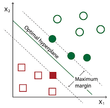
In order to explain the generalization behavior of algorithms minimizing a regularized risk we will introduce the luckiness framework. This framework is based on the assumption that the growth function will be estimated on the basis of a sample. Thus, it provides a-posteriori bounds; bounds which can only be evaluated after the training data has been seen. Finally, the chapter presents a PAC analysis for real-valued functions. Here, we take advantage of the fact that, in the case of linear classifiers, the classification is carried out by thresholding a realvalued function. The real-valued output, also referred to as the margin, allows us to define a scale sensitive version of the VC dimension which leads to tighter bounds on the expected risk. An appealing feature of the margin bound is that we can obtain nontrivial bounds even if the number of training samples is significantly less than the number of dimensions of feature space. Using a technique, which is known as the robustness trick, it will be demonstrated that the margin bound is also applicable if one allows for training error via a quadratic penalization of the diagonal of the Gram matrix.

统计代写|机器学习代写machine learning代考|Generative vs. Discriminative Models

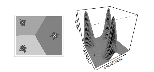
In Chapter 2 it was shown that a learning problem is given by a training sample $z=(\boldsymbol{x}, \boldsymbol{y})=\left(\left(x_{1}, y_{1}\right), \ldots,\left(x_{m}, y_{m}\right)\right) \in(\mathcal{X} \times \mathcal{Y})^{m}=\mathcal{Z}^{m}$, drawn iid according to some (unknown) probability measure $\mathbf{P}{\mathrm{Z}}=\mathbf{P}{\mathrm{XY}}$, and a loss $l: \mathcal{Y} \times \mathcal{Y} \rightarrow \mathbb{R}$, which defines how costly the prediction $h(x)$ is if the true output is $y$. Then, the goal is to find a deterministic function $h \in \mathcal{Y}^{\mathcal{X}}$ which expresses the dependency implicitly expressed by $\mathbf{P}{\mathbf{Z}}$ with minimal expected loss (risk) $R[h]=\mathbf{E}{X Y}[l(h(\mathrm{X}), \mathrm{Y})]$ while only using the given training sample $z$. We have already seen in the first part of this book that there exist two different algorithmical approaches to tackling this problem. We shall now try to study the two approaches more generally to see in what respect they are similar and in which aspects they differ.

1. In the generative (or parametric) statistics approach we restrict ourselves to a parameterized space $\mathcal{P}$ of measures for the space $\mathcal{Z}$, i.e., we model the data generation process. Hence, our model is given by ${ }^{1} \mathcal{P}=\left{\mathbf{P}{\mathrm{Z} \mid \mathbf{Q}=\theta} \mid \theta \in \mathcal{Q}\right}$, where $\theta$ should be understood as the parametric description of the measure $\mathbf{P}{\mathrm{Z} \mid \mathbf{Q}=\theta}$. With a fixed loss $l$ each measure $\mathbf{P}{\mathbf{Z} \mid \mathbf{Q}=\theta}$ implicitly defines a decision function $h{\theta}$,
   $$
   h_{\theta}(x)=\underset{y \in \mathcal{Y}}{\operatorname{argmin}} \mathbf{E}{Y \mid X=x, \mathbf{Q}=\theta}[l(y, Y)] \text {. } $$ In order to see that this function has minimal expected risk we note that $$ R{\theta}[h] \stackrel{\text { def }}{=} \mathbf{E}{\mathbf{X Y |} \mathbf{Q}=\theta}[l(h(\mathrm{X}), \mathrm{Y})]=\mathbf{E}{\mathbf{X} \mid \mathbf{Q}=\theta}\left[\mathbf{E}{Y \mid X=x, \mathbf{Q}=\theta}[l(h(x), \mathrm{Y})]\right] \text {, } $$ where $h{\theta}$ minimizes the expression in the innermost brackets. For the case of zeroone loss $l_{0-1}(h(x), y)=\mathbf{I}{h(x) \neq y}$ also defined in equation $(2.10)$, the function $h{\theta}$ reduces to
   $$
   h_{\theta}(x)=\underset{y \in \mathcal{Y}}{\operatorname{argmin}}\left(1-\mathbf{P}{\mathrm{Y} \mid \mathrm{X}=x, \mathbf{Q}=\theta}(y)\right)=\underset{y \in \mathcal{Y}}{\operatorname{argmax}} \mathbf{P}{\mathrm{Y} \mid \mathrm{X}=x, \mathbf{Q}=\theta}(y),
   $$
   which is known as the Bayes optimal decision based on $\mathbf{P}_{\mathrm{Z} \mid \mathbf{Q}=\theta}$.
2. In the discriminative, or machine learning, approach we restrict ourselves to a parameterized space $\mathcal{H} \subseteq \mathcal{Y}^{\mathcal{X}}$ of deterministic mappings $h$ from $\mathcal{X}$ to $\mathcal{Y}$. As a consequence, the model is given by $\mathcal{H}=\left{h_{\mathrm{w}}: \mathcal{X} \rightarrow \mathcal{Y} \mid \mathbf{w} \in \mathcal{W}\right}$, where $\mathbf{w}$ is the parameterization of single hypotheses $h_{\mathrm{w}}$. Note that this can also be interpreted as

a model of the conditional distribution of classes $y \in \mathcal{Y}$ given objects $x \in \mathcal{X}$ by assuming that $\mathbf{P}{Y \mid X=x, \mathcal{H}=h}=\mathbf{I}{y=h(x)}$. Viewed this way, the model $\mathcal{H}$ is a subset of the more general model $\mathcal{P}$ used in classical statistics.

The term generative refers to the fact that the model $\mathcal{P}$ contains different descriptions of the generation of the training sample $z$ (in terms of a probability measure). Similarly, the term discriminative refers to the fact that the model $\mathcal{H}$ consists of different descriptions of the discrimination of the sample $z$. We already know that a machine learning method selects one hypothesis $\mathcal{A}(z) \in \mathcal{H}$ given a training sample $z \in \mathcal{Z}^{m}$. The corresponding selection mechanism of a probability measure $\mathbf{P}_{\mathbf{z} \mid \mathbf{Q}=\theta}$ given the training sample $z$ is called an estimator.

统计代写|机器学习代写machine learning代考|Classical PAC and VC Analysis

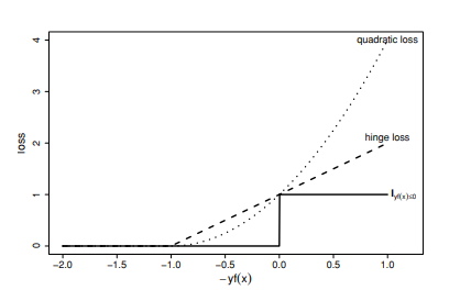
In the following three subsections we will only be concerned with the zero-one loss $l_{0-1}$ given by equation $(2.10)$. It should be noted that the results we will obtain can readily be generalized to loss function taking only a finite number values; the generalization to the case of real-valued loss functions conceptually similar but will not be discussed in this book (see Section $4.5$ for further references).

The general idea is to bound the probability of “bad training samples”, i.e., training samples $z \in \mathcal{Z}^{m}$ for which there exists a hypothesis $h \in \mathcal{H}$ where the deviation between the empirical risk $R_{\text {emp }}[h, z]$ and the expected risk $R[h]$ is larger than some prespecified $\varepsilon \in[0,1]$. Setting the probability of this to $\delta$ and solving for $\varepsilon$ gives the required generalization error bound. If we are only given a finite number $|\mathcal{H}|$ of hypotheses $h$ then such a bound is very easily obtained by a combination of Hoeffding’s inequality and the union bound.

Theorem 4.6 (VC bound for finite hypothesis spaces) Suppose we are given a hypothesis space $\mathcal{H}$ having a finite number of hypotheses, i.e., $|\mathcal{H}|<\infty$. Then, for any measure $\mathbf{P}{\mathrm{Z}}$, for all $\delta \in(0,1]$ and all training sample sizes $m \in \mathbb{N}$, with probability at least $1-\delta$ over the random draw of the training sample $z \in \mathcal{Z}^{m}$ we have $$ \mathbf{P}{Z^{w}}\left(\exists h \in \mathcal{H}:\left|R[h]-R_{\operatorname{emp}}[h, \mathbf{Z}]\right|>\varepsilon\right)<2 \cdot|\mathcal{H}| \cdot \exp \left(-2 m \varepsilon^{2}\right) $$ Proof Let $\mathcal{H}=\left\{h_{1}, \ldots, h_{|\mathcal{H}|}\right\}$. By an application of the union bound given in Theorem A.107 we know that $\mathbf{P}_{Z^{m}}\left(\exists h \in \mathcal{H}:\left|R[h]-R_{\text {emp }}[h, \mathbf{Z}]\right|>\varepsilon\right)$ is given by
$$
\mathbf{P}{Z^{m}}\left(\bigvee{i=1}^{|\mathcal{H}|}\left(\left|R\left[h_{i}\right]-R_{\mathrm{emp}}\left[h_{i}, \mathbf{Z}\right]\right|>\varepsilon\right)\right) \leq \sum_{i=1}^{|\mathcal{H}|} \mathbf{P}{Z^{m}}\left(\left|R\left[h{i}\right]-R_{\mathrm{emp}}\left[h_{i}, \mathbf{Z}\right]\right|>\varepsilon\right) .
$$

机器学习代写

统计代写|机器学习代写machine learning代考|Mathematical Models of Learning

本章介绍了不同的学习数学模型。学习的数学模型的优点是它为学习算法的泛化能力提供了界限。它还指示哪些量负责泛化。因此，该理论激发了新的学习算法。在简要介绍了经典的参数统计学习方法之后，本章介绍了 PAC 和 VC 模型。这些模型直接研究预期风险的收敛性，而不是绕开潜在概率测度的收敛性。这个框架中的基本量是增长函数，其上限是一个整数总结，称为 VC 维度。通过经典的结构风险最小化，一种-priori bounds，即对于固定训练误差其值相同的边界。

为了解释最小化正则化风险的算法的泛化行为，我们将介绍幸运框架。该框架基于这样的假设，即增长函数将根据样本进行估计。因此，它提供了后验界限；只有在看到训练数据后才能评估的界限。最后，本章介绍了实值函数的 PAC 分析。在这里，我们利用了这样一个事实，即在线性分类器的情况下，分类是通过对实值函数进行阈值化来执行的。实值输出，也称为边际，允许我们定义 VC 维度的规模敏感版本，从而对预期风险进行更严格的限制。边缘界限的一个吸引人的特点是，即使训练样本的数量明显少于特征空间的维数，我们也可以获得非平凡的界限。使用一种称为鲁棒性技巧的技术，将证明如果通过对 Gram 矩阵的对角线的二次惩罚来允许训练误差，则边缘界限也是适用的。

统计代写|机器学习代写machine learning代考|Generative vs. Discriminative Models

在第 2 章中，我们展示了一个学习问题是由一个训练样本给出的和=(X,是)=((X1,是1),…,(X米,是米))∈(X×是)米=从米，根据一些（未知）概率测度绘制独立同分布磷从=磷X是, 和损失l:是×是→R，它定义了预测的成本H(X)是如果真正的输出是是. 然后，目标是找到一个确定性函数H∈是X它表达了隐式表达的依赖关系磷从以最小的预期损失（风险）R[H]=和X是[l(H(X),是)]仅使用给定的训练样本和. 我们在本书的第一部分已经看到，存在两种不同的算法方法来解决这个问题。我们现在将尝试更广泛地研究这两种方法，看看它们在哪些方面相似，在哪些方面不同。

1. 在生成（或参数）统计方法中，我们将自己限制在参数化空间中磷空间措施从，即我们对数据生成过程进行建模。因此，我们的模型由下式给出{ }^{1} \mathcal{P}=\left{\mathbf{P}{\mathrm{Z}\mid\mathbf{Q}=\theta}\mid\theta\in\mathcal{Q}\right } }{ }^{1} \mathcal{P}=\left{\mathbf{P}{\mathrm{Z}\mid\mathbf{Q}=\theta}\mid\theta\in\mathcal{Q}\right } }， 在哪里θ应该理解为度量的参数化描述磷从∣问=θ. 有固定损失l每个措施磷从∣问=θ隐式定义决策函数Hθ,
   Hθ(X)=精氨酸是∈是和是∣X=X,问=θ[l(是,是)]. 为了看到这个函数具有最小的预期风险，我们注意到Rθ[H]= 定义 和X是|问=θ[l(H(X),是)]=和X∣问=θ[和是∣X=X,问=θ[l(H(X),是)]], 在哪里Hθ最小化最里面的括号中的表达式。对于 zeroone loss 的情况l0−1(H(X),是)=一世H(X)≠是也在等式中定义(2.10)， 功能Hθ减少到
   Hθ(X)=精氨酸是∈是(1−磷是∣X=X,问=θ(是))=最大参数是∈是磷是∣X=X,问=θ(是),
   这被称为基于贝叶斯最优决策磷从∣问=θ.
2. 在判别式或机器学习方法中，我们将自己限制在参数化空间中H⊆是X确定性映射H从X到是. 因此，模型由下式给出\mathcal{H}=\left{h_{\mathrm{w}}: \mathcal{X} \rightarrow \mathcal{Y} \mid \mathbf{w} \in \mathcal{W}\right}\mathcal{H}=\left{h_{\mathrm{w}}: \mathcal{X} \rightarrow \mathcal{Y} \mid \mathbf{w} \in \mathcal{W}\right}， 在哪里在是单个假设的参数化H在. 请注意，这也可以解释为

类的条件分布模型是∈是给定对象X∈X通过假设 $\mathbf{P} {Y \mid X=x, \mathcal{H}=h}=\mathbf{I} {y=h(x)}.在一世和在和d吨H一世s在一种是,吨H和米这d和l\数学{H}一世s一种s在bs和吨这F吨H和米这r和G和n和r一种l米这d和l\mathcal{P}$ 用于经典统计。

术语生成是指模型磷包含对训练样本生成的不同描述和（就概率测度而言）。同样，判别性一词是指模型H由对样本辨别力的不同描述组成和. 我们已经知道机器学习方法选择一个假设一种(和)∈H给定一个训练样本和∈从米. 概率测度的相应选择机制磷和∣问=θ给定训练样本和称为估计器。

统计代写|机器学习代写machine learning代考|Classical PAC and VC Analysis

在以下三个小节中，我们将只关注零一损失l0−1由方程给出(2.10). 应该注意的是，我们将获得的结果可以很容易地推广到仅采用有限数值的损失函数；在概念上相似的实值损失函数的情况下的推广，但不会在本书中讨论（见第4.5供进一步参考）。

总体思路是对“坏训练样本”的概率进行约束，即训练样本和∈从米存在一个假设H∈H其中经验风险之间的偏差R雇员 [H,和]和预期风险R[H]大于某些预先指定的e∈[0,1]. 将此概率设置为d并解决e给出所需的泛化误差界. 如果我们只得到一个有限的数字|H|假设H那么通过 Hoeffding 不等式和联合界限的组合很容易获得这样的界限。

定理 4.6（有限假设空间的 VC 界）假设给定一个假设空间H有有限数量的假设，即|H|<∞. 然后，对于任何度量磷从， 对全部d∈(0,1]和所有训练样本大小米∈ñ, 至少有概率1−d在训练样本的随机抽取上和∈从米我们有磷从在(∃H∈H:|R[H]−R雇员[H,从]|>e)<2⋅|H|⋅经验⁡(−2米e2)证明让H={H1,…,H|H|}. 通过应用定理 A.107 中给出的联合界限，我们知道磷从米(∃H∈H:|R[H]−R雇员 [H,从]|>e)是（谁）给的
磷从米(⋁一世=1|H|(|R[H一世]−R和米p[H一世,从]|>e))≤∑一世=1|H|磷从米(|R[H一世]−R和米p[H一世,从]|>e).

统计代写请认准statistics-lab™. statistics-lab™为您的留学生涯保驾护航。

金融工程代写

金融工程是使用数学技术来解决金融问题。金融工程使用计算机科学、统计学、经济学和应用数学领域的工具和知识来解决当前的金融问题，以及设计新的和创新的金融产品。

非参数统计代写

非参数统计指的是一种统计方法，其中不假设数据来自于由少数参数决定的规定模型；这种模型的例子包括正态分布模型和线性回归模型。

广义线性模型代考

广义线性模型（GLM）归属统计学领域，是一种应用灵活的线性回归模型。该模型允许因变量的偏差分布有除了正态分布之外的其它分布。

术语 广义线性模型（GLM）通常是指给定连续和/或分类预测因素的连续响应变量的常规线性回归模型。它包括多元线性回归，以及方差分析和方差分析（仅含固定效应）。

有限元方法代写

有限元方法（FEM）是一种流行的方法，用于数值解决工程和数学建模中出现的微分方程。典型的问题领域包括结构分析、传热、流体流动、质量运输和电磁势等传统领域。

有限元是一种通用的数值方法，用于解决两个或三个空间变量的偏微分方程（即一些边界值问题）。为了解决一个问题，有限元将一个大系统细分为更小、更简单的部分，称为有限元。这是通过在空间维度上的特定空间离散化来实现的，它是通过构建对象的网格来实现的：用于求解的数值域，它有有限数量的点。边界值问题的有限元方法表述最终导致一个代数方程组。该方法在域上对未知函数进行逼近。[1] 然后将模拟这些有限元的简单方程组合成一个更大的方程系统，以模拟整个问题。然后，有限元通过变化微积分使相关的误差函数最小化来逼近一个解决方案。

tatistics-lab作为专业的留学生服务机构，多年来已为美国、英国、加拿大、澳洲等留学热门地的学生提供专业的学术服务，包括但不限于Essay代写，Assignment代写，Dissertation代写，Report代写，小组作业代写，Proposal代写，Paper代写，Presentation代写，计算机作业代写，论文修改和润色，网课代做，exam代考等等。写作范围涵盖高中，本科，研究生等海外留学全阶段，辐射金融，经济学，会计学，审计学，管理学等全球99%专业科目。写作团队既有专业英语母语作者，也有海外名校硕博留学生，每位写作老师都拥有过硬的语言能力，专业的学科背景和学术写作经验。我们承诺100%原创，100%专业，100%准时，100%满意。

随机分析代写

随机微积分是数学的一个分支，对随机过程进行操作。它允许为随机过程的积分定义一个关于随机过程的一致的积分理论。这个领域是由日本数学家伊藤清在第二次世界大战期间创建并开始的。

时间序列分析代写

随机过程，是依赖于参数的一组随机变量的全体，参数通常是时间。 随机变量是随机现象的数量表现，其时间序列是一组按照时间发生先后顺序进行排列的数据点序列。通常一组时间序列的时间间隔为一恒定值（如1秒，5分钟，12小时，7天，1年），因此时间序列可以作为离散时间数据进行分析处理。研究时间序列数据的意义在于现实中，往往需要研究某个事物其随时间发展变化的规律。这就需要通过研究该事物过去发展的历史记录，以得到其自身发展的规律。

回归分析代写

多元回归分析渐进（Multiple Regression Analysis Asymptotics）属于计量经济学领域，主要是一种数学上的统计分析方法，可以分析复杂情况下各影响因素的数学关系，在自然科学、社会和经济学等多个领域内应用广泛。

MATLAB代写

MATLAB 是一种用于技术计算的高性能语言。它将计算、可视化和编程集成在一个易于使用的环境中，其中问题和解决方案以熟悉的数学符号表示。典型用途包括：数学和计算算法开发建模、仿真和原型制作数据分析、探索和可视化科学和工程图形应用程序开发，包括图形用户界面构建MATLAB 是一个交互式系统，其基本数据元素是一个不需要维度的数组。这使您可以解决许多技术计算问题，尤其是那些具有矩阵和向量公式的问题，而只需用 C 或 Fortran 等标量非交互式语言编写程序所需的时间的一小部分。MATLAB 名称代表矩阵实验室。MATLAB 最初的编写目的是提供对由 LINPACK 和 EISPACK 项目开发的矩阵软件的轻松访问，这两个项目共同代表了矩阵计算软件的最新技术。MATLAB 经过多年的发展，得到了许多用户的投入。在大学环境中，它是数学、工程和科学入门和高级课程的标准教学工具。在工业领域，MATLAB 是高效研究、开发和分析的首选工具。MATLAB 具有一系列称为工具箱的特定于应用程序的解决方案。对于大多数 MATLAB 用户来说非常重要，工具箱允许您学习和应用专业技术。工具箱是 MATLAB 函数（M 文件）的综合集合，可扩展 MATLAB 环境以解决特定类别的问题。可用工具箱的领域包括信号处理、控制系统、神经网络、模糊逻辑、小波、仿真等。

R语言代写	问卷设计与分析代写
PYTHON代写	回归分析与线性模型代写
MATLAB代写	方差分析与试验设计代写
STATA代写	机器学习/统计学习代写
SPSS代写	计量经济学代写
EVIEWS代写	时间序列分析代写
EXCEL代写	深度学习代写
SQL代写	各种数据建模与可视化代写

如果你也在 怎样代写机器学习machine learning这个学科遇到相关的难题，请随时右上角联系我们的24/7代写客服。

机器学习是对计算机算法的研究，这些算法可以通过经验和使用数据来自动改进。机器学习算法基于样本数据（称为训练数据）建立模型，以便在没有明确编程的情况下做出预测或决定。机器学习算法被广泛用于各种应用中，如医学、电子邮件过滤、语音识别和计算机视觉，在这些应用中，开发传统算法来执行所需的任务是困难的或不可行的。

statistics-lab™ 为您的留学生涯保驾护航 在代写机器学习machine learning方面已经树立了自己的口碑, 保证靠谱, 高质且原创的统计Statistics代写服务。我们的专家在代写机器学习machine learning代写方面经验极为丰富，各种代写机器学习machine learning相关的作业也就用不着说。

我们提供的机器学习machine learning及其相关学科的代写，服务范围广, 其中包括但不限于:

• Statistical Inference 统计推断
• Statistical Computing 统计计算
• Advanced Probability Theory 高等概率论
• Advanced Mathematical Statistics 高等数理统计学
• (Generalized) Linear Models 广义线性模型
• Statistical Machine Learning 统计机器学习
• Longitudinal Data Analysis 纵向数据分析
• Foundations of Data Science 数据科学基础

统计代写|机器学习代写machine learning代考|The Relevance Vector Machine

In the last section we saw that a direct application of Bayesian ideas to the problem of regression estimation yields efficient algorithms known as Gaussian processes. In this section we will carry out the same analysis with a slightly refined prior $\mathbf{P}{\mathrm{w}}$ on linear functions $f{\mathrm{w}}$ in terms of their weight vectors $\mathbf{w} \in \mathcal{K} \subseteq \ell_{2}^{n}$. As we will

see in Section $5.2$ an important quantity in the study of the generalization error is the sparsity $|\mathbf{w}|_{0}=\sum_{i=1}^{n} \mathbf{I}{w{i} \neq 0}$ or $|\boldsymbol{\alpha}|_{0}$ of the weight vector or the vector of expansion coefficients, respectively. In particular, it is shown that the expected risk of the classifier $f_{\mathrm{w}}$ learned from a training sample $z \in \mathcal{Z}^{m}$ is, with high probability over the random draw of $z$, as small as $\approx \frac{\boldsymbol{w}{0}}{n}$ or $\frac{|\alpha|{0}}{m}$, where $n$ is the dimensionality of the feature space $\mathcal{K}$ and $\mathbf{w}=\sum_{i=1}^{m} \alpha_{i} \mathbf{x}{i}=\mathbf{X}^{\prime} \alpha$. These results suggest favoring weight vectors with a small number of non-zero coefficients. One way to achieve this is to modify the prior in equation (3.8), giving $\mathbf{P}{\mathbf{W}}=\operatorname{Normal}(\mathbf{0}, \boldsymbol{\Theta})$,
where $\boldsymbol{\Theta}=\operatorname{diag}(\theta)$ and $\theta=\left(\theta_{1}, \ldots, \theta_{n}\right)^{\prime} \in\left(\mathbb{R}^{+}\right)^{n}$ is assumed known. The idea behind this prior is similar to the idea of automatic relevance determination given in Example 3.12. By considering $\theta_{i} \rightarrow 0$ we see that the only possible value for the $i$ th component of the weight vector $w$ is 0 and, therefore, even when considering the Bayesian prediction $B a y e s_{z}$ the $i$ th component is set to zero. In order to make inference we consider the likelihood model given in equation (3.9), that is, we assume that the target values $t=\left(t_{1}, \ldots, t_{m}\right) \in \mathbb{R}^{m}$ are normally distributed with mean $\left\langle\mathbf{x}{i}, \mathbf{w}\right\rangle$ and variance $\sigma{t}^{2}$. Using Theorem A.28 it follows that the posterior measure over weight vectors $\mathbf{w}$ is again Gaussian, i.e.,
$\mathbf{P}{W \mid} \mathrm{X}^{m}=x, \mathrm{~T}^{\mathrm{m}}=t=\operatorname{Normal}(\boldsymbol{\mu}, \boldsymbol{\Sigma})$ where the posterior covariance $\mathbf{\Sigma} \in \mathbb{R}^{n \times n}$ and mean $\mu \in \mathbb{R}^{n}$ are given by $$ \boldsymbol{\Sigma}=\left(\sigma{t}^{-2} \mathbf{X}^{\prime} \mathbf{X}+\boldsymbol{\Theta}^{-1}\right)^{-1}, \quad \boldsymbol{\mu}=\sigma_{t}^{-2} \boldsymbol{\Sigma} \mathbf{X}^{\prime} \boldsymbol{t}=\left(\mathbf{X}^{\prime} \mathbf{X}+\sigma_{t}^{2} \mathbf{\Theta}^{-1}\right)^{-1} \mathbf{X}^{\prime} \boldsymbol{t}
$$
As described in the last section, the Bayesian prediction at a new test object $x \in \mathcal{X}$ is given by $B a$ ayes $_{z}(x)=\langle\mathbf{x}, \boldsymbol{\mu}\rangle$. Since we assumed that many of the $\theta_{i}$ are zero, i.e., the effective number $n_{\text {eff }}=|\theta|_{0}$ of features $\phi_{i}: \mathcal{X} \rightarrow \mathbb{R}$ is small, it follows that $\boldsymbol{\Sigma}$ and $\boldsymbol{\mu}$ are easy to calculate ${ }^{7}$. The interesting question is: Given a training sample $z=(\boldsymbol{x}, \boldsymbol{t}) \in(\mathcal{X} \times \mathbb{R})^{m}$, how can we “learn” the sparse vector $\boldsymbol{\theta}=\left(\theta_{1}, \ldots, \theta_{n}\right)^{\prime} ?$

统计代写|机器学习代写machine learning代考|Bayes Point Machines

The algorithms introduced in the last two sections solve the classification learning problem by taking a “detour” via the regression estimation problem. For each training object it is assumed that we have prior knowledge $\mathbf{P}{\mathbf{w}}$ about the latent variables $\mathrm{T}{i}$ corresponding to the logit transformation of the probability of $x_{i}$ being from the observed class $y_{i}$. This is a quite cumbersome assumption as we are unable to directly express prior knowledge on observed quantities such as the classes $\boldsymbol{y} \in \mathcal{Y}^{m}={-1,+1}^{m}$. In this section we are going to consider an algorithm which results from a direct modeling of the classes.

Let us start by defining the prior $\mathbf{P}{\mathbf{W}}$. In the classification case we note that, for any $\lambda>0$, the weight vectors $w$ and $\lambda w$ perform the same classification because $\operatorname{sign}(\langle\mathbf{x}, \mathbf{w}\rangle)=\operatorname{sign}(\langle\mathbf{x}, \lambda \mathbf{w}\rangle)$. As a consequence we consider only weight vectors of unit length, i.e., w $\in \mathcal{W}, \mathcal{W}={\mathbf{w} \in \mathcal{K} \mid|\mathbf{w}|=1}$ (see also Section 2.1). In the absence of any prior knowledge we assume a uniform prior measure $\mathbf{P}{\mathbf{W}}$ over the unit hypersphere $\mathcal{W}$. An argument in favor of the uniform prior is that the belief in the weight vector $w$ should be equal to the belief in the weight vector $-\mathbf{w}$

under the assumption of equal class probabilities $\mathbf{P}{\curlyvee}(-1)$ and $\mathbf{P}{\curlyvee}(+1)$. Since the classification $\mathbf{y}{-\mathbf{w}}=\left(\operatorname{sign}\left(\left\langle\mathbf{x}{1},-\mathbf{w}\right\rangle\right), \ldots, \operatorname{sign}\left(\left\langle\mathbf{x}{m},-\mathbf{w}\right\rangle\right)\right)$ of the weight vector $-\mathbf{w}$ at the training sample $z \in \mathcal{Z}^{m}$ equals the negated classification $-\mathbf{y}{\mathbf{w}}=$ $-\left(\operatorname{sign}\left(\left\langle\mathbf{x}{1}, \mathbf{w}\right\rangle\right), \ldots, \operatorname{sign}\left(\left\langle\mathbf{x}{m}, \mathbf{w}\right\rangle\right)\right)$ of $\mathbf{w}$ it follows that the assumption of equal belief in $\mathbf{w}$ and $-\mathbf{w}$ corresponds to assuming that $\mathbf{P}{\mathbf{Y}}(-1)=\mathbf{P}{\mathbf{Y}}(+1)=\frac{1}{2}$.

In order to derive an appropriate likelihood model, let us assume that there is no noise on the classifications, that is, we shall use the PAC-likelihood $l_{\mathrm{PAC}}$ as given in Definition 3.3. Note that such a likelihood model corresponds to using the zeroone loss $I_{0-1}$ in the machine learning scenario (see equations $(2.10)$ and $(3.2)$ ). According to Bayes’ theorem it follows that the posterior belief in weight vectors (and therefore in classifiers) is given by
$$
\begin{aligned}
f_{W \mid Z^{m}=z}(w) &=\frac{P_{Y^{m} \mid X^{m}=x, W=w}(y) f_{W}(w)}{P_{Y^{m} \mid X^{m}=x}(y)} \
&= \begin{cases}\frac{1}{P_{W}(V(z))} & \text { if } w \in V(z) \
0 & \text { otherwise }\end{cases}
\end{aligned}
$$
The set $V(z) \subseteq \mathcal{W}$ is called version space and is the set of all weight vectors that parameterize classifiers which classify all the training objects correctly (see also Definition 2.12). Due to the PAC-likelihood, any weight vector which does not have this property is “cut-off” resulting in a uniform posterior measure $\mathbf{P}{\mathbf{W} \mid \mathbf{Z}^{m}=z}$ over version space. Given a new test object $x \in \mathcal{X}$ we can compute the predictive distribution $\mathbf{P}{Y \mid X=x, Z^{m}=z}$ of the class $y$ at $x \in \mathcal{X}$ by
$$
\mathbf{P}{\mathrm{Y} \mid \mathrm{X}=x, Z^{w}=z}(y)=\mathbf{P}{\mathrm{W} \mid \mathbf{Z}^{m}=z}(\operatorname{sign}(\langle\mathbf{x}, \mathbf{W}\rangle)=y) .
$$
The Bayes classification strategy based on $\mathbf{P}{\mathrm{Y} \mid \mathrm{X}=x, \mathrm{Z}^{\mathrm{m}}=z}$ decides on the class with the larger probability. An appealing feature of the two class case $\mathcal{Y}={-1,+1}$ is that this decision can also be written as $\operatorname{Bayes}{z}(x)=\operatorname{sign}\left(\mathbf{E}_{\mathbf{W} \mid \mathbf{Z}^{m}=z}[\operatorname{sign}(\langle\mathbf{x}, \mathbf{W}\rangle)]\right)$,
that is, the Bayes classification strategy effectively performs majority voting involving all version space classifiers. The difficulty with the latter expression is that we cannot analytically compute the expectation as this requires efficient integration of a convex body on a hypersphere (see also Figure $2.1$ and $2.8$ ). Hence, we approximate the Bayes classification strategy by a single classifier.

统计代写|机器学习代写machine learning代考|Estimating the Bayes Point

The main idea in computing the center of mass of version space is to replace the analytical integral by a sum over randomly drawn classifiers, i.e.,
$$
\mathbf{w}{\mathrm{cm}}=\mathbf{E}{W \mid \mathbf{Z}^{\mathrm{w}}=z}[\mathbf{W}] \approx \frac{1}{K} \sum_{i=1}^{K} \mathbf{w}{i} \quad \mathbf{w}{i} \sim \mathbf{P}{\mathbf{W} \mid \mathbf{Z}^{m}=z} $$ Such methods are known as Monte-Carlo methods and have proven to be successful in practice. A difficulty we encounter with this approach is in obtaining samples $\mathbf{w}{i}$ drawn according to the distribution $\mathbf{P}{\mathbf{W} \mid \mathrm{Z}^{\mathrm{m}}=z \text {. Recalling }}$ that $\mathbf{P}{\mathrm{W} / \mathrm{Z}^{\mathrm{m}}=z}$ is uniform in a convex polyhedra on the surface of hypersphere in feature space we see that it is quite difficult to directly sample from it. A commonly used approach to this problem is to approximate the sampling distribution $\mathbf{P}{\mathrm{W} \mid \mathrm{Z}^{\mathrm{m}}=z}$ by a Markov chain. A Markov chain is fully specified by a probability distribution $\mathbf{P}{\mathrm{W}{1} \mathbf{W}{2}}$ where $f_{W_{1}} w_{2}\left(\left(w_{1}, w_{2}\right)\right)$ is the “transition” probability for progressing from a randomly drawn weight vector $\mathbf{w}{1}$ to another weight vector $\mathbf{w}{2}$. Sampling from the Markov chain involves iteratively drawing a new weight vector $w_{i+1}$ by sampling from $\mathbf{P}{\mathrm{W}{2} \mid \mathrm{W}{1}=\mathrm{w}{i} .}$ The Markov chain is called ergodic w.r.t. $\mathbf{P}{\mathbf{W} \mid \mathrm{Z}^{\mathrm{w}}=z}$ if the limiting distribution of this sampling process is $\mathbf{P}{\mathbf{w} \mid \mathbf{Z}^{m}=z}$ regardless of our choice of $\mathbf{w}{0}$. Then, it suffices to start with a random weight vector $w{0} \in \mathcal{W}$ and at each step, to obtain a new sample $\mathbf{w}{i} \in \mathcal{W}$ drawn according to $\mathbf{P}{\mathbf{w}{2} \mid \mathbf{w}{1}=\mathbf{w}{i-1} .}$. The combination of these two techniques has become known as the Markov-Chain-Monte-Carlo (MCMC) method for estimating the expectation $\mathbf{E}{\mathbf{W} \mid \mathbf{Z}^{w}=z}[\mathbf{W}]$.

We now outline an MCMC algorithm for approximating the Bayes point by the center of mass of version space $V(z)$ (the whole pseudo code is given on page 330). Since it is difficult to generate weight vectors that parameterize classifiers consistent with the whole training sample $z \in \mathcal{Z}^{m}$ we average over the trajectory of a ball which is placed inside version space and bounced like a billiard ball. As a consequence we call this MCMC method the kernel billiard. We express each position $\mathbf{b} \in \mathcal{W}$ of the ball and each estimate $\mathbf{w}{i} \in \mathcal{W}$ of the center of mass of $V(z)$ as a linear combination of the mapped training objects, i.e., $$ \mathbf{w}=\sum{i=1}^{m} \alpha_{i} \mathbf{x}{i}, \quad \mathbf{b}=\sum{i=1}^{m} \gamma_{i} \mathbf{x}_{i}, \quad \alpha \in \mathbb{R}^{m}, \quad \boldsymbol{\gamma} \in \mathbb{R}^{m}
$$

机器学习代写

统计代写|机器学习代写machine learning代考|The Relevance Vector Machine

在上一节中，我们看到将贝叶斯思想直接应用于回归估计问题会产生称为高斯过程的高效算法。在本节中，我们将使用稍微改进的先验进行相同的分析磷在关于线性函数F在就他们的权重向量而言在∈ķ⊆ℓ2n. 正如我们将

见第5.2泛化误差研究中的一个重要量是稀疏度|在|0=∑一世=1n一世在一世≠0或者|一种|0分别为权重向量或膨胀系数向量。特别是，它表明分类器的预期风险F在从训练样本中学习和∈从米是，在随机抽取的概率很高和， 一样小≈在0n或者|一种|0米， 在哪里n是特征空间的维数ķ和在=∑一世=1米一种一世X一世=X′一种. 这些结果表明偏爱具有少量非零系数的权重向量。实现这一点的一种方法是修改等式（3.8）中的先验，给出磷在=普通的⁡(0,θ),
其中θ=诊断⁡(θ)和θ=(θ1,…,θn)′∈(R+)n假定已知。这个先验背后的想法类似于示例 3.12 中给出的自动相关性确定的想法。通过考虑θ一世→0我们看到唯一可能的值一世权重向量的第 th 分量在为 0，因此，即使考虑贝叶斯预测乙一种是和s和这一世th 分量设置为零。为了进行推断，我们考虑方程（3.9）中给出的似然模型，即我们假设目标值吨=(吨1,…,吨米)∈R米均值正态分布⟨X一世,在⟩和方差σ吨2. 使用定理 A.28 可以得出对权重向量的后验测度在又是高斯分布，即
磷在∣X米=X, 吨米=吨=普通的⁡(μ,Σ)其中后协方差Σ∈Rn×n和意思μ∈Rn由Σ=(σ吨−2X′X+θ−1)−1,μ=σ吨−2ΣX′吨=(X′X+σ吨2θ−1)−1X′吨
如上一节所述，新测试对象的贝叶斯预测X∈X是（谁）给的乙一种是的和(X)=⟨X,μ⟩. 由于我们假设许多θ一世为零，即有效数n效果 =|θ|0特征φ一世:X→R很小，因此Σ和μ很容易计算7. 有趣的问题是：给定一个训练样本和=(X,吨)∈(X×R)米，我们如何“学习”稀疏向量θ=(θ1,…,θn)′?

统计代写|机器学习代写machine learning代考|Bayes Point Machines

最后两节介绍的算法通过回归估计问题“绕道”解决了分类学习问题。对于每个训练对象，假设我们有先验知识磷在关于潜变量吨一世对应概率的logit变换X一世来自被观察的班级是一世. 这是一个相当繁琐的假设，因为我们无法直接表达关于观测量的先验知识，例如类是∈是米=−1,+1米. 在本节中，我们将考虑一种由类的直接建模产生的算法。

让我们从定义先验开始磷在. 在分类情况下，我们注意到，对于任何λ>0, 权重向量在和λ在执行相同的分类，因为符号⁡(⟨X,在⟩)=符号⁡(⟨X,λ在⟩). 因此，我们只考虑单位长度的权重向量，即 w∈在,在=在∈ķ∣|在|=1（另见第 2.1 节）。在没有任何先验知识的情况下，我们假设一个统一的先验测量磷在在单位超球面上在. 支持统一先验的一个论据是对权重向量的信念在应该等于对权重向量的置信度−在

在相同类别概率的假设下磷⋎(−1)和磷⋎(+1). 由于分类是−在=(符号⁡(⟨X1,−在⟩),…,符号⁡(⟨X米,−在⟩))权重向量的−在在训练样本和∈从米等于否定分类−是在= −(符号⁡(⟨X1,在⟩),…,符号⁡(⟨X米,在⟩))的在因此，平等信念的假设在和−在对应于假设磷是(−1)=磷是(+1)=12.

为了推导出一个合适的似然模型，让我们假设分类中没有噪声，也就是说，我们将使用 PAC-likelihoodl磷一种C如定义 3.3 中给出的。请注意，这样的似然模型对应于使用 zeroone 损失一世0−1在机器学习场景中（见方程式(2.10)和(3.2)）。根据贝叶斯定理，权重向量（以及分类器）的后验信念由下式给出
F在∣从米=和(在)=磷是米∣X米=X,在=在(是)F在(在)磷是米∣X米=X(是) ={1磷在(在(和)) 如果 在∈在(和) 0 除此以外 
套装在(和)⊆在被称为版本空间，它是参数化分类器的所有权重向量的集合，这些分类器正确分类所有训练对象（另见定义 2.12）。由于 PAC 似然，任何不具有此属性的权重向量都会被“截断”，从而产生统一的后验度量磷在∣从米=和超过版本空间。给定一个新的测试对象X∈X我们可以计算预测分布磷是∣X=X,从米=和班级的是在X∈X经过
磷是∣X=X,从在=和(是)=磷在∣从米=和(符号⁡(⟨X,在⟩)=是).
贝叶斯分类策略基于磷是∣X=X,从米=和决定概率较大的类别。二类案件的一个吸引人的特点是=−1,+1是这个决定也可以写成贝叶斯⁡和(X)=符号⁡(和在∣从米=和[符号⁡(⟨X,在⟩)])，
即贝叶斯分类策略有效地执行涉及所有版本空间分类器的多数投票。后一个表达式的困难在于我们无法解析地计算期望，因为这需要在超球面上有效集成凸体（另请参见图2.1和2.8）。因此，我们通过单个分类器来近似贝叶斯分类策略。

统计代写|机器学习代写machine learning代考|Estimating the Bayes Point

计算版本空间的质心的主要思想是用随机绘制的分类器上的和来代替解析积分，即
在C米=和在∣从在=和[在]≈1ķ∑一世=1ķ在一世在一世∼磷在∣从米=和这种方法被称为蒙特卡洛方法，并已在实践中证明是成功的。我们使用这种方法遇到的一个困难是获取样本在一世根据分布绘制磷在∣从米=和. 召回 那磷在/从米=和在特征空间的超球面上的凸多面体中是均匀的，我们看到很难直接从中采样。解决这个问题的常用方法是近似采样分布磷在∣从米=和通过马尔可夫链。马尔可夫链完全由概率分布指定磷在1在2在哪里F在1在2((在1,在2))是从随机绘制的权重向量进行的“转移”概率在1到另一个权重向量在2. 从马尔可夫链采样涉及迭代绘制一个新的权重向量在一世+1通过抽样磷在2∣在1=在一世.马尔可夫链称为遍历 wrt磷在∣从在=和如果这个抽样过程的极限分布是磷在∣从米=和无论我们选择什么在0. 然后，从一个随机权重向量开始就足够了在0∈在并且在每一步，获得一个新的样本在一世∈在根据绘制磷在2∣在1=在一世−1.. 这两种技术的结合已被称为用于估计期望的马尔可夫链蒙特卡罗 (MCMC) 方法和在∣从在=和[在].

我们现在概述一个 MCMC 算法，用于通过版本空间的质心来逼近贝叶斯点在(和)（整个伪代码在第 330 页给出）。由于很难生成与整个训练样本一致的参数化分类器的权重向量和∈从米我们对放置在版本空间内并像台球一样弹跳的球的轨迹进行平均。因此，我们将此 MCMC 方法称为内核台球。我们表达每一个立场b∈在球和每个估计在一世∈在的质心在(和)作为映射训练对象的线性组合，即在=∑一世=1米一种一世X一世,b=∑一世=1米C一世X一世,一种∈R米,C∈R米

统计代写请认准statistics-lab™. statistics-lab™为您的留学生涯保驾护航。

金融工程代写

金融工程是使用数学技术来解决金融问题。金融工程使用计算机科学、统计学、经济学和应用数学领域的工具和知识来解决当前的金融问题，以及设计新的和创新的金融产品。

非参数统计代写

非参数统计指的是一种统计方法，其中不假设数据来自于由少数参数决定的规定模型；这种模型的例子包括正态分布模型和线性回归模型。

广义线性模型代考

广义线性模型（GLM）归属统计学领域，是一种应用灵活的线性回归模型。该模型允许因变量的偏差分布有除了正态分布之外的其它分布。

术语 广义线性模型（GLM）通常是指给定连续和/或分类预测因素的连续响应变量的常规线性回归模型。它包括多元线性回归，以及方差分析和方差分析（仅含固定效应）。

有限元方法代写

有限元方法（FEM）是一种流行的方法，用于数值解决工程和数学建模中出现的微分方程。典型的问题领域包括结构分析、传热、流体流动、质量运输和电磁势等传统领域。

有限元是一种通用的数值方法，用于解决两个或三个空间变量的偏微分方程（即一些边界值问题）。为了解决一个问题，有限元将一个大系统细分为更小、更简单的部分，称为有限元。这是通过在空间维度上的特定空间离散化来实现的，它是通过构建对象的网格来实现的：用于求解的数值域，它有有限数量的点。边界值问题的有限元方法表述最终导致一个代数方程组。该方法在域上对未知函数进行逼近。[1] 然后将模拟这些有限元的简单方程组合成一个更大的方程系统，以模拟整个问题。然后，有限元通过变化微积分使相关的误差函数最小化来逼近一个解决方案。

tatistics-lab作为专业的留学生服务机构，多年来已为美国、英国、加拿大、澳洲等留学热门地的学生提供专业的学术服务，包括但不限于Essay代写，Assignment代写，Dissertation代写，Report代写，小组作业代写，Proposal代写，Paper代写，Presentation代写，计算机作业代写，论文修改和润色，网课代做，exam代考等等。写作范围涵盖高中，本科，研究生等海外留学全阶段，辐射金融，经济学，会计学，审计学，管理学等全球99%专业科目。写作团队既有专业英语母语作者，也有海外名校硕博留学生，每位写作老师都拥有过硬的语言能力，专业的学科背景和学术写作经验。我们承诺100%原创，100%专业，100%准时，100%满意。

随机分析代写

随机微积分是数学的一个分支，对随机过程进行操作。它允许为随机过程的积分定义一个关于随机过程的一致的积分理论。这个领域是由日本数学家伊藤清在第二次世界大战期间创建并开始的。

时间序列分析代写

随机过程，是依赖于参数的一组随机变量的全体，参数通常是时间。 随机变量是随机现象的数量表现，其时间序列是一组按照时间发生先后顺序进行排列的数据点序列。通常一组时间序列的时间间隔为一恒定值（如1秒，5分钟，12小时，7天，1年），因此时间序列可以作为离散时间数据进行分析处理。研究时间序列数据的意义在于现实中，往往需要研究某个事物其随时间发展变化的规律。这就需要通过研究该事物过去发展的历史记录，以得到其自身发展的规律。

回归分析代写

多元回归分析渐进（Multiple Regression Analysis Asymptotics）属于计量经济学领域，主要是一种数学上的统计分析方法，可以分析复杂情况下各影响因素的数学关系，在自然科学、社会和经济学等多个领域内应用广泛。

MATLAB代写

MATLAB 是一种用于技术计算的高性能语言。它将计算、可视化和编程集成在一个易于使用的环境中，其中问题和解决方案以熟悉的数学符号表示。典型用途包括：数学和计算算法开发建模、仿真和原型制作数据分析、探索和可视化科学和工程图形应用程序开发，包括图形用户界面构建MATLAB 是一个交互式系统，其基本数据元素是一个不需要维度的数组。这使您可以解决许多技术计算问题，尤其是那些具有矩阵和向量公式的问题，而只需用 C 或 Fortran 等标量非交互式语言编写程序所需的时间的一小部分。MATLAB 名称代表矩阵实验室。MATLAB 最初的编写目的是提供对由 LINPACK 和 EISPACK 项目开发的矩阵软件的轻松访问，这两个项目共同代表了矩阵计算软件的最新技术。MATLAB 经过多年的发展，得到了许多用户的投入。在大学环境中，它是数学、工程和科学入门和高级课程的标准教学工具。在工业领域，MATLAB 是高效研究、开发和分析的首选工具。MATLAB 具有一系列称为工具箱的特定于应用程序的解决方案。对于大多数 MATLAB 用户来说非常重要，工具箱允许您学习和应用专业技术。工具箱是 MATLAB 函数（M 文件）的综合集合，可扩展 MATLAB 环境以解决特定类别的问题。可用工具箱的领域包括信号处理、控制系统、神经网络、模糊逻辑、小波、仿真等。

R语言代写	问卷设计与分析代写
PYTHON代写	回归分析与线性模型代写
MATLAB代写	方差分析与试验设计代写
STATA代写	机器学习/统计学习代写
SPSS代写	计量经济学代写
EVIEWS代写	时间序列分析代写
EXCEL代写	深度学习代写
SQL代写	各种数据建模与可视化代写

如果你也在 怎样代写机器学习machine learning这个学科遇到相关的难题，请随时右上角联系我们的24/7代写客服。

机器学习是对计算机算法的研究，这些算法可以通过经验和使用数据来自动改进。机器学习算法基于样本数据（称为训练数据）建立模型，以便在没有明确编程的情况下做出预测或决定。机器学习算法被广泛用于各种应用中，如医学、电子邮件过滤、语音识别和计算机视觉，在这些应用中，开发传统算法来执行所需的任务是困难的或不可行的。

statistics-lab™ 为您的留学生涯保驾护航 在代写机器学习machine learning方面已经树立了自己的口碑, 保证靠谱, 高质且原创的统计Statistics代写服务。我们的专家在代写机器学习machine learning代写方面经验极为丰富，各种代写机器学习machine learning相关的作业也就用不着说。

我们提供的机器学习machine learning及其相关学科的代写，服务范围广, 其中包括但不限于:

• Statistical Inference 统计推断
• Statistical Computing 统计计算
• Advanced Probability Theory 高等概率论
• Advanced Mathematical Statistics 高等数理统计学
• (Generalized) Linear Models 广义线性模型
• Statistical Machine Learning 统计机器学习
• Longitudinal Data Analysis 纵向数据分析
• Foundations of Data Science 数据科学基础

统计代写|机器学习代写machine learning代考|The Bayesian Framework

This chapter presents the probabilistic, or Bayesian approach to learning kernel classifiers. It starts by introducing the main principles underlying Bayesian inference both for the problem of learning within a fixed model and across models. The first two sections present two learning algorithms, Gaussian processes and relevance vector machines, which were originally developed for the problem of regression estimation. In regression estimation, one is given a sample of real-valued outputs rather than classes. In order to adapt these methods to the problem of classification we introduce the concept of latent variables which, in the current context, are used to model the probability of the classes. The chapter shows that the principle underlying relevance vector machines is an application of Bayesian model selection to classical Bayesian linear regression. In the third section we present a method which directly models the observed classes by imposing prior knowledge only on weight vectors of unit length. In general, it is impossible to analytically compute the solution to this algorithm. The section presents a Markov chain Monte Carlo algorithm to approximately solve this problem, which is also known as Bayes point learning. Finally, we discuss one of the earliest approaches to the problem the kernel trick to all these algorithms thus rendering them powerful tools in the application of kernel methods to the problem of classification learning.

In the last chapter we saw that a learning problem is given by the identification of an unknown relationship $h \in \mathcal{Y}^{\mathcal{X}}$ between objects $x \in \mathcal{X}$ and classes $y \in \mathcal{Y}$ solely on the basis of a given iid sample $z=(\boldsymbol{x}, \boldsymbol{y})=\left(\left(x_{1}, y_{1}\right), \ldots,\left(x_{m}, y_{m}\right)\right) \in$ $(\mathcal{X} \times \mathcal{Y})^{m}=\mathcal{Z}^{m}$ (see Definition 2.1). Any approach that deals with this problem starts by choosing a hypothesis space ${ }^{1} \mathcal{H} \subseteq \mathcal{Y}^{\mathcal{X}}$ and a loss function $l: \mathcal{Y} \times \mathcal{Y} \rightarrow \mathbb{R}$ appropriate for the task at hand. Then a learning algorithm $\mathcal{A}: \cup_{m=1}^{\infty} \mathcal{Z}^{m} \rightarrow \mathcal{H}$ aims to find the one particular hypothesis $h^{*} \in \mathcal{H}$ which minimizes a pre-defined risk determined on the basis of the loss function only, e.g., the expected risk $R[h]$ of the hypothesis $h$ or the empirical risk $R_{\text {emp }}[h, z]$ of $h \in \mathcal{H}$ on the given training sample $z \in \mathcal{Z}^{m}$ (see Definition $2.5$ and 2.11). Once we have learned a classifier $\mathcal{A}(z) \in \mathcal{H}$ it is used for further classification on new test objects. Thus, all the information contained in the given training sample is summarized in the single hypothesis learned.

统计代写|机器学习代写machine learning代考|The Power of Conditioning on Data

From a purely Bayesian point of view, for the task of learning we are finished as soon as we have updated our prior belief $\mathbf{P}{\mathrm{H}}$ into the posterior belief $\mathbf{P}{\mathrm{H} \mid \mathrm{Z}^{\mathrm{m}}=z}$ using equation (3.1). Nonetheless, our ultimate goal is to find one (deterministic) function $h \in \mathcal{Y} \mathcal{X}^{\mathcal{X}}$ that best describes the relationship objects and classes, which is implicitly

expressed by the unknown measure $\mathbf{P}{Z}=\mathbf{P}{Y \mid X} \mathbf{P}{X}$. In order to achieve this goal, Bayesian analysis suggests strategies based on the posterior belief $\mathbf{P}{\mathrm{H} \mid \mathrm{Z}^{m}}=z^{*}$ :

• If we are restricted to returning a function $h \in \mathcal{H}$ from a pre-specified hypothesis space $\mathcal{H} \subseteq \mathcal{Y}^{\mathcal{X}}$ and assume that $\mathbf{P}_{\mathrm{H} \mid \mathrm{Z}^{\mathrm{m}}=z}$ is highly peaked around one particular function then we determine the classifier with the maximum posterior belief.

Definition 3.6 (Maximum-a-posteriori estimator) For a given posterior belief $\mathbf{P}{\mathrm{H} \mid \mathrm{Z}^{\mathrm{m}}=z}$ over a hypothesis space $\mathcal{H} \subseteq \mathcal{Y}^{\mathcal{X}}$, the maximum-a-posteriori estimator is defined by ${ }^{5}$ $\mathcal{A}{\mathrm{MAP}}(z) \stackrel{\text { def }}{=} \underset{h \in \mathcal{H}}{\operatorname{argmax}} \mathbf{P}{\mathrm{H} \mid \mathrm{Z}^{\mathrm{m}}=z}(h)$ If we use the inverse loss likelihood and note that the posterior $\mathbf{P}{\mathrm{H} \mid \mathrm{Z}^{m}=z}$ is given by the product of the likelihood and the prior we see that this scheme returns minimizer of the training error and our prior belief, which can be thought of as a regularizer (see also Subsection 2.2.2). The drawback of the MAP estimator is that it is very sensitive to the training sample if the posterior measure is multi modal. Even worse, the classifier $\mathcal{A}_{\text {MAP }}(z) \in \mathcal{H}$ is, in general, not unique, for example if the posterior measure is uniform.

• If we are not confined to returning a function from the original hypothesis space $\mathcal{H}$ then we can use the posterior measure $\mathbf{P}{\mathrm{H}{\mid \mathrm{Z}^{m}}=z}$ to induce a measure $\mathbf{P}{\mathrm{Y} \mid \mathrm{X}=x, \mathrm{Z}^{m}=z}$ over classes $y \in \mathcal{Y}$ at a novel object $x \in \mathcal{X}$ by $$ \mathbf{P}{\mathrm{Y} \mid \mathrm{X}=x, \mathbf{Z}^{m}=z}(y)=\mathbf{P}_{\mathrm{H} \mid \mathrm{Z}^{m}=z}({h \in \mathcal{H} \mid h(x)=y})
  $$
  This measure can then be used to determine the class $y$ which incurs the smallest loss at a given object $x$.

统计代写|机器学习代写machine learning代考|Bayesian Linear Regression

In the regression estimation problem we are given a sequence $\boldsymbol{x}=\left(x_{1}, \ldots, x_{m}\right) \in$ $\mathcal{X}^{m}$ of $m$ objects together with a sequence $t=\left(t_{1}, \ldots, t_{m}\right) \in \mathbb{R}^{m}$ of $m$ real-valued outcomes forming the training sample $z=(x, t)$. Our aim is to find a functional relationship $f \in \mathbb{R}^{\mathcal{X}}$ between objects $x$ and target values $t$. In accordance with Chapter 2 we will again consider a linear model $\mathcal{F}$
$\mathcal{F}={x \mapsto\langle\mathbf{x}, \mathbf{w}\rangle \mid \mathbf{w} \in \mathcal{K}}$,
where we assume that $\mathbf{x} \stackrel{\text { def }}{=} \phi(x)$ and $\phi: \mathcal{X} \rightarrow \mathcal{K} \subseteq \ell_{2}^{n}$ is a given feature mapping (see also Definition 2.2). Note that $\mathbf{x} \in \mathcal{K}$ should not be confused with the training sequence $\boldsymbol{x} \in \mathcal{X}^{m}$ which results in an $m \times n$ matrix $\mathbf{X}=\left(\mathbf{x}{1}^{\prime} ; \ldots ; \mathbf{x}{m}^{\prime}\right)$ when $\boldsymbol{\phi}$ is applied to it.

First, we need to specify a prior over the function space $\mathcal{F}$. Since each function $f_{\mathrm{w}}$ is uniquely parameterized by its weight vector $\mathbf{w} \in \mathcal{K}$ it suffices to consider a prior distribution on weight vectors. For algorithmic convenience let the prior distribution over weights be a Gaussian measure with mean $\mathbf{0}$ and covariance $\mathbf{I}{n}$, i.e., $\mathbf{P}{\mathrm{W}}=\operatorname{Normal}\left(\mathbf{0}, \mathbf{I}{n}\right)$. Apart from algorithmical reasons such a prior favors weight vectors $\mathbf{w} \in \mathcal{K}$ with small coefficients $w{i}$ because the log-density is proportional to $-|\mathbf{w}|^{2}=$ $-\sum_{i=1}^{n} w_{i}^{2}$ (see Definition A.26). In fact, the weight vector with the highest apriori density is $\mathbf{w}=\mathbf{0}$.

Second, we must specify the likelihood model $\mathbf{P}{T^{m} \mid X^{m}=x, W=w}$. Let us assume that, for a given function $f{\mathrm{w}}$ and a given training object $x \in \mathcal{X}$, the real-valued output $\mathrm{T}$ is normally distributed with mean $f_{\mathrm{w}}(x)$ and variance $\sigma_{t}^{2}$. Using the notion of an inverse loss likelihood such an assumption corresponds to using the squared loss, i.e., $l_{2}(f(x), t)=(f(x)-t)^{2}$ when considering the prediction task under a machine learning perspective. Further, it shall be assumed that the real-valued outputs $\mathrm{T}{1}$ and $\mathrm{T}{2}$ at $x_{1}$ and $x_{2} \neq x_{1}$ are independent. Combining these two requirements results in the following likelihood model:
$$
\mathbf{P}{\mathrm{T}^{m} \mid \mathbf{X}^{\mathrm{m}}=x, \mathbf{W}=\mathbf{w}}(t)=\operatorname{Normal}\left(\mathbf{X w}, \sigma{t}^{2} \mathbf{I}_{m}\right) \text {. }
$$

机器学习代写

统计代写|机器学习代写machine learning代考|The Bayesian Framework

本章介绍了学习核分类器的概率或贝叶斯方法。它首先介绍了贝叶斯推理的主要原则，适用于固定模型内和跨模型的学习问题。前两节介绍了两种学习算法，高斯过程和相关向量机，它们最初是为回归估计问题而开发的。在回归估计中，给定一个实值输出样本而不是类。为了使这些方法适应分类问题，我们引入了潜在变量的概念，在当前上下文中，它用于对类别的概率进行建模。本章表明，相关向量机的基本原理是将贝叶斯模型选择应用于经典贝叶斯线性回归。在第三部分中，我们提出了一种方法，该方法通过仅将先验知识强加于单位长度的权重向量来直接对观察到的类别进行建模。一般来说，不可能解析计算该算法的解。本节介绍了一种马尔可夫链蒙特卡罗算法来近似解决这个问题，也称为贝叶斯点学习。最后，我们讨论了解决所有这些算法的核技巧问题的最早方法之一，从而使它们成为将核方法应用于分类学习问题的强大工具。在第三部分中，我们提出了一种方法，该方法通过仅将先验知识仅施加在单位长度的权重向量上来直接对观察到的类别进行建模。一般来说，不可能解析计算该算法的解。本节介绍了一种马尔可夫链蒙特卡罗算法来近似解决这个问题，也称为贝叶斯点学习。最后，我们讨论了解决所有这些算法的核技巧问题的最早方法之一，从而使它们成为将核方法应用于分类学习问题的强大工具。在第三部分中，我们提出了一种方法，该方法通过仅将先验知识强加于单位长度的权重向量来直接对观察到的类别进行建模。一般来说，不可能解析计算该算法的解。本节介绍了一种马尔可夫链蒙特卡罗算法来近似解决这个问题，也称为贝叶斯点学习。最后，我们讨论了解决所有这些算法的核技巧问题的最早方法之一，从而使它们成为将核方法应用于分类学习问题的强大工具。这也称为贝叶斯点学习。最后，我们讨论了解决所有这些算法的核技巧问题的最早方法之一，从而使它们成为将核方法应用于分类学习问题的强大工具。这也称为贝叶斯点学习。最后，我们讨论了解决所有这些算法的核技巧问题的最早方法之一，从而使它们成为将核方法应用于分类学习问题的强大工具。

在上一章中，我们看到一个学习问题是通过识别未知关系给出的H∈是X物体之间X∈X和班级是∈是仅基于给定的独立同分布样本和=(X,是)=((X1,是1),…,(X米,是米))∈ (X×是)米=从米（见定义 2.1）。任何处理这个问题的方法都是从选择一个假设空间开始的1H⊆是X和损失函数l:是×是→R适合手头的任务。然后是学习算法一种:∪米=1∞从米→H旨在找到一个特定的假设H∗∈H最小化仅基于损失函数确定的预定义风险，例如预期风险R[H]假设的H或经验风险R雇员 [H,和]的H∈H在给定的训练样本上和∈从米（见定义2.5和 2.11)。一旦我们学会了一个分类器一种(和)∈H它用于对新的测试对象进行进一步分类。因此，给定训练样本中包含的所有信息都汇总在学习的单个假设中。

统计代写|机器学习代写machine learning代考|The Power of Conditioning on Data

从纯贝叶斯的角度来看，对于学习的任务，一旦我们更新了我们先前的信念，我们就完成了磷H进入后置信念磷H∣从米=和使用等式（3.1）。尽管如此，我们的最终目标是找到一个（确定性）函数H∈是XX最好地描述了关系对象和类，这是隐含的

由未知量度表示磷从=磷是∣X磷X. 为了实现这一目标，贝叶斯分析提出了基于后验信念的策略磷H∣从米=和∗ :

• 如果我们仅限于返回一个函数H∈H从预先指定的假设空间H⊆是X并假设磷H∣从米=和在一个特定函数周围高度达到峰值，然后我们确定具有最大后验置信度的分类器。

定义 3.6（最大后验估计量）对于给定的后验信念磷H∣从米=和在假设空间上H⊆是X，最大后验估计量定义为5 一种米一种磷(和)= 定义 最大参数H∈H磷H∣从米=和(H)如果我们使用逆损失似然并注意到后验磷H∣从米=和由似然和先验的乘积给出，我们看到该方案返回训练误差的最小化和我们的先验信念，可以将其视为正则化器（另见 2.2.2 小节）。MAP 估计器的缺点是，如果后验测量是多模态的，它对训练样本非常敏感。更糟糕的是，分类器一种地图 (和)∈H通常，不是唯一的，例如，如果后验度量是一致的。

• 如果我们不局限于从原始假设空间返回一个函数H那么我们可以使用后验测度磷H∣从米=和引发措施磷是∣X=X,从米=和过课是∈是在一个新奇的物体上X∈X经过磷是∣X=X,从米=和(是)=磷H∣从米=和(H∈H∣H(X)=是)
  然后可以使用此度量来确定类别是在给定对象上产生最小的损失X.

统计代写|机器学习代写machine learning代考|Bayesian Linear Regression

在回归估计问题中，我们得到一个序列X=(X1,…,X米)∈ X米的米对象连同一个序列吨=(吨1,…,吨米)∈R米的米形成训练样本的实值结果和=(X,吨). 我们的目标是找到一种功能关系F∈RX物体之间X和目标值吨. 根据第 2 章，我们将再次考虑线性模型F
F=X↦⟨X,在⟩∣在∈ķ,
我们假设X= 定义 φ(X)和φ:X→ķ⊆ℓ2n是给定的特征映射（另见定义 2.2）。注意X∈ķ不应与训练序列混淆X∈X米这导致米×n矩阵X=(X1′;…;X米′)什么时候φ应用于它。

首先，我们需要指定函数空间的先验F. 由于每个函数F在由其权重向量唯一参数化在∈ķ考虑权重向量的先验分布就足够了。为了算法的方便，让权重的先验分布是具有均值的高斯度量0和协方差一世n， IE，磷在=普通的⁡(0,一世n). 除了算法上的原因，这样的先验有利于权重向量在∈ķ系数小在一世因为对数密度与−|在|2= −∑一世=1n在一世2（见定义 A.26）。实际上，具有最高先验密度的权向量是在=0.

其次，我们必须指定似然模型磷吨米∣X米=X,在=在. 让我们假设，对于给定的函数F在和给定的训练对象X∈X, 实值输出吨正态分布，均值F在(X)和方差σ吨2. 使用逆损失可能性的概念，这样的假设对应于使用平方损失，即l2(F(X),吨)=(F(X)−吨)2在考虑机器学习视角下的预测任务时。此外，应假设实值输出吨1和吨2在X1和X2≠X1是独立的。结合这两个要求会产生以下似然模型：
磷吨米∣X米=X,在=在(吨)=普通的⁡(X在,σ吨2一世米). 

统计代写请认准statistics-lab™. statistics-lab™为您的留学生涯保驾护航。

金融工程代写

金融工程是使用数学技术来解决金融问题。金融工程使用计算机科学、统计学、经济学和应用数学领域的工具和知识来解决当前的金融问题，以及设计新的和创新的金融产品。

非参数统计代写

非参数统计指的是一种统计方法，其中不假设数据来自于由少数参数决定的规定模型；这种模型的例子包括正态分布模型和线性回归模型。

广义线性模型代考

广义线性模型（GLM）归属统计学领域，是一种应用灵活的线性回归模型。该模型允许因变量的偏差分布有除了正态分布之外的其它分布。

术语 广义线性模型（GLM）通常是指给定连续和/或分类预测因素的连续响应变量的常规线性回归模型。它包括多元线性回归，以及方差分析和方差分析（仅含固定效应）。

有限元方法代写

有限元方法（FEM）是一种流行的方法，用于数值解决工程和数学建模中出现的微分方程。典型的问题领域包括结构分析、传热、流体流动、质量运输和电磁势等传统领域。

有限元是一种通用的数值方法，用于解决两个或三个空间变量的偏微分方程（即一些边界值问题）。为了解决一个问题，有限元将一个大系统细分为更小、更简单的部分，称为有限元。这是通过在空间维度上的特定空间离散化来实现的，它是通过构建对象的网格来实现的：用于求解的数值域，它有有限数量的点。边界值问题的有限元方法表述最终导致一个代数方程组。该方法在域上对未知函数进行逼近。[1] 然后将模拟这些有限元的简单方程组合成一个更大的方程系统，以模拟整个问题。然后，有限元通过变化微积分使相关的误差函数最小化来逼近一个解决方案。

tatistics-lab作为专业的留学生服务机构，多年来已为美国、英国、加拿大、澳洲等留学热门地的学生提供专业的学术服务，包括但不限于Essay代写，Assignment代写，Dissertation代写，Report代写，小组作业代写，Proposal代写，Paper代写，Presentation代写，计算机作业代写，论文修改和润色，网课代做，exam代考等等。写作范围涵盖高中，本科，研究生等海外留学全阶段，辐射金融，经济学，会计学，审计学，管理学等全球99%专业科目。写作团队既有专业英语母语作者，也有海外名校硕博留学生，每位写作老师都拥有过硬的语言能力，专业的学科背景和学术写作经验。我们承诺100%原创，100%专业，100%准时，100%满意。

随机分析代写

随机微积分是数学的一个分支，对随机过程进行操作。它允许为随机过程的积分定义一个关于随机过程的一致的积分理论。这个领域是由日本数学家伊藤清在第二次世界大战期间创建并开始的。

时间序列分析代写

随机过程，是依赖于参数的一组随机变量的全体，参数通常是时间。 随机变量是随机现象的数量表现，其时间序列是一组按照时间发生先后顺序进行排列的数据点序列。通常一组时间序列的时间间隔为一恒定值（如1秒，5分钟，12小时，7天，1年），因此时间序列可以作为离散时间数据进行分析处理。研究时间序列数据的意义在于现实中，往往需要研究某个事物其随时间发展变化的规律。这就需要通过研究该事物过去发展的历史记录，以得到其自身发展的规律。

回归分析代写

多元回归分析渐进（Multiple Regression Analysis Asymptotics）属于计量经济学领域，主要是一种数学上的统计分析方法，可以分析复杂情况下各影响因素的数学关系，在自然科学、社会和经济学等多个领域内应用广泛。

MATLAB代写

MATLAB 是一种用于技术计算的高性能语言。它将计算、可视化和编程集成在一个易于使用的环境中，其中问题和解决方案以熟悉的数学符号表示。典型用途包括：数学和计算算法开发建模、仿真和原型制作数据分析、探索和可视化科学和工程图形应用程序开发，包括图形用户界面构建MATLAB 是一个交互式系统，其基本数据元素是一个不需要维度的数组。这使您可以解决许多技术计算问题，尤其是那些具有矩阵和向量公式的问题，而只需用 C 或 Fortran 等标量非交互式语言编写程序所需的时间的一小部分。MATLAB 名称代表矩阵实验室。MATLAB 最初的编写目的是提供对由 LINPACK 和 EISPACK 项目开发的矩阵软件的轻松访问，这两个项目共同代表了矩阵计算软件的最新技术。MATLAB 经过多年的发展，得到了许多用户的投入。在大学环境中，它是数学、工程和科学入门和高级课程的标准教学工具。在工业领域，MATLAB 是高效研究、开发和分析的首选工具。MATLAB 具有一系列称为工具箱的特定于应用程序的解决方案。对于大多数 MATLAB 用户来说非常重要，工具箱允许您学习和应用专业技术。工具箱是 MATLAB 函数（M 文件）的综合集合，可扩展 MATLAB 环境以解决特定类别的问题。可用工具箱的领域包括信号处理、控制系统、神经网络、模糊逻辑、小波、仿真等。

R语言代写	问卷设计与分析代写
PYTHON代写	回归分析与线性模型代写
MATLAB代写	方差分析与试验设计代写
STATA代写	机器学习/统计学习代写
SPSS代写	计量经济学代写
EVIEWS代写	时间序列分析代写
EXCEL代写	深度学习代写
SQL代写	各种数据建模与可视化代写

如果你也在 怎样代写机器学习machine learning这个学科遇到相关的难题，请随时右上角联系我们的24/7代写客服。

机器学习是对计算机算法的研究，这些算法可以通过经验和使用数据来自动改进。机器学习算法基于样本数据（称为训练数据）建立模型，以便在没有明确编程的情况下做出预测或决定。机器学习算法被广泛用于各种应用中，如医学、电子邮件过滤、语音识别和计算机视觉，在这些应用中，开发传统算法来执行所需的任务是困难的或不可行的。

statistics-lab™ 为您的留学生涯保驾护航 在代写机器学习machine learning方面已经树立了自己的口碑, 保证靠谱, 高质且原创的统计Statistics代写服务。我们的专家在代写机器学习machine learning代写方面经验极为丰富，各种代写机器学习machine learning相关的作业也就用不着说。

我们提供的机器学习machine learning及其相关学科的代写，服务范围广, 其中包括但不限于:

• Statistical Inference 统计推断
• Statistical Computing 统计计算
• Advanced Probability Theory 高等概率论
• Advanced Mathematical Statistics 高等数理统计学
• (Generalized) Linear Models 广义线性模型
• Statistical Machine Learning 统计机器学习
• Longitudinal Data Analysis 纵向数据分析
• Foundations of Data Science 数据科学基础

统计代写|机器学习代写machine learning代考|Leave-One-Out Machines

Theorem $2.37$ suggests an algorithm which directly minimizes the expression in the bound. The difficulty is that the resulting objective function will contain the step function $\mathbf{I}{t \geq 0}$. The idea we exploit is similar to the idea of soft margins in SVMs, where the step function is upper bounded by a piecewise linear function, also known as the hinge loss (see Figure 2.7). Hence, introducing slack variables, gives the following optimization problem: $$ \begin{array}{ll} \text { minimize } & \sum{i=1}^{m} \xi_{i} \
\text { subject to } \quad & y_{i} \sum_{\substack{j=1 \
j \neq i}}^{m} \alpha_{j} y_{j} k\left(x_{i}, x_{j}\right) \geq 1-\xi_{i} \quad i=1, \ldots, m, \
& \boldsymbol{\alpha} \geq \mathbf{0}, \boldsymbol{\xi} \geq \mathbf{0}
\end{array}
$$

For further classification of new test objects we use the decision rule given in equation (2.54). Let us study the resulting method which we call a leave-one-out machine (LOOM).

First, the technique appears to have no free regularization parameter. This should be compared with support vector machines, which control the amount of regularization through the free parameter $\lambda$. For SVMs, in the case of $\lambda \rightarrow 0$ one obtains a hard margin classifier with no training errors. In the case of linearly inseparable datasets in feature space (through noise, outliers or class overlap) one must admit some training errors (by constructing soft margins). To find the best choice of training error/margin tradeoff one must choose the appropriate value of $\lambda$. In leave-one-out machines a soft margin is automatically constructed. This happens because the algorithm does not attempt to minimize the number of training errors-it minimizes the number of training points that are classified incorrectly even when they are removed from the linear combination which forms the decision rule. However, if one can classify a training point correctly when it is removed from the linear combination, then it will always be classified correctly when it is placed back into the rule. This can be seen as $\alpha_{i} y_{i} k\left(x_{i}, x_{i}\right)$ always has the same sign as $y_{i}$; any training point is pushed further from the decision boundary by its own component of the linear combination. Note also that summing for all $j \neq i$ in the constraint $(2.56)$ is equivalent to setting the diagonal of the Gram matrix $\mathbf{G}$ to zero and instead summing for all $j$. Thus, the regularization employed by leave-one-out machines disregards the values $k\left(x_{i}, x_{i}\right)$ for all $i$.

Second, as for support vector machines, the solutions $\hat{\alpha} \in \mathbb{R}^{m}$ can be sparse in terms of the expansion vector; that is, only some of the coefficients $\hat{\alpha}_{i}$ are nonzero. As the coefficient of a training point does not contribute to its leave-one-out error in constraint (2.56), the algorithm does not assign a non-zero value to the coefficient of a training point in order to correctly classify it. A training point has to be classified correctly by the training points of the same label that are close to it, but the point itself makes no contribution to its own classification in training.

统计代写|机器学习代写machine learning代考|Pitfalls of Minimizing a Leave-One-Out Bound

The core idea of the presented algorithm is to directly minimize the leave-one-out bound. Thus, it seems that we are able to control the generalization ability of an algorithm disregarding quantities like the margin. This is not true in general ${ }^{18}$ and

in particular the presented algorithm is not able to achieve this goal. There are some pitfalls associated with minimizing a leave-one-out bound:

1. In order to get a bound on the leave-one-out error we must specify the algorithm $\mathcal{A}$ beforehand. This is often done by specifying the form of the objective function which is to be maximized (or minimized) during learning. In our particular case we see that Theorem $2.37$ only considers algorithms defined by the maximization of $W$ ( $\alpha$ ) with the “box” constraint $0 \leq \boldsymbol{\alpha} \leq \mathbf{u}$. By changing the learning algorithm to minimize the bound itself we may well develop an optimization algorithm which is no longer compatible with the assumptions of the theorem. This is true in particular for leave-one-out machines which are no longer in the class of algorithms considered by Theorem $2.37$-whose bound they are aimed at minimizing. Further, instead of minimizing the bound directly we are using the hinge loss as anper bound on the Heaviside step function.
2. The leave-one-out bound does not provide any guarantee about the generalization error $R[\mathcal{A}, z]$ (see Definition 2.10). Nonetheless, if the leave-one-out error is small then we know that, for most training samples $z \in \mathcal{Z}^{m}$, the resulting classifier has to have an expected risk close to that given by the bound. This is due to Hoeffding’s bound which says that for bounded loss (the expected risk of a hypothesis $f$ is bounded to the interval $[0,1])$ the expected risk $R[\mathcal{A}(z)]$ of the learned classifier $\mathcal{A}(z)$ is close to the expectation of the expected risk (bounded by the leave-one-out bound) with high probability over the random choice of the training sample. ${ }^{19}$ Note, however, that the leave-one-out estimate does not provide any information about the variance of the expected risk. Such information would allow the application of tighter bounds, for example, Chebyshev’s bound.
3. The original motivation behind the use of the leave-one-out error was to measure the goodness of the hypothesis space $\mathcal{F}$ and of the learning algorithm $\mathcal{A}$ for the learning problem given by the unknown probability measure $\mathbf{P}{\mathbf{Z}}$. Commonly, the leave-one-out error is used to select among different models $\mathcal{F}{1}, \mathcal{F}_{2}, \ldots$ for a given learning algorithm $\mathcal{A}$. In this sense, minimizing the leave-one-out error is more a model selection strategy than a learning paradigm within a fixed model.

统计代写|机器学习代写machine learning代考|Adaptive Margin Machines

In order to generalize leave-one-out machines we see that the $m$ constraints in equation (2.56) can be rewritten as
$$
\begin{aligned}
y_{i} \sum_{\substack{j=1 \
j \neq i}}^{m} \alpha_{j} y_{j} k\left(x_{i}, x_{j}\right)+\alpha_{i} k\left(x_{i}, x_{i}\right) & \geq 1-\xi_{i}+\alpha_{i} k\left(x_{i}, x_{i}\right) \quad i=1, \ldots, m, \
y_{i} f\left(x_{i}\right) & \geq 1-\xi_{i}+\alpha_{i} k\left(x_{i}, x_{i}\right) \quad i=1, \ldots, m .
\end{aligned}
$$
Now, it is easy to see that a training point $\left(x_{i}, y_{i}\right) \in z$ is linearly penalized for failing to obtain a functional margin of $\bar{\gamma}{i}(\mathbf{w}) \geq 1+\alpha{i} k\left(x_{i}, x_{i}\right)$. In other words, the larger the contribution the training point makes to the decision rule (the larger the value of $\alpha_{i}$ ), the larger its functional margin must be. Thus, the algorithm controls the margin for each training point adaptively. From this formulation one can generalize the algorithm to control regularization through the margin loss. To make the margin at each training point a controlling variable we propose the following learning algorithm:
$$
\begin{array}{ll}
\text { minimize } & \sum_{i=1}^{m} \xi_{i} \
\text { subject to } \quad & y_{i} \sum_{j=1}^{m} \alpha_{j} y_{j} k\left(x_{i}, x_{j}\right) \geq 1-\xi_{i}+\lambda \alpha_{i} k\left(x_{i}, x_{i}\right), \quad i=1, \ldots, m . \
& \boldsymbol{\alpha} \geq \mathbf{0}, \xi \geq \mathbf{0}
\end{array}
$$ This algorithm-which we call adaptive margin machines-can also be viewed in the following way: If an object $x_{0} \in \boldsymbol{x}$ is an outlier (the kernel values w.r.t. points in its class are small and w.r.t. points in the other class are large), $\alpha_{o}$ in equation (2.58) must be large in order to classify $x_{o}$ correctly. Whilst support vector machines use the same functional margin of one for such an outlier, they attempt to classify $x_{o}$ correctly. In adaptive margin machines the functional margin is automatically increased to $1+\lambda \alpha_{o} k\left(x_{o}, x_{o}\right)$ for $x_{o}$ and thus less effort is made to change the decision function because each increase in $\alpha_{o}$ would lead to an even larger increase in $\xi_{o}$ and can therefore not be optimal.

机器学习代写

统计代写|机器学习代写machine learning代考|Leave-One-Out Machines

定理2.37提出了一种直接最小化边界表达式的算法。困难在于生成的目标函数将包含阶跃函数一世吨≥0. 我们利用的想法类似于 SVM 中的软边距的想法，其中阶跃函数的上限为分段线性函数，也称为铰链损失（见图 2.7）。因此，引入松弛变量，给出以下优化问题： 最小化 ∑一世=1米X一世  受制于 是一世∑j=1 j≠一世米一种j是jķ(X一世,Xj)≥1−X一世一世=1,…,米, 一种≥0,X≥0

为了进一步分类新的测试对象，我们使用方程（2.54）中给出的决策规则。让我们研究一下我们称之为留一法（LOOM）的方法。

首先，该技术似乎没有自由的正则化参数。这应该与支持向量机进行比较，支持向量机通过自由参数控制正则化量λ. 对于 SVM，在λ→0一个人获得了一个没有训练错误的硬边距分类器。对于特征空间中线性不可分的数据集（通过噪声、异常值或类重叠），必须承认一些训练错误（通过构建软边距）。为了找到训练误差/边际权衡的最佳选择，必须选择适当的值λ. 在留一法机器中，会自动构建软边距。发生这种情况是因为该算法并没有尝试最小化训练错误的数量——它最小化了错误分类的训练点的数量，即使它们从形成决策规则的线性组合中删除。但是，如果一个训练点在从线性组合中移除时可以正确分类，那么当它放回规则中时总是会正确分类。这可以看作一种一世是一世ķ(X一世,X一世)总是有相同的符号是一世; 任何训练点都被其自身的线性组合分量推离决策边界更远。另请注意，对所有人求和j≠一世在约束(2.56)相当于设置Gram矩阵的对角线G为零，而是对所有人求和j. 因此，留一法机器采用的正则化忽略了这些值ķ(X一世,X一世)对全部一世.

二、关于支持向量机，解一种^∈R米在扩展向量方面可以是稀疏的；也就是说，只有一些系数一种^一世是非零的。由于训练点的系数不会影响其在约束 (2.56) 中的留一错误，因此该算法不会为训练点的系数分配非零值以对其进行正确分类。一个训练点必须由与其接近的相同标签的训练点正确分类，但该点本身在训练中对其自身的分类没有任何贡献。

统计代写|机器学习代写machine learning代考|Pitfalls of Minimizing a Leave-One-Out Bound

所提出算法的核心思想是直接最小化留一出界。因此，我们似乎能够控制算法的泛化能力，而无需考虑诸如边际之类的量。一般情况下这是不正确的18和

特别是所提出的算法无法实现这一目标。有一些与最小化留一出界相关的陷阱：

1. 为了得到留一错误的界限，我们必须指定算法一种预先。这通常通过指定在学习期间要最大化（或最小化）的目标函数的形式来完成。在我们的特殊情况下，我们看到定理2.37只考虑由最大化定义的算法在 ( 一种) 带有“盒子”约束0≤一种≤在. 通过改变学习算法以最小化界限本身，我们可以很好地开发一种不再与定理假设兼容的优化算法。对于不再属于 Theorem 所考虑的算法类别的留一法机器尤其如此2.37- 他们旨在最小化谁的界限。此外，我们不是直接最小化边界，而是使用铰链损失作为 Heaviside 阶跃函数的边界。
2. 留一法不能保证泛化误差R[一种,和]（见定义 2.10）。尽管如此，如果留一法误差很小，那么我们知道，对于大多数训练样本和∈从米，由此产生的分类器必须具有接近给定边界的预期风险。这是由于 Hoeffding 的界限，它表示对于有限损失（假设的预期风险F有界于区间[0,1])预期风险R[一种(和)]学习分类器的一种(和)在训练样本的随机选择上，以高概率接近预期风险的期望（以留一法为界）。19但是请注意，留一法估计不提供有关预期风险方差的任何信息。此类信息将允许应用更严格的界限，例如切比雪夫界限。
3. 使用留一法误差的最初动机是衡量假设空间的优劣F和学习算法一种对于由未知概率测度给出的学习问题磷从. 通常，留一法误差用于在不同模型之间进行选择F1,F2,…对于给定的学习算法一种. 从这个意义上说，最小化留一法错误更像是一种模型选择策略，而不是固定模型中的学习范式。

统计代写|机器学习代写machine learning代考|Adaptive Margin Machines

为了概括留一法机器，我们看到米方程（2.56）中的约束可以重写为
是一世∑j=1 j≠一世米一种j是jķ(X一世,Xj)+一种一世ķ(X一世,X一世)≥1−X一世+一种一世ķ(X一世,X一世)一世=1,…,米, 是一世F(X一世)≥1−X一世+一种一世ķ(X一世,X一世)一世=1,…,米.
现在，很容易看出一个训练点(X一世,是一世)∈和因未能获得功能裕度而受到线性惩罚C¯一世(在)≥1+一种一世ķ(X一世,X一世). 也就是说，训练点对决策规则的贡献越大（一种一世)，其功能余量必须越大。因此，该算法自适应地控制每个训练点的余量。从这个公式中，我们可以推广算法以通过边际损失控制正则化。为了使每个训练点的边距成为控制变量，我们提出了以下学习算法：
 最小化 ∑一世=1米X一世  受制于 是一世∑j=1米一种j是jķ(X一世,Xj)≥1−X一世+λ一种一世ķ(X一世,X一世),一世=1,…,米. 一种≥0,X≥0这种算法——我们称之为自适应边距机——也可以用以下方式查看：如果一个对象X0∈X是一个异常值（其类中的内核值 wrt 点很小，而其他类中的 wrt 点很大），一种这等式 (2.58) 中的值必须很大才能分类X这正确。虽然支持向量机对这样的异常值使用相同的功能余量，但它们试图对X这正确。在自适应余量机器中，功能余量自动增加到1+λ一种这ķ(X这,X这)为了X这因此改变决策函数的努力会更少，因为每次增加一种这将导致更大的增长X这因此不可能是最优的。

统计代写请认准statistics-lab™. statistics-lab™为您的留学生涯保驾护航。

金融工程代写

金融工程是使用数学技术来解决金融问题。金融工程使用计算机科学、统计学、经济学和应用数学领域的工具和知识来解决当前的金融问题，以及设计新的和创新的金融产品。

非参数统计代写

非参数统计指的是一种统计方法，其中不假设数据来自于由少数参数决定的规定模型；这种模型的例子包括正态分布模型和线性回归模型。

广义线性模型代考

广义线性模型（GLM）归属统计学领域，是一种应用灵活的线性回归模型。该模型允许因变量的偏差分布有除了正态分布之外的其它分布。

术语 广义线性模型（GLM）通常是指给定连续和/或分类预测因素的连续响应变量的常规线性回归模型。它包括多元线性回归，以及方差分析和方差分析（仅含固定效应）。

有限元方法代写

有限元方法（FEM）是一种流行的方法，用于数值解决工程和数学建模中出现的微分方程。典型的问题领域包括结构分析、传热、流体流动、质量运输和电磁势等传统领域。

有限元是一种通用的数值方法，用于解决两个或三个空间变量的偏微分方程（即一些边界值问题）。为了解决一个问题，有限元将一个大系统细分为更小、更简单的部分，称为有限元。这是通过在空间维度上的特定空间离散化来实现的，它是通过构建对象的网格来实现的：用于求解的数值域，它有有限数量的点。边界值问题的有限元方法表述最终导致一个代数方程组。该方法在域上对未知函数进行逼近。[1] 然后将模拟这些有限元的简单方程组合成一个更大的方程系统，以模拟整个问题。然后，有限元通过变化微积分使相关的误差函数最小化来逼近一个解决方案。

tatistics-lab作为专业的留学生服务机构，多年来已为美国、英国、加拿大、澳洲等留学热门地的学生提供专业的学术服务，包括但不限于Essay代写，Assignment代写，Dissertation代写，Report代写，小组作业代写，Proposal代写，Paper代写，Presentation代写，计算机作业代写，论文修改和润色，网课代做，exam代考等等。写作范围涵盖高中，本科，研究生等海外留学全阶段，辐射金融，经济学，会计学，审计学，管理学等全球99%专业科目。写作团队既有专业英语母语作者，也有海外名校硕博留学生，每位写作老师都拥有过硬的语言能力，专业的学科背景和学术写作经验。我们承诺100%原创，100%专业，100%准时，100%满意。

随机分析代写

随机微积分是数学的一个分支，对随机过程进行操作。它允许为随机过程的积分定义一个关于随机过程的一致的积分理论。这个领域是由日本数学家伊藤清在第二次世界大战期间创建并开始的。

时间序列分析代写

随机过程，是依赖于参数的一组随机变量的全体，参数通常是时间。 随机变量是随机现象的数量表现，其时间序列是一组按照时间发生先后顺序进行排列的数据点序列。通常一组时间序列的时间间隔为一恒定值（如1秒，5分钟，12小时，7天，1年），因此时间序列可以作为离散时间数据进行分析处理。研究时间序列数据的意义在于现实中，往往需要研究某个事物其随时间发展变化的规律。这就需要通过研究该事物过去发展的历史记录，以得到其自身发展的规律。

回归分析代写

多元回归分析渐进（Multiple Regression Analysis Asymptotics）属于计量经济学领域，主要是一种数学上的统计分析方法，可以分析复杂情况下各影响因素的数学关系，在自然科学、社会和经济学等多个领域内应用广泛。

MATLAB代写

MATLAB 是一种用于技术计算的高性能语言。它将计算、可视化和编程集成在一个易于使用的环境中，其中问题和解决方案以熟悉的数学符号表示。典型用途包括：数学和计算算法开发建模、仿真和原型制作数据分析、探索和可视化科学和工程图形应用程序开发，包括图形用户界面构建MATLAB 是一个交互式系统，其基本数据元素是一个不需要维度的数组。这使您可以解决许多技术计算问题，尤其是那些具有矩阵和向量公式的问题，而只需用 C 或 Fortran 等标量非交互式语言编写程序所需的时间的一小部分。MATLAB 名称代表矩阵实验室。MATLAB 最初的编写目的是提供对由 LINPACK 和 EISPACK 项目开发的矩阵软件的轻松访问，这两个项目共同代表了矩阵计算软件的最新技术。MATLAB 经过多年的发展，得到了许多用户的投入。在大学环境中，它是数学、工程和科学入门和高级课程的标准教学工具。在工业领域，MATLAB 是高效研究、开发和分析的首选工具。MATLAB 具有一系列称为工具箱的特定于应用程序的解决方案。对于大多数 MATLAB 用户来说非常重要，工具箱允许您学习和应用专业技术。工具箱是 MATLAB 函数（M 文件）的综合集合，可扩展 MATLAB 环境以解决特定类别的问题。可用工具箱的领域包括信号处理、控制系统、神经网络、模糊逻辑、小波、仿真等。

R语言代写	问卷设计与分析代写
PYTHON代写	回归分析与线性模型代写
MATLAB代写	方差分析与试验设计代写
STATA代写	机器学习/统计学习代写
SPSS代写	计量经济学代写
EVIEWS代写	时间序列分析代写
EXCEL代写	深度学习代写
SQL代写	各种数据建模与可视化代写

如果你也在 怎样代写机器学习machine learning这个学科遇到相关的难题，请随时右上角联系我们的24/7代写客服。

机器学习是对计算机算法的研究，这些算法可以通过经验和使用数据来自动改进。机器学习算法基于样本数据（称为训练数据）建立模型，以便在没有明确编程的情况下做出预测或决定。机器学习算法被广泛用于各种应用中，如医学、电子邮件过滤、语音识别和计算机视觉，在这些应用中，开发传统算法来执行所需的任务是困难的或不可行的。

statistics-lab™ 为您的留学生涯保驾护航 在代写机器学习machine learning方面已经树立了自己的口碑, 保证靠谱, 高质且原创的统计Statistics代写服务。我们的专家在代写机器学习machine learning代写方面经验极为丰富，各种代写机器学习machine learning相关的作业也就用不着说。

我们提供的机器学习machine learning及其相关学科的代写，服务范围广, 其中包括但不限于:

• Statistical Inference 统计推断
• Statistical Computing 统计计算
• Advanced Probability Theory 高等概率论
• Advanced Mathematical Statistics 高等数理统计学
• (Generalized) Linear Models 广义线性模型
• Statistical Machine Learning 统计机器学习
• Longitudinal Data Analysis 纵向数据分析
• Foundations of Data Science 数据科学基础

统计代写|机器学习代写machine learning代考|Multiclass Support Vector Machines

In order to extend the SV learning algorithm to $K=|\mathcal{Y}|>2$ classes two different strategies have been suggested.

1. The first method is to learn $K$ SV classifiers $f_{j}$ by labeling all training points having $y_{i}=j$ with $+1$ and $y_{i} \neq j$ with $-1$ during the training of the $j$ th classifier. In the test stage, the final decision is obtained by
   $f_{\text {multiple }}(x)=\underset{y \in \mathcal{Y}}{\operatorname{argmax}} f_{y}(x) .$
   Clearly, this method learns one classifier for each of the $K$ classes against all the other classes and is hence known as the one-versus-rest (o-v-r) method. It can be

shown that it is possible to solve the $K$ optimization problems at once. Note that the computational effort is of order $\mathcal{O}\left(K m^{2}\right)$.

2. The second method is to learn $K(K-1) / 2 \mathrm{SV}$ classifiers. If $1 \leq i<j \leq K$ the classifiers $f_{i, j}$ is learned using only the training samples from the class $i$ and $j$, labeling them $+1$ and $-1$, respectively. This method has become known as the one-versus-one (o-v-o) method. Given a new test object $x \in \mathcal{X}$, the frequency $n_{i}$ of “wins” for class $i$ is computed by applying $f_{i, j}$ for all $j$. This results in a vector $\mathbf{n}=\left(n_{1} ; \ldots ; n_{K}\right)$ of frequencies of “wins” of each class. The final decision is made for the most frequent class, i.e.,
   $f_{\text {multiple }}(x)=\underset{y \in \mathcal{Y}}{\operatorname{argmax}} n_{y}$
   Using a probabilistic model for the frequencies $\mathbf{n}$, different prior probabilities of the classes $y \in \mathcal{Y}$ can be incorporated, resulting in better generalization ability. Instead of solving $K(K-1) / 2$ separate optimization problems, it is again possible to combine them in a single optimization problem. If the prior probabilities $\mathbf{P}_{\mathbf{Y}}(j)$ for the $K$ classes are roughly $\frac{1}{K}$, the method scales as $\mathcal{O}\left(m^{2}\right)$ and is independent of the number of classes.

Recently, a different method for combining the single pairwise decisions has been suggested. By specifying a directed acyclic graph (DAG) of consecutive pairwise classifications, it is possible to introduce a class hierarchy. The leaves of such a DAG contain the final decisions which are obtained by exclusion rather than by voting. This method compares favorably with the $o-v-o$ and $o-v-r$ methods.

统计代写|机器学习代写machine learning代考|Support Vector Regression Estimation

In the regression estimation problem we are given a sample of $m$ real target values $\boldsymbol{t}=\left(t_{1}, \ldots, t_{m}\right) \in \mathbb{R}^{m}$, rather than $m$ classes $\boldsymbol{y}=\left(y_{1}, \ldots, y_{m}\right) \in \mathcal{Y}^{m} .$ In order to extend the SV learning algorithm to this task, we note that an “inversion” of the linear loss $l_{\text {lin }}$ suffices in order to use the $S V$ machinery for real-valued outputs $t_{i}$. In classification the linear loss $l_{\operatorname{lin}}(f(x), \cdot)$ adds to the total cost, if the real-valued output of $|f(x)|$ is smaller than 1. For regression estimation it is desirable to have the opposite true, i.e., incurred costs result if $|t-f(x)|$ is very large instead of small. This requirement is formally captured by the $\varepsilon-i n$ sensitive loss
$$
l_{\varepsilon}(f(x), t)= \begin{cases}0 & \text { if }|t-f(x)| \leq \varepsilon \ |t-f(x)|-\varepsilon & \text { if }|t-f(x)|>\varepsilon\end{cases}
$$ Then, one obtains a quadratic programming problem similar to $(2.46)$, this time in $2 m$ dual variables $\alpha_{i}$ and $\tilde{\alpha}{i}$-two corresponding to each training point constraint. This is simply due to the fact that $f$ can fail to attain a deviation less than $\varepsilon$ on both sides of the given real-valued output $t{i}$, i.e., $t_{i}-\varepsilon$ and $t_{i}+\varepsilon$. An appealing feature of this loss is that it leads to sparse solutions, i.e., only a few of the $\alpha_{i}$ (or $\tilde{\alpha}_{i}$ ) are non-zero. For further references that cover the regression estimation problem the interested reader is referred to Section 2.6.

统计代写|机器学习代写machine learning代考|Support Vector Machines for Classification

A major drawback of the soft margin SV learning algorithm given in the form (2.48) is the lack of control over how many training points will be considered as margin errors or “outliers”, that is, how many have $\tilde{\gamma}{i}\left(w{\mathrm{SVM}}\right)<1$. This is essentially due to the fact that we fixed the functional margin to one. By a simple reparameterization it is possible to make the functional margin itself a variable of the optimization problem. One can show that the solution of the following optimization problem has the property that the new parameter $v$ bounds the fraction of margin errors $\frac{1}{m}\left|\left{\left(x_{i}, y_{i}\right) \in z \mid \tilde{\gamma}{i}\left(\mathbf{w}{\text {SVM }}\right)<\rho\right}\right|$ from above:
$$
\begin{array}{ll}
\operatorname{minimize} \quad & \frac{1}{m} \sum_{i=1}^{m} \xi_{i}-v \rho+\frac{1}{2}|\mathbf{w}|^{2} \
\text { subject to } & y_{i}\left\langle\mathbf{x}{i}, \mathbf{w}\right\rangle \geq \rho-\xi{i} \quad i=1, \ldots, m, \
& \boldsymbol{\xi} \geq \mathbf{0}, \rho \geq 0 .
\end{array}
$$
It can be shown that, for each value of $v \in[0,1]$, there exists a value of $\lambda \in \mathbb{R}^{+}$ such that the solution $\mathbf{w}{\nu}$ and $\mathbf{w}{\lambda}$ found by solving $(2.52)$ and (2.48) have the same geometrical margins $\gamma_{z}\left(\mathbf{w}{\nu}\right)=\gamma{z}\left(\mathbf{w}{\lambda}\right)$. Thus we could try different values of $\lambda$ in the standard linear soft margin SVM to obtain a required fraction of margin errors. The appealing property of the problem $(2.52)$ is that this adjustment is done within the one optimization problem (see Section B.5). Another property which can be proved is that, for all probability models where neither $\mathbf{P}{X}({X, 1})$ nor $\mathbf{P}{\mathbf{X}}({\mathrm{X},-1})$ contains any discrete component, $v$ asymptotically equals the fraction of margin errors. Hence, we can incorporate prior knowledge of the noise level $\mathbf{E}{\mathrm{X}}\left[1-\max {y \in \mathcal{Y}}\left(\mathbf{P}{\mathrm{Y} \mid \mathrm{X}=x}(y)\right)\right]$ via $v$. Excluding all training points for which the real-valued output is less than $\rho$ in absolute value, the geometrical margin of the solution on the remaining training points is $\rho /|\mathbf{w}|$.

机器学习代写

统计代写|机器学习代写machine learning代考|Multiclass Support Vector Machines

为了将 SV 学习算法扩展到ķ=|是|>2类提出了两种不同的策略。

1. 第一种方法是学习ķSV分类器Fj通过标记所有训练点是一世=j和+1和是一世≠j和−1在训练期间j分类器。在测试阶段，最终的决定是通过
   F多 (X)=最大参数是∈是F是(X).
   显然，该方法为每个ķ类对所有其他类，因此被称为一对休息（ovr）方法。有可能

表明可以解决ķ一次优化问题。请注意，计算工作是有序的这(ķ米2).

2. 第二种方法是学习ķ(ķ−1)/2小号在分类器。如果1≤一世<j≤ķ分类器F一世,j仅使用类中的训练样本学习一世和j, 标记它们+1和−1， 分别。这种方法已被称为一对一（ovo）方法。给定一个新的测试对象X∈X, 频率n一世课堂上的“胜利”一世通过应用计算F一世,j对全部j. 这导致一个向量n=(n1;…;nķ)每个类别的“获胜”频率。最终决定是为最频繁的类做出的，即
   F多 (X)=最大参数是∈是n是
   使用频率的概率模型n, 类的不同先验概率是∈是可以合并，从而获得更好的泛化能力。而不是解决ķ(ķ−1)/2单独的优化问题，可以再次将它们组合成一个优化问题。如果先验概率磷是(j)为了ķ类大致1ķ, 该方法缩放为这(米2)并且与类的数量无关。

最近，有人提出了一种组合单个成对决策的不同方法。通过指定连续成对分类的有向无环图（DAG），可以引入类层次结构。这种 DAG 的叶子包含通过排除而不是投票获得的最终决定。该方法与这−在−这和这−在−r方法。

统计代写|机器学习代写machine learning代考|Support Vector Regression Estimation

在回归估计问题中，我们给出了一个样本米实际目标值吨=(吨1,…,吨米)∈R米， 而不是米班级是=(是1,…,是米)∈是米.为了将 SV 学习算法扩展到此任务，我们注意到线性损失的“反转”llin 足以使用小号在实际价值产出的机器吨一世. 在分类中线性损失llin(F(X),⋅)增加总成本，如果实际价值产出|F(X)|小于 1。对于回归估计，最好有相反的结果，即，如果发生成本结果，|吨−F(X)|很大而不是很小。该要求由e−一世n敏感损失
le(F(X),吨)={0 如果 |吨−F(X)|≤e |吨−F(X)|−e 如果 |吨−F(X)|>e然后，得到一个二次规划问题，类似于(2.46), 这次在2米对偶变量一种一世和一种~一世-两个对应于每个训练点约束。这仅仅是因为F可能无法获得小于以下的偏差e在给定实值输出的两边吨一世， IE，吨一世−e和吨一世+e. 这种损失的一个吸引人的特点是它会导致稀疏的解决方案，即只有少数一种一世（或者一种~一世) 非零。有关回归估计问题的更多参考资料，感兴趣的读者请参阅第 2.6 节。

统计代写|机器学习代写machine learning代考|Support Vector Machines for Classification

以 (2.48) 形式给出的软边距 SV 学习算法的一个主要缺点是无法控制有多少训练点将被视为边际误差或“异常值”，即有多少有C~一世(在小号在米)<1. 这主要是因为我们将功能边距固定为 1。通过简单的重新参数化，可以使功能裕度本身成为优化问题的变量。可以证明下列优化问题的解具有新参数的性质在限制边际误差的分数\frac{1}{m}\left|\left{\left(x_{i}, y_{i}\right) \in z \mid \tilde{\gamma}{i}\left(\mathbf{w }{\text {SVM }}\right)<\rho\right}\right|\frac{1}{m}\left|\left{\left(x_{i}, y_{i}\right) \in z \mid \tilde{\gamma}{i}\left(\mathbf{w }{\text {SVM }}\right)<\rho\right}\right|从上面：
最小化1米∑一世=1米X一世−在ρ+12|在|2  受制于 是一世⟨X一世,在⟩≥ρ−X一世一世=1,…,米, X≥0,ρ≥0.
可以证明，对于每个值在∈[0,1], 存在一个值λ∈R+这样的解决方案在ν和在λ通过求解发现(2.52)和 (2.48) 具有相同的几何边距C和(在ν)=C和(在λ). 因此我们可以尝试不同的值λ在标准线性软裕度 SVM 中获得所需的裕度误差分数。问题的吸引力(2.52)是这种调整是在一个优化问题中完成的（参见第 B.5 节）。另一个可以证明的性质是，对于所有概率模型，磷X(X,1)也不磷X(X,−1)包含任何分立组件，在渐近地等于边际误差的分数。因此，我们可以结合噪声水平的先验知识和X[1−最大限度是∈是(磷是∣X=X(是))]通过在. 排除所有实值输出小于的训练点ρ在绝对值上，剩余训练点上解的几何裕度为ρ/|在|.

统计代写请认准statistics-lab™. statistics-lab™为您的留学生涯保驾护航。

金融工程代写

金融工程是使用数学技术来解决金融问题。金融工程使用计算机科学、统计学、经济学和应用数学领域的工具和知识来解决当前的金融问题，以及设计新的和创新的金融产品。

非参数统计代写

非参数统计指的是一种统计方法，其中不假设数据来自于由少数参数决定的规定模型；这种模型的例子包括正态分布模型和线性回归模型。

广义线性模型代考

广义线性模型（GLM）归属统计学领域，是一种应用灵活的线性回归模型。该模型允许因变量的偏差分布有除了正态分布之外的其它分布。

术语 广义线性模型（GLM）通常是指给定连续和/或分类预测因素的连续响应变量的常规线性回归模型。它包括多元线性回归，以及方差分析和方差分析（仅含固定效应）。

有限元方法代写

有限元方法（FEM）是一种流行的方法，用于数值解决工程和数学建模中出现的微分方程。典型的问题领域包括结构分析、传热、流体流动、质量运输和电磁势等传统领域。

有限元是一种通用的数值方法，用于解决两个或三个空间变量的偏微分方程（即一些边界值问题）。为了解决一个问题，有限元将一个大系统细分为更小、更简单的部分，称为有限元。这是通过在空间维度上的特定空间离散化来实现的，它是通过构建对象的网格来实现的：用于求解的数值域，它有有限数量的点。边界值问题的有限元方法表述最终导致一个代数方程组。该方法在域上对未知函数进行逼近。[1] 然后将模拟这些有限元的简单方程组合成一个更大的方程系统，以模拟整个问题。然后，有限元通过变化微积分使相关的误差函数最小化来逼近一个解决方案。

tatistics-lab作为专业的留学生服务机构，多年来已为美国、英国、加拿大、澳洲等留学热门地的学生提供专业的学术服务，包括但不限于Essay代写，Assignment代写，Dissertation代写，Report代写，小组作业代写，Proposal代写，Paper代写，Presentation代写，计算机作业代写，论文修改和润色，网课代做，exam代考等等。写作范围涵盖高中，本科，研究生等海外留学全阶段，辐射金融，经济学，会计学，审计学，管理学等全球99%专业科目。写作团队既有专业英语母语作者，也有海外名校硕博留学生，每位写作老师都拥有过硬的语言能力，专业的学科背景和学术写作经验。我们承诺100%原创，100%专业，100%准时，100%满意。

随机分析代写

随机微积分是数学的一个分支，对随机过程进行操作。它允许为随机过程的积分定义一个关于随机过程的一致的积分理论。这个领域是由日本数学家伊藤清在第二次世界大战期间创建并开始的。

时间序列分析代写

随机过程，是依赖于参数的一组随机变量的全体，参数通常是时间。 随机变量是随机现象的数量表现，其时间序列是一组按照时间发生先后顺序进行排列的数据点序列。通常一组时间序列的时间间隔为一恒定值（如1秒，5分钟，12小时，7天，1年），因此时间序列可以作为离散时间数据进行分析处理。研究时间序列数据的意义在于现实中，往往需要研究某个事物其随时间发展变化的规律。这就需要通过研究该事物过去发展的历史记录，以得到其自身发展的规律。

回归分析代写

多元回归分析渐进（Multiple Regression Analysis Asymptotics）属于计量经济学领域，主要是一种数学上的统计分析方法，可以分析复杂情况下各影响因素的数学关系，在自然科学、社会和经济学等多个领域内应用广泛。

MATLAB代写

MATLAB 是一种用于技术计算的高性能语言。它将计算、可视化和编程集成在一个易于使用的环境中，其中问题和解决方案以熟悉的数学符号表示。典型用途包括：数学和计算算法开发建模、仿真和原型制作数据分析、探索和可视化科学和工程图形应用程序开发，包括图形用户界面构建MATLAB 是一个交互式系统，其基本数据元素是一个不需要维度的数组。这使您可以解决许多技术计算问题，尤其是那些具有矩阵和向量公式的问题，而只需用 C 或 Fortran 等标量非交互式语言编写程序所需的时间的一小部分。MATLAB 名称代表矩阵实验室。MATLAB 最初的编写目的是提供对由 LINPACK 和 EISPACK 项目开发的矩阵软件的轻松访问，这两个项目共同代表了矩阵计算软件的最新技术。MATLAB 经过多年的发展，得到了许多用户的投入。在大学环境中，它是数学、工程和科学入门和高级课程的标准教学工具。在工业领域，MATLAB 是高效研究、开发和分析的首选工具。MATLAB 具有一系列称为工具箱的特定于应用程序的解决方案。对于大多数 MATLAB 用户来说非常重要，工具箱允许您学习和应用专业技术。工具箱是 MATLAB 函数（M 文件）的综合集合，可扩展 MATLAB 环境以解决特定类别的问题。可用工具箱的领域包括信号处理、控制系统、神经网络、模糊逻辑、小波、仿真等。

R语言代写	问卷设计与分析代写
PYTHON代写	回归分析与线性模型代写
MATLAB代写	方差分析与试验设计代写
STATA代写	机器学习/统计学习代写
SPSS代写	计量经济学代写
EVIEWS代写	时间序列分析代写
EXCEL代写	深度学习代写
SQL代写	各种数据建模与可视化代写

如果你也在 怎样代写机器学习machine learning这个学科遇到相关的难题，请随时右上角联系我们的24/7代写客服。

机器学习是对计算机算法的研究，这些算法可以通过经验和使用数据来自动改进。机器学习算法基于样本数据（称为训练数据）建立模型，以便在没有明确编程的情况下做出预测或决定。机器学习算法被广泛用于各种应用中，如医学、电子邮件过滤、语音识别和计算机视觉，在这些应用中，开发传统算法来执行所需的任务是困难的或不可行的。

statistics-lab™ 为您的留学生涯保驾护航 在代写机器学习machine learning方面已经树立了自己的口碑, 保证靠谱, 高质且原创的统计Statistics代写服务。我们的专家在代写机器学习machine learning代写方面经验极为丰富，各种代写机器学习machine learning相关的作业也就用不着说。

我们提供的机器学习machine learning及其相关学科的代写，服务范围广, 其中包括但不限于:

• Statistical Inference 统计推断
• Statistical Computing 统计计算
• Advanced Probability Theory 高等概率论
• Advanced Mathematical Statistics 高等数理统计学
• (Generalized) Linear Models 广义线性模型
• Statistical Machine Learning 统计机器学习
• Longitudinal Data Analysis 纵向数据分析
• Foundations of Data Science 数据科学基础

统计代写|机器学习代写machine learning代考|The Representer Theorem

We have seen that kernels are a powerful tool that enrich the applicability of linear classifiers by a large extent. Nonetheless, apart from the solution of the perceptron learning algorithm it is not yet clear when this method can successfully be applied, i.e., for which learning algorithms $\mathcal{A}: \cup_{m=1}^{\infty} \mathcal{Z}^{m} \rightarrow \mathcal{F}$ the solution $\mathcal{A}(z)$ admits a representation of the form
$$
(\mathcal{A}(z))(\cdot)=\sum_{i=1}^{m} \alpha_{i} k\left(x_{i}, \cdot\right)
$$
Before identifying this class of learning algorithms we introduce a purely functional analytic point of view on kernels. We will show that each Mercer kernel automatically defines a reproducing kernel Hilbert space (RKHS) of functions as given by equation $(2.34)$. Finally, we identify the class of cost functions whose solution has the form $(2.34)$.

Suppose we are given a Mercer kernel $k: \mathcal{X} \times \mathcal{X} \rightarrow \mathbb{R}$. Then let $\mathcal{F}{0}$ be the linear space of real-valued functions on $\mathcal{X}$ generated by the functions ${k(x,-) \mid x \in \mathcal{X}}$. Consider any two functions $f(\cdot)=\sum{i=1}^{r} \alpha_{i} k\left(x_{i}, \cdot\right)$ and $g(\cdot)=\sum_{j=1}^{s} \beta_{j} k\left(\tilde{x}{j}, \cdot\right)$ in $\mathcal{F}{0}$ where $\alpha \in \mathbb{R}^{r}, \beta \in \mathbb{R}^{s}$ and $x_{i}, \tilde{x}{j} \in \mathcal{X}$. Define the inner product $\langle f, g\rangle$ between $f$ and $g$ in $\mathcal{F}{0}$ as
$\langle f, g\rangle \stackrel{\text { def }}{=} \sum_{i=1}^{r} \sum_{j=1}^{s} \alpha_{i} \beta_{j} k\left(x_{i}, \tilde{x}{j}\right)=\sum{j=1}^{s} \beta_{j} f\left(\tilde{x}{j}\right)=\sum{i=1}^{r} \alpha_{i} g\left(x_{i}\right)$
where the last equality follows from the symmetry of the kernel $k$. Note that this inner product $\langle\cdot, \cdot\rangle$ is independent of the representation of the function $f$ and $g$ because changing the representation of $f$, i.e., changing $r, \alpha$ and $\left{x_{1}, \ldots, x_{r}\right}$, would not change $\sum_{j=1}^{s} \beta_{j} f\left(\tilde{x}_{j}\right.$ ) (similarly for $g$ ). Moreover, we see that

1. $\langle f, g\rangle=\langle g, f\rangle$ for all functions $f, g \in \mathcal{F}_{0}$,
2. $\langle c f+d g, h\rangle=c\langle f, h\rangle+d\langle g, h\rangle$ for all functions $f, g, h \in \mathcal{F}_{0}$ and all $c, d \in \mathbb{R}$,
3. $\langle f, f\rangle=\sum_{i=1}^{r} \sum_{j=1}^{r} \alpha_{i} \alpha_{j} k\left(x_{i}, x_{j}\right) \geq 0$ for all functions $f \in \mathcal{F}_{0}$ because $k$ is a Mercer kernel.

It still remains to established that $\langle f, f\rangle=0$ implies that $f=0$. To show this we need first the following important reproducing property: For all functions $f \in \mathcal{F}{0}$ and all $x \in \mathcal{X}$ $\langle f, k(x, \cdot)\rangle=f(x) ，$ which follows directly from choosing $s=1, \beta{1}=1$ and $\tilde{x}{1}=x$ in (2.35) -hence $g(\cdot)=k(x, \cdot)$. Now using the Cauchy-Schwarz inequality (see Theorem A.106 and preceding comments) we know that $$ 0 \leq(f(x))^{2}=(\langle f, k(x, \cdot)\rangle)^{2} \leq\langle f, f\rangle \underbrace{\langle k(x, \cdot), k(x, \cdot)\rangle}{k(x, x)}
$$

统计代写|机器学习代写machine learning代考|Support Vector Classification Learning

The methods presented in the last two sections, namely the idea of regularization, and the kernel technique, are elegantly combined in a learning algorithm known as support vector learning (SV learning). ${ }^{16}$ In the study of SV learning the notion of margins is of particular importance. We shall see that the support vector machine (SVM) is an implementation of a more general regularization principle known as the large margin principle. The greatest drawback of SVMs, that is, the need for zero training error, is resolved by the introduction of soft margins. We will demonstrate how both large margin and soft margin algorithms can be viewed in the geometrical picture given in Figure $2.1$ on page 23 . Finally, we discuss several extensions of the classical SVM algorithm achieved by reparameterization.Let us begin by defining what we mean by the margin of a classifier. In Figure $2.6$ a training sample $z$ in $\mathbb{R}^{2}$ together with a classifier (illustrated by the incurred decision surface) is shown. The classifier $f_{\mathrm{w}}$ in Figure $2.6$ (a) has a “dead zone” (gray area) separating the two sets of points which is larger than the classifier $f_{\bar{w}}$ chosen in Figure $2.6$ (b). In both pictures the “dead zone” is the tube around the (linear) decision surface which does not contains any training example $\left(x_{i}, y_{i}\right) \in z$. To measure the extent of such a tube we can use the norm of the weight vector w parameterizing the classifier $f_{\mathrm{w}}$. In fact, the size of this tube must be inversely proportional to the minimum real-valued output $y_{i}\left\langle\mathbf{x}_{i}, \mathbf{w}\right\rangle$ of a classifier $\mathbf{w}$ on a given training sample $z$. This quantity is also known as the functional margin on the training sample $z$ and needs to be normalized to be useful for comparison across different weight vectors w not necessarily of unit length. More precisely, when normalizing the real-valued outputs by the norm of the weight vector $w$ (which is equivalent to considering the real-valued outputs of normalized weight vectors $\mathbf{w} /|\mathbf{w}|$ only) we obtain a confidence measure comparable across different hyperplanes. The following definition introduces the different notions of margins more formally.

统计代写|机器学习代写machine learning代考|Soft Margins—Learning with Training Error

The algorithm presented in the last subsection is clearly restricted to training samples which are linearly separable. One way to deal with this insufficiency is to use “powerful” kernels (like an RBF kernel with very small $\sigma$ ) which makes each training sample separable in feature space. Although this would not cause any computational difficulties, the “large expressive” power of the classifiers in

feature space may lead to overfitting, that is, a large discrepancy between empirical risk (which was previously zero) and true risk of a classifier. Moreover, the above algorithm is “nonrobust” in the sense that one outlier (a training point $\left(x_{i}, y_{i}\right) \in z$ whose removal would lead to a large increase in margin) can cause the learning algorithm to converge very slowly or, even worse, make it impossible to apply at all (if $\gamma_{i}(\mathbf{w})<0$ for all $\mathbf{w} \in \mathcal{W}$ ).

In order to overcome this insufficiency we introduce a heuristic which has become known as the soft margin SVM. The idea exploited is to upper bound the zero-one loss $l_{0-1}$ as given in equation (2.9) by a linear or quadratic function (see Figure 2.7),
$$
\begin{aligned}
&l_{0-1}(f(x), y)=I_{-y f(x)>0} \leq \max {1-y f(x), 0}=l_{\text {lin }}(f(x), y) \
&l_{0-1}(f(x), y)=I_{-y f(x)>0} \leq \max {1-y f(x), 0}^{2}=l_{\text {quad }}(f(x), y)
\end{aligned}
$$
It is worth mentioning that, due to the cut off at a real-valued output of one (on the correct side of the decision surface), the norm $|f|$ can still serve as a regularizer. Viewed this way, the idea is in the spirit of the second parameterization of the optimization problem of large margins (see equation $(2.40)$ ).

机器学习代写

统计代写|机器学习代写machine learning代考|The Representer Theorem

我们已经看到，内核是一个强大的工具，它在很大程度上丰富了线性分类器的适用性。尽管如此，除了感知器学习算法的解决方案外，目前尚不清楚该方法何时可以成功应用，即适用于哪些学习算法一种:∪米=1∞从米→F解决方案一种(和)承认形式的表示
(一种(和))(⋅)=∑一世=1米一种一世ķ(X一世,⋅)
在识别这类学习算法之前，我们介绍一个关于内核的纯函数分析观点。我们将展示每个 Mercer 核自动定义函数的再现核希尔伯特空间 (RKHS)，如方程所示(2.34). 最后，我们确定其解具有以下形式的成本函数类(2.34).

假设我们有一个 Mercer 内核ķ:X×X→R. 然后让F0是实值函数的线性空间X由函数生成ķ(X,−)∣X∈X. 考虑任意两个函数F(⋅)=∑一世=1r一种一世ķ(X一世,⋅)和G(⋅)=∑j=1sbjķ(X~j,⋅)在F0在哪里一种∈Rr,b∈Rs和X一世,X~j∈X. 定义内积⟨F,G⟩之间F和G在F0作为
⟨F,G⟩= 定义 ∑一世=1r∑j=1s一种一世bjķ(X一世,X~j)=∑j=1sbjF(X~j)=∑一世=1r一种一世G(X一世)
其中最后一个等式来自核的对称性ķ. 注意这个内积⟨⋅,⋅⟩独立于函数的表示F和G因为改变了F，即改变r,一种和\left{x_{1}, \ldots, x_{r}\right}\left{x_{1}, \ldots, x_{r}\right}, 不会改变∑j=1sbjF(X~j) （类似地对于G）。此外，我们看到

1. ⟨F,G⟩=⟨G,F⟩适用于所有功能F,G∈F0,
2. ⟨CF+dG,H⟩=C⟨F,H⟩+d⟨G,H⟩适用于所有功能F,G,H∈F0和所有C,d∈R,
3. ⟨F,F⟩=∑一世=1r∑j=1r一种一世一种jķ(X一世,Xj)≥0适用于所有功能F∈F0因为ķ是美世内核。

仍有待确定⟨F,F⟩=0暗示F=0. 为了证明这一点，我们首先需要以下重要的复制属性：对于所有函数F∈F0和所有X∈X ，⟨F,ķ(X,⋅)⟩=F(X)，这直接来自选择s=1,b1=1和X~1=X在 (2.35) – 因此G(⋅)=ķ(X,⋅). 现在使用 Cauchy-Schwarz 不等式（参见定理 A.106 和前面的注释）我们知道0≤(F(X))2=(⟨F,ķ(X,⋅)⟩)2≤⟨F,F⟩⟨ķ(X,⋅),ķ(X,⋅)⟩⏟ķ(X,X)

统计代写|机器学习代写machine learning代考|Support Vector Classification Learning

最后两节中介绍的方法，即正则化的思想和核技术，被优雅地结合在称为支持向量学习（SV learning）的学习算法中。16在 SV 学习的研究中，边距的概念特别重要。我们将看到，支持向量机 (SVM) 是一种更通用的正则化原则的实现，称为大边距原则。SVM 的最大缺点，即需要零训练误差，通过引入软边距来解决。我们将演示如何在图 1 中给出的几何图形中查看大边距和软边距算法。2.1第 23 页。最后，我们讨论了通过重新参数化实现的经典 SVM 算法的几个扩展。让我们首先定义分类器边缘的含义。如图2.6训练样本和在R2与分类器（由产生的决策面说明）一起显示。分类器F在如图2.6(a) 有一个“死区”（灰色区域）分隔两组点，大于分类器F在¯图中选择2.6(b)。在两张图片中，“死区”是（线性）决策表面周围的管子，不包含任何训练示例(X一世,是一世)∈和. 为了测量这种管的范围，我们可以使用权重向量 w 的范数参数化分类器F在. 其实这个管子的大小一定和最小实值输出成反比是一世⟨X一世,在⟩分类器的在在给定的训练样本上和. 这个量也称为训练样本的功能余量和并且需要进行归一化，以便在不同的权重向量 w 之间进行比较，不一定是单位长度。更准确地说，当通过权重向量的范数对实值输出进行归一化时在（相当于考虑归一化权重向量的实值输出在/|在|仅）我们获得了跨不同超平面可比的置信度度量。以下定义更正式地介绍了边距的不同概念。

统计代写|机器学习代写machine learning代考|Soft Margins—Learning with Training Error

上一小节中介绍的算法显然仅限于线性可分的训练样本。处理这种不足的一种方法是使用“强大的”内核（例如具有非常小的 RBF 内核）σ) 这使得每个训练样本在特征空间中都是可分离的。虽然这不会造成任何计算困难，但分类器的“大表达”能力

特征空间可能会导致过度拟合，即经验风险（以前为零）与分类器的真实风险之间存在很大差异。此外，上述算法是“非鲁棒的”，因为有一个异常值（一个训练点(X一世,是一世)∈和其移除会导致边距大幅增加）可能导致学习算法收敛非常缓慢，或者更糟糕的是，根本无法应用（如果C一世(在)<0对全部在∈在 ).

为了克服这种不足，我们引入了一种启发式方法，它已被称为软边距 SVM。所利用的想法是限制零一损失l0−1如方程（2.9）中给出的线性或二次函数（见图 2.7），
l0−1(F(X),是)=一世−是F(X)>0≤最大限度1−是F(X),0=llin (F(X),是) l0−1(F(X),是)=一世−是F(X)>0≤最大限度1−是F(X),02=l四边形 (F(X),是)
值得一提的是，由于在 1 的实值输出处截断（在决策面的正确一侧），范数|F|仍然可以作为正则化器。从这个角度来看，这个想法是本着大边距优化问题的第二个参数化的精神（见方程(2.40) ).

统计代写请认准statistics-lab™. statistics-lab™为您的留学生涯保驾护航。

金融工程代写

金融工程是使用数学技术来解决金融问题。金融工程使用计算机科学、统计学、经济学和应用数学领域的工具和知识来解决当前的金融问题，以及设计新的和创新的金融产品。

非参数统计代写

非参数统计指的是一种统计方法，其中不假设数据来自于由少数参数决定的规定模型；这种模型的例子包括正态分布模型和线性回归模型。

广义线性模型代考

广义线性模型（GLM）归属统计学领域，是一种应用灵活的线性回归模型。该模型允许因变量的偏差分布有除了正态分布之外的其它分布。

术语 广义线性模型（GLM）通常是指给定连续和/或分类预测因素的连续响应变量的常规线性回归模型。它包括多元线性回归，以及方差分析和方差分析（仅含固定效应）。

有限元方法代写

有限元方法（FEM）是一种流行的方法，用于数值解决工程和数学建模中出现的微分方程。典型的问题领域包括结构分析、传热、流体流动、质量运输和电磁势等传统领域。

有限元是一种通用的数值方法，用于解决两个或三个空间变量的偏微分方程（即一些边界值问题）。为了解决一个问题，有限元将一个大系统细分为更小、更简单的部分，称为有限元。这是通过在空间维度上的特定空间离散化来实现的，它是通过构建对象的网格来实现的：用于求解的数值域，它有有限数量的点。边界值问题的有限元方法表述最终导致一个代数方程组。该方法在域上对未知函数进行逼近。[1] 然后将模拟这些有限元的简单方程组合成一个更大的方程系统，以模拟整个问题。然后，有限元通过变化微积分使相关的误差函数最小化来逼近一个解决方案。

tatistics-lab作为专业的留学生服务机构，多年来已为美国、英国、加拿大、澳洲等留学热门地的学生提供专业的学术服务，包括但不限于Essay代写，Assignment代写，Dissertation代写，Report代写，小组作业代写，Proposal代写，Paper代写，Presentation代写，计算机作业代写，论文修改和润色，网课代做，exam代考等等。写作范围涵盖高中，本科，研究生等海外留学全阶段，辐射金融，经济学，会计学，审计学，管理学等全球99%专业科目。写作团队既有专业英语母语作者，也有海外名校硕博留学生，每位写作老师都拥有过硬的语言能力，专业的学科背景和学术写作经验。我们承诺100%原创，100%专业，100%准时，100%满意。

随机分析代写

随机微积分是数学的一个分支，对随机过程进行操作。它允许为随机过程的积分定义一个关于随机过程的一致的积分理论。这个领域是由日本数学家伊藤清在第二次世界大战期间创建并开始的。

时间序列分析代写

随机过程，是依赖于参数的一组随机变量的全体，参数通常是时间。 随机变量是随机现象的数量表现，其时间序列是一组按照时间发生先后顺序进行排列的数据点序列。通常一组时间序列的时间间隔为一恒定值（如1秒，5分钟，12小时，7天，1年），因此时间序列可以作为离散时间数据进行分析处理。研究时间序列数据的意义在于现实中，往往需要研究某个事物其随时间发展变化的规律。这就需要通过研究该事物过去发展的历史记录，以得到其自身发展的规律。

回归分析代写

多元回归分析渐进（Multiple Regression Analysis Asymptotics）属于计量经济学领域，主要是一种数学上的统计分析方法，可以分析复杂情况下各影响因素的数学关系，在自然科学、社会和经济学等多个领域内应用广泛。

MATLAB代写

MATLAB 是一种用于技术计算的高性能语言。它将计算、可视化和编程集成在一个易于使用的环境中，其中问题和解决方案以熟悉的数学符号表示。典型用途包括：数学和计算算法开发建模、仿真和原型制作数据分析、探索和可视化科学和工程图形应用程序开发，包括图形用户界面构建MATLAB 是一个交互式系统，其基本数据元素是一个不需要维度的数组。这使您可以解决许多技术计算问题，尤其是那些具有矩阵和向量公式的问题，而只需用 C 或 Fortran 等标量非交互式语言编写程序所需的时间的一小部分。MATLAB 名称代表矩阵实验室。MATLAB 最初的编写目的是提供对由 LINPACK 和 EISPACK 项目开发的矩阵软件的轻松访问，这两个项目共同代表了矩阵计算软件的最新技术。MATLAB 经过多年的发展，得到了许多用户的投入。在大学环境中，它是数学、工程和科学入门和高级课程的标准教学工具。在工业领域，MATLAB 是高效研究、开发和分析的首选工具。MATLAB 具有一系列称为工具箱的特定于应用程序的解决方案。对于大多数 MATLAB 用户来说非常重要，工具箱允许您学习和应用专业技术。工具箱是 MATLAB 函数（M 文件）的综合集合，可扩展 MATLAB 环境以解决特定类别的问题。可用工具箱的领域包括信号处理、控制系统、神经网络、模糊逻辑、小波、仿真等。

R语言代写	问卷设计与分析代写
PYTHON代写	回归分析与线性模型代写
MATLAB代写	方差分析与试验设计代写
STATA代写	机器学习/统计学习代写
SPSS代写	计量经济学代写
EVIEWS代写	时间序列分析代写
EXCEL代写	深度学习代写
SQL代写	各种数据建模与可视化代写

如果你也在 怎样代写机器学习machine learning这个学科遇到相关的难题，请随时右上角联系我们的24/7代写客服。

机器学习是对计算机算法的研究，这些算法可以通过经验和使用数据来自动改进。机器学习算法基于样本数据（称为训练数据）建立模型，以便在没有明确编程的情况下做出预测或决定。机器学习算法被广泛用于各种应用中，如医学、电子邮件过滤、语音识别和计算机视觉，在这些应用中，开发传统算法来执行所需的任务是困难的或不可行的。

statistics-lab™ 为您的留学生涯保驾护航 在代写机器学习machine learning方面已经树立了自己的口碑, 保证靠谱, 高质且原创的统计Statistics代写服务。我们的专家在代写机器学习machine learning代写方面经验极为丰富，各种代写机器学习machine learning相关的作业也就用不着说。

我们提供的机器学习machine learning及其相关学科的代写，服务范围广, 其中包括但不限于:

• Statistical Inference 统计推断
• Statistical Computing 统计计算
• Advanced Probability Theory 高等概率论
• Advanced Mathematical Statistics 高等数理统计学
• (Generalized) Linear Models 广义线性模型
• Statistical Machine Learning 统计机器学习
• Longitudinal Data Analysis 纵向数据分析
• Foundations of Data Science 数据科学基础

统计代写|机器学习代写machine learning代考|Regularized Risk Functionals

One possible method of overcoming the lack of knowledge about $\mathbf{P}{\mathbf{Z}}$ is to replace it by its empirical estimate $\mathbf{v}{z}$. This principle, discussed in the previous section, justifies the perceptron learning algorithm. However, minimizing the empirical risk, as done by the perceptron learning algorithm, has several drawbacks:

1. Many examples are required to ensure a small generalization error $R\left[\mathcal{A}_{\mathrm{ERM}}, z\right]$ with high probability taken over the random choice of $z$.
2. There is no unique minimum, i.e., each weight vector $\mathbf{w} \in V(z)$ in version space parameterizes a classifier $f_{\mathrm{w}}$ that has $R_{\text {emp }}\left[f_{\mathrm{w}}, z\right]=0$.
3. Without any further assumptions on $\mathbf{P}_{\mathbf{Z}}$ the number of steps until convergence of the perceptron learning algorithm is not bounded.

• A training sample $z \in Z^{m}$ that is linearly separable in feature space is required.
  The second point in particular shows that ERM learning makes the learning task an ill-posed one (see Appendix A.4): A slight variation $\tilde{z}$ in the training sample $z$ might lead to a large deviation between the expected risks of the classifiers learned using the ERM principle, $\left|R\left[\mathcal{A}{\text {ERM }}(z)\right]-R\left[\mathcal{A}{\text {ERM }}(\tilde{z})\right]\right|$. As will be seen in Part II of this book, a very influential factor in this deviation is the possibility of the hypothesis space $\mathcal{F}$ adopting different labelings $\boldsymbol{y}$ for randomly drawn objects $\boldsymbol{x}$. The more diverse the set of functions a hypothesis space contains, the more easily

it can produce a given labeling $y$ regardless of how bad the subsequent prediction might be on new, as yet unseen, data points $z=(x, y)$. This effect is also known as overfitting, i.e., the empirical risk as given by equation (2.11) is much smaller than the expected risk ( $2.8$ ) we originally aimed at minimizing.

One way to overcome this problem is the method of regularization. In our example this amounts to introducing a regularizer a-priori, that is, a functional $\Omega: \mathcal{F} \rightarrow \mathbb{R}^{+}$, and defining the solution to the learning problem to be
$$
\mathcal{A}{\Omega}(z) \stackrel{\text { def }}{=} \underset{f \in \mathcal{F}}{\operatorname{argmin}} \underbrace{R{\mathrm{emp}}[f, z]+\lambda \Omega[f]}{R{\mathrm{reg}}[f, z]}
$$

统计代写|机器学习代写machine learning代考|Kernels and Linear Classifiers

As we assume $\phi$ to be given we will call this the explicit way to non-linearize a linear classification model. We already mentioned in Section $2.2$ that the number of dimensions, $n$, of the feature space has a great impact on the generalization ability of empirical risk minimization algorithms. Thus, one conceivable criterion for defining features $\phi_{i}$ is to seek a small set of basis functions $\phi_{i}$ which allow perfect discrimination between the classes in $\mathcal{X}$. This task is called feature selection.

Let us return to the primal perceptron learning algorithm mentioned in the last subsection. As we start at $\mathbf{w}{0}=\mathbf{0}$ and add training examples only when a mistake is committed by the current hypothesis, it follows that the each solution has to admit a representation of the form, $$ \mathbf{w}{t}=\sum_{i=1}^{m} \alpha_{i} \phi\left(x_{i}\right)=\sum_{i=1}^{m} \alpha_{i} \mathbf{x}{i} $$ Hence, instead of formulating the perceptron algorithm in terms of the $n$ variables $\left(w{1}, \ldots, w_{n}\right)^{\prime}=\mathbf{w}$ we could learn the $m$ variables $\left(\alpha_{1}, \ldots, \alpha_{m}\right)^{\prime}=\alpha$ which we call the dual space of variables. In the case of perceptron learning we start with $\alpha_{0}=\mathbf{0}$ and then employ the representation of equation (2.17) to update $\boldsymbol{\alpha}{t}$ whenever a mistake occurs. To this end, we need to evaluate $$ y{j}\left\langle\mathbf{x}{j}, \mathbf{w}{t}\right\rangle=y_{j}\left\langle\mathbf{x}{j}, \sum{i=1}^{m} \alpha_{i} \mathbf{x}{i}\right\rangle=y{j} \sum_{i=1}^{m} \alpha_{i}\left\langle\mathbf{x}{j}, \mathbf{x}{i}\right\rangle
$$
which requires only knowledge of the inner product function $\langle\cdot, \cdot\rangle$ between the mapped training objects $\mathbf{x}$. Further, for the classification of a novel test object $x$ it suffices to know the solution vector $\alpha_{t}$ as well as the inner product function, because
$$
\left\langle\mathbf{x}, \mathbf{w}{t}\right\rangle=\left\langle\mathbf{x}, \sum{i=1}^{m} \alpha_{i} \mathbf{x}{i}\right\rangle=\sum{i=1}^{m} \alpha_{i}\left\langle\mathbf{x}, \mathbf{x}_{i}\right\rangle .
$$

统计代写|机器学习代写machine learning代考|The Kernel Technique

The key idea of the kernel technique is to invert the chain of arguments, i.e., choose a kernel $k$ rather than a mapping before applying a learning algorithm. Of course, not any symmetric function $k$ can serve as a kernel. The necessary and sufficient conditions of $k: \mathcal{X} \times \mathcal{X} \rightarrow \mathbb{R}$ to be a kernel are given by Mercer’s theorem. Before we rephrase the original theorem we give a more intuitive characterization of Mercer kernels.

Example 2.16 (Mercer’s theorem) Suppose our input space $\mathcal{X}$ has a finite number of elements, i.e., $\mathcal{X}=\left{x_{1}, \ldots, x_{r}\right}$. Then, the $r \times r$ kernel matrix $\mathbf{K}$ with $\mathbf{K}{i j}=k\left(x{i}, x_{j}\right)$ is by definition a symmetric matrix. Consider the eigenvalue decomposition of $\mathbf{K}=\mathbf{U} \mathbf{\Lambda} \mathbf{U}^{\prime}$, where $\mathbf{U}=\left(\mathbf{u}{1}^{\prime} ; \ldots ; \mathbf{u}{r}^{\prime}\right)$ is an $r \times n$ matrix such that $\mathbf{U}^{\prime} \mathbf{U}=\mathbf{I}{n}, \boldsymbol{\Lambda}=\operatorname{diag}\left(\lambda{1}, \ldots, \lambda_{n}\right), \lambda_{1} \geq \lambda_{2} \geq \cdots \geq \lambda_{n}>0$ and $n \leq r$ being known as the rank of the matrix $\mathbf{K}$ (see also Theorem A.83 and Definition A.62).

Now the mapping $\phi: \mathcal{X} \rightarrow \mathcal{K} \subseteq \ell_{2}^{n}$,
$\phi\left(x_{i}\right)=\boldsymbol{\Lambda}^{\frac{1}{2}} \mathbf{u}{i}$, leads to a Gram matrix $\mathbf{G}$ given by $$ \mathbf{G}{i j}=\left\langle\phi\left(x_{i}\right), \phi\left(x_{j}\right)\right\rangle_{\kappa}=\left(\boldsymbol{\Lambda}^{\frac{1}{2}} \mathbf{u}{i}\right)^{\prime}\left(\boldsymbol{\Lambda}^{\frac{1}{2}} \mathbf{u}{j}\right)=\mathbf{u}{i}^{\prime} \boldsymbol{\Lambda} \mathbf{u}{j}=\mathbf{K}{i j} . $$ We have constructed a feature space $\mathcal{K}$ and a mapping $\mathbf{\Lambda}$ into it purely from the kernel $k$. Note that $\lambda{n}>0$ is equivalent to assuming that $\mathbf{K}$ is positive semidefinite denoted by $\mathbf{K} \geq 0$ (see Definition A.40). In order to show that $\mathbf{K} \geq 0$ is also necessary for $k$ to be a kernel, we assume that $\lambda_{n}<0$. Then, the squared length of the nth mapped object $x_{n}$ is
$$
\left|\boldsymbol{\phi}\left(x_{n}\right)\right|^{2}=\mathbf{u}{n}^{\prime} \boldsymbol{\Lambda} \mathbf{u}{n}=\lambda_{n}<0,
$$
which contradicts the geometry in an inner product space.
Mercer’s theorem is an extension of this property, mainly achieved by studying the eigenvalue problem for integral equations of the form
$$
\int_{\mathcal{X}} k(x, \tilde{x}) f(\tilde{x}) d \tilde{x}=\lambda f(x),
$$
where $k$ is a bounded, symmetric and positive semidefinite function.

机器学习代写

统计代写|机器学习代写machine learning代考|Regularized Risk Functionals

一种可能的方法来克服缺乏知识磷从是用它的经验估计来代替它在和. 上一节中讨论的这一原则证明了感知器学习算法的合理性。然而，最小化经验风险，就像感知器学习算法所做的那样，有几个缺点：

1. 需要许多示例来确保小的泛化错误R[一种和R米,和]以高概率接管随机选择和.
2. 没有唯一的最小值，即每个权重向量在∈在(和)在版本空间中参数化分类器F在有R雇员 [F在,和]=0.
3. 没有任何进一步的假设磷从直到感知器学习算法收敛的步数没有限制。

• 训练样本和∈从米需要在特征空间中线性可分。
  第二点特别表明 ERM 学习使学习任务成为一个不适定的任务（见附录 A.4）：略有不同和~在训练样本中和可能导致使用 ERM 原理学习的分类器的预期风险之间存在较大偏差，|R[一种风险管理 (和)]−R[一种风险管理 (和~)]|. 正如本书第二部分中将看到的，这种偏差的一个非常有影响的因素是假设空间的可能性F采用不同的标签是对于随机绘制的对象X. 假设空间包含的函数集越多样化，就越容易

它可以产生给定的标签是不管后续的预测对新的、尚未见过的数据点有多糟糕和=(X,是). 这种效应也称为过拟合，即方程（2.11）给出的经验风险远小于预期风险（2.8) 我们最初的目标是最小化。

克服这个问题的一种方法是正则化方法。在我们的示例中，这相当于引入了一个先验正则化器，即一个泛函Ω:F→R+，并将学习问题的解决方案定义为
一种Ω(和)= 定义 精氨酸F∈FR和米p[F,和]+λΩ[F]⏟Rr和G[F,和]

统计代写|机器学习代写machine learning代考|Kernels and Linear Classifiers

正如我们假设φ给出我们将其称为非线性化线性分类模型的显式方法。我们已经在章节中提到2.2维数，n, 特征空间的大小对经验风险最小化算法的泛化能力有很大影响。因此，定义特征的一个可以想象的标准φ一世是寻求一小组基函数φ一世这允许在类别之间进行完美区分X. 此任务称为特征选择。

让我们回到上一小节中提到的原始感知器学习算法。当我们开始在0=0并且仅当当前假设犯了错误时才添加训练示例，因此每个解决方案都必须承认形式的表示，在吨=∑一世=1米一种一世φ(X一世)=∑一世=1米一种一世X一世因此，不是根据n变量(在1,…,在n)′=在我们可以学习米变量(一种1,…,一种米)′=一种我们称之为变量的对偶空间。在感知器学习的情况下，我们从一种0=0然后使用方程（2.17）的表示来更新一种吨每当发生错误时。为此，我们需要评估是j⟨Xj,在吨⟩=是j⟨Xj,∑一世=1米一种一世X一世⟩=是j∑一世=1米一种一世⟨Xj,X一世⟩
只需要知道内积函​​数⟨⋅,⋅⟩映射的训练对象之间X. 此外，对于新测试对象的分类X知道解向量就足够了一种吨以及内积函数，因为
⟨X,在吨⟩=⟨X,∑一世=1米一种一世X一世⟩=∑一世=1米一种一世⟨X,X一世⟩.

统计代写|机器学习代写machine learning代考|The Kernel Technique

核技术的关键思想是反转参数链，即选择一个核ķ而不是应用学习算法之前的映射。当然，不是任何对称函数ķ可以作为内核。的充要条件ķ:X×X→R是由默瑟定理给出的内核。在我们重新表述原始定理之前，我们给出一个更直观的 Mercer 核表征。

例 2.16（默瑟定理）假设我们的输入空间X具有有限数量的元素，即\mathcal{X}=\left{x_{1}, \ldots, x_{r}\right}\mathcal{X}=\left{x_{1}, \ldots, x_{r}\right}. 然后，r×r核矩阵ķ和ķ一世j=ķ(X一世,Xj)根据定义，是一个对称矩阵。考虑特征值分解ķ=在Λ在′， 在哪里在=(在1′;…;在r′)是一个r×n矩阵使得在′在=一世n,Λ=诊断⁡(λ1,…,λn),λ1≥λ2≥⋯≥λn>0和n≤r被称为矩阵的秩ķ（另见定理 A.83 和定义 A.62）。

现在映射φ:X→ķ⊆ℓ2n,
φ(X一世)=Λ12在一世, 导致一个 Gram 矩阵G由G一世j=⟨φ(X一世),φ(Xj)⟩ķ=(Λ12在一世)′(Λ12在j)=在一世′Λ在j=ķ一世j.我们构建了一个特征空间ķ和一个映射Λ纯粹从内核进入它ķ. 注意λn>0相当于假设ķ是半正定的，表示为ķ≥0（见定义 A.40）。为了表明ķ≥0也是必要的ķ作为一个内核，我们假设λn<0. 然后，第 n 个映射对象的平方长度Xn是
|φ(Xn)|2=在n′Λ在n=λn<0,
这与内积空间中的几何形状相矛盾。
Mercer 定理是这一性质的扩展，主要通过研究形式为的积分方程的特征值问题来实现
∫Xķ(X,X~)F(X~)dX~=λF(X),
在哪里ķ是有界、对称和半正定函数。

统计代写请认准statistics-lab™. statistics-lab™为您的留学生涯保驾护航。

金融工程代写

金融工程是使用数学技术来解决金融问题。金融工程使用计算机科学、统计学、经济学和应用数学领域的工具和知识来解决当前的金融问题，以及设计新的和创新的金融产品。

非参数统计代写

非参数统计指的是一种统计方法，其中不假设数据来自于由少数参数决定的规定模型；这种模型的例子包括正态分布模型和线性回归模型。

广义线性模型代考

广义线性模型（GLM）归属统计学领域，是一种应用灵活的线性回归模型。该模型允许因变量的偏差分布有除了正态分布之外的其它分布。

术语 广义线性模型（GLM）通常是指给定连续和/或分类预测因素的连续响应变量的常规线性回归模型。它包括多元线性回归，以及方差分析和方差分析（仅含固定效应）。

有限元方法代写

有限元方法（FEM）是一种流行的方法，用于数值解决工程和数学建模中出现的微分方程。典型的问题领域包括结构分析、传热、流体流动、质量运输和电磁势等传统领域。

有限元是一种通用的数值方法，用于解决两个或三个空间变量的偏微分方程（即一些边界值问题）。为了解决一个问题，有限元将一个大系统细分为更小、更简单的部分，称为有限元。这是通过在空间维度上的特定空间离散化来实现的，它是通过构建对象的网格来实现的：用于求解的数值域，它有有限数量的点。边界值问题的有限元方法表述最终导致一个代数方程组。该方法在域上对未知函数进行逼近。[1] 然后将模拟这些有限元的简单方程组合成一个更大的方程系统，以模拟整个问题。然后，有限元通过变化微积分使相关的误差函数最小化来逼近一个解决方案。

tatistics-lab作为专业的留学生服务机构，多年来已为美国、英国、加拿大、澳洲等留学热门地的学生提供专业的学术服务，包括但不限于Essay代写，Assignment代写，Dissertation代写，Report代写，小组作业代写，Proposal代写，Paper代写，Presentation代写，计算机作业代写，论文修改和润色，网课代做，exam代考等等。写作范围涵盖高中，本科，研究生等海外留学全阶段，辐射金融，经济学，会计学，审计学，管理学等全球99%专业科目。写作团队既有专业英语母语作者，也有海外名校硕博留学生，每位写作老师都拥有过硬的语言能力，专业的学科背景和学术写作经验。我们承诺100%原创，100%专业，100%准时，100%满意。

随机分析代写

随机微积分是数学的一个分支，对随机过程进行操作。它允许为随机过程的积分定义一个关于随机过程的一致的积分理论。这个领域是由日本数学家伊藤清在第二次世界大战期间创建并开始的。

时间序列分析代写

随机过程，是依赖于参数的一组随机变量的全体，参数通常是时间。 随机变量是随机现象的数量表现，其时间序列是一组按照时间发生先后顺序进行排列的数据点序列。通常一组时间序列的时间间隔为一恒定值（如1秒，5分钟，12小时，7天，1年），因此时间序列可以作为离散时间数据进行分析处理。研究时间序列数据的意义在于现实中，往往需要研究某个事物其随时间发展变化的规律。这就需要通过研究该事物过去发展的历史记录，以得到其自身发展的规律。

回归分析代写

多元回归分析渐进（Multiple Regression Analysis Asymptotics）属于计量经济学领域，主要是一种数学上的统计分析方法，可以分析复杂情况下各影响因素的数学关系，在自然科学、社会和经济学等多个领域内应用广泛。

MATLAB代写

MATLAB 是一种用于技术计算的高性能语言。它将计算、可视化和编程集成在一个易于使用的环境中，其中问题和解决方案以熟悉的数学符号表示。典型用途包括：数学和计算算法开发建模、仿真和原型制作数据分析、探索和可视化科学和工程图形应用程序开发，包括图形用户界面构建MATLAB 是一个交互式系统，其基本数据元素是一个不需要维度的数组。这使您可以解决许多技术计算问题，尤其是那些具有矩阵和向量公式的问题，而只需用 C 或 Fortran 等标量非交互式语言编写程序所需的时间的一小部分。MATLAB 名称代表矩阵实验室。MATLAB 最初的编写目的是提供对由 LINPACK 和 EISPACK 项目开发的矩阵软件的轻松访问，这两个项目共同代表了矩阵计算软件的最新技术。MATLAB 经过多年的发展，得到了许多用户的投入。在大学环境中，它是数学、工程和科学入门和高级课程的标准教学工具。在工业领域，MATLAB 是高效研究、开发和分析的首选工具。MATLAB 具有一系列称为工具箱的特定于应用程序的解决方案。对于大多数 MATLAB 用户来说非常重要，工具箱允许您学习和应用专业技术。工具箱是 MATLAB 函数（M 文件）的综合集合，可扩展 MATLAB 环境以解决特定类别的问题。可用工具箱的领域包括信号处理、控制系统、神经网络、模糊逻辑、小波、仿真等。

R语言代写	问卷设计与分析代写
PYTHON代写	回归分析与线性模型代写
MATLAB代写	方差分析与试验设计代写
STATA代写	机器学习/统计学习代写
SPSS代写	计量经济学代写
EVIEWS代写	时间序列分析代写
EXCEL代写	深度学习代写
SQL代写	各种数据建模与可视化代写

如果你也在 怎样代写机器学习machine learning这个学科遇到相关的难题，请随时右上角联系我们的24/7代写客服。

机器学习是对计算机算法的研究，这些算法可以通过经验和使用数据来自动改进。机器学习算法基于样本数据（称为训练数据）建立模型，以便在没有明确编程的情况下做出预测或决定。机器学习算法被广泛用于各种应用中，如医学、电子邮件过滤、语音识别和计算机视觉，在这些应用中，开发传统算法来执行所需的任务是困难的或不可行的。

statistics-lab™ 为您的留学生涯保驾护航 在代写机器学习machine learning方面已经树立了自己的口碑, 保证靠谱, 高质且原创的统计Statistics代写服务。我们的专家在代写机器学习machine learning代写方面经验极为丰富，各种代写机器学习machine learning相关的作业也就用不着说。

我们提供的机器学习machine learning及其相关学科的代写，服务范围广, 其中包括但不限于:

• Statistical Inference 统计推断
• Statistical Computing 统计计算
• Advanced Probability Theory 高等概率论
• Advanced Mathematical Statistics 高等数理统计学
• (Generalized) Linear Models 广义线性模型
• Statistical Machine Learning 统计机器学习
• Longitudinal Data Analysis 纵向数据分析
• Foundations of Data Science 数据科学基础

统计代写|机器学习代写machine learning代考|The Basic Setting

This chapter presents the machine learning approach to learning kernel classifiers. After a short introduction to the problem of learning a linear classifier, it shows how learning can be viewed as an optimization task. As an example, the classical perceptron algorithm is presented. This algorithm is an implementation of a more general principle known as empirical risk minimization. The chapter also presents a descendant of this principle, known as regularized (structural) risk minimization. Both these principles can be applied in the primal or dual space of variables. It is shown that the latter is computationally less demanding if the method is extended to nonlinear classifiers in input space. Here, the kernel technique is the essential method used to invoke the nonlinearity in input space. The chapter presents several families of kernels that allow linear classification methods to be applicable even if no vectorial representation is given, e.g., strings. Following this, the support vector method for classification learning is introduced. This method elegantly combines the kernel technique and the principle of structural risk minimization. The chapter finishes with a presentation of a more recent kernel algorithm called adaptive margin machines. In contrast to the support vector method, the latter aims at minimizing a leave-one-out error bound rather than a structural risk.

The task of classification learning is the problem of finding a good strategy to assign classes to objects based on past observations of object-class pairs. We shall only assume that all objects $x$ are contained in the set $\mathcal{X}$, often referred to as the input space. Let $\mathcal{Y}$ be a finite set of classes called the output space. If not otherwise stated, we will only consider the two-element output space ${-1,+1}$, in which case

the learning problem is called a binary classification learning task. Suppose we are given a sample of $m$ training objects,
$$
\boldsymbol{x}=\left(x_{1}, \ldots, x_{m}\right) \in \mathcal{X}^{m},
$$
together with a sample of corresponding classes,
$$
\boldsymbol{y}=\left(y_{1}, \ldots, y_{m}\right) \in \mathcal{Y}^{m}
$$
We will often consider the labeled training sample, ${ }^{1}$
$$
z=(\boldsymbol{x}, \boldsymbol{y})=\left(\left(x_{1}, y_{1}\right), \ldots,\left(x_{m}, y_{m}\right)\right) \in(\mathcal{X} \times \mathcal{Y})^{m}=\mathcal{Z}^{m}
$$
and assume that $z$ is a sample drawn identically and independently distributed (iid) according to some unknown probability measure $\mathbf{P}_{Z}$.

统计代写|机器学习代写machine learning代考|Learning by Risk Minimization

Apart from algorithmical problems, as soon as we have a fixed object space $\mathcal{X}$, a fixed set (or space) $\mathcal{F}$ of hypotheses and a fixed loss function $l$, learning reduces to a pure optimization task on the functional $R[f]$.

Definition $2.9$ (Learning algorithm) Given an object space $\mathcal{X}$, an output space $\mathcal{Y}$ and a fixed set $\mathcal{F} \subseteq \mathbb{R}^{\mathcal{X}}$ of functions mapping $\mathcal{X}$ to $\mathbb{R}$, a learning algorithm $\mathcal{A}$

for the hypothesis space $\mathcal{F}$ is a mapping ${ }^{6}$
$\mathcal{A}: \bigcup_{m=1}^{\infty}(\mathcal{X} \times \mathcal{Y})^{m} \rightarrow \mathcal{F} .$
The biggest difficulty so far is that we have no knowledge of the function to be optimized, i.e., we are only given an iid sample $z$ instead of the full measure $\mathbf{P}_{\mathrm{Z}}$. Thus, it is impossible to solve the learning problem exactly. Nevertheless, for any learning method we shall require its performance to improve with increasing training sample size, i.e., the probability of drawing a training sample $z$ such that the generalization error is large will decrease with increasing $m$. Here, the generalization error is defined as follows.

Definition $2.10$ (Generalization error) Given a learning algorithm $\mathcal{A}$ and a loss $l: \mathbb{R} \times \mathcal{Y} \rightarrow \mathbb{R}$ the generalization error of $\mathcal{A}$ is defined as
$$
R[\mathcal{A}, z] \stackrel{\text { def }}{=} R[\mathcal{A}(z)]-\inf _{f \in \mathcal{F}} R[f]
$$
In other words, the generalization error measures the deviation of the expected risk of the function learned from the minimum expected risk.

The most well known learning principle is the empirical risk minimization (ERM) principle. Here, we replace $\mathbf{P}{z}$ by $\mathbf{v}{z}$, which contains all knowledge that can be drawn from the training sample $z$. As a consequence the expected risk becomes an empirically computable quantity known as the empirical risk.

统计代写|机器学习代写machine learning代考|The Perceptron Algorithm

The first iterative procedure for learning linear classifiers presented is the perceptron learning algorithm proposed by F. Rosenblatt. The learning algorithm is given on page 321 and operates as follows:

1. At the start the weight vector $\mathbf{w}$ is set to $\mathbf{0}$.
2. For each training example $\left(x_{i}, y_{i}\right)$ it is checked whether the current hypothesis correctly classifies or not. This can be achieved by evaluating the sign of $y_{i}\left\langle\mathbf{x}{i}, \mathbf{w}\right\rangle$. If the $i$ th training sample is not correctly classified then the misclassified pattern $\mathbf{x}{i}$ is added to or subtracted from the current weight vector depending on the correct class $y_{i}$. In summary, the weight vector $\mathbf{w}$ is updated to $\mathbf{w}+y_{i} \mathbf{x}_{i}$.
3. If no mistakes occur during an iteration through the training sample $z$ the algorithm stops and outputs $\mathbf{w}$.

The optimization algorithm is a mistake-driven procedure, and it assumes the existence of a version space $V(z) \subseteq \mathcal{W}$, i.e., it assumes that there exists at least one classifier $f$ such that $R_{\text {emp }}[f, z]=0$.Since our classifiers are linear in feature space, such training samples are called linearly separable. In order that the perceptron learning algorithm works for any training sample it must be ensured that the unknown probability measure $\mathbf{P}{\mathrm{Z}}$ satisfies $R\left[f^{}\right]=0$. Viewed differently, this means that $\mathbf{P}{Y \mid X=x}(y)=\mathbf{I}{y=h^{}(x)}, h^{} \in \mathcal{H}$, where $h^{}$ is sometimes known as the teacher perceptron. It should be noticed that the number of parameters learned by the perceptron algorithm is $n$, i.e., the dimensionality of the feature space $\mathcal{K}$. We shall call this space of parameters the primal space, and the corresponding algorithm the primal perceptron learning algorithm. As depicted in Figure 2.2, perceptron learning is best viewed as starting from an arbitrary $^{7}$ point $\mathbf{w}{0}$ on the hypersphere $\mathcal{W}$, and each time we observe a misclassification with a training example $\left(x_{i}, y_{i}\right)$, we update $\mathbf{w}{I}$ toward the misclassified training object $y{i} \mathbf{x}_{i}$ (see also Figure $2.1$ (left)). Thus, geometrically, the perceptron learning algorithm performs a walk through the primal parameter space with each step made in the direction of decreasing training error. Note, however, that in the formulation of the algorithm given on page 321 we do not normalize the weight vector $\mathbf{w}$ after each update.

机器学习代写

统计代写|机器学习代写machine learning代考|The Basic Setting

本章介绍了学习核分类器的机器学习方法。在简要介绍了学习线性分类器的问题之后，它展示了如何将学习视为一项优化任务。作为一个例子，提出了经典的感知器算法。该算法是一个更普遍的原则的实现，称为经验风险最小化。本章还介绍了这一原则的派生，称为正则化（结构性）风险最小化。这两个原则都可以应用于变量的原始空间或对偶空间。结果表明，如果将该方法扩展到输入空间中的非线性分类器，则后者的计算要求较低。在这里，核技术是用于在输入空间中调用非线性的基本方法。本章介绍了几个内核系列，即使没有给出向量表示，例如字符串，它们也允许线性分类方法适用。接着，介绍了分类学习的支持向量方法。这种方法优雅地结合了核技术和结构风险最小化原则。本章最后介绍了一种称为自适应余量机的最新内核算法。与支持向量方法相比，后者旨在最小化留一法误差范围而不是结构风险。这种方法优雅地结合了核技术和结构风险最小化原则。本章最后介绍了一种称为自适应余量机的最新内核算法。与支持向量方法相比，后者旨在最小化留一法误差范围而不是结构风险。这种方法优雅地结合了核技术和结构风险最小化原则。本章最后介绍了一种称为自适应余量机的最新内核算法。与支持向量方法相比，后者旨在最小化留一法误差范围而不是结构风险。

分类学习的任务是根据过去对对象-类对的观察找到一个好的策略来为对象分配类。我们只假设所有对象X包含在集合中X，通常称为输入空间。让是是一组称为输出空间的有限类。如果没有特别说明，我们只考虑二元输出空间−1,+1， 在这种情况下

该学习问题称为二元分类学习任务。假设我们有一个样本米训练对象，
X=(X1,…,X米)∈X米,
连同相应类别的样本，
是=(是1,…,是米)∈是米
我们经常会考虑带标签的训练样本，1
和=(X,是)=((X1,是1),…,(X米,是米))∈(X×是)米=从米
并假设和是根据某个未知概率测度抽取的相同且独立分布 (iid) 的样本磷从.

统计代写|机器学习代写machine learning代考|Learning by Risk Minimization

除了算法问题，只要我们有一个固定的对象空间X，一个固定的集合（或空间）F假设和固定损失函数l，学习简化为函数上的纯优化任务R[F].

定义2.9（学习算法）给定一个对象空间X, 一个输出空间是和一个固定的集合F⊆RX函数映射X到R, 一种学习算法一种

对于假设空间F是一个映射6
一种:⋃米=1∞(X×是)米→F.
到目前为止最大的困难是我们不知道要优化的函数，即我们只得到一个 iid 样本和而不是完整的措施磷从. 因此，不可能准确地解决学习问题。然而，对于任何学习方法，我们都将要求其性能随着训练样本大小的增加而提高，即抽取训练样本的概率和这样泛化误差很大会随着增加而减小米. 这里，泛化误差定义如下。

定义2.10（泛化错误）给定一个学习算法一种和损失l:R×是→R的泛化错误一种定义为
R[一种,和]= 定义 R[一种(和)]−信息F∈FR[F]
换句话说，泛化误差衡量的是从最小预期风险中学习到的函数的预期风险的偏差。

最著名的学习原则是经验风险最小化（ERM）原则。在这里，我们替换磷和经过在和，其中包含可以从训练样本中提取的所有知识和. 因此，预期风险成为一个经验可计算的量，称为经验风险。

统计代写|机器学习代写machine learning代考|The Perceptron Algorithm

提出的第一个学习线性分类器的迭代过程是 F. Rosenblatt 提出的感知器学习算法。学习算法在第 321 页给出，操作如下：

1. 开始时的权重向量在设定为0.
2. 对于每个训练示例(X一世,是一世)检查当前假设是否正确分类。这可以通过评估是一世⟨X一世,在⟩. 如果一世训练样本未正确分类，则错误分类模式X一世取决于正确的类被添加到当前权重向量或从当前权重向量中减去是一世. 总之，权重向量在更新为在+是一世X一世.
3. 如果在训练样本的迭代过程中没有出现错误和算法停止并输出在.

优化算法是一个错误驱动的过程，它假设存在一个版本空间在(和)⊆在，即假设至少存在一个分类器F这样R雇员 [F,和]=0. 由于我们的分类器在特征空间中是线性的，因此这种训练样本被称为线性可分的。为了使感知器学习算法适用于任何训练样本，必须确保未知概率测度磷从满足R[F]=0. 换个角度看，这意味着磷是∣X=X(是)=一世是=H(X),H∈H， 在哪里H有时被称为教师感知器。需要注意的是，感知器算法学习到的参数个数是n，即特征空间的维数ķ. 我们将这个参数空间称为原始空间，并将相应的算法称为原始感知器学习算法。如图 2.2 所示，感知器学习最好被视为从任意7观点在0在超球面上在，并且每次我们观察到一个训练样本的错误分类(X一世,是一世), 我们更新在一世朝着错误分类的训练对象是一世X一世（另见图2.1（剩下））。因此，从几何上讲，感知器学习算法在原始参数空间中进行遍历，每一步都朝着减小训练误差的方向进行。但是请注意，在第 321 页给出的算法公式中，我们没有对权重向量进行归一化在每次更新后。

统计代写请认准statistics-lab™. statistics-lab™为您的留学生涯保驾护航。

金融工程代写

金融工程是使用数学技术来解决金融问题。金融工程使用计算机科学、统计学、经济学和应用数学领域的工具和知识来解决当前的金融问题，以及设计新的和创新的金融产品。

非参数统计代写

非参数统计指的是一种统计方法，其中不假设数据来自于由少数参数决定的规定模型；这种模型的例子包括正态分布模型和线性回归模型。

广义线性模型代考

广义线性模型（GLM）归属统计学领域，是一种应用灵活的线性回归模型。该模型允许因变量的偏差分布有除了正态分布之外的其它分布。

术语 广义线性模型（GLM）通常是指给定连续和/或分类预测因素的连续响应变量的常规线性回归模型。它包括多元线性回归，以及方差分析和方差分析（仅含固定效应）。

有限元方法代写

有限元方法（FEM）是一种流行的方法，用于数值解决工程和数学建模中出现的微分方程。典型的问题领域包括结构分析、传热、流体流动、质量运输和电磁势等传统领域。

有限元是一种通用的数值方法，用于解决两个或三个空间变量的偏微分方程（即一些边界值问题）。为了解决一个问题，有限元将一个大系统细分为更小、更简单的部分，称为有限元。这是通过在空间维度上的特定空间离散化来实现的，它是通过构建对象的网格来实现的：用于求解的数值域，它有有限数量的点。边界值问题的有限元方法表述最终导致一个代数方程组。该方法在域上对未知函数进行逼近。[1] 然后将模拟这些有限元的简单方程组合成一个更大的方程系统，以模拟整个问题。然后，有限元通过变化微积分使相关的误差函数最小化来逼近一个解决方案。

tatistics-lab作为专业的留学生服务机构，多年来已为美国、英国、加拿大、澳洲等留学热门地的学生提供专业的学术服务，包括但不限于Essay代写，Assignment代写，Dissertation代写，Report代写，小组作业代写，Proposal代写，Paper代写，Presentation代写，计算机作业代写，论文修改和润色，网课代做，exam代考等等。写作范围涵盖高中，本科，研究生等海外留学全阶段，辐射金融，经济学，会计学，审计学，管理学等全球99%专业科目。写作团队既有专业英语母语作者，也有海外名校硕博留学生，每位写作老师都拥有过硬的语言能力，专业的学科背景和学术写作经验。我们承诺100%原创，100%专业，100%准时，100%满意。

随机分析代写

随机微积分是数学的一个分支，对随机过程进行操作。它允许为随机过程的积分定义一个关于随机过程的一致的积分理论。这个领域是由日本数学家伊藤清在第二次世界大战期间创建并开始的。

时间序列分析代写

随机过程，是依赖于参数的一组随机变量的全体，参数通常是时间。 随机变量是随机现象的数量表现，其时间序列是一组按照时间发生先后顺序进行排列的数据点序列。通常一组时间序列的时间间隔为一恒定值（如1秒，5分钟，12小时，7天，1年），因此时间序列可以作为离散时间数据进行分析处理。研究时间序列数据的意义在于现实中，往往需要研究某个事物其随时间发展变化的规律。这就需要通过研究该事物过去发展的历史记录，以得到其自身发展的规律。

回归分析代写

多元回归分析渐进（Multiple Regression Analysis Asymptotics）属于计量经济学领域，主要是一种数学上的统计分析方法，可以分析复杂情况下各影响因素的数学关系，在自然科学、社会和经济学等多个领域内应用广泛。

MATLAB代写

MATLAB 是一种用于技术计算的高性能语言。它将计算、可视化和编程集成在一个易于使用的环境中，其中问题和解决方案以熟悉的数学符号表示。典型用途包括：数学和计算算法开发建模、仿真和原型制作数据分析、探索和可视化科学和工程图形应用程序开发，包括图形用户界面构建MATLAB 是一个交互式系统，其基本数据元素是一个不需要维度的数组。这使您可以解决许多技术计算问题，尤其是那些具有矩阵和向量公式的问题，而只需用 C 或 Fortran 等标量非交互式语言编写程序所需的时间的一小部分。MATLAB 名称代表矩阵实验室。MATLAB 最初的编写目的是提供对由 LINPACK 和 EISPACK 项目开发的矩阵软件的轻松访问，这两个项目共同代表了矩阵计算软件的最新技术。MATLAB 经过多年的发展，得到了许多用户的投入。在大学环境中，它是数学、工程和科学入门和高级课程的标准教学工具。在工业领域，MATLAB 是高效研究、开发和分析的首选工具。MATLAB 具有一系列称为工具箱的特定于应用程序的解决方案。对于大多数 MATLAB 用户来说非常重要，工具箱允许您学习和应用专业技术。工具箱是 MATLAB 函数（M 文件）的综合集合，可扩展 MATLAB 环境以解决特定类别的问题。可用工具箱的领域包括信号处理、控制系统、神经网络、模糊逻辑、小波、仿真等。

R语言代写	问卷设计与分析代写
PYTHON代写	回归分析与线性模型代写
MATLAB代写	方差分析与试验设计代写
STATA代写	机器学习/统计学习代写
SPSS代写	计量经济学代写
EVIEWS代写	时间序列分析代写
EXCEL代写	深度学习代写
SQL代写	各种数据建模与可视化代写

如果你也在 怎样代写机器学习machine learning这个学科遇到相关的难题，请随时右上角联系我们的24/7代写客服。

机器学习是对计算机算法的研究，这些算法可以通过经验和使用数据来自动改进。机器学习算法基于样本数据（称为训练数据）建立模型，以便在没有明确编程的情况下做出预测或决定。机器学习算法被广泛用于各种应用中，如医学、电子邮件过滤、语音识别和计算机视觉，在这些应用中，开发传统算法来执行所需的任务是困难的或不可行的。

statistics-lab™ 为您的留学生涯保驾护航 在代写机器学习machine learning方面已经树立了自己的口碑, 保证靠谱, 高质且原创的统计Statistics代写服务。我们的专家在代写机器学习machine learning代写方面经验极为丰富，各种代写机器学习machine learning相关的作业也就用不着说。

我们提供的机器学习machine learning及其相关学科的代写，服务范围广, 其中包括但不限于:

• Statistical Inference 统计推断
• Statistical Computing 统计计算
• Advanced Probability Theory 高等概率论
• Advanced Mathematical Statistics 高等数理统计学
• (Generalized) Linear Models 广义线性模型
• Statistical Machine Learning 统计机器学习
• Longitudinal Data Analysis 纵向数据分析
• Foundations of Data Science 数据科学基础

统计代写|机器学习代写machine learning代考|Reinforcement Learning

The problem of reinforcement learning is to learn what to do-how to map situations to actions-so as to maximize a given reward. In contrast to the supervised learning task, the learning algorithm is not told which actions to take in a given situation. Instead, the learner is assumed to gain information about the actions taken by some reward not necessarily arriving immediately after the action is taken. One example of such a problem is learning to play chess. Each board configuration, i.e., the position of all figures on the $8 \times 8$ board, is a given state; the actions are the possible moves in a given position. The reward for a given action (chess move) is winning the game, losing it or achieving a draw. Note that this reward is delayed which is very typical for reinforcement learning. Since a given state has no “optimal” action, one of the biggest challenges of a reinforcement learning algorithm is to find a trade-off between exploration and exploitation. In order to maximize reward a learning algorithm must choose actions which have been tried out in the past and found to be effective in producing reward-it must exploit its current knowledge. On the other hand, to discover those actions the learning algorithm has to choose actions not tried in the past and thus explore the state space. There is no general solution to this dilemma, but that neither of the two options can lead exclusively to an optimal strategy is clear. As this learning problem is only of partial relevance to this book, the interested reader should refer Sutton and Barto (1998) for an excellent introduction to this problem.

统计代写|机器学习代写machine learning代考|Learning Kernel Classifiers

Here is a typical classification learning problem. Suppose we want to design a system that is able to recognize handwritten zip codes on mail envelopes. Initially, we use a scanning device to obtain images of the single digits in digital form. In the design of the underlying software system we have to decide whether we “hardwire” the recognition function into our program or allow the program to learn its recognition function. Besides being the more flexible approach, the idea of learning the recognition function offers the additional advantage that any change involving the scanning can be incorporated automatically; in the “hardwired” approach we would have to reprogram the recognition function whenever we change the scanning device. This flexibility requires that we provide the learning

algorithm with some example classifications of typical digits. In this particular case it is relatively easy to acquire at least $100-1000$ images and label them manually (see Figure $1.5$ (left)).

Our next decision involves the representation of the images in the computer. Since the scanning device supplies us with an image matrix of intensity values at fixed positions, it seems natural to use this representation directly, i.e., concatenate the rows of the image matrix to obtain a long data vector for each image. As a consequence, the data can be represented by a matrix $\mathbf{X}$ with as many rows as number of training samples and as many columns are there are pixels per image (see Figure $1.5$ (right)). Each row $\mathbf{x}_{i}$ of the data matrix $\mathbf{X}$ represents one image of a digit by the intensity values at the fixed pixel positions.

Now consider a very simple learning algorithm where we just store the training examples. In order to classify a new test image, we assign it to the class of the training image closest to it. This surprisingly easy learning algorithm is also known as the nearest-neighbor classifier and has almost optimal performance in the limit of a large number of training images. In our example we see that nearest neighbor classification seems to perform very well (see Figure 1.6). However, this simple and intuitive algorithm suffers two major problems:

1. It requires a distance measure which must be small between images depicting the same digit and large between images showing different digits. In the example shown in Figure 1.6 we use the Euclidean distance
   $$
   |\mathbf{x}-\overline{\mathbf{x}}| \stackrel{\text { def }}{=} \sqrt{\sum_{j=1}^{N}\left(x_{j}-\tilde{x}_{j}\right)^{2}}
   $$where $N=784$ is the number of different pixels. From Figure $1.6$ we already see that not all of the closest images seem to be related to the correct class, which indicates that we should look for a better representation.

统计代写|机器学习代写machine learning代考|The Purposes of Learning Theory

The first part of this book may lead the reader to wonder-after learning so many different learning algorithms-which one to use for a particular problem. This legitimate question is one that the results from learning theory try to answer. Learning theory is concerned with the study of learning algorithms’ performance. By casting the learning problem into the powerful framework of probability theory, we aim to answer the following questions:

1. How many training examples do we need to ensure a certain performance?
2. Given a fixed training sample, e.g., the forty-nine images in Figure 1.5, what performance of the function learned can be guaranteed?

3. Given two different learning algorithms, which one should we choose for a given training sample so as to maximize the performance of the resulting learning algorithm?

I should point out that all these questions must be followed by the additional phrase “with high probability over the random draw of the training sample”. This requirement is unavoidable and reflects the fact that we model the training sample as a random sample. Thus, in any of the statements about the performance of learning algorithms we have the inherent duality between precision and confidence: The more precise the statement on the algorithm’s performance is, e.g., the prediction error is not larger than $5 \%$, the less confident it is. In the extreme case, we can say that the prediction error is exactly $5 \%$, but we have absolutely no (mathematical) confidence in this statement. The performance measure is most easily defined when considering supervised learning tasks. Since we are given a target value for each object, we need only to measure by how much the learned function deviates from the target value at all objects-in particular for the unseen objects. This quantity is modeled by the expected loss of a function over the random draw of object-target pairs. As a consequence our ultimate interest is in (probabilistic) upper bounds on the expected loss of the function learned from the random training sample, i.e., $\mathbf{P}$ (training samples s.t. the expected loss of the function learned $\leq \varepsilon(\delta)) \geq 1-\delta$.

机器学习代写

统计代写|机器学习代写machine learning代考|Reinforcement Learning

强化学习的问题是学习做什么——如何将情况映射到行动——以便最大化给定的奖励。与监督学习任务相比，学习算法不会被告知在给定情况下要采取哪些行动。取而代之的是，假设学习者获得了有关某些奖励所采取的行动的信息，而不必在采取行动后立即到达。这种问题的一个例子是学习下棋。每个板的配置，即所有数字的位置8×8board，是一个给定的状态；动作是给定位置的可能动作。给定动作（棋步）的奖励是赢得比赛、输掉比赛或取得平局。请注意，此奖励是延迟的，这对于强化学习来说是非常典型的。由于给定状态没有“最佳”动作，强化学习算法的最大挑战之一是在探索和利用之间找到权衡。为了最大化奖励，学习算法必须选择过去已经尝试过并被发现能有效产生奖励的动作——它必须利用其当前的知识。另一方面，为了发现这些动作，学习算法必须选择过去未尝试过的动作，从而探索状态空间。这个困境没有通用的解决方案，但是，这两种选择都不能完全导致最优策略，这一点很清楚。由于这个学习问题仅与本书部分相关，感兴趣的读者应该参考 Sutton 和 Barto (1998) 以获得对这个问题的出色介绍。

统计代写|机器学习代写machine learning代考|Learning Kernel Classifiers

这是一个典型的分类学习问题。假设我们想要设计一个能够识别邮件信封上手写邮政编码的系统。最初，我们使用扫描设备以数字形式获取单个数字的图像。在底层软件系统的设计中，我们必须决定是将识别功能“硬连线”到我们的程序中，还是让程序学习它的识别功能。除了作为更灵活的方法之外，学习识别功能的想法还提供了额外的优势，即任何涉及扫描的更改都可以自动合并；在“硬连线”方法中，每当我们更换扫描设备时，我们都必须重新编程识别功能。这种灵活性要求我们提供学习

具有典型数字的一些示例分类的算法。在这种特殊情况下，至少获得相对容易100−1000图像并手动标记它们（见图1.5（剩下））。

我们的下一个决定涉及计算机中图像的表示。由于扫描设备为我们提供了一个固定位置强度值的图像矩阵，因此直接使用这种表示似乎很自然，即将图像矩阵的行连接起来以获得每个图像的长数据向量。因此，数据可以用矩阵表示X行数与训练样本数一样多，列数与每幅图像的像素数一样多（见图1.5（对））。每一行X一世数据矩阵X用固定像素位置的强度值表示一个数字的一​​个图像.

现在考虑一个非常简单的学习算法，我们只存储训练示例。为了对新的测试图像进​​行分类，我们将其分配给最接近它的训练图像的类别。这种令人惊讶的简单学习算法也被称为最近邻分类器，在大量训练图像的限制下具有几乎最优的性能。在我们的示例中，我们看到最近邻分类似乎表现得非常好（见图 1.6）。然而，这种简单直观的算法存在两个主要问题：

1. 它需要一个距离度量，在描绘相同数字的图像之间必须很小，而在显示不同数字的图像之间必须很大。在图 1.6 所示的示例中，我们使用欧几里得距离
   |X−X¯|= 定义 ∑j=1ñ(Xj−X~j)2在哪里ñ=784是不同像素的数量。从图1.6我们已经看到，并非所有最接近的图像似乎都与正确的类相关，这表明我们应该寻找更好的表示。

统计代写|机器学习代写machine learning代考|The Purposes of Learning Theory

本书的第一部分可能会引导读者思考——在学习了这么多不同的学习算法之后——要使用哪种算法来解决特定问题。这个合理的问题是学习理论的结果试图回答的问题。学习理论与学习算法性能的研究有关。通过将学习问题纳入概率论的强大框架，我们旨在回答以下问题：

1. 我们需要多少训练样例才能保证一定的性能？
2. 给定一个固定的训练样本，例如图 1.5 中的 49 张图像，可以保证所学函数的性能如何？
3. 给定两种不同的学习算法，我们应该为给定的训练样本选择哪一种，以最大限度地提高学习算法的性能？

我应该指出，所有这些问题后面都必须有一个附加短语“训练样本的随机抽取概率很高”。这一要求是不可避免的，它反映了我们将训练样本建模为随机样本的事实。因此，在任何关于学习算法性能的陈述中，我们都存在精度和置信度之间的内在对偶性：关于算法性能的陈述越精确，例如，预测误差不大于5%，越不自信。在极端情况下，我们可以说预测误差正好是5%，但我们对这个陈述绝对没有（数学上的）信心。在考虑监督学习任务时，性能度量最容易定义。由于我们给每个对象一个目标值，我们只需要测量学习函数在所有对象上偏离目标值的程度——尤其是对于看不见的对象。这个数量是通过对象-目标对的随机抽取上的函数的预期损失来建模的。因此，我们的最终兴趣在于（概率）从随机训练样本中学习到的函数的预期损失的上限，即磷（训练样本 st 学习函数的预期损失≤e(d))≥1−d.

统计代写请认准statistics-lab™. statistics-lab™为您的留学生涯保驾护航。

金融工程代写

金融工程是使用数学技术来解决金融问题。金融工程使用计算机科学、统计学、经济学和应用数学领域的工具和知识来解决当前的金融问题，以及设计新的和创新的金融产品。

非参数统计代写

非参数统计指的是一种统计方法，其中不假设数据来自于由少数参数决定的规定模型；这种模型的例子包括正态分布模型和线性回归模型。

广义线性模型代考

广义线性模型（GLM）归属统计学领域，是一种应用灵活的线性回归模型。该模型允许因变量的偏差分布有除了正态分布之外的其它分布。

术语 广义线性模型（GLM）通常是指给定连续和/或分类预测因素的连续响应变量的常规线性回归模型。它包括多元线性回归，以及方差分析和方差分析（仅含固定效应）。

有限元方法代写

有限元方法（FEM）是一种流行的方法，用于数值解决工程和数学建模中出现的微分方程。典型的问题领域包括结构分析、传热、流体流动、质量运输和电磁势等传统领域。

有限元是一种通用的数值方法，用于解决两个或三个空间变量的偏微分方程（即一些边界值问题）。为了解决一个问题，有限元将一个大系统细分为更小、更简单的部分，称为有限元。这是通过在空间维度上的特定空间离散化来实现的，它是通过构建对象的网格来实现的：用于求解的数值域，它有有限数量的点。边界值问题的有限元方法表述最终导致一个代数方程组。该方法在域上对未知函数进行逼近。[1] 然后将模拟这些有限元的简单方程组合成一个更大的方程系统，以模拟整个问题。然后，有限元通过变化微积分使相关的误差函数最小化来逼近一个解决方案。

tatistics-lab作为专业的留学生服务机构，多年来已为美国、英国、加拿大、澳洲等留学热门地的学生提供专业的学术服务，包括但不限于Essay代写，Assignment代写，Dissertation代写，Report代写，小组作业代写，Proposal代写，Paper代写，Presentation代写，计算机作业代写，论文修改和润色，网课代做，exam代考等等。写作范围涵盖高中，本科，研究生等海外留学全阶段，辐射金融，经济学，会计学，审计学，管理学等全球99%专业科目。写作团队既有专业英语母语作者，也有海外名校硕博留学生，每位写作老师都拥有过硬的语言能力，专业的学科背景和学术写作经验。我们承诺100%原创，100%专业，100%准时，100%满意。

随机分析代写

随机微积分是数学的一个分支，对随机过程进行操作。它允许为随机过程的积分定义一个关于随机过程的一致的积分理论。这个领域是由日本数学家伊藤清在第二次世界大战期间创建并开始的。

时间序列分析代写

随机过程，是依赖于参数的一组随机变量的全体，参数通常是时间。 随机变量是随机现象的数量表现，其时间序列是一组按照时间发生先后顺序进行排列的数据点序列。通常一组时间序列的时间间隔为一恒定值（如1秒，5分钟，12小时，7天，1年），因此时间序列可以作为离散时间数据进行分析处理。研究时间序列数据的意义在于现实中，往往需要研究某个事物其随时间发展变化的规律。这就需要通过研究该事物过去发展的历史记录，以得到其自身发展的规律。

回归分析代写

多元回归分析渐进（Multiple Regression Analysis Asymptotics）属于计量经济学领域，主要是一种数学上的统计分析方法，可以分析复杂情况下各影响因素的数学关系，在自然科学、社会和经济学等多个领域内应用广泛。

MATLAB代写

MATLAB 是一种用于技术计算的高性能语言。它将计算、可视化和编程集成在一个易于使用的环境中，其中问题和解决方案以熟悉的数学符号表示。典型用途包括：数学和计算算法开发建模、仿真和原型制作数据分析、探索和可视化科学和工程图形应用程序开发，包括图形用户界面构建MATLAB 是一个交互式系统，其基本数据元素是一个不需要维度的数组。这使您可以解决许多技术计算问题，尤其是那些具有矩阵和向量公式的问题，而只需用 C 或 Fortran 等标量非交互式语言编写程序所需的时间的一小部分。MATLAB 名称代表矩阵实验室。MATLAB 最初的编写目的是提供对由 LINPACK 和 EISPACK 项目开发的矩阵软件的轻松访问，这两个项目共同代表了矩阵计算软件的最新技术。MATLAB 经过多年的发展，得到了许多用户的投入。在大学环境中，它是数学、工程和科学入门和高级课程的标准教学工具。在工业领域，MATLAB 是高效研究、开发和分析的首选工具。MATLAB 具有一系列称为工具箱的特定于应用程序的解决方案。对于大多数 MATLAB 用户来说非常重要，工具箱允许您学习和应用专业技术。工具箱是 MATLAB 函数（M 文件）的综合集合，可扩展 MATLAB 环境以解决特定类别的问题。可用工具箱的领域包括信号处理、控制系统、神经网络、模糊逻辑、小波、仿真等。

R语言代写	问卷设计与分析代写
PYTHON代写	回归分析与线性模型代写
MATLAB代写	方差分析与试验设计代写
STATA代写	机器学习/统计学习代写
SPSS代写	计量经济学代写
EVIEWS代写	时间序列分析代写
EXCEL代写	深度学习代写
SQL代写	各种数据建模与可视化代写

如果你也在 怎样代写机器学习machine learning这个学科遇到相关的难题，请随时右上角联系我们的24/7代写客服。

机器学习是对计算机算法的研究，这些算法可以通过经验和使用数据来自动改进。机器学习算法基于样本数据（称为训练数据）建立模型，以便在没有明确编程的情况下做出预测或决定。机器学习算法被广泛用于各种应用中，如医学、电子邮件过滤、语音识别和计算机视觉，在这些应用中，开发传统算法来执行所需的任务是困难的或不可行的。

statistics-lab™ 为您的留学生涯保驾护航 在代写机器学习machine learning方面已经树立了自己的口碑, 保证靠谱, 高质且原创的统计Statistics代写服务。我们的专家在代写机器学习machine learning代写方面经验极为丰富，各种代写机器学习machine learning相关的作业也就用不着说。

我们提供的机器学习machine learning及其相关学科的代写，服务范围广, 其中包括但不限于:

• Statistical Inference 统计推断
• Statistical Computing 统计计算
• Advanced Probability Theory 高等概率论
• Advanced Mathematical Statistics 高等数理统计学
• (Generalized) Linear Models 广义线性模型
• Statistical Machine Learning 统计机器学习
• Longitudinal Data Analysis 纵向数据分析
• Foundations of Data Science 数据科学基础

统计代写|机器学习代写machine learning代考|The Learning Problem and Inference

This chapter introduces the general problem of machine learning and how it relates to statistical inference. It gives a short, example-based overview about supervised, unsupervised and reinforcement learning. The discussion of how to design a learning system for the problem of handwritten digit recognition shows that kernel classifiers offer some great advantages for practical machine learning. Not only are they fast and simple to implement, but they are also closely related to one of the most simple but effective classification algorithms – the nearest neighbor classifier. Finally, the chapter discusses which theoretical questions are of particular, and practical, importance.

It was only a few years after the introduction of the first computer that one of man’s greatest dreams seemed to be realizable-artificial intelligence. It was envisaged that machines would perform intelligent tasks such as vision, recognition and automatic data analysis. One of the first steps toward intelligent machines is machine learning.

The learning problem can be described as finding a general rule that explains data given only a sample of limited size. The difficulty of this task is best compared to the problem of children learning to speak and see from the continuous flow of sounds and pictures emerging in everyday life. Bearing in mind that in the early days the most powerful computers had much less computational power than a cell phone today, it comes as no surprise that much theoretical research on the potential of machines’ capabilities to learn took place at this time. One of the most influential works was the textbook by Minsky and Papert (1969) in which they investigate whether or not it is realistic to expect machines to learn complex tasks. They found that simple, biologically motivated learning systems called perceptrons were incapable of learning an arbitrarily complex problem. This negative result virtually stopped active research in the field for the next ten years. Almost twenty years later, the work by Rumelhart et al. (1986) reignited interest in the problem of machine learning. The paper presented an efficient, locally optimal learning algorithm for the class of neural networks, a direct generalization of perceptrons. Since then, an enormous number of papers and books have been published about extensions and empirically successful applications of neural networks. Among them, the most notable modification is the so-called support vector machine-a learning algorithm for perceptrons that is motivated by theoretical results from statistical learning theory. The introduction of this algorithm by Vapnik and coworkers (see Vapnik (1995) and Cortes (1995)) led many researchers to focus on learning theory and its potential for the design of new learning algorithms.

统计代写|机器学习代写machine learning代考|Supervised Learning

In the problem of supervised learning we are given a sample of input-output pairs (also called the training sample), and the task is to find a deterministic function that maps any input to an output such that disagreement with future input-output observations is minimized. Clearly, whenever asked for the target value of an object present in the training sample, it is possible to return the value that appeared the highest number of times together with this object in the training sample. However, generalizing to new objects not present in the training sample is difficult. Depending on the type of the outputs, classification learning, preference learning and function learning are distinguished.

If the output space has no structure except whether two elements of the output space are equal or not, this is called the problem of classification learning. Each element of the output space is called a class. This problem emerges in virtually any pattern recognition task. For example, the classification of images to the classes “image depicts the digit $x$ ” where $x$ ranges from “zero” to “nine” or the classification of image elements (pixels) into the classes “pixel is a part of a cancer tissue” are standard benchmark problems for classification learning algorithms (see also Figure 1.1). Of particular importance is the problem of binary classification, i.e., the output space contains only two elements, one of which is understood as the positive class and the other as the negative class. Although conceptually very simple, the binary setting can be extended to multiclass classification by considering a series of binary classifications.

统计代写|机器学习代写machine learning代考|Unsupervised Learning

In addition to supervised learning there exists the task of unsupervised learning. In unsupervised learning we are given a training sample of objects, for example images or pixels, with the aim of extracting some “structure” from them-e.g., identifying indoor or outdoor images, or differentiating between face and background pixels. This is a very vague statement of the problem that should be rephrased better as learning a concise representation of the data. This is justified by the following reasoning: If some structure exists in the training objects, it is possible to take advantage of this redundancy and find a short description of the data. One of the most general ways to represent data is to specify a similarity between any pairs of objects. If two objects share much structure, it should be possible to reproduce the data from the same “prototype”. This idea underlies clustering algorithms: Given a fixed number of clusters, we aim to find a grouping of the objects such that similar objects belong to the same cluster. We view all objects within one cluster as being similar to each other. If it is possible to find a clustering such that the similarities of the objects in one cluster are much greater than the similarities among objects from different clusters, we have extracted structure from the training sample insofar as that the whole cluster can be represented by one representative. From a statistical point of view, the idea of finding a concise representation of the data is closely related to the idea of mixture models, where the overlap of high-density regions of the individual mixture components is as small as possible (see Figure 1.4). Since we do not observe the mixture component that generated a particular training object, we have to treat the assignment of training examples to the mixture components as hidden variables-a fact that makes estimation of the unknown probability measure quite intricate. Most of the estimation procedures used in practice fall into the realm of expectation-maximization (EM) algorithms (Dempster et al. 1977).

机器学习代写

统计代写|机器学习代写machine learning代考|The Learning Problem and Inference

本章介绍了机器学习的一般问题以及它与统计推断的关系。它提供了关于监督、无监督和强化学习的简短、基于示例的概述。关于如何设计手写数字识别问题的学习系统的讨论表明，核分类器为实际机器学习提供了一些巨大的优势。它们不仅实现起来快速简单，而且还与最简单但有效的分类算法之一——最近邻分类器密切相关。最后，本章讨论了哪些理论问题具有特殊的和实际的重要性。

仅仅在第一台计算机问世几年后，人类最伟大的梦想之一似乎就是可实现的——人工智能。设想机器将执行智能任务，例如视觉、识别和自动数据分析。迈向智能机器的第一步是机器学习。

学习问题可以描述为找到一个通用规则，该规则仅在给定有限样本的情况下解释数据。这项任务的难度最好与儿童从日常生活中不断出现的声音和图片学习说话和看东西的问题相比。请记住，在早期，最强大的计算机的计算能力比今天的手机要低得多，因此在这个时候对机器学习能力的潜力进行了大量理论研究也就不足为奇了。最有影响力的作品之一是 Minsky 和 ​​Papert (1969) 的教科书，他们在其中调查了期望机器学习复杂任务是否现实。他们发现很简单，被称为感知器的生物驱动学习系统无法学习任意复杂的问题。这一负面结果实际上停止了该领域未来十年的积极研究。差不多二十年后，Rumelhart 等人的工作。(1986) 重新点燃了对机器学习问题的兴趣。该论文提出了一种高效的、局部最优的神经网络类学习算法，是感知器的直接推广。从那时起，已经发表了大量关于神经网络扩展和经验上成功应用的论文和书籍。其中，最显着的修改是所谓的支持向量机——一种由统计学习理论的理论结果驱动的感知器学习算法。

统计代写|机器学习代写machine learning代考|Supervised Learning

在监督学习问题中，我们给定一个输入-输出对的样本（也称为训练样本），任务是找到一个确定性函数，将任何输入映射到输出，使得与未来输入-输出观察的不一致是最小化。显然，无论何时询问训练样本中存在的对象的目标值，都可以返回与该对象一起在训练样本中出现次数最多的值。然而，推广到训练样本中不存在的新对象是困难的。根据输出的类型，可以区分分类学习、偏好学习和功能学习。

如果输出空间除了输出空间的两个元素是否相等之外没有结构，这称为分类学习问题。输出空间的每个元素称为一个类。这个问题几乎出现在任何模式识别任务中。例如，将图像分类到“图像描绘数字”类X“ 在哪里X从“零”到“九”的范围或将图像元素（像素）分类到“像素是癌组织的一部分”的类别是分类学习算法的标准基准问题（另请参见图 1.1）。特别重要的是二分类问题，即输出空间只包含两个元素，一个被理解为正类，另一个被理解为负类。虽然概念上非常简单，但可以通过考虑一系列二进制分类将二进制设置扩展到多类分类。

统计代写|机器学习代写machine learning代考|Unsupervised Learning

除了监督学习之外，还有无监督学习的任务。在无监督学习中，我们得到一个对象的训练样本，例如图像或像素，目的是从中提取一些“结构”，例如识别室内或室外图像，或区分面部和背景像素。这是对问题的一个非常模糊的陈述，应该更好地改写为学习数据的简洁表示。这是由以下推理证明的：如果训练对象中存在某种结构，则可以利用这种冗余并找到数据的简短描述。表示数据的最通用方法之一是指定任何对象对之间的相似性。如果两个对象共享很多结构，应该可以从相同的“原型”复制数据。这个想法是聚类算法的基础：给定固定数量的聚类，我们的目标是找到一组对象，使得相似的对象属于同一个聚类。我们将一个集群中的所有对象视为彼此相似。如果有可能找到一个聚类，使得一个聚类中的对象的相似性远大于不同聚类中的对象之间的相似性，我们从训练样本中提取结构，只要整个聚类可以由一个代表表示. 从统计的角度来看，找到数据的简洁表示的想法与混合模型的想法密切相关，其中各个混合成分的高密度区域的重叠尽可能小（见图 1.4）。由于我们没有观察到生成特定训练对象的混合分量，因此我们必须将训练示例分配给混合分量视为隐藏变量——这一事实使得未知概率测度的估计非常复杂。实践中使用的大多数估计程序都属于期望最大化（EM）算法（Dempster et al. 1977）。

统计代写请认准statistics-lab™. statistics-lab™为您的留学生涯保驾护航。

金融工程代写

金融工程是使用数学技术来解决金融问题。金融工程使用计算机科学、统计学、经济学和应用数学领域的工具和知识来解决当前的金融问题，以及设计新的和创新的金融产品。

非参数统计代写

非参数统计指的是一种统计方法，其中不假设数据来自于由少数参数决定的规定模型；这种模型的例子包括正态分布模型和线性回归模型。

广义线性模型代考

广义线性模型（GLM）归属统计学领域，是一种应用灵活的线性回归模型。该模型允许因变量的偏差分布有除了正态分布之外的其它分布。

术语 广义线性模型（GLM）通常是指给定连续和/或分类预测因素的连续响应变量的常规线性回归模型。它包括多元线性回归，以及方差分析和方差分析（仅含固定效应）。

有限元方法代写

有限元方法（FEM）是一种流行的方法，用于数值解决工程和数学建模中出现的微分方程。典型的问题领域包括结构分析、传热、流体流动、质量运输和电磁势等传统领域。

有限元是一种通用的数值方法，用于解决两个或三个空间变量的偏微分方程（即一些边界值问题）。为了解决一个问题，有限元将一个大系统细分为更小、更简单的部分，称为有限元。这是通过在空间维度上的特定空间离散化来实现的，它是通过构建对象的网格来实现的：用于求解的数值域，它有有限数量的点。边界值问题的有限元方法表述最终导致一个代数方程组。该方法在域上对未知函数进行逼近。[1] 然后将模拟这些有限元的简单方程组合成一个更大的方程系统，以模拟整个问题。然后，有限元通过变化微积分使相关的误差函数最小化来逼近一个解决方案。

tatistics-lab作为专业的留学生服务机构，多年来已为美国、英国、加拿大、澳洲等留学热门地的学生提供专业的学术服务，包括但不限于Essay代写，Assignment代写，Dissertation代写，Report代写，小组作业代写，Proposal代写，Paper代写，Presentation代写，计算机作业代写，论文修改和润色，网课代做，exam代考等等。写作范围涵盖高中，本科，研究生等海外留学全阶段，辐射金融，经济学，会计学，审计学，管理学等全球99%专业科目。写作团队既有专业英语母语作者，也有海外名校硕博留学生，每位写作老师都拥有过硬的语言能力，专业的学科背景和学术写作经验。我们承诺100%原创，100%专业，100%准时，100%满意。

随机分析代写

随机微积分是数学的一个分支，对随机过程进行操作。它允许为随机过程的积分定义一个关于随机过程的一致的积分理论。这个领域是由日本数学家伊藤清在第二次世界大战期间创建并开始的。

时间序列分析代写

随机过程，是依赖于参数的一组随机变量的全体，参数通常是时间。 随机变量是随机现象的数量表现，其时间序列是一组按照时间发生先后顺序进行排列的数据点序列。通常一组时间序列的时间间隔为一恒定值（如1秒，5分钟，12小时，7天，1年），因此时间序列可以作为离散时间数据进行分析处理。研究时间序列数据的意义在于现实中，往往需要研究某个事物其随时间发展变化的规律。这就需要通过研究该事物过去发展的历史记录，以得到其自身发展的规律。

回归分析代写

多元回归分析渐进（Multiple Regression Analysis Asymptotics）属于计量经济学领域，主要是一种数学上的统计分析方法，可以分析复杂情况下各影响因素的数学关系，在自然科学、社会和经济学等多个领域内应用广泛。

MATLAB代写

MATLAB 是一种用于技术计算的高性能语言。它将计算、可视化和编程集成在一个易于使用的环境中，其中问题和解决方案以熟悉的数学符号表示。典型用途包括：数学和计算算法开发建模、仿真和原型制作数据分析、探索和可视化科学和工程图形应用程序开发，包括图形用户界面构建MATLAB 是一个交互式系统，其基本数据元素是一个不需要维度的数组。这使您可以解决许多技术计算问题，尤其是那些具有矩阵和向量公式的问题，而只需用 C 或 Fortran 等标量非交互式语言编写程序所需的时间的一小部分。MATLAB 名称代表矩阵实验室。MATLAB 最初的编写目的是提供对由 LINPACK 和 EISPACK 项目开发的矩阵软件的轻松访问，这两个项目共同代表了矩阵计算软件的最新技术。MATLAB 经过多年的发展，得到了许多用户的投入。在大学环境中，它是数学、工程和科学入门和高级课程的标准教学工具。在工业领域，MATLAB 是高效研究、开发和分析的首选工具。MATLAB 具有一系列称为工具箱的特定于应用程序的解决方案。对于大多数 MATLAB 用户来说非常重要，工具箱允许您学习和应用专业技术。工具箱是 MATLAB 函数（M 文件）的综合集合，可扩展 MATLAB 环境以解决特定类别的问题。可用工具箱的领域包括信号处理、控制系统、神经网络、模糊逻辑、小波、仿真等。

R语言代写	问卷设计与分析代写
PYTHON代写	回归分析与线性模型代写
MATLAB代写	方差分析与试验设计代写
STATA代写	机器学习/统计学习代写
SPSS代写	计量经济学代写
EVIEWS代写	时间序列分析代写
EXCEL代写	深度学习代写
SQL代写	各种数据建模与可视化代写