如果你也在 怎样代写数论Number theory这个学科遇到相关的难题，请随时右上角联系我们的24/7代写客服。

数论（或旧时的算术或高等算术）是纯数学的一个分支，主要致力于研究整数和整数值的函数。

statistics-lab™ 为您的留学生涯保驾护航 在代写数论Number theory方面已经树立了自己的口碑, 保证靠谱, 高质且原创的统计Statistics代写服务。我们的专家在代写数论Number theory代写方面经验极为丰富，各种代写数论Number theory相关的作业也就用不着说。

我们提供的数论Number theory及其相关学科的代写，服务范围广, 其中包括但不限于:

• Statistical Inference 统计推断
• Statistical Computing 统计计算
• Advanced Probability Theory 高等概率论
• Advanced Mathematical Statistics 高等数理统计学
• (Generalized) Linear Models 广义线性模型
• Statistical Machine Learning 统计机器学习
• Longitudinal Data Analysis 纵向数据分析
• Foundations of Data Science 数据科学基础

数学代写|数论代写Number theory代考|COMPUTING THE CONTINUED FRACTION OF AN ALGEBRAIC IRRATIONAL

Let $\alpha$ be a root of a known irreducible polynomial $f$ with degree $n \geq 2$ and integral coefficients. We shall assume that $\alpha>1$, and that $f$ has no other roots $\beta>1$. In this case there is a very simple algorithm to find the zeroth partial quotient $a_{0}=\lfloor\alpha\rfloor$ : calculate $f(1), f(2), f(3), \ldots$ until a change of sign occurs; then $a_{0}$ is the last argument before the change of sign. Since $\alpha$ is irrational we have $a_{0}<\alpha1$ since $0<\alpha-a_{0}<1$; so $f_{1}$ has a real root greater than 1 . Conversely, if $\beta$ is any such root of $f_{1}$, then $a_{0}+1 / \beta$ is a root of $f$ and hence $a_{0}+1 / \beta=\alpha$. Because $f_{1}$ is a polynomial having integral coefficients and a unique real root $\alpha_{1}>1$, the procedure can be iterated to find the sequence of partial quotients of $\alpha$. Observe that the complete quotients $\alpha=\alpha_{0}, \alpha_{1}, \alpha_{2}, \ldots$ need never be calculated, so we do not have the problem of calculating decimal expansions to many places: all our calculations will be performed in terms of integer arithmetic, and so the process will be free of rounding errors.

Example. We can find the continued fraction for $\sqrt[3]{2}$ by starting with the polynomial $f(z)=f_{0}(z)=z^{3}-2$. We have
$$
\begin{aligned}
f_{0}(z)=z^{3}-2, & a_{0}=1 \
f_{1}(z)=-z^{3}+3 z^{2}+3 z+1, & a_{1}=3 \
f_{2}(z)=10 z^{3}-6 z^{2}-6 z-1, & a_{2}=1 \
f_{3}(z)=-3 z^{3}+12 z^{2}+24 z+10, & a_{3}=5 \
f_{4}(z)=55 z^{3}-81 z^{2}-33 z-3, & a_{4}=1 \
f_{5}(z)=-62 z^{3}-30 z^{2}+84 z+55, & a_{5}=1 \
f_{6}(z)=47 z^{3}-162 z^{2}-216 z-62, & a_{6}=4
\end{aligned}
$$
and so
$$
\sqrt[3]{2}=1+\frac{1}{3+} \frac{1}{1+} \frac{1}{5+} \frac{1}{1+} \frac{1}{1+} \frac{1}{4+} \cdots
$$

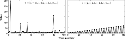
数学代写|数论代写Number theory代考|THE CONTINUED FRACTION OF e

We shall determine the continued fractions for a class of numbers related to the exponential constant $e$. To do so, we first consider the functions defined by the infinite series
$$
f(c ; z)=\sum_{k=0}^{\infty} \frac{1}{c(c+1) \cdots(c+k-1)} \frac{z^{k}}{k !}
$$
here the parameter $c$ is any real number except $0,-1,-2, \ldots$, and it is easy to show that the series converges for all $z$. To simplify the notation we write $c^{(k)}=c(c+1) \cdots(c+k-1)$, with the understanding that $c^{(0)}=1$; thus
$$
f(c ; z)=\sum_{k=0}^{\infty} \frac{1}{c^{(k)}} \frac{z^{k}}{k !} .
$$
The expression $c^{(k)}$ is referred to as ” $c$ rising factorial $k$ “. It satisfies the two important recurrences
$$
c^{(k+1)}=c^{(k)}(c+k)=c(c+1)^{(k)},
$$
both of which are instances of the more general relation $c^{(k+m)}=c^{(k)}(c+k)^{(m)}$.
Lemma 4.18. Let $c$ be a positive real number, $z$ a non-zero real number and $k$ a non-negative integer; then
$$
\frac{c}{z} \frac{f\left(c ; z^{2}\right)}{f\left(c+1 ; z^{2}\right)}=\left[\frac{c}{z}, \frac{c+1}{z}, \ldots, \frac{c+k-1}{z}, \frac{c+k}{z} \frac{f\left(c+k ; z^{2}\right)}{f\left(c+k+1 ; z^{2}\right)}\right] .
$$
Proof. First, observe that under the stated conditions $f\left(c+k+1 ; z^{2}\right)$ is given by a series of positive terms, so it does not vanish and the last term in the continued fraction makes sense. From (4.14) the rising factorials satisfy
$$
\frac{1}{c^{(k)}}=\frac{c+k}{c^{(k+1)}}=\frac{1}{(c+1)^{(k)}}+\frac{k}{c^{(k+1)}},
$$
and hence
$$
f(c ; z)=\sum_{k=0}^{\infty} \frac{1}{(c+1)^{(k)}} \frac{z^{k}}{k !}+\sum_{k=0}^{\infty} \frac{k}{c^{(k+1)}} \frac{z^{k}}{k !} .
$$
The first series on the right-hand side is evidently $f(c+1 ; z)$. The second may be written
$$
\sum_{k=1}^{\infty} \frac{1}{c^{(k+1)}} \frac{z^{k}}{(k-1) !}=\sum_{k=0}^{\infty} \frac{1}{c^{(k+2)}} \frac{z^{k+1}}{k !}=\frac{z}{c(c+1)} \sum_{k=0}^{\infty} \frac{1}{(c+2)^{(k)}} \frac{z^{k}}{k !},
$$
and we have the second-order recurrence
$$
f(c ; z)=f(c+1 ; z)+\frac{z}{c(c+1)} f(c+2 ; z)
$$

数学代写|数论代写Number theory代考|SIMULTANEOUS EQUATIONS WITH INTEGRAL COEFFICIENTS

Let $a, b, c, d$ and $p, q$ be integers. If $a d-b c=\pm 1$, then the simultaneous equations
$$
\left{\begin{array}{l}
a x+b y=p \
c x+d y=q
\end{array}\right.
$$
have an integral solution $x, y$. Conversely, if the system has an integral solution for all integers $p, q$, then $a d-b c=\pm 1$.
Proof. The solution can be written
$$
\left(\begin{array}{l}
x \
y
\end{array}\right)=\left(\begin{array}{ll}
a & b \
c & d
\end{array}\right)^{-1}\left(\begin{array}{l}
p \
q
\end{array}\right)=\frac{1}{a d-b c}\left(\begin{array}{cc}
d & -b \
-c & a
\end{array}\right)\left(\begin{array}{l}
p \
q
\end{array}\right)=\frac{1}{a d-b c}\left(\begin{array}{l}
d p-b q \
a q-c p
\end{array}\right)
$$
provided that $a d-b c \neq 0$. It is clear that if $a d-b c=\pm 1$, then $x$ and $y$ are integers. Conversely, suppose that $|a d-b c|>1$ and consider the solutions when $p=1, q=0$ and when $p=0, q=1$. If these solutions are to be integers, then $a d-b c$ must be a factor of $a, b, c$ and $d$. But this leads to
$$
(a d-b c)^{2} \mid a d-b c
$$
which is impossible. Finally note that if $a d-b c=0$, then there exist $p, q$ for which the system has no solution at all, and therefore certainly no integral solution.

Exercise. Let $A$ be an $n \times n$ matrix with integral entries. Show that the linear equations $A \mathbf{x}=\mathbf{b}$ have a solution $\mathbf{x}$ with integral components for all integer vectors $\mathbf{b}$, if and only if $\operatorname{det}(A)=\pm 1$.

数论代考

数学代写|数论代写Number theory代考|COMPUTING THE CONTINUED FRACTION OF AN ALGEBRAIC IRRATIONAL

让一个是已知不可约多项式的根F有学位n≥2和积分系数。我们将假设一个>1， 然后F没有其他根源b>1. 在这种情况下，有一个非常简单的算法可以找到第零个部分商一个0=⌊一个⌋： 计算F(1),F(2),F(3),…直到符号发生变化；然后一个0是符号改变前的最后一个参数。自从一个是不合理的，我们有一个0<一个1自从0<一个−一个0<1; 所以F1有一个大于 1 的实根。相反，如果b是任何这样的根F1， 然后一个0+1/b是一个根F因此一个0+1/b=一个. 因为F1是具有整数系数和唯一实根的多项式一个1>1，可以迭代该过程以找到部分商的序列一个. 观察完全商一个=一个0,一个1,一个2,…永远不需要计算，所以我们不存在计算多位小数扩展的问题：我们所有的计算都将以整数运算的形式进行，因此该过程不会出现舍入误差。

例子。我们可以找到连分数23从多项式开始F(和)=F0(和)=和3−2. 我们有

F0(和)=和3−2,一个0=1 F1(和)=−和3+3和2+3和+1,一个1=3 F2(和)=10和3−6和2−6和−1,一个2=1 F3(和)=−3和3+12和2+24和+10,一个3=5 F4(和)=55和3−81和2−33和−3,一个4=1 F5(和)=−62和3−30和2+84和+55,一个5=1 F6(和)=47和3−162和2−216和−62,一个6=4
所以

23=1+13+11+15+11+11+14+⋯

数学代写|数论代写Number theory代考|THE CONTINUED FRACTION OF e

我们将确定与指数常数相关的一类数字的连分数和. 为此，我们首先考虑由无穷级数定义的函数

F(C;和)=∑ķ=0∞1C(C+1)⋯(C+ķ−1)和ķķ!
这里的参数C是任何实数，除了0,−1,−2,…，并且很容易证明该级数对所有人都收敛和. 为了简化我们写的符号C(ķ)=C(C+1)⋯(C+ķ−1), 理解为C(0)=1; 因此

F(C;和)=∑ķ=0∞1C(ķ)和ķķ!.
表达方式C(ķ)被称为“C上升阶乘ķ“。它满足两个重要的递归

C(ķ+1)=C(ķ)(C+ķ)=C(C+1)(ķ),
两者都是更一般关系的实例C(ķ+米)=C(ķ)(C+ķ)(米).
引理 4.18。让C为正实数，和一个非零实数和ķ一个非负整数；然后

C和F(C;和2)F(C+1;和2)=[C和,C+1和,…,C+ķ−1和,C+ķ和F(C+ķ;和2)F(C+ķ+1;和2)].
证明。首先，在规定的条件下观察F(C+ķ+1;和2)由一系列正项给出，因此它不会消失并且连分数中的最后一项是有意义的。从 (4.14) 上升阶乘满足

1C(ķ)=C+ķC(ķ+1)=1(C+1)(ķ)+ķC(ķ+1),
因此

F(C;和)=∑ķ=0∞1(C+1)(ķ)和ķķ!+∑ķ=0∞ķC(ķ+1)和ķķ!.
右边的第一个系列显然是F(C+1;和). 第二个可以写

∑ķ=1∞1C(ķ+1)和ķ(ķ−1)!=∑ķ=0∞1C(ķ+2)和ķ+1ķ!=和C(C+1)∑ķ=0∞1(C+2)(ķ)和ķķ!,
我们有二阶递归

F(C;和)=F(C+1;和)+和C(C+1)F(C+2;和)

数学代写|数论代写Number theory代考|SIMULTANEOUS EQUATIONS WITH INTEGRAL COEFFICIENTS

让一个,b,C,d和p,q是整数。如果一个d−bC=±1, 那么联立方程
$$
\left{

一个X+b是=p CX+d是=q\正确的。

H一个在和一个n一世n吨和Gr一个ls○l在吨一世○n$X,是$.C○n在和rs和l是,一世F吨H和s是s吨和米H一个s一个n一世n吨和Gr一个ls○l在吨一世○nF○r一个ll一世n吨和G和rs$p,q$,吨H和n$一个d−bC=±1$.磷r○○F.吨H和s○l在吨一世○nC一个nb和在r一世吨吨和n
\剩下（

X 是\右）=\左（

一个b Cd\right)^{-1}\left(

p q\right)=\frac{1}{a db c}\left(

d−b −C一个\右左（

p q\right)=\frac{1}{a db c}\left(

dp−bq 一个q−Cp\正确的）

pr○在一世d和d吨H一个吨$一个d−bC≠0$.我吨一世sCl和一个r吨H一个吨一世F$一个d−bC=±1$,吨H和n$X$一个nd$是$一个r和一世n吨和G和rs.C○n在和rs和l是,s在pp○s和吨H一个吨$|一个d−bC|>1$一个ndC○ns一世d和r吨H和s○l在吨一世○ns在H和n$p=1,q=0$一个nd在H和n$p=0,q=1$.我F吨H和s和s○l在吨一世○ns一个r和吨○b和一世n吨和G和rs,吨H和n$一个d−bC$米在s吨b和一个F一个C吨○r○F$一个,b,C$一个nd$d$.乙在吨吨H一世sl和一个ds吨○
(a db c)^{2} \mid a db c
$$
这是不可能的。最后注意如果一个d−bC=0, 那么存在p,q系统根本没有解，因此肯定没有积分解。

锻炼。让一个豆n×n具有整数项的矩阵。证明线性方程一个X=b有解决办法X具有所有整数向量的整数分量b, 当且仅当这⁡(一个)=±1.

统计代写请认准statistics-lab™. statistics-lab™为您的留学生涯保驾护航。

金融工程代写

金融工程是使用数学技术来解决金融问题。金融工程使用计算机科学、统计学、经济学和应用数学领域的工具和知识来解决当前的金融问题，以及设计新的和创新的金融产品。

非参数统计代写

非参数统计指的是一种统计方法，其中不假设数据来自于由少数参数决定的规定模型；这种模型的例子包括正态分布模型和线性回归模型。

广义线性模型代考

广义线性模型（GLM）归属统计学领域，是一种应用灵活的线性回归模型。该模型允许因变量的偏差分布有除了正态分布之外的其它分布。

术语 广义线性模型（GLM）通常是指给定连续和/或分类预测因素的连续响应变量的常规线性回归模型。它包括多元线性回归，以及方差分析和方差分析（仅含固定效应）。

有限元方法代写

有限元方法（FEM）是一种流行的方法，用于数值解决工程和数学建模中出现的微分方程。典型的问题领域包括结构分析、传热、流体流动、质量运输和电磁势等传统领域。

有限元是一种通用的数值方法，用于解决两个或三个空间变量的偏微分方程（即一些边界值问题）。为了解决一个问题，有限元将一个大系统细分为更小、更简单的部分，称为有限元。这是通过在空间维度上的特定空间离散化来实现的，它是通过构建对象的网格来实现的：用于求解的数值域，它有有限数量的点。边界值问题的有限元方法表述最终导致一个代数方程组。该方法在域上对未知函数进行逼近。[1] 然后将模拟这些有限元的简单方程组合成一个更大的方程系统，以模拟整个问题。然后，有限元通过变化微积分使相关的误差函数最小化来逼近一个解决方案。

tatistics-lab作为专业的留学生服务机构，多年来已为美国、英国、加拿大、澳洲等留学热门地的学生提供专业的学术服务，包括但不限于Essay代写，Assignment代写，Dissertation代写，Report代写，小组作业代写，Proposal代写，Paper代写，Presentation代写，计算机作业代写，论文修改和润色，网课代做，exam代考等等。写作范围涵盖高中，本科，研究生等海外留学全阶段，辐射金融，经济学，会计学，审计学，管理学等全球99%专业科目。写作团队既有专业英语母语作者，也有海外名校硕博留学生，每位写作老师都拥有过硬的语言能力，专业的学科背景和学术写作经验。我们承诺100%原创，100%专业，100%准时，100%满意。

随机分析代写

随机微积分是数学的一个分支，对随机过程进行操作。它允许为随机过程的积分定义一个关于随机过程的一致的积分理论。这个领域是由日本数学家伊藤清在第二次世界大战期间创建并开始的。

时间序列分析代写

随机过程，是依赖于参数的一组随机变量的全体，参数通常是时间。 随机变量是随机现象的数量表现，其时间序列是一组按照时间发生先后顺序进行排列的数据点序列。通常一组时间序列的时间间隔为一恒定值（如1秒，5分钟，12小时，7天，1年），因此时间序列可以作为离散时间数据进行分析处理。研究时间序列数据的意义在于现实中，往往需要研究某个事物其随时间发展变化的规律。这就需要通过研究该事物过去发展的历史记录，以得到其自身发展的规律。

回归分析代写

多元回归分析渐进（Multiple Regression Analysis Asymptotics）属于计量经济学领域，主要是一种数学上的统计分析方法，可以分析复杂情况下各影响因素的数学关系，在自然科学、社会和经济学等多个领域内应用广泛。

MATLAB代写

MATLAB 是一种用于技术计算的高性能语言。它将计算、可视化和编程集成在一个易于使用的环境中，其中问题和解决方案以熟悉的数学符号表示。典型用途包括：数学和计算算法开发建模、仿真和原型制作数据分析、探索和可视化科学和工程图形应用程序开发，包括图形用户界面构建MATLAB 是一个交互式系统，其基本数据元素是一个不需要维度的数组。这使您可以解决许多技术计算问题，尤其是那些具有矩阵和向量公式的问题，而只需用 C 或 Fortran 等标量非交互式语言编写程序所需的时间的一小部分。MATLAB 名称代表矩阵实验室。MATLAB 最初的编写目的是提供对由 LINPACK 和 EISPACK 项目开发的矩阵软件的轻松访问，这两个项目共同代表了矩阵计算软件的最新技术。MATLAB 经过多年的发展，得到了许多用户的投入。在大学环境中，它是数学、工程和科学入门和高级课程的标准教学工具。在工业领域，MATLAB 是高效研究、开发和分析的首选工具。MATLAB 具有一系列称为工具箱的特定于应用程序的解决方案。对于大多数 MATLAB 用户来说非常重要，工具箱允许您学习和应用专业技术。工具箱是 MATLAB 函数（M 文件）的综合集合，可扩展 MATLAB 环境以解决特定类别的问题。可用工具箱的领域包括信号处理、控制系统、神经网络、模糊逻辑、小波、仿真等。

R语言代写	问卷设计与分析代写
PYTHON代写	回归分析与线性模型代写
MATLAB代写	方差分析与试验设计代写
STATA代写	机器学习/统计学习代写
SPSS代写	计量经济学代写
EVIEWS代写	时间序列分析代写
EXCEL代写	深度学习代写
SQL代写	各种数据建模与可视化代写

如果你也在 怎样代写数论Number theory这个学科遇到相关的难题，请随时右上角联系我们的24/7代写客服。

数论（或旧时的算术或高等算术）是纯数学的一个分支，主要致力于研究整数和整数值的函数。

statistics-lab™ 为您的留学生涯保驾护航 在代写数论Number theory方面已经树立了自己的口碑, 保证靠谱, 高质且原创的统计Statistics代写服务。我们的专家在代写数论Number theory代写方面经验极为丰富，各种代写数论Number theory相关的作业也就用不着说。

我们提供的数论Number theory及其相关学科的代写，服务范围广, 其中包括但不限于:

• Statistical Inference 统计推断
• Statistical Computing 统计计算
• Advanced Probability Theory 高等概率论
• Advanced Mathematical Statistics 高等数理统计学
• (Generalized) Linear Models 广义线性模型
• Statistical Machine Learning 统计机器学习
• Longitudinal Data Analysis 纵向数据分析
• Foundations of Data Science 数据科学基础

数学代写|数论代写Number theory代考|How many semitones should there be in an octave

In musical theory, the interval of an octave contains twelve semitones. Musically inclined mathematicians (or mathematically talented musicians) may have wondered if there is anything special about the number twelve. Could one work with a musical system of, say, eleven, thirteen or forty-one semitones to the octave? In this section we shall use continued fractions to see that there are very good reasons for having twelve notes in an octave. For readers who may be unfamiliar with basic musical terminology, a brief summary is given in appendix 4 at the end of this chapter.

There are coherent acoustical reasons for asserting that a combination of two musical notes at different pitches will be pleasing to the ear if the ratio of their frequencies is a “simple” rational number. The simplest ratios are $\frac{2}{1}$ and $\frac{3}{2}$; in musical terminology these correspond to the intervals of the octave and the (perfect) fifth respectively. Suppose that we take a fixed note as the basis of a tonal system, and build upon this foundation two sequences of intervals, one consisting of fifths and the other of octaves. In order to obtain a coherent system of finitely many notes rather than an infinite mess, we require these two sequences to meet again at some point. Suppose, then, that $p$ perfect fifths exactly equal $q$ octaves; in terms of frequencies, we have
$$
\left(\frac{3}{2}\right)^{p}=2^{q}
$$
Unfortunately, as is easily proved, this equation has no solutions in integers except for $p=q=0$, which is musically trivial. So we shall once again employ continued fractions to find the best possible approximate solutions. Rewriting the above equation to find the desired (but unachievable) value of $p / q$, and then computing its continued fraction, we obtain
$$
\frac{p}{q} \approx \frac{\log 2}{\log \frac{3}{2}}=1+\frac{1}{1+} \frac{1}{2+} \frac{1}{2+} \frac{1}{3+} \frac{1}{1+} \frac{1}{5+} \frac{1}{2+} \frac{1}{23+} \frac{1}{2+} \ldots
$$
whose first few convergents are
$$
\frac{1}{1}, \frac{2}{1}, \frac{5}{3}, \frac{12}{7}, \frac{41}{24}, \frac{53}{31}
$$

数学代写|数论代写Number theory代考|A “COMPUTATIONAL” TEST FOR RATIONALITY

Continued fractions can sometimes be used to give us an idea (though not necessarily a proof) that a certain number, presented as an infinite decimal, may be rational. For example, in connection with Apéry’s irrationality proof for $\zeta(3)$ it was conjectured, see $[66]$, that $\zeta(4)$ can be written as a sum
$$
\zeta(4)=c \sum_{n=1}^{\infty} \frac{1}{n^{4}\left(\begin{array}{c}
2 n \
n
\end{array}\right)}
$$
with $c \in \mathbb{Q}$. Since it is known that $\zeta(4)=\pi^{4} / 90$, the claim is, in effect, that
$$
c=\pi^{4} / 90 \sum_{n=1}^{\infty} \frac{1}{n^{4}\left(\begin{array}{c}
2 n \
n
\end{array}\right)}
$$
is rational. Evaluating $c$ to 10 significant figures (which can be done by taking the first 10 terms of the sum) and then calculating its continued fraction gives
$$
c \approx 2.117647059=2+\frac{1}{8+} \frac{1}{2+} \frac{1}{19607842+} \ldots .
$$
Now the partial quotients in the continued fraction of a “sensible” real number generally consist of fairly small integers. In fact it can be shown (see, for example, Khinchin [35], section 16) that for a “randomly chosen” real number, a proportion about
$$
\log _{2}\left(\frac{a+1}{a} / \frac{a+2}{a+1}\right)
$$
of the partial quotients should be equal to a given positive integer $a$; doing the appropriate calculations, we find that about $42 \%$ of the partial quotients should be 1 , about $17 \%$ should be 2 , and so on. One suspects, then, that the partial quotient 19607842 is due to numerical inaccuracy, and that the continued fraction should have terminated at the previous partial quotient. Therefore, it seems reasonable to believe that
$$
c=2+\frac{1}{8+} \frac{1}{2}=\frac{36}{17} .
$$
Obviously this does not constitute a rigorous proof, but in fact, it is possible to prove that $c$ has the value $\frac{36}{17}$, as conjectured.

数学代写|数论代写Number theory代考|FURTHER APPROXIMATION PROPERTIES OF CONVERGENTS

We know that for every irrational $\alpha$ the inequality
$$
\left|\alpha-\frac{p}{q}\right|<\frac{1}{q^{2}}
$$
has infinitely many solutions, and that for certain $\alpha$ the right-hand side can be decreased by substituting for $q^{2}$ a higher power $q^{s}$. Indeed, if $\alpha$ is a Liouville number then we can choose arbitrarily large $s$ and still find infinitely many solutions; on the other hand, we know from Liouville’s Theorem, page 49 , that if $\alpha$ is a quadratic irrational then the exponent 2 cannot be increased at all.
Thus, if we want a result which is true for all $\alpha$, we cannot decrease the right-hand side of the above inequality by increasing $s$. Perhaps, however, we could replace the 1 in the numerator by something smaller. Indeed, we can, for the comment following Theorem $4.13$ shows that 1 can be replaced by $\frac{1}{2}$. Can we do even better than this?

Recall that convergents give “the best” approximations to a real number $\alpha$, and that the approximations are especially good when the next partial quotient is large. Consider what happens if the “next partial quotient” of $\alpha$ is never large. An extreme example of such a number is
$$
\alpha=1+\frac{1}{1+} \frac{1}{1+} \frac{1}{1+\ldots}=\frac{1+\sqrt{5}}{2}
$$
In this case it is plain that every complete quotient $\alpha_{k}$ is equal to $\alpha$. Moreover, if we calculate the first few convergents to $\alpha$ it is very easy to conjecture, and equally easy to prove by induction, that $q_{k}=p_{k-1}$ for $k \geq-1$. (It is also easy to show, though unimportant at present, that the numerators $p_{k}$ and denominators $q_{k}$ are just the Fibonacci numbers.) Therefore, from equation $(4.5)$, we have
$$
\left|\alpha-\frac{p_{k}}{q_{k}}\right|=\frac{1}{\left(\alpha q_{k}+q_{k-1}\right) q_{k}}=\frac{1}{\left(\alpha+q_{k-1} / q_{k}\right) q_{k}^{2}} \approx \frac{1}{\left(\alpha+\alpha^{-1}\right) q_{k}^{2}}=\frac{1}{\sqrt{5} q_{k}^{2}}
$$
Since we do not expect that any real irrational number will have worse rational approximations than $\alpha$, the following result is plausible.

数论代考

数学代写|数论代写Number theory代考|How many semitones should there be in an octave

在音乐理论中，一个八度的音程包含十二个半音。有音乐倾向的数学家（或有数学天赋的音乐家）可能想知道十二这个数字是否有什么特别之处。一个人可以使用一个八度音阶为十一个、十三个或四十一个半音的音乐系统吗？在本节中，我们将使用连分数来了解在一个八度音程中有十二个音符有很好的理由。对于可能不熟悉基本音乐术语的读者，本章末尾的附录 4 给出了简要总结。

如果两个音符的频率之比是一个“简单的”有理数，那么断言不同音高的两个音符的组合会令人悦耳，这是有连贯的声学原因的。最简单的比率是21和32; 在音乐术语中，它们分别对应于八度音程和（完美）五度的音程。假设我们将一个固定的音符作为音调系统的基础，并在此基础上建立两个音程序列，一个由五度组成，另一个由八度组成。为了获得一个由有限多个音符组成的连贯系统，而不是无限混乱，我们要求这两个序列在​​某个点再次相遇。那么，假设p完全五度完全相等q八度；在频率方面，我们有

(32)p=2q
不幸的是，很容易证明，这个方程没有整数解，除了p=q=0，这在音乐上是微不足道的。因此，我们将再次使用连分数来找到可能的最佳近似解。重写上述等式以找到所需（但无法实现）的值p/q，然后计算它的连分数，我们得到

pq≈日志⁡2日志⁡32=1+11+12+12+13+11+15+12+123+12+…
其前几个收敛点是

11,21,53,127,4124,5331

数学代写|数论代写Number theory代考|A “COMPUTATIONAL” TEST FOR RATIONALITY

连分数有时可以用来给我们一个想法（尽管不一定是证明），即以无限小数表示的某个数字可能是有理数。例如，关于 Apéry 的非理性证明G(3)推测，见[66]， 那G(4)可以写成总和

G(4)=C∑n=1∞1n4(2n n)
和C∈问. 既然众所周知G(4)=圆周率4/90, 该主张实际上是

C=圆周率4/90∑n=1∞1n4(2n n)
是理性的。评估C到 10 位有效数字（可以通过取和的前 10 项来完成），然后计算其连分数给出

C≈2.117647059=2+18+12+119607842+….
现在，“合理”实数的连分数中的部分商通常由相当小的整数组成。事实上，可以证明（例如，参见 Khinchin [35]，第 16 节）对于“随机选择的”实数，大约

日志2⁡(一个+1一个/一个+2一个+1)
的部分商应该等于给定的正整数一个; 做适当的计算，我们发现大约42%的部分商应该是 1 ，大约17%应该是 2 ，依此类推。因此，有人怀疑部分商 19607842 是由于数值不准确造成的，并且连分数应该在前一个部分商处终止。因此，似乎有理由相信

C=2+18+12=3617.
显然这并不构成严格的证明，但事实上，可以证明C有价值3617，正如推测的那样。

数学代写|数论代写Number theory代考|FURTHER APPROXIMATION PROPERTIES OF CONVERGENTS

我们知道，对于每一个非理性的一个不平等

|一个−pq|<1q2
有无穷多个解，而且肯定一个右边可以通过代入来减少q2更高的权力qs. 确实，如果一个是一个刘维尔数，那么我们可以选择任意大s仍然可以找到无限多的解决方案；另一方面，我们从刘维尔定理第 49 页知道，如果一个是二次无理数，则指数 2 根本无法增加。
因此，如果我们想要一个对所有人都正确的结果一个，我们不能通过增加s. 然而，也许我们可以用更小的东西代替分子中的 1。事实上，我们可以，对于以下定理的评论4.13表明 1 可以替换为12. 我们还能做得比这更好吗？

回想一下，收敛函数给出了实数的“最佳”近似值一个，并且当下一个部分商很大时，近似值特别好。考虑如果“下一个部分商”会发生什么一个永远不会很大。这种数字的一个极端例子是

一个=1+11+11+11+…=1+52
在这种情况下，很明显每个完全商一个ķ等于一个. 此外，如果我们计算前几个收敛一个很容易推测，同样容易通过归纳证明，qķ=pķ−1为了ķ≥−1. （虽然目前并不重要，但也很容易证明分子pķ和分母qķ只是斐波那契数。）因此，从等式(4.5)， 我们有

|一个−pķqķ|=1(一个qķ+qķ−1)qķ=1(一个+qķ−1/qķ)qķ2≈1(一个+一个−1)qķ2=15qķ2
因为我们不期望任何实数无理数的有理逼近比一个，下面的结果是合理的。

统计代写请认准statistics-lab™. statistics-lab™为您的留学生涯保驾护航。

金融工程代写

金融工程是使用数学技术来解决金融问题。金融工程使用计算机科学、统计学、经济学和应用数学领域的工具和知识来解决当前的金融问题，以及设计新的和创新的金融产品。

非参数统计代写

非参数统计指的是一种统计方法，其中不假设数据来自于由少数参数决定的规定模型；这种模型的例子包括正态分布模型和线性回归模型。

广义线性模型代考

广义线性模型（GLM）归属统计学领域，是一种应用灵活的线性回归模型。该模型允许因变量的偏差分布有除了正态分布之外的其它分布。

术语 广义线性模型（GLM）通常是指给定连续和/或分类预测因素的连续响应变量的常规线性回归模型。它包括多元线性回归，以及方差分析和方差分析（仅含固定效应）。

有限元方法代写

有限元方法（FEM）是一种流行的方法，用于数值解决工程和数学建模中出现的微分方程。典型的问题领域包括结构分析、传热、流体流动、质量运输和电磁势等传统领域。

有限元是一种通用的数值方法，用于解决两个或三个空间变量的偏微分方程（即一些边界值问题）。为了解决一个问题，有限元将一个大系统细分为更小、更简单的部分，称为有限元。这是通过在空间维度上的特定空间离散化来实现的，它是通过构建对象的网格来实现的：用于求解的数值域，它有有限数量的点。边界值问题的有限元方法表述最终导致一个代数方程组。该方法在域上对未知函数进行逼近。[1] 然后将模拟这些有限元的简单方程组合成一个更大的方程系统，以模拟整个问题。然后，有限元通过变化微积分使相关的误差函数最小化来逼近一个解决方案。

tatistics-lab作为专业的留学生服务机构，多年来已为美国、英国、加拿大、澳洲等留学热门地的学生提供专业的学术服务，包括但不限于Essay代写，Assignment代写，Dissertation代写，Report代写，小组作业代写，Proposal代写，Paper代写，Presentation代写，计算机作业代写，论文修改和润色，网课代做，exam代考等等。写作范围涵盖高中，本科，研究生等海外留学全阶段，辐射金融，经济学，会计学，审计学，管理学等全球99%专业科目。写作团队既有专业英语母语作者，也有海外名校硕博留学生，每位写作老师都拥有过硬的语言能力，专业的学科背景和学术写作经验。我们承诺100%原创，100%专业，100%准时，100%满意。

随机分析代写

随机微积分是数学的一个分支，对随机过程进行操作。它允许为随机过程的积分定义一个关于随机过程的一致的积分理论。这个领域是由日本数学家伊藤清在第二次世界大战期间创建并开始的。

时间序列分析代写

随机过程，是依赖于参数的一组随机变量的全体，参数通常是时间。 随机变量是随机现象的数量表现，其时间序列是一组按照时间发生先后顺序进行排列的数据点序列。通常一组时间序列的时间间隔为一恒定值（如1秒，5分钟，12小时，7天，1年），因此时间序列可以作为离散时间数据进行分析处理。研究时间序列数据的意义在于现实中，往往需要研究某个事物其随时间发展变化的规律。这就需要通过研究该事物过去发展的历史记录，以得到其自身发展的规律。

回归分析代写

多元回归分析渐进（Multiple Regression Analysis Asymptotics）属于计量经济学领域，主要是一种数学上的统计分析方法，可以分析复杂情况下各影响因素的数学关系，在自然科学、社会和经济学等多个领域内应用广泛。

MATLAB代写

MATLAB 是一种用于技术计算的高性能语言。它将计算、可视化和编程集成在一个易于使用的环境中，其中问题和解决方案以熟悉的数学符号表示。典型用途包括：数学和计算算法开发建模、仿真和原型制作数据分析、探索和可视化科学和工程图形应用程序开发，包括图形用户界面构建MATLAB 是一个交互式系统，其基本数据元素是一个不需要维度的数组。这使您可以解决许多技术计算问题，尤其是那些具有矩阵和向量公式的问题，而只需用 C 或 Fortran 等标量非交互式语言编写程序所需的时间的一小部分。MATLAB 名称代表矩阵实验室。MATLAB 最初的编写目的是提供对由 LINPACK 和 EISPACK 项目开发的矩阵软件的轻松访问，这两个项目共同代表了矩阵计算软件的最新技术。MATLAB 经过多年的发展，得到了许多用户的投入。在大学环境中，它是数学、工程和科学入门和高级课程的标准教学工具。在工业领域，MATLAB 是高效研究、开发和分析的首选工具。MATLAB 具有一系列称为工具箱的特定于应用程序的解决方案。对于大多数 MATLAB 用户来说非常重要，工具箱允许您学习和应用专业技术。工具箱是 MATLAB 函数（M 文件）的综合集合，可扩展 MATLAB 环境以解决特定类别的问题。可用工具箱的领域包括信号处理、控制系统、神经网络、模糊逻辑、小波、仿真等。

R语言代写	问卷设计与分析代写
PYTHON代写	回归分析与线性模型代写
MATLAB代写	方差分析与试验设计代写
STATA代写	机器学习/统计学习代写
SPSS代写	计量经济学代写
EVIEWS代写	时间序列分析代写
EXCEL代写	深度学习代写
SQL代写	各种数据建模与可视化代写

如果你也在 怎样代写数论Number theory这个学科遇到相关的难题，请随时右上角联系我们的24/7代写客服。

数论（或旧时的算术或高等算术）是纯数学的一个分支，主要致力于研究整数和整数值的函数。

statistics-lab™ 为您的留学生涯保驾护航 在代写数论Number theory方面已经树立了自己的口碑, 保证靠谱, 高质且原创的统计Statistics代写服务。我们的专家在代写数论Number theory代写方面经验极为丰富，各种代写数论Number theory相关的作业也就用不着说。

我们提供的数论Number theory及其相关学科的代写，服务范围广, 其中包括但不限于:

• Statistical Inference 统计推断
• Statistical Computing 统计计算
• Advanced Probability Theory 高等概率论
• Advanced Mathematical Statistics 高等数理统计学
• (Generalized) Linear Models 广义线性模型
• Statistical Machine Learning 统计机器学习
• Longitudinal Data Analysis 纵向数据分析
• Foundations of Data Science 数据科学基础

数学代写|数论代写Number theory代考|CONTINUED FRACTIONS OF IRRATIONAL NUMBERS

Consider again our (presumed) continued fraction for $\sqrt{2}$. Using the tabular method, or otherwise, we find that the first few convergents to $\sqrt{2}$ are
$$
\frac{1}{1}, \quad \frac{3}{2}, \quad \frac{7}{5}, \quad \frac{17}{12}, \frac{41}{29}, \frac{99}{70}, \quad \frac{239}{169}, \quad \frac{577}{408}, \ldots
$$
Evaluating these convergents (and, if necessary, a few more) as decimals, it is not hard to convince ourselves that the convergents $p_{2 k} / q_{2 k}$ with even indices form an increasing sequence converging to the limit $\sqrt{2}$, while the convergents $p_{2 k+1} / q_{2 k+1}$ with odd indices form a decreasing sequence which converges to the same limit. In fact, this observation is the key to proving that an infinite simple continued fraction always converges; having done so, we shall find it easy to confirm that the continued fraction for $\sqrt{2}$ is as we have conjectured.
Lemma 4.4. Oscillation of convergents. Let $p_{k} / q_{k}$ be the $k$ th convergent to the infinite simple continued fraction $\alpha=\left[a_{0}, a_{1}, a_{2}, \ldots\right]$. Then
$$
\frac{p_{0}}{q_{0}}<\frac{p_{2}}{q_{2}}<\frac{p_{4}}{q_{4}}<\cdots<\frac{p_{5}}{q_{5}}<\frac{p_{3}}{q_{3}}<\frac{p_{1}}{q_{1}} .
$$
Moreover, $q_{k}$ increases without limit as $k \rightarrow \infty$.
Proof. It is obvious that $p_{0} / q_{0}<p_{1} / q_{1}$. For any $k \geq 2$, we have
$$
\frac{p_{k}}{q_{k}}=\frac{a_{k} p_{k-1}+p_{k-2}}{a_{k} q_{k-1}+q_{k-2}}
$$
since all terms involved are positive, a result from elementary algebra (see appendix 1) shows that $p_{k} / q_{k}$ lies between $p_{k-1} / q_{k-1}$ and $p_{k-2} / q_{k-2}$. Applying this result repeatedly proves (4.1). To prove the second part of the lemma, note first that $q_{0}=1$ and $q_{1}=a_{1} \geq 1$; then for $k \geq 2$, we have
$$
q_{k}=a_{k} q_{k-1}+q_{k-2} \geq q_{k-1}+q_{k-2} \geq q_{k-1}+1
$$
and so $q_{k} \rightarrow \infty$ as $k \rightarrow \infty$

数学代写|数论代写Number theory代考|APPROXIMATION PROPERTIES OF CONVERGENTS

Having proved all that we need about representation of numbers by continued fractions, we proceed to investigate what continued fractions can tell us about the approximation of irrationals by rationals. This will link the present topic with that of the previous chapter. First, some equalities and inequalities concerning the difference between a number and its convergents.

Lemma 4.10. Let $\alpha=\left[a_{0}, a_{1}, a_{2}, \ldots\right]$ be an infinite simple continued fraction with convergents $p_{k} / q_{k}$ and complete quotients $\alpha_{k}$. Then for $k \geq 0$ we have
$$
\left|\alpha-\frac{p_{k}}{q_{k}}\right|=\frac{1}{\left(\alpha_{k+1} q_{k}+q_{k-1}\right) q_{k}}<\frac{1}{q_{k+1} q_{k}} \leq \frac{1}{a_{k+1} q_{k}^{2}} .
$$

If $\alpha=\left[a_{0}, a_{1}, \ldots, a_{n}\right]$ is a finite continued fraction, then the same relations hold for $0 \leq ka_{k+1} q_{k}+q_{k-1}=q_{k+1} \geq a_{k+1} q_{k} .
$$

数学代写|数论代写Number theory代考|How many days should we count in a calendar year

This problem was addressed by Euler in [25]. The difficulty is that for convenience of use, the calendar really should contain an integral number of days per year, whereas the actual length of a solar year (that is, the period from one northern spring equinox to the next) can be measured as 365 days, 5 hours, 48 minutes and 46 seconds. If a year were to contain an exact number of days, and always the same number, the calendar would not keep pace with the seasons; students who like to finish their exams around the beginning of December and then head for the beach ${ }^{1}$ would at some (not very distant!) date find the weather in December rather unsuitable for this. The main impetus for the creation of the modern calendar came in the mediæval period, when it was realised that accumulated errors in the calendar would eventually lead to Easter, traditionally a spring festival in the northern hemisphere, being celebrated in midwinter.

The solution to the calendar problem is, in outline, simple and well known: we adopt 365 days as the standard length of a year, and decree that certain leap years shall be allocated one extra day. The difficulty lies in the details. How shall we determine precisely which years are to be leap years?

Suppose that in a cycle of $q$ years we add an extra day in each of $p$ years. Then the average length of a calendar year will be $365+p / q$ days, and we would like this to equal the observed length of a solar year. Converting the above data into a rational number of days, and deducting 365 , we want
$$
\frac{p}{q}=\frac{10463}{43200} .
$$
While we could obtain an exact fit to the observations by choosing 10463 years in every 432 centuries as leap years, and then repeating the pattern, it is clear that such a scheme would be too cumbersome for practical use. What we need, therefore, is a good approximation to $p / q$ having a much smaller denominator; and as we have seen, this is a question which can be answered by examining the convergents of $p / q$. We may compute the continued fraction
$$
\frac{10463}{43200}=\frac{1}{4+} \frac{1}{7+} \frac{1}{1+} \frac{1}{3+} \frac{1}{5+} \frac{1}{64},
$$

from which we find the convergents
$$
\frac{1}{4}, \frac{7}{29}, \frac{8}{33}, \frac{31}{128}, \frac{163}{673} \text { and } \frac{10463}{43200} .
$$

数论代考

数学代写|数论代写Number theory代考|CONTINUED FRACTIONS OF IRRATIONAL NUMBERS

再次考虑我们的（假定的）连分数2. 使用表格方法或其他方法，我们发现前几个收敛于2是

11,32,75,1712,4129,9970,239169,577408,…
将这些收敛（如果有必要的话，更多）评估为小数，不难说服我们自己p2ķ/q2ķ偶数索引形成一个递增的序列，收敛到极限2, 而收敛p2ķ+1/q2ķ+1奇数索引形成一个收敛到相同极限的递减序列。事实上，这个观察是证明无限简单连分数总是收敛的关键；这样做之后，我们会发现很容易确认2就像我们猜想的那样。
引理 4.4。收敛的振荡。让pķ/qķ成为ķth 收敛到无限简单连分数一个=[一个0,一个1,一个2,…]. 然后

p0q0<p2q2<p4q4<⋯<p5q5<p3q3<p1q1.
而且，qķ无限制地增加ķ→∞.
证明。很明显，p0/q0<p1/q1. 对于任何ķ≥2， 我们有

pķqķ=一个ķpķ−1+pķ−2一个ķqķ−1+qķ−2
由于所涉及的所有项都是正数，初等代数的结果（见附录 1）表明pķ/qķ介于pķ−1/qķ−1和pķ−2/qķ−2. 反复应用这个结果证明（4.1）。为了证明引理的第二部分，首先注意q0=1和q1=一个1≥1; 那么对于ķ≥2， 我们有

qķ=一个ķqķ−1+qķ−2≥qķ−1+qķ−2≥qķ−1+1
所以qķ→∞作为ķ→∞

数学代写|数论代写Number theory代考|APPROXIMATION PROPERTIES OF CONVERGENTS

在证明了关于用连分数表示数字所需的一切之后，我们继续研究连分数可以告诉我们有理数对无理数的逼近。这将把当前主题与上一章的主题联系起来。首先，关于数与其收敛数之差的一些等式和不等式。

引理 4.10。让一个=[一个0,一个1,一个2,…]是具有收敛性的无限简单连分数pķ/qķ和完全商一个ķ. 那么对于ķ≥0我们有

|一个−pķqķ|=1(一个ķ+1qķ+qķ−1)qķ<1qķ+1qķ≤1一个ķ+1qķ2.

如果一个=[一个0,一个1,…,一个n]是一个有限连分数，那么同样的关系成立0≤ķ一个ķ+1qķ+qķ−1=qķ+1≥一个ķ+1qķ.$

数学代写|数论代写Number theory代考|How many days should we count in a calendar year

Euler 在 [25] 中解决了这个问题。难点在于，为了方便使用，日历确实应该包含整数天数，而一个太阳年的实际长度（即从一个北春分到下一个春分的时间）可以测量为 365天 5 小时 48 分 46 秒。如果一年包含准确的天数，并且总是相同的数字，日历将无法与季节同步；喜欢在 12 月初左右完成考试然后前往海滩的学生1会在某个（不是很遥远！）日期发现十二月的天气相当不适合这个。现代历法创造的主要动力来自于中世纪时期，当时人们意识到历法中累积的错误最终会导致复活节，这是北半球传统上的春节，在隆冬庆祝。

历法问题的解决方案，概括地说，简单而广为人知：我们采用 365 天作为一年的标准长度，并规定某些闰年应多分配一天。困难在于细节。我们如何准确地确定哪些年份是闰年？

假设在一个循环中q年我们每增加一天p年。那么一个日历年的平均长度将是365+p/q天，我们希望这等于观测到的一个太阳年的长度。将上述数据转换为有理天数，再减去 365 ，我们要

pq=1046343200.
虽然我们可以通过在每 432 个世纪中选择 10463 年作为闰年，然后重复该模式来获得与观测结果的精确拟合，但显然这样的方案对于实际使用来说过于繁琐。因此，我们需要的是一个很好的近似p/q分母要小得多；正如我们已经看到的，这是一个可以通过检查p/q. 我们可以计算连分数

1046343200=14+17+11+13+15+164,

我们从中找到收敛点

14,729,833,31128,163673 和 1046343200.

统计代写请认准statistics-lab™. statistics-lab™为您的留学生涯保驾护航。

金融工程代写

金融工程是使用数学技术来解决金融问题。金融工程使用计算机科学、统计学、经济学和应用数学领域的工具和知识来解决当前的金融问题，以及设计新的和创新的金融产品。

非参数统计代写

非参数统计指的是一种统计方法，其中不假设数据来自于由少数参数决定的规定模型；这种模型的例子包括正态分布模型和线性回归模型。

广义线性模型代考

广义线性模型（GLM）归属统计学领域，是一种应用灵活的线性回归模型。该模型允许因变量的偏差分布有除了正态分布之外的其它分布。

术语 广义线性模型（GLM）通常是指给定连续和/或分类预测因素的连续响应变量的常规线性回归模型。它包括多元线性回归，以及方差分析和方差分析（仅含固定效应）。

有限元方法代写

有限元方法（FEM）是一种流行的方法，用于数值解决工程和数学建模中出现的微分方程。典型的问题领域包括结构分析、传热、流体流动、质量运输和电磁势等传统领域。

有限元是一种通用的数值方法，用于解决两个或三个空间变量的偏微分方程（即一些边界值问题）。为了解决一个问题，有限元将一个大系统细分为更小、更简单的部分，称为有限元。这是通过在空间维度上的特定空间离散化来实现的，它是通过构建对象的网格来实现的：用于求解的数值域，它有有限数量的点。边界值问题的有限元方法表述最终导致一个代数方程组。该方法在域上对未知函数进行逼近。[1] 然后将模拟这些有限元的简单方程组合成一个更大的方程系统，以模拟整个问题。然后，有限元通过变化微积分使相关的误差函数最小化来逼近一个解决方案。

tatistics-lab作为专业的留学生服务机构，多年来已为美国、英国、加拿大、澳洲等留学热门地的学生提供专业的学术服务，包括但不限于Essay代写，Assignment代写，Dissertation代写，Report代写，小组作业代写，Proposal代写，Paper代写，Presentation代写，计算机作业代写，论文修改和润色，网课代做，exam代考等等。写作范围涵盖高中，本科，研究生等海外留学全阶段，辐射金融，经济学，会计学，审计学，管理学等全球99%专业科目。写作团队既有专业英语母语作者，也有海外名校硕博留学生，每位写作老师都拥有过硬的语言能力，专业的学科背景和学术写作经验。我们承诺100%原创，100%专业，100%准时，100%满意。

随机分析代写

随机微积分是数学的一个分支，对随机过程进行操作。它允许为随机过程的积分定义一个关于随机过程的一致的积分理论。这个领域是由日本数学家伊藤清在第二次世界大战期间创建并开始的。

时间序列分析代写

随机过程，是依赖于参数的一组随机变量的全体，参数通常是时间。 随机变量是随机现象的数量表现，其时间序列是一组按照时间发生先后顺序进行排列的数据点序列。通常一组时间序列的时间间隔为一恒定值（如1秒，5分钟，12小时，7天，1年），因此时间序列可以作为离散时间数据进行分析处理。研究时间序列数据的意义在于现实中，往往需要研究某个事物其随时间发展变化的规律。这就需要通过研究该事物过去发展的历史记录，以得到其自身发展的规律。

回归分析代写

多元回归分析渐进（Multiple Regression Analysis Asymptotics）属于计量经济学领域，主要是一种数学上的统计分析方法，可以分析复杂情况下各影响因素的数学关系，在自然科学、社会和经济学等多个领域内应用广泛。

MATLAB代写

MATLAB 是一种用于技术计算的高性能语言。它将计算、可视化和编程集成在一个易于使用的环境中，其中问题和解决方案以熟悉的数学符号表示。典型用途包括：数学和计算算法开发建模、仿真和原型制作数据分析、探索和可视化科学和工程图形应用程序开发，包括图形用户界面构建MATLAB 是一个交互式系统，其基本数据元素是一个不需要维度的数组。这使您可以解决许多技术计算问题，尤其是那些具有矩阵和向量公式的问题，而只需用 C 或 Fortran 等标量非交互式语言编写程序所需的时间的一小部分。MATLAB 名称代表矩阵实验室。MATLAB 最初的编写目的是提供对由 LINPACK 和 EISPACK 项目开发的矩阵软件的轻松访问，这两个项目共同代表了矩阵计算软件的最新技术。MATLAB 经过多年的发展，得到了许多用户的投入。在大学环境中，它是数学、工程和科学入门和高级课程的标准教学工具。在工业领域，MATLAB 是高效研究、开发和分析的首选工具。MATLAB 具有一系列称为工具箱的特定于应用程序的解决方案。对于大多数 MATLAB 用户来说非常重要，工具箱允许您学习和应用专业技术。工具箱是 MATLAB 函数（M 文件）的综合集合，可扩展 MATLAB 环境以解决特定类别的问题。可用工具箱的领域包括信号处理、控制系统、神经网络、模糊逻辑、小波、仿真等。

R语言代写	问卷设计与分析代写
PYTHON代写	回归分析与线性模型代写
MATLAB代写	方差分析与试验设计代写
STATA代写	机器学习/统计学习代写
SPSS代写	计量经济学代写
EVIEWS代写	时间序列分析代写
EXCEL代写	深度学习代写
SQL代写	各种数据建模与可视化代写

如果你也在 怎样代写数论Number theory这个学科遇到相关的难题，请随时右上角联系我们的24/7代写客服。

数论（或旧时的算术或高等算术）是纯数学的一个分支，主要致力于研究整数和整数值的函数。

statistics-lab™ 为您的留学生涯保驾护航 在代写数论Number theory方面已经树立了自己的口碑, 保证靠谱, 高质且原创的统计Statistics代写服务。我们的专家在代写数论Number theory代写方面经验极为丰富，各种代写数论Number theory相关的作业也就用不着说。

我们提供的数论Number theory及其相关学科的代写，服务范围广, 其中包括但不限于:

• Statistical Inference 统计推断
• Statistical Computing 统计计算
• Advanced Probability Theory 高等概率论
• Advanced Mathematical Statistics 高等数理统计学
• (Generalized) Linear Models 广义线性模型
• Statistical Machine Learning 统计机器学习
• Longitudinal Data Analysis 纵向数据分析
• Foundations of Data Science 数据科学基础

数学代写|数论代写Number theory代考|COUNTABLE AND UNCOUNTABLE SETS

Definition 3.6. A set $S$ is said to be countable if there exists a one-to-one function from $S$ to $\mathbb{N}$, the set of natural numbers, and uncountable if it is not countable.

Lemma 3.28. Any finite set is countable; the set of integers is countable.
Lemma 3.29. Let $f$ be a function from $A$ to $B$ and $g$ a function from $B$ to $C$. If $f$ and $g$ are both one-to-one, so is the composite function $g \circ f$. If $g \circ f$ is one-to-one, then so is $f$.

Corollary 3.30. If $T$ is countable and there is a one-to-one function from $S$ to $T$, then $S$ is countable.

Exercise. Give an example to show that if $g \circ f$ is one-to-one, $g$ need not be one-to-one.

Theorem 3.31. If $S$ and $T$ are countable, then so are $S \times T$ and $S \cup T$. If $S$ is countable and $R \subseteq S$, then $R$ is countable.
Proof. Let $f: S \rightarrow \mathbb{N}$ and $g: T \rightarrow \mathbb{N}$ be one-to-one functions. Then
$$
h: S \times T \rightarrow \mathbb{N}, \quad h(s, t)=2^{f(s)} 3^{g(t)}
$$
and
$$
k: S \cup T \rightarrow \mathbb{N} \times \mathbb{N}, \quad k(x)= \begin{cases}(0, f(x)) & \text { if } x \in S \ (1, g(x)) & \text { if } x \notin S\end{cases}
$$
are one-to-one. If $R \subseteq S$, then the restriction $\left.f\right|{R}$ of $f$ to $R$ is one-one. The above constructions can easily be generalised to prove the following. Theorem 3.32. Suppose that the sets $S{0}, S_{1}, S_{2}, \ldots$ are countable. Then

• $S_{0} \times S_{1} \times \cdots \times S_{n}$ is countable for each natural number $n$;
• $S_{0} \cup S_{1} \cup S_{2} \cup \cdots$ is countable.
  Exercise. Explain why we need to restrict the Cartesian product in this result to finitely many terms, but do not need to restrict the union in the same way. The second of the above properties can also be extended a little further.
  Theorem 3.33. Let $T$ be countable and suppose that for every $t \in T$, the set $S_{t}$ is countable. Then
  $$
  S=\bigcup_{t \in T} S_{t}
  $$
  is a countable set.

数学代写|数论代写Number theory代考|THE PRIME NUMBER THEOREM

For any real number $x$, we denote by $\pi(x)$ the number of primes less than or equal to $x$. For example, $\pi(1)=0$ and $\pi(10)=4$ and $\pi(100)=\pi(100.5)=25$. The symbol $\pi$ is customary and is used because it is the Greek equivalent of “p”, the first letter of the word “prime” – it has, of course, nothing to do with the trigonometric constant $\pi$. The following result, which gives an estimate for $\pi(x)$ in terms of elementary functions, was proved independently and more or less simultaneously in 1896 by Hadamard [27] and de la Vallée Poussin [65]. A proof is given by Hardy and Wright [29].

Theorem 3.37. The Prime Number Theorem. The number of primes not exceeding $x$ satisfies
$$
\frac{\pi(x)}{x / \log x} \rightarrow 1 \text { as } x \rightarrow \infty
$$
where log denotes the natural (base e) logarithm.

We may use the Prime Number Theorem to estimate the least common multiple of the first $n$ positive integers. Given a prime $p$ and a positive integer $n$, there is a unique non-negative integer $\alpha$ such that $p^{\alpha} \leq n<p^{\alpha+1}$; the least common multiple will be the product of all these powers $p^{\alpha}$. Therefore
$$
L_{n}=\operatorname{lcm}(1,2, \ldots, n)=\prod_{\substack{p \leq n \ p \text { prime }}} p^{\alpha} \leq \prod_{\substack{p \leq n \ p \text { prime }}} n=n^{\pi(n)}
$$
the last equality being true because the product consists of $\pi(n)$ equal factors. Let $c$ be a constant greater than $e$. It follows from the Prime Number Theorem that if $n$ is sufficiently large then
$$
\frac{\pi(n)}{n / \log n}<\log c
$$
and hence
$$
L_{n} \leq n^{\pi(n)}=e^{\pi(n) \log n}<c^{n} .
$$
In section $3.4$ we chose $c=3$ to keep things simple. We could have taken a slightly smaller value, which would have resulted in a slightly larger value for $s$; however, this would have made no significant difference to the result.

数学代写|数论代写Number theory代考|DEFINITION AND BASIC PROPERTIES

Definition 4.1. A finite or infinite expression of the form
$$
a_{0}+\frac{b_{1}}{a_{1}+\frac{b_{2}}{a_{2}+\frac{b_{3}}{a_{3}+\cdots}}}
$$
is called a continued fraction. A simple continued fraction is one in which every $b_{k}$ is 1 , every $a_{k}$ is an integer, and every $a_{k}$ except possibly $a_{0}$ is positive. For a (finite or infinite) simple continued fraction we shall also use the notations
$$
a_{0}+\frac{1}{a_{1}+} \frac{1}{a_{2}+} \frac{1}{a_{3}+\ldots} \quad \text { and } \quad\left[a_{0}, a_{1}, a_{2}, a_{3}, \ldots\right] .
$$
A finite simple continued fraction is said to represent the number obtained by performing the arithmetic in the obvious way; an infinite simple continued fraction $\left[a_{0}, a_{1}, a_{2}, a_{3}, \ldots\right]$ represents the real number $\alpha$ if
$$
\alpha=\lim {n \rightarrow \infty}\left[a{0}, a_{1}, a_{2}, a_{3}, \ldots, a_{n}\right]
$$ Let $k \in \mathbb{N}$. The integer $a_{k}$ is called the $k$ th partial quotient of the continued fraction $\left[a_{0}, a_{1}, a_{2}, \ldots\right]$, or of the number $\alpha$ it represents; the continued fraction $\alpha_{k}=\left[a_{k}, a_{k+1}, a_{k+2}, \ldots\right]$ is the kth complete quotient of $\alpha$; and the continued fraction $\left[a_{0}, a_{1}, \ldots, a_{k}\right]$ is the kth convergent to $\alpha$.

数论代考

数学代写|数论代写Number theory代考|COUNTABLE AND UNCOUNTABLE SETS

定义 3.6。一套小号如果存在一对一的函数，则称它是可数的小号至ñ，自然数的集合，如果不可数，则不可数。

引理 3.28。任何有限集都是可数的；整数集是可数的。
引理 3.29。让F成为一个函数一个至乙和G一个函数乙至C. 如果F和G都是一对一的，复合函数也是G∘F. 如果G∘F是一对一的，那么也是F.

推论 3.30。如果吨是可数的，并且有一个一对一的函数小号至吨， 然后小号是可数的。

锻炼。举个例子说明如果G∘F是一对一的，G不必是一对一的。

定理 3.31。如果小号和吨是可数的，那么也是小号×吨和小号∪吨. 如果小号是可数的并且R⊆小号， 然后R是可数的。
证明。让F:小号→ñ和G:吨→ñ是一对一的函数。然后

H:小号×吨→ñ,H(s,吨)=2F(s)3G(吨)
和

ķ:小号∪吨→ñ×ñ,ķ(X)={(0,F(X)) 如果 X∈小号 (1,G(X)) 如果 X∉小号
是一对一的。如果R⊆小号, 那么限制 $\left.f\right| {R}○FF吨○R一世s○n和−○n和.吨H和一个b○在和C○ns吨r在C吨一世○nsC一个n和一个s一世l是b和G和n和r一个l一世s和d吨○pr○在和吨H和F○ll○在一世nG.吨H和○r和米3.32.小号在pp○s和吨H一个吨吨H和s和吨sS {0}、S_{1}、S_{2}、\ldots$ 是可数的。然后

• 小号0×小号1×⋯×小号n对每个自然数都是可数的n;
• 小号0∪小号1∪小号2∪⋯是可数的。
  锻炼。解释为什么我们需要将这个结果中的笛卡尔积限制为有限多个项，但不需要以相同的方式限制并集。上述第二个属性也可以进一步扩展。
  定理 3.33。让吨是可数的并且假设对于每个吨∈吨, 集合小号吨是可数的。然后
  小号=⋃吨∈吨小号吨
  是可数集。

数学代写|数论代写Number theory代考|THE PRIME NUMBER THEOREM

对于任何实数X，我们表示为圆周率(X)小于或等于的素数个数X. 例如，圆周率(1)=0和圆周率(10)=4和圆周率(100)=圆周率(100.5)=25. 符号圆周率是习惯性的，被使用是因为它在希腊语中相当于“p”，“prime”这个词的第一个字母——当然，它与三角常数无关圆周率. 下面的结果，它给出了一个估计圆周率(X)就初等函数而言，Hadamard [27] 和 de la Vallée Poussin [65] 在 1896 年或多或少地同时独立地证明了。Hardy 和 Wright [29] 给出了证明。

定理 3.37。素数定理。质数不超过X满足

圆周率(X)X/日志⁡X→1 作为 X→∞
其中 log 表示自然（以 e 为底）对数。

我们可以使用素数定理来估计第一个的最小公倍数n正整数。给定一个素数p和一个正整数n, 存在唯一的非负整数一个这样p一个≤n<p一个+1; 最小公倍数将是所有这些幂的乘积p一个. 所以

大号n=厘米⁡(1,2,…,n)=∏p≤n p 主要 p一个≤∏p≤n p 主要 n=n圆周率(n)
最后一个等式为真，因为产品由圆周率(n)等因素。让C是一个大于和. 从素数定理可以得出，如果n那么足够大

圆周率(n)n/日志⁡n<日志⁡C
因此

大号n≤n圆周率(n)=和圆周率(n)日志⁡n<Cn.
在部分3.4我们选择了C=3保持简单。我们本可以取一个稍小的值，这会产生一个稍大的值s; 但是，这不会对结果产生重大影响。

数学代写|数论代写Number theory代考|DEFINITION AND BASIC PROPERTIES

定义 4.1。形式的有限或无限表达

一个0+b1一个1+b2一个2+b3一个3+⋯
称为连分数。简单连分数是其中每bķ是 1 ，每个一个ķ是一个整数，并且每个一个ķ除非可能一个0是积极的。对于（有限或无限）简单连分数，我们还将使用符号

一个0+1一个1+1一个2+1一个3+… 和 [一个0,一个1,一个2,一个3,…].
一个有限简单连分数被称为表示通过以显而易见的方式执行算术获得的数字；一个无限简单连分数[一个0,一个1,一个2,一个3,…]代表实数一个如果

一个=林n→∞[一个0,一个1,一个2,一个3,…,一个n]让ķ∈ñ. 整数一个ķ被称为ķ连分数的部分商[一个0,一个1,一个2,…], 或数一个它代表; 连分数一个ķ=[一个ķ,一个ķ+1,一个ķ+2,…]是的第 k 个完全商一个; 和连分数[一个0,一个1,…,一个ķ]是第 k 个收敛到一个.

统计代写请认准statistics-lab™. statistics-lab™为您的留学生涯保驾护航。

金融工程代写

金融工程是使用数学技术来解决金融问题。金融工程使用计算机科学、统计学、经济学和应用数学领域的工具和知识来解决当前的金融问题，以及设计新的和创新的金融产品。

非参数统计代写

非参数统计指的是一种统计方法，其中不假设数据来自于由少数参数决定的规定模型；这种模型的例子包括正态分布模型和线性回归模型。

广义线性模型代考

广义线性模型（GLM）归属统计学领域，是一种应用灵活的线性回归模型。该模型允许因变量的偏差分布有除了正态分布之外的其它分布。

术语 广义线性模型（GLM）通常是指给定连续和/或分类预测因素的连续响应变量的常规线性回归模型。它包括多元线性回归，以及方差分析和方差分析（仅含固定效应）。

有限元方法代写

有限元方法（FEM）是一种流行的方法，用于数值解决工程和数学建模中出现的微分方程。典型的问题领域包括结构分析、传热、流体流动、质量运输和电磁势等传统领域。

有限元是一种通用的数值方法，用于解决两个或三个空间变量的偏微分方程（即一些边界值问题）。为了解决一个问题，有限元将一个大系统细分为更小、更简单的部分，称为有限元。这是通过在空间维度上的特定空间离散化来实现的，它是通过构建对象的网格来实现的：用于求解的数值域，它有有限数量的点。边界值问题的有限元方法表述最终导致一个代数方程组。该方法在域上对未知函数进行逼近。[1] 然后将模拟这些有限元的简单方程组合成一个更大的方程系统，以模拟整个问题。然后，有限元通过变化微积分使相关的误差函数最小化来逼近一个解决方案。

tatistics-lab作为专业的留学生服务机构，多年来已为美国、英国、加拿大、澳洲等留学热门地的学生提供专业的学术服务，包括但不限于Essay代写，Assignment代写，Dissertation代写，Report代写，小组作业代写，Proposal代写，Paper代写，Presentation代写，计算机作业代写，论文修改和润色，网课代做，exam代考等等。写作范围涵盖高中，本科，研究生等海外留学全阶段，辐射金融，经济学，会计学，审计学，管理学等全球99%专业科目。写作团队既有专业英语母语作者，也有海外名校硕博留学生，每位写作老师都拥有过硬的语言能力，专业的学科背景和学术写作经验。我们承诺100%原创，100%专业，100%准时，100%满意。

随机分析代写

随机微积分是数学的一个分支，对随机过程进行操作。它允许为随机过程的积分定义一个关于随机过程的一致的积分理论。这个领域是由日本数学家伊藤清在第二次世界大战期间创建并开始的。

时间序列分析代写

随机过程，是依赖于参数的一组随机变量的全体，参数通常是时间。 随机变量是随机现象的数量表现，其时间序列是一组按照时间发生先后顺序进行排列的数据点序列。通常一组时间序列的时间间隔为一恒定值（如1秒，5分钟，12小时，7天，1年），因此时间序列可以作为离散时间数据进行分析处理。研究时间序列数据的意义在于现实中，往往需要研究某个事物其随时间发展变化的规律。这就需要通过研究该事物过去发展的历史记录，以得到其自身发展的规律。

回归分析代写

多元回归分析渐进（Multiple Regression Analysis Asymptotics）属于计量经济学领域，主要是一种数学上的统计分析方法，可以分析复杂情况下各影响因素的数学关系，在自然科学、社会和经济学等多个领域内应用广泛。

MATLAB代写

MATLAB 是一种用于技术计算的高性能语言。它将计算、可视化和编程集成在一个易于使用的环境中，其中问题和解决方案以熟悉的数学符号表示。典型用途包括：数学和计算算法开发建模、仿真和原型制作数据分析、探索和可视化科学和工程图形应用程序开发，包括图形用户界面构建MATLAB 是一个交互式系统，其基本数据元素是一个不需要维度的数组。这使您可以解决许多技术计算问题，尤其是那些具有矩阵和向量公式的问题，而只需用 C 或 Fortran 等标量非交互式语言编写程序所需的时间的一小部分。MATLAB 名称代表矩阵实验室。MATLAB 最初的编写目的是提供对由 LINPACK 和 EISPACK 项目开发的矩阵软件的轻松访问，这两个项目共同代表了矩阵计算软件的最新技术。MATLAB 经过多年的发展，得到了许多用户的投入。在大学环境中，它是数学、工程和科学入门和高级课程的标准教学工具。在工业领域，MATLAB 是高效研究、开发和分析的首选工具。MATLAB 具有一系列称为工具箱的特定于应用程序的解决方案。对于大多数 MATLAB 用户来说非常重要，工具箱允许您学习和应用专业技术。工具箱是 MATLAB 函数（M 文件）的综合集合，可扩展 MATLAB 环境以解决特定类别的问题。可用工具箱的领域包括信号处理、控制系统、神经网络、模糊逻辑、小波、仿真等。

R语言代写	问卷设计与分析代写
PYTHON代写	回归分析与线性模型代写
MATLAB代写	方差分析与试验设计代写
STATA代写	机器学习/统计学习代写
SPSS代写	计量经济学代写
EVIEWS代写	时间序列分析代写
EXCEL代写	深度学习代写
SQL代写	各种数据建模与可视化代写

如果你也在 怎样代写数论Number theory这个学科遇到相关的难题，请随时右上角联系我们的24/7代写客服。

数论（或旧时的算术或高等算术）是纯数学的一个分支，主要致力于研究整数和整数值的函数。

statistics-lab™ 为您的留学生涯保驾护航 在代写数论Number theory方面已经树立了自己的口碑, 保证靠谱, 高质且原创的统计Statistics代写服务。我们的专家在代写数论Number theory代写方面经验极为丰富，各种代写数论Number theory相关的作业也就用不着说。

我们提供的数论Number theory及其相关学科的代写，服务范围广, 其中包括但不限于:

• Statistical Inference 统计推断
• Statistical Computing 统计计算
• Advanced Probability Theory 高等概率论
• Advanced Mathematical Statistics 高等数理统计学
• (Generalized) Linear Models 广义线性模型
• Statistical Machine Learning 统计机器学习
• Longitudinal Data Analysis 纵向数据分析
• Foundations of Data Science 数据科学基础

数学代写|数论代写Number theory代考|EXISTENCE OF TRANSCENDENTAL NUMBERS

The first question we need to address about transcendental numbers is whether or not there are any! It is clear that algebraic numbers exist: for a start, all rational numbers are algebraic, and we have also given a few examples of irrational algebraic numbers. However, it is conceivable that every complex number could be a root of a rational polynomial, in which case transcendental numbers would not exist.

Notice, by the way, that we have so far only seen algebraic numbers of degree up to 4 . It is not at all clear that algebraic numbers of arbitrarily high degree exist. If, for example, we were to consider polynomials with real (rather than rational) coefficients, then there would be no irreducible polynomials of degree greater than 2. The situation in this case would therefore be very simple: all real numbers would be algebraic (over $\mathbb{R}$ ) of degree 1 , and all nonreal complex numbers would be algebraic (over $\mathbb{R}$ ) of degree 2. Among the complex numbers there would be no algebraic numbers of higher degree, and no transcendental numbers.

The existence of transcendental numbers was first proved by Joseph Liouville, who attempted to show that $e$ is not an algebraic number. He failed in this aim but achieved enough to allow him in 1844 (and again, using different techniques, in 1851 ) to give specific examples of transcendental numbers. A completely different proof was given three decades later by Georg Cantor: a proof which is perhaps simpler, though, as it does not provide any specific examples of transcendentals, possibly somehow beside the point as far as number theory is concerned. We shall begin with Cantor’s proof.

Cantor proved the existence of transcendental numbers simply by showing that there are, in a sense, more complex numbers than algebraic numbers. Specifically, the set of complex numbers is uncountable – this follows immediately from the uncountability of the reals, proved by Cantor in 1874 – while, as we shall now show, the set of (complex) algebraic numbers is countable.

数学代写|数论代写Number theory代考|APPROXIMATION OF REAL NUMBERS BY RATIONALS

Liouville’s methods derive from an investigation of
$(1809-1882)$
the problem of approximating real numbers by rationals. Let $\alpha \in \mathbb{R}$; we wish to ask how closely $\alpha$ can be approximated by rational numbers $p / q$. That is, we want to know how small
$$
\left|\alpha-\frac{p}{q}\right|
$$
can be made by a suitable choice of the rational $p / q$. Unfortunately, this problem is too easy to be of any interest: as the rationals are dense in $\mathbb{R}$, the difference (3.4), for any $\alpha$, can be made as small as desired by choosing a large value of $q$ and an appropriate $p$. Specifically, if we want the difference to be smaller than a positive number $\varepsilon$, we choose $q>1 / 2 \varepsilon$ and let $p$ be the closest integer to $q \alpha$. Then
$$
|q \alpha-p| \leq \frac{1}{2} \quad \Rightarrow \quad \alpha-\frac{p}{q} \mid \leq \frac{1}{2 q}<\varepsilon
$$
This observation, though not very interesting in itself, may suggest a more significant approach, namely, to insist that the closeness of approximation should depend on the denominator of the approximating fraction. In other words, we shall be interested in a fairly weak approximation if it is given by a fraction with very small denominator, whereas if the denominator is large we

shall expect the approximation to be exceptionally close. One way to achieve this is to try to solve an inequality such as
$$
\left|\alpha-\frac{p}{q}\right|<\frac{1}{q^{2}},
$$
where $\alpha$ is a given real number and we seek rational $p / q$. In this case, if we are forced to choose a large value of $q$, we do at least know that the approximation is much closer than we had previously with
$$
\left|\alpha-\frac{p}{q}\right| \leq \frac{1}{2 q} .
$$
To obtain worthwhile results we need to note two more points. A single solution of either of the above inequalities is of little importance as it does not give rational numbers arbitrarily close to $\alpha$ : what we really want is that there be infinitely many solutions to such an inequality. Secondly, we would like the right-hand side of the inequality to be uniquely determined by the approximating fraction $p / q$; therefore we shall require that $q$ be the “true” denominator of the fraction, that is, that $p$ and $q$ have no common factor. As a result of these considerations, we introduce the following terminology.

数学代写|数论代写Number theory代考|A SKETCH

We conclude this chapter with a very brief summary of Apéry’s notoriously complex irrationality proof for $\zeta(3)$. Our only aim is to show how the argument is based fundamentally on the approximation ideas introduced in the previous section: specifically, Apéry showed that $\zeta(3)$ is approximable to order (just slightly) greater than 1 , and therefore cannot be rational. The reader should not be deluded into believing that the arguments we have omitted are easy! they most assuredly are not. More details (as well as an engaging account of the circumstances surrounding Apéry’s announcement of his result) may be found in [66]. Another, and possibly simpler, irrationality proof for $\zeta(3)$ was given by Beukers [14]. Although superficially Beukers’ approach appears quite different from Apéry’s, the author acknowledges a close connection between the two.
So, we begin by recalling the definition
$$
\zeta(3)=\sum_{n=1}^{\infty} \frac{1}{n^{3}}=1+\frac{1}{2^{3}}+\frac{1}{3^{3}}+\frac{1}{4^{3}}+\cdots
$$
By intricate but essentially straightforward algebra we may obtain an alternative summation formula
$$
\zeta(3)=\frac{5}{2} \sum_{n=1}^{\infty} \frac{(-1)^{n-1}}{n^{3}\left(\begin{array}{c}
2 n \
n
\end{array}\right)}=\frac{5}{2}\left(\frac{1}{1^{3} \times 2}-\frac{1}{2^{3} \times 6}+\frac{1}{3^{3} \times 20}-\frac{1}{4^{3} \times 70}+\cdots\right) .
$$
The heart of Apéry’s argument consists of defining two “mysterious” sequences $a_{n}$ and $b_{n}$ with the property that the quotients $a_{n} / b_{n}$ form a sequence of very good rational approximations to $\zeta(3)$. Set
$$
a_{0}=0, a_{1}=6, a_{n}=\frac{34 n^{3}-51 n^{2}+27 n-5}{n^{3}} a_{n-1}-\frac{(n-1)^{3}}{n^{3}} a_{n-2}
$$
for $n \geq 2$, and
$$
b_{0}=1, b_{1}=5, b_{n}=\frac{34 n^{3}-51 n^{2}+27 n-5}{n^{3}} b_{n-1}-\frac{(n-1)^{3}}{n^{3}} b_{n-2}
$$
for $n \geq 2$. One observes that $a_{n}$ and $b_{n}$ satisfy the same recurrence, and differ only in their respective initial conditions. Amazingly, despite the fractional coefficients in its recurrence, it can be shown that $b_{n}$ is always an integer! This is not the case for $a_{n}$; however, it turns out that $a_{n}$ is a rational number whose denominator is a factor of $2 L_{n}^{3}$, where $L_{n}$ is the least common multiple of the integers $1,2, \ldots, n$. Apéry also proved that
$$
\lim {n \rightarrow \infty} \frac{a{n}}{b_{n}}=\zeta(3) .
$$

数论代考

数学代写|数论代写Number theory代考|EXISTENCE OF TRANSCENDENTAL NUMBERS

关于超越数，我们需要解决的第一个问题是是否存在超越数！很明显，代数数是存在的：首先，所有有理数都是代数数，我们还给出了一些无理数代数数的例子。但是，可以想象每个复数都可以是有理多项式的根，在这种情况下，超越数将不存在。

顺便说一句，请注意，到目前为止，我们只看到了次数不超过 4 的代数数。是否存在任意高次的代数数是完全不清楚的。例如，如果我们要考虑具有实数（而不是有理数）系数的多项式，那么将不存在次数大于 2 的不可约多项式。因此，这种情况下的情况非常简单：所有实数都是代数 (超过R) 的 1 次，并且所有非实数复数都是代数的（超过R) 2 次。在复数中，没有更高次的代数数，也没有超越数。

超越数的存在首先由约瑟夫·刘维尔证明，他试图证明和不是代数数。他未能实现这一目标，但取得的成就足以让他在 1844 年（并在 1851 年再次使用不同的技术）给出超越数的具体例子。三十年后，乔治·康托尔给出了一个完全不同的证明：一个可能更简单的证明，因为它没有提供任何超越数的具体例子，就数论而言可能有点离题。我们将从康托尔的证明开始。

康托尔证明了超越数的存在，简单地证明了在某种意义上，存在比代数数更复杂的数。具体来说，复数集是不可数的——这直接来自于实数的不可数性，由康托尔在 1874 年证明——而，正如我们现在将展示的，（复数）代数集是可数的。

数学代写|数论代写Number theory代考|APPROXIMATION OF REAL NUMBERS BY RATIONALS

刘维尔的方法源于对
(1809−1882)
用有理数逼近实数的问题。让一个∈R; 我们想问一下一个可以用有理数近似p/q. 也就是说，我们想知道有多小

|一个−pq|
可以通过合理的理性选择来做出p/q. 不幸的是，这个问题太容易引起人们的兴趣：因为有理数在R, 差 (3.4), 对于任何一个，可以通过选择较大的值来尽可能小q和适当的p. 具体来说，如果我们希望差值小于一个正数e， 我们选择q>1/2e然后让p是最接近的整数q一个. 然后

|q一个−p|≤12⇒一个−pq∣≤12q<e
这个观察虽然本身不​​是很有趣，但可能会提出一种更重要的方法，即坚持近似的接近程度应该取决于近似分数的分母。换句话说，如果它是由分母非常小的分数给出的，我们将对相当弱的近似感兴趣，而如果分母很大，我们

应该期望近似值非常接近。实现这一目标的一种方法是尝试解决不等式，例如

|一个−pq|<1q2,
在哪里一个是给定的实数，我们寻求理性p/q. 在这种情况下，如果我们被迫选择一个较大的值q，我们至少知道这个近似值比我们以前用的更接近

|一个−pq|≤12q.
为了获得有价值的结果，我们还需要注意两点。上述任何一个不等式的单一解决方案并不重要，因为它不会给出任意接近的有理数一个: 我们真正想要的是这种不等式有无限多的解决方案。其次，我们希望不等式的右侧由近似分数唯一确定p/q; 因此我们将要求q是分数的“真”分母，即p和q没有公因数。由于这些考虑，我们引入了以下术语。

数学代写|数论代写Number theory代考|A SKETCH

我们用一个非常简短的总结来结束本章，总结了 Apéry 臭名昭著的复杂的非理性证明G(3). 我们唯一的目的是展示这个论点是如何从根本上基于上一节中介绍的近似思想的：具体来说，Apéry 表明G(3)近似于（略）大于 1 的顺序，因此不能是有理的。读者不应误以为我们省略的论点很容易！他们肯定不是。更多细节（以及关于 Apéry 宣布其结果的情况的引人入胜的描述）可以在 [66] 中找到。另一个可能更简单的非理性证明G(3)由 Beukers [14] 给出。尽管从表面上看，Beukers 的方法与 Apéry 的方法截然不同，但作者承认两者之间存在密切联系。
因此，我们首先回顾一下定义

G(3)=∑n=1∞1n3=1+123+133+143+⋯
通过复杂但本质上简单的代数，我们可以获得另一种求和公式

G(3)=52∑n=1∞(−1)n−1n3(2n n)=52(113×2−123×6+133×20−143×70+⋯).
Apéry 论证的核心在于定义两个“神秘”序列一个n和bn具有商的性质一个n/bn形成一系列非常好的有理逼近G(3). 放

一个0=0,一个1=6,一个n=34n3−51n2+27n−5n3一个n−1−(n−1)3n3一个n−2
为了n≥2， 和

b0=1,b1=5,bn=34n3−51n2+27n−5n3bn−1−(n−1)3n3bn−2
为了n≥2. 有人观察到一个n和bn满足相同的递归，并且仅在它们各自的初始条件上不同。令人惊讶的是，尽管它的递归中有分数系数，但可以证明bn始终是整数！情况并非如此一个n; 然而，事实证明一个n是一个有理数，其分母是2大号n3， 在哪里大号n是整数的最小公倍数1,2,…,n. 阿佩里还证明了

林n→∞一个nbn=G(3).

统计代写请认准statistics-lab™. statistics-lab™为您的留学生涯保驾护航。

金融工程代写

金融工程是使用数学技术来解决金融问题。金融工程使用计算机科学、统计学、经济学和应用数学领域的工具和知识来解决当前的金融问题，以及设计新的和创新的金融产品。

非参数统计代写

非参数统计指的是一种统计方法，其中不假设数据来自于由少数参数决定的规定模型；这种模型的例子包括正态分布模型和线性回归模型。

广义线性模型代考

广义线性模型（GLM）归属统计学领域，是一种应用灵活的线性回归模型。该模型允许因变量的偏差分布有除了正态分布之外的其它分布。

术语 广义线性模型（GLM）通常是指给定连续和/或分类预测因素的连续响应变量的常规线性回归模型。它包括多元线性回归，以及方差分析和方差分析（仅含固定效应）。

有限元方法代写

有限元方法（FEM）是一种流行的方法，用于数值解决工程和数学建模中出现的微分方程。典型的问题领域包括结构分析、传热、流体流动、质量运输和电磁势等传统领域。

有限元是一种通用的数值方法，用于解决两个或三个空间变量的偏微分方程（即一些边界值问题）。为了解决一个问题，有限元将一个大系统细分为更小、更简单的部分，称为有限元。这是通过在空间维度上的特定空间离散化来实现的，它是通过构建对象的网格来实现的：用于求解的数值域，它有有限数量的点。边界值问题的有限元方法表述最终导致一个代数方程组。该方法在域上对未知函数进行逼近。[1] 然后将模拟这些有限元的简单方程组合成一个更大的方程系统，以模拟整个问题。然后，有限元通过变化微积分使相关的误差函数最小化来逼近一个解决方案。

tatistics-lab作为专业的留学生服务机构，多年来已为美国、英国、加拿大、澳洲等留学热门地的学生提供专业的学术服务，包括但不限于Essay代写，Assignment代写，Dissertation代写，Report代写，小组作业代写，Proposal代写，Paper代写，Presentation代写，计算机作业代写，论文修改和润色，网课代做，exam代考等等。写作范围涵盖高中，本科，研究生等海外留学全阶段，辐射金融，经济学，会计学，审计学，管理学等全球99%专业科目。写作团队既有专业英语母语作者，也有海外名校硕博留学生，每位写作老师都拥有过硬的语言能力，专业的学科背景和学术写作经验。我们承诺100%原创，100%专业，100%准时，100%满意。

随机分析代写

随机微积分是数学的一个分支，对随机过程进行操作。它允许为随机过程的积分定义一个关于随机过程的一致的积分理论。这个领域是由日本数学家伊藤清在第二次世界大战期间创建并开始的。

时间序列分析代写

随机过程，是依赖于参数的一组随机变量的全体，参数通常是时间。 随机变量是随机现象的数量表现，其时间序列是一组按照时间发生先后顺序进行排列的数据点序列。通常一组时间序列的时间间隔为一恒定值（如1秒，5分钟，12小时，7天，1年），因此时间序列可以作为离散时间数据进行分析处理。研究时间序列数据的意义在于现实中，往往需要研究某个事物其随时间发展变化的规律。这就需要通过研究该事物过去发展的历史记录，以得到其自身发展的规律。

回归分析代写

多元回归分析渐进（Multiple Regression Analysis Asymptotics）属于计量经济学领域，主要是一种数学上的统计分析方法，可以分析复杂情况下各影响因素的数学关系，在自然科学、社会和经济学等多个领域内应用广泛。

MATLAB代写

MATLAB 是一种用于技术计算的高性能语言。它将计算、可视化和编程集成在一个易于使用的环境中，其中问题和解决方案以熟悉的数学符号表示。典型用途包括：数学和计算算法开发建模、仿真和原型制作数据分析、探索和可视化科学和工程图形应用程序开发，包括图形用户界面构建MATLAB 是一个交互式系统，其基本数据元素是一个不需要维度的数组。这使您可以解决许多技术计算问题，尤其是那些具有矩阵和向量公式的问题，而只需用 C 或 Fortran 等标量非交互式语言编写程序所需的时间的一小部分。MATLAB 名称代表矩阵实验室。MATLAB 最初的编写目的是提供对由 LINPACK 和 EISPACK 项目开发的矩阵软件的轻松访问，这两个项目共同代表了矩阵计算软件的最新技术。MATLAB 经过多年的发展，得到了许多用户的投入。在大学环境中，它是数学、工程和科学入门和高级课程的标准教学工具。在工业领域，MATLAB 是高效研究、开发和分析的首选工具。MATLAB 具有一系列称为工具箱的特定于应用程序的解决方案。对于大多数 MATLAB 用户来说非常重要，工具箱允许您学习和应用专业技术。工具箱是 MATLAB 函数（M 文件）的综合集合，可扩展 MATLAB 环境以解决特定类别的问题。可用工具箱的领域包括信号处理、控制系统、神经网络、模糊逻辑、小波、仿真等。

R语言代写	问卷设计与分析代写
PYTHON代写	回归分析与线性模型代写
MATLAB代写	方差分析与试验设计代写
STATA代写	机器学习/统计学习代写
SPSS代写	计量经济学代写
EVIEWS代写	时间序列分析代写
EXCEL代写	深度学习代写
SQL代写	各种数据建模与可视化代写

如果你也在 怎样代写数论Number theory这个学科遇到相关的难题，请随时右上角联系我们的24/7代写客服。

数论（或旧时的算术或高等算术）是纯数学的一个分支，主要致力于研究整数和整数值的函数。

statistics-lab™ 为您的留学生涯保驾护航 在代写数论Number theory方面已经树立了自己的口碑, 保证靠谱, 高质且原创的统计Statistics代写服务。我们的专家在代写数论Number theory代写方面经验极为丰富，各种代写数论Number theory相关的作业也就用不着说。

我们提供的数论Number theory及其相关学科的代写，服务范围广, 其中包括但不限于:

• Statistical Inference 统计推断
• Statistical Computing 统计计算
• Advanced Probability Theory 高等概率论
• Advanced Mathematical Statistics 高等数理统计学
• (Generalized) Linear Models 广义线性模型
• Statistical Machine Learning 统计机器学习
• Longitudinal Data Analysis 纵向数据分析
• Foundations of Data Science 数据科学基础

数学代写|数论代写Number theory代考|DEFINITIONS AND BASIC PROPERTIES

We begin with a definition which was given in a slightly different, but equivalent, form in Chapter $1 .$
Definition 3.1. If the complex number $\alpha$ is a root of a polynomial
$$
a_{n} z^{n}+a_{n-1} z^{n-1}+\cdots+a_{1} z+a_{0}
$$
with rational coefficients and $a_{n} \neq 0$, then $\alpha$ is said to be algebraic. Any (complex) number which is not algebraic is called a transcendental number. More generally, if $\alpha$ is a root of a polynomial such as (3.1) with coefficients in a field $\mathbb{F}$, then $\alpha$ is said to be algebraic over $\mathbb{F}$; if there is no such polynomial then $\alpha$ is transcendental over $F$.

Lemma 3.1. Properties of algebraic numbers.

• A complex number $\alpha$ is algebraic (over $\mathbb{Q}$ ) if and only if it is a root of a non-zero polynomial with integral coefficients.
• If $\alpha$ is algebraic, then there exists a unique monic polynomial $f_{\alpha}$ having rational coefficients and smallest possible degree, such that $f_{\alpha}(\alpha)=0$. If $g$ is any polynomial with rational coefficients such that $g(\alpha)=0$, then $g$ is a multiple of $f_{\alpha}$.
• The polynomial $f_{\alpha}$ is irreducible over $\mathbb{Q}$. That is, $f_{\alpha}$ cannot be factorised as the product of two polynomials with rational coefficients and degree smaller than that of $f_{\alpha}$.

Proof. To prove the first assertion, just multiply a polynomial with rational coefficients by a common denominator for its coefficients. In the second statement the existence of $f_{\alpha}$ is clear; if $g(\alpha)=0$ then dividing $g$ by $f_{\alpha}$ gives
$$
g(z)=f_{\alpha}(z) q(z)+r(z)
$$
with $r(\alpha)=0$. But $r$ has smaller degree than $f_{\alpha}$, so $r$ is the zero polynomial and hence $g$ is a multiple of $f_{\alpha}$. The uniqueness of $f_{\alpha}$ follows since if there are two polynomials with the minimal-degree property then each is a factor of the other. To prove irreducibility note that if there is a proper factorisation $f_{\alpha}=g h$ then either $g$ or $h$ has $\alpha$ as a root, thus contradicting the minimality of $f_{\alpha}$.

数学代写|数论代写Number theory代考|Proving polynomials irreducible

The next two results are often useful for proving irreducibility of polynomials.
Lemma 3.4. Eisenstein’s Lemma. Let $f$ be a polynomial with integral coefficients,
$$
f(z)=a_{n} z^{n}+a_{n-1} z^{n-1}+\cdots+a_{1} z+a_{0}
$$

suppose that there is a prime $p$ such that $p$ is a factor of $a_{0}, a_{1}, \ldots, a_{n-1}$ but not of $a_{n}$, and such that $p^{2}$ is not a factor of $a_{0}$. Then $f$ is irreducible over the field $Q$ of rational numbers.

Proof. By Gauss’ Lemma, we need only show that $f$ cannot be written as the product of two polynomials with integer coefficients and degree less than $n$. Suppose that there are two such polynomials; without loss of generality we may assume that they have the same number of terms, say
$$
f(z)=g(z) h(z)=\left(b_{m} z^{m}+\cdots+b_{1} z+b_{0}\right)\left(c_{m} z^{m}+\cdots+c_{1} z+c_{0}\right)
$$
with $m<n$. Looking at the constant terms, $b_{0} c_{0}=a_{0}$ is divisible by $p$ but not by $p^{2}$; by symmetry, we may assume that $p \mid b_{0}$ and $p \nmid c_{0}$. Multiplying out all the other coefficients shows that $p$ is a factor of $b_{1}, b_{2}, \ldots, b_{m}$ too. But then $p$ is a factor of every $a_{k}$, including $a_{n}$, and this is contrary to our initial assumption. So $f$ is irreducible.
Examples.

• The polynomial $z^{3}-12 z^{2}+345 z-6789$ is irreducible since 3 is a prime factor of 12 , of 345 and of 6789 but not of the leading coefficient, and since $3^{2}$ is not a factor of 6789 .
• A slightly more subtle application of Eisenstein’s Lemma simplifies the proof of irreducibility for
  $$
  f(z)=\frac{z^{5}-1}{z-1}=z^{4}+z^{3}+z^{2}+z+1 .
  $$
  It is not hard to see that we can factorise $f(z)$ if and only if we can factorise
  $$
  f(z+1)=\frac{(z+1)^{5}-1}{z}=z^{4}+5 z^{3}+10 z^{2}+10 z+5
  $$
  but Eisenstein’s Lemma with $p=5$ shows immediately that $f(z+1)$ is irreducible, and hence so is $f(z)$.
• In fact, if $p$ is any prime then $f(z)=z^{p-1}+z^{p-2}+\cdots+z+1$ can be proved irreducible by the same method. Exercise. Give the details!

数学代写|数论代写Number theory代考|Closure properties of algebraic numbers

Next we shall sketch proofs that the set of (complex) algebraic numbers forms a subfield of $\mathbb{C}$, and that the algebraic integers form an integral domain. These proofs require a certain acquaintance with basic properties of vector spaces and abelian groups; however, the level required is probably too much to summarise in an appendix. Therefore, on this occasion only, we invite the interested reader to refer to other sources for background material. Two of many possibilities are Axler $[8]$ for linear algebra, Stewart and Tall [62] for groups. The reader who prefers to continue with the main topics of this book can safely proceed to section $3.2$ after noting carefully the results of Theorem 3.10, Corollary $3.11$ and Theorem 3.12.
Lemma 3.8. Let $S=\left{\alpha_{k} \mid k \in K\right}$ be a set of complex numbers. Then

• the set of linear combinations
  $$
  \sum r_{k} \alpha_{k}
  $$
  with finitely many terms and rational coefficients $r_{k}$ is a vector space over the field $\mathbb{Q}$;

• the set of linear combinations
  $$
  \sum m_{k} \alpha_{k}
  $$
  with finitely many terms and integer coefficients $m_{k}$ is an abelian group under addition.

Lemma 3.9. Finiteness criteria for algebraic numbers. Let $\alpha \in \mathbb{C}$; in the previous lemma take $S=\left{1, \alpha, \alpha^{2}, \ldots\right}$. Then

• $\alpha$ is algebraic if and only if the vector space of rational linear combinations of $S$ is finite-dimensional;
• $\alpha$ is an algebraic integer if and only if the group of integer linear combinations of $S$ is finitely generated.

Sketch of proof. If $\alpha$ is algebraic of degree $n$, then all powers of $\alpha$ can be written as linear combinations of $\left{1, \alpha, \alpha^{2}, \ldots, \alpha^{n-1}\right}$, so the vector space has a spanning set (in fact, a basis) with $n$ elements, and so is finite dimensional. Conversely, if the vector space has dimension $n$, then $\left{1, \alpha, \alpha^{2}, \ldots, \alpha^{n}\right}$ is a linearly dependent set, and this yields a polynomial identity satisfied by $\alpha$.
If $\alpha$ is an algebraic integer of degree $n$, then every power of $\alpha$ can be written as an integral linear combination of $\left{1, \alpha, \alpha^{2}, \ldots, \alpha^{n-1}\right}$, and so this set generates the group. Conversely, suppose that the group is generated by $n$ elements $p_{1}, p_{2}, \ldots, p_{n}$. Each of these is an integer linear combination of powers of $\alpha$; therefore so are $\alpha p_{1}, \alpha p_{2}, \ldots, \alpha p_{n}$, and we can write equations
$$
\alpha p_{k}=m_{k 1} p_{1}+m_{k 2} p_{2}+\cdots+m_{k n} p_{n} \quad \text { for } \quad k=1,2, \ldots, n
$$

数论代考

数学代写|数论代写Number theory代考|DEFINITIONS AND BASIC PROPERTIES

我们从一个定义开始，这个定义在第1.
定义 3.1。如果复数一个是多项式的根

一个n和n+一个n−1和n−1+⋯+一个1和+一个0
有理系数和一个n≠0， 然后一个据说是代数的。任何不是代数的（复）数都称为超越数。更一般地说，如果一个是多项式的根，例如 (3.1)，其系数在域中F， 然后一个据说是代数的F; 如果没有这样的多项式，那么一个是超越的F.

引理 3.1。代数数的性质。

• 一个复数一个是代数的（超过问) 当且仅当它是具有整数系数的非零多项式的根。
• 如果一个是代数的，则存在唯一的一元多项式F一个具有有理系数和最小可能度数，使得F一个(一个)=0. 如果G是任何具有有理系数的多项式，使得G(一个)=0， 然后G是的倍数F一个.
• 多项式F一个是不可约的问. 那是，F一个不能被分解为两个有理系数和次数小于的多项式的乘积F一个.

证明。为了证明第一个断言，只需将具有有理系数的多项式乘以其系数的公分母即可。在第二个陈述中，存在F一个清楚了; 如果G(一个)=0然后除G经过F一个给

G(和)=F一个(和)q(和)+r(和)
和r(一个)=0. 但r度数小于F一个， 所以r是零多项式，因此G是的倍数F一个. 的独特性F一个遵循，因为如果有两个多项式具有最小度属性，那么每个多项式都是另一个的因子。为了证明不可约性，请注意如果存在适当的因式分解F一个=GH然后要么G或者H有一个作为一个根，因此与最小性相矛盾F一个.

数学代写|数论代写Number theory代考|Proving polynomials irreducible

接下来的两个结果通常可用于证明多项式的不可约性。
引理 3.4。爱森斯坦引理。让F是具有整数系数的多项式，

F(和)=一个n和n+一个n−1和n−1+⋯+一个1和+一个0

假设有一个素数p这样p是一个因素一个0,一个1,…,一个n−1但不是一个n，这样p2不是一个因素一个0. 然后F在场上是不可约的问的有理数。

证明。根据高斯引理，我们只需证明F不能写成两个具有整数系数且次数小于的多项式的乘积n. 假设有两个这样的多项式；在不失一般性的情况下，我们可以假设它们具有相同数量的术语，例如

F(和)=G(和)H(和)=(b米和米+⋯+b1和+b0)(C米和米+⋯+C1和+C0)
和米<n. 看着常数项，b0C0=一个0可以被p但不是通过p2; 通过对称性，我们可以假设p∣b0和p∤C0. 乘以所有其他系数表明p是一个因素b1,b2,…,b米也。但是之后p是每一个因素一个ķ， 包含一个n，这与我们最初的假设相反。所以F是不可约的。
例子。

• 多项式和3−12和2+345和−6789是不可约的，因为 3 是 12 、 345 和 6789 的质因数，但不是主要系数，并且因为32不是 6789 的因数。
• 爱森斯坦引理的稍微更微妙的应用简化了不可约性的证明
  F(和)=和5−1和−1=和4+和3+和2+和+1.
  不难看出我们可以分解F(和)当且仅当我们可以分解
  F(和+1)=(和+1)5−1和=和4+5和3+10和2+10和+5
  但是爱森斯坦的引理p=5立即表明F(和+1)是不可约的，因此也是F(和).
• 事实上，如果p是任何素数F(和)=和p−1+和p−2+⋯+和+1可以用同样的方法证明不可约。锻炼。给个细节！

数学代写|数论代写Number theory代考|Closure properties of algebraic numbers

接下来，我们将勾勒出（复）代数数集形成的子域的证明C，并且代数整数形成一个积分域。这些证明需要对向量空间和阿贝尔群的基本性质有一定的了解；但是，所需的级别可能太多，无法在附录中进行总结。因此，仅在这种情况下，我们邀请感兴趣的读者参考其他来源的背景材料。许多可能性中的两种是 Axler[8]对于线性代数，Stewart 和 Tall [62] 用于组。喜欢继续阅读本书主要主题的读者可以安全地继续阅读章节3.2在仔细注意定理 3.10 的结果后，推论3.11和定理 3.12。
引理 3.8。让S=\left{\alpha_{k} \mid k \in K\right}S=\left{\alpha_{k} \mid k \in K\right}是一组复数。然后

• 线性组合的集合
  ∑rķ一个ķ
  具有有限多项和有理系数rķ是场上的向量空间问;
• 线性组合的集合
  ∑米ķ一个ķ
  具有有限多项和整数系数米ķ是加法下的阿贝尔群。

引理 3.9。代数数的有限性准则。让一个∈C; 在前面的引理中S=\left{1, \alpha, \alpha^{2}, \ldots\right}S=\left{1, \alpha, \alpha^{2}, \ldots\right}. 然后

• 一个是代数的当且仅当小号是有限维的；
• 一个是一个代数整数当且仅当整数线性组合的群小号是有限生成的。

证明草图。如果一个是度数的代数n, 那么所有的权力一个可以写成的线性组合\left{1, \alpha, \alpha^{2}, \ldots, \alpha^{n-1}\right}\left{1, \alpha, \alpha^{2}, \ldots, \alpha^{n-1}\right}，所以向量空间有一个生成集（实际上是一个基）n元素，有限维也是。相反，如果向量空间有维度n， 然后\left{1, \alpha, \alpha^{2}, \ldots, \alpha^{n}\right}\left{1, \alpha, \alpha^{2}, \ldots, \alpha^{n}\right}是一个线性相关的集合，这会产生一个满足的多项式恒等式一个.
如果一个是度的代数整数n，那么每一个幂一个可以写成一个整数线性组合\left{1, \alpha, \alpha^{2}, \ldots, \alpha^{n-1}\right}\left{1, \alpha, \alpha^{2}, \ldots, \alpha^{n-1}\right}，所以这个集合生成组。相反，假设该组是由n元素p1,p2,…,pn. 这些中的每一个都是幂的整数线性组合一个; 因此也是一个p1,一个p2,…,一个pn, 我们可以写出方程

一个pķ=米ķ1p1+米ķ2p2+⋯+米ķnpn 为了 ķ=1,2,…,n

统计代写请认准statistics-lab™. statistics-lab™为您的留学生涯保驾护航。

金融工程代写

金融工程是使用数学技术来解决金融问题。金融工程使用计算机科学、统计学、经济学和应用数学领域的工具和知识来解决当前的金融问题，以及设计新的和创新的金融产品。

非参数统计代写

非参数统计指的是一种统计方法，其中不假设数据来自于由少数参数决定的规定模型；这种模型的例子包括正态分布模型和线性回归模型。

广义线性模型代考

广义线性模型（GLM）归属统计学领域，是一种应用灵活的线性回归模型。该模型允许因变量的偏差分布有除了正态分布之外的其它分布。

术语 广义线性模型（GLM）通常是指给定连续和/或分类预测因素的连续响应变量的常规线性回归模型。它包括多元线性回归，以及方差分析和方差分析（仅含固定效应）。

有限元方法代写

有限元方法（FEM）是一种流行的方法，用于数值解决工程和数学建模中出现的微分方程。典型的问题领域包括结构分析、传热、流体流动、质量运输和电磁势等传统领域。

有限元是一种通用的数值方法，用于解决两个或三个空间变量的偏微分方程（即一些边界值问题）。为了解决一个问题，有限元将一个大系统细分为更小、更简单的部分，称为有限元。这是通过在空间维度上的特定空间离散化来实现的，它是通过构建对象的网格来实现的：用于求解的数值域，它有有限数量的点。边界值问题的有限元方法表述最终导致一个代数方程组。该方法在域上对未知函数进行逼近。[1] 然后将模拟这些有限元的简单方程组合成一个更大的方程系统，以模拟整个问题。然后，有限元通过变化微积分使相关的误差函数最小化来逼近一个解决方案。

tatistics-lab作为专业的留学生服务机构，多年来已为美国、英国、加拿大、澳洲等留学热门地的学生提供专业的学术服务，包括但不限于Essay代写，Assignment代写，Dissertation代写，Report代写，小组作业代写，Proposal代写，Paper代写，Presentation代写，计算机作业代写，论文修改和润色，网课代做，exam代考等等。写作范围涵盖高中，本科，研究生等海外留学全阶段，辐射金融，经济学，会计学，审计学，管理学等全球99%专业科目。写作团队既有专业英语母语作者，也有海外名校硕博留学生，每位写作老师都拥有过硬的语言能力，专业的学科背景和学术写作经验。我们承诺100%原创，100%专业，100%准时，100%满意。

随机分析代写

随机微积分是数学的一个分支，对随机过程进行操作。它允许为随机过程的积分定义一个关于随机过程的一致的积分理论。这个领域是由日本数学家伊藤清在第二次世界大战期间创建并开始的。

时间序列分析代写

随机过程，是依赖于参数的一组随机变量的全体，参数通常是时间。 随机变量是随机现象的数量表现，其时间序列是一组按照时间发生先后顺序进行排列的数据点序列。通常一组时间序列的时间间隔为一恒定值（如1秒，5分钟，12小时，7天，1年），因此时间序列可以作为离散时间数据进行分析处理。研究时间序列数据的意义在于现实中，往往需要研究某个事物其随时间发展变化的规律。这就需要通过研究该事物过去发展的历史记录，以得到其自身发展的规律。

回归分析代写

多元回归分析渐进（Multiple Regression Analysis Asymptotics）属于计量经济学领域，主要是一种数学上的统计分析方法，可以分析复杂情况下各影响因素的数学关系，在自然科学、社会和经济学等多个领域内应用广泛。

MATLAB代写

MATLAB 是一种用于技术计算的高性能语言。它将计算、可视化和编程集成在一个易于使用的环境中，其中问题和解决方案以熟悉的数学符号表示。典型用途包括：数学和计算算法开发建模、仿真和原型制作数据分析、探索和可视化科学和工程图形应用程序开发，包括图形用户界面构建MATLAB 是一个交互式系统，其基本数据元素是一个不需要维度的数组。这使您可以解决许多技术计算问题，尤其是那些具有矩阵和向量公式的问题，而只需用 C 或 Fortran 等标量非交互式语言编写程序所需的时间的一小部分。MATLAB 名称代表矩阵实验室。MATLAB 最初的编写目的是提供对由 LINPACK 和 EISPACK 项目开发的矩阵软件的轻松访问，这两个项目共同代表了矩阵计算软件的最新技术。MATLAB 经过多年的发展，得到了许多用户的投入。在大学环境中，它是数学、工程和科学入门和高级课程的标准教学工具。在工业领域，MATLAB 是高效研究、开发和分析的首选工具。MATLAB 具有一系列称为工具箱的特定于应用程序的解决方案。对于大多数 MATLAB 用户来说非常重要，工具箱允许您学习和应用专业技术。工具箱是 MATLAB 函数（M 文件）的综合集合，可扩展 MATLAB 环境以解决特定类别的问题。可用工具箱的领域包括信号处理、控制系统、神经网络、模糊逻辑、小波、仿真等。

R语言代写	问卷设计与分析代写
PYTHON代写	回归分析与线性模型代写
MATLAB代写	方差分析与试验设计代写
STATA代写	机器学习/统计学习代写
SPSS代写	计量经济学代写
EVIEWS代写	时间序列分析代写
EXCEL代写	深度学习代写
SQL代写	各种数据建模与可视化代写

如果你也在 怎样代写数论Number theory这个学科遇到相关的难题，请随时右上角联系我们的24/7代写客服。

数论（或旧时的算术或高等算术）是纯数学的一个分支，主要致力于研究整数和整数值的函数。

statistics-lab™ 为您的留学生涯保驾护航 在代写数论Number theory方面已经树立了自己的口碑, 保证靠谱, 高质且原创的统计Statistics代写服务。我们的专家在代写数论Number theory代写方面经验极为丰富，各种代写数论Number theory相关的作业也就用不着说。

我们提供的数论Number theory及其相关学科的代写，服务范围广, 其中包括但不限于:

• Statistical Inference 统计推断
• Statistical Computing 统计计算
• Advanced Probability Theory 高等概率论
• Advanced Mathematical Statistics 高等数理统计学
• (Generalized) Linear Models 广义线性模型
• Statistical Machine Learning 统计机器学习
• Longitudinal Data Analysis 纵向数据分析
• Foundations of Data Science 数据科学基础

数学代写|数论代写Number theory代考|IRRATIONALITY OF π

Similar ideas can be used to prove the irrationality of $\pi$, and more generally, of $\cos r$ if $r$ is rational and non-zero. Our aim will be to integrate $f(x) \sin x$ for suitable functions $f$; we shall find that the polynomial used in previous proofs is not always suitable.
Theorem 2.4. $\pi$ is irrational.
Proof. Suppose that $\pi=a / b$; define
$$
f(x)=\frac{\left(a x-b x^{2}\right)^{n}}{n !}=\frac{x^{n}(a-b x)^{n}}{n !}
$$
and once again integrate by parts:
$$
\begin{aligned}
\int_{0}^{\pi} f(x) \sin x d x &=(f(\pi)+f(0))+\int_{0}^{\pi} f^{\prime}(x) \cos x d x \
&=(f(\pi)+f(0))-\int_{0}^{\pi} f^{\prime \prime}(x) \sin x d x
\end{aligned}
$$
In the second integration, we have used the fact that $\sin \pi=\sin 0=0$. Continuing to integrate in the same way we obtain
$$
\begin{aligned}
\int_{0}^{\pi} f(x) \sin x d x &=(f(\pi)+f(0))-\left(f^{\prime \prime}(\pi)+f^{\prime \prime}(0)\right)+\cdots \
&=F(\pi)+F(0)
\end{aligned}
$$
where
$$
F(x)=f(x)-f^{\prime \prime}(x)+f^{(\mathrm{iv})}(x)-f^{(\mathrm{vi})}(x)+\cdots
$$

Using Lemma $2.1$ (derivatives of polynomials), and recalling that by assumption $\pi=a / b$, we see that both $F(\pi)$ and $F(0)$ are integers. But $f(x) \sin x$ is always positive for $0<x<\pi$ and we have
$$
0<\int_{0}^{\pi} f(x) \sin x d x \leq \pi \frac{(a \pi)^{n}}{n !} .
$$
If $n$ is sufficiently large, the right-hand side is less than 1 , and we have a contradiction in the usual manner. Therefore, $\pi$ is irrational.

Comment. We might reasonably expect to obtain a similar proof by using the integral
$$
\int_{0}^{\pi} f(x) \cos x d x
$$
with the same polynomial $f(x)$. In fact, the attempt fails utterly! (Exercise. Explain why.) We can, however, prove the irrationality of $\pi$ by considering
$$
\int_{-\pi}^{\pi} \frac{(a-b x)^{n}(a+b x)^{n}}{n !} \cos x d x
$$
though in this case, the integrand is not always positive for $-\pi<x<\pi$, and the fact that the integral is non-zero (while possibly “obvious” from figure 2.1) is slightly tricky to prove carefully.
Figure 2.1 The graph of $y=\left(a^{2}-b^{2} x^{2}\right)^{n} \cos x$.

数学代写|数论代写Number theory代考|SOME RESULTS OF ELEMENTARY CALCULUS

Theorem 2.5. Irrationality of cosines. If $r$ is rational and not zero, then $\cos r$ is irrational.

Proof. Let $r=a / b$ be a non-zero rational; assume that $\cos r=p / q$. Without loss of generality assume that $a$ and $b$, and hence $r$, are positive. Choose
$$
f(x)=x^{n}(a-b x)^{2 n}(2 a-b x)^{n} ;
$$
in this case we find it more convenient not to include $n$ ! in the denominator. Integrating twice by parts yields
$$
\int_{0}^{r} f(x) \sin x d x=f(0)-f(r) \cos r+f^{\prime}(r) \sin r-\int_{0}^{r} f^{\prime \prime}(x) \sin x d x
$$
repeating the procedure and writing
$$
F(x)=f(x)-f^{\prime \prime}(x)+f^{(\mathrm{iv})}(x)-f^{(\mathrm{vi})}(x)+\cdots
$$
gives eventually
$$
\int_{0}^{r} f(x) \sin x d x=F(0)-F(r) \cos r+F^{\prime}(r) \sin r .
$$
Now observe that $f(x)$ is a polynomial in $(a-b x)^{2}$, since
$$
f(x)=\frac{(a-b x)^{2 n}\left(a^{2}-(a-b x)^{2}\right)^{n}}{b^{n}} ;
$$
if we set $g(x)=x^{2 n}\left(a^{2}-x^{2}\right)^{n}$, then $g$ is an even function and so $g^{(k)}(0)=0$ whenever $k$ is odd. But we have
$$
\begin{aligned}
f(x)=b^{-n} g(a-b x) & \Rightarrow f^{(k)}(x)=(-b)^{k} b^{-n} g^{(k)}(a-b x) \
& \Rightarrow \quad f^{(k)}(r)=-b^{k-n} g^{(k)}(0)=0 \quad \text { for odd } k,
\end{aligned}
$$
and so $F^{\prime}(r)=0$. Therefore, we can rewrite (2.6) as
$$
q \int_{0}^{r} f(x) \sin x d x=q F(0)-p F(r) .
$$
Now applying the lemma on derivatives of polynomials shows that $f^{(k)}(r)$ is a multiple of $(2 n) !$, and hence also a multiple of $(n+1)$ !, for all $k$. In the case of $f^{(k)}(0)$, we need a little more information than is given by the lemma. Since
$$
f^{(k)}(0)=k ! \times\left{\text { coefficient of } x^{k}\right}
$$
we see that $f^{(k)}(0)$ is zero for $kn$. Moreover, for $k=n$ we have
$$
f^{(n)}(0)=n ! 2^{n} a^{3 n}
$$

The proof of Theorem $2.4$ can be viewed in a slightly different light. Taking $r=\pi$, we assumed that $r$ is rational and used the fact that $\cos r$ is rational to reach a contradiction. However, the proof relied vitally on the fact that $\sin \pi=0$, so one could not expect exactly the same proof to work for arbitrary rational $r$. Nevertheless, it turns out that by modifying the proof somewhat, we can prove the following result.

数学代写|数论代写Number theory代考|SOME RESULTS OF ELEMENTARY CALCULUS

Proofs of the following results are again left up to the reader. If assistance is required, any basic calculus text should suffice.
Lemma 2.7. For any real constants $\beta$ and $\gamma$, we have
$$
\frac{\beta \gamma^{n}}{n !} \rightarrow 0 \quad \text { as } n \rightarrow \infty
$$
Corollary 2.8. Comparison of exponentials and factorials. If $\beta$ and $\gamma$ are real constants, then $\left|\beta \gamma^{n}\right|<n$ ! for all sufficiently large integers $n$.

Lemma 2.9. Derivatives of even and odd functions. Let $f$ be a differentiable function from $\mathbb{R}$ to $\mathbb{R}$. Then

• $f$ is even if and only if $f^{\prime}$ is odd;
• if $f$ is odd then $f^{\prime}$ is even.
  Exercise. Why is the converse of the second result not true? Fill in the gap and then prove the statement:
  “if $f^{\prime}$ is even and … then $f$ is odd”.
  Corollary 2.10. If $g$ is an odd function, then $g^{(k)}(0)=0$ for all even $k$. If $g$ is an even function, then $g^{(k)}(0)=0$ for all odd $k$.
  Lemma 2.11. Derivatives of a product (Leibniz’ rule). If $k \geq 0$, then
  $$
  \frac{d^{k}(u v)}{d x^{k}}=\sum_{j=0}^{k}\left(\begin{array}{l}
  k \
  j
  \end{array}\right) \frac{d^{j} u}{d x^{j}} \frac{d^{k-j} v}{d x^{k-j}}
  $$

数论代考

数学代写|数论代写Number theory代考|IRRATIONALITY OF π

类似的想法可以用来证明圆周率，更一般地说，因⁡r如果r是有理且非零的。我们的目标是整合F(X)罪⁡X适合功能F; 我们会发现以前证明中使用的多项式并不总是合适的。
定理 2.4。圆周率是不合理的。
证明。假设圆周率=一个/b; 定义

F(X)=(一个X−bX2)nn!=Xn(一个−bX)nn!
并再次按部分集成：

∫0圆周率F(X)罪⁡XdX=(F(圆周率)+F(0))+∫0圆周率F′(X)因⁡XdX =(F(圆周率)+F(0))−∫0圆周率F′′(X)罪⁡XdX
在第二个集成中，我们使用了以下事实罪⁡圆周率=罪⁡0=0. 继续以我们获得的相同方式整合

∫0圆周率F(X)罪⁡XdX=(F(圆周率)+F(0))−(F′′(圆周率)+F′′(0))+⋯ =F(圆周率)+F(0)
在哪里

F(X)=F(X)−F′′(X)+F(一世在)(X)−F(在一世)(X)+⋯

使用引理2.1（多项式的导数），并通过假设回忆圆周率=一个/b, 我们看到两者F(圆周率)和F(0)是整数。但F(X)罪⁡X总是积极的0<X<圆周率我们有

0<∫0圆周率F(X)罪⁡XdX≤圆周率(一个圆周率)nn!.
如果n足够大，右手边小于 1 ，我们以通常的方式有一个矛盾。所以，圆周率是不合理的。

评论。我们可以合理地期望通过使用积分来获得类似的证明

∫0圆周率F(X)因⁡XdX
具有相同的多项式F(X). 事实上，尝试完全失败了！（练习。解释原因。）然而，我们可以证明圆周率通过考虑

∫−圆周率圆周率(一个−bX)n(一个+bX)nn!因⁡XdX
虽然在这种情况下，被积函数并不总是积极的−圆周率<X<圆周率，并且积分不为零的事实（虽然从图 2.1 中可能“显而易见”）要仔细证明有点棘手。
图 2.1是=(一个2−b2X2)n因⁡X.

数学代写|数论代写Number theory代考|SOME RESULTS OF ELEMENTARY CALCULUS

定理 2.5。余弦的非理性。如果r是有理数而不是零，那么因⁡r是不合理的。

证明。让r=一个/b是一个非零有理数；假使，假设因⁡r=p/q. 不失一般性假设一个和b， 因此r, 为正。选择

F(X)=Xn(一个−bX)2n(2一个−bX)n;
在这种情况下，我们发现不包括在内更方便n！在分母中。按零件积分两次产量

∫0rF(X)罪⁡XdX=F(0)−F(r)因⁡r+F′(r)罪⁡r−∫0rF′′(X)罪⁡XdX
重复该过程并写入

F(X)=F(X)−F′′(X)+F(一世在)(X)−F(在一世)(X)+⋯
最终给出

∫0rF(X)罪⁡XdX=F(0)−F(r)因⁡r+F′(r)罪⁡r.
现在观察F(X)是多项式(一个−bX)2， 自从

F(X)=(一个−bX)2n(一个2−(一个−bX)2)nbn;
如果我们设置G(X)=X2n(一个2−X2)n， 然后G是一个偶函数，所以G(ķ)(0)=0每当ķ很奇怪。但是我们有

F(X)=b−nG(一个−bX)⇒F(ķ)(X)=(−b)ķb−nG(ķ)(一个−bX) ⇒F(ķ)(r)=−bķ−nG(ķ)(0)=0 对于奇数 ķ,
所以F′(r)=0. 因此，我们可以将（2.6）式改写为

q∫0rF(X)罪⁡XdX=qF(0)−pF(r).
现在将引理应用于多项式的导数表明F(ķ)(r)是的倍数(2n)!，因此也是(n+1)！， 对所有人ķ. 如果是F(ķ)(0)，我们需要比引理提供的更多信息。自从

f^{(k)}(0)=k ！\times\left{\text { } x^{k}\right} 的系数f^{(k)}(0)=k ！\times\left{\text { } x^{k}\right} 的系数
我们看到F(ķ)(0)为零ķn. 此外，对于ķ=n我们有

F(n)(0)=n!2n一个3n

定理的证明2.4可以在稍微不同的光线下观看。服用r=圆周率, 我们假设r是理性的并且使用了这样一个事实因⁡r达到矛盾是理性的。然而，证明主要依赖于这样一个事实：罪⁡圆周率=0，所以不能指望完全相同的证明适用于任意理性r. 然而，事实证明，通过稍微修改证明，我们可以证明以下结果。

数学代写|数论代写Number theory代考|SOME RESULTS OF ELEMENTARY CALCULUS

以下结果的证明再次留给读者。如果需要帮助，任何基本的微积分文本就足够了。
引理 2.7。对于任何实常数b和C， 我们有

bCnn!→0 作为 n→∞
推论 2.8。指数和阶乘的比较。如果b和C是实常数，那么|bCn|<n！对于所有足够大的整数n.

引理 2.9。偶函数和奇函数的导数。让F是一个可微函数R至R. 然后

• F是即使且仅当F′很奇怪；
• 如果F那么奇怪F′甚至。
  锻炼。为什么第二个结果的反面不成立？填补空白，然后证明陈述：
  “如果F′是偶数，然后……然后F很奇怪”。
  推论 2.10。如果G是奇函数，那么G(ķ)(0)=0甚至所有人ķ. 如果G是偶函数，那么G(ķ)(0)=0对于所有奇怪的ķ.
  引理 2.11。产品的衍生物（莱布尼茨规则）。如果ķ≥0， 然后
  dķ(在在)dXķ=∑j=0ķ(ķ j)dj在dXjdķ−j在dXķ−j

统计代写请认准statistics-lab™. statistics-lab™为您的留学生涯保驾护航。

金融工程代写

金融工程是使用数学技术来解决金融问题。金融工程使用计算机科学、统计学、经济学和应用数学领域的工具和知识来解决当前的金融问题，以及设计新的和创新的金融产品。

非参数统计代写

非参数统计指的是一种统计方法，其中不假设数据来自于由少数参数决定的规定模型；这种模型的例子包括正态分布模型和线性回归模型。

广义线性模型代考

广义线性模型（GLM）归属统计学领域，是一种应用灵活的线性回归模型。该模型允许因变量的偏差分布有除了正态分布之外的其它分布。

术语 广义线性模型（GLM）通常是指给定连续和/或分类预测因素的连续响应变量的常规线性回归模型。它包括多元线性回归，以及方差分析和方差分析（仅含固定效应）。

有限元方法代写

有限元方法（FEM）是一种流行的方法，用于数值解决工程和数学建模中出现的微分方程。典型的问题领域包括结构分析、传热、流体流动、质量运输和电磁势等传统领域。

有限元是一种通用的数值方法，用于解决两个或三个空间变量的偏微分方程（即一些边界值问题）。为了解决一个问题，有限元将一个大系统细分为更小、更简单的部分，称为有限元。这是通过在空间维度上的特定空间离散化来实现的，它是通过构建对象的网格来实现的：用于求解的数值域，它有有限数量的点。边界值问题的有限元方法表述最终导致一个代数方程组。该方法在域上对未知函数进行逼近。[1] 然后将模拟这些有限元的简单方程组合成一个更大的方程系统，以模拟整个问题。然后，有限元通过变化微积分使相关的误差函数最小化来逼近一个解决方案。

tatistics-lab作为专业的留学生服务机构，多年来已为美国、英国、加拿大、澳洲等留学热门地的学生提供专业的学术服务，包括但不限于Essay代写，Assignment代写，Dissertation代写，Report代写，小组作业代写，Proposal代写，Paper代写，Presentation代写，计算机作业代写，论文修改和润色，网课代做，exam代考等等。写作范围涵盖高中，本科，研究生等海外留学全阶段，辐射金融，经济学，会计学，审计学，管理学等全球99%专业科目。写作团队既有专业英语母语作者，也有海外名校硕博留学生，每位写作老师都拥有过硬的语言能力，专业的学科背景和学术写作经验。我们承诺100%原创，100%专业，100%准时，100%满意。

随机分析代写

随机微积分是数学的一个分支，对随机过程进行操作。它允许为随机过程的积分定义一个关于随机过程的一致的积分理论。这个领域是由日本数学家伊藤清在第二次世界大战期间创建并开始的。

时间序列分析代写

随机过程，是依赖于参数的一组随机变量的全体，参数通常是时间。 随机变量是随机现象的数量表现，其时间序列是一组按照时间发生先后顺序进行排列的数据点序列。通常一组时间序列的时间间隔为一恒定值（如1秒，5分钟，12小时，7天，1年），因此时间序列可以作为离散时间数据进行分析处理。研究时间序列数据的意义在于现实中，往往需要研究某个事物其随时间发展变化的规律。这就需要通过研究该事物过去发展的历史记录，以得到其自身发展的规律。

回归分析代写

多元回归分析渐进（Multiple Regression Analysis Asymptotics）属于计量经济学领域，主要是一种数学上的统计分析方法，可以分析复杂情况下各影响因素的数学关系，在自然科学、社会和经济学等多个领域内应用广泛。

MATLAB代写

MATLAB 是一种用于技术计算的高性能语言。它将计算、可视化和编程集成在一个易于使用的环境中，其中问题和解决方案以熟悉的数学符号表示。典型用途包括：数学和计算算法开发建模、仿真和原型制作数据分析、探索和可视化科学和工程图形应用程序开发，包括图形用户界面构建MATLAB 是一个交互式系统，其基本数据元素是一个不需要维度的数组。这使您可以解决许多技术计算问题，尤其是那些具有矩阵和向量公式的问题，而只需用 C 或 Fortran 等标量非交互式语言编写程序所需的时间的一小部分。MATLAB 名称代表矩阵实验室。MATLAB 最初的编写目的是提供对由 LINPACK 和 EISPACK 项目开发的矩阵软件的轻松访问，这两个项目共同代表了矩阵计算软件的最新技术。MATLAB 经过多年的发展，得到了许多用户的投入。在大学环境中，它是数学、工程和科学入门和高级课程的标准教学工具。在工业领域，MATLAB 是高效研究、开发和分析的首选工具。MATLAB 具有一系列称为工具箱的特定于应用程序的解决方案。对于大多数 MATLAB 用户来说非常重要，工具箱允许您学习和应用专业技术。工具箱是 MATLAB 函数（M 文件）的综合集合，可扩展 MATLAB 环境以解决特定类别的问题。可用工具箱的领域包括信号处理、控制系统、神经网络、模糊逻辑、小波、仿真等。

R语言代写	问卷设计与分析代写
PYTHON代写	回归分析与线性模型代写
MATLAB代写	方差分析与试验设计代写
STATA代写	机器学习/统计学习代写
SPSS代写	计量经济学代写
EVIEWS代写	时间序列分析代写
EXCEL代写	深度学习代写
SQL代写	各种数据建模与可视化代写

如果你也在 怎样代写数论Number theory这个学科遇到相关的难题，请随时右上角联系我们的24/7代写客服。

数论（或旧时的算术或高等算术）是纯数学的一个分支，主要致力于研究整数和整数值的函数。

statistics-lab™ 为您的留学生涯保驾护航 在代写数论Number theory方面已经树立了自己的口碑, 保证靠谱, 高质且原创的统计Statistics代写服务。我们的专家在代写数论Number theory代写方面经验极为丰富，各种代写数论Number theory相关的作业也就用不着说。

我们提供的数论Number theory及其相关学科的代写，服务范围广, 其中包括但不限于:

• Statistical Inference 统计推断
• Statistical Computing 统计计算
• Advanced Probability Theory 高等概率论
• Advanced Mathematical Statistics 高等数理统计学
• (Generalized) Linear Models 广义线性模型
• Statistical Machine Learning 统计机器学习
• Longitudinal Data Analysis 纵向数据分析
• Foundations of Data Science 数据科学基础

数学代写|数论代写Number theory代考|OTHER RESULTS, AND SOME OPEN QUESTIONS

It is known that $\pi$ is irrational: we shall prove this in the next chapter. It is not hard to see that at least one of the numbers $\pi+e$ and $\pi e$ must be irrational (in fact, at least one must be transcendental – see Chapter 3 ); although, most likely, both are irrational, this has not been proved for either one individually. As a consequence of a difficult result due to Gelfond and Schneider (Theorem $5.18$ ) we know that $e^{\pi}$ is irrational; however it is still unknown whether or not $\pi^{e}$ is irrational. It can also be shown that various numbers such as, for

example, $e^{\sqrt{2}}$ and $2^{\sqrt{2}}$ are irrational. However, the irrationality of $\pi^{\sqrt{2}}$ and $2^{e}$, and that of the Euler-Mascheroni constant
$$
\gamma=\lim {n \rightarrow \infty}\left(1+\frac{1}{2}+\frac{1}{3}+\cdots+\frac{1}{n}-\log n\right)=0.57721 \cdots $$ remain undecided. Another problem which has attracted much attention is to investigate the irrationality of the numbers $\zeta(n)$. Here $n \geq 2$ is an integer and $\zeta$ is the Riemann zeta function defined by $$ \zeta(s)=\sum{k=1}^{\infty} \frac{1}{k^{s}}=1+\frac{1}{2^{s}}+\frac{1}{3^{s}}+\frac{1}{4^{s}}+\cdots
$$
for $s>1$. By methods of complex integration we can show that if $n$ is even then $\zeta(n)$ is a rational number times $\pi^{n}$, and this is known to be irrational. On the other hand, it is much harder to find out anything of interest about $\zeta(n)$ for odd $n$. In 1978 the French mathematician $\mathrm{R}$. Apéry sensationally proved that $\zeta(3)$ is irrational. His complicated argument had the appearance of being completely unmotivated, and all of the techniques he had used would have been available two centuries earlier: for these reasons, few people believed that the proof could possibly be correct. Nevertheless it was found possible eventually to confirm all of Apéry’s assertions and thereby establish what has been called “a proof that Euler missed”. A brief (but not easy!) account of Apéry’s work is given in [66].

数学代写|数论代写Number theory代考|SOME ELEMENTARY NUMBER THEORY

This section contains some basic number-theoretic definitions and results which you ought to know. Proofs in this section are abbreviated or omitted, and you should be able to supply proofs for yourself. If necessary, this material can be found in any work on elementary number theory. The most popular of the classic texts are regularly revised, thereby offering a proven exposition together with additions which bring the content and presentation up to date. From a very crowded field we mention Hardy and Wright [28], [29], Niven and Zuckerman $[45],[46]$ and Baker [10].

Lemma 1.10. The division algorithm. If $a$ and $b$ are integers with $b>0$, then there exist integers $q$ and $r$ such that $a=b q+r$ and $0 \leq r<b$.

Using the division algorithm recursively gives the Euclidean algorithm for computing the greatest common divisor of two integers, not both zero.

Lemma 1.11. The Bézout property. If $a$ and $b$ are integers, not both zero, and $g$ is the greatest common divisor of $a$ and $b$, then there exist integers $x$ and $y$ such that $a x+b y=g$.

Given specific $a$ and $b$, you should know how to use the Euclidean algorithm to find $g, x$ and $y$.

Lemma 1.12. If a and $m$ have no common factor and $a \mid m n$, then $a \mid n$.
Definition 1.4. Let $m$ be a positive integer. We say that integers a and b are congruent modulo $m$, written $a \equiv b(\bmod m)$, if $m \mid a-b$.

To “reduce an integer $a$ modulo $m$ ” means to find an integer $b$ such that $a \equiv b(\bmod m)$ and $b$ lies in a “suitable” range, usually $0 \leq b<m$. That this can always be done is a consequence of the division algorithm. Although congruence notation is just another way of expressing a divisibility relation, and in that sense “nothing new”, it is very useful because congruence shares many of the basic properties of equality.

数学代写|数论代写Number theory代考|IRRATIONALITY OF e r

In the actual details of the final proof, Hermite’s method is (at least for the earlier results) not too difficult. However, the motivation behind the proof can be obscure. Therefore, instead of giving the proofs straight away, we shall start by trying to explain the aims and ideas behind a relatively simple case. We wish to generalise results of Chapter 1 by showing that if $r$ is rational then $e^{r}$ is irrational, with the obvious exception that $e^{0}=1$.

As usual we seek a proof by contradiction: take $r=a / b$ with $a \neq 0$, and suppose that $e^{r}=p / q$. Following the method of Theorem $1.9$, we try to obtain a contradiction by constructing an integer that lies between 0 and 1 . Hermite’s idea, which originated in his study of approximations to $e^{x}$, was to consider the definite integral
$$
\int_{0}^{r} f(x) e^{x} d x
$$
and to identify a function $f$ which will give us what we want. Integrating by parts yields
$$
\int_{0}^{r} f(x) e^{x} d x=\left(f(r) e^{r}-f(0)\right)-\int_{0}^{r} f^{\prime}(x) e^{x} d x
$$
and since the integral on the right-hand side has very much the same form as that on the left, we may apply the same procedure repeatedly to obtain
$$
\int_{0}^{r} f(x) e^{x} d x=\left(f(r)-f^{\prime}(r)+f^{\prime \prime}(r)-\cdots\right) e^{r}-\left(f(0)-f^{\prime}(0)+f^{\prime \prime}(0)-\cdots\right)
$$
Here the right-hand side purports to contain two infinite series and therefore must be treated with caution, but if we choose $f$ to be a polynomial, then the sums will actually involve a finite number of terms only, and we shall have no

convergence problems. We write
$$
F(x)=f(x)-f^{\prime}(x)+f^{\prime \prime}(x)-f^{\prime \prime \prime}(x)+\cdots,
$$
so that
$$
\int_{0}^{r} f(x) e^{x} d x=F(r) e^{r}-F(0),
$$
and the next step is to make some sort of evaluation of the right-hand side.

数论代考

数学代写|数论代写Number theory代考|OTHER RESULTS, AND SOME OPEN QUESTIONS

众所周知圆周率是非理性的：我们将在下一章证明这一点。不难看出，至少有一个数字圆周率+和和圆周率和必须是非理性的（事实上，至少有一个必须是超验的——见第 3 章）；尽管很可能两者都是不合理的，但这还没有单独证明。由于 Gelfond 和 Schneider 的困难结果（定理5.18） 我们知道和圆周率是不合理的；但是否与否仍是未知数圆周率和是不合理的。还可以证明，各种数字，例如，对于

例子，和2和22是不合理的。然而，非理性圆周率2和2和, 和欧拉-马斯切罗尼常数

C=林n→∞(1+12+13+⋯+1n−日志⁡n)=0.57721⋯仍未决定。另一个备受关注的问题是调查数字的不合理性G(n). 这里n≥2是一个整数并且G是由定义的黎曼 zeta 函数

G(s)=∑ķ=1∞1ķs=1+12s+13s+14s+⋯
为了s>1. 通过复积分的方法，我们可以证明，如果n就在那时G(n)是有理数次圆周率n，这被认为是不合理的。另一方面，要找到任何感兴趣的东西要困难得多G(n)对于奇数n. 1978年法国数学家R. 阿佩里轰动地证明了这一点G(3)是不合理的。他复杂的论证看起来完全没有动机，而他使用的所有技术在两个世纪前就可以使用：由于这些原因，很少有人相信这个证明可能是正确的。然而，最终发现有可能证实阿佩里的所有断言，从而建立所谓的“欧拉遗漏的证据”。[66] 中给出了 Apéry 工作的简要（但不容易！）说明。

数学代写|数论代写Number theory代考|SOME ELEMENTARY NUMBER THEORY

本节包含一些您应该知道的基本数论定义和结果。本节中的证明被缩写或省略，您应该能够自己提供证明。如有必要，可以在任何有关初等数论的著作中找到该材料。最受欢迎的经典文本会定期进行修订，从而提供经过验证的阐述以及使内容和演示保持最新的补充。在一个非常拥挤的领域，我们提到了 Hardy 和 Wright [28]、[29]、Niven 和 Zuckerman[45],[46]和贝克[10]。

引理 1.10。除法算法。如果一个和b是整数b>0, 那么存在整数q和r这样一个=bq+r和0≤r<b.

递归地使用除法算法给出了计算两个整数的最大公约数的欧几里得算法，而不是两个整数。

引理 1.11。Bézout 财产。如果一个和b是整数，不都是零，并且G是的最大公约数一个和b, 那么存在整数X和是这样一个X+b是=G.

鉴于具体一个和b，你应该知道如何使用欧几里得算法找到G,X和是.

引理 1.12。如果一个和米没有公因数并且一个∣米n， 然后一个∣n.
定义 1.4。让米为正整数。我们说整数 a 和 b 是模数全等的米, 写一个≡b(反对米)， 如果米∣一个−b.

为了“减少一个整数一个模块米”的意思是找一个整数b这样一个≡b(反对米)和b位于“合适”的范围内，通常0≤b<米. 总能做到这一点是除法算法的结果。尽管全等表示法只是表示可分关系的另一种方式，并且在这个意义上“没什么新意”，但它非常有用，因为全等具有许多相等的基本属性。

数学代写|数论代写Number theory代考|IRRATIONALITY OF e r

在最终证明的实际细节中，Hermite 的方法（至少对于早期的结果）并不太难。然而，证明背后的动机可能是模糊的。因此，与其直接给出证明，不如从尝试解释一个相对简单的案例背后的目的和想法开始。我们希望通过证明如果r那么是理性的和r是非理性的，但明显的例外是和0=1.

像往常一样，我们寻求反证法：取r=一个/b和一个≠0，并假设和r=p/q. 遵循定理的方法1.9，我们试图通过构造一个介于 0 和 1 之间的整数来获得矛盾。Hermite 的想法，起源于他对近似值的研究和X, 是考虑定积分

∫0rF(X)和XdX
并确定一个功能F这会给我们想要的。按零件产量积分

∫0rF(X)和XdX=(F(r)和r−F(0))−∫0rF′(X)和XdX
并且由于右边的积分与左边的积分形式非常相似，我们可以重复应用相同的过程得到

∫0rF(X)和XdX=(F(r)−F′(r)+F′′(r)−⋯)和r−(F(0)−F′(0)+F′′(0)−⋯)
这里右手边声称包含两个无限级数，因此必须谨慎对待，但如果我们选择F是多项式，那么这些和实际上只涉及有限数量的项，我们将没有

收敛问题。我们写

F(X)=F(X)−F′(X)+F′′(X)−F′′′(X)+⋯,
以便

∫0rF(X)和XdX=F(r)和r−F(0),
下一步是对右侧进行某种评估。

统计代写请认准statistics-lab™. statistics-lab™为您的留学生涯保驾护航。

金融工程代写

金融工程是使用数学技术来解决金融问题。金融工程使用计算机科学、统计学、经济学和应用数学领域的工具和知识来解决当前的金融问题，以及设计新的和创新的金融产品。

非参数统计代写

非参数统计指的是一种统计方法，其中不假设数据来自于由少数参数决定的规定模型；这种模型的例子包括正态分布模型和线性回归模型。

广义线性模型代考

广义线性模型（GLM）归属统计学领域，是一种应用灵活的线性回归模型。该模型允许因变量的偏差分布有除了正态分布之外的其它分布。

术语 广义线性模型（GLM）通常是指给定连续和/或分类预测因素的连续响应变量的常规线性回归模型。它包括多元线性回归，以及方差分析和方差分析（仅含固定效应）。

有限元方法代写

有限元方法（FEM）是一种流行的方法，用于数值解决工程和数学建模中出现的微分方程。典型的问题领域包括结构分析、传热、流体流动、质量运输和电磁势等传统领域。

有限元是一种通用的数值方法，用于解决两个或三个空间变量的偏微分方程（即一些边界值问题）。为了解决一个问题，有限元将一个大系统细分为更小、更简单的部分，称为有限元。这是通过在空间维度上的特定空间离散化来实现的，它是通过构建对象的网格来实现的：用于求解的数值域，它有有限数量的点。边界值问题的有限元方法表述最终导致一个代数方程组。该方法在域上对未知函数进行逼近。[1] 然后将模拟这些有限元的简单方程组合成一个更大的方程系统，以模拟整个问题。然后，有限元通过变化微积分使相关的误差函数最小化来逼近一个解决方案。

tatistics-lab作为专业的留学生服务机构，多年来已为美国、英国、加拿大、澳洲等留学热门地的学生提供专业的学术服务，包括但不限于Essay代写，Assignment代写，Dissertation代写，Report代写，小组作业代写，Proposal代写，Paper代写，Presentation代写，计算机作业代写，论文修改和润色，网课代做，exam代考等等。写作范围涵盖高中，本科，研究生等海外留学全阶段，辐射金融，经济学，会计学，审计学，管理学等全球99%专业科目。写作团队既有专业英语母语作者，也有海外名校硕博留学生，每位写作老师都拥有过硬的语言能力，专业的学科背景和学术写作经验。我们承诺100%原创，100%专业，100%准时，100%满意。

随机分析代写

随机微积分是数学的一个分支，对随机过程进行操作。它允许为随机过程的积分定义一个关于随机过程的一致的积分理论。这个领域是由日本数学家伊藤清在第二次世界大战期间创建并开始的。

时间序列分析代写

随机过程，是依赖于参数的一组随机变量的全体，参数通常是时间。 随机变量是随机现象的数量表现，其时间序列是一组按照时间发生先后顺序进行排列的数据点序列。通常一组时间序列的时间间隔为一恒定值（如1秒，5分钟，12小时，7天，1年），因此时间序列可以作为离散时间数据进行分析处理。研究时间序列数据的意义在于现实中，往往需要研究某个事物其随时间发展变化的规律。这就需要通过研究该事物过去发展的历史记录，以得到其自身发展的规律。

回归分析代写

多元回归分析渐进（Multiple Regression Analysis Asymptotics）属于计量经济学领域，主要是一种数学上的统计分析方法，可以分析复杂情况下各影响因素的数学关系，在自然科学、社会和经济学等多个领域内应用广泛。

MATLAB代写

MATLAB 是一种用于技术计算的高性能语言。它将计算、可视化和编程集成在一个易于使用的环境中，其中问题和解决方案以熟悉的数学符号表示。典型用途包括：数学和计算算法开发建模、仿真和原型制作数据分析、探索和可视化科学和工程图形应用程序开发，包括图形用户界面构建MATLAB 是一个交互式系统，其基本数据元素是一个不需要维度的数组。这使您可以解决许多技术计算问题，尤其是那些具有矩阵和向量公式的问题，而只需用 C 或 Fortran 等标量非交互式语言编写程序所需的时间的一小部分。MATLAB 名称代表矩阵实验室。MATLAB 最初的编写目的是提供对由 LINPACK 和 EISPACK 项目开发的矩阵软件的轻松访问，这两个项目共同代表了矩阵计算软件的最新技术。MATLAB 经过多年的发展，得到了许多用户的投入。在大学环境中，它是数学、工程和科学入门和高级课程的标准教学工具。在工业领域，MATLAB 是高效研究、开发和分析的首选工具。MATLAB 具有一系列称为工具箱的特定于应用程序的解决方案。对于大多数 MATLAB 用户来说非常重要，工具箱允许您学习和应用专业技术。工具箱是 MATLAB 函数（M 文件）的综合集合，可扩展 MATLAB 环境以解决特定类别的问题。可用工具箱的领域包括信号处理、控制系统、神经网络、模糊逻辑、小波、仿真等。

R语言代写	问卷设计与分析代写
PYTHON代写	回归分析与线性模型代写
MATLAB代写	方差分析与试验设计代写
STATA代写	机器学习/统计学习代写
SPSS代写	计量经济学代写
EVIEWS代写	时间序列分析代写
EXCEL代写	深度学习代写
SQL代写	各种数据建模与可视化代写

如果你也在 怎样代写数论Number theory这个学科遇到相关的难题，请随时右上角联系我们的24/7代写客服。

数论（或旧时的算术或高等算术）是纯数学的一个分支，主要致力于研究整数和整数值的函数。

statistics-lab™ 为您的留学生涯保驾护航 在代写数论Number theory方面已经树立了自己的口碑, 保证靠谱, 高质且原创的统计Statistics代写服务。我们的专家在代写数论Number theory代写方面经验极为丰富，各种代写数论Number theory相关的作业也就用不着说。

我们提供的数论Number theory及其相关学科的代写，服务范围广, 其中包括但不限于:

• Statistical Inference 统计推断
• Statistical Computing 统计计算
• Advanced Probability Theory 高等概率论
• Advanced Mathematical Statistics 高等数理统计学
• (Generalized) Linear Models 广义线性模型
• Statistical Machine Learning 统计机器学习
• Longitudinal Data Analysis 纵向数据分析
• Foundations of Data Science 数据科学基础

数学代写|数论代写Number theory代考|IRRATIONAL SURDS

The following result is well known, and was, essentially, proved by Pythagoras or one of his followers.
Theorem 1.1. $\sqrt{2}$ is irrational.
Proof by contradiction. Suppose that $\sqrt{2}=p / q$, where $p$ and $q$ are integers with no common factor, and with $q \neq 0$. Squaring both sides and multiplying by $q^{2}$, we have $p^{2}=2 q^{2}$. Thus $p^{2}$ is even and so $p$ is even, say $p=2 r$. Substituting for $p$ gives $q^{2}=2 r^{2}$ and so $q$ is even. Thus $p$ and $q$ have a common factor of 2 , and this contradicts our initial assumption. Therefore, $\sqrt{2}$ is irrational.

Plato records that his teacher Theodorus proved the irrationality of $\sqrt{n}$ for $n$ up to 17 . Historians of mathematics have wondered why he stopped just here; the question is made harder by the fact that we don’t know exactly how Theodorus’ proof ran. The following proof of the irrationality of $\sqrt{n}$ for certain values of $n$ suggests a possible reason for stopping just before $n=17$.
First, if $n=4 k$, then the irrationality of $\sqrt{n}$ is equivalent to that of $\sqrt{k}$; and if $n=4 k+2$, then the method used above for $n=2$ can be employed with only minor changes. So we concentrate on odd values of $n$. If $n$ is odd

and $\sqrt{n}=p / q$, then $n q^{2}=p^{2}$ and $p$ and $q$ must both be odd; substituting $p=2 r+1$ and $q=2 s+1$ and rearranging yields
$$
4 n\left(s^{2}+s\right)-4\left(r^{2}+r\right)+n-1=0 .
$$
Consider the case $n=4 k+3$. Cancelling 2 from the above equation gives
$$
2 n\left(s^{2}+s\right)-2\left(r^{2}+r\right)+2 k+1=0
$$
which is clearly impossible as the left-hand side is odd. This method does not work directly for $n=4 k+1$, so we consider as a subsidiary case $n=8 k+5$. Substituting as above and cancelling 4 we obtain
$$
n\left(s^{2}+s\right)-\left(r^{2}+r\right)+2 k+1=0
$$
but as $r^{2}+r$ and $s^{2}+s$ are both even, this is again impossible.
The remaining possibility is that $n=8 k+1$; but it appears that this case has to be split up into still further subcases, and the proof becomes much more complicated (try it!), so we shall stop here. Therefore, we have proved the following.

数学代写|数论代写Number theory代考|IRRATIONAL DECIMALS

The following well-known result characterises rational numbers in terms of their decimals. Note that the eventually periodic decimal expansions include the finite expansions, for instance, $0.123=0.123000 \cdots=0.122999 \cdots$.

Theorem 1.7. Rationality of decimals. A real number $\alpha$ is rational if and only if it has an eventually periodic decimal expansion.

Proof. Firstly, suppose that $\alpha$ has an eventually periodic expansion. Without loss of generality we may assume that $0<\alpha<1$, say
$$
\alpha=0 . a_{1} a_{2} \cdots a_{s} b_{1} b_{2} \cdots b_{t} b_{1} b_{2} \cdots b_{t} b_{1} b_{2} \cdots
$$
Let $a$ and $b$ be the non-negative integers with digits $a_{1} a_{2} \cdots a_{s}$ and $b_{1} b_{2} \cdots b_{t}$ respectively; then
$$
\alpha=\frac{a}{10^{s}}+\frac{b}{10^{s+t}}+\frac{b}{10^{s+2 t}}+\cdots=\frac{a}{10^{s}}+\frac{b}{10^{s+t}} \frac{1}{1-10^{-t}},
$$
which is rational. Conversely, suppose that $\alpha=p / q$ is rational, and initially assume that neither 2 nor 5 is a factor of $q$. Choose $t=\phi(q)$, where $\phi$ is Euler’s function: see definition $1.6$ in the appendix to this chapter. By Euler’s Theorem we have
$$
10^{t} \equiv 1(\bmod q)
$$
and so $q$ is a factor of $10^{t}-1$, say $10^{t}-1=q r$. Hence we can write
$$
\alpha=\frac{p r}{10^{t}-1}=a+\frac{b}{10^{t}-1}
$$
here we have used the division algorithm to guarantee that $0 \leq b<10^{t}-1$. We can thus write $b$ as a number of $t$ digits, say $b=b_{1} b_{2} \cdots b_{t}$; it is possible that $b_{1}$ is zero. Similarly, write $a=a_{1} a_{2} \cdots a_{s}$. Then
$$
\alpha=a+\frac{b}{10^{t}}+\frac{b}{10^{2 t}}+\cdots=a_{1} a_{2} \cdots a_{s} \cdot b_{1} b_{2} \cdots b_{t} b_{1} b_{2} \cdots b_{t} b_{1} b_{2} \cdots
$$

and we see that $\alpha$ has an eventually periodic decimal expansion. To complete the proof we must also consider the case when $q$ has 2 or 5 as a factor. Let $q=2^{m} 5^{n} q^{\prime}$, where neither 2 nor 5 is a factor of $q^{\prime}$; then
$$
10^{m+n} \alpha=\frac{2^{n} 5^{m} p}{q^{\prime}}=\frac{p^{\prime}}{q^{\prime}}
$$
say; by the previous argument, the decimal expansion of $10^{m+n} \alpha$ is eventually periodic. The expansion of $\alpha$ contains exactly the same digits (with the decimal point shifted $m+n$ places), so it too is eventually periodic.

Alternative proof (sketch). To show that every rational number $\alpha=p / q$ has an eventually periodic decimal expansion, suppose without loss of generality that $0 \leq \alpha<1$, and consider how to compute the expansion
$$
\alpha=0 . a_{1} a_{2} a_{3} \cdots
$$
by division. We divide $10 p$ by $q$; the quotient is $a_{1}$ and the remainder, say, $p_{1}$. Dividing $10 p_{1}$ by $q$ gives quotient $a_{2}$ and remainder $p_{2}$, and so on. Since division by $q$ gives only a finite number of possible remainders, the remainder $p_{k}$ must at some stage be the same as a previous remainder $p_{j}$. From this point on the whole procedure repeats and we have $a_{k}=a_{j}, p_{k+1}=p_{j+1}$, $a_{k+1}=a_{j+1}$ and so on. Exercise. Write out this proof in more detail.

数学代写|数论代写Number theory代考|IRRATIONALITY OF THE EXPONENTIAL CONSTANT

Once we get beyond radical expressions and decimals, irrationality proofs, for the most part, become significantly harder. A notable exception is the irrationality of the exponential constant $e$. Apart from the intrinsic interest of the result, its proof provides our first glimpse of an idea which will recur again and again in irrationality arguments, and which we shall employ extensively in Chapters 2 and $5 .$

Proof. Assume that $e=p / q$ is rational. That is,
$$
\frac{p}{q}=1+\frac{1}{1 !}+\frac{1}{2 !}+\frac{1}{3 !}+\cdots
$$
and for any positive integer $n$, we have
$$
\frac{p n !}{q}=n !+\frac{n !}{1 !}+\frac{n !}{2 !}+\cdots+1+R
$$
where $R$ (which depends on $n$ ) is given by
$$
R=\frac{n !}{(n+1) !}+\frac{n !}{(n+2) !}+\cdots
$$
We can estimate $R$ in terms of a geometric series:
$$
R=\frac{1}{n+1}+\frac{1}{(n+1)(n+2)}+\cdots<\frac{1}{n+1}+\frac{1}{(n+1)^{2}}+\cdots=\frac{1}{n} .
$$
In particular, choose $n=q$. Then
$$
R=\frac{p n !}{q}-\left(n !+\frac{n !}{1 !}+\frac{n !}{2 !}+\cdots+1\right)
$$
is clearly an integer; but using (1.1), we have $0<R<1$. This is impossible, and so $e$ is irrational.

Observe that this proof relies essentially on an infinite series for $e$, and therefore has to involve concepts of calculus. In some sense this may be surprising, as number theory is usually thought of as studying discrete systems while calculus is the science of the continuous; in another sense there should be no surprise, as it is not even possible to define the number $e$ without recourse to calculus techniques. Whether it is in fact a surprise or not, we shall find that many of our future proofs will be expressed in terms of calculus.

数论代考

数学代写|数论代写Number theory代考|IRRATIONAL SURDS

以下结果是众所周知的，并且基本上由毕达哥拉斯或其追随者之一证明。
定理 1.1。2是不合理的。
反证法。假设2=p/q， 在哪里p和q是没有公因数的整数，并且有q≠0. 两边平方并乘以q2， 我们有p2=2q2. 因此p2是什等p甚至，说p=2r. 代替p给q2=2r2所以q甚至。因此p和q有一个公因数 2 ，这与我们最初的假设相矛盾。所以，2是不合理的。

柏拉图记载他的老师西奥多罗斯证明了n为了n最多 17 个。数学史家想知道他为什么就停在这里。由于我们不确切知道 Theodorus 的证明是如何运行的，这个问题变得更加困难。下列不合理性的证明n对于某些值n建议之前停止的可能原因n=17.
首先，如果n=4ķ，那么不合理n相当于ķ; 而如果n=4ķ+2，那么上面使用的方法n=2只需稍作改动即可使用。所以我们专注于奇数值n. 如果n很奇怪

和n=p/q， 然后nq2=p2和p和q都必须是奇数；替代p=2r+1和q=2s+1并重新安排产量

4n(s2+s)−4(r2+r)+n−1=0.
考虑案例n=4ķ+3. 从上面的等式中取消 2 给出

2n(s2+s)−2(r2+r)+2ķ+1=0
这显然是不可能的，因为左边是奇怪的。此方法不适用于直接n=4ķ+1, 所以我们考虑作为一个从属情况n=8ķ+5. 如上所述代入并取消4我们得到

n(s2+s)−(r2+r)+2ķ+1=0
但作为r2+r和s2+s两者都是偶数，这又是不可能的。
剩下的可能性是n=8ķ+1; 但似乎这个案例必须分成更多的子案例，证明变得更加复杂（试试看！），所以我们将在这里停止。因此，我们证明了以下几点。

数学代写|数论代写Number theory代考|IRRATIONAL DECIMALS

以下众所周知的结果用小数来描述有理数。请注意，最终周期性十进制扩展包括有限扩展，例如，0.123=0.123000⋯=0.122999⋯.

定理 1.7。小数的合理性。一个实数一个当且仅当它具有最终的周期性十进制展开时是有理的。

证明。首先，假设一个有一个最终的周期性扩展。不失一般性，我们可以假设0<一个<1， 说

一个=0.一个1一个2⋯一个sb1b2⋯b吨b1b2⋯b吨b1b2⋯
让一个和b是带数字的非负整数一个1一个2⋯一个s和b1b2⋯b吨分别; 然后

一个=一个10s+b10s+吨+b10s+2吨+⋯=一个10s+b10s+吨11−10−吨,
这是合理的。相反，假设一个=p/q是理性的，并且最初假设 2 和 5 都不是q. 选择吨=φ(q)， 在哪里φ是欧拉函数：见定义1.6在本章的附录中。根据欧拉定理，我们有

10吨≡1(反对q)
所以q是一个因素10吨−1， 说10吨−1=qr. 因此我们可以写

一个=pr10吨−1=一个+b10吨−1
这里我们使用了除法算法来保证0≤b<10吨−1. 我们可以这样写b作为一些吨数字，说b=b1b2⋯b吨; 它可能是b1为零。同样，写一个=一个1一个2⋯一个s. 然后

一个=一个+b10吨+b102吨+⋯=一个1一个2⋯一个s⋅b1b2⋯b吨b1b2⋯b吨b1b2⋯

我们看到了一个有一个最终周期性的十进制展开。为了完成证明，我们还必须考虑以下情况q有 2 或 5 作为一个因素。让q=2米5nq′，其中 2 和 5 都不是q′; 然后

10米+n一个=2n5米pq′=p′q′
说; 由前面的论点，十进制展开10米+n一个最终是周期性的。的扩展一个包含完全相同的数字（小数点移位米+n地方），所以它最终也是周期性的。

替代证明（草图）。证明每一个有理数一个=p/q有一个最终周期性的十进制展开式，假设不失一般性0≤一个<1，并考虑如何计算展开

一个=0.一个1一个2一个3⋯
按划分。我们分10p经过q; 商是一个1剩下的，比如说，p1. 划分10p1经过q给出商一个2和剩余的p2， 等等。由于除以q只给出有限数量的可能余数，余数pķ必须在某个阶段与之前的剩余部分相同pj. 从这一点开始，整个过程重复，我们有一个ķ=一个j,pķ+1=pj+1, 一个ķ+1=一个j+1等等。锻炼。更详细地写出这个证明。

数学代写|数论代写Number theory代考|IRRATIONALITY OF THE EXPONENTIAL CONSTANT

一旦我们超越了激进的表达式和小数，在大多数情况下，非理性证明就会变得更加困难。一个值得注意的例外是指数常数的非理性和. 除了结果的内在兴趣之外，它的证明让我们第一次看到了一个想法，这个想法将在非理性论证中一次又一次地出现，我们将在第 2 章和第 2 章中广泛使用。5.

证明。假使，假设和=p/q是理性的。那是，

pq=1+11!+12!+13!+⋯
对于任何正整数n， 我们有

pn!q=n!+n!1!+n!2!+⋯+1+R
在哪里R（这取决于n） 是（谁）给的

R=n!(n+1)!+n!(n+2)!+⋯
我们可以估计R就几何级数而言：

R=1n+1+1(n+1)(n+2)+⋯<1n+1+1(n+1)2+⋯=1n.
特别是选择n=q. 然后

R=pn!q−(n!+n!1!+n!2!+⋯+1)
显然是一个整数；但是使用（1.1），我们有0<R<1. 这是不可能的，所以和是不合理的。

观察到这个证明本质上依赖于一个无限级数和，因此必须涉及微积分的概念。从某种意义上说，这可能令人惊讶，因为数论通常被认为是研究离散系统，而微积分是连续的科学。在另一种意义上，这应该不足为奇，因为甚至无法定义数字和不求助于微积分技术。不管这实际上是否令人惊讶，我们会发现我们未来的许多证明将用微积分来表达。

统计代写请认准statistics-lab™. statistics-lab™为您的留学生涯保驾护航。

金融工程代写

金融工程是使用数学技术来解决金融问题。金融工程使用计算机科学、统计学、经济学和应用数学领域的工具和知识来解决当前的金融问题，以及设计新的和创新的金融产品。

非参数统计代写

非参数统计指的是一种统计方法，其中不假设数据来自于由少数参数决定的规定模型；这种模型的例子包括正态分布模型和线性回归模型。

广义线性模型代考

广义线性模型（GLM）归属统计学领域，是一种应用灵活的线性回归模型。该模型允许因变量的偏差分布有除了正态分布之外的其它分布。

术语 广义线性模型（GLM）通常是指给定连续和/或分类预测因素的连续响应变量的常规线性回归模型。它包括多元线性回归，以及方差分析和方差分析（仅含固定效应）。

有限元方法代写

有限元方法（FEM）是一种流行的方法，用于数值解决工程和数学建模中出现的微分方程。典型的问题领域包括结构分析、传热、流体流动、质量运输和电磁势等传统领域。

有限元是一种通用的数值方法，用于解决两个或三个空间变量的偏微分方程（即一些边界值问题）。为了解决一个问题，有限元将一个大系统细分为更小、更简单的部分，称为有限元。这是通过在空间维度上的特定空间离散化来实现的，它是通过构建对象的网格来实现的：用于求解的数值域，它有有限数量的点。边界值问题的有限元方法表述最终导致一个代数方程组。该方法在域上对未知函数进行逼近。[1] 然后将模拟这些有限元的简单方程组合成一个更大的方程系统，以模拟整个问题。然后，有限元通过变化微积分使相关的误差函数最小化来逼近一个解决方案。

tatistics-lab作为专业的留学生服务机构，多年来已为美国、英国、加拿大、澳洲等留学热门地的学生提供专业的学术服务，包括但不限于Essay代写，Assignment代写，Dissertation代写，Report代写，小组作业代写，Proposal代写，Paper代写，Presentation代写，计算机作业代写，论文修改和润色，网课代做，exam代考等等。写作范围涵盖高中，本科，研究生等海外留学全阶段，辐射金融，经济学，会计学，审计学，管理学等全球99%专业科目。写作团队既有专业英语母语作者，也有海外名校硕博留学生，每位写作老师都拥有过硬的语言能力，专业的学科背景和学术写作经验。我们承诺100%原创，100%专业，100%准时，100%满意。

随机分析代写

随机微积分是数学的一个分支，对随机过程进行操作。它允许为随机过程的积分定义一个关于随机过程的一致的积分理论。这个领域是由日本数学家伊藤清在第二次世界大战期间创建并开始的。

时间序列分析代写

随机过程，是依赖于参数的一组随机变量的全体，参数通常是时间。 随机变量是随机现象的数量表现，其时间序列是一组按照时间发生先后顺序进行排列的数据点序列。通常一组时间序列的时间间隔为一恒定值（如1秒，5分钟，12小时，7天，1年），因此时间序列可以作为离散时间数据进行分析处理。研究时间序列数据的意义在于现实中，往往需要研究某个事物其随时间发展变化的规律。这就需要通过研究该事物过去发展的历史记录，以得到其自身发展的规律。

回归分析代写

多元回归分析渐进（Multiple Regression Analysis Asymptotics）属于计量经济学领域，主要是一种数学上的统计分析方法，可以分析复杂情况下各影响因素的数学关系，在自然科学、社会和经济学等多个领域内应用广泛。

MATLAB代写

MATLAB 是一种用于技术计算的高性能语言。它将计算、可视化和编程集成在一个易于使用的环境中，其中问题和解决方案以熟悉的数学符号表示。典型用途包括：数学和计算算法开发建模、仿真和原型制作数据分析、探索和可视化科学和工程图形应用程序开发，包括图形用户界面构建MATLAB 是一个交互式系统，其基本数据元素是一个不需要维度的数组。这使您可以解决许多技术计算问题，尤其是那些具有矩阵和向量公式的问题，而只需用 C 或 Fortran 等标量非交互式语言编写程序所需的时间的一小部分。MATLAB 名称代表矩阵实验室。MATLAB 最初的编写目的是提供对由 LINPACK 和 EISPACK 项目开发的矩阵软件的轻松访问，这两个项目共同代表了矩阵计算软件的最新技术。MATLAB 经过多年的发展，得到了许多用户的投入。在大学环境中，它是数学、工程和科学入门和高级课程的标准教学工具。在工业领域，MATLAB 是高效研究、开发和分析的首选工具。MATLAB 具有一系列称为工具箱的特定于应用程序的解决方案。对于大多数 MATLAB 用户来说非常重要，工具箱允许您学习和应用专业技术。工具箱是 MATLAB 函数（M 文件）的综合集合，可扩展 MATLAB 环境以解决特定类别的问题。可用工具箱的领域包括信号处理、控制系统、神经网络、模糊逻辑、小波、仿真等。

R语言代写	问卷设计与分析代写
PYTHON代写	回归分析与线性模型代写
MATLAB代写	方差分析与试验设计代写
STATA代写	机器学习/统计学习代写
SPSS代写	计量经济学代写
EVIEWS代写	时间序列分析代写
EXCEL代写	深度学习代写
SQL代写	各种数据建模与可视化代写