标签: particle filter

数学代写|matlab代写|CONTINUOUS LINEAR SYSTEMS AND THEIR SOLUTIONS

如果你也在 怎样代写matlab这个学科遇到相关的难题,请随时右上角联系我们的24/7代写客服。

matlab是一个编程和数值计算平台,被数百万工程师和科学家用来分析数据、开发算法和创建模型。

statistics-lab™ 为您的留学生涯保驾护航 在代写matlab方面已经树立了自己的口碑, 保证靠谱, 高质且原创的统计Statistics代写服务。我们的专家在代写matlab代写方面经验极为丰富,各种代写matlab相关的作业也就用不着说。

我们提供的matlab及其相关学科的代写,服务范围广, 其中包括但不限于:

  • Statistical Inference 统计推断
  • Statistical Computing 统计计算
  • Advanced Probability Theory 高等楖率论
  • Advanced Mathematical Statistics 高等数理统计学
  • (Generalized) Linear Models 广义线性模型
  • Statistical Machine Learning 统计机器学习
  • Longitudinal Data Analysis 纵向数据分析
  • Foundations of Data Science 数据科学基础
数学代写|matlab代写|CONTINUOUS LINEAR SYSTEMS AND THEIR SOLUTIONS

数学代写|matlab代写|Input-Output Models of Linear Dynamic Systems

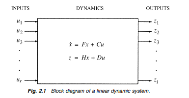
The block diagram in Figure $2.1$ represents a linear continuous system with three types of variables:

  • Inputs, which are under our control, and therefore known to us, or at least measurable by us. (In the next chapter, however, they will be assumed to be known only statistically. That is, individual samples of $u$ are random but with known statistical properties.)
  • State variables, which were described in the previous section. In most applications, these are “hidden variables,” in the sense that they cannot generally be measured directly but must be somehow inferred from what can be measured.
  • Outputs, which are those things that can be known through measurements.
    These concepts are discussed in greater detail in the following subsections.

数学代写|matlab代写|Dynamic Coefficient Matrices and Input Coupling Matrices

The dynamics of linear systems are represented by a set of $n$ first-order linear differential equations expressible in vector form as
$$
\begin{aligned}
\dot{x}(t) &=\frac{d}{d t} x(t) \
&=F(t) x(t)+C(t) u(t)
\end{aligned}
$$
where the elements and components of the matrices and vectors can be functions of time:
$$
\begin{aligned}
F(t)=& {\left[\begin{array}{ccccc}
f_{11}(t) & f_{12}(t) & f_{13}(t) & \cdots & f_{1 n}(t) \
f_{21}(t) & f_{22}(t) & f_{23}(t) & \cdots & f_{2 n}(t) \
f_{31}(t) & f_{32}(t) & f_{33}(t) & \cdots & f_{3 n}(t) \
\vdots & \vdots & \vdots & \ddots & \vdots \
f_{n 1}(t) & f_{n 2}(t) & f_{n 3}(t) & \cdots & f_{n n}(t)
\end{array}\right] } \
C(t)=& {\left[\begin{array}{ccccc}
c_{11}(t) & c_{12}(t) & c_{13}(t) & \cdots & c_{1 r}(t) \
c_{21}(t) & c_{22}(t) & c_{23}(t) & \cdots & c_{2 r}(t) \
c_{31}(t) & c_{32}(t) & c_{33}(t) & \cdots & c_{3 r}(t) \
\vdots & \vdots & \vdots & \ddots & \vdots \
c_{n 1}(t) & c_{n 2}(t) & c_{n 3}(t) & \cdots & c_{n r}(t)
\end{array}\right] } \
u(t)=& {\left[\begin{array}{lllll}
u_{1}(t) & u_{2}(t) & u_{3}(t) & \cdots & u_{r}(t)
\end{array}\right]^{\mathrm{T}} }
\end{aligned}
$$
The matrix $F(t)$ is called the dynamic coefficient matrix, or simply the dynamic matrix. Its elements are called the dynamic coefficients. The matrix $C(t)$ is called the input coupling matrix, and its elements are called input coupling coefficients. The $r$-vector $u$ is called the input vector.

数学代写|matlab代写|Difference Equations and State Transition Matrices

Difference equations are the discrete-time versions of differential equations. They are usually written in terms of forward differences $x\left(t_{k+1}\right)-x\left(t_{k}\right)$ of the state variable (the dependent variable), expressed as a function $\psi$ of all independent variables or of the forward value $x\left(t_{k+1}\right)$ as a function $\phi$ of all independent variables (including the previous value as an independent variable):
$$
x\left(t_{k+1}\right)-x\left(t_{k}\right)=\psi\left(t_{k}, x\left(t_{k}\right), u\left(t_{k}\right)\right)
$$
or
$$
\begin{gathered}
x\left(t_{k+1}\right)=\phi\left(t_{k}, x\left(t_{k}\right), u\left(t_{k}\right)\right), \
\phi\left(t_{k}, x\left(t_{k}\right), u\left(t_{k}\right)\right)=x\left(t_{k}\right)+\psi\left(t_{k}, x\left(t_{k}\right), u\left(t_{k}\right)\right) .
\end{gathered}
$$
The second of these (Equation 2.10) has the same general form of the recursive relation shown in Equation $2.4$, which is the one that is usually implemented for discrete-time systems.

For linear dynamic systems, the functional dependence of $x\left(t_{k+1}\right)$ on $x\left(t_{k}\right)$ and $u\left(t_{k}\right)$ can be represented by matrices:
$$
\begin{aligned}
x\left(t_{k+1}\right)-x\left(t_{k}\right) &=\Psi\left(t_{k}\right) x\left(t_{k}\right)+C\left(t_{k}\right) u\left(t_{k}\right), \
x_{k+1} &=\Phi_{k} x_{k}+C_{k} u_{k}, \
\Phi_{k} &=I+\Psi\left(t_{k}\right),
\end{aligned}
$$
where the matrices $\Psi$ and $\Phi$ replace the functions $\psi$ and $\phi$, respectively. The matrix $\Phi$ is called the state transition matrix $(S T M)$. The matrix $c$ is called the discrete-time input coupling matrix, or simply the input coupling matrix – if the discrete-time context is already established.

数学代写|matlab代写|CONTINUOUS LINEAR SYSTEMS AND THEIR SOLUTIONS

matlab代做

数学代写|matlab代写|Input-Output Models of Linear Dynamic Systems

框图如图2.1表示具有三种类型变量的线性连续系统:

  • 输入,在我们的控制之下,因此我们知道,或者至少我们可以测量。(然而,在下一章中,将假定它们仅在统计上已知。也就是说,在是随机的,但具有已知的统计特性。)
  • 状态变量,在上一节中进行了描述。在大多数应用程序中,这些是“隐藏变量”,因为它们通常不能直接测量,但必须以某种方式从可以测量的内容中推断出来。
  • 输出,即那些可以通过测量知道的东西。
    以下小节将更详细地讨论这些概念。

数学代写|matlab代写|Dynamic Coefficient Matrices and Input Coupling Matrices

线性系统的动力学由一组表示n一阶线性微分方程可表示为向量形式
X˙(吨)=dd吨X(吨) =F(吨)X(吨)+C(吨)在(吨)
其中矩阵和向量的元素和分量可以是时间的函数:
F(吨)=[F11(吨)F12(吨)F13(吨)⋯F1n(吨) F21(吨)F22(吨)F23(吨)⋯F2n(吨) F31(吨)F32(吨)F33(吨)⋯F3n(吨) ⋮⋮⋮⋱⋮ Fn1(吨)Fn2(吨)Fn3(吨)⋯Fnn(吨)] C(吨)=[C11(吨)C12(吨)C13(吨)⋯C1r(吨) C21(吨)C22(吨)C23(吨)⋯C2r(吨) C31(吨)C32(吨)C33(吨)⋯C3r(吨) ⋮⋮⋮⋱⋮ Cn1(吨)Cn2(吨)Cn3(吨)⋯Cnr(吨)] 在(吨)=[在1(吨)在2(吨)在3(吨)⋯在r(吨)]吨
矩阵F(吨)称为动态系数矩阵,或简称为动态矩阵。它的元素称为动态系数。矩阵C(吨)称为输入耦合矩阵,其元素称为输入耦合系数。这r-向量在称为输入向量。

数学代写|matlab代写|Difference Equations and State Transition Matrices

微分方程是微分方程的离散时间版本。它们通常用前向差异来写X(吨ķ+1)−X(吨ķ)状态变量(因变量),表示为函数ψ所有自变量或远期值X(吨ķ+1)作为一个函数φ所有自变量(包括以前的值作为自变量):
X(吨ķ+1)−X(吨ķ)=ψ(吨ķ,X(吨ķ),在(吨ķ))
或者
X(吨ķ+1)=φ(吨ķ,X(吨ķ),在(吨ķ)), φ(吨ķ,X(吨ķ),在(吨ķ))=X(吨ķ)+ψ(吨ķ,X(吨ķ),在(吨ķ)).
其中的第二个(等式 2.10)具有与等式所示的递归关系相同的一般形式2.4,这是通常为离散时间系统实现的一种。

对于线性动态系统,函数依赖性X(吨ķ+1)在X(吨ķ)和在(吨ķ)可以用矩阵表示:
X(吨ķ+1)−X(吨ķ)=Ψ(吨ķ)X(吨ķ)+C(吨ķ)在(吨ķ), Xķ+1=披ķXķ+Cķ在ķ, 披ķ=一世+Ψ(吨ķ),
矩阵在哪里Ψ和披替换函数ψ和φ, 分别。矩阵披称为状态转移矩阵(小号吨米). 矩阵C称为离散时间输入耦合矩阵,或简称为输入耦合矩阵——如果离散时间上下文已经建立。

数学代写|matlab代写 请认准statistics-lab™

统计代写请认准statistics-lab™. statistics-lab™为您的留学生涯保驾护航。

金融工程代写

金融工程是使用数学技术来解决金融问题。金融工程使用计算机科学、统计学、经济学和应用数学领域的工具和知识来解决当前的金融问题,以及设计新的和创新的金融产品。

非参数统计代写

非参数统计指的是一种统计方法,其中不假设数据来自于由少数参数决定的规定模型;这种模型的例子包括正态分布模型和线性回归模型。

广义线性模型代考

广义线性模型(GLM)归属统计学领域,是一种应用灵活的线性回归模型。该模型允许因变量的偏差分布有除了正态分布之外的其它分布。

术语 广义线性模型(GLM)通常是指给定连续和/或分类预测因素的连续响应变量的常规线性回归模型。它包括多元线性回归,以及方差分析和方差分析(仅含固定效应)。

有限元方法代写

有限元方法(FEM)是一种流行的方法,用于数值解决工程和数学建模中出现的微分方程。典型的问题领域包括结构分析、传热、流体流动、质量运输和电磁势等传统领域。

有限元是一种通用的数值方法,用于解决两个或三个空间变量的偏微分方程(即一些边界值问题)。为了解决一个问题,有限元将一个大系统细分为更小、更简单的部分,称为有限元。这是通过在空间维度上的特定空间离散化来实现的,它是通过构建对象的网格来实现的:用于求解的数值域,它有有限数量的点。边界值问题的有限元方法表述最终导致一个代数方程组。该方法在域上对未知函数进行逼近。[1] 然后将模拟这些有限元的简单方程组合成一个更大的方程系统,以模拟整个问题。然后,有限元通过变化微积分使相关的误差函数最小化来逼近一个解决方案。

tatistics-lab作为专业的留学生服务机构,多年来已为美国、英国、加拿大、澳洲等留学热门地的学生提供专业的学术服务,包括但不限于Essay代写,Assignment代写,Dissertation代写,Report代写,小组作业代写,Proposal代写,Paper代写,Presentation代写,计算机作业代写,论文修改和润色,网课代做,exam代考等等。写作范围涵盖高中,本科,研究生等海外留学全阶段,辐射金融,经济学,会计学,审计学,管理学等全球99%专业科目。写作团队既有专业英语母语作者,也有海外名校硕博留学生,每位写作老师都拥有过硬的语言能力,专业的学科背景和学术写作经验。我们承诺100%原创,100%专业,100%准时,100%满意。

随机分析代写


随机微积分是数学的一个分支,对随机过程进行操作。它允许为随机过程的积分定义一个关于随机过程的一致的积分理论。这个领域是由日本数学家伊藤清在第二次世界大战期间创建并开始的。

时间序列分析代写

随机过程,是依赖于参数的一组随机变量的全体,参数通常是时间。 随机变量是随机现象的数量表现,其时间序列是一组按照时间发生先后顺序进行排列的数据点序列。通常一组时间序列的时间间隔为一恒定值(如1秒,5分钟,12小时,7天,1年),因此时间序列可以作为离散时间数据进行分析处理。研究时间序列数据的意义在于现实中,往往需要研究某个事物其随时间发展变化的规律。这就需要通过研究该事物过去发展的历史记录,以得到其自身发展的规律。

回归分析代写

多元回归分析渐进(Multiple Regression Analysis Asymptotics)属于计量经济学领域,主要是一种数学上的统计分析方法,可以分析复杂情况下各影响因素的数学关系,在自然科学、社会和经济学等多个领域内应用广泛。

MATLAB代写

MATLAB 是一种用于技术计算的高性能语言。它将计算、可视化和编程集成在一个易于使用的环境中,其中问题和解决方案以熟悉的数学符号表示。典型用途包括:数学和计算算法开发建模、仿真和原型制作数据分析、探索和可视化科学和工程图形应用程序开发,包括图形用户界面构建MATLAB 是一个交互式系统,其基本数据元素是一个不需要维度的数组。这使您可以解决许多技术计算问题,尤其是那些具有矩阵和向量公式的问题,而只需用 C 或 Fortran 等标量非交互式语言编写程序所需的时间的一小部分。MATLAB 名称代表矩阵实验室。MATLAB 最初的编写目的是提供对由 LINPACK 和 EISPACK 项目开发的矩阵软件的轻松访问,这两个项目共同代表了矩阵计算软件的最新技术。MATLAB 经过多年的发展,得到了许多用户的投入。在大学环境中,它是数学、工程和科学入门和高级课程的标准教学工具。在工业领域,MATLAB 是高效研究、开发和分析的首选工具。MATLAB 具有一系列称为工具箱的特定于应用程序的解决方案。对于大多数 MATLAB 用户来说非常重要,工具箱允许您学习应用专业技术。工具箱是 MATLAB 函数(M 文件)的综合集合,可扩展 MATLAB 环境以解决特定类别的问题。可用工具箱的领域包括信号处理、控制系统、神经网络、模糊逻辑、小波、仿真等。

R语言代写问卷设计与分析代写
PYTHON代写回归分析与线性模型代写
MATLAB代写方差分析与试验设计代写
STATA代写机器学习/统计学习代写
SPSS代写计量经济学代写
EVIEWS代写时间序列分析代写
EXCEL代写深度学习代写
SQL代写各种数据建模与可视化代写

数学代写|matlab代写|Linear Dynamic Systems

如果你也在 怎样代写matlab这个学科遇到相关的难题,请随时右上角联系我们的24/7代写客服。

matlab是一个编程和数值计算平台,被数百万工程师和科学家用来分析数据、开发算法和创建模型。

statistics-lab™ 为您的留学生涯保驾护航 在代写matlab方面已经树立了自己的口碑, 保证靠谱, 高质且原创的统计Statistics代写服务。我们的专家在代写matlab代写方面经验极为丰富,各种代写matlab相关的作业也就用不着说。

我们提供的matlab及其相关学科的代写,服务范围广, 其中包括但不限于:

  • Statistical Inference 统计推断
  • Statistical Computing 统计计算
  • Advanced Probability Theory 高等楖率论
  • Advanced Mathematical Statistics 高等数理统计学
  • (Generalized) Linear Models 广义线性模型
  • Statistical Machine Learning 统计机器学习
  • Longitudinal Data Analysis 纵向数据分析
  • Foundations of Data Science 数据科学基础
Error Detection & Correction
数学代写|matlab代写|Linear Dynamic Systems

数学代写|matlab代写|Dynamic Systems Represented by Differential Equations

A system is an assemblage of interrelated entities that can be considered as a whole. If the attributes of interest of a system are changing with time, then it is called a dynamic system. A process is the evolution over time of a dynamic system.

Our solar system, consisting of the sun and its planets, is a physical example of a dynamic system. The motions of these bodies are governed by laws of motion that depend only upon their current relative positions and velocities. Sir Isaac Newton (1642-1727) discovered these laws and expressed them as a system of differential equations-another of his discoveries. From the time of Newton, engineers and scientists have learned to define dynamic systems in terms of the differential equations that govern their behavior. They have also learned how to solve many of these differential equations to obtain formulas for predicting the future behavior of dynamic systems.

EXAMPLE $2.1$ (below, left): Newton’s Model for a Dynamic System of $\boldsymbol{n}$ Massive Bodies For a planetary system with $n$ bodies (idealized as point masses), the acceleration of the $i$ th body in any inertial (i.e., non-rotating and non-accelerating) Cartesian coordinate system is given by Newton’s third law as the second-order differential equation
$$
\frac{d^{2} r_{i}}{d t^{2}}=C_{g} \sum_{\substack{j=1 \ j / i}}^{n} \frac{m_{j}\left[r_{j}-r_{i}\right]}{\left|r_{j}-r_{i}\right|^{3}}, 1 \leq i \leq n
$$
where $r_{j}$ is the position coordinate vector of the $j$ th body, $m_{j}$ is the mass of the $j$ th body, and $C_{g}$ is the gravitational constant. This set of $n$ differential equations, plus the associated initial conditions of the bodies (i.e., their initial positions and velocities) theoretically determines the future history of the planetary system.

数学代写|matlab代写|State Variables and State Equations

The second-order differential equation of the previous example can be transformed to a system of two first-order differential equations in the two dependent variables $x_{1}=\delta$ and $x_{2}=d \delta / d t$. In this way, one can reduce the form of any system of higher order differential equations to an equivalent system of first-order differential equations. These systems are generally classified into the types shown in Table 2.1, with the most general type being a time-varying differential equation for representing a dynamic system with time-varying dynamic characteristics. This is represented in vector form as
$$
\dot{x}(t)=f(t, x(t), u(t)),
$$
where Newton’s “dot” notation is used as a shorthand for the derivative with respect to time, and a vector-valued function $f$ to represent a system of $n$ equations
$$
\begin{aligned}
\dot{x}{1} &=f{1}\left(t, x_{1}, x_{2}, x_{3}, \ldots, x_{n}, u_{1}, u_{2}, u_{3}, \ldots, u_{r}, t\right), \
\dot{x}{2} &=f{2}\left(t, x_{1}, x_{2}, x_{3}, \ldots, x_{n}, u_{1}, u_{2}, u_{3}, \ldots, u_{r}, t\right), \
\dot{x}{3} &=f{3}\left(t, x_{1}, x_{2}, x_{3}, \ldots, x_{n}, u_{1}, u_{2}, u_{3}, \ldots, u_{r}, t\right), \
& \vdots \
\dot{x}{n} &=f{n}\left(t, x_{1}, x_{2}, x_{3}, \ldots, x_{n}, u_{1}, u_{2}, u_{3}, \ldots, u_{r}, t\right)
\end{aligned}
$$
in the independent variable $t$ (time), $n$ dependent variables $\left{x_{i} \mid 1 \leq i \leq n\right}$, and $r$ known inputs $\left{u_{i} \mid 1 \leq i \leq r\right}$. These are called the state equations of the dynamic system.

数学代写|matlab代写|Continuous Time and Discrete Time

The dynamic system defined by Equation $2.2$ is an example of a continuous system, so called because it is defined with respect to an independent variable $t$ that varies continuously over some real interval $t \in\left[t_{0}, t_{f}\right]$. For many practical problems, however, one is only interested in knowing the state of a system at a discrete set of times $t \in\left{t_{1}, t_{2}, t_{3}, \ldots\right}$. These discrete times may, for example, correspond to the times at which the outputs of a system are sampled (such as the times at which Piazzi recorded the direction to Ceres). For problems of this type, it is convenient to order the times $t_{k}$ according to their integer subscripts:
$$
t_{0}<t_{1}<t_{2}<\cdots t_{k-1}<t_{k}<t_{k+1}<\cdots .
$$

That is, the time sequence is ordered according to the subscripts, and the subscripts take on all successive values in some range of integers. For problems of this type, it suffices to define the state of the dynamic system as a recursive relation,
$$
x\left(t_{k+1}\right)=f\left(x\left(t_{k}\right), t_{k}, t_{k+1}\right),
$$
by means of which the state is represented as a function of its previous state. This is a definition of a discrete dynamic system. For systems with uniform time intervals $\Delta t$
$$
t_{k}=k \Delta t .
$$

数学代写|matlab代写|Linear Dynamic Systems

matlab代做

数学代写|matlab代写|Dynamic Systems Represented by Differential Equations

系统是可以被视为一个整体的相互关联的实体的集合。如果一个系统感兴趣的属性随时间变化,则称为动态系统。过程是动态系统随时间的演变。

我们的太阳系由太阳及其行星组成,是动态系统的物理示例。这些物体的运动受运动定律支配,这些定律仅取决于它们当前的相对位置和速度。艾萨克·牛顿爵士 (1642-1727) 发现了这些定律并将它们表达为微分方程系统——他的另一个发现。从牛顿时代开始,工程师和科学家就已经学会根据控制其行为的微分方程来定义动态系统。他们还学会了如何求解这些微分方程,以获得预测动态系统未来行为的公式。

例子2.1(下,左):牛顿的动态系统模型n大质量行星系统n物体(理想化为点质量),加速度一世任何惯性(即非旋转和非加速)笛卡尔坐标系中的物体由牛顿第三定律作为二阶微分方程给出
d2r一世d吨2=CG∑j=1 j/一世n米j[rj−r一世]|rj−r一世|3,1≤一世≤n
在哪里rj是位置坐标向量j身体,米j是质量j身体,和CG是引力常数。这一套n微分方程,加上相关的天体初始条件(即,它们的初始位置和速度)在理论上决定了行星系统的未来历史。

数学代写|matlab代写|State Variables and State Equations

上例的二阶微分方程可以转化为两个因变量中的两个一阶微分方程组X1=d和X2=dd/d吨. 通过这种方式,可以将任何高阶微分方程组的形式简化为等价的一阶微分方程组。这些系统一般分为表 2.1 所示的类型,最通用的类​​型是用于表示具有时变动态特性的动态系统的时变微分方程。这以向量形式表示为
X˙(吨)=F(吨,X(吨),在(吨)),
其中牛顿的“点”符号用作关于时间的导数的简写,以及向量值函数F表示一个系统n方程
X˙1=F1(吨,X1,X2,X3,…,Xn,在1,在2,在3,…,在r,吨), X˙2=F2(吨,X1,X2,X3,…,Xn,在1,在2,在3,…,在r,吨), X˙3=F3(吨,X1,X2,X3,…,Xn,在1,在2,在3,…,在r,吨), ⋮ X˙n=Fn(吨,X1,X2,X3,…,Xn,在1,在2,在3,…,在r,吨)
在自变量中吨(时间),n因变量\left{x_{i} \mid 1 \leq i \leq n\right}\left{x_{i} \mid 1 \leq i \leq n\right}, 和r已知输入\left{u_{i} \mid 1 \leq i \leq r\right}\left{u_{i} \mid 1 \leq i \leq r\right}. 这些被称为动态系统的状态方程。

数学代写|matlab代写|Continuous Time and Discrete Time

方程定义的动态系统2.2是一个连续系统的例子,之所以这么称呼它是因为它是关于一个自变量定义的吨在某个实际间隔内连续变化吨∈[吨0,吨F]. 然而,对于许多实际问题,人们只对了解系统在一组离散时间的状态感兴趣t \in\left{t_{1}, t_{2}, t_{3}, \ldots\right}t \in\left{t_{1}, t_{2}, t_{3}, \ldots\right}. 例如,这些离散时间可能对应于对系统输出进行采样的时间(例如 Piazzi 记录到 Ceres 的方向的时间)。此类问题,方便下单时间吨ķ根据它们的整数下标:
吨0<吨1<吨2<⋯吨ķ−1<吨ķ<吨ķ+1<⋯.

即时间序列按照下标排序,下标取某个整数范围内的所有连续值。对于这种类型的问题,将动态系统的状态定义为递归关系就足够了,
X(吨ķ+1)=F(X(吨ķ),吨ķ,吨ķ+1),
通过它,状态被表示为其先前状态的函数。这是离散动态系统的定义。对于具有统一时间间隔的系统Δ吨
吨ķ=ķΔ吨.

数学代写|matlab代写 请认准statistics-lab™

统计代写请认准statistics-lab™. statistics-lab™为您的留学生涯保驾护航。

金融工程代写

金融工程是使用数学技术来解决金融问题。金融工程使用计算机科学、统计学、经济学和应用数学领域的工具和知识来解决当前的金融问题,以及设计新的和创新的金融产品。

非参数统计代写

非参数统计指的是一种统计方法,其中不假设数据来自于由少数参数决定的规定模型;这种模型的例子包括正态分布模型和线性回归模型。

广义线性模型代考

广义线性模型(GLM)归属统计学领域,是一种应用灵活的线性回归模型。该模型允许因变量的偏差分布有除了正态分布之外的其它分布。

术语 广义线性模型(GLM)通常是指给定连续和/或分类预测因素的连续响应变量的常规线性回归模型。它包括多元线性回归,以及方差分析和方差分析(仅含固定效应)。

有限元方法代写

有限元方法(FEM)是一种流行的方法,用于数值解决工程和数学建模中出现的微分方程。典型的问题领域包括结构分析、传热、流体流动、质量运输和电磁势等传统领域。

有限元是一种通用的数值方法,用于解决两个或三个空间变量的偏微分方程(即一些边界值问题)。为了解决一个问题,有限元将一个大系统细分为更小、更简单的部分,称为有限元。这是通过在空间维度上的特定空间离散化来实现的,它是通过构建对象的网格来实现的:用于求解的数值域,它有有限数量的点。边界值问题的有限元方法表述最终导致一个代数方程组。该方法在域上对未知函数进行逼近。[1] 然后将模拟这些有限元的简单方程组合成一个更大的方程系统,以模拟整个问题。然后,有限元通过变化微积分使相关的误差函数最小化来逼近一个解决方案。

tatistics-lab作为专业的留学生服务机构,多年来已为美国、英国、加拿大、澳洲等留学热门地的学生提供专业的学术服务,包括但不限于Essay代写,Assignment代写,Dissertation代写,Report代写,小组作业代写,Proposal代写,Paper代写,Presentation代写,计算机作业代写,论文修改和润色,网课代做,exam代考等等。写作范围涵盖高中,本科,研究生等海外留学全阶段,辐射金融,经济学,会计学,审计学,管理学等全球99%专业科目。写作团队既有专业英语母语作者,也有海外名校硕博留学生,每位写作老师都拥有过硬的语言能力,专业的学科背景和学术写作经验。我们承诺100%原创,100%专业,100%准时,100%满意。

随机分析代写


随机微积分是数学的一个分支,对随机过程进行操作。它允许为随机过程的积分定义一个关于随机过程的一致的积分理论。这个领域是由日本数学家伊藤清在第二次世界大战期间创建并开始的。

时间序列分析代写

随机过程,是依赖于参数的一组随机变量的全体,参数通常是时间。 随机变量是随机现象的数量表现,其时间序列是一组按照时间发生先后顺序进行排列的数据点序列。通常一组时间序列的时间间隔为一恒定值(如1秒,5分钟,12小时,7天,1年),因此时间序列可以作为离散时间数据进行分析处理。研究时间序列数据的意义在于现实中,往往需要研究某个事物其随时间发展变化的规律。这就需要通过研究该事物过去发展的历史记录,以得到其自身发展的规律。

回归分析代写

多元回归分析渐进(Multiple Regression Analysis Asymptotics)属于计量经济学领域,主要是一种数学上的统计分析方法,可以分析复杂情况下各影响因素的数学关系,在自然科学、社会和经济学等多个领域内应用广泛。

MATLAB代写

MATLAB 是一种用于技术计算的高性能语言。它将计算、可视化和编程集成在一个易于使用的环境中,其中问题和解决方案以熟悉的数学符号表示。典型用途包括:数学和计算算法开发建模、仿真和原型制作数据分析、探索和可视化科学和工程图形应用程序开发,包括图形用户界面构建MATLAB 是一个交互式系统,其基本数据元素是一个不需要维度的数组。这使您可以解决许多技术计算问题,尤其是那些具有矩阵和向量公式的问题,而只需用 C 或 Fortran 等标量非交互式语言编写程序所需的时间的一小部分。MATLAB 名称代表矩阵实验室。MATLAB 最初的编写目的是提供对由 LINPACK 和 EISPACK 项目开发的矩阵软件的轻松访问,这两个项目共同代表了矩阵计算软件的最新技术。MATLAB 经过多年的发展,得到了许多用户的投入。在大学环境中,它是数学、工程和科学入门和高级课程的标准教学工具。在工业领域,MATLAB 是高效研究、开发和分析的首选工具。MATLAB 具有一系列称为工具箱的特定于应用程序的解决方案。对于大多数 MATLAB 用户来说非常重要,工具箱允许您学习应用专业技术。工具箱是 MATLAB 函数(M 文件)的综合集合,可扩展 MATLAB 环境以解决特定类别的问题。可用工具箱的领域包括信号处理、控制系统、神经网络、模糊逻辑、小波、仿真等。

R语言代写问卷设计与分析代写
PYTHON代写回归分析与线性模型代写
MATLAB代写方差分析与试验设计代写
STATA代写机器学习/统计学习代写
SPSS代写计量经济学代写
EVIEWS代写时间序列分析代写
EXCEL代写深度学习代写
SQL代写各种数据建模与可视化代写

数学代写|matlab代写|ON THE NOTATION USED IN THIS BOOK

如果你也在 怎样代写matlab这个学科遇到相关的难题,请随时右上角联系我们的24/7代写客服。

matlab是一个编程和数值计算平台,被数百万工程师和科学家用来分析数据、开发算法和创建模型。

statistics-lab™ 为您的留学生涯保驾护航 在代写matlab方面已经树立了自己的口碑, 保证靠谱, 高质且原创的统计Statistics代写服务。我们的专家在代写matlab代写方面经验极为丰富,各种代写matlab相关的作业也就用不着说。

我们提供的matlab及其相关学科的代写,服务范围广, 其中包括但不限于:

  • Statistical Inference 统计推断
  • Statistical Computing 统计计算
  • Advanced Probability Theory 高等楖率论
  • Advanced Mathematical Statistics 高等数理统计学
  • (Generalized) Linear Models 广义线性模型
  • Statistical Machine Learning 统计机器学习
  • Longitudinal Data Analysis 纵向数据分析
  • Foundations of Data Science 数据科学基础
数学代写|matlab代写|ON THE NOTATION USED IN THIS BOOK

数学代写|matlab代写|Symbolic Notation

The fundamental problem of symbolic notation, in almost any context, is that there are never enough symbols to go around. There are not enough letters in the Roman alphabet to represent the sounds of standard English, let alone all the variables in Kalman filtering and its applications. As a result, some symbols must play multiple roles. In such cases, their roles will be defined as they are introduced. It is sometimes confusing, but unavoidable.

“Dot”‘ Notation for Derivatives. Newton’s notation using $\vec{f}(t), \vec{f}(t)$ for the first two derivatives of $f$ with respect to $t$ is used where convenient to save ink.

Standard Symbols for Kalman Filter Variables. There appear to be two “standard” conventions in technical publications for the symbols used in Kalman filtering. The one used in this book is similar to the original notation of Kalman [179]. The other standard notation is sometimes associated with applications of Kalman filtering in control theory. It uses the first few letters of the alphabet in place of the Kalman notation. Both sets of symbol usages are presented in Table 1.2, along with the original (Kalman) notation.

State Vector Notation for Kalman Filtering. The state vector $x$ has been adorned with all sorts of other appendages in the usage of Kalman filtering. Table $1.3$ lists the notation used in this book (left column) along with notations found in some other sources (second column). The state vector wears a “hat” as the estimated value, $\hat{x}$, and subscripting to denote the sequence of values that the estimate assumes over time. The problem is that it has two values at the same time: the a priori ${ }^{17}$ value (before the measurement at the current time has been used in refining the estimate) and the a posteriori value (after the current measurement has been used in refining the estimate). These distinctions are indicated by the signum. The negative sign $(-)$ indicates the a priori value, and the positive sign $(+)$ indicates the a posteriori value.

数学代写|matlab代写|SUMMARY

The Kalman filter is an estimator used to estimate the state of a linear dynamic system perturbed by Gaussian white noise using measurements that are linear functions of the system state but corrupted by additive Gaussian white noise. The mathematical model used in the derivation of the Kalman filter is a reasonable representation for many problems of practical interest, including control problems as

well as estimation problems. The Kalman filter model is also used for the analysis of measurement and estimation problems.

The method of least squares was the first “optimal” estimation method. It was discovered by Gauss (and others) around the end of the eighteenth century, and it is still much in use today. If the associated Gramian matrix is nonsingular, the method of least squares determines the unique values of a set of unknown variables such that the squared deviation from a set of constraining equations is minimized.

Observability of a set of unknown variables is the issue of whether or not they are uniquely determinable from a given set of constraining equations. If the constraints are linear functions of the unknown variables, then those variables are observable if and only if the associated Gramian matrix is nonsingular. If the Gramian matrix is singular, then the unknown variables are unobservable.

The Wiener-Kolmogorov filter was derived in the $1940 \mathrm{~s}$ by Norbert Wiener (using a model in continuous time) and Andrei Kolmogorov (using a model in discrete time) working independently. It is a statistical estimation method. It estimates the state of a dynamic process so as to minimize the mean-squared estimation error. It can take advantage of statistical knowledge about random processes in terms of their power spectral densities in the frequency domain.

The “state-space” model of a dynamic process uses differential equations (or difference equations) to represent both deterministic and random phenomena. The state variables of this model are the variables of interest and their derivatives of interest. Random processes are characterized in terms of their statistical properties in the time domain, rather than the frequency domain. The Kalman filter was derived as the solution to the Wiener filtering problem using the state-space model for dynamic and random processes. The result is easier to derive (and to use) than the WienerKolmogorov filter.

Square-root filtering is a reformulation of the Kalman filter for better numerical stability in finite-precision arithmetic. It is based on the same mathematical model, but it uses an equivalent statistical parameter that is less sensitive to roundoff errors in the computation of optimal filter gains. It incorporates many of the more numerically stable computation methods that were originally derived for solving the least-squares problem.

数学代写|matlab代写|CHAPTER FOCUS

Models for Dynamic Systems. Since their introduction by Isaac Newton in the seventeenth century, differential equations have provided concise mathematical models for many dynamic systems of importance to humans. By this device, Newton was able to model the motions of the planets in our solar system with a small number of variables and parameters. Given a finite number of initial conditions (the initial positions and velocities of the sun and planets will do) and these equations, one can uniquely determine the positions and velocities of the planets for all time. The finite-dimensional representation of a problem (in this example, the problem of predicting the future course of the planets) is the basis for the so-called state-space approach to the representation of differential equations and their solutions, which is the focus of this chapter. The dependent variables of the differential equations become state variables of the dynamic system. They explicitly represent all the important characteristics of the dynamic system at any time.

The whole of dynamic system theory is a subject of considerably more scope than one needs for the present undertaking (Kalman filtering). This chapter will stick to just those concepts that are essential for that purpose, which is the development of the statespace representation for dynamic systems described by systems of linear differential equations. These are given a somewhat heuristic treatment, without the mathematical rigor often accorded the subject, omitting the development and use of the transform methods of functional analysis for solving differential equations when they serve no purpose in the derivation of the Kalman filter. The interested reader will find a more formal and thorough presentation in most upper-level and graduate-level textbooks on ordinary differential equations. The objective of the more engineering-oriented treatments of dynamic systems is usually to solve the controls problem, which is the problem of defining the inputs (i.e., control settings) that will bring the state of the dynamic system to a desirable condition. That is not the objective here, however.

The initial problem geometry for scale detection implemented in MCNP5.... |  Download Scientific Diagram
数学代写|matlab代写|ON THE NOTATION USED IN THIS BOOK

matlab代做

数学代写|matlab代写|Symbolic Notation

几乎在任何情况下,符号表示法的基本问题是永远没有足够的符号可以传播。罗马字母表中没有足够的字母来表示标准英语的发音,更不用说卡尔曼滤波及其应用中的所有变量了。因此,一些符号必须扮演多重角色。在这种情况下,他们的角色将在介绍时定义。这有时令人困惑,但不可避免。

导数的“点”符号。牛顿符号使用F→(吨),F→(吨)对于前两个导数F关于吨用于方便节省墨水的地方。

卡尔曼滤波器变量的标准符号。对于卡尔曼滤波中使用的符号,技术出版物中似乎有两个“标准”约定。本书中使用的符号类似于 Kalman [179] 的原始符号。另一种标准符号有时与卡尔曼滤波在控制理论中的应用有关。它使用字母表的前几个字母代替卡尔曼符号。表 1.2 中列出了两组符号的用法,以及原始 (Kalman) 符号。

卡尔曼滤波的状态向量表示法。状态向量X在卡尔曼滤波的使用中,已经装饰了各种其他附件。桌子1.3列出了本书中使用的符号(左栏)以及在其他一些来源中找到的符号(第二栏)。状态向量戴上“帽子”作为估计值,X^, 和下标表示估计随时间假设的值序列。问题是它同时有两个值:先验17值(在当前时间的测量被用于细化估计之前)和后验值(在当前测量被用于细化估计之后)。这些区别由符号表示。负号(−)表示先验值,正号(+)表示后验值。

数学代写|matlab代写|SUMMARY

卡尔曼滤波器是一种估计器,用于估计受高斯白噪声干扰的线性动态系统的状态,使用的测量值是系统状态的线性函数,但被加性高斯白噪声破坏。用于推导卡尔曼滤波器的数学模型是许多实际问题的合理表示,包括控制问题

以及估计问题。卡尔曼滤波器模型也用于分析测量和估计问题。

最小二乘法是第一个“最优”估计方法。它是在 18 世纪末由 Gauss(和其他人)发现的,至今仍在大量使用。如果相关的 Gramian 矩阵是非奇异的,则最小二乘法确定一组未知变量的唯一值,以使与一组约束方程的平方偏差最小化。

一组未知变量的可观测性是它们是否可以从给定的一组约束方程中唯一确定的问题。如果约束是未知变量的线性函数,那么当且仅当相关的 Gramian 矩阵是非奇异的时,这些变量是可观察的。如果 Gramian 矩阵是奇异的,则未知变量是不可观测的。

Wiener-Kolmogorov 滤波器由1940 s由 Norbert Wiener(使用连续时间的模型)和 Andrei Kolmogorov(使用离散时间的模型)独立工作。它是一种统计估计方法。它估计动态过程的状态,以最小化均方估计误差。它可以利用随机过程在频域中的功率谱密度方面的统计知识。

动态过程的“状态空间”模型使用微分方程(或差分方程)来表示确定性和随机现象。该模型的状态变量是感兴趣的变量及其感兴趣的导数。随机过程的特征在于它们在时域而不是频域中的统计特性。卡尔曼滤波器是使用动态和随机过程的状态空间模型来解决维纳滤波问题的。结果比 WienerKolmogorov 滤波器更容易推导(和使用)。

平方根滤波是卡尔曼滤波器的重新表述,用于在有限精度算术中获得更好的数值稳定性。它基于相同的数学模型,但在计算最佳滤波器增益时使用了对舍入误差不太敏感的等效统计参数。它结合了许多最初为解决最小二乘问题而导出的数值更稳定的计算方法。

数学代写|matlab代写|CHAPTER FOCUS

动态系统模型。自从 17 世纪艾萨克·牛顿引入微分方程以来,微分方程已经为许多对人类重要的动态系统提供了简明的数学模型。通过这个设备,牛顿能够用少量变量和参数模拟太阳系中行星的运动。给定有限数量的初始条件(太阳和行星的初始位置和速度可以)和这些方程,人们可以始终唯一地确定行星的位置和速度。问题的有限维表示(在这个例子中,是预测行星未来轨迹的问题)是表示微分方程及其解的所谓状态空间方法的基础,这是重点本章的。微分方程的因变量成为动态系统的状态变量。它们在任何时候都明确地代表了动态系统的所有重要特征。

整个动态系统理论是一门比当前工作(卡尔曼滤波)需要的范围大得多的主题。本章将只关注那些为此目的必不可少的概念,即发展由线性微分方程系统描述的动态系统的状态空间表示。这些被给予了某种启发式的处理,没有通常给予该主题的数学严谨性,省略了用于求解微分方程的泛函分析变换方法的开发和使用,当它们在卡尔曼滤波器的推导中无用时。感兴趣的读者会在大多数关于常微分方程的高级和研究生教科书中找到更正式和更全面的介绍。更面向工程的动态系统处理的目标通常是解决控制问题,即定义将动态系统的状态带到理想状态的输入(即控制设置)的问题。然而,这不是这里的目标。

数学代写|matlab代写 请认准statistics-lab™

统计代写请认准statistics-lab™. statistics-lab™为您的留学生涯保驾护航。

金融工程代写

金融工程是使用数学技术来解决金融问题。金融工程使用计算机科学、统计学、经济学和应用数学领域的工具和知识来解决当前的金融问题,以及设计新的和创新的金融产品。

非参数统计代写

非参数统计指的是一种统计方法,其中不假设数据来自于由少数参数决定的规定模型;这种模型的例子包括正态分布模型和线性回归模型。

广义线性模型代考

广义线性模型(GLM)归属统计学领域,是一种应用灵活的线性回归模型。该模型允许因变量的偏差分布有除了正态分布之外的其它分布。

术语 广义线性模型(GLM)通常是指给定连续和/或分类预测因素的连续响应变量的常规线性回归模型。它包括多元线性回归,以及方差分析和方差分析(仅含固定效应)。

有限元方法代写

有限元方法(FEM)是一种流行的方法,用于数值解决工程和数学建模中出现的微分方程。典型的问题领域包括结构分析、传热、流体流动、质量运输和电磁势等传统领域。

有限元是一种通用的数值方法,用于解决两个或三个空间变量的偏微分方程(即一些边界值问题)。为了解决一个问题,有限元将一个大系统细分为更小、更简单的部分,称为有限元。这是通过在空间维度上的特定空间离散化来实现的,它是通过构建对象的网格来实现的:用于求解的数值域,它有有限数量的点。边界值问题的有限元方法表述最终导致一个代数方程组。该方法在域上对未知函数进行逼近。[1] 然后将模拟这些有限元的简单方程组合成一个更大的方程系统,以模拟整个问题。然后,有限元通过变化微积分使相关的误差函数最小化来逼近一个解决方案。

tatistics-lab作为专业的留学生服务机构,多年来已为美国、英国、加拿大、澳洲等留学热门地的学生提供专业的学术服务,包括但不限于Essay代写,Assignment代写,Dissertation代写,Report代写,小组作业代写,Proposal代写,Paper代写,Presentation代写,计算机作业代写,论文修改和润色,网课代做,exam代考等等。写作范围涵盖高中,本科,研究生等海外留学全阶段,辐射金融,经济学,会计学,审计学,管理学等全球99%专业科目。写作团队既有专业英语母语作者,也有海外名校硕博留学生,每位写作老师都拥有过硬的语言能力,专业的学科背景和学术写作经验。我们承诺100%原创,100%专业,100%准时,100%满意。

随机分析代写


随机微积分是数学的一个分支,对随机过程进行操作。它允许为随机过程的积分定义一个关于随机过程的一致的积分理论。这个领域是由日本数学家伊藤清在第二次世界大战期间创建并开始的。

时间序列分析代写

随机过程,是依赖于参数的一组随机变量的全体,参数通常是时间。 随机变量是随机现象的数量表现,其时间序列是一组按照时间发生先后顺序进行排列的数据点序列。通常一组时间序列的时间间隔为一恒定值(如1秒,5分钟,12小时,7天,1年),因此时间序列可以作为离散时间数据进行分析处理。研究时间序列数据的意义在于现实中,往往需要研究某个事物其随时间发展变化的规律。这就需要通过研究该事物过去发展的历史记录,以得到其自身发展的规律。

回归分析代写

多元回归分析渐进(Multiple Regression Analysis Asymptotics)属于计量经济学领域,主要是一种数学上的统计分析方法,可以分析复杂情况下各影响因素的数学关系,在自然科学、社会和经济学等多个领域内应用广泛。

MATLAB代写

MATLAB 是一种用于技术计算的高性能语言。它将计算、可视化和编程集成在一个易于使用的环境中,其中问题和解决方案以熟悉的数学符号表示。典型用途包括:数学和计算算法开发建模、仿真和原型制作数据分析、探索和可视化科学和工程图形应用程序开发,包括图形用户界面构建MATLAB 是一个交互式系统,其基本数据元素是一个不需要维度的数组。这使您可以解决许多技术计算问题,尤其是那些具有矩阵和向量公式的问题,而只需用 C 或 Fortran 等标量非交互式语言编写程序所需的时间的一小部分。MATLAB 名称代表矩阵实验室。MATLAB 最初的编写目的是提供对由 LINPACK 和 EISPACK 项目开发的矩阵软件的轻松访问,这两个项目共同代表了矩阵计算软件的最新技术。MATLAB 经过多年的发展,得到了许多用户的投入。在大学环境中,它是数学、工程和科学入门和高级课程的标准教学工具。在工业领域,MATLAB 是高效研究、开发和分析的首选工具。MATLAB 具有一系列称为工具箱的特定于应用程序的解决方案。对于大多数 MATLAB 用户来说非常重要,工具箱允许您学习应用专业技术。工具箱是 MATLAB 函数(M 文件)的综合集合,可扩展 MATLAB 环境以解决特定类别的问题。可用工具箱的领域包括信号处理、控制系统、神经网络、模糊逻辑、小波、仿真等。

R语言代写问卷设计与分析代写
PYTHON代写回归分析与线性模型代写
MATLAB代写方差分析与试验设计代写
STATA代写机器学习/统计学习代写
SPSS代写计量经济学代写
EVIEWS代写时间序列分析代写
EXCEL代写深度学习代写
SQL代写各种数据建模与可视化代写

数学代写|matlab代写|Square-Root Methods and All That

如果你也在 怎样代写matlab这个学科遇到相关的难题,请随时右上角联系我们的24/7代写客服。

matlab是一个编程和数值计算平台,被数百万工程师和科学家用来分析数据、开发算法和创建模型。

statistics-lab™ 为您的留学生涯保驾护航 在代写matlab方面已经树立了自己的口碑, 保证靠谱, 高质且原创的统计Statistics代写服务。我们的专家在代写matlab代写方面经验极为丰富,各种代写matlab相关的作业也就用不着说。

我们提供的matlab及其相关学科的代写,服务范围广, 其中包括但不限于:

  • Statistical Inference 统计推断
  • Statistical Computing 统计计算
  • Advanced Probability Theory 高等楖率论
  • Advanced Mathematical Statistics 高等数理统计学
  • (Generalized) Linear Models 广义线性模型
  • Statistical Machine Learning 统计机器学习
  • Longitudinal Data Analysis 纵向数据分析
  • Foundations of Data Science 数据科学基础
数学代写|matlab代写|Square-Root Methods and All That

数学代写|matlab代写|Numerical Stability Problems

Numerical Stability Problems. The great success of Kalman filtering was not without its problems, not the least of which was marginal stability of the numerical solution of the associated Riccati equation. In some applications, small roundoff errors tended to accumulate and eventually degrade the performance of the filter. In the decades immediately following the introduction of the Kalman filter, there appeared several better numerical implementations of the original formulas. Many of these were adaptations of methods previously derived for the least squares problem.
Early ad hoc Fixes. It was discovered early on ${ }^{13}$ that forcing symmetry on the solution of the matrix Riccati equation improved its apparent numerical stability-a phenomenon that was later given a more theoretical basis by Verhaegen and Van Dooren [232]. It was also found that the influence of roundoff errors could be ameliorated by artificially increasing the covariance of process noise in the Riccati equation. A symmetrized form of the discrete-time Riccati equation was developed by Joseph [15] and used by R. C. K. Lee at Honeywell in 1964. This “structural” reformulation of the Kalman filter equations improved robustness against roundoff errors in some applications, although later methods have performed better on some problems [125].

Square-Root Filtering. These methods can also be considered as “structural” reformulations of the Riccati equation, and they predate the Bucy-Joseph form. The first of these was the “square-root” implementation by Potter and Stern [208], first published in 1963 and successfully implemented for space navigation on the Apollo manned lunar exploration program. Potter and Stern introduced the idea of factoring the covariance matrix into Cholesky factors, ${ }^{14}$ in the format
$$
P=C C^{\mathrm{T}}
$$
and expressing the observational update equations in terms of the Cholesky factor $C$, rather than $P$. The result was better numerical stability of the filter implementation at the expense of added computational complexity. A generalization of the Potter and Stern method to handle vector-valued measurements was published by one of the authors [130] in 1968 , but a more efficient implementation-in terms of triangular Cholesky factors – was published by Bennet in 1967 [138].

数学代写|matlab代写|Beyond Kalman Filtering

Extended Kalman Filtering and the Kalman-Schmidt Filter. Although it was originally derived for a linear problem, the Kalman filter is habitually applied with impunity-and considerable success – to many nonlinear problems. These extensions generally use partial derivatives as linear approximations of nonlinear relations. Schmidt [118] introduced the idea of evaluating these partial derivatives at the estimated value of the state variables. This approach is generally called the extended Kalman filter, but it was called the Kalman-Schmidt filter in some early publications. This and other methods for approximate linear solutions to nonlinear problems are discussed in Chapter 5 , where it is noted that these will not be adequate for all nonlinear problems. Mentioned here are some investigations that have addressed estimation problems from a more general perspective, although they are not covered in the rest of the book.

Nonlinear Filtering Using Higher Order Approximations. Approaches using higher order expansions of the filter equations (i.e., beyond the linear terms) have been derived by Stratonovich [78], Kushner [191], Bucy [147], Bass et al. [134], and others for quadratic nonlinearities and by Wiberg and Campbell [235] for terms through third order.

Nonlinear Stochastic Differential Equations. Problems involving nonlinear and random dynamic systems have been studied for some time in statistical mechanics. The propagation over time of the probability distribution of the state of a nonlinear dynamic system is described by a nonlinear partial differential equation called the Fokker-Planck equation. It has been studied by Einstein [157], Fokker [160], Planck [207], Kolmogorov [187], Stratonovich [78], Baras and Mirelli [52], and others. Stratonovich modeled the effect on the probability distribution of information obtained through noisy measurements of the dynamic system, an effect called conditioning. The partial differential equation that includes these effects is called the conditioned Fokker-Planck equation. It has also been studied by Kushner [191], Bucy [147], and others using the stochastic calculus of Kiyosi Itô-also called the “Itô calculus.” It is a non-Riemannian calculus developed specifically for stochastic differential systems with noise of infinite bandwidth. This general approach results in a stochastic partial differential equation describing the evolution over time of the probability distribution over a “state space” of the dynamic system under study. The resulting model does not enjoy the finite representational characteristics of the Kalman filter, however. The computational complexity of obtaining a solution far exceeds the already considerable burden of the conventional Kalman filter. These methods are of significant interest and utility but are beyond the scope of this book.

数学代写|matlab代写|Point Processes and the Detection Problem

Point Processes and the Detection Problem. A point process is a type of random process for modeling events or objects that are distributed over time or space, such as the arrivals of messages at a communications switching center or the locations of stars in the sky. It is also a model for the initial states of systems in many estimation problems, such as the locations of aircraft or spacecraft under surveillance by a radar installation or the locations of submarines in the ocean. The dection problem for these surveillance applications must usually be solved before the estimation problem (i.e., tracking of the objects with a Kalman filter) can begin. The Kalman filter requires an initial state for each object, and that initial state estimate must be obtained by detecting it. Those initial states are distributed according to some point process, but there are no technically mature methods (comparable to the Kalman filter) for estimating the state of a point process. A unified approach combining detection and tracking into one optimal estimation method was derived by Richardson [214] and specialized to several applications. The detection and tracking problem for a single object is represented by the conditioned Fokker-Planck equation. Richardson derived from this one-object model an infinite hierarchy of partial differential equations representing object densities and truncated this hierarchy with a simple closure assumption about the relationships between orders of densities. The result is a single partial differential equation approximating the evolution of the density of objects. It can be solved numerically. It provides a solution to the difficult problem of detecting dynamic objects whose initial states are represented by a point process.

数学代写|matlab代写|Square-Root Methods and All That

matlab代做

数学代写|matlab代写|Numerical Stability Problems

数值稳定性问题。卡尔曼滤波的巨大成功并非没有问题,其中最重要的是相关的 Riccati 方程的数值解的边际稳定性。在某些应用中,小的舍入误差往往会累积并最终降低滤波器的性能。在引入卡尔曼滤波器之后的几十年里,出现了几个更好的原始公式的数值实现。其中许多是先前为最小二乘问题导出的方法的改编。
早期的临时修复。很早就被发现了13对矩阵 Riccati 方程的解强制对称性提高了其明显的数值稳定性——这一现象后来被 Verhaegen 和 Van Dooren [232] 提供了更多的理论基础。还发现,可以通过人为地增加 Riccati 方程中过程噪声的协方差来改善舍入误差的影响。Joseph [15] 开发了离散时间 Riccati 方程的对称形式,并于 1964 年由霍尼韦尔的 RCK Lee 使用。卡尔曼滤波器方程的这种“结构”重构提高了在某些应用中对舍入误差的鲁棒性,尽管后来的方法已经在一些问题上表现更好[125]。

平方根滤波。这些方法也可以被认为是 Riccati 方程的“结构”重新表述,它们早于 Bucy-Joseph 形式。其中第一个是 Potter 和 Stern [208] 的“平方根”实现,于 1963 年首次发表,并成功实现了阿波罗载人探月计划的太空导航。Potter 和 Stern 引入了将协方差矩阵分解为 Cholesky 因子的想法,14在格式
磷=CC吨
并根据 Cholesky 因子表达观测更新方程C, 而不是磷. 结果是滤波器实现的数值稳定性更好,但代价是增加了计算复杂性。其中一位作者 [130] 于 1968 年发表了对处理向量值测量的 Potter 和 Stern 方法的推广,但 Bennet 于 1967 年发表了一种更有效的实现——就三角 Cholesky 因子而言——发表了[138]。

数学代写|matlab代写|Beyond Kalman Filtering

扩展卡尔曼滤波和卡尔曼-施密特滤波器。尽管卡尔曼滤波器最初是针对线性问题推导出来的,但习惯性地将卡尔曼滤波器应用于许多非线性问题而不受惩罚且相当成功。这些扩展通常使用偏导数作为非线性关系的线性近似。Schmidt [118] 引入了在状态变量的估计值处评估这些偏导数的想法。这种方法通常被称为扩展卡尔曼滤波器,但在一些早期出版物中被称为卡尔曼-施密特滤波器。第 5 章讨论了非线性问题的近似线性解的这种方法和其他方法,其中指出这些方法不适用于所有非线性问题。

使用高阶近似的非线性滤波。Stratonovich [78]、Kushner [191]、Bucy [147]、Bass 等人已经推导出了使用滤波器方程的高阶展开(即超出线性项)的方法。[134],以及其他关于二次非线性的以及 Wiberg 和 Campbell [235] 的通过三阶项。

非线性随机微分方程。涉及非线性和随机动态系统的问题已经在统计力学中研究了一段时间。非线性动态系统状态的概率分布随时间的传播由称为 Fokker-Planck 方程的非线性偏微分方程描述。Einstein [157]、Fokker [160]、Planck [207]、Kolmogorov [187]、Stratonovich [78]、Baras 和 Mirelli [52] 等对其进行了研究。Stratonovich 模拟了对通过动态系统的噪声测量获得的信息概率分布的影响,这种影响称为调节。包含这些效应的偏微分方程称为条件 Fokker-Planck 方程。Kushner [191]、Bucy [147] 也对它进行了研究,和其他人使用 Kiyosi Itô 的随机演算——也称为“伊藤演算”。它是专门为具有无限带宽噪声的随机微分系统开发的非黎曼微积分。这种通用方法产生了一个随机偏微分方程,该方程描述了概率分布在所研究的动态系统的“状态空间”上随时间的演变。然而,所得模型不具有卡尔曼滤波器的有限表示特性。获得解的计算复杂度远远超过了传统卡尔曼滤波器已经相当大的负担。这些方法具有重要意义和实用性,但超出了本书的范围。” 它是专门为具有无限带宽噪声的随机微分系统开发的非黎曼微积分。这种通用方法产生了一个随机偏微分方程,该方程描述了概率分布在所研究的动态系统的“状态空间”上随时间的演变。然而,所得模型不具有卡尔曼滤波器的有限表示特性。获得解的计算复杂度远远超过了传统卡尔曼滤波器已经相当大的负担。这些方法具有重要意义和实用性,但超出了本书的范围。” 它是专门为具有无限带宽噪声的随机微分系统开发的非黎曼微积分。这种通用方法产生了一个随机偏微分方程,该方程描述了概率分布在所研究的动态系统的“状态空间”上随时间的演变。然而,所得模型不具有卡尔曼滤波器的有限表示特性。获得解的计算复杂度远远超过了传统卡尔曼滤波器已经相当大的负担。这些方法具有重要意义和实用性,但超出了本书的范围。这种通用方法产生了一个随机偏微分方程,该方程描述了概率分布在所研究的动态系统的“状态空间”上随时间的演变。然而,所得模型不具有卡尔曼滤波器的有限表示特性。获得解的计算复杂度远远超过了传统卡尔曼滤波器已经相当大的负担。这些方法具有重要意义和实用性,但超出了本书的范围。这种通用方法产生了一个随机偏微分方程,该方程描述了概率分布在所研究的动态系统的“状态空间”上随时间的演变。然而,所得模型不具有卡尔曼滤波器的有限表示特性。获得解的计算复杂度远远超过了传统卡尔曼滤波器已经相当大的负担。这些方法具有重要意义和实用性,但超出了本书的范围。

数学代写|matlab代写|Point Processes and the Detection Problem

点过程和检测问题。点过程是一种随机过程,用于建模随时间或空间分布的事件或对象,例如消息到达通信交换中心或天空中星星的位置。它也是许多估计问题中系统初始状态的模型,例如雷达装置监视下的飞机或航天器的位置或海洋中潜艇的位置。这些监视应用的检测问题通常必须在估计问题(即,使用卡尔曼滤波器跟踪对象)开始之前解决。卡尔曼滤波器需要每个对象的初始状态,并且必须通过检测来获得初始状态估计。那些初始状态是根据一些点过程分布的,但是没有技术上成熟的方法(类似于卡尔曼滤波器)来估计点过程的状态。Richardson [214] 推导出了一种将检测和跟踪结合为一种最佳估计方法的统一方法,并专门用于多种应用。单个对象的检测和跟踪问题由条件 Fokker-Planck 方程表示。理查森从这个单对象模型中推导出代表对象密度的无限层次的偏微分方程,并用关于密度阶数之间关系的简单闭包假设截断了这个层次。结果是一个近似于物体密度演变的偏微分方程。可以用数值求解。

数学代写|matlab代写 请认准statistics-lab™

统计代写请认准statistics-lab™. statistics-lab™为您的留学生涯保驾护航。

金融工程代写

金融工程是使用数学技术来解决金融问题。金融工程使用计算机科学、统计学、经济学和应用数学领域的工具和知识来解决当前的金融问题,以及设计新的和创新的金融产品。

非参数统计代写

非参数统计指的是一种统计方法,其中不假设数据来自于由少数参数决定的规定模型;这种模型的例子包括正态分布模型和线性回归模型。

广义线性模型代考

广义线性模型(GLM)归属统计学领域,是一种应用灵活的线性回归模型。该模型允许因变量的偏差分布有除了正态分布之外的其它分布。

术语 广义线性模型(GLM)通常是指给定连续和/或分类预测因素的连续响应变量的常规线性回归模型。它包括多元线性回归,以及方差分析和方差分析(仅含固定效应)。

有限元方法代写

有限元方法(FEM)是一种流行的方法,用于数值解决工程和数学建模中出现的微分方程。典型的问题领域包括结构分析、传热、流体流动、质量运输和电磁势等传统领域。

有限元是一种通用的数值方法,用于解决两个或三个空间变量的偏微分方程(即一些边界值问题)。为了解决一个问题,有限元将一个大系统细分为更小、更简单的部分,称为有限元。这是通过在空间维度上的特定空间离散化来实现的,它是通过构建对象的网格来实现的:用于求解的数值域,它有有限数量的点。边界值问题的有限元方法表述最终导致一个代数方程组。该方法在域上对未知函数进行逼近。[1] 然后将模拟这些有限元的简单方程组合成一个更大的方程系统,以模拟整个问题。然后,有限元通过变化微积分使相关的误差函数最小化来逼近一个解决方案。

tatistics-lab作为专业的留学生服务机构,多年来已为美国、英国、加拿大、澳洲等留学热门地的学生提供专业的学术服务,包括但不限于Essay代写,Assignment代写,Dissertation代写,Report代写,小组作业代写,Proposal代写,Paper代写,Presentation代写,计算机作业代写,论文修改和润色,网课代做,exam代考等等。写作范围涵盖高中,本科,研究生等海外留学全阶段,辐射金融,经济学,会计学,审计学,管理学等全球99%专业科目。写作团队既有专业英语母语作者,也有海外名校硕博留学生,每位写作老师都拥有过硬的语言能力,专业的学科背景和学术写作经验。我们承诺100%原创,100%专业,100%准时,100%满意。

随机分析代写


随机微积分是数学的一个分支,对随机过程进行操作。它允许为随机过程的积分定义一个关于随机过程的一致的积分理论。这个领域是由日本数学家伊藤清在第二次世界大战期间创建并开始的。

时间序列分析代写

随机过程,是依赖于参数的一组随机变量的全体,参数通常是时间。 随机变量是随机现象的数量表现,其时间序列是一组按照时间发生先后顺序进行排列的数据点序列。通常一组时间序列的时间间隔为一恒定值(如1秒,5分钟,12小时,7天,1年),因此时间序列可以作为离散时间数据进行分析处理。研究时间序列数据的意义在于现实中,往往需要研究某个事物其随时间发展变化的规律。这就需要通过研究该事物过去发展的历史记录,以得到其自身发展的规律。

回归分析代写

多元回归分析渐进(Multiple Regression Analysis Asymptotics)属于计量经济学领域,主要是一种数学上的统计分析方法,可以分析复杂情况下各影响因素的数学关系,在自然科学、社会和经济学等多个领域内应用广泛。

MATLAB代写

MATLAB 是一种用于技术计算的高性能语言。它将计算、可视化和编程集成在一个易于使用的环境中,其中问题和解决方案以熟悉的数学符号表示。典型用途包括:数学和计算算法开发建模、仿真和原型制作数据分析、探索和可视化科学和工程图形应用程序开发,包括图形用户界面构建MATLAB 是一个交互式系统,其基本数据元素是一个不需要维度的数组。这使您可以解决许多技术计算问题,尤其是那些具有矩阵和向量公式的问题,而只需用 C 或 Fortran 等标量非交互式语言编写程序所需的时间的一小部分。MATLAB 名称代表矩阵实验室。MATLAB 最初的编写目的是提供对由 LINPACK 和 EISPACK 项目开发的矩阵软件的轻松访问,这两个项目共同代表了矩阵计算软件的最新技术。MATLAB 经过多年的发展,得到了许多用户的投入。在大学环境中,它是数学、工程和科学入门和高级课程的标准教学工具。在工业领域,MATLAB 是高效研究、开发和分析的首选工具。MATLAB 具有一系列称为工具箱的特定于应用程序的解决方案。对于大多数 MATLAB 用户来说非常重要,工具箱允许您学习应用专业技术。工具箱是 MATLAB 函数(M 文件)的综合集合,可扩展 MATLAB 环境以解决特定类别的问题。可用工具箱的领域包括信号处理、控制系统、神经网络、模糊逻辑、小波、仿真等。

R语言代写问卷设计与分析代写
PYTHON代写回归分析与线性模型代写
MATLAB代写方差分析与试验设计代写
STATA代写机器学习/统计学习代写
SPSS代写计量经济学代写
EVIEWS代写时间序列分析代写
EXCEL代写深度学习代写
SQL代写各种数据建模与可视化代写

数学代写|matlab代写|Introduction of Probability Theory

如果你也在 怎样代写matlab这个学科遇到相关的难题,请随时右上角联系我们的24/7代写客服。

matlab是一个编程和数值计算平台,被数百万工程师和科学家用来分析数据、开发算法和创建模型。

statistics-lab™ 为您的留学生涯保驾护航 在代写matlab方面已经树立了自己的口碑, 保证靠谱, 高质且原创的统计Statistics代写服务。我们的专家在代写matlab代写方面经验极为丰富,各种代写matlab相关的作业也就用不着说。

我们提供的matlab及其相关学科的代写,服务范围广, 其中包括但不限于:

  • Statistical Inference 统计推断
  • Statistical Computing 统计计算
  • Advanced Probability Theory 高等楖率论
  • Advanced Mathematical Statistics 高等数理统计学
  • (Generalized) Linear Models 广义线性模型
  • Statistical Machine Learning 统计机器学习
  • Longitudinal Data Analysis 纵向数据分析
  • Foundations of Data Science 数据科学基础
数学代写|matlab代写|Introduction of Probability Theory

数学代写|matlab代写|Beginnings of Probability Theory

Beginnings of Probability Theory. Probabilities represent the state of knowledge about physical phenomena by providing something more useful than “I don’t know” to questions involving uncertainty. One of the mysteries in the history of science is why it took so long for mathematicians to formalize a subject of such practical importance. The Romans were selling insurance and annuities long before expectancy and risk were concepts of serious mathematical interest. Much later, the Italians were issuing insurance policies against business risks in the early Renaissance, and the first known attempts at a theory of probabilities-for games of chance-occurred in that period. The Italian Girolamo Cardano ${ }^{5}$ (1501-1576) performed an accurate analysis of probabilities for games involving dice. He assumed that successive tosses of the dice were statistically independent events. He and the contemporary Indian writer Brahmagupta stated without proof that the accuracies of empirical statistics tend to improve with the number of trials. This would later be formalized as a law of large numbers.

More general treatments of probabilities were developed by Blaise Pascal (16231662), Pierre de Fermat (1601-1655), and Christiaan Huygens (1629-1695). Fermat’s work on combinations was taken up by Jakob (or James) Bernoulli (1654-1705), who is considered by some historians to be the founder of probability theory. He gave the first rigorous proof of the law of large numbers for repeated independent trials (now called Bernoulli trials). Thomas Bayes (1702-1761) derived his famous rule for statistical inference sometime after Bernoulli. Abraham de Moivre (1667-1754), Pierre Simon Marquis de Laplace (1749-1827), Adrien Marie Legendre (1752-1833), and Carl Friedrich Gauss (1777-1855) continued this development into the nineteenth century.

Between the early nineteenth century and the mid-twentieth century, the probabilities themselves began to take on more meaning as physically significant attributes. The idea that the laws of nature embrace random phenomena, and that these are treatable by probabilistic models began to emerge in the nineteenth century. The development and application of probabilistic models for the physical world expanded rapidly in that period. It even became an important part of sociology. The work of James Clerk Maxwell (1831-1879) in statistical mechanics established the probabilistic treatment of natural phenomena as a scientific (and successful) discipline.

An important figure in probability theory and the theory of random processes in the twentieth century was the Russian academician Andrei Nikolaeovich Kolmogorov (1903-1987). Starting around 1925, working with H. Ya. Khinchin and others, he reestablished the foundations of probability theory on measurement theory, which became the accepted mathematical basis of probability and random processes. Along with Norbert Wiener (1894-1964), he is credited with founding much of the theory of prediction, smoothing and filtering of Markov processes, and the general theory of ergodic processes. His was the first formal theory of optimal estimation for systems involving random processes.

数学代写|matlab代写|Wiener Filter

Norbert Wiener $(1894-1964)$ is one of the more famous prodigies of the early twentieth century. He was taught by his father until the age of 9 , when he entered high school. He finished high school at the age of 11 and completed his undergraduate degree in mathematics in three years at Tufts University. He then entered graduate school at Harvard University at the age of 14 and completed his doctorate degree in the philosophy of mathematics when he was 18 . He studied abroad and tried his hand at several jobs for six more years. Then, in 1919 , he obtained a teaching appointment at the Massachusetts Institute of Technology (MIT). He remained on the faculty at MIT for the rest of his life.

In the popular scientific press, Wiener is probably more famous for naming and promoting cybernetics than for developing the Wiener filter. Some of his greatest mathematical achievements were in generalized harmonic analysis, in which he extended the Fourier transform to functions of finite power. Previous results were restricted to functions of finite energy, which is an unreasonable constraint for signals on the real line. Another of his many achievements involving the generalized Fourier transform was proving that the transform of white noise is also white noise. ${ }^{6}$

数学代写|matlab代写|Kalman Filter

Rudolf Emil Kalman was born on May 19,1930 , in Budapest, the son of Otto and Ursula Kalman. The family emigrated from Hungary to the United States during World War II. In 1943, when the war in the Mediterranean was essentially over, they traveled through Turkey and Africa on an exodus that eventually brought them to Youngstown, Ohio, in 1944 . Rudolf attended Youngstown College there for three years before entering MIT.

Kalman received his bachelor’s and master’s degrees in electrical engineering at MIT in 1953 and 1954 , respectively. His graduate advisor was Ernst Adolph Guillemin, and his thesis topic was the behavior of solutions of second-order difference equations [114]. When he undertook the investigation, it was suspected that second-order difference equations might be modeled by something analogous to the describing functions used for second-order differential equations. Kalman discovered that their solutions were not at all like the solutions of differential equations. In fact, they were found to exhibit chaotic behavior.

In the fall of 1955 , after a year building a large analog control system for the E. I. DuPont Company, Kalman obtained an appointment as lecturer and graduate student at Columbia University. At that time, Columbia was well known for the work in control theory by John R. Ragazzini, Lotfi A. Zadeh, ${ }^{7}$ and others. Kalman taught at Columbia until he completed the Doctor of Science degree there in $1957 .$

For the next year, Kalman worked at the research laboratory of the International Business Machines Corporation in Poughkeepsie and for six years after that at the research center of the Glenn L. Martin company in Baltimore, the Research Institute for Advanced Studies (RIAS).

数学代写|matlab代写|Introduction of Probability Theory

matlab代做

数学代写|matlab代写|Beginnings of Probability Theory

概率论的开端。概率通过为涉及不确定性的问题提供比“我不知道”更有用的东西来代表关于物理现象的知识状态。科学史上的一个谜团是为什么数学家花了这么长时间才正式确定一个具有如此实际重要性的主题。早在期望和风险成为具有严肃数学意义的概念之前,罗马人就开始销售保险和年金。很久以后,意大利人在文艺复兴早期为商业风险发行了保险单,并且在那个时期发生了第一次已知的关于概率论的尝试——机会博弈。意大利吉罗拉莫·卡尔达诺5(1501-1576)对涉及骰子的游戏的概率进行了准确的分析。他假设连续掷骰子是统计上独立的事件。他和当代印度作家 Brahmagupta 在没有证据的情况下表示,经验统计的准确性往往会随着试验次数的增加而提高。这后来被形式化为大数定律。

Blaise Pascal (16231662)、Pierre de Fermat (1601-1655) 和 Christiaan Huygens (1629-1695) 开发了更一般的概率处理方法。费马关于组合的工​​作被雅各布(或詹姆斯)伯努利(1654-1705)接手,他被一些历史学家认为是概率论的创始人。他为重复独立试验(现在称为伯努利试验)给出了大数定律的第一个严格证明。托马斯·贝叶斯(Thomas Bayes,1702-1761)在伯努利之后的某个时间得出了他著名的统计推断规则。Abraham de Moivre (1667-1754)、Pierre Simon Marquis de Laplace (1749-1827)、Adrien Marie Legendre (1752-1833) 和 Carl Friedrich Gauss (1777-1855) 将这一发展延续到了 19 世纪。

在 19 世纪早期和 20 世纪中叶之间,概率本身开始具有更多意义,作为物理上重要的属性。自然规律包含随机现象,并且这些可以通过概率模型处理的想法在 19 世纪开始出现。在那个时期,物理世界的概率模型的开发和应用迅速扩大。它甚至成为社会学的重要组成部分。James Clerk Maxwell (1831-1879) 在统计力学方面的工作将自然现象的概率处理确立为一门科学(且成功的)学科。

二十世纪概率论和随机过程理论的重要人物是俄罗斯院士安德烈·尼古拉奥维奇·科尔莫哥洛夫(1903-1987)。从 1925 年左右开始,与 H. Ya 合作。Khinchin 等人,他在测量理论上重新建立了概率论的基础,这成为概率和随机过程公认的数学基础。与 Norbert Wiener (1894-1964) 一起,他被认为建立了马尔可夫过程的预测、平滑和滤波理论以及遍历过程的一般理论。他是第一个关于涉及随机过程的系统的最优估计的正式理论。

数学代写|matlab代写|Wiener Filter

诺伯特·维纳(1894−1964)是二十世纪初最著名的神童之一。直到 9 岁,他才进入高中,由父亲教他。他在 11 岁时读完高中,并在塔夫茨大学用三年时间完成了数学本科学位。14岁考入哈佛大学研究生院,18岁完成数学哲学博士学位。他在国外学习并尝试了六年多的工作。然后,在 1919 年,他获得了麻省理工学院 (MIT) 的任教职位。他的余生一直在麻省理工学院任教。

在流行的科学媒体中,维纳可能以命名和推广控制论而不是开发维纳滤波器而闻名。他最伟大的数学成就是广义谐波分析,其中他将傅里叶变换扩展到有限幂函数。以前的结果仅限于有限能量的函数,这是对实线上信号的不合理约束。他涉及广义傅里叶变换的许多成就中的另一项是证明白噪声的变换也是白噪声。6

数学代写|matlab代写|Kalman Filter

鲁道夫·埃米尔·卡尔曼于 1930 年 5 月 19 日出生于布达佩斯,是奥托和乌苏拉·卡尔曼的儿子。二战期间,全家从匈牙利移民到美国。1943 年,当地中海战争基本结束时,他们穿越土耳其和非洲出走,最终于 1944 年将他们带到了俄亥俄州的扬斯敦。在进入麻省理工学院之前,鲁道夫在那里就读了三年的扬斯敦学院。

卡尔曼分别于 1953 年和 1954 年在麻省理工学院获得电气工程学士学位和硕士学位。他的研究生导师是 Ernst Adolph Guillemin,他的论文题目是二阶差分方程解的行为[114]。当他进行调查时,有人怀疑二阶微分方程可能由类似于用于二阶微分方程的描述函数的东西建模。卡尔曼发现他们的解根本不像微分方程的解。事实上,他们被发现表现出混乱的行为。

1955 年秋天,在为 EI DuPont 公司构建了一个大型模拟控制系统一年后,Kalman 获得了哥伦比亚大学讲师和研究生的任命。当时,哥伦比亚因 John R. Ragazzini、Lotfi A. Zadeh 在控制理论方面的工作而闻名,7和别的。卡尔曼在哥伦比亚大学任教,直到他在那里完成了理学博士学位1957.

接下来的一年,卡尔曼在位于波基普西的国际商业机器公司的研究实验室工作了六年,之后又在位于巴尔的摩的 Glenn L. Martin 公司的研究中心高级研究所 (RIAS) 工作了六年。

数学代写|matlab代写 请认准statistics-lab™

统计代写请认准statistics-lab™. statistics-lab™为您的留学生涯保驾护航。

金融工程代写

金融工程是使用数学技术来解决金融问题。金融工程使用计算机科学、统计学、经济学和应用数学领域的工具和知识来解决当前的金融问题,以及设计新的和创新的金融产品。

非参数统计代写

非参数统计指的是一种统计方法,其中不假设数据来自于由少数参数决定的规定模型;这种模型的例子包括正态分布模型和线性回归模型。

广义线性模型代考

广义线性模型(GLM)归属统计学领域,是一种应用灵活的线性回归模型。该模型允许因变量的偏差分布有除了正态分布之外的其它分布。

术语 广义线性模型(GLM)通常是指给定连续和/或分类预测因素的连续响应变量的常规线性回归模型。它包括多元线性回归,以及方差分析和方差分析(仅含固定效应)。

有限元方法代写

有限元方法(FEM)是一种流行的方法,用于数值解决工程和数学建模中出现的微分方程。典型的问题领域包括结构分析、传热、流体流动、质量运输和电磁势等传统领域。

有限元是一种通用的数值方法,用于解决两个或三个空间变量的偏微分方程(即一些边界值问题)。为了解决一个问题,有限元将一个大系统细分为更小、更简单的部分,称为有限元。这是通过在空间维度上的特定空间离散化来实现的,它是通过构建对象的网格来实现的:用于求解的数值域,它有有限数量的点。边界值问题的有限元方法表述最终导致一个代数方程组。该方法在域上对未知函数进行逼近。[1] 然后将模拟这些有限元的简单方程组合成一个更大的方程系统,以模拟整个问题。然后,有限元通过变化微积分使相关的误差函数最小化来逼近一个解决方案。

tatistics-lab作为专业的留学生服务机构,多年来已为美国、英国、加拿大、澳洲等留学热门地的学生提供专业的学术服务,包括但不限于Essay代写,Assignment代写,Dissertation代写,Report代写,小组作业代写,Proposal代写,Paper代写,Presentation代写,计算机作业代写,论文修改和润色,网课代做,exam代考等等。写作范围涵盖高中,本科,研究生等海外留学全阶段,辐射金融,经济学,会计学,审计学,管理学等全球99%专业科目。写作团队既有专业英语母语作者,也有海外名校硕博留学生,每位写作老师都拥有过硬的语言能力,专业的学科背景和学术写作经验。我们承诺100%原创,100%专业,100%准时,100%满意。

随机分析代写


随机微积分是数学的一个分支,对随机过程进行操作。它允许为随机过程的积分定义一个关于随机过程的一致的积分理论。这个领域是由日本数学家伊藤清在第二次世界大战期间创建并开始的。

时间序列分析代写

随机过程,是依赖于参数的一组随机变量的全体,参数通常是时间。 随机变量是随机现象的数量表现,其时间序列是一组按照时间发生先后顺序进行排列的数据点序列。通常一组时间序列的时间间隔为一恒定值(如1秒,5分钟,12小时,7天,1年),因此时间序列可以作为离散时间数据进行分析处理。研究时间序列数据的意义在于现实中,往往需要研究某个事物其随时间发展变化的规律。这就需要通过研究该事物过去发展的历史记录,以得到其自身发展的规律。

回归分析代写

多元回归分析渐进(Multiple Regression Analysis Asymptotics)属于计量经济学领域,主要是一种数学上的统计分析方法,可以分析复杂情况下各影响因素的数学关系,在自然科学、社会和经济学等多个领域内应用广泛。

MATLAB代写

MATLAB 是一种用于技术计算的高性能语言。它将计算、可视化和编程集成在一个易于使用的环境中,其中问题和解决方案以熟悉的数学符号表示。典型用途包括:数学和计算算法开发建模、仿真和原型制作数据分析、探索和可视化科学和工程图形应用程序开发,包括图形用户界面构建MATLAB 是一个交互式系统,其基本数据元素是一个不需要维度的数组。这使您可以解决许多技术计算问题,尤其是那些具有矩阵和向量公式的问题,而只需用 C 或 Fortran 等标量非交互式语言编写程序所需的时间的一小部分。MATLAB 名称代表矩阵实验室。MATLAB 最初的编写目的是提供对由 LINPACK 和 EISPACK 项目开发的矩阵软件的轻松访问,这两个项目共同代表了矩阵计算软件的最新技术。MATLAB 经过多年的发展,得到了许多用户的投入。在大学环境中,它是数学、工程和科学入门和高级课程的标准教学工具。在工业领域,MATLAB 是高效研究、开发和分析的首选工具。MATLAB 具有一系列称为工具箱的特定于应用程序的解决方案。对于大多数 MATLAB 用户来说非常重要,工具箱允许您学习应用专业技术。工具箱是 MATLAB 函数(M 文件)的综合集合,可扩展 MATLAB 环境以解决特定类别的问题。可用工具箱的领域包括信号处理、控制系统、神经网络、模糊逻辑、小波、仿真等。

R语言代写问卷设计与分析代写
PYTHON代写回归分析与线性模型代写
MATLAB代写方差分析与试验设计代写
STATA代写机器学习/统计学习代写
SPSS代写计量经济学代写
EVIEWS代写时间序列分析代写
EXCEL代写深度学习代写
SQL代写各种数据建模与可视化代写

数学代写|matlab代写|ON ESTIMATION METHODS

如果你也在 怎样代写matlab这个学科遇到相关的难题,请随时右上角联系我们的24/7代写客服。

matlab是一个编程和数值计算平台,被数百万工程师和科学家用来分析数据、开发算法和创建模型。

statistics-lab™ 为您的留学生涯保驾护航 在代写matlab方面已经树立了自己的口碑, 保证靠谱, 高质且原创的统计Statistics代写服务。我们的专家在代写matlab代写方面经验极为丰富,各种代写matlab相关的作业也就用不着说。

我们提供的matlab及其相关学科的代写,服务范围广, 其中包括但不限于:

  • Statistical Inference 统计推断
  • Statistical Computing 统计计算
  • Advanced Probability Theory 高等楖率论
  • Advanced Mathematical Statistics 高等数理统计学
  • (Generalized) Linear Models 广义线性模型
  • Statistical Machine Learning 统计机器学习
  • Longitudinal Data Analysis 纵向数据分析
  • Foundations of Data Science 数据科学基础
数学代写|matlab代写|ON ESTIMATION METHODS

数学代写|matlab代写|Beginnings of Estimation Theory

The first method for forming an optimal estimate from noisy data is the method of least squares. Its discovery is generally attributed to Carl Friedrich Gauss (1777-1855) in 1795. The inevitability of measurement errors had been recognized since the time of Galileo Galilei (1564-1642), but this was the first formal method for dealing with them. Although it is more commonly used for linear estimation problems, Gauss first used it for a nonlinear estimation problem in mathematical astronomy, which was part of a dramatic moment in the history of astronomy. The following narrative was gleaned from many sources, with the majority of the material from the account by Baker and Makemson [97]:
On January 1, 1801, the first day of the nineteenth century, the Italian astronomer Giuseppe Piazzi was checking an entry in a star catalog. Unbeknown to Piazzi, the entry had been added erroneously by the printer. While searching for the “missing” star, Piazzi discovered, instead, a new planet. It was Ceres – the largest of the minor planets and the first to be discovered-but Piazzi did not know that yet. He was able to track and measure its apparent motion against the “fixed” star background during 41 nights of viewing from Palermo before his work was interrupted. When he returned to his work, however, he was unable to find Ceres again.

Actually, it was not Bode, but Johann Tietz who first proposed this formula, in 1772 . At that time there were only six known planets. In 1781, Friedrich Herschel discovered Uranus, which fit nicely into this formula for $n=6$. No planet had been discovered for $n=3$. Spurred on by Bode, an association of European astronomers had been searching for the “missing” eighth planet for nearly 30 years. Piazzi was not part of this association, but he did inform Bode of his unintended discovery.

Piazzi’s letter did not reach Bode until March 20. (Electronic mail was discovered much later.) Bode suspected that Piazzi’s discovery might be the missing planet, but there was insufficient data for determining its orbital elements by the methods then available. It is a problem in nonlinear equations that Newton, himself, had declared as being among the most difficult in mathematical astronomy. Nobody had solved it and, as a result, Ceres was lost in space again.

Piazzi’s discoveries were not published until the autumn of 1801 . The possible discovery – and subsequent loss of a new planet, coinciding with the beginning of a new century, was exciting news. It contradicted a philosophical justification for there being only seven planets – the number known before Ceres and a number defended by the respected philosopher Georg Hegel, among others. Hegel had recently published a book in which he chastised the astronomers for wasting their time in searching for an eighth planet when there was a sound philosophical justification for there being only seven. The new planet became a subject of conversation in intellectual circles nearly everywhere. Fortunately, the problem caught the attention of a 24 -year-old mathematician at Göttingen named Carl Friedrich Gauss.

数学代写|matlab代写|Method of Least Squares

The following example of a least-squares problem is the one most often seen, although the method of least squares may be applied to a much greater range of problems.’In the meantime, the method of least squares had been discovered independently and published by Andricn-Maric Legendre (1752-1833) in France and Robert Adrian (1775-1855) in the United States [176]. [It had also been discovered and used before Gauss was born by the German-Swiss physicist Johann Heinrich Lambert (1728-1777).] Such Jungian synchronicity (i.e., the phenomenon of multiple, nearsimultaneous discovery) was to be repeated for other breakthroughs in estimation theory, as well-for the Wicner filter and the Kalman filter.

then he could consider the problem of solving for that value of an estimate $\hat{x}$ (pronounced ” $x$-hat”) that minimizes the “estimated measurement error” $H \hat{x}-z$. He could characterize that estimation error in terms of its Euclidean vector norm $|H \hat{x}-z|$, or, equivalently, its square:
$$
\begin{aligned}
z^{2}(\hat{x}) &=|H \hat{x}-z|^{2} \
&=\sum_{i=1}^{m}\left[\sum_{j=1}^{n} h_{i j} \hat{x}{j}-z{i}\right]^{2},
\end{aligned}
$$
which is a continuously differentiable function of the $n$ unknowns $\hat{x}{1}, \hat{x}{2}, \hat{x}{3}, \ldots, \hat{x}{n}$. This function $\varepsilon^{2}(\hat{x}) \rightarrow \infty$ as any component $\hat{x}{k} \rightarrow \pm \infty$. Consequently, it will achieve its minimum value where all its derivatives with respect to the $\hat{x}{k}$ are zero. There are $n$ such equations of the form
$$
\begin{aligned}
0=& \frac{\partial \varepsilon^{2}}{\partial \hat{x}{k}} \ &=2 \sum{i=1}^{m} h_{i k}\left[\sum_{j=1}^{n} h_{i j} \hat{x}{j}-z{i}\right]
\end{aligned}
$$
for $k=1,2,3, \ldots, n$. Note that in this last equation the expression
$$
\sum_{j=1}^{n} h_{i j} \hat{x}{j}-z{i}={H \hat{x}-z}_{i},
$$
the $i$ th row of $H \hat{x}-z$, and the outermost summation is equivalent to the dot product of the $k$ th column of $H$ with $H \hat{x}-z$. Therefore Equation $1.7$ can be written as
$$
\begin{aligned}
0 &=2 H^{\mathrm{T}}[H \hat{x}-z] \
&=2 H^{\mathrm{T}} H \hat{x}-2 H^{\mathrm{T}} z
\end{aligned}
$$
or
$$
H^{\mathrm{T}} H \hat{x}=H^{\mathrm{T}} z,
$$
where the matrix transpose $H^{\mathrm{T}}$ is defined as
$$
H^{\mathrm{T}}=\left[\begin{array}{ccccc}
h_{11} & h_{21} & h_{31} & \cdots & h_{m 1} \
h_{12} & h_{22} & h_{32} & \cdots & h_{m 2} \
h_{13} & h_{23} & h_{33} & \cdots & h_{m 3} \
\vdots & \vdots & \vdots & \ddots & \vdots \
h_{1 n} & h_{2 n} & h_{3 n} & \cdots & h_{m n}
\end{array}\right]
$$

数学代写|matlab代写|Gramian Matrix and Observability

For the examples considered above, observability does not depend upon the measurable data (z). It depends only on the nonsingularity of the Gramian matrix $(\mathscr{G})$, which depends only on the linear constraint matrix $(H)$ between the unknowns and knowns.

Observability of a set of unknown variables is the issue of whether or not their values are uniquely determinable from a given set of constraints, expressed as equations involving functions of the unknown variables. The unknown variables are said to be observable if their values are uniquely determinable from the given constraints, and they are said to be unobservable if they are not uniquely determinable from the given constraints.

The condition of nonsingularity (or “full rank”) of the Gramian matrix is an algebraic characterization of observability when the constraining equations are linear in the unknown variables. It also applies to the case that the constraining equations are not exact, due to errors in the values of the allegedly known parameters of the equations.

The Gramian matrix will be used in Chapter 2 to define observability of the states of dynamic systems in continuous time and discrete time.

数学代写|matlab代写|ON ESTIMATION METHODS

matlab代做

数学代写|matlab代写|Beginnings of Estimation Theory

从噪声数据形成最佳估计的第一种方法是最小二乘法。它的发现通常归功于 1795 年的卡尔·弗里德里希·高斯 (Carl Friedrich Gauss) (1777-1855)。自伽利略·伽利莱 (1564-1642) 时代就已经认识到测量误差的必然性,但这是处理它们的第一个正式方法。虽然它更常用于线性估计问题,但高斯首先将其用于数学天文学中的非线性估计问题,这是天文学史上一个戏剧性时刻的一部分。以下叙述是从许多来源收集的,其中大部分材料来自 Baker 和 Makemson [97] 的叙述:
1801 年 1 月 1 日,即 19 世纪的第一天,意大利天文学家朱塞佩·皮亚齐正在检查星表中的条目。Piazzi 不知道,该条目是由打印机错误地添加的。在寻找“失踪”的恒星时,皮亚齐发现了一颗新行星。它是谷神星——最大的小行星,也是第一个被发现的——但皮亚齐还不知道。在他的工作被打断之前,他能够在巴勒莫的 41 晚观看期间跟踪和测量其在“固定”恒星背景下的明显运动。然而,当他回到工作岗位时,他再也找不到谷神星了。

实际上,1772 年第一个提出这个公式的不是 Bode,而是 Johann Tietz。那时只有六颗已知的行星。1781 年,弗里德里希·赫歇尔发现了天王星,它非常适合这个公式n=6. 没有发现任何行星n=3. 在博德的推动下,一个欧洲天文学家协会近 30 年来一直在寻找“失踪”的第八颗行星。Piazzi 不属于这个协会,但他确实将他的意外发现告知了 Bode。

Piazzi 的信直到 3 月 20 日才到达 Bode。(电子邮件是在很久以后才发现的。) Bode 怀疑 Piazzi 的发现可能是这颗失踪的行星,但没有足够的数据来通过当时可用的方法确定其轨道元素。这是一个非线性方程中的问题,牛顿本人曾宣称它是数学天文学中最困难的问题之一。没有人解决它,结果,谷神星再次迷失在太空中。

皮亚齐的发现直到 1801 年秋天才发表。可能的发现——以及随后在新世纪开始之际失去一颗新行星,是令人振奋的消息。它与只有七颗行星的哲学理由相矛盾——在谷神星之前已知的数字和受尊敬的哲学家格奥尔格·黑格尔等人捍卫的数字。黑格尔最近出版了一本书,他在书中谴责天文学家浪费时间寻找第八颗行星,而只有七颗行星有合理的哲学理由。这颗新星球几乎成为了世界各地知识界的话题。幸运的是,这个问题引起了哥廷根一位名叫卡尔弗里德里希高斯的 24 岁数学家的注意。

数学代写|matlab代写|Method of Least Squares

下面的最小二乘问题示例是最常见的示例,尽管最小二乘方法可能适用于更大范围的问题。与此同时,最小二乘方法已被独立发现并由法国的 Andricn-Maric Legendre (1752-1833) 和美国的 Robert Adrian (1775-1855) [176]。[在高斯出生之前,德国-瑞士物理学家约翰·海因里希·兰伯特 (Johann Heinrich Lambert,1728-1777) 也发现并使用了它。] 这种荣格的同步性(即多重、近乎同时发现的现象)将被重复用于其他领域的突破。估计理论,以及 Wicner 滤波器和 Kalman 滤波器。

然后他可以考虑求解该估计值的问题X^(发音为“X-hat”),最大限度地减少“估计的测量误差”HX^−和. 他可以用欧几里得矢量范数来描述估计误差|HX^−和|,或者,等价地,它的平方:
和2(X^)=|HX^−和|2 =∑一世=1米[∑j=1nH一世jX^j−和一世]2,
这是一个连续可微的函数n未知数X^1,X^2,X^3,…,X^n. 这个功能e2(X^)→∞作为任何组件X^ķ→±∞. 因此,它将达到其最小值,其中它的所有导数相对于X^ķ为零。有n这种形式的方程
0=∂e2∂X^ķ =2∑一世=1米H一世ķ[∑j=1nH一世jX^j−和一世]
为了ķ=1,2,3,…,n. 请注意,在最后一个等式中,表达式
∑j=1nH一世jX^j−和一世=HX^−和一世,
这一世第 行HX^−和, 最外层的和等价于ķ第 列H和HX^−和. 因此方程1.7可以写成
0=2H吨[HX^−和] =2H吨HX^−2H吨和
或者
H吨HX^=H吨和,
矩阵转置H吨定义为
H吨=[H11H21H31⋯H米1 H12H22H32⋯H米2 H13H23H33⋯H米3 ⋮⋮⋮⋱⋮ H1nH2nH3n⋯H米n]

数学代写|matlab代写|Gramian Matrix and Observability

对于上面考虑的示例,可观察性不依赖于可测量的数据 (z)。它仅取决于 Gramian 矩阵的非奇异性(G),仅取决于线性约束矩阵(H)在未知与已知之间。

一组未知变量的可观察性是它们的值是否可以从给定的一组约束中唯一确定的问题,表示为涉及未知变量函数的方程。如果未知变量的值可以根据给定的约束唯一确定,则称它们是可观察的,如果它们不能根据给定的约束唯一确定,则称它们是不可观察的。

当约束方程在未知变量中为线性时,格拉姆矩阵的非奇异性(或“满秩”)条件是可观测性的代数表征。它也适用于约束方程不精确的情况,因为据称已知的方程参数的值存在误差。

第 2 章将使用 Gramian 矩阵来定义动态系统在连续时间和离散时间中的状态的可观测性。

数学代写|matlab代写 请认准statistics-lab™

统计代写请认准statistics-lab™. statistics-lab™为您的留学生涯保驾护航。

金融工程代写

金融工程是使用数学技术来解决金融问题。金融工程使用计算机科学、统计学、经济学和应用数学领域的工具和知识来解决当前的金融问题,以及设计新的和创新的金融产品。

非参数统计代写

非参数统计指的是一种统计方法,其中不假设数据来自于由少数参数决定的规定模型;这种模型的例子包括正态分布模型和线性回归模型。

广义线性模型代考

广义线性模型(GLM)归属统计学领域,是一种应用灵活的线性回归模型。该模型允许因变量的偏差分布有除了正态分布之外的其它分布。

术语 广义线性模型(GLM)通常是指给定连续和/或分类预测因素的连续响应变量的常规线性回归模型。它包括多元线性回归,以及方差分析和方差分析(仅含固定效应)。

有限元方法代写

有限元方法(FEM)是一种流行的方法,用于数值解决工程和数学建模中出现的微分方程。典型的问题领域包括结构分析、传热、流体流动、质量运输和电磁势等传统领域。

有限元是一种通用的数值方法,用于解决两个或三个空间变量的偏微分方程(即一些边界值问题)。为了解决一个问题,有限元将一个大系统细分为更小、更简单的部分,称为有限元。这是通过在空间维度上的特定空间离散化来实现的,它是通过构建对象的网格来实现的:用于求解的数值域,它有有限数量的点。边界值问题的有限元方法表述最终导致一个代数方程组。该方法在域上对未知函数进行逼近。[1] 然后将模拟这些有限元的简单方程组合成一个更大的方程系统,以模拟整个问题。然后,有限元通过变化微积分使相关的误差函数最小化来逼近一个解决方案。

tatistics-lab作为专业的留学生服务机构,多年来已为美国、英国、加拿大、澳洲等留学热门地的学生提供专业的学术服务,包括但不限于Essay代写,Assignment代写,Dissertation代写,Report代写,小组作业代写,Proposal代写,Paper代写,Presentation代写,计算机作业代写,论文修改和润色,网课代做,exam代考等等。写作范围涵盖高中,本科,研究生等海外留学全阶段,辐射金融,经济学,会计学,审计学,管理学等全球99%专业科目。写作团队既有专业英语母语作者,也有海外名校硕博留学生,每位写作老师都拥有过硬的语言能力,专业的学科背景和学术写作经验。我们承诺100%原创,100%专业,100%准时,100%满意。

随机分析代写


随机微积分是数学的一个分支,对随机过程进行操作。它允许为随机过程的积分定义一个关于随机过程的一致的积分理论。这个领域是由日本数学家伊藤清在第二次世界大战期间创建并开始的。

时间序列分析代写

随机过程,是依赖于参数的一组随机变量的全体,参数通常是时间。 随机变量是随机现象的数量表现,其时间序列是一组按照时间发生先后顺序进行排列的数据点序列。通常一组时间序列的时间间隔为一恒定值(如1秒,5分钟,12小时,7天,1年),因此时间序列可以作为离散时间数据进行分析处理。研究时间序列数据的意义在于现实中,往往需要研究某个事物其随时间发展变化的规律。这就需要通过研究该事物过去发展的历史记录,以得到其自身发展的规律。

回归分析代写

多元回归分析渐进(Multiple Regression Analysis Asymptotics)属于计量经济学领域,主要是一种数学上的统计分析方法,可以分析复杂情况下各影响因素的数学关系,在自然科学、社会和经济学等多个领域内应用广泛。

MATLAB代写

MATLAB 是一种用于技术计算的高性能语言。它将计算、可视化和编程集成在一个易于使用的环境中,其中问题和解决方案以熟悉的数学符号表示。典型用途包括:数学和计算算法开发建模、仿真和原型制作数据分析、探索和可视化科学和工程图形应用程序开发,包括图形用户界面构建MATLAB 是一个交互式系统,其基本数据元素是一个不需要维度的数组。这使您可以解决许多技术计算问题,尤其是那些具有矩阵和向量公式的问题,而只需用 C 或 Fortran 等标量非交互式语言编写程序所需的时间的一小部分。MATLAB 名称代表矩阵实验室。MATLAB 最初的编写目的是提供对由 LINPACK 和 EISPACK 项目开发的矩阵软件的轻松访问,这两个项目共同代表了矩阵计算软件的最新技术。MATLAB 经过多年的发展,得到了许多用户的投入。在大学环境中,它是数学、工程和科学入门和高级课程的标准教学工具。在工业领域,MATLAB 是高效研究、开发和分析的首选工具。MATLAB 具有一系列称为工具箱的特定于应用程序的解决方案。对于大多数 MATLAB 用户来说非常重要,工具箱允许您学习应用专业技术。工具箱是 MATLAB 函数(M 文件)的综合集合,可扩展 MATLAB 环境以解决特定类别的问题。可用工具箱的领域包括信号处理、控制系统、神经网络、模糊逻辑、小波、仿真等。

R语言代写问卷设计与分析代写
PYTHON代写回归分析与线性模型代写
MATLAB代写方差分析与试验设计代写
STATA代写机器学习/统计学习代写
SPSS代写计量经济学代写
EVIEWS代写时间序列分析代写
EXCEL代写深度学习代写
SQL代写各种数据建模与可视化代写

数学代写|matlab代写|General Information

如果你也在 怎样代写matlab这个学科遇到相关的难题,请随时右上角联系我们的24/7代写客服。

matlab是一个编程和数值计算平台,被数百万工程师和科学家用来分析数据、开发算法和创建模型。

statistics-lab™ 为您的留学生涯保驾护航 在代写matlab方面已经树立了自己的口碑, 保证靠谱, 高质且原创的统计Statistics代写服务。我们的专家在代写matlab代写方面经验极为丰富,各种代写matlab相关的作业也就用不着说。

我们提供的matlab及其相关学科的代写,服务范围广, 其中包括但不限于:

  • Statistical Inference 统计推断
  • Statistical Computing 统计计算
  • Advanced Probability Theory 高等楖率论
  • Advanced Mathematical Statistics 高等数理统计学
  • (Generalized) Linear Models 广义线性模型
  • Statistical Machine Learning 统计机器学习
  • Longitudinal Data Analysis 纵向数据分析
  • Foundations of Data Science 数据科学基础
数学代写|matlab代写|General Information

数学代写|matlab代写|ON KALMAN FILTERING

Theoretically the Kalman Filter is an estimator for what is called the linear-quadratic problem, which is the problem of estimating the instantaneous “state” (a concept that will be made more precise in the next chapter) of a linear dynamic system perturbed by white noise-by using measurements linearly related to the state but corrupted by white noise. The resulting estimator is statistically optimal with respect to any quadratic function of estimation error.

Practically, it is certainly one of the greater discoveries in the history of statistical estimation theory and possibly the greatest discovery in the twentieth century. It has enabled humankind to do many things that could not have been done without it, and it has become as indispensable as silicon in the makeup of many electronic systems. Its most immediate applications have been for the control of complex dynamic systems such as continuous manufacturing processes, aircraft, ships, or spacecraft. To control a dynamic system, you must first know what it is doing. For these applications, it is not always possible or desirable to measure every variable that you want to control, and the Kalman filter provides a means for inferring the missing information from indirect (and noisy) measurements. The Kalman filter is also used for predicting the likely future courses of dynamic systems that people are not likely to control, such as the flow of rivers during flood, the trajectories of celestial bodies, or the prices of traded commodities.

数学代写|matlab代写|How It Came to Be Called a Filter

It might seem strange that the term “filter” would apply to an estimator. More commonly, a filter is a physical device for removing unwanted fractions of mixtures. (The word felt comes from the same medieval Latin stem, for the material was used as a filter for liquids.) Originally, a filter solved the problem of separating unwanted components of gas-liquid-solid mixtures. In the era of crystal radios and vacuum tubes, the term was applied to analog circuits that “filter” electronic signals. These

signals are mixtures of different frequency components, and these physical devices preferentially attenuate unwanted frequencies.

This concept was extended in the 1930 s and $1940 \mathrm{~s}$ to the separation of “signals” from “noise,” both of which were characterized by their power spectral densities. Kolmogorov and Wiener used this statistical characterization of their probability distributions in forming an optimal estimate of the signal, given the sum of the signal and noise.

With Kalman filtering the term assumed a meaning that is well beyond the original idea of separation of the components of a mixture. It has also come to include the solution of an imversion problem, in which one knows how to represent the measurable variables as functions of the variables of principal interest. In essence, it inverts this functional relationship and estimates the independent variables as inverted functions of the dependent (measurable) variables. These variables of interest are also allowed to be dynamic, with dynamics that are only partially predictable.

数学代写|matlab代写|What It Is Used For

The applications of Kalman filtering encompass many fields, but its use as a tool is almost exclusively for two purposes: estimation and performance analysis of estimators.

Role 1: Estimating the State of Dynamic Systems What is a dynamic system? Almost everything, if you are picky about it. Except for a few fundamental physical constants, there is hardly anything in the universe that is truly constant. The orbital parameters of the asteroid Ceres are not constant, and even the “fixed” stars and continents are moving. Nearly all physical systems are dynamic to some degree. If one wants very precise estimates of their characteristics over time, then one has to take their dynamics into consideration.

The problem is that one does not always know their dynamics very precisely either. Given this state of partial ignorance, the best one can do is express our ignorance more precisely – using probabilities. The Kalman filter allows us to estimate the state of dynamic systems with certain types of random behavior by using such statistical information. A few examples of such systems are listed in the second column of Table 1.1.
Role 2: The Analysis of Estimation Systems. The third column of Table $1.1$ lists some possible sensor types that might be used in estimating the state of the corresponding dynamic systems. The objective of design analysis is to determine how best to use these sensor types for a given set of design criteria. These criteria are typically related to estimation accuracy and system cost.
The Kalman filter uses a complete description of the probability distribution of its estimation errors in determining the optimal filtering gains, and this probability distribution may be used in assessing its performance as a function of the “design parameters” of an estimation system, such as

  • the types of sensors to be used,
  • the locations and orientations of the various sensor types with respect to the system to be estimated.
数学代写|matlab代写|General Information

matlab代做

数学代写|matlab代写|ON KALMAN FILTERING

从理论上讲,卡尔曼滤波器是所谓的线性二次问题的估计器,该问题是估计受白色扰动的线性动态系统的瞬时“状态”(将在下一章中更精确的概念)的问题噪声——通过使用与状态线性相关但被白噪声破坏的测量值。得到的估计量对于估计误差的任何二次函数在统计上都是最优的。

实际上,它无疑是统计估计理论史上最伟大的发现之一,也可能是 20 世纪最伟大的发现。它使人类能够完成许多没有它就无法完成的事情,并且在许多电子系统的构成中,它已经变得像硅一样不可或缺。它最直接的应用是控制复杂的动态系统,例如连续制造过程、飞机、轮船或航天器。要控制一个动态系统,您必须首先知道它在做什么。对于这些应用程序,测量您想要控制的每个变量并不总是可能或需要的,而卡尔曼滤波器提供了一种从间接(和噪声)测量中推断缺失信息的方法。

数学代写|matlab代写|How It Came to Be Called a Filter

术语“过滤器”适用于估计器似乎很奇怪。更常见的是,过滤器是一种物理设备,用于去除不需要的混合物部分。(毡这个词来自同一个中世纪拉丁词干,因为这种材料被用作液体的过滤器。)最初,过滤器解决了分离气-液-固混合物中不需要的成分的问题。在水晶收音机和真空管时代,该术语适用于“过滤”电子信号的模拟电路。这些

信号是不同频率分量的混合,这些物理设备优先衰减不需要的频率。

这个概念在 1930 年代和1940 s将“信号”与“噪声”分离,两者都以功率谱密度为特征。给定信号和噪声的总和,Kolmogorov 和 Wiener 使用其概率分布的这种统计特征来形成信号的最佳估计。

使用卡尔曼滤波,该术语的含义远远超出了分离混合物成分的原始想法。它还包括一个倒置问题的解决方案,在这个问题中,人们知道如何将可测量变量表示为主要感兴趣变量的函数。本质上,它反转了这种函数关系,并将自变量估计为因(可测量)变量的反转函数。这些感兴趣的变量也可以是动态的,动态只能部分预测。

数学代写|matlab代写|What It Is Used For

卡尔曼滤波的应用涵盖许多领域,但它作为工具的使用几乎完全用于两个目的:估计和估计器的性能分析。

角色 1:估计动态系统的状态 什么是动态系统?几乎所有东西,如果你对它很挑剔的话。除了一些基本的物理常数之外,宇宙中几乎没有任何东西是真正恒定的。小行星谷神星的轨道参数不是恒定的,甚至“固定”的恒星和大陆也在移动。几乎所有的物理系统在某种程度上都是动态的。如果想要对它们随时间的特征进行非常精确的估计,那么就必须考虑它们的动态。

问题是人们并不总是非常准确地了解它们的动态。鉴于这种部分无知的状态,我们能做的最好的事情就是更准确地表达我们的无知——使用概率。卡尔曼滤波器允许我们通过使用此类统计信息来估计具有某些类型随机行为的动态系统的状态。表 1.1 的第二列中列出了此类系统的一些示例。
角色 2:估计系统的分析。表的第三列1.1列出了一些可能用于估计相应动态系统状态的传感器类型。设计分析的目的是确定如何最好地将这些传感器类型用于一组给定的设计标准。这些标准通常与估计精度和系统成本有关。
卡尔曼滤波器在确定最佳滤波增益时使用其估计误差的概率分布的完整描述,并且该概率分布可用于评估其作为估计系统的“设计参数”的函数的性能,例如

  • 要使用的传感器类型,
  • 各种传感器类型相对于要估计的系统的位置和方向。
数学代写|matlab代写 请认准statistics-lab™

统计代写请认准statistics-lab™. statistics-lab™为您的留学生涯保驾护航。

金融工程代写

金融工程是使用数学技术来解决金融问题。金融工程使用计算机科学、统计学、经济学和应用数学领域的工具和知识来解决当前的金融问题,以及设计新的和创新的金融产品。

非参数统计代写

非参数统计指的是一种统计方法,其中不假设数据来自于由少数参数决定的规定模型;这种模型的例子包括正态分布模型和线性回归模型。

广义线性模型代考

广义线性模型(GLM)归属统计学领域,是一种应用灵活的线性回归模型。该模型允许因变量的偏差分布有除了正态分布之外的其它分布。

术语 广义线性模型(GLM)通常是指给定连续和/或分类预测因素的连续响应变量的常规线性回归模型。它包括多元线性回归,以及方差分析和方差分析(仅含固定效应)。

有限元方法代写

有限元方法(FEM)是一种流行的方法,用于数值解决工程和数学建模中出现的微分方程。典型的问题领域包括结构分析、传热、流体流动、质量运输和电磁势等传统领域。

有限元是一种通用的数值方法,用于解决两个或三个空间变量的偏微分方程(即一些边界值问题)。为了解决一个问题,有限元将一个大系统细分为更小、更简单的部分,称为有限元。这是通过在空间维度上的特定空间离散化来实现的,它是通过构建对象的网格来实现的:用于求解的数值域,它有有限数量的点。边界值问题的有限元方法表述最终导致一个代数方程组。该方法在域上对未知函数进行逼近。[1] 然后将模拟这些有限元的简单方程组合成一个更大的方程系统,以模拟整个问题。然后,有限元通过变化微积分使相关的误差函数最小化来逼近一个解决方案。

tatistics-lab作为专业的留学生服务机构,多年来已为美国、英国、加拿大、澳洲等留学热门地的学生提供专业的学术服务,包括但不限于Essay代写,Assignment代写,Dissertation代写,Report代写,小组作业代写,Proposal代写,Paper代写,Presentation代写,计算机作业代写,论文修改和润色,网课代做,exam代考等等。写作范围涵盖高中,本科,研究生等海外留学全阶段,辐射金融,经济学,会计学,审计学,管理学等全球99%专业科目。写作团队既有专业英语母语作者,也有海外名校硕博留学生,每位写作老师都拥有过硬的语言能力,专业的学科背景和学术写作经验。我们承诺100%原创,100%专业,100%准时,100%满意。

随机分析代写


随机微积分是数学的一个分支,对随机过程进行操作。它允许为随机过程的积分定义一个关于随机过程的一致的积分理论。这个领域是由日本数学家伊藤清在第二次世界大战期间创建并开始的。

时间序列分析代写

随机过程,是依赖于参数的一组随机变量的全体,参数通常是时间。 随机变量是随机现象的数量表现,其时间序列是一组按照时间发生先后顺序进行排列的数据点序列。通常一组时间序列的时间间隔为一恒定值(如1秒,5分钟,12小时,7天,1年),因此时间序列可以作为离散时间数据进行分析处理。研究时间序列数据的意义在于现实中,往往需要研究某个事物其随时间发展变化的规律。这就需要通过研究该事物过去发展的历史记录,以得到其自身发展的规律。

回归分析代写

多元回归分析渐进(Multiple Regression Analysis Asymptotics)属于计量经济学领域,主要是一种数学上的统计分析方法,可以分析复杂情况下各影响因素的数学关系,在自然科学、社会和经济学等多个领域内应用广泛。

MATLAB代写

MATLAB 是一种用于技术计算的高性能语言。它将计算、可视化和编程集成在一个易于使用的环境中,其中问题和解决方案以熟悉的数学符号表示。典型用途包括:数学和计算算法开发建模、仿真和原型制作数据分析、探索和可视化科学和工程图形应用程序开发,包括图形用户界面构建MATLAB 是一个交互式系统,其基本数据元素是一个不需要维度的数组。这使您可以解决许多技术计算问题,尤其是那些具有矩阵和向量公式的问题,而只需用 C 或 Fortran 等标量非交互式语言编写程序所需的时间的一小部分。MATLAB 名称代表矩阵实验室。MATLAB 最初的编写目的是提供对由 LINPACK 和 EISPACK 项目开发的矩阵软件的轻松访问,这两个项目共同代表了矩阵计算软件的最新技术。MATLAB 经过多年的发展,得到了许多用户的投入。在大学环境中,它是数学、工程和科学入门和高级课程的标准教学工具。在工业领域,MATLAB 是高效研究、开发和分析的首选工具。MATLAB 具有一系列称为工具箱的特定于应用程序的解决方案。对于大多数 MATLAB 用户来说非常重要,工具箱允许您学习应用专业技术。工具箱是 MATLAB 函数(M 文件)的综合集合,可扩展 MATLAB 环境以解决特定类别的问题。可用工具箱的领域包括信号处理、控制系统、神经网络、模糊逻辑、小波、仿真等。

R语言代写问卷设计与分析代写
PYTHON代写回归分析与线性模型代写
MATLAB代写方差分析与试验设计代写
STATA代写机器学习/统计学习代写
SPSS代写计量经济学代写
EVIEWS代写时间序列分析代写
EXCEL代写深度学习代写
SQL代写各种数据建模与可视化代写