如果你也在 怎样代写理论力学Theoretical Mechanics这个学科遇到相关的难题，请随时右上角联系我们的24/7代写客服。

理论力学是研究物质的运动和导致这种运动的力量。它被应用于分析任何动态系统，从原子到太阳系。薄壁管的应力、变形和稳定性分析是物理学和工程学的一个经典课题。

statistics-lab™ 为您的留学生涯保驾护航 在代写理论力学Theoretical Mechanics方面已经树立了自己的口碑, 保证靠谱, 高质且原创的统计Statistics代写服务。我们的专家在代写理论力学Theoretical Mechanics代写方面经验极为丰富，各种代写理论力学Theoretical Mechanics相关的作业也就用不着说。

我们提供的理论力学Theoretical Mechanics及其相关学科的代写，服务范围广, 其中包括但不限于:

• Statistical Inference 统计推断
• Statistical Computing 统计计算
• Advanced Probability Theory 高等概率论
• Advanced Mathematical Statistics 高等数理统计学
• (Generalized) Linear Models 广义线性模型
• Statistical Machine Learning 统计机器学习
• Longitudinal Data Analysis 纵向数据分析
• Foundations of Data Science 数据科学基础

物理代写|理论力学作业代写Theoretical Mechanics代考|The correspondence principle

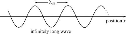
Other important hypothesis of quantum mechanics is the correspondence principle. We assume the following suitable statement: the wave-function $\Psi(\mathbf{q}, t)$ can be approximated in the quasi-classic limit $\hbar \rightarrow 0$ as follows (12):
$$
\Psi(\mathbf{q}, t) \sim \exp [i S(\mathbf{q}, t) / \hbar],
$$
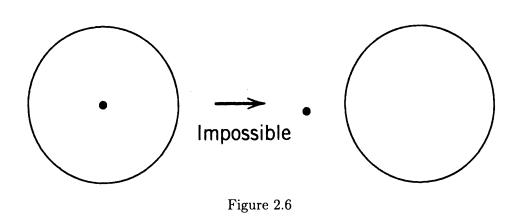
where $S(\mathbf{q}, t)$ is the classical action of the system associated with the known Hamilton-Jacobi theory of classical mechanics. Physically, this principle expresses that quantum mechanics contains classical mechanics as an asymptotic theory. At the same time, it states that quantum mechanics should be formulated under the correspondence with classical mechanics. Physically speaking, it is impossible to introduce a consistent quantum mechanics formulation without the consideration of classical notions. Precisely, this is a very consequence of the complementarity between the dynamical description performed in terms of the wave function $\Psi$ and the space-time classical description associated with the results of experimental measurements. The completeness of quantum description performed in terms of the wave function $\Psi$ demands both the presence of quantum statistical ensemble and classical objects that play the role of measuring instruments.

Historically, correspondence principle was formally introduced by Bohr in 1920 (16), although he previously made use of it as early as 1913 in developing his model of the atom (17). According to this principle, quantum description should be consistent with classical description in the limit of large quantum numbers. In the framework of Schrödinger’s wave mechanics, this principle appears as a suitable generalization of the so-called optics-mechanical analogy (18). In geometric optics, the light propagation is described in the so-called rays approximation. According to the Fermat’s principle, the ray trajectories extremize the optical length $\ell[\mathbf{q}(s)]$ :
$$
\ell[\mathbf{q}(s)]=\int_{s_{1}}^{s)} n[\mathbf{q}(s)] d s \rightarrow \delta \ell[\mathbf{q}(s)]=0,
$$
which is calculated along the curve $\mathbf{q}(s)$ with fixed extreme points $\mathbf{q}\left(s_{1}\right)-p$ and $\mathbf{q}\left(s_{2}\right)-Q$. Here, $n(\mathbf{q})$ is the refraction index of the optical medium and $d s=|d \mathbf{q}|$. Equivalently, the rays propagation can be described by Eikonal equation:
$$
|\nabla \varphi(\mathbf{q})|^{2}=k_{0}^{2} n^{2}(\mathbf{q}),
$$
where $\varphi(\mathbf{q})$ is the phase of the undulatory function $u(\mathbf{q}, t)=a(\mathbf{q}, t) \exp [-i \omega t+i \varphi(\mathbf{q})]$ in the wave optics, $k_{0}=\omega / c$ and $c$ are the modulus of the wave vector and the speed of light in vacuum, respectively. The phase $\varphi(\mathbf{q})$ allows to obtain the wave vector $\mathbf{k}(\mathbf{q})$ within the optical medium:
$$
\mathbf{k}(\mathbf{q})=\nabla \varphi(\mathbf{q}) \rightarrow k(\mathbf{q})=|\mathbf{k}(\mathbf{q})|=k_{0} n(\mathbf{q})
$$
which provides the orientation of the ray propagation:
$$
\frac{d \mathbf{q}(s)}{d s}=\frac{\mathbf{k}(\mathbf{q})}{|\mathbf{k}(\mathbf{q})|}
$$

物理代写|理论力学作业代写Theoretical Mechanics代考|Operators of physical observables and Schrödinger equation

Physical interpretation of the wave function $\Psi(\mathbf{q}, t)$ implies that the expectation value of any arbitrary function $A(\mathbf{q})$ that is defined on the space coordinates $q$ is expressed as follows:
$$
\langle A\rangle=\int|\Psi(\mathbf{q}, t)|^{2} A(\mathbf{q}) d \mathbf{q} .
$$
For calculating the expectation value of an arbitrary physical observable $O$, the previous expression should be extended to a bilinear form in term of the wave function $\Psi(\mathbf{q}, t)(19)$ :
$$
\langle O\rangle=\int \Psi^{}(\mathbf{q}, t) O(\mathbf{q}, \tilde{\mathbf{q}}, t) \Psi(\tilde{\mathbf{q}}, t) d \mathbf{q} d \tilde{\mathbf{q}}, $$ where $O(\mathbf{q}, \tilde{\mathbf{q}}, t)$ is the kernel of the physical observable $O$. As already commented, there exist some physical observables, e.g.: the momentum $\mathbf{p}$, whose determination demands repetitions of measurements in a finite region of the space sufficient for the manifestation of wave properties of the function $\Psi(\mathbf{q}, t)$. Precisely, this type of procedure involves a comparison or correlation between different points of the space $(\mathbf{q}, \tilde{\mathbf{q}})$, which is accounted for by the kernel $O(\mathbf{q}, \tilde{\mathbf{q}}, t)$. Due to the expectation value of any physical observable $O$ is a real number, the kernel $O(\mathbf{q}, \tilde{\mathbf{q}}, t)$ should obey the hermitian condition: $$ O^{}(\tilde{\mathbf{q}}, \mathbf{q}, t)=O(\mathbf{q}, \tilde{\mathbf{q}}, t)
$$
As commented before, superposition principle (5) has naturally introduced the linear algebra on a Hilbert space $\mathcal{H}$ as the mathematical apparatus of quantum mechanics. Using the decomposition of the wave function $\Psi$ into a certain basis $\left{\Psi_{\alpha}\right}$, it is possible to obtain the following expressions:
$$
\langle O\rangle=\sum_{\alpha \beta} a_{\hat{\alpha}}^{} O_{\alpha \beta} a_{\beta}, $$ where: $$ O_{\alpha \beta}=\int \Psi_{a}^{}(\mathbf{q}, t) O(\mathbf{q}, \tilde{\mathbf{q}}, t) \Psi_{\beta}(\tilde{\mathbf{q}}, t) d \tilde{\mathbf{q}} d \mathbf{q}
$$

理论力学代写

物理代写|理论力学作业代写Theoretical Mechanics代考|The correspondence principle

量子力学的另一个重要假设是对应原理。我们假设以下合适的陈述：波函数 $\Psi(\mathbf{q}, t)$ 可以近似于准经典极限 $\hbar \rightarrow 0$ 如下 (12)：
$$
\Psi(\mathbf{q}, t) \sim \exp [i S(\mathbf{q}, t) / \hbar]
$$
在哪里 $S(\mathbf{q}, t)$ 是与已知的经典力学的 Hamilton-Jacobi 理论相关的系统的经典作用。在物理上，这一原理表达了 量子力学包含作为渐近理论的经典力学。同时，它指出量子力学应该在与经典力学的对应下进行表述。从物理上 讲，如果不考虑经典概念，就不可能引入一致的量子力学公式。准确地说，这是根据波函数执行的动力学描述之间 的互补性的一个非常结果 $\Psi$ 以及与实验测量结果相关的时空经典描述。用波函数进行的量子描述的完整性 $\Psi$ 要求量 子统计系综和扮演测量仪器角色的经典物体的存在。
从历史上看，对应原理是由玻尔在 1920 年正式引入的（16），尽管他早在 1913 年就使用它来开发他的原子模型 (17) 。根据这一原理，量子描述应该与大量子数极限下的经典描述保持一致。在薛定谔的波动力学框架中，这 一原理似乎是对所胃的光学-机械类比 (18) 的适当概括。在几何光学中，光的传播是用所谓的射线近似来描述的。 根据费马原理，光线轨迹使光学长度达到极限 $\ell[\mathbf{q}(s)]$ :
$$
\ell[\mathbf{q}(s)]=\int_{s_{1}}^{s)} n[\mathbf{q}(s)] d s \rightarrow \delta \ell[\mathbf{q}(s)]=0
$$
这是沿曲线计算的 $\mathbf{q}(s)$ 具有固定的极值点 $\mathbf{q}\left(s_{1}\right)-p$ 和 $\mathbf{q}\left(s_{2}\right)-Q$. 这里， $n(\mathbf{q})$ 是光学介质的折射率，并且 $d s=|d \mathbf{q}| \cdot$ 等效地，射线传播可以用 Eikonal 方程来描述:
$$
|\nabla \varphi(\mathbf{q})|^{2}=k_{0}^{2} n^{2}(\mathbf{q})
$$
在哪里 $\varphi(\mathbf{q})$ 是波动函数的相位 $u(\mathbf{q}, t)=a(\mathbf{q}, t) \exp [-i \omega t+i \varphi(\mathbf{q})]$ 在波动光学中， $k_{0}=\omega / c$ 和 $c$ 分别是波 矢量的模量和真空中的光速。阶段 $\varphi(\mathbf{q})$ 允许获得波矢量 $\mathbf{k}(\mathbf{q})$ 光介质内:
$$
\mathbf{k}(\mathbf{q})=\nabla \varphi(\mathbf{q}) \rightarrow k(\mathbf{q})=|\mathbf{k}(\mathbf{q})|=k_{0} n(\mathbf{q})
$$
它提供了光线传播的方向:
$$
\frac{d \mathbf{q}(s)}{d s}=\frac{\mathbf{k}(\mathbf{q})}{|\mathbf{k}(\mathbf{q})|}
$$

物理代写|理论力学作业代写Theoretical Mechanics代考|Operators of physical observables and Schrödinger equation

波函数的物理解释 $\Psi(\mathbf{q}, t)$ 意味着任意函数的期望值 $A(\mathbf{q})$ 在空间坐标上定义 $q$ 表示如下:
$$
\langle A\rangle=\int|\Psi(\mathbf{q}, t)|^{2} A(\mathbf{q}) d \mathbf{q} .
$$
用于计算任意物理可观测量的期望值 $O$ ，前面的表达式应该根据波函数扩展为双线性形式 $\Psi(\mathbf{q}, t)(19)$ :
$$
\langle O\rangle=\int \Psi(\mathbf{q}, t) O(\mathbf{q}, \tilde{\mathbf{q}}, t) \Psi(\tilde{\mathbf{q}}, t) d \mathbf{q} d \tilde{\mathbf{q}}
$$
在哪里 $O(\mathbf{q}, \tilde{\mathbf{q}}, t)$ 是物理可观察的核 $O$. 如前所述，存在一些物理可观察量，例如：动量 $\mathbf{p}$ ，其确定需要在空间的 有限区域内重复测量，足以显示函数的波特性 $\Psi(\mathbf{q}, t)$. 准确地说，这种类型的过程涉及空间不同点之间的比较或 相关性 $(\mathbf{q}, \tilde{\mathbf{q}})$ ，这是由内核解释的 $O(\mathbf{q}, \tilde{\mathbf{q}}, t)$. 由于任何物理可观察的期望值 $O$ 是一个实数，内核 $O(\mathbf{q}, \tilde{\mathbf{q}}, t)$ 应服 从厄米特条件:
$$
O(\tilde{\mathbf{q}}, \mathbf{q}, t)=O(\mathbf{q}, \tilde{\mathbf{q}}, t)
$$
$\mathrm{~ 如 前 所 述 ， 喗 加 原 理 ~ ( 5 ) ~ 自 然 地 在 希 尔 伯 特 空 间 上 引 入 了 线 性 代 数}$ 解 $\Psi$ 进入一定的基础 Ueft{{Psi_{lalpha}\right }, 可以得到以下表达式:
$$
\langle O\rangle=\sum_{\alpha \beta} a_{\hat{\alpha}} O_{\alpha \beta} a_{\beta},
$$
在哪里:
$$
O_{\alpha \beta}=\int \Psi_{a}(\mathbf{q}, t) O(\mathbf{q}, \tilde{\mathbf{q}}, t) \Psi_{\beta}(\tilde{\mathbf{q}}, t) d \tilde{\mathbf{q}} d \mathbf{q}
$$

统计代写请认准statistics-lab™. statistics-lab™为您的留学生涯保驾护航。

金融工程代写

金融工程是使用数学技术来解决金融问题。金融工程使用计算机科学、统计学、经济学和应用数学领域的工具和知识来解决当前的金融问题，以及设计新的和创新的金融产品。

非参数统计代写

非参数统计指的是一种统计方法，其中不假设数据来自于由少数参数决定的规定模型；这种模型的例子包括正态分布模型和线性回归模型。

广义线性模型代考

广义线性模型（GLM）归属统计学领域，是一种应用灵活的线性回归模型。该模型允许因变量的偏差分布有除了正态分布之外的其它分布。

术语 广义线性模型（GLM）通常是指给定连续和/或分类预测因素的连续响应变量的常规线性回归模型。它包括多元线性回归，以及方差分析和方差分析（仅含固定效应）。

有限元方法代写

有限元方法（FEM）是一种流行的方法，用于数值解决工程和数学建模中出现的微分方程。典型的问题领域包括结构分析、传热、流体流动、质量运输和电磁势等传统领域。

有限元是一种通用的数值方法，用于解决两个或三个空间变量的偏微分方程（即一些边界值问题）。为了解决一个问题，有限元将一个大系统细分为更小、更简单的部分，称为有限元。这是通过在空间维度上的特定空间离散化来实现的，它是通过构建对象的网格来实现的：用于求解的数值域，它有有限数量的点。边界值问题的有限元方法表述最终导致一个代数方程组。该方法在域上对未知函数进行逼近。[1] 然后将模拟这些有限元的简单方程组合成一个更大的方程系统，以模拟整个问题。然后，有限元通过变化微积分使相关的误差函数最小化来逼近一个解决方案。

tatistics-lab作为专业的留学生服务机构，多年来已为美国、英国、加拿大、澳洲等留学热门地的学生提供专业的学术服务，包括但不限于Essay代写，Assignment代写，Dissertation代写，Report代写，小组作业代写，Proposal代写，Paper代写，Presentation代写，计算机作业代写，论文修改和润色，网课代做，exam代考等等。写作范围涵盖高中，本科，研究生等海外留学全阶段，辐射金融，经济学，会计学，审计学，管理学等全球99%专业科目。写作团队既有专业英语母语作者，也有海外名校硕博留学生，每位写作老师都拥有过硬的语言能力，专业的学科背景和学术写作经验。我们承诺100%原创，100%专业，100%准时，100%满意。

随机分析代写

随机微积分是数学的一个分支，对随机过程进行操作。它允许为随机过程的积分定义一个关于随机过程的一致的积分理论。这个领域是由日本数学家伊藤清在第二次世界大战期间创建并开始的。

时间序列分析代写

随机过程，是依赖于参数的一组随机变量的全体，参数通常是时间。 随机变量是随机现象的数量表现，其时间序列是一组按照时间发生先后顺序进行排列的数据点序列。通常一组时间序列的时间间隔为一恒定值（如1秒，5分钟，12小时，7天，1年），因此时间序列可以作为离散时间数据进行分析处理。研究时间序列数据的意义在于现实中，往往需要研究某个事物其随时间发展变化的规律。这就需要通过研究该事物过去发展的历史记录，以得到其自身发展的规律。

回归分析代写

多元回归分析渐进（Multiple Regression Analysis Asymptotics）属于计量经济学领域，主要是一种数学上的统计分析方法，可以分析复杂情况下各影响因素的数学关系，在自然科学、社会和经济学等多个领域内应用广泛。

MATLAB代写

MATLAB 是一种用于技术计算的高性能语言。它将计算、可视化和编程集成在一个易于使用的环境中，其中问题和解决方案以熟悉的数学符号表示。典型用途包括：数学和计算算法开发建模、仿真和原型制作数据分析、探索和可视化科学和工程图形应用程序开发，包括图形用户界面构建MATLAB 是一个交互式系统，其基本数据元素是一个不需要维度的数组。这使您可以解决许多技术计算问题，尤其是那些具有矩阵和向量公式的问题，而只需用 C 或 Fortran 等标量非交互式语言编写程序所需的时间的一小部分。MATLAB 名称代表矩阵实验室。MATLAB 最初的编写目的是提供对由 LINPACK 和 EISPACK 项目开发的矩阵软件的轻松访问，这两个项目共同代表了矩阵计算软件的最新技术。MATLAB 经过多年的发展，得到了许多用户的投入。在大学环境中，它是数学、工程和科学入门和高级课程的标准教学工具。在工业领域，MATLAB 是高效研究、开发和分析的首选工具。MATLAB 具有一系列称为工具箱的特定于应用程序的解决方案。对于大多数 MATLAB 用户来说非常重要，工具箱允许您学习和应用专业技术。工具箱是 MATLAB 函数（M 文件）的综合集合，可扩展 MATLAB 环境以解决特定类别的问题。可用工具箱的领域包括信号处理、控制系统、神经网络、模糊逻辑、小波、仿真等。

R语言代写	问卷设计与分析代写
PYTHON代写	回归分析与线性模型代写
MATLAB代写	方差分析与试验设计代写
STATA代写	机器学习/统计学习代写
SPSS代写	计量经济学代写
EVIEWS代写	时间序列分析代写
EXCEL代写	深度学习代写
SQL代写	各种数据建模与可视化代写

如果你也在 怎样代写理论力学Theoretical Mechanics这个学科遇到相关的难题，请随时右上角联系我们的24/7代写客服。

理论力学是研究物质的运动和导致这种运动的力量。它被应用于分析任何动态系统，从原子到太阳系。薄壁管的应力、变形和稳定性分析是物理学和工程学的一个经典课题。

statistics-lab™ 为您的留学生涯保驾护航 在代写理论力学Theoretical Mechanics方面已经树立了自己的口碑, 保证靠谱, 高质且原创的统计Statistics代写服务。我们的专家在代写理论力学Theoretical Mechanics代写方面经验极为丰富，各种代写理论力学Theoretical Mechanics相关的作业也就用不着说。

我们提供的理论力学Theoretical Mechanics及其相关学科的代写，服务范围广, 其中包括但不限于:

• Statistical Inference 统计推断
• Statistical Computing 统计计算
• Advanced Probability Theory 高等概率论
• Advanced Mathematical Statistics 高等数理统计学
• (Generalized) Linear Models 广义线性模型
• Statistical Machine Learning 统计机器学习
• Longitudinal Data Analysis 纵向数据分析
• Foundations of Data Science 数据科学基础

物理代写|理论力学作业代写Theoretical Mechanics代考|The wave function Ψ and its physical relevance

Dynamical description of a quantum system is performed in terms of the so-called the wave function $\Psi$ (12). For example, such as the frequency $\omega$ and wave vector $\mathbf{k}$ observed in electron diffraction experiments are related to dynamical variables as energy $E$ and momentum $p$ in terms of de Broglie’s relations (2). Accordingly, the wave function $\Psi(\mathbf{q}, t)$ associated with a free microparticle (as the electrons in a beam with very low intensity) behaves as follows:
$$
\Psi(\mathbf{q}, t)=C \exp [-i(E t-\mathbf{p} \cdot \mathbf{q}) / \hbar]
$$
Historically, de Broglie proposed the relations (2) as a direct generalization of quantum hypothesis of light developed by Planck and Einstein for any kind of microparticles (14). The experimental confirmation of these wave-particle duality for any kind of matter revealed the unity of material world. In fact, wave-particle duality is a property of matter as universal as the fact that any kind of matter is able to produce a gravitational interaction.

While the state of a system in classical mechanics is determined by the knowledge of the positions $\mathbf{q}$ and momenta $\mathbf{p}$ of all its constituents, the state of a system in the framework of quantum mechanics is determined by the knowledge of its wave function $\Psi(\mathbf{q}, t)$ (or its generalization $\Psi\left(\mathbf{q}^{1}, \mathbf{q}^{2}, \ldots, \mathbf{q}^{n}, t\right)$ for a system with many constituents, notation that is omitted hereafter for the sake of simplicity). In fact, the knowledge of the wave function $\Psi\left(\mathbf{q}, t_{0}\right)$ in an initial instant $t_{0}$ allows the prediction of its future evolution prior to the realization of a measurement (12). The wave function $\Psi(\mathbf{q}, t)$ is a complex function whose modulus $|\Psi(\mathbf{q}, t)|^{2}$ describes the probability density, in an absolute or relative sense, to detect a microparticle at the position $\mathrm{q}$ as a result of a measurement at the time $t$ (15). Such a statistical relevance of the wave function $\Psi(\mathbf{q}, t)$ about its relation with the experimental results is the most condensed expression of complementarity of quantum phenomena.

Due to its statistical relevance, the reconstruction of the wave function $\Psi(\mathbf{q}, t)$ from a given experimental situation demands the notion of statistical ensemble (12). In electron diffraction experiments, each electron in the beam manifests undulatory properties in its dynamical behavior. However, the interaction of this microparticle with a measuring instrument (a classical object as a photographic plate) radically affects its initial state, e.g.: electron is forced to localize in a very narrow region (the spot). In this case, a single measuring process is useless to reveal the wave properties of its previous quantum state. To rebuild the wave function $\Psi$ (up to the precision of an unimportant constant complex factor $e^{i \phi}$ ), it is necessary to perform infinite repeated measurements of the quantum system under the same initial conditions. Abstractly, this procedure is equivalent to consider simultaneous measurements over a quantum statistical ensemble: such as an infinite set of identical copies of the quantum system, which have been previously prepared under the same experimental procedure ${ }^{2}$. Due to the important role of measurements in the knowledge state of quantum systems, quantum mechanics is a physical theory that allows us to predict the results of certain experimental measurements taken over a quantum statistical ensemble that it has been previously prepared under certain experimental criteria (12).

物理代写|理论力学作业代写Theoretical Mechanics代考|The superposition principle

To explains interference phenomena observed in the double-slit experiments, the wave function $\Psi(\mathbf{q}, t)$ of a quantum system should satisfy the superposition principle (12):
$$
\Psi(\mathbf{q}, t)=\sum_{a} a_{i t} \Psi_{a t}(\mathbf{q}, t) .
$$
Here, $\Psi_{a}(\mathbf{q}, t)$ represents the normalized wave function associated with the $\alpha$-th independent state. As example, $\Psi_{a}(\mathbf{q}, t)$ could represent the wave function contribution associated with each slit during electron interference experiments; while the modulus $\left|a_{i c}\right|^{2}$ of the complex amplitudes $a_{\alpha}$ are proportional to incident beam intensities $I_{\alpha}$, or equivalently, the probability $p_{\alpha}$ that a given electron crosses through the $\alpha$-th slit.

Superposition principle is the most important hypothesis with a positive content of quantum theory. In particular, it evidences that dynamical equations of the wave function $\Psi(\mathbf{q}, t)$ should exhibit a linear character. By itself, the superposition principle allows to assume linear algebra as the mathematical apparatus of quantum mechanics. Thus, the wave function $\Psi(\mathbf{q}, t)$ can be regarded as a complex vector in a Hilbert space $\mathcal{H}$. Under this interpretation, the superposition formula (5) can be regarded as a decomposition of a vector $\Psi$ in a basis of independent vectors $\left{\Psi_{\alpha}\right}$. The normalization of the wave function $\Psi$ can be interpreted as the vectorial norm:
$$
|\Psi|^{2}=\int \Psi^{}(\mathbf{q}, t) \Psi(\mathbf{q}, t) d \mathbf{q}=\sum_{\alpha \beta} g_{\alpha \beta} a_{i}^{} a_{\beta}=1 .
$$
Here, the matrix elements $g_{\alpha \beta}$ denote the scalar product (complex) between different basis elements:
$$
g_{\alpha \beta}=\int \Psi_{\alpha}^{}(\mathbf{q}, t) \Psi_{\beta}(\mathbf{q}, t) d \mathbf{q} $$ which accounts for the existence of interference effects during the experimental measurements. As expected, the interference matrix, $g_{\alpha \beta}$, is a hermitian matrix, $g_{\alpha \beta}=g_{\beta a}^{}$. The basis $\left{\Psi_{\alpha}(\mathbf{q}, t)\right}$ is said to be orthonormal if their elements satisfy orthogonality condition:
$$
\int \Psi_{\alpha}^{}(\mathbf{q}, t) \Psi_{\beta}(\mathbf{q}, t) d \mathbf{q}=\delta_{\alpha \beta} $$ where $\delta_{\alpha \beta}$ represents Kroneker delta (for a basis with discrete elements) or a Dirac delta functions (for the basis with continuous elements). The basis of independent states is complete if any admissible state $\Psi \in \mathcal{H}$ can be represented with this basis. In particular, a basis with independent orthogonal elements is complete if it satisfies the completeness condition: $$ \sum_{\alpha} \Psi_{a}^{}(\tilde{\mathbf{q}}, t) \Psi_{\alpha}(\mathbf{q}, t)=\delta(\tilde{\mathbf{q}}-\mathbf{q})
$$

理论力学代写

物理代写|理论力学作业代写Theoretical Mechanics代考|The wave function Ψ and its physical relevance

量子系统的动态描述是根据所谓的波函数进行的 $\Psi(12)$ 。例如，如频率 $\omega$ 和波矢量 $\mathbf{k}$ 在电子衍射实验中观察到的动 态变量与能量有关 $E$ 和势头 $p$ 根据德布罗意的关系 (2)。因此，波函数 $\Psi(\mathbf{q}, t)$ 与自由微粒相关的 (作为强度非常低 的光束中的电子) 表现如下:
$$
\Psi(\mathbf{q}, t)=C \exp [-i(E t-\mathbf{p} \cdot \mathbf{q}) / \hbar]
$$
从历史上看，德布罗意提出了关系 (2) 作为普朗克和爱因斯坦为任何类型的微粒 (14) 开发的光的量子假设的直 接推广。对任何物质的波粒二象性的实验证实，揭示了物质世界的统一性。事实上，波粒二象性是物质的一种普遍 性，就像任何一种物质都能够产生引力相互作用一样。
而经典力学中系统的状态是由位置的知识决定的 $\mathbf{q}$ 和动量 $\mathbf{p}$ 在其所有组成部分中，量子力学框架中系统的状态取决 于对其波函数的了解 $\Psi(\mathbf{q}, t)$ (或其概括 $\Psi\left(\mathbf{q}^{1}, \mathbf{q}^{2}, \ldots, \mathbf{q}^{n}, t\right)$ 对于具有许多组成部分的系统，为简单起见，以 下省略符号) 。其实波函数的知识 $\Psi\left(\mathbf{q}, t_{0}\right)$ 在最初的瞬间 $t_{0}$ 允许在实现测量之前预测其末来的演变 (12)。波函数 $\Psi(\mathbf{q}, t)$ 是一个复函数，其模 $|\Psi(\mathbf{q}, t)|^{2}$ 在绝对或相对意义上描述了在该位置检测微粒的概率密度 $\mathbf{q}$ 作为当时测量 的结果 $t(15)$ 。波函数的这种统计相关性 $\Psi(\mathbf{q}, t)$ 关于它与实验结果的关系是量子现象互补性的最浓缩表达。
由于其统计相关性，波函数的重建 $\Psi(\mathbf{q}, t)$ 从给定的实验情况需要统计集成的概念 (12) 。在电子衍射实验中，光 束中的每个电子在其动力学行为中都表现出波动特性。然而，这种微粒与测量仪器 (作为照相底片的经典物体) 的 相互作用从根本上影响了它的初始状态，例如：电子被白定位在一个非常狭窄的区域 (光点)。在这种情况下，单 个测量过程无法揭示其先前量子态的波动特性。重建波函数 $\Psi$ (直到不重要的常数复因子的精度 $e^{i \phi}$ )，需要在相同 的初始条件下对量子系统进行无限重复测量。抽象地说，这个过程等效于考虑对量子统计集合的同时测量: 例如量 子系统的无限组相同副本，这些副本先前已在相同的实验程序下准备好 ${ }^{2}$. 由于测量在量子系统的知识状态中的重要 作用，量子力学是一种物理理论，它使我们能够预测对先前在某些实验标准下准备的量子统计集合进行的某些实验 测量的结果 (12) 。

物理代写|理论力学作业代写Theoretical Mechanics代考|The superposition principle

为了解释在双缝实验中观察到的干涉现象，波函数 $\Psi(\mathbf{q}, t)$ 一个量子系统应该满足敺加原理 (12)：
$$
\Psi(\mathbf{q}, t)=\sum_{a} a_{i t} \Psi_{a t}(\mathbf{q}, t) .
$$
这里， $\Psi_{a}(\mathbf{q}, t)$ 表示与相关的归一化波函数 $\alpha$-第一个独立国家。例如， $\Psi_{a}(\mathbf{q}, t)$ 可以表示在电子干涉实验中与每 个狭峰相关的波函数贡献；而模数 $\left|a_{i c}\right|^{2}$ 复振幅 $a_{\alpha}$ 与入射光束强度成正比 $I_{\alpha}$ ，或者等价地，概率 $p_{\alpha}$ 一个给定的电 子穿过 $\alpha$-th 狭峰。
叠加原理是量子理论中最重要的具有正面内容的假设。特别是，它证明了波函数的动力学方程 $\Psi(\mathbf{q}, t)$ 应该表现出 线性特征。就其本身而言，叠加原理允许将线性代数假设为量子力学的数学工具。因此，波函数 $\Psi(\mathbf{q}, t)$ 可以看作 是希尔伯特空间中的复向量 $\mathcal{H} \mathrm{~ . ~ 在 这 种 解 释 下 ， 叒}$ Veft{{Psi_{{alpha}|right}. 波函数的归一化 $\Psi$ 可以解释为向量范数：
$$
|\Psi|^{2}=\int \Psi(\mathbf{q}, t) \Psi(\mathbf{q}, t) d \mathbf{q}=\sum_{\alpha \beta} g_{\alpha \beta} a_{i} a_{\beta}=1 .
$$
这里，矩阵元素 $g_{\alpha \beta}$ 表示不同基元素之间的标量积（复数）：
$$
g_{\alpha \beta}=\int \Psi_{\alpha}(\mathbf{q}, t) \Psi_{\beta}(\mathbf{q}, t) d \mathbf{q}
$$
这说明了在实验测量过程中存在干扰效应。正如所料，干扰矩阵， $g_{\alpha \beta}$, 是厄米矩阵, $g_{\alpha \beta}=g_{\beta a}$. 基础 Uleft{{Psi_{{alpha}(Imathbf{q}, t)\right } } \text { 如果它们的元素满足正交性条件，则称它们是正交的: }
$$
\int \Psi_{\alpha}(\mathbf{q}, t) \Psi_{\beta}(\mathbf{q}, t) d \mathbf{q}=\delta_{\alpha \beta}
$$
在哪里 $\delta_{\alpha \beta}$ 表示 Kroneker delta（对于具有离散元素的基）或 Dirac delta 函数（对于具有连续元素的基）。如果 有任何可接受的状态，则独立状态的基础是完整的 $\Psi \in \mathcal{H}$ 可以用这个基础来表示。特别是，如果满足完备性条 件，则具有独立正交元素的基是完备的:
$$
\sum_{\alpha} \Psi_{a}(\tilde{\mathbf{q}}, t) \Psi_{\alpha}(\mathbf{q}, t)=\delta(\tilde{\mathbf{q}}-\mathbf{q})
$$

统计代写请认准statistics-lab™. statistics-lab™为您的留学生涯保驾护航。

金融工程代写

金融工程是使用数学技术来解决金融问题。金融工程使用计算机科学、统计学、经济学和应用数学领域的工具和知识来解决当前的金融问题，以及设计新的和创新的金融产品。

非参数统计代写

非参数统计指的是一种统计方法，其中不假设数据来自于由少数参数决定的规定模型；这种模型的例子包括正态分布模型和线性回归模型。

广义线性模型代考

广义线性模型（GLM）归属统计学领域，是一种应用灵活的线性回归模型。该模型允许因变量的偏差分布有除了正态分布之外的其它分布。

术语 广义线性模型（GLM）通常是指给定连续和/或分类预测因素的连续响应变量的常规线性回归模型。它包括多元线性回归，以及方差分析和方差分析（仅含固定效应）。

有限元方法代写

有限元方法（FEM）是一种流行的方法，用于数值解决工程和数学建模中出现的微分方程。典型的问题领域包括结构分析、传热、流体流动、质量运输和电磁势等传统领域。

有限元是一种通用的数值方法，用于解决两个或三个空间变量的偏微分方程（即一些边界值问题）。为了解决一个问题，有限元将一个大系统细分为更小、更简单的部分，称为有限元。这是通过在空间维度上的特定空间离散化来实现的，它是通过构建对象的网格来实现的：用于求解的数值域，它有有限数量的点。边界值问题的有限元方法表述最终导致一个代数方程组。该方法在域上对未知函数进行逼近。[1] 然后将模拟这些有限元的简单方程组合成一个更大的方程系统，以模拟整个问题。然后，有限元通过变化微积分使相关的误差函数最小化来逼近一个解决方案。

tatistics-lab作为专业的留学生服务机构，多年来已为美国、英国、加拿大、澳洲等留学热门地的学生提供专业的学术服务，包括但不限于Essay代写，Assignment代写，Dissertation代写，Report代写，小组作业代写，Proposal代写，Paper代写，Presentation代写，计算机作业代写，论文修改和润色，网课代做，exam代考等等。写作范围涵盖高中，本科，研究生等海外留学全阶段，辐射金融，经济学，会计学，审计学，管理学等全球99%专业科目。写作团队既有专业英语母语作者，也有海外名校硕博留学生，每位写作老师都拥有过硬的语言能力，专业的学科背景和学术写作经验。我们承诺100%原创，100%专业，100%准时，100%满意。

随机分析代写

随机微积分是数学的一个分支，对随机过程进行操作。它允许为随机过程的积分定义一个关于随机过程的一致的积分理论。这个领域是由日本数学家伊藤清在第二次世界大战期间创建并开始的。

时间序列分析代写

随机过程，是依赖于参数的一组随机变量的全体，参数通常是时间。 随机变量是随机现象的数量表现，其时间序列是一组按照时间发生先后顺序进行排列的数据点序列。通常一组时间序列的时间间隔为一恒定值（如1秒，5分钟，12小时，7天，1年），因此时间序列可以作为离散时间数据进行分析处理。研究时间序列数据的意义在于现实中，往往需要研究某个事物其随时间发展变化的规律。这就需要通过研究该事物过去发展的历史记录，以得到其自身发展的规律。

回归分析代写

多元回归分析渐进（Multiple Regression Analysis Asymptotics）属于计量经济学领域，主要是一种数学上的统计分析方法，可以分析复杂情况下各影响因素的数学关系，在自然科学、社会和经济学等多个领域内应用广泛。

MATLAB代写

MATLAB 是一种用于技术计算的高性能语言。它将计算、可视化和编程集成在一个易于使用的环境中，其中问题和解决方案以熟悉的数学符号表示。典型用途包括：数学和计算算法开发建模、仿真和原型制作数据分析、探索和可视化科学和工程图形应用程序开发，包括图形用户界面构建MATLAB 是一个交互式系统，其基本数据元素是一个不需要维度的数组。这使您可以解决许多技术计算问题，尤其是那些具有矩阵和向量公式的问题，而只需用 C 或 Fortran 等标量非交互式语言编写程序所需的时间的一小部分。MATLAB 名称代表矩阵实验室。MATLAB 最初的编写目的是提供对由 LINPACK 和 EISPACK 项目开发的矩阵软件的轻松访问，这两个项目共同代表了矩阵计算软件的最新技术。MATLAB 经过多年的发展，得到了许多用户的投入。在大学环境中，它是数学、工程和科学入门和高级课程的标准教学工具。在工业领域，MATLAB 是高效研究、开发和分析的首选工具。MATLAB 具有一系列称为工具箱的特定于应用程序的解决方案。对于大多数 MATLAB 用户来说非常重要，工具箱允许您学习和应用专业技术。工具箱是 MATLAB 函数（M 文件）的综合集合，可扩展 MATLAB 环境以解决特定类别的问题。可用工具箱的领域包括信号处理、控制系统、神经网络、模糊逻辑、小波、仿真等。

R语言代写	问卷设计与分析代写
PYTHON代写	回归分析与线性模型代写
MATLAB代写	方差分析与试验设计代写
STATA代写	机器学习/统计学习代写
SPSS代写	计量经济学代写
EVIEWS代写	时间序列分析代写
EXCEL代写	深度学习代写
SQL代写	各种数据建模与可视化代写

如果你也在 怎样代写理论力学Theoretical Mechanics这个学科遇到相关的难题，请随时右上角联系我们的24/7代写客服。

理论力学是研究物质的运动和导致这种运动的力量。它被应用于分析任何动态系统，从原子到太阳系。薄壁管的应力、变形和稳定性分析是物理学和工程学的一个经典课题。

statistics-lab™ 为您的留学生涯保驾护航 在代写理论力学Theoretical Mechanics方面已经树立了自己的口碑, 保证靠谱, 高质且原创的统计Statistics代写服务。我们的专家在代写理论力学Theoretical Mechanics代写方面经验极为丰富，各种代写理论力学Theoretical Mechanics相关的作业也就用不着说。

我们提供的理论力学Theoretical Mechanics及其相关学科的代写，服务范围广, 其中包括但不限于:

• Statistical Inference 统计推断
• Statistical Computing 统计计算
• Advanced Probability Theory 高等概率论
• Advanced Mathematical Statistics 高等数理统计学
• (Generalized) Linear Models 广义线性模型
• Statistical Machine Learning 统计机器学习
• Longitudinal Data Analysis 纵向数据分析
• Foundations of Data Science 数据科学基础

物理代写|理论力学作业代写Theoretical Mechanics代考|Complementarity in Quantum Mechanics

Roughly speaking, complementarity can be understood as the coexistence of multiple properties in the behavior of an object that seem to be contradictory. Although it is possible to switch among different descriptions of these properties, in principle, it is impossible to view them, at the same time, despite their simultaneous coexistence. Therefore, the consideration of all these contradictory properties is absolutely necessary to provide a complete characterization of the object. In physics, complementarity represents a basic principle of quantum theory proposed by Niels Bohr $(1 ; 2)$, which is closely identified with the Copenhagen interpretation. This notion refers to effects such as the so-called wave-particle duality. In an analogous perspective as the finite character of the speed of light $c$ implies the impossibility of a sharp separation between the notions of space and time, the finite character of the quantum of action $\hbar$ implies the impossibility of a sharp separation between the behavior of a quantum system and its interaction with the measuring instruments.

In the early days of quantum mechanics, Bohr understood that complementarity cannot be a unique feature of quantum theories $(3 ; 4)$. In fact, he suggested that the thermodynamical quantities of temperature $T$ and energy $E$ should be complementary in the same way as position $q$ and momentum $p$ in quantum mechanics. According to thermodynamics, the energy $E$ and the temperature $T$ can be simultaneously defined for a thermodynamic system in equilibrium. However, a complete and different viewpoint for the energy-temperature relationship is provided in the framework of classical statistical mechanics (5). Inspired on Gibbs canonical ensemble, Bohr claimed that a definite temperature $T$ can only be attributed to the system if it is submerged into a heat bath ${ }^{1}$, in which case fluctuations of energy $E$ are unavoidable. Conversely, a definite energy $E$ can only be assigned when the system is put into energetic isolation, thus excluding the simultaneous determination of its temperature $T$.
At first glance, the above reasonings are remarkably analogous to the Bohr’s arguments that support the complementary character between the coordinates $\mathrm{q}$ and momentum $\mathbf{p}$. Dimensional analysis suggests the relevance of the following uncertainty relation (6):
$$
\Delta E \Delta(1 / T) \geq k_{B},
$$
where $k_{B}$ is the Boltzmann’s constant, which can play in statistical mechanics the counterpart role of the Planck’s constant $\hbar$ in quantum mechanics. Recently (7-9), we have shown that Bohr’s arguments about the complementary character between energy and temperature, as well as the inequality of Eq.(1), are not strictly correct. However, the essential idea of Bohr is relevant enough: uncertainty relations can be present in any physical theory with a statistical formulation. In fact, the notion of complementarity is intrinsically associated with the statistical nature of a given physical theory.

物理代写|理论力学作业代写Theoretical Mechanics代考|Complementary descriptions and complementary quantities

Quantum mechanics is a theory hallmarked by the complementarity between two descriptions that are unified in classical physics $(1 ; 2)$ :

1. Space-time description: the parametrization in terms of coordinates $q$ and time $t$;
2. Dynamical description: This description in based on the applicability of the dynamical conseroation laws, where enter dynamical quantities as the energy and the momentum.
   The breakdown of classical notions as the concept of point particle trajectory $[\mathbf{q}(t), \mathbf{p}(t)]$ was clearly evidenced in Davisson and Germer experiment and other similar experiences (12). To illustrate that electrons and other microparticles undergo interference and diffraction phenomena like the ordinary waves, in Fig.1 a schematic representation of electron interference by double-slits apparatus is shown (13). According to this experience, the measurement results can only be described using classical notions compatible with its corpuscular representations, that is, in terms of the space-time description, e.g.: a spot in a photographic plate, a recoil of some movable part of the instrument, etc. Moreover, these experimental results are generally unpredictable, that is, they show an intrinsic statistical nature that is governed by the wave behavior dynamics. According to these experiments, there is no a sharp separation between the undulatory-statistical behavior of microparticles and the space-time description associated with the interaction with the measuring instruments.

Besides the existence of complementary descriptions, it is possible to talk about the notion of complementary quantities. Position $\mathbf{q}$ and momentum $\mathbf{p}$, as well as time $t$ and energy $E$, are relevant examples complementary quantities. Any experimental setup aimed to study the exchange of energy $E$ and momentum $p$ between microparticles must involve a measure in a finite region of the space-time for the definition of wave frequency $\omega$ and vector $\mathbf{k}$ entering in de Broglie’s relations (14):
$$
E=\hbar \omega \text { and } \mathbf{p}=\hbar \mathbf{k}
$$

理论力学代写

物理代写|理论力学作业代写Theoretical Mechanics代考|Complementarity in Quantum Mechanics

粗略地说，互补性可以理解为一个对象的行为中看似矛盾的多个属性并存。尽管可以在这些属性的不同描述之间切 换，但原则上，尽管它们同时共存，但不可能同时查看它们。因此，考虑所有这些矛盾的属性对于提供对象的完整 表征是绝对必要的。在物理学中，互补性代表了尼尔斯·玻尔提出的量子理论的一个基本原理 $(1 ; 2)$ ，这与哥本哈根 解释密切相关。这个概念指的是诸如所谓的波粒二象性之类的效应。从类似的角度来看，光速的有限特性 $c$ 意味着 空间和时间概念之间的明显分离是不可能的，作用量子的有限特性 $\hbar$ 这意味看量子系统的行为与其与测量仪器的相 互作用之间不可能有明显的分离。
在量子力学的早期，玻尔明白互补性不可能是量子理论的独特特征 $(3 ; 4)$. 事实上，他提出温度的热力学量 $T$ 和能 量 $E$ 应该以与位置相同的方式互补 $q$ 和势头 $p$ 在量子力学中。根据热力学，能量 $E$ 和温度 $T$ 可以同时为处于平衡状态 的热力学系统定义。然而，在经典统计力学的框架中提供了一个完整且不同的能量-温度关系观点 (5)。受到 Gibbs 正则系综的启发，玻尔声称一个确定的温度 $T$ 只有浸入热浴中才能归因于系统 ${ }^{1}$ ，在这种情况下能量波动 $E$ 是不可避 免的。反之，一定的能量 $E$ 只能在系统进入能量隔离时分配，因此不包括同时确定其温度 $T$.
乍一看，上述推理非常类似于玻尔的论点，即支持坐标之间的互补特征 $q$ 和势头 $p$. 量纲分析表明以下不确定性关系 (6) 的相关性:
$$
\Delta E \Delta(1 / T) \geq k_{B}
$$
在哪里 $k_{B}$ 是玻尔兹曼常数，在统计力学中可以起到普朗克常数的对应作用 $h$ 在量子力学中。最近 (7-9)，我们证 明了玻尔关于能量和温度互补特征的论点以及等式 (1) 的不等式并不严格正确。然而，玻尔的基本思想是足够相 关的: 不确定性关系可以存在于任何具有统计公式的物理理论中。事实上，互补性的概念本质上与给定物理理论的 统计性质相关。

物理代写|理论力学作业代写Theoretical Mechanics代考|Complementary descriptions and complementary quantities

量子力学是一种理论，其特点是经典物理学中统一的两种描述之间的互补性 $(1 ; 2)$ :

1. 时空描述: 坐标参数化 $q$ 和时间 $t$;
2. 动力学描述：这种描述基于动力学conseration law的适用性，其中输入动力学量作为能量和动量。
   作为点粒子轨迹概念的经典概念的分解 $[\mathbf{q}(t), \mathbf{p}(t)]$ 在戴维森和格默实验以及其他类似的经验中清楚地证明了 这一点 (12)。为了说明电子和其他微粒像普通波一样经历干涉和衍射现象，在图 1 中显示了双缝装置的电子 干涉示意图 (13) 。根据这一经验，测量结果只能用与其微粒表示相适应的经典概念来描述，即用时空描 述，例如：照相底片上的一个点，某些可移动部分的后坐力。此外，这些实验结果通常是不可预测的，也就 是说，它们显示出由波浪行为动力学控制的内在统计性质。根据这些实验，
   除了存在互补描述之外，还可以讨论互补量的概念。位置 $\mathbf{q}$ 和势头 $\mathbf{p}$, 以及时间 $t$ 和能量 $E$, 是相关例子的互补量。任 何旨在研究能量交换的实验装置 $E$ 和势头 $p$ 微粒之间必须涉及时空有限区域中的测量，以定义波频率 $\omega$ 和矢量 $\mathbf{k}$ 进入 德布罗意的关系 (14) :
   $$
   E=\hbar \omega \text { and } \mathbf{p}=\hbar \mathbf{k}
   $$

统计代写请认准statistics-lab™. statistics-lab™为您的留学生涯保驾护航。

金融工程代写

金融工程是使用数学技术来解决金融问题。金融工程使用计算机科学、统计学、经济学和应用数学领域的工具和知识来解决当前的金融问题，以及设计新的和创新的金融产品。

非参数统计代写

非参数统计指的是一种统计方法，其中不假设数据来自于由少数参数决定的规定模型；这种模型的例子包括正态分布模型和线性回归模型。

广义线性模型代考

广义线性模型（GLM）归属统计学领域，是一种应用灵活的线性回归模型。该模型允许因变量的偏差分布有除了正态分布之外的其它分布。

术语 广义线性模型（GLM）通常是指给定连续和/或分类预测因素的连续响应变量的常规线性回归模型。它包括多元线性回归，以及方差分析和方差分析（仅含固定效应）。

有限元方法代写

有限元方法（FEM）是一种流行的方法，用于数值解决工程和数学建模中出现的微分方程。典型的问题领域包括结构分析、传热、流体流动、质量运输和电磁势等传统领域。

有限元是一种通用的数值方法，用于解决两个或三个空间变量的偏微分方程（即一些边界值问题）。为了解决一个问题，有限元将一个大系统细分为更小、更简单的部分，称为有限元。这是通过在空间维度上的特定空间离散化来实现的，它是通过构建对象的网格来实现的：用于求解的数值域，它有有限数量的点。边界值问题的有限元方法表述最终导致一个代数方程组。该方法在域上对未知函数进行逼近。[1] 然后将模拟这些有限元的简单方程组合成一个更大的方程系统，以模拟整个问题。然后，有限元通过变化微积分使相关的误差函数最小化来逼近一个解决方案。

tatistics-lab作为专业的留学生服务机构，多年来已为美国、英国、加拿大、澳洲等留学热门地的学生提供专业的学术服务，包括但不限于Essay代写，Assignment代写，Dissertation代写，Report代写，小组作业代写，Proposal代写，Paper代写，Presentation代写，计算机作业代写，论文修改和润色，网课代做，exam代考等等。写作范围涵盖高中，本科，研究生等海外留学全阶段，辐射金融，经济学，会计学，审计学，管理学等全球99%专业科目。写作团队既有专业英语母语作者，也有海外名校硕博留学生，每位写作老师都拥有过硬的语言能力，专业的学科背景和学术写作经验。我们承诺100%原创，100%专业，100%准时，100%满意。

随机分析代写

随机微积分是数学的一个分支，对随机过程进行操作。它允许为随机过程的积分定义一个关于随机过程的一致的积分理论。这个领域是由日本数学家伊藤清在第二次世界大战期间创建并开始的。

时间序列分析代写

随机过程，是依赖于参数的一组随机变量的全体，参数通常是时间。 随机变量是随机现象的数量表现，其时间序列是一组按照时间发生先后顺序进行排列的数据点序列。通常一组时间序列的时间间隔为一恒定值（如1秒，5分钟，12小时，7天，1年），因此时间序列可以作为离散时间数据进行分析处理。研究时间序列数据的意义在于现实中，往往需要研究某个事物其随时间发展变化的规律。这就需要通过研究该事物过去发展的历史记录，以得到其自身发展的规律。

回归分析代写

多元回归分析渐进（Multiple Regression Analysis Asymptotics）属于计量经济学领域，主要是一种数学上的统计分析方法，可以分析复杂情况下各影响因素的数学关系，在自然科学、社会和经济学等多个领域内应用广泛。

MATLAB代写

MATLAB 是一种用于技术计算的高性能语言。它将计算、可视化和编程集成在一个易于使用的环境中，其中问题和解决方案以熟悉的数学符号表示。典型用途包括：数学和计算算法开发建模、仿真和原型制作数据分析、探索和可视化科学和工程图形应用程序开发，包括图形用户界面构建MATLAB 是一个交互式系统，其基本数据元素是一个不需要维度的数组。这使您可以解决许多技术计算问题，尤其是那些具有矩阵和向量公式的问题，而只需用 C 或 Fortran 等标量非交互式语言编写程序所需的时间的一小部分。MATLAB 名称代表矩阵实验室。MATLAB 最初的编写目的是提供对由 LINPACK 和 EISPACK 项目开发的矩阵软件的轻松访问，这两个项目共同代表了矩阵计算软件的最新技术。MATLAB 经过多年的发展，得到了许多用户的投入。在大学环境中，它是数学、工程和科学入门和高级课程的标准教学工具。在工业领域，MATLAB 是高效研究、开发和分析的首选工具。MATLAB 具有一系列称为工具箱的特定于应用程序的解决方案。对于大多数 MATLAB 用户来说非常重要，工具箱允许您学习和应用专业技术。工具箱是 MATLAB 函数（M 文件）的综合集合，可扩展 MATLAB 环境以解决特定类别的问题。可用工具箱的领域包括信号处理、控制系统、神经网络、模糊逻辑、小波、仿真等。

R语言代写	问卷设计与分析代写
PYTHON代写	回归分析与线性模型代写
MATLAB代写	方差分析与试验设计代写
STATA代写	机器学习/统计学习代写
SPSS代写	计量经济学代写
EVIEWS代写	时间序列分析代写
EXCEL代写	深度学习代写
SQL代写	各种数据建模与可视化代写

如果你也在 怎样代写理论力学Theoretical Mechanics这个学科遇到相关的难题，请随时右上角联系我们的24/7代写客服。

理论力学是研究物质的运动和导致这种运动的力量。它被应用于分析任何动态系统，从原子到太阳系。薄壁管的应力、变形和稳定性分析是物理学和工程学的一个经典课题。

statistics-lab™ 为您的留学生涯保驾护航 在代写理论力学Theoretical Mechanics方面已经树立了自己的口碑, 保证靠谱, 高质且原创的统计Statistics代写服务。我们的专家在代写理论力学Theoretical Mechanics代写方面经验极为丰富，各种代写理论力学Theoretical Mechanics相关的作业也就用不着说。

我们提供的理论力学Theoretical Mechanics及其相关学科的代写，服务范围广, 其中包括但不限于:

• Statistical Inference 统计推断
• Statistical Computing 统计计算
• Advanced Probability Theory 高等概率论
• Advanced Mathematical Statistics 高等数理统计学
• (Generalized) Linear Models 广义线性模型
• Statistical Machine Learning 统计机器学习
• Longitudinal Data Analysis 纵向数据分析
• Foundations of Data Science 数据科学基础

物理代写|理论力学作业代写Theoretical Mechanics代考|Velocity and Acceleration

The motion of a mass point is characterized by:
position vector: $\mathbf{r}(t)$,
velocity vector: $\quad \mathbf{v}(t)=\dot{\mathbf{r}}(t)$.
acceleration vector: $\mathbf{a}(t)=\ddot{\mathbf{r}}(t)$.
Higher time derivatives do not interest us in mechanics; very often they even fail to exist because in many realistic cases the acceleration is not a continuous function of time.

The typical task for mechanics consists of the calculation of the path line (trajectory) $\mathbf{r}(t)$ on the basis of a given acceleration $\mathbf{a}(t)=\ddot{\mathbf{r}}(t)$. For this purpose one has obviously to integrate $\mathbf{a}(t)$ twice with respect to time. After each integration an integration constant appears which remains undetermined unless we have two initial conditions at our disposal to fix these constants. In this connection let us assume that we know the velocity and the position of the mass point (particle) at a certain time $t_{0}$, i.e.
$$
\mathbf{a}(t) \text { for all } t, \mathbf{v}\left(t_{0}\right) \text {, and } \mathbf{r}\left(t_{0}\right)
$$
are given. Then the velocity of the particle is determined by
$$
\mathbf{v}(t)=\mathbf{v}\left(t_{0}\right)+\int_{t_{0}}^{t} d t^{\prime} \mathbf{a}\left(t^{\prime}\right)
$$
and the position vector by:
$$
\mathbf{r}(t)=\mathbf{r}\left(t_{0}\right)+\mathbf{v}\left(t_{0}\right)\left(t-t_{0}\right)+\int_{t_{0}}^{t}\left[\int_{t_{0}}^{t^{\prime}} d t^{\prime \prime} \mathbf{a}\left(t^{\prime \prime}\right)\right] d t^{\prime}
$$
Before we inspect these relations using simple examples we want to formulate the characteristic parameters of a mass point $\mathbf{r}(t), \mathbf{v}(t), \mathbf{a}(t)$ in different systems of coordinates.

物理代写|理论力学作业代写Theoretical Mechanics代考|Simple Examples

(a) Mass Point on a Straight Line
We can describe the motion without referring to any special system of coordinates. If $\mathbf{c}$ is a vector in the direction of the motion and $\mathbf{b}$ a vector perpendicular to it then we can write for the position vector of the mass point (Fig. 2.4):
$$
\mathbf{r}(t)=\mathbf{b}+\alpha(t) \mathbf{c}
$$
From this, the respective time derivatives give us the velocity and acceleration:
$$
\mathbf{v}(t)=\dot{\alpha}(t) \mathbf{c} ; \quad \mathbf{a}(t)=\ddot{\alpha}(t) \mathbf{c}
$$
(b) Uniform Straight-Line Motion
Therewith it is meant the most simple form of motion, namely the one without any acceleration:
$$
\mathbf{a}(t)=0 ; \quad \mathbf{v}(t)=\mathbf{v}_{0} \quad \text { for all } t
$$

The third summand in $(2.2)$ then disappears:
$$
\mathbf{r}(t)=\mathbf{r}\left(t_{0}\right)+\mathbf{v}{0}\left(t-t{0}\right) .
$$
This formally agrees with (2.26). The motion is thus carried out rectilinearly in the direction of the constant velocity vector $\mathbf{v}{0}$. It is called ‘uniform’ since the same distances are covered in equal time intervals (Fig. 2.5). (c) Uniformly Accelerated Motion Now we assume a constant acceleration $$ \mathbf{a}(t)=\mathbf{a}{0}
$$
That means in (2.2):
$$
\begin{aligned}
\int_{t_{0}}^{t}\left[\int_{t_{0}}^{t^{\prime}} d t^{\prime \prime} \mathbf{a}\left(t^{\prime \prime}\right)\right] d t^{\prime} &=\int_{t_{0}}^{t}\left[\mathbf{a}{0}\left(t^{\prime}-t{0}\right)\right] d t^{\prime}=\
&=\mathbf{a}{0}\left(\frac{t^{2}}{2}-\frac{t{0}^{2}}{2}\right)-\mathbf{a}{0} t{0}\left(t-t_{0}\right)=\
&=\frac{1}{2} \mathbf{a}{0}\left(t-t{0}\right)^{2} .
\end{aligned}
$$
We therewith get as path line:
$$
\mathbf{r}(t)=\mathbf{r}\left(t_{0}\right)+\mathbf{v}\left(t_{0}\right)\left(t-t_{0}\right)+\frac{1}{2} \mathbf{a}{0}\left(t-t{0}\right)^{2} .
$$
The velocity of the mass point increases linearly with time (Fig. 2.6):
$$
\mathbf{v}(t)=\mathbf{v}\left(t_{0}\right)+\mathbf{a}{0}\left(t-t{0}\right)
$$

物理代写|理论力学作业代写Theoretical Mechanics代考|Fundamental Laws of Dynamics

Up to now we have restricted ourselves to describe the motion of a mass point without investigating the primary cause of the motion. From now on, the latter will be the focus of our considerations. The goal is to develop procedures by which one can derive the explicit movement of the mass point from a known driving cause.

We start with a few very general remarks concerning the challenges and possibilities of every physical theory; here, however, with the special perspective on Classical Mechanics. Like any physical theory mechanics also is based on
definitions and theorems
The definitions are reasonably separated into basis definitions and following definitions:

By basis definitions we mean concepts like position, time, mass, …, which are no further commented on in the course of the theory. Following definitions are entities derived from the basis definitions such as velocity, acceleration, momentum, … Analogously we have also to dccompose the theorenīs:

Axioms are a matter of basic empirical facts which are mathematically not provable and will not be further justified within the theory. In the framework of Classical Mechanics these are ‘Newton’s axloms of motion’. By concluslons we understand the actual results of the physical theory. By use of the concept of the “mathematical proof’ they emerge out of the basis definitions and axioms which together are called the postulates of the theory.

The ‘ultimate judge’ of any physical theory is the experiment. The value of a theory is measured by the degree of agreement of its conclusions with the manifestations of nature. It is known today that Classical Mechanics is not able to correctly describe all movements and manifestations of the inanimate nature. In particular in atomic and subatomic regions modifications have become necessary. But one can regard Classical Mechanics as a self-consistent limiting case of a higher all-embracing theory, if it is finally found.

理论力学代写

物理代写|理论力学作业代写Theoretical Mechanics代考|Velocity and Acceleration

质点运动的特点是：
位置向量：r(吨)，
速度矢量：在(吨)=r˙(吨).
加速度矢量：一种(吨)=r¨(吨).
更高的时间导数使我们对力学不感兴趣。很多时候，它们甚至不存在，因为在许多实际情况下，加速度不是时间的连续函数。

力学的典型任务包括计算路径线（轨迹）r(吨)基于给定的加速度一种(吨)=r¨(吨). 为此，显然必须整合一种(吨)时间上的两倍。每次积分后，都会出现一个积分常数，除非我们有两个初始条件可供我们使用来固定这些常数，否则该积分常数仍未确定。在这方面，让我们假设我们知道质点（粒子）在某个时间的速度和位置吨0， IE

一种(吨) 对全部 吨,在(吨0)， 和 r(吨0)
给出。那么粒子的速度由下式确定

在(吨)=在(吨0)+∫吨0吨d吨′一种(吨′)
和位置向量：

r(吨)=r(吨0)+在(吨0)(吨−吨0)+∫吨0吨[∫吨0吨′d吨′′一种(吨′′)]d吨′
在我们使用简单的例子检查这些关系之前，我们想制定一个质点的特征参数r(吨),在(吨),一种(吨)在不同的坐标系中。

物理代写|理论力学作业代写Theoretical Mechanics代考|Simple Examples

(a) 直线上
的质点 我们可以在不参考任何特殊坐标系的情况下描述运动。如果C是运动方向上的向量，并且b一个垂直于它的向量，那么我们可以写出质点的位置向量（图 2.4）：

r(吨)=b+一种(吨)C
由此，各自的时间导数为我们提供了速度和加速度：

在(吨)=一种˙(吨)C;一种(吨)=一种¨(吨)C
(b) 匀速直线运动
它是指最简单的运动形式，即没有任何加速度的运动：

一种(吨)=0;在(吨)=在0 对全部 吨

第三条总括(2.2)然后消失：

r(吨)=r(吨0)+在0(吨−吨0).
这正式与（2.26）一致。运动因此在恒定速度矢量的方向上直线执行在0. 它被称为“均匀”，因为相同的距离以相同的时间间隔覆盖（图 2.5）。(c) 匀加速运动 现在我们假设一个匀加速

一种(吨)=一种0
这意味着在 (2.2) 中：

∫吨0吨[∫吨0吨′d吨′′一种(吨′′)]d吨′=∫吨0吨[一种0(吨′−吨0)]d吨′= =一种0(吨22−吨022)−一种0吨0(吨−吨0)= =12一种0(吨−吨0)2.
我们由此得到作为路径线：

r(吨)=r(吨0)+在(吨0)(吨−吨0)+12一种0(吨−吨0)2.
质点的速度随时间线性增加（图 2.6）：

在(吨)=在(吨0)+一种0(吨−吨0)

物理代写|理论力学作业代写Theoretical Mechanics代考|Fundamental Laws of Dynamics

到目前为止，我们仅限于描述质点的运动，而没有研究运动的主要原因。从现在开始，后者将是我们考虑的重点。目标是开发程序，通过该程序可以从已知的驱动原因推导出质点的显式运动。

我们从关于每一个物理理论的挑战和可能性的一些非常笼统的评论开始；然而，在这里，以对经典力学的特殊视角。像任何物理理论一样，力学也是基于
定义和定理
的定义被合理地分为基础定义和以下定义：

我们所说的基础定义是指位置、时间、质量等概念，在理论过程中没有进一步评论。以下定义是从速度、加速度、动量等基本定义派生而来的实体……类似地，我们还必须对理论进行分解：

公理是基本经验事实的问题，在数学上无法证明，也不会在理论中进一步证明。在经典力学的框架中，这些是“牛顿运动轴”。通过结论，我们了解物理理论的实际结果。通过使用“数学证明”的概念，它们从基础定义和公理中出现，这些基础定义和公理一起被称为理论的假设。

任何物理理论的“终极裁判”都是实验。一个理论的价值是通过其结论与自然现象的一致程度来衡量的。今天众所周知，古典力学无法正确描述无生命自然的所有运动和表现。特别是在原子和亚原子区域的修改已成为必要。但是，如果最终找到经典力学，则可以将其视为更高的无所不包理论的自洽极限情况。

统计代写请认准statistics-lab™. statistics-lab™为您的留学生涯保驾护航。

金融工程代写

金融工程是使用数学技术来解决金融问题。金融工程使用计算机科学、统计学、经济学和应用数学领域的工具和知识来解决当前的金融问题，以及设计新的和创新的金融产品。

非参数统计代写

非参数统计指的是一种统计方法，其中不假设数据来自于由少数参数决定的规定模型；这种模型的例子包括正态分布模型和线性回归模型。

广义线性模型代考

广义线性模型（GLM）归属统计学领域，是一种应用灵活的线性回归模型。该模型允许因变量的偏差分布有除了正态分布之外的其它分布。

术语 广义线性模型（GLM）通常是指给定连续和/或分类预测因素的连续响应变量的常规线性回归模型。它包括多元线性回归，以及方差分析和方差分析（仅含固定效应）。

有限元方法代写

有限元方法（FEM）是一种流行的方法，用于数值解决工程和数学建模中出现的微分方程。典型的问题领域包括结构分析、传热、流体流动、质量运输和电磁势等传统领域。

有限元是一种通用的数值方法，用于解决两个或三个空间变量的偏微分方程（即一些边界值问题）。为了解决一个问题，有限元将一个大系统细分为更小、更简单的部分，称为有限元。这是通过在空间维度上的特定空间离散化来实现的，它是通过构建对象的网格来实现的：用于求解的数值域，它有有限数量的点。边界值问题的有限元方法表述最终导致一个代数方程组。该方法在域上对未知函数进行逼近。[1] 然后将模拟这些有限元的简单方程组合成一个更大的方程系统，以模拟整个问题。然后，有限元通过变化微积分使相关的误差函数最小化来逼近一个解决方案。

tatistics-lab作为专业的留学生服务机构，多年来已为美国、英国、加拿大、澳洲等留学热门地的学生提供专业的学术服务，包括但不限于Essay代写，Assignment代写，Dissertation代写，Report代写，小组作业代写，Proposal代写，Paper代写，Presentation代写，计算机作业代写，论文修改和润色，网课代做，exam代考等等。写作范围涵盖高中，本科，研究生等海外留学全阶段，辐射金融，经济学，会计学，审计学，管理学等全球99%专业科目。写作团队既有专业英语母语作者，也有海外名校硕博留学生，每位写作老师都拥有过硬的语言能力，专业的学科背景和学术写作经验。我们承诺100%原创，100%专业，100%准时，100%满意。

随机分析代写

随机微积分是数学的一个分支，对随机过程进行操作。它允许为随机过程的积分定义一个关于随机过程的一致的积分理论。这个领域是由日本数学家伊藤清在第二次世界大战期间创建并开始的。

时间序列分析代写

随机过程，是依赖于参数的一组随机变量的全体，参数通常是时间。 随机变量是随机现象的数量表现，其时间序列是一组按照时间发生先后顺序进行排列的数据点序列。通常一组时间序列的时间间隔为一恒定值（如1秒，5分钟，12小时，7天，1年），因此时间序列可以作为离散时间数据进行分析处理。研究时间序列数据的意义在于现实中，往往需要研究某个事物其随时间发展变化的规律。这就需要通过研究该事物过去发展的历史记录，以得到其自身发展的规律。

回归分析代写

多元回归分析渐进（Multiple Regression Analysis Asymptotics）属于计量经济学领域，主要是一种数学上的统计分析方法，可以分析复杂情况下各影响因素的数学关系，在自然科学、社会和经济学等多个领域内应用广泛。

MATLAB代写

MATLAB 是一种用于技术计算的高性能语言。它将计算、可视化和编程集成在一个易于使用的环境中，其中问题和解决方案以熟悉的数学符号表示。典型用途包括：数学和计算算法开发建模、仿真和原型制作数据分析、探索和可视化科学和工程图形应用程序开发，包括图形用户界面构建MATLAB 是一个交互式系统，其基本数据元素是一个不需要维度的数组。这使您可以解决许多技术计算问题，尤其是那些具有矩阵和向量公式的问题，而只需用 C 或 Fortran 等标量非交互式语言编写程序所需的时间的一小部分。MATLAB 名称代表矩阵实验室。MATLAB 最初的编写目的是提供对由 LINPACK 和 EISPACK 项目开发的矩阵软件的轻松访问，这两个项目共同代表了矩阵计算软件的最新技术。MATLAB 经过多年的发展，得到了许多用户的投入。在大学环境中，它是数学、工程和科学入门和高级课程的标准教学工具。在工业领域，MATLAB 是高效研究、开发和分析的首选工具。MATLAB 具有一系列称为工具箱的特定于应用程序的解决方案。对于大多数 MATLAB 用户来说非常重要，工具箱允许您学习和应用专业技术。工具箱是 MATLAB 函数（M 文件）的综合集合，可扩展 MATLAB 环境以解决特定类别的问题。可用工具箱的领域包括信号处理、控制系统、神经网络、模糊逻辑、小波、仿真等。

R语言代写	问卷设计与分析代写
PYTHON代写	回归分析与线性模型代写
MATLAB代写	方差分析与试验设计代写
STATA代写	机器学习/统计学习代写
SPSS代写	计量经济学代写
EVIEWS代写	时间序列分析代写
EXCEL代写	深度学习代写
SQL代写	各种数据建模与可视化代写

如果你也在 怎样代写理论力学Theoretical Mechanics这个学科遇到相关的难题，请随时右上角联系我们的24/7代写客服。

理论力学是研究物质的运动和导致这种运动的力量。它被应用于分析任何动态系统，从原子到太阳系。薄壁管的应力、变形和稳定性分析是物理学和工程学的一个经典课题。

statistics-lab™ 为您的留学生涯保驾护航 在代写理论力学Theoretical Mechanics方面已经树立了自己的口碑, 保证靠谱, 高质且原创的统计Statistics代写服务。我们的专家在代写理论力学Theoretical Mechanics代写方面经验极为丰富，各种代写理论力学Theoretical Mechanics相关的作业也就用不着说。

我们提供的理论力学Theoretical Mechanics及其相关学科的代写，服务范围广, 其中包括但不限于:

• Statistical Inference 统计推断
• Statistical Computing 统计计算
• Advanced Probability Theory 高等概率论
• Advanced Mathematical Statistics 高等数理统计学
• (Generalized) Linear Models 广义线性模型
• Statistical Machine Learning 统计机器学习
• Longitudinal Data Analysis 纵向数据分析
• Foundations of Data Science 数据科学基础

物理代写|理论力学作业代写Theoretical Mechanics代考|Parametrization of Space Curves

In physics space curves are typical examples of vector-valued functions. To start with we choose in the $E_{3}$ an arbitrary but fixed origin of coordinates $\mathcal{O}$. Then the momentary position $P$ of a ‘particle’ is determined by the position vector $\mathbf{r}=\overrightarrow{0 P}$ (Fig. 1.57). By a ‘particle’ we understand a physical body of mass $m$ but with negligible extension in all directions. Later we will introduce for it the term ‘mass point’. In course of time the particle will in general change its position, i.e. $\mathbf{r}$ will change direction and magnitude. In a time-independent, complete orthonormal system (CONS) $\mathbf{e}_{i}$ the components of the position vector become normal time-

dependent functions:
$$
\mathbf{r}(t)=\sum_{j=1}^{3} x_{j}(t) \mathbf{e}{j} \equiv\left(x{1}(t), x_{2}(t), x_{3}(t)\right)
$$
This is called the trajectory or the path line of the particle.
The set of space points the particle passes through over the time define the socalled
$$
\text { space curve : }=\left{\mathbf{r}(t), t_{a} \leq t \leq t_{e}\right} \text {. }
$$
One calls (1.202) a parametrization of the space curve (1.203). The independent parameter in this case is the time $t$. Of course there also exist other possibilities of parametrization as we will see later in this section. Furthermore, it is clear that different path lines may parametrize the same space curve. For example this is already true when one and the same space curve is run through in opposite directions or in different time intervals.
Examples

1. Circular motion in the $x z$-plane
   Let the circle have the radius $R$ and let its center point be at the origin of coordinates (Fig. 1.58). Then a self-evident parametrization is via the angle $\varphi$ :
   $$
   \begin{aligned}
   &M={\varphi ; \quad 0 \leq \varphi \leq 2 \pi}, \
   &\mathbf{r}(\varphi)=R(\cos \varphi, 0, \sin \varphi)
   \end{aligned}
   $$
   Another parametrization can use, e.g., the $x$ component $x_{1}$ :
   $$
   \begin{aligned}
   &M=\left{x_{1} ; \quad-R \leq x_{1} \leq+R\right}, \
   &\mathbf{r}\left(x_{1}\right)=\left(x_{1}, 0, \pm \sqrt{R^{2}-x_{1}^{2}}\right)
   \end{aligned}
   $$
   where the plus sign holds for the upper, the minus sign for the lower half-plane.

物理代写|理论力学作业代写Theoretical Mechanics代考|Differentiation of Vector-Valued Functions

We consider a vector-valued function $\mathbf{a}(t)$ and look into the differential changes of the vector, i.e. the changes due to very small changes in time. Practically such a time interval, being determined by the measuring process, is of course always finite. Mathematically, however, an infinitely small time interval shall be considered. Furthermore, instead of time $t$ any other parameter can also be used in the following formulae. The vector-valued function $\mathbf{a}(t)$ in general has at different times (parameters) $t$ and $t+\Delta t$ different magnitudes and/or different directions. The magnitude of the difference vector
$$
\Delta \mathbf{a}=\mathbf{a}(t+\Delta t)-\mathbf{a}(t)
$$
will become smaller with decreasing time difference $\Delta t$, whereby its direction can change continuously in order to arrive for very small $\Delta t$ in the corresponding direction of the respective tangent.
Definition 1.4.2 Derivation of a Vector-Valued Function
$$
\frac{d \mathbf{a}}{d t}=\lim _{\Delta t \rightarrow 0} \frac{\mathbf{a}(t+\Delta t)-\mathbf{a}(t)}{\Delta t} .
$$
This definition clearly presumes that such a limiting vector does exist at all (Fig. 1.60). For time-derivatives sometimes one writes briefly:
$$
\dot{\mathbf{a}}(t) \equiv \frac{d \mathbf{a}}{d t}
$$

We represent $\mathbf{a}(t)$ in a time-independent basis system $\left{\mathbf{e}{i}\right}$ : $$ \mathbf{a}(t)=\sum{j} a_{j}(t) \mathbf{e}{j} . $$ Then it holds: $$ \mathbf{a}(t+\Delta t)-\mathbf{a}(t)=\sum{j}\left[a_{j}(t+\Delta t)-a_{j}(t)\right] \mathbf{e}{j} . $$ Therewith the differentiation of a vector-valued function is obviously and completely expressed in terms of derivatives of the time-dependent component functions: $$ \dot{\mathbf{a}}(t)=\frac{d \mathbf{a}}{d i}=\sum{j} \dot{a}{j}(t) \mathbf{e}{j}
$$
Correspondingly it holds also for all higher derivatives:
$$
\frac{d^{n}}{d t^{n}} \mathbf{a}(t)=\sum_{j}\left(\frac{d^{n}}{d t^{n}} a_{j}(t)\right) \mathbf{e}_{j} ; \quad n=0,1,2, \ldots
$$
Then it is not difficult to prove the following rules of differentiation
1) $\frac{d}{d t}[\mathbf{a}(t)+\mathbf{b}(t)]=\dot{\mathbf{a}}(t)+\dot{\mathbf{b}}(t)$,
2) $\frac{d}{d t}[f(t) \mathbf{a}(t)]=\dot{f}(t) \mathbf{a}(t)+f(t) \dot{\mathbf{a}}(t)$,
if $f(t)$ is a differentiable, scalar function,
3) $\frac{d}{d t}[\mathbf{a}(t) \cdot \mathbf{b}(t)]=\dot{\mathbf{a}}(t) \cdot \mathbf{b}(t)+\mathbf{a}(t) \cdot \dot{\mathbf{b}}(t)$,
4) $\frac{d}{d t}[\mathbf{a}(t) \times \mathbf{b}(t)]=\dot{\mathbf{a}}(t) \times \mathbf{b}(t)+\mathbf{a}(t) \times \dot{\mathbf{b}}(t)$.
In 4) we have to be very careful about the correct order of the factors.
Examples
a) velocity: $\mathbf{v}(t)=\dot{\mathbf{r}}(t)$
(always tangential to the path line),
acceleration: $\mathbf{a}(t)=\dot{\mathbf{v}}(t)=\ddot{\mathbf{r}}(t)$.
(1.215)

物理代写|理论力学作业代写Theoretical Mechanics代考|Arc Length

The integration of vector-valued functions can also be transferred to the corresponding integration of parameter-dependent component functions:
$$
\int_{t_{a}}^{t_{e}} \mathbf{a}(t) d t=\sum_{j=1}^{3} \mathbf{e}{j} \int{t_{a}}^{t_{e}} a_{j}(t) d t
$$
If the basis vectors are parameter-independent they can be drawn in front of the integral Thus in cuch a case nne integrates the vertor hy integrating its components in the ordinary manner. However, is should be expressly indicaled that the so defined integral of course depends on the special choice of the parameters and therefore does not at all represent a genuine curve property. During the course of this book we will meet other integrals of totally different type. However, at this stage we will make do with (1.217).

From now on, temporarily, we want to concentrate ourselves exclusively on space curves and path lines as examples of vector-valued functions. Thereby we assume for the following that the curve under consideration is ‘smooth’.

Definition 1.4.3 A space curve is denoted as smooth, if there exists at least one continuously differentiable parametrization $\mathbf{r}=\mathbf{r}(t)$ for which at no point we have:
$$
\frac{d \mathbf{r}}{d t}=0
$$
For such smooth space curves it often appears convenient to use the so-called arc length $s$ as curve parameter.

Definition 1.4.4 The arc length $s$ is the length of the space curve, measured along the curved line starting from an arbitrarily chosen initial point.

理论力学代写

物理代写|理论力学作业代写Theoretical Mechanics代考|Parametrization of Space Curves

在物理空间曲线是向量值函数的典型例子。首先，我们选择和3任意但固定的坐标原点这. 然后是瞬间位置磷“粒子”的大小由位置向量确定r=0磷→（图 1.57）。通过“粒子”，我们理解了一个物理质量体米但在各个方向上的延伸都可以忽略不计。稍后我们将为其引入术语“质点”。随着时间的推移，粒子通常会改变它的位置，即r会改变方向和幅度。在与时间无关的完全正交系统 (CONS) 中和一世位置向量的分量变为正常时间-

依赖函数：

r(吨)=∑j=13Xj(吨)和j≡(X1(吨),X2(吨),X3(吨))
这称为粒子的轨迹或路径线。
粒子随时间经过的空间点集合定义了所谓的

\text { 空间曲线 : }=\left{\mathbf{r}(t), t_{a} \leq t \leq t_{e}\right} \text {. }\text { 空间曲线 : }=\left{\mathbf{r}(t), t_{a} \leq t \leq t_{e}\right} \text {. }
有人称 (1.202) 为空间曲线 (1.203) 的参数化。这种情况下的独立参数是时间吨. 当然，我们将在本节后面看到，还存在其他参数化的可能性。此外，很明显，不同的路径线可以参数化相同的空间曲线。例如，当一条相同的空间曲线以相反的方向或不同的时间间隔穿过时，这已经是正确的了。
例子

1. 在圆周运动X和-plane
   让圆有半径R并使其中心点位于坐标原点（图 1.58）。然后一个不言而喻的参数化是通过角度披 :
   米=披;0≤披≤2圆周率, r(披)=R(因⁡披,0,罪⁡披)
   另一个参数化可以使用，例如，X零件X1:
   \begin{aligned} &M=\left{x_{1} ; \quad-R \leq x_{1} \leq+R\right}, \ &\mathbf{r}\left(x_{1}\right)=\left(x_{1}, 0, \pm \sqrt {R^{2}-x_{1}^{2}}\right) \end{对齐}\begin{aligned} &M=\left{x_{1} ; \quad-R \leq x_{1} \leq+R\right}, \ &\mathbf{r}\left(x_{1}\right)=\left(x_{1}, 0, \pm \sqrt {R^{2}-x_{1}^{2}}\right) \end{对齐}
   其中加号适用于上半平面，减号适用于下半平面。

物理代写|理论力学作业代写Theoretical Mechanics代考|Differentiation of Vector-Valued Functions

我们考虑一个向量值函数一种(吨)并查看向量的微分变化，即由于时间非常小的变化引起的变化。实际上，由测量过程确定的这种时间间隔当然总是有限的。然而，在数学上，应考虑无限小的时间间隔。此外，而不是时间吨任何其他参数也可以在以下公式中使用。向量值函数一种(吨)一般来说，在不同的时间（参数）吨和吨+Δ吨不同的幅度和/或不同的方向。差向量的大小

Δ一种=一种(吨+Δ吨)−一种(吨)
会随着时间差的减小而变小Δ吨, 从而它的方向可以连续改变以达到非常小的Δ吨在相应切线的相应方向上。
定义 1.4.2 向量值函数的推导

d一种d吨=林Δ吨→0一种(吨+Δ吨)−一种(吨)Δ吨.
这个定义清楚地假定这样一个限制向量确实存在（图 1.60）。对于时间导数，有时人们会简短地写道：

一种˙(吨)≡d一种d吨

我们代表一种(吨)在时间无关的基系统中\left{\mathbf{e}{i}\right}\left{\mathbf{e}{i}\right} :

一种(吨)=∑j一种j(吨)和j.然后它成立：

一种(吨+Δ吨)−一种(吨)=∑j[一种j(吨+Δ吨)−一种j(吨)]和j.因此，向量值函数的微分显然完全用时间相关分量函数的导数表示：

一种˙(吨)=d一种d一世=∑j一种˙j(吨)和j
相应地，它也适用于所有高级导数：

dnd吨n一种(吨)=∑j(dnd吨n一种j(吨))和j;n=0,1,2,…
那么不难证明以下微分规则
1)dd吨[一种(吨)+b(吨)]=一种˙(吨)+b˙(吨),
2) dd吨[F(吨)一种(吨)]=F˙(吨)一种(吨)+F(吨)一种˙(吨),
如果F(吨)是一个可微的标量函数，
3)dd吨[一种(吨)⋅b(吨)]=一种˙(吨)⋅b(吨)+一种(吨)⋅b˙(吨),
4) dd吨[一种(吨)×b(吨)]=一种˙(吨)×b(吨)+一种(吨)×b˙(吨).
4）我们必须非常小心因素的正确顺序。
示例
a) 速度：在(吨)=r˙(吨)
（总是与路径线相切），
加速度：一种(吨)=在˙(吨)=r¨(吨).
(1.215)

物理代写|理论力学作业代写Theoretical Mechanics代考|Arc Length

向量值函数的积分也可以转化为参数相关分量函数的相应积分：

∫吨一种吨和一种(吨)d吨=∑j=13和j∫吨一种吨和一种j(吨)d吨
如果基向量是参数无关的，它们可以画在积分前面。因此，在这种情况下，nne 以普通方式积分它的分量。然而，应该明确指出，如此定义的积分当然取决于参数的特殊选择，因此根本不代表真正的曲线特性。在本书的过程中，我们将遇到其他完全不同类型的积分。但是，在这个阶段，我们将使用 (1.217)。

从现在开始，我们暂时只专注于空间曲线和路径线作为向量值函数的示例。因此，我们假设所考虑的曲线是“平滑的”。

定义 1.4.3 如果存在至少一个连续可微参数化，则空间曲线表示为平滑的r=r(吨)我们绝对没有：

drd吨=0
对于这种光滑的空间曲线，使用所谓的弧长通常看起来很方便s作为曲线参数。

定义 1.4.4 弧长s是空间曲线的长度，从任意选择的初始点开始沿曲线测量。

统计代写请认准statistics-lab™. statistics-lab™为您的留学生涯保驾护航。

金融工程代写

金融工程是使用数学技术来解决金融问题。金融工程使用计算机科学、统计学、经济学和应用数学领域的工具和知识来解决当前的金融问题，以及设计新的和创新的金融产品。

非参数统计代写

非参数统计指的是一种统计方法，其中不假设数据来自于由少数参数决定的规定模型；这种模型的例子包括正态分布模型和线性回归模型。

广义线性模型代考

广义线性模型（GLM）归属统计学领域，是一种应用灵活的线性回归模型。该模型允许因变量的偏差分布有除了正态分布之外的其它分布。

术语 广义线性模型（GLM）通常是指给定连续和/或分类预测因素的连续响应变量的常规线性回归模型。它包括多元线性回归，以及方差分析和方差分析（仅含固定效应）。

有限元方法代写

有限元方法（FEM）是一种流行的方法，用于数值解决工程和数学建模中出现的微分方程。典型的问题领域包括结构分析、传热、流体流动、质量运输和电磁势等传统领域。

有限元是一种通用的数值方法，用于解决两个或三个空间变量的偏微分方程（即一些边界值问题）。为了解决一个问题，有限元将一个大系统细分为更小、更简单的部分，称为有限元。这是通过在空间维度上的特定空间离散化来实现的，它是通过构建对象的网格来实现的：用于求解的数值域，它有有限数量的点。边界值问题的有限元方法表述最终导致一个代数方程组。该方法在域上对未知函数进行逼近。[1] 然后将模拟这些有限元的简单方程组合成一个更大的方程系统，以模拟整个问题。然后，有限元通过变化微积分使相关的误差函数最小化来逼近一个解决方案。

tatistics-lab作为专业的留学生服务机构，多年来已为美国、英国、加拿大、澳洲等留学热门地的学生提供专业的学术服务，包括但不限于Essay代写，Assignment代写，Dissertation代写，Report代写，小组作业代写，Proposal代写，Paper代写，Presentation代写，计算机作业代写，论文修改和润色，网课代做，exam代考等等。写作范围涵盖高中，本科，研究生等海外留学全阶段，辐射金融，经济学，会计学，审计学，管理学等全球99%专业科目。写作团队既有专业英语母语作者，也有海外名校硕博留学生，每位写作老师都拥有过硬的语言能力，专业的学科背景和学术写作经验。我们承诺100%原创，100%专业，100%准时，100%满意。

随机分析代写

随机微积分是数学的一个分支，对随机过程进行操作。它允许为随机过程的积分定义一个关于随机过程的一致的积分理论。这个领域是由日本数学家伊藤清在第二次世界大战期间创建并开始的。

时间序列分析代写

随机过程，是依赖于参数的一组随机变量的全体，参数通常是时间。 随机变量是随机现象的数量表现，其时间序列是一组按照时间发生先后顺序进行排列的数据点序列。通常一组时间序列的时间间隔为一恒定值（如1秒，5分钟，12小时，7天，1年），因此时间序列可以作为离散时间数据进行分析处理。研究时间序列数据的意义在于现实中，往往需要研究某个事物其随时间发展变化的规律。这就需要通过研究该事物过去发展的历史记录，以得到其自身发展的规律。

回归分析代写

多元回归分析渐进（Multiple Regression Analysis Asymptotics）属于计量经济学领域，主要是一种数学上的统计分析方法，可以分析复杂情况下各影响因素的数学关系，在自然科学、社会和经济学等多个领域内应用广泛。

MATLAB代写

MATLAB 是一种用于技术计算的高性能语言。它将计算、可视化和编程集成在一个易于使用的环境中，其中问题和解决方案以熟悉的数学符号表示。典型用途包括：数学和计算算法开发建模、仿真和原型制作数据分析、探索和可视化科学和工程图形应用程序开发，包括图形用户界面构建MATLAB 是一个交互式系统，其基本数据元素是一个不需要维度的数组。这使您可以解决许多技术计算问题，尤其是那些具有矩阵和向量公式的问题，而只需用 C 或 Fortran 等标量非交互式语言编写程序所需的时间的一小部分。MATLAB 名称代表矩阵实验室。MATLAB 最初的编写目的是提供对由 LINPACK 和 EISPACK 项目开发的矩阵软件的轻松访问，这两个项目共同代表了矩阵计算软件的最新技术。MATLAB 经过多年的发展，得到了许多用户的投入。在大学环境中，它是数学、工程和科学入门和高级课程的标准教学工具。在工业领域，MATLAB 是高效研究、开发和分析的首选工具。MATLAB 具有一系列称为工具箱的特定于应用程序的解决方案。对于大多数 MATLAB 用户来说非常重要，工具箱允许您学习和应用专业技术。工具箱是 MATLAB 函数（M 文件）的综合集合，可扩展 MATLAB 环境以解决特定类别的问题。可用工具箱的领域包括信号处理、控制系统、神经网络、模糊逻辑、小波、仿真等。

R语言代写	问卷设计与分析代写
PYTHON代写	回归分析与线性模型代写
MATLAB代写	方差分析与试验设计代写
STATA代写	机器学习/统计学习代写
SPSS代写	计量经济学代写
EVIEWS代写	时间序列分析代写
EXCEL代写	深度学习代写
SQL代写	各种数据建模与可视化代写

如果你也在 怎样代写理论力学Theoretical Mechanics这个学科遇到相关的难题，请随时右上角联系我们的24/7代写客服。

理论力学是研究物质的运动和导致这种运动的力量。它被应用于分析任何动态系统，从原子到太阳系。薄壁管的应力、变形和稳定性分析是物理学和工程学的一个经典课题。

statistics-lab™ 为您的留学生涯保驾护航 在代写理论力学Theoretical Mechanics方面已经树立了自己的口碑, 保证靠谱, 高质且原创的统计Statistics代写服务。我们的专家在代写理论力学Theoretical Mechanics代写方面经验极为丰富，各种代写理论力学Theoretical Mechanics相关的作业也就用不着说。

我们提供的理论力学Theoretical Mechanics及其相关学科的代写，服务范围广, 其中包括但不限于:

• Statistical Inference 统计推断
• Statistical Computing 统计计算
• Advanced Probability Theory 高等概率论
• Advanced Mathematical Statistics 高等数理统计学
• (Generalized) Linear Models 广义线性模型
• Statistical Machine Learning 统计机器学习
• Longitudinal Data Analysis 纵向数据分析
• Foundations of Data Science 数据科学基础

物理代写|理论力学作业代写Theoretical Mechanics代考|Elementary Mathematical Operations

Two vectors $\mathbf{a}$ and $\mathbf{b}$ are added by a parallel translation of one of the vectors, say $\mathbf{b}$, such that the base point of $\mathbf{b}$ coincides with the arrowhead of the other vector a (Fig. 1.36). The sum vector $(\mathbf{a}+\mathbf{b})$ then starts at the base point of $\mathbf{a}$ and goes to the arrowhead of $\mathbf{b}$. One recognizes that $(\mathbf{a}+\mathbf{b})$ corresponds to the diagonal of the parallelogram spanned by $\mathbf{a}$ and $\mathbf{b}$ (parallelogram law). We list up some obvious rules for vector sums:
$(\alpha)$ Commutativity
$$
\mathbf{a}+\mathbf{b}=\mathbf{b}+\mathbf{a}
$$
This follows directly from the definition of the sum vector and becomes immediately clear with Fig. 1.37. Decisive for the commutativity is the free parallel mobility of the vectors in the plane.
( $\boldsymbol{\beta}$ ) Associativity
$$
(\mathbf{a}+\mathbf{b})+\mathbf{c}=\mathbf{a}+(\mathbf{b}+\mathbf{c})
$$

The validity of (1.130) can easily be read off from Fig. 1.38.
( $\gamma$ ) Vector Subtraction
$$
\mathbf{a}-\mathbf{b}=\mathbf{a}+(-\mathbf{b})
$$
Subtracting a from itself yields the so-called
$$
\text { zero (null) vector: } \quad 0=a-a
$$
the only vector which has no definite direction (Fig. 1.39). For all vectors holds:
$$
\mathbf{a}+\mathbf{0}=\mathbf{a}
$$
Because of (1.129), (1.130), (1.132) and (1.133) the set of all position vectors build a (commutative) group.
(b) Multiplication by a (Real) Number
Let $\alpha$ be a real number $(\alpha \in \mathbb{R})$ and $\mathbf{a}$ be an arbitrary vector.

物理代写|理论力学作业代写Theoretical Mechanics代考|Scalar Product

As scalar (inner, dot) product of two vectors $\mathbf{a}$ and $\mathbf{b}$ is denoted by the following number (scalar):
$$
(\mathbf{a}, \mathbf{b}) \equiv \mathbf{a} \cdot \mathbf{b}=a b \cos \vartheta, \quad \vartheta=\varangle(\mathbf{a}, \mathbf{b})
$$
Illustratively, it is the product of the length of the second vector with the projection of the first vector on the direction of the second (see Fig. 1.41).
$$
\begin{gathered}
\mathbf{a} \cdot \mathbf{b}=0, \text { if 1) } a=0 \text { or/and } b=0 \
\text { or 2) } \vartheta=\pi / 2 .
\end{gathered}
$$

$\mathbf{a}$ and $\mathbf{b}$ are orthogonal $(\mathbf{a} \perp \mathbf{b})$ if
$$
\mathbf{a} \cdot \mathbf{b}=0 \quad \text { with } a \neq 0 \text { and } b \neq 0 .
$$
Properties
(a) Commutativity
$$
\mathbf{a} \cdot \mathbf{b}=\mathbf{b} \cdot \mathbf{a}
$$
This relation is directly perceptible from the definition of the scalar product.
(b) Distributivity
$$
(\mathbf{a}+\mathbf{b}) \cdot \mathbf{c}=\mathbf{a} \cdot \mathbf{c}+\mathbf{b} \cdot \mathbf{c}
$$
Figure $1.42$ gives immediately the proof, which again exploits the free relocatability of the vectors in the plane.
(c) Bilinearity (Homogeneity)
For each real number $\alpha$ holds:
$$
(\alpha \mathbf{a}) \cdot \mathbf{b}=\mathbf{a} \cdot(\alpha \mathbf{b})=\alpha(\mathbf{a} \cdot \mathbf{b})
$$
Proof (Fig. 1.43)
$$
\begin{aligned}
\alpha>0: \quad(\alpha \mathbf{a}) \cdot \mathbf{b} &=\alpha a b \cos \vartheta \
\mathbf{a} \cdot \mathbf{b} &=a b \cos \vartheta
\end{aligned}
$$

物理代写|理论力学作业代写Theoretical Mechanics代考|Vector (Outer, Cross) Product

The product discussed in the last section assigns a number, i.e. a scalar, to the product of two vectors of a vector space. However, there exists a second type of product which addresses to two vectors a third vector from the same vector space. This is known as vector product, outer product, or cross product
$$
\mathbf{c}=\mathbf{a} \times \mathbf{b}
$$
This vector has the following properties:
$1 .$
$$
c=a b \sin \theta ; \quad \vartheta=\varepsilon(\mathbf{a}, \mathbf{b})
$$
The magnitude $c$ of the resulting vector corresponds to the area of the parallelogram spanned by the vectors $\mathbf{a}$ and $\mathbf{b}$ (Fig. 1.45).

2. $\mathbf{c}$ is oriented perpendicular to the area defined by $\mathbf{a}$ and $\mathbf{b}$ in such a way that $\mathbf{a}, \mathbf{b}$, $\mathbf{c}$ in this sequence build a right-handed coordinate system.

The second point indicates that the vector product does not simply characterize a direction but more a ‘direction of rotation, rotation sense’. Thus, in various respects the properties of a vector product are different from those of a ‘ordinary’ (polar) vector. $\mathbf{c}$ is a so-called axial vector (pseudovector). The strict distinction becomes clear with the term
Space Inversion
Reflection of all space points $\left(E_{3}\right)$ with respect to a fixed, given point, e.g. the origin of coordinates.

Polar vectors change their signs by inversion (see Fig. 1.46). On the other hand, since the rotation sense does not change after inversion, the axial vector will not change its sign (see Fig. 1.47).

We add a remark. It is clear that the scalar product of either only polar vectors or only axial vectors does not change its sign with inversion, being therefore a genuine scalar. The scalar product of a polar and an axial vector, however, changes into its negative and is for this reason called a pseudoscalar.

One has to bear in mind that the scalar product (Sect. 1.3.2) is defined between vectors of an arbitrary-dimensional vector space, while the vector product holds only for three-dimensional vectors.

理论力学代写

物理代写|理论力学作业代写Theoretical Mechanics代考|Elementary Mathematical Operations

两个向量一种和b通过其中一个向量的平行平移相加，比如说b, 使得基点b与另一个向量 a 的箭头一致（图 1.36）。和向量(一种+b)然后从基点开始一种并走向箭头b. 一个人认识到(一种+b)对应于跨越的平行四边形的对角线一种和b（平行四边形定律）。我们列出了向量和的一些明显规则：
(一种)交换性

一种+b=b+一种
这直接来自和向量的定义，并在图 1.37 中立即变得清晰。对交换性起决定性作用的是平面中向量的自由平行移动性。
(b) 关联性

(一种+b)+C=一种+(b+C)

(1.130) 的有效性可以很容易地从图 1.38 中读出。
(C) 向量减法

一种−b=一种+(−b)
从自身中减去 a 会产生所谓的

 零（空）向量： 0=一种−一种
唯一没有明确方向的向量（图 1.39）。对于所有向量成立：

一种+0=一种
由于 (1.129)、(1.130)、(1.132) 和 (1.133)，所有位置向量的集合构建了一个（可交换的）群。
(b) 乘以一个（实数）数
Let一种是一个实数(一种∈R)和一种是任意向量。

物理代写|理论力学作业代写Theoretical Mechanics代考|Scalar Product

作为两个向量的标量（内部，点）积一种和b由以下数字（标量）表示：

(一种,b)≡一种⋅b=一种b因⁡ϑ,ϑ=\变量(一种,b)
举例来说，它是第二个向量的长度与第一个向量在第二个方向上的投影的乘积（见图 1.41）。

一种⋅b=0, 如果 1) 一种=0 或/和 b=0  或 2) ϑ=圆周率/2.

一种和b是正交的(一种⊥b)如果

一种⋅b=0 和 一种≠0 和 b≠0.
性质
(a) 交换性

一种⋅b=b⋅一种
这种关系可以从标量积的定义中直接看出。
(b) 分配性

(一种+b)⋅C=一种⋅C+b⋅C
数字1.42立即给出了证明，它再次利用了平面中向量的自由重定位性。
(c) 双线性（同质性）
对于每个实数一种持有：

(一种一种)⋅b=一种⋅(一种b)=一种(一种⋅b)
证明（图 1.43）

一种>0:(一种一种)⋅b=一种一种b因⁡ϑ 一种⋅b=一种b因⁡ϑ

物理代写|理论力学作业代写Theoretical Mechanics代考|Vector (Outer, Cross) Product

上一节讨论的乘积将一个数字（即标量）分配给向量空间的两个向量的乘积。但是，存在第二种类型的乘积，它将来自同一向量空间的第三个向量寻址到两个向量。这称为向量积、外积或叉积

C=一种×b
该向量具有以下属性：
1.

C=一种b罪⁡θ;ϑ=e(一种,b)
幅度C结果向量的 对应于向量所跨越的平行四边形的面积一种和b（图 1.45）。

2. C垂直于由定义的区域定向一种和b以这样的方式一种,b, C在这个序列中建立一个右手坐标系。

第二点表明，矢量积并不是简单地表征一个方向，而是一个“旋转方向，旋转感”。因此，在各个方面，向量积的特性与“普通”（极坐标）向量的特性不同。C是所谓的轴向矢量（pseudovector）。
严格的区别在所有空间点的空间反转
反射术语中变得清晰(和3)相对于一个固定的给定点，例如坐标原点。

极向量通过反转来改变它们的符号（见图 1.46）。另一方面，由于反演后旋转方向不变，轴向矢量不会改变其符号（见图1.47）。

我们添加一个注释。很明显，仅极向量或仅轴向向量的标量积不会随着反转而改变其符号，因此是真正的标量。然而，极坐标和轴向矢量的标量积变为负值，因此称为伪标量。

必须记住，标量积（第 1.3.2 节）是在任意维向量空间的向量之间定义的，而向量积仅适用于三维向量。

统计代写请认准statistics-lab™. statistics-lab™为您的留学生涯保驾护航。

金融工程代写

金融工程是使用数学技术来解决金融问题。金融工程使用计算机科学、统计学、经济学和应用数学领域的工具和知识来解决当前的金融问题，以及设计新的和创新的金融产品。

非参数统计代写

非参数统计指的是一种统计方法，其中不假设数据来自于由少数参数决定的规定模型；这种模型的例子包括正态分布模型和线性回归模型。

广义线性模型代考

广义线性模型（GLM）归属统计学领域，是一种应用灵活的线性回归模型。该模型允许因变量的偏差分布有除了正态分布之外的其它分布。

术语 广义线性模型（GLM）通常是指给定连续和/或分类预测因素的连续响应变量的常规线性回归模型。它包括多元线性回归，以及方差分析和方差分析（仅含固定效应）。

有限元方法代写

有限元方法（FEM）是一种流行的方法，用于数值解决工程和数学建模中出现的微分方程。典型的问题领域包括结构分析、传热、流体流动、质量运输和电磁势等传统领域。

有限元是一种通用的数值方法，用于解决两个或三个空间变量的偏微分方程（即一些边界值问题）。为了解决一个问题，有限元将一个大系统细分为更小、更简单的部分，称为有限元。这是通过在空间维度上的特定空间离散化来实现的，它是通过构建对象的网格来实现的：用于求解的数值域，它有有限数量的点。边界值问题的有限元方法表述最终导致一个代数方程组。该方法在域上对未知函数进行逼近。[1] 然后将模拟这些有限元的简单方程组合成一个更大的方程系统，以模拟整个问题。然后，有限元通过变化微积分使相关的误差函数最小化来逼近一个解决方案。

tatistics-lab作为专业的留学生服务机构，多年来已为美国、英国、加拿大、澳洲等留学热门地的学生提供专业的学术服务，包括但不限于Essay代写，Assignment代写，Dissertation代写，Report代写，小组作业代写，Proposal代写，Paper代写，Presentation代写，计算机作业代写，论文修改和润色，网课代做，exam代考等等。写作范围涵盖高中，本科，研究生等海外留学全阶段，辐射金融，经济学，会计学，审计学，管理学等全球99%专业科目。写作团队既有专业英语母语作者，也有海外名校硕博留学生，每位写作老师都拥有过硬的语言能力，专业的学科背景和学术写作经验。我们承诺100%原创，100%专业，100%准时，100%满意。

随机分析代写

随机微积分是数学的一个分支，对随机过程进行操作。它允许为随机过程的积分定义一个关于随机过程的一致的积分理论。这个领域是由日本数学家伊藤清在第二次世界大战期间创建并开始的。

时间序列分析代写

随机过程，是依赖于参数的一组随机变量的全体，参数通常是时间。 随机变量是随机现象的数量表现，其时间序列是一组按照时间发生先后顺序进行排列的数据点序列。通常一组时间序列的时间间隔为一恒定值（如1秒，5分钟，12小时，7天，1年），因此时间序列可以作为离散时间数据进行分析处理。研究时间序列数据的意义在于现实中，往往需要研究某个事物其随时间发展变化的规律。这就需要通过研究该事物过去发展的历史记录，以得到其自身发展的规律。

回归分析代写

多元回归分析渐进（Multiple Regression Analysis Asymptotics）属于计量经济学领域，主要是一种数学上的统计分析方法，可以分析复杂情况下各影响因素的数学关系，在自然科学、社会和经济学等多个领域内应用广泛。

MATLAB代写

MATLAB 是一种用于技术计算的高性能语言。它将计算、可视化和编程集成在一个易于使用的环境中，其中问题和解决方案以熟悉的数学符号表示。典型用途包括：数学和计算算法开发建模、仿真和原型制作数据分析、探索和可视化科学和工程图形应用程序开发，包括图形用户界面构建MATLAB 是一个交互式系统，其基本数据元素是一个不需要维度的数组。这使您可以解决许多技术计算问题，尤其是那些具有矩阵和向量公式的问题，而只需用 C 或 Fortran 等标量非交互式语言编写程序所需的时间的一小部分。MATLAB 名称代表矩阵实验室。MATLAB 最初的编写目的是提供对由 LINPACK 和 EISPACK 项目开发的矩阵软件的轻松访问，这两个项目共同代表了矩阵计算软件的最新技术。MATLAB 经过多年的发展，得到了许多用户的投入。在大学环境中，它是数学、工程和科学入门和高级课程的标准教学工具。在工业领域，MATLAB 是高效研究、开发和分析的首选工具。MATLAB 具有一系列称为工具箱的特定于应用程序的解决方案。对于大多数 MATLAB 用户来说非常重要，工具箱允许您学习和应用专业技术。工具箱是 MATLAB 函数（M 文件）的综合集合，可扩展 MATLAB 环境以解决特定类别的问题。可用工具箱的领域包括信号处理、控制系统、神经网络、模糊逻辑、小波、仿真等。

R语言代写	问卷设计与分析代写
PYTHON代写	回归分析与线性模型代写
MATLAB代写	方差分析与试验设计代写
STATA代写	机器学习/统计学习代写
SPSS代写	计量经济学代写
EVIEWS代写	时间序列分析代写
EXCEL代写	深度学习代写
SQL代写	各种数据建模与可视化代写

如果你也在 怎样代写理论力学Theoretical Mechanics这个学科遇到相关的难题，请随时右上角联系我们的24/7代写客服。

理论力学是研究物质的运动和导致这种运动的力量。它被应用于分析任何动态系统，从原子到太阳系。薄壁管的应力、变形和稳定性分析是物理学和工程学的一个经典课题。

statistics-lab™ 为您的留学生涯保驾护航 在代写理论力学Theoretical Mechanics方面已经树立了自己的口碑, 保证靠谱, 高质且原创的统计Statistics代写服务。我们的专家在代写理论力学Theoretical Mechanics代写方面经验极为丰富，各种代写理论力学Theoretical Mechanics相关的作业也就用不着说。

我们提供的理论力学Theoretical Mechanics及其相关学科的代写，服务范围广, 其中包括但不限于:

• Statistical Inference 统计推断
• Statistical Computing 统计计算
• Advanced Probability Theory 高等概率论
• Advanced Mathematical Statistics 高等数理统计学
• (Generalized) Linear Models 广义线性模型
• Statistical Machine Learning 统计机器学习
• Longitudinal Data Analysis 纵向数据分析
• Foundations of Data Science 数据科学基础

物理代写|理论力学作业代写Theoretical Mechanics代考|Notions

The technique of ‘differentiation’, which we discussed in the previous section, follows the scope of work:
given: $\quad y=f(x)$
finding: $\quad f^{\prime}(x)=\frac{d f}{d x}:$ ‘derivation’,
The reverse program, namely
given: $\quad f^{\prime}(x)=\frac{d f}{d x}$
finding: $\quad y=f(x)$
leads to the technique of ‘integration’. Consider for example
$$
f^{\prime}(x)=c=\text { const }
$$
then we remember according to (1.77) that
$$
y=f(x)=c \cdot x
$$
fulfills the condition $f^{\prime}(x)=c$.
Definition $F(x)$ is the ‘antiderivative (primitive function)’ of $f(x)$, if it holds:
$$
F^{\prime}(x)=f(x) \quad \forall x
$$
In this connection the above example means:
$$
f(x) \equiv c \quad \curvearrowright \quad F(x)=c \cdot x+d .
$$

Because of the constant $d$ the result comes out as a full family of curves. Fixing $d$ needs the introduction of ‘boundary conditions’. We accept that:
‘Integration’ : Searching for the antiderivative (primitive function)
To generate a graphic image, the integral can be interpreted as the area under the curve $y=f(x)$. If the curve $y=f(x)$ is given then we ask ourselves how we can determine the area $F$ in Fig. $1.18$ under the curve between the limits $x=$ $a$ and $x=b$. This can easily be done for the special case that $f(x)$ represents a straight line. However, how can we calculate the area under an arbitrary (continuous) function $f(x)$ ?

In a first step, we approach the calculation of the area by decomposing the interval $[a, b]$ in $n$ equal sub-intervals $\Delta x_{n}$,
$$
\Delta x_{n}=\frac{b-a}{n} \quad n \in \mathbb{N} / 0
$$
where $x_{i}$ is the center of the $i$-th partial interval:
$$
x_{i}=a+\left(i-\frac{1}{2}\right) \Delta x_{n} ; i=1,2 \ldots, n
$$
Then $f\left(x_{i}\right) \Delta x_{n}$ is the area of the $i$-th pillar in Fig. 1.19. Hence it holds approximately for the area $F$ :
$$
F \approx \sum_{i=1}^{n} f\left(x_{i}\right) \Delta x_{n}
$$

物理代写|理论力学作业代写Theoretical Mechanics代考|First Rules of Integration

Some important rules follow directly from the definition of the integral:

• Identical bounds of integration:
  $$
  \int_{a}^{a} f(x) d x=0
  $$
• The ‘area’ in the sense of an integral has a sign because of $f(x)<^{\geq}$! For the example in Fig. $1.20$ one recognizes: $$ \begin{aligned} &F_{1}=\int_{a}^{x_{1}} f(x) d x>0 \
  &F_{2}=\int_{x_{1}}^{x_{2}} f(x) d x<0 \\ &F_{3}=\int_{x_{2}}^{x_{3}} f(x) d x>0
  \end{aligned}
  $$Constant factor $c \in \mathbb{R}$ :
• $$
• \int_{a}^{b} c \cdot f(x) d x=\lim {n \rightarrow \infty} \sum{i=1}^{n} c \cdot f\left(x_{i}\right) \Delta x_{n}=c \cdot \lim {n \rightarrow \infty} \sum{i=1}^{n} f\left(x_{i}\right) \Delta x_{n}
• $$
• Hence it holds:
• $$
• \int_{a}^{b} c \cdot f(x) d x=c \cdot \int_{a}^{b} f(x) d x
• $$
• Sum:
• Assume
• $$
• f(x) \equiv g(x)+h(x)
• $$
• then it follows from the definition of the Riemann integral:
• $$
• \begin{aligned}
• \int_{a}^{b} f(x) d x &=\lim {n \rightarrow \infty} \sum{i=1}^{n}\left(g\left(x_{i}\right)+h\left(x_{i}\right)\right) \Delta x_{n} \
• &=\lim {n \rightarrow \infty} \sum{i=1}^{n} g\left(x_{i}\right) \Delta x_{n}+\lim {n \rightarrow \infty} \sum{i=1}^{n} h\left(x_{i}\right) \Delta x_{n}
• \end{aligned}
• $$
• That means:
• $$
• \int_{a}^{b} f(x) d x=\int_{a}^{b} g(x) d x+\int_{a}^{b} h(x) d x
• $$
• The last two rules of integration (1.112) and (1.113) demonstrate the linearity of the integral.
• Partitioning the interval of integration:
• $$
• \Delta x_{n}=\frac{b-a}{n}=\Delta x_{n}^{(1)}+\Delta x_{n}^{(2)}=\frac{x_{0}-a}{n}+\frac{b-x_{0}}{n}
• $$
• Therewith we can write:
• $$
• \int_{a}^{b} f(x) d x=\lim {n \rightarrow \infty} \sum{i=1}^{n} f\left(x_{i}^{(1)}\right) \Delta x_{n}^{(1)}+\lim {n \rightarrow \infty} \sum{i=1}^{n} f\left(x_{i}^{(2)}\right) \Delta x_{n}^{(2)}
• $$

物理代写|理论力学作业代写Theoretical Mechanics代考|Fundamental Theorem of Calculus

We consider the definite integral over a continuous function $f(t)$, but now with variable upper limit:
$$
F(x)=\int_{a}^{x} f(t) d t
$$
‘area function’

The area under the curve $f(t)$ in this case is not constant but a function of $x$ (Fig. 1.22). If the upper bound of integration is shifted by $\Delta x$ the area will change by:
$$
\Delta F=F(x+\Delta x)-F(x)=\int_{a}^{x+\Delta x} f(t) d t-\int_{a}^{x} f(t) d t=\int_{x}^{x+\Delta x} f(t) d t
$$
In the last step we have used the rule (1.114). Without explicit proof we accept the important
‘mean value theorem of integral calculus’
This theorem implies:
$$
\exists \hat{x} \in[x, x+\Delta x] \text { with } \Delta F=\Delta x \cdot f(\hat{x}) \text {. }
$$
Although not exactly proven the theorem appears rather plausible according to Fig. 1.23. So we can further conclude:
$$
F^{\prime}(x)=\lim {\Delta x \rightarrow 0} \frac{\Delta F}{\Delta x}=\lim {\Delta x \rightarrow 0} f(\hat{x})=f(x)
$$
Thus after $(1.105)$, the area function is the antiderivative of $f(x)$ ! Furthermore, the equivalence of the definitions $(1.105)$ and $(1.110)$ for the antiderivative, which

remained unsettled in Sect. 1.2.1, is now settled.
‘fundamental theorem of calculus’
$$
\frac{d}{d x} F(x) \equiv \frac{d}{d x} \int_{a}^{x} f(t) d t=f(x) .
$$
The successive performing of integration and differentiation obviously cancel each other!
$$
\text { integration } \cong \text { inversion of differentiation }
$$
The influence of the lower limit of integration in (1.118) still appears unsettled (Fig. 1.24). To clarify this we therefore investigate:
$$
\tilde{F}(x)=\int_{a^{\prime}}^{x} f(t) d t=\underbrace{\int_{a^{\prime}}^{a} f(t) d t}{=A, \text { independent of } x}+\underbrace{\int{a}^{x} f(t) d t}_{F(x)} .
$$
Therewith it follows that both $F(x)$ and $\tilde{F}(x)$ are antiderivatives of $f(x)$ :
$$
\tilde{F}(x)=F(x)+A \curvearrowright \frac{d}{d x} \tilde{F}(x)=\frac{d}{d x} F(x)=f(x) .
$$
The lower limit of integration is therefore in a certain sense dummy, the antiderivative is uniquely fixed except for an additive constant:
$$
F(x) \Longleftrightarrow \tilde{F}(x)=F(x)+A .
$$
Therefore one introduces the
$$
\text { ‘indefinite integral’: } \quad F(x)=\int f(x) d x \text {. }
$$
defining therewith the set of all antiderivatives of $f(x)$ !

理论力学代写

物理代写|理论力学作业代写Theoretical Mechanics代考|Notions

我们在上一节中讨论的“微分”技术遵循工作范围：
给定：是=F(X)
发现：F′(X)=dFdX:’derivation’，
逆向程序，即
给出：F′(X)=dFdX
发现：是=F(X)
导致“整合”技术。考虑例如

F′(X)=C= 常量 
然后我们记得根据（1.77）

是=F(X)=C⋅X
满足条件F′(X)=C.
定义F(X)是’反导数（原始函数）’F(X)，如果它成立：

F′(X)=F(X)∀X
在这方面，上面的例子意味着：

F(X)≡C↷F(X)=C⋅X+d.

因为不断d结果是一个完整的曲线族。定影d需要引入“边界条件”。我们接受：
“积分”：搜索反导数（原始函数）
要生成图形图像，积分可以解释为曲线下的面积是=F(X). 如果曲线是=F(X)给出然后我们问自己我们如何确定该区域F在图。1.18在界限之间的曲线下X= 一种和X=b. 对于以下特殊情况，这可以很容易地完成F(X)代表一条直线。但是，我们如何计算任意（连续）函数下的面积F(X) ?

第一步，我们通过分解区间来计算面积[一种,b]在n相等的子区间ΔXn,

ΔXn=b−一种nn∈ñ/0
在哪里X一世是中心一世-第部分间隔：

X一世=一种+(一世−12)ΔXn;一世=1,2…,n
然后F(X一世)ΔXn是面积一世-图 1.19 中的第一个支柱。因此，它大约适用于该地区F :

F≈∑一世=1nF(X一世)ΔXn

物理代写|理论力学作业代写Theoretical Mechanics代考|First Rules of Integration

一些重要的规则直接来自积分的定义：

• 相同的积分界限：
  ∫一种一种F(X)dX=0
• 积分意义上的“面积”有一个符号，因为F(X)<≥！对于图中的示例。1.20一个人承认：F1=∫一种X1F(X)dX>0 F2=∫X1X2F(X)dX<0F3=∫X2X3F(X)dX>0常数因子C∈R:
• $$
• \int_{a}^{b} c \cdot f(x) dx=\lim {n \rightarrow \infty} \sum{i=1}^{n} c \cdot f\left(x_{i}\右) \Delta x_{n}=c \cdot \lim {n \rightarrow \infty} \sum{i=1}^{n} f\left(x_{i}\right) \Delta x_{n}
• $$
• 因此它成立：
• $$
• \int_{a}^{b} c \cdot f(x) dx=c \cdot \int_{a}^{b} f(x) dx
• $$
• 和：
• 认为
• $$
• f(x) \equiv g(x)+h(x)
• $$
• 则由黎曼积分的定义得出：
• $$
• \开始{对齐}
• \int_{a}^{b} f(x) dx &=\lim {n \rightarrow \infty} \sum{i=1}^{n}\left(g\left(x_{i}\right) +h\left(x_{i}\right)\right) \Delta x_{n} \
• &=\lim {n \rightarrow \infty} \sum{i=1}^{n} g\left(x_{i}\right) \Delta x_{n}+\lim {n \rightarrow \infty} \ sum{i=1}^{n} h\left(x_{i}\right) \Delta x_{n}
• \end{对齐}
• $$
• 这意味着：
• $$
• \int_{a}^{b} f(x) dx=\int_{a}^{b} g(x) d x+\int_{a}^{b} h(x) dx
• $$
• 最后两个积分规则 (1.112) 和 (1.113) 证明了积分的线性。
• 划分积分区间：
• $$
• \Delta x_{n}=\frac{ba}{n}=\Delta x_{n}^{(1)}+\Delta x_{n}^{(2)}=\frac{x_{0}- a}{n}+\frac{b-x_{0}}{n}
• $$
• 我们可以这样写：
• $$
• \int_{a}^{b} f(x) dx=\lim {n \rightarrow \infty} \sum{i=1}^{n} f\left(x_{i}^{(1)}\右) \Delta x_{n}^{(1)}+\lim {n \rightarrow \infty} \sum{i=1}^{n} f\left(x_{i}^{(2)}\右）\Delta x_{n}^{(2)}
• $$

物理代写|理论力学作业代写Theoretical Mechanics代考|Fundamental Theorem of Calculus

我们考虑连续函数上的定积分F(吨)，但现在有可变上限：

F(X)=∫一种XF(吨)d吨
‘面积函数’

曲线下面积F(吨)在这种情况下不是恒定的，而是一个函数X（图 1.22）。如果积分的上限移动了ΔX该区域将发生以下变化：

ΔF=F(X+ΔX)−F(X)=∫一种X+ΔXF(吨)d吨−∫一种XF(吨)d吨=∫XX+ΔXF(吨)d吨
在最后一步中，我们使用了规则 (1.114)。在没有明确证明的情况下，我们接受重要
的“积分中值定理”
这个定理意味着：

∃X^∈[X,X+ΔX] 和 ΔF=ΔX⋅F(X^). 
根据图 1.23，虽然没有完全证明，但该定理似乎相当合理。所以我们可以进一步得出结论：

F′(X)=林ΔX→0ΔFΔX=林ΔX→0F(X^)=F(X)
因此之后(1.105), 面积函数是F(X)！此外，定义的等价性(1.105)和(1.110)对于反衍生物，它

在宗门里一直不安。1.2.1，现已解决。
‘微积分基本定理’

ddXF(X)≡ddX∫一种XF(吨)d吨=F(X).
整合与分化的先后进行，显然是相互抵消的！

 一体化 ≅ 微分反转 
The influence of the lower limit of integration in (1.118) still appears unsettled (Fig. 1.24). To clarify this we therefore investigate:
$$
\tilde{F}(x)=\int_{a^{\prime}}^{x} f(t) d t=\underbrace{\int_{a^{\prime}}^{a} f(t) d t}{=A, \text { independent of } x}+\underbrace{\int{a}^{x} f(t) d t}_{F(x)} .

Therewithitfollowsthatboth$F(x)$and$F~(x)$areantiderivativesof$f(x)$:
\tilde{F}(x)=F(x)+A \curvearrowright \frac{d}{d x} \tilde{F}(x)=\frac{d}{d x} F(x)=f(x) .

Thelowerlimitofintegrationisthereforeinacertainsensedummy,theantiderivativeisuniquelyfixedexceptforanadditiveconstant:
F(x) \Longleftrightarrow \tilde{F}(x)=F(x)+A .

Thereforeoneintroducesthe
\text { ‘indefinite integral’: } \quad F(x)=\int f(x) d x \text {. }
$$
defining therewith the set of all antiderivatives of f(x) !

统计代写请认准statistics-lab™. statistics-lab™为您的留学生涯保驾护航。

金融工程代写

金融工程是使用数学技术来解决金融问题。金融工程使用计算机科学、统计学、经济学和应用数学领域的工具和知识来解决当前的金融问题，以及设计新的和创新的金融产品。

非参数统计代写

非参数统计指的是一种统计方法，其中不假设数据来自于由少数参数决定的规定模型；这种模型的例子包括正态分布模型和线性回归模型。

广义线性模型代考

广义线性模型（GLM）归属统计学领域，是一种应用灵活的线性回归模型。该模型允许因变量的偏差分布有除了正态分布之外的其它分布。

术语 广义线性模型（GLM）通常是指给定连续和/或分类预测因素的连续响应变量的常规线性回归模型。它包括多元线性回归，以及方差分析和方差分析（仅含固定效应）。

有限元方法代写

有限元方法（FEM）是一种流行的方法，用于数值解决工程和数学建模中出现的微分方程。典型的问题领域包括结构分析、传热、流体流动、质量运输和电磁势等传统领域。

有限元是一种通用的数值方法，用于解决两个或三个空间变量的偏微分方程（即一些边界值问题）。为了解决一个问题，有限元将一个大系统细分为更小、更简单的部分，称为有限元。这是通过在空间维度上的特定空间离散化来实现的，它是通过构建对象的网格来实现的：用于求解的数值域，它有有限数量的点。边界值问题的有限元方法表述最终导致一个代数方程组。该方法在域上对未知函数进行逼近。[1] 然后将模拟这些有限元的简单方程组合成一个更大的方程系统，以模拟整个问题。然后，有限元通过变化微积分使相关的误差函数最小化来逼近一个解决方案。

tatistics-lab作为专业的留学生服务机构，多年来已为美国、英国、加拿大、澳洲等留学热门地的学生提供专业的学术服务，包括但不限于Essay代写，Assignment代写，Dissertation代写，Report代写，小组作业代写，Proposal代写，Paper代写，Presentation代写，计算机作业代写，论文修改和润色，网课代做，exam代考等等。写作范围涵盖高中，本科，研究生等海外留学全阶段，辐射金融，经济学，会计学，审计学，管理学等全球99%专业科目。写作团队既有专业英语母语作者，也有海外名校硕博留学生，每位写作老师都拥有过硬的语言能力，专业的学科背景和学术写作经验。我们承诺100%原创，100%专业，100%准时，100%满意。

随机分析代写

随机微积分是数学的一个分支，对随机过程进行操作。它允许为随机过程的积分定义一个关于随机过程的一致的积分理论。这个领域是由日本数学家伊藤清在第二次世界大战期间创建并开始的。

时间序列分析代写

随机过程，是依赖于参数的一组随机变量的全体，参数通常是时间。 随机变量是随机现象的数量表现，其时间序列是一组按照时间发生先后顺序进行排列的数据点序列。通常一组时间序列的时间间隔为一恒定值（如1秒，5分钟，12小时，7天，1年），因此时间序列可以作为离散时间数据进行分析处理。研究时间序列数据的意义在于现实中，往往需要研究某个事物其随时间发展变化的规律。这就需要通过研究该事物过去发展的历史记录，以得到其自身发展的规律。

回归分析代写

多元回归分析渐进（Multiple Regression Analysis Asymptotics）属于计量经济学领域，主要是一种数学上的统计分析方法，可以分析复杂情况下各影响因素的数学关系，在自然科学、社会和经济学等多个领域内应用广泛。

MATLAB代写

MATLAB 是一种用于技术计算的高性能语言。它将计算、可视化和编程集成在一个易于使用的环境中，其中问题和解决方案以熟悉的数学符号表示。典型用途包括：数学和计算算法开发建模、仿真和原型制作数据分析、探索和可视化科学和工程图形应用程序开发，包括图形用户界面构建MATLAB 是一个交互式系统，其基本数据元素是一个不需要维度的数组。这使您可以解决许多技术计算问题，尤其是那些具有矩阵和向量公式的问题，而只需用 C 或 Fortran 等标量非交互式语言编写程序所需的时间的一小部分。MATLAB 名称代表矩阵实验室。MATLAB 最初的编写目的是提供对由 LINPACK 和 EISPACK 项目开发的矩阵软件的轻松访问，这两个项目共同代表了矩阵计算软件的最新技术。MATLAB 经过多年的发展，得到了许多用户的投入。在大学环境中，它是数学、工程和科学入门和高级课程的标准教学工具。在工业领域，MATLAB 是高效研究、开发和分析的首选工具。MATLAB 具有一系列称为工具箱的特定于应用程序的解决方案。对于大多数 MATLAB 用户来说非常重要，工具箱允许您学习和应用专业技术。工具箱是 MATLAB 函数（M 文件）的综合集合，可扩展 MATLAB 环境以解决特定类别的问题。可用工具箱的领域包括信号处理、控制系统、神经网络、模糊逻辑、小波、仿真等。

R语言代写	问卷设计与分析代写
PYTHON代写	回归分析与线性模型代写
MATLAB代写	方差分析与试验设计代写
STATA代写	机器学习/统计学习代写
SPSS代写	计量经济学代写
EVIEWS代写	时间序列分析代写
EXCEL代写	深度学习代写
SQL代写	各种数据建模与可视化代写

如果你也在 怎样代写理论力学Theoretical Mechanics这个学科遇到相关的难题，请随时右上角联系我们的24/7代写客服。

理论力学是研究物质的运动和导致这种运动的力量。它被应用于分析任何动态系统，从原子到太阳系。薄壁管的应力、变形和稳定性分析是物理学和工程学的一个经典课题。

statistics-lab™ 为您的留学生涯保驾护航 在代写理论力学Theoretical Mechanics方面已经树立了自己的口碑, 保证靠谱, 高质且原创的统计Statistics代写服务。我们的专家在代写理论力学Theoretical Mechanics代写方面经验极为丰富，各种代写理论力学Theoretical Mechanics相关的作业也就用不着说。

我们提供的理论力学Theoretical Mechanics及其相关学科的代写，服务范围广, 其中包括但不限于:

• Statistical Inference 统计推断
• Statistical Computing 统计计算
• Advanced Probability Theory 高等概率论
• Advanced Mathematical Statistics 高等数理统计学
• (Generalized) Linear Models 广义线性模型
• Statistical Machine Learning 统计机器学习
• Longitudinal Data Analysis 纵向数据分析
• Foundations of Data Science 数据科学基础

物理代写|理论力学作业代写Theoretical Mechanics代考|Exponential Function and Logarithm

• Exponential function
  By this one understands the following function:
  $$
  y=a^{x}
  $$
  $a$ is called the ‘basis’ and $x$ the ‘exponent’. Here $a$ may be an arbitrary real number. Very often one uses Euler’s number $e$ (1.18) writing:
  $$
  y=y_{0} e^{\alpha x} \equiv y_{0} \exp (\alpha x)
  $$
  This function is of great importance in theoretical physics and appears often in a variety of contexts (rate of growth, increase of population, law of radioactive decay, capacitor charge and discharge, …) (Fig. 1.8).

In Sect. 1.1.10 we will be able to prove, by using the Taylor expansion, the following important series expansion of the exponential function:
$$
e^{x}=\sum_{n=0}^{\infty} \frac{x^{n}}{n !}
$$

• Logarithm
  It is just the inverse function of $y=a^{x}$ being defined only for $y>0$ :
  Logarithm to the base $a$
  $$
  x=\log {a} y . $$ Thus, if $a$ is raised to the power of $\log {a} y$ one gets $y$. Rather often one uses $a=10$ and calls it then ‘common (decimal) logarithm’:
  $$
  \log {10} 100=2 ; \log {10} 1000=3 ; \ldots
  $$
  However, in physics we use most frequently the ‘natural logarithm’ with base $a=e$ denoted by the symbol $\log _{e} \equiv \ln$. In this case the explicit indication of the base is left out:
  $$
  \ln \left(e^{x}\right)=x \Longleftrightarrow e^{\ln x}=x .
  $$
  With $y=e^{x}$ and $y^{\prime}=e^{x^{\prime}}$ as well as $a, c \in \mathbb{R}$ we can derive some important rules for the logarithm:
  $$
  \begin{aligned}
  \ln \left(y \cdot y^{\prime}\right)=\ln \left(e^{x} \cdot e^{x^{\prime}}\right) &=\ln \left(e^{x+x^{\prime}}\right)=x+x^{\prime} \
  =& \ln y+\ln y^{\prime}
  \end{aligned}
  $$
  $$
  \ln (c \cdot y)=\ln \left(c \cdot e^{x}\right)=\ln \left(e^{\ln c} \cdot e^{x}\right)=\ln \left(e^{\ln c+x}\right)=\ln c+x
  $$
  $$
  =\ln c+\ln y
  $$

物理代写|理论力学作业代写Theoretical Mechanics代考|Differential Quotient

The ‘slope ( gradient)’ of a straight line is the quotient of ‘height difference’ $\Delta y$ and ‘base line’ $\Delta x$ (see Fig. 1.10). For the gradient angle $\alpha$ we obviously have:
$$
\tan \alpha=\frac{\Delta y}{\Delta x}
$$
Analogously one defines the slope (gradient) of an arbitrary function $f(x)$ at a point $P$ (see Fig. 1.11). The secant $\overline{P Q}$ has the increase
$$
\frac{\Delta y}{\Delta x}=\tan \alpha^{\prime}
$$
One denotes
$$
\frac{\Delta y}{\Delta x}=\frac{f(x+\Delta x)-f(x)}{\Delta x}
$$
as ‘difference quotient’. If we now shift the point $Q$ along the curve towards the point $P$ then the increase of the secant becomes the increase of the tangent on the

curve $f(x)$ at $P$ (broken line in Fig. 1.11),
$$
\tan \alpha=\lim {\alpha^{\prime} \rightarrow \alpha} \tan \alpha^{\prime}=\lim {\Delta x \rightarrow 0} \frac{\Delta y}{\Delta x}
$$
and one arrives at the ‘differential quotient’
$$
\lim _{\Delta x \rightarrow 0} \frac{\Delta y}{\Delta x} \equiv \frac{d y}{d x} .
$$
which is called the ‘first derivative of the function $f(x)$ with respect to $x$ at the point $x$ ‘:
$$
\frac{d y}{d x} \equiv \frac{d}{d x} f(x) \equiv f^{\prime}(x)
$$
Example
$$
f(x)=x^{2}
$$
Difference quotient:
$$
\frac{\Delta y}{\Delta x}=\frac{(x+\Delta x)^{2}-x^{2}}{\Delta x}=\frac{2 x \Delta x+(\Delta x)^{2}}{\Delta x}=2 x+\Delta x
$$
Thus the first derivative is:
$$
f^{\prime}(x)=2 x
$$
All the differential quotients do not exhibit a unique limit everywhere! The curve in Fig. $1.12$ is continuous at $P$, but has there different slopes if we come, respectively,from the left and the right hand side. One says that $f(x)$ is ‘not differentiable’ at the point $P$.

物理代写|理论力学作业代写Theoretical Mechanics代考|Rules of Differentiation

We list some of the central rules for differentiating functions of one independent variable:

1. constant factor:
   $$
   y=c \cdot f(x) \Longrightarrow y^{\prime}=c \cdot f^{\prime}(x),
   $$
   proof:
   $$
   \begin{aligned}
   y^{\prime} &=\lim {\Delta x \rightarrow 0} \frac{c \cdot f(x+\Delta x)-c \cdot f(x)}{\Delta x} \ &=c \cdot \lim {\Delta x \rightarrow 0} \frac{f(x+\Delta x)-f(x)}{\Delta x}=c \cdot f^{\prime}(x)
   \end{aligned}
   $$
2. sum:
   $$
   y=f(x)+g(x) \Longrightarrow y^{\prime}=f^{\prime}(x)+g^{\prime}(x)
   $$
   This can directly be read off from the definition.product:
3. $$
4. y=f(x) \cdot g(x) \Longrightarrow y^{\prime}=f^{\prime}(x) \cdot g(x)+f(x) \cdot g^{\prime}(x),
5. $$
6. proof:
7. $$
8. \begin{aligned}
9. y^{\prime}=& \lim {\Delta x \rightarrow 0} \frac{1}{\Delta x}(f(x+\Delta x) \cdot g(x+\Delta x)-f(x) \cdot g(x)) \ =& \lim {\Delta x \rightarrow 0} \frac{1}{\Delta x}((f(x+\Delta x)-f(x)) \cdot g(x+\Delta x)\
10. &+g(x+\Delta x) \cdot f(x)-f(x) \cdot g(x)) \
11. =& \lim {\Delta x \rightarrow 0} \frac{f(x+\Delta x)-f(x)}{\Delta x} \cdot g(x+\Delta x) \ &+\lim {\Delta x \rightarrow 0} f(x) \cdot \frac{g(x+\Delta x)-g(x)}{\Delta x} \
12. =& f^{\prime}(x) \cdot g(x)+f(x) \cdot g^{\prime}(x) .
13. \end{aligned}
14. $$
15. In the last step we have exploited the fact that the functions $g$ and $f$ of course have to be continuous since otherwise the derivatives would not exist.
16. Example Suppose $n \in \mathbb{N}$, then:
17. $$
18. x^{n} \cdot \frac{1}{x^{n}}=1 \quad \curvearrowright\left(x^{n}\right)^{\prime} \cdot \frac{1}{x^{n}}+x^{n} \cdot\left(\frac{1}{x^{n}}\right)^{\prime}=0
19. $$
20. $$
21. \curvearrowright n x^{n-1} \cdot \frac{1}{x^{n}}=-x^{n} \cdot\left(x^{-n}\right)^{\prime} .
22. $$
23. As an extension to (1.77) we now have a code for how to differentiate a power of $x$ with negative exponent:
24. $$
25. \left(x^{-n}\right)^{\prime}=-n x^{-(n+1)}
26. $$
27. quotient
28. $$
29. y=\frac{f(x)}{g(x)} ; g(x) \neq 0 \Longrightarrow y^{\prime}=\frac{f^{\prime}(x) \cdot g(x)-f(x) \cdot g^{\prime}(x)}{g^{2}(x)}
30. $$
31. proof:
32. First we investigate the derivative of
33. $$
34. h(x)=\frac{1}{g(x)},
35. $$

理论力学代写

物理代写|理论力学作业代写Theoretical Mechanics代考|Exponential Function and Logarithm

• 指数函数
  由此理解以下函数：
  是=一种X
  一种被称为“基础”并且X“指数”。这里一种可以是任意实数。很多时候使用欧拉数和(1.18) 写作：
  是=是0和一种X≡是0经验⁡(一种X)
  这个函数在理论物理学中非常重要，并且经常出现在各种环境中（增长率、人口增加、放射性衰变定律、电容器充电和放电……）（图 1.8）。

昆虫。1.1.10 我们将能够通过使用泰勒展开来证明指数函数的以下重要级数展开：

和X=∑n=0∞Xnn!

• 对数
  它只是 的反函数是=一种X仅被定义为是>0:
  以对数为底一种
  X=日志⁡一种是.因此，如果一种被提升到日志⁡一种是一个得到是. 往往一种用途一种=10然后将其称为“常用（十进制）对数”：
  日志⁡10100=2;日志⁡101000=3;…
  然而，在物理学中，我们最常使用带底的“自然对数”一种=和用符号表示日志和≡ln. 在这种情况下，基地的明确指示被省略：
  ln⁡(和X)=X⟺和ln⁡X=X.
  和是=和X和是′=和X′也一种,C∈R我们可以推导出一些重要的对数规则：
  ln⁡(是⋅是′)=ln⁡(和X⋅和X′)=ln⁡(和X+X′)=X+X′ =ln⁡是+ln⁡是′
  ln⁡(C⋅是)=ln⁡(C⋅和X)=ln⁡(和ln⁡C⋅和X)=ln⁡(和ln⁡C+X)=ln⁡C+X
  =ln⁡C+ln⁡是

物理代写|理论力学作业代写Theoretical Mechanics代考|Differential Quotient

直线的“斜率​​（梯度）”是“高差”的商Δ是和“基线”ΔX（见图 1.10）。对于渐变角度一种我们显然有：

棕褐色⁡一种=Δ是ΔX
类似地定义任意函数的斜率（梯度）F(X)在某一点磷（见图 1.11）。割线磷问¯有增加

Δ是ΔX=棕褐色⁡一种′
一表示

Δ是ΔX=F(X+ΔX)−F(X)ΔX
作为“差商”。如果我们现在转移点问沿曲线朝向该点磷那么割线的增加就变成了切线的增加

曲线F(X)在磷（图 1.11 中的虚线），

棕褐色⁡一种=林一种′→一种棕褐色⁡一种′=林ΔX→0Δ是ΔX
一个到达“微商”

林ΔX→0Δ是ΔX≡d是dX.
这被称为“函数的一阶导数”F(X)关于X在这一点上X ‘:

d是dX≡ddXF(X)≡F′(X)
例子

F(X)=X2
差商：

Δ是ΔX=(X+ΔX)2−X2ΔX=2XΔX+(ΔX)2ΔX=2X+ΔX
因此一阶导数是：

F′(X)=2X
所有微商都不会在任何地方都表现出唯一的极限！曲线如图。1.12是连续的磷，但是如果我们分别从左侧和右侧来，会有不同的斜率。一个人说F(X)在这一点上是“不可微分的”磷.

物理代写|理论力学作业代写Theoretical Mechanics代考|Rules of Differentiation

我们列出了一些用于区分一个自变量的函数的核心规则：

1. 常数因子：
   是=C⋅F(X)⟹是′=C⋅F′(X),
   证明：
   是′=林ΔX→0C⋅F(X+ΔX)−C⋅F(X)ΔX =C⋅林ΔX→0F(X+ΔX)−F(X)ΔX=C⋅F′(X)
2. 和：
   是=F(X)+G(X)⟹是′=F′(X)+G′(X)
   这可以直接从 definition.product 中读取：
3. $$
4. y=f(x) \cdot g(x) \Longrightarrow y^{\prime}=f^{\prime}(x) \cdot g(x)+f(x) \cdot g^{\prime}( X），
5. $$
6. 证明：
7. $$
8. \开始{对齐}
9. y^{\prime}=& \lim {\Delta x \rightarrow 0} \frac{1}{\Delta x}(f(x+\Delta x) \cdot g(x+\Delta x)-f(x) \cdot g(x)) \ =& \lim {\Delta x \rightarrow 0} \frac{1}{\Delta x}((f(x+\Delta x)-f(x)) \cdot g(x+ \三角洲x）\
10. &+g(x+\Delta x) \cdot f(x)-f(x) \cdot g(x)) \
11. =& \lim {\Delta x \rightarrow 0} \frac{f(x+\Delta x)-f(x)}{\Delta x} \cdot g(x+\Delta x) \ &+\lim {\Delta x \rightarrow 0} f(x) \cdot \frac{g(x+\Delta x)-g(x)}{\Delta x} \
12. =& f^{\prime}(x) \cdot g(x)+f(x) \cdot g^{\prime}(x) 。
13. \end{对齐}
14. $$
15. 在最后一步中，我们利用了函数G和F当然必须是连续的，否则衍生物将不存在。
16. 示例假设n∈ñ， 然后：
17. $$
18. x^{n} \cdot \frac{1}{x^{n}}=1 \quad \curvearrowright\left(x^{n}\right)^{\prime} \cdot \frac{1}{x ^{n}}+x^{n} \cdot\left(\frac{1}{x^{n}}\right)^{\prime}=0
19. $$
20. $$
21. \curvearrowright nx^{n-1} \cdot \frac{1}{x^{n}}=-x^{n} \cdot\left(x^{-n}\right)^{\prime} 。
22. $$
23. 作为 (1.77) 的扩展，我们现在有了如何区分X负指数：
24. $$
25. \left(x^{-n}\right)^{\prime}=-nx^{-(n+1)}
26. $$
27. 商
28. $$
29. y=\frac{f(x)}{g(x)} ; g(x) \neq 0 \Longrightarrow y^{\prime}=\frac{f^{\prime}(x) \cdot g(x)-f(x) \cdot g^{\prime}(x) }{g^{2}(x)}
30. $$
31. 证明：
32. 首先我们研究导数
33. $$
34. h(x)=\frac{1}{g(x)},
35. $$

统计代写请认准statistics-lab™. statistics-lab™为您的留学生涯保驾护航。

金融工程代写

金融工程是使用数学技术来解决金融问题。金融工程使用计算机科学、统计学、经济学和应用数学领域的工具和知识来解决当前的金融问题，以及设计新的和创新的金融产品。

非参数统计代写

非参数统计指的是一种统计方法，其中不假设数据来自于由少数参数决定的规定模型；这种模型的例子包括正态分布模型和线性回归模型。

广义线性模型代考

广义线性模型（GLM）归属统计学领域，是一种应用灵活的线性回归模型。该模型允许因变量的偏差分布有除了正态分布之外的其它分布。

术语 广义线性模型（GLM）通常是指给定连续和/或分类预测因素的连续响应变量的常规线性回归模型。它包括多元线性回归，以及方差分析和方差分析（仅含固定效应）。

有限元方法代写

有限元方法（FEM）是一种流行的方法，用于数值解决工程和数学建模中出现的微分方程。典型的问题领域包括结构分析、传热、流体流动、质量运输和电磁势等传统领域。

有限元是一种通用的数值方法，用于解决两个或三个空间变量的偏微分方程（即一些边界值问题）。为了解决一个问题，有限元将一个大系统细分为更小、更简单的部分，称为有限元。这是通过在空间维度上的特定空间离散化来实现的，它是通过构建对象的网格来实现的：用于求解的数值域，它有有限数量的点。边界值问题的有限元方法表述最终导致一个代数方程组。该方法在域上对未知函数进行逼近。[1] 然后将模拟这些有限元的简单方程组合成一个更大的方程系统，以模拟整个问题。然后，有限元通过变化微积分使相关的误差函数最小化来逼近一个解决方案。

tatistics-lab作为专业的留学生服务机构，多年来已为美国、英国、加拿大、澳洲等留学热门地的学生提供专业的学术服务，包括但不限于Essay代写，Assignment代写，Dissertation代写，Report代写，小组作业代写，Proposal代写，Paper代写，Presentation代写，计算机作业代写，论文修改和润色，网课代做，exam代考等等。写作范围涵盖高中，本科，研究生等海外留学全阶段，辐射金融，经济学，会计学，审计学，管理学等全球99%专业科目。写作团队既有专业英语母语作者，也有海外名校硕博留学生，每位写作老师都拥有过硬的语言能力，专业的学科背景和学术写作经验。我们承诺100%原创，100%专业，100%准时，100%满意。

随机分析代写

随机微积分是数学的一个分支，对随机过程进行操作。它允许为随机过程的积分定义一个关于随机过程的一致的积分理论。这个领域是由日本数学家伊藤清在第二次世界大战期间创建并开始的。

时间序列分析代写

随机过程，是依赖于参数的一组随机变量的全体，参数通常是时间。 随机变量是随机现象的数量表现，其时间序列是一组按照时间发生先后顺序进行排列的数据点序列。通常一组时间序列的时间间隔为一恒定值（如1秒，5分钟，12小时，7天，1年），因此时间序列可以作为离散时间数据进行分析处理。研究时间序列数据的意义在于现实中，往往需要研究某个事物其随时间发展变化的规律。这就需要通过研究该事物过去发展的历史记录，以得到其自身发展的规律。

回归分析代写

多元回归分析渐进（Multiple Regression Analysis Asymptotics）属于计量经济学领域，主要是一种数学上的统计分析方法，可以分析复杂情况下各影响因素的数学关系，在自然科学、社会和经济学等多个领域内应用广泛。

MATLAB代写

MATLAB 是一种用于技术计算的高性能语言。它将计算、可视化和编程集成在一个易于使用的环境中，其中问题和解决方案以熟悉的数学符号表示。典型用途包括：数学和计算算法开发建模、仿真和原型制作数据分析、探索和可视化科学和工程图形应用程序开发，包括图形用户界面构建MATLAB 是一个交互式系统，其基本数据元素是一个不需要维度的数组。这使您可以解决许多技术计算问题，尤其是那些具有矩阵和向量公式的问题，而只需用 C 或 Fortran 等标量非交互式语言编写程序所需的时间的一小部分。MATLAB 名称代表矩阵实验室。MATLAB 最初的编写目的是提供对由 LINPACK 和 EISPACK 项目开发的矩阵软件的轻松访问，这两个项目共同代表了矩阵计算软件的最新技术。MATLAB 经过多年的发展，得到了许多用户的投入。在大学环境中，它是数学、工程和科学入门和高级课程的标准教学工具。在工业领域，MATLAB 是高效研究、开发和分析的首选工具。MATLAB 具有一系列称为工具箱的特定于应用程序的解决方案。对于大多数 MATLAB 用户来说非常重要，工具箱允许您学习和应用专业技术。工具箱是 MATLAB 函数（M 文件）的综合集合，可扩展 MATLAB 环境以解决特定类别的问题。可用工具箱的领域包括信号处理、控制系统、神经网络、模糊逻辑、小波、仿真等。

R语言代写	问卷设计与分析代写
PYTHON代写	回归分析与线性模型代写
MATLAB代写	方差分析与试验设计代写
STATA代写	机器学习/统计学习代写
SPSS代写	计量经济学代写
EVIEWS代写	时间序列分析代写
EXCEL代写	深度学习代写
SQL代写	各种数据建模与可视化代写

如果你也在 怎样代写理论力学Theoretical Mechanics这个学科遇到相关的难题，请随时右上角联系我们的24/7代写客服。

理论力学是研究物质的运动和导致这种运动的力量。它被应用于分析任何动态系统，从原子到太阳系。薄壁管的应力、变形和稳定性分析是物理学和工程学的一个经典课题。

statistics-lab™ 为您的留学生涯保驾护航 在代写理论力学Theoretical Mechanics方面已经树立了自己的口碑, 保证靠谱, 高质且原创的统计Statistics代写服务。我们的专家在代写理论力学Theoretical Mechanics代写方面经验极为丰富，各种代写理论力学Theoretical Mechanics相关的作业也就用不着说。

我们提供的理论力学Theoretical Mechanics及其相关学科的代写，服务范围广, 其中包括但不限于:

• Statistical Inference 统计推断
• Statistical Computing 统计计算
• Advanced Probability Theory 高等概率论
• Advanced Mathematical Statistics 高等数理统计学
• (Generalized) Linear Models 广义线性模型
• Statistical Machine Learning 统计机器学习
• Longitudinal Data Analysis 纵向数据分析
• Foundations of Data Science 数据科学基础

物理代写|理论力学作业代写Theoretical Mechanics代考|Functions and Limits

By the term function $f(x)$ one understands the unique attribution of a dependent variable $y$ from the co-domain $W$ to an independent variable $x$ from the domain of definition $D$ of the function $f(x)$ :
$$
y=f(x) \quad ; \quad D \subset \mathbb{R} \stackrel{f}{\longrightarrow} W \subset \mathbb{R}
$$
We ask ourselves how $f(x)$ changes with $x$. All elements of the sequence
$$
\left{x_{n}\right}=x_{1}, x_{2}, x_{3}, \cdots, x_{n}, \cdots
$$

shall be from the domain of definition of the function $f$. Then for each $x_{n}$ there exists a
$$
y_{n}=f\left(x_{n}\right)
$$
and therewith a ‘new’ sequence $\left{f\left(x_{n}\right)\right}$.
Definition $f(x)$ possesses at $x_{0}$ a limiting value $f_{0}$, if for each sequence $\left{x_{n}\right} \rightarrow x_{0}$ holds:
$$
\lim {n \rightarrow \infty} f\left(x{n}\right)=f_{0} .
$$
That is written as:
$$
\lim {x \rightarrow x{0}} f(x)=f_{0}
$$
Examples
$1 .$
$$
f(x)=\frac{x^{3}}{x^{3}+x-1} \quad ; \quad \lim {x \rightarrow \infty} f(x)=? $$ This expression can be reformulated for all $x \neq 0$ : $$ f(x)=\frac{1}{1+\frac{1}{x^{2}}-\frac{1}{x^{3}}} $$ For all sequences $\left{x{n}\right}$, which tend to $\infty, \frac{1}{x^{2}}$ and $\frac{1}{x^{3}}$ become null sequences. That means:
$$
\lim {x \rightarrow \infty} \frac{x^{3}}{x^{3}+x-1}=1 $$ $2 .$ $$ f(x)=(1+x)^{\frac{1}{x}} \quad ; \quad \lim {x \rightarrow 0} f(x)=?
$$
For the special null sequence $\left{x_{n}\right}=\left{\frac{1}{n}\right}$ according to (1.18) we know the limit of this function. It can be shown, however, that the same is true for arbitrary null sequences:
$$
\lim _{x \rightarrow 0}(1+x)^{\frac{1}{x}}=e
$$

物理代写|理论力学作业代写Theoretical Mechanics代考|Continuity

We are now coming to the very important concept
continuity
$y=f(x)$ is called continuous at $x_{0}$ from the domain of definition of $f$ if for all $\varepsilon>0$ a $\delta>0$ exists so that for each $x$ with
$$
\left|x-x_{0}\right|<8
$$
holds:
$$
\left|f(x)-f\left(x_{0}\right)\right|<\varepsilon
$$

Alternative formulation:
$y=f(x)$ is continuous at $x_{0}$ from the domain of definition of $f$ if for each sequence $\left{x_{n}\right} \rightarrow x_{0}$ follows:
$$
\lim {x \rightarrow x{0}} f(x)=f\left(x_{0}\right)=f_{0} .
$$
The limiting value $f_{0}$ is therefore just the function value $f\left(x_{0}\right)$. We elucidate the term of continuity by two examples:
$$
f(x)= \begin{cases}x & : x \geq 1 \ 1 & : x<1\end{cases}
$$
The function (1.39), represented in Fig. 1.1, is obviously continuous, in contrary to the function from Fig. 1.2:
$$
f(x)=\left{\begin{array}{cl}
x-1 & : x \geq 1 \
1 & : x<1
\end{array}\right.
$$
which is apparently discontinuous at $x=1$ :
$$
\lim {x \rightarrow 1^{-}} f(x)=+1 \neq \lim {x \rightarrow 1^{+}} f(x)=0
$$

物理代写|理论力学作业代写Theoretical Mechanics代考|Trigonometric Functions

It can be assumed that the trigonometric functions are well-known from schoolmathematics. Therefore, only the most important relations shall be compiled in this subsection.

• Radian measure
  Figure $1.3$ illustrates that the angle $\varphi$ can be expressed not only by angular degrees $^{\circ}$, but equally uniquely also via the arc of the circle $s$ :
  $$
  s=s(\varphi) \quad: \quad s\left(360^{\circ}\right)=2 \pi r ; s\left(180^{\circ}\right)=\pi r ; s\left(90^{\circ}\right)=\frac{\pi}{2} r ; \ldots
  $$
  One introduces the dimensionless quantity
  $$
  \varphi\left({ }^{\circ}\right)=360(180,90,45,1) \longrightarrow 2 \pi\left(\pi, \frac{\pi}{2}, \frac{\pi}{4}, \frac{\pi}{180}\right) \mathrm{rad}
  $$
• Trigonometric functions
  In the right-angled triangle in Fig. $1.4 a$ and $b$, adjacent and opposite to angle $\alpha$, respectively, are called the leg (side, cathetus) and $c$ the hypothenuse. With these terme one defines:
  $$
  \begin{aligned}
  &\sin \alpha=\frac{b}{c} \
  &\cos \alpha=\frac{a}{c} \
  &\tan \alpha=\frac{\sin \alpha}{\cos \alpha}=\frac{b}{a} \
  &\cot \alpha=\frac{\cos \alpha}{\sin \alpha}=\frac{1}{\tan \alpha}=\frac{a}{b}
  \end{aligned}
  $$

理论力学代写

物理代写|理论力学作业代写Theoretical Mechanics代考|Functions and Limits

通过术语函数F(X)了解因变量的独特属性是从共域在为自变量X从定义域D功能的F(X) :
是=F(X);D⊂R⟶F在⊂R
我们问自己如何F(X)变化与X. 序列的所有元素
\left{x_{n}\right}=x_{1}, x_{2}, x_{3}, \cdots, x_{n}, \cdots\left{x_{n}\right}=x_{1}, x_{2}, x_{3}, \cdots, x_{n}, \cdots

应来自函数的定义域F. 那么对于每个Xn存在一个
是n=F(Xn)
以及随之而来的“新”序列\left{f\left(x_{n}\right)\right}\left{f\left(x_{n}\right)\right}.
定义F(X)拥有在X0极限值F0, 如果对于每个序列\left{x_{n}\right} \rightarrow x_{0}\left{x_{n}\right} \rightarrow x_{0}持有：
林n→∞F(Xn)=F0.
那写成：
林X→X0F(X)=F0
例子
1.
F(X)=X3X3+X−1;林X→∞F(X)=?这个表达式可以重新表述为所有X≠0 :F(X)=11+1X2−1X3对于所有序列\left{x{n}\right}\left{x{n}\right}, 这往往∞,1X2和1X3成为空序列。这意味着：
林X→∞X3X3+X−1=12.F(X)=(1+X)1X;林X→0F(X)=?
对于特殊的空序列\left{x_{n}\right}=\left{\frac{1}{n}\right}\left{x_{n}\right}=\left{\frac{1}{n}\right}根据（1.18）我们知道这个函数的极限。然而，可以证明对于任意空序列也是如此：
林X→0(1+X)1X=和

物理代写|理论力学作业代写Theoretical Mechanics代考|Continuity

我们现在来到非常重要的概念
连续性
是=F(X)被称为连续在X0从定义域F如果对所有人e>0一种d>0存在，因此对于每个X和
|X−X0|<8
持有：
|F(X)−F(X0)|<e

替代配方：
是=F(X)是连续的X0从定义域F如果对于每个序列\left{x_{n}\right} \rightarrow x_{0}\left{x_{n}\right} \rightarrow x_{0}如下：
林X→X0F(X)=F(X0)=F0.
极限值F0因此只是函数值F(X0). 我们通过两个例子来阐明连续性术语：
F(X)={X:X≥1 1:X<1
图 1.1 中表示的函数 (1.39) 显然是连续的，与图 1.2 中的函数相反：
$$
f(x)=\left{X−1:X≥1 1:X<1\对。
在H一世CH一世s一种pp一种r和n吨l是d一世sC这n吨一世n在这在s一种吨$X=1$:
\lim {x \rightarrow 1^{-}} f(x)=+1 \neq \lim {x \rightarrow 1^{+}} f(x)=0
$$

物理代写|理论力学作业代写Theoretical Mechanics代考|Trigonometric Functions

可以假设三角函数在学校数学中是众所周知的。因此，本小节只编写最重要的关系。

• 弧度测量
  图1.3说明角度披不仅可以用角度来表示∘, 但同样独特地也通过圆弧s :
  s=s(披):s(360∘)=2圆周率r;s(180∘)=圆周率r;s(90∘)=圆周率2r;…
  一、介绍无量纲量
  披(∘)=360(180,90,45,1)⟶2圆周率(圆周率,圆周率2,圆周率4,圆周率180)r一种d
• 三角函数
  在图 1 中的直角三角形中。1.4一种和b, 与角相邻且相反一种, 分别称为腿 (side, cathetus) 和C假设。使用这些术语定义：
  罪⁡一种=bC 因⁡一种=一种C 棕褐色⁡一种=罪⁡一种因⁡一种=b一种 婴儿床⁡一种=因⁡一种罪⁡一种=1棕褐色⁡一种=一种b

统计代写请认准statistics-lab™. statistics-lab™为您的留学生涯保驾护航。

金融工程代写

金融工程是使用数学技术来解决金融问题。金融工程使用计算机科学、统计学、经济学和应用数学领域的工具和知识来解决当前的金融问题，以及设计新的和创新的金融产品。

非参数统计代写

非参数统计指的是一种统计方法，其中不假设数据来自于由少数参数决定的规定模型；这种模型的例子包括正态分布模型和线性回归模型。

广义线性模型代考

广义线性模型（GLM）归属统计学领域，是一种应用灵活的线性回归模型。该模型允许因变量的偏差分布有除了正态分布之外的其它分布。

术语 广义线性模型（GLM）通常是指给定连续和/或分类预测因素的连续响应变量的常规线性回归模型。它包括多元线性回归，以及方差分析和方差分析（仅含固定效应）。

有限元方法代写

有限元方法（FEM）是一种流行的方法，用于数值解决工程和数学建模中出现的微分方程。典型的问题领域包括结构分析、传热、流体流动、质量运输和电磁势等传统领域。

有限元是一种通用的数值方法，用于解决两个或三个空间变量的偏微分方程（即一些边界值问题）。为了解决一个问题，有限元将一个大系统细分为更小、更简单的部分，称为有限元。这是通过在空间维度上的特定空间离散化来实现的，它是通过构建对象的网格来实现的：用于求解的数值域，它有有限数量的点。边界值问题的有限元方法表述最终导致一个代数方程组。该方法在域上对未知函数进行逼近。[1] 然后将模拟这些有限元的简单方程组合成一个更大的方程系统，以模拟整个问题。然后，有限元通过变化微积分使相关的误差函数最小化来逼近一个解决方案。

tatistics-lab作为专业的留学生服务机构，多年来已为美国、英国、加拿大、澳洲等留学热门地的学生提供专业的学术服务，包括但不限于Essay代写，Assignment代写，Dissertation代写，Report代写，小组作业代写，Proposal代写，Paper代写，Presentation代写，计算机作业代写，论文修改和润色，网课代做，exam代考等等。写作范围涵盖高中，本科，研究生等海外留学全阶段，辐射金融，经济学，会计学，审计学，管理学等全球99%专业科目。写作团队既有专业英语母语作者，也有海外名校硕博留学生，每位写作老师都拥有过硬的语言能力，专业的学科背景和学术写作经验。我们承诺100%原创，100%专业，100%准时，100%满意。

随机分析代写

随机微积分是数学的一个分支，对随机过程进行操作。它允许为随机过程的积分定义一个关于随机过程的一致的积分理论。这个领域是由日本数学家伊藤清在第二次世界大战期间创建并开始的。

时间序列分析代写

随机过程，是依赖于参数的一组随机变量的全体，参数通常是时间。 随机变量是随机现象的数量表现，其时间序列是一组按照时间发生先后顺序进行排列的数据点序列。通常一组时间序列的时间间隔为一恒定值（如1秒，5分钟，12小时，7天，1年），因此时间序列可以作为离散时间数据进行分析处理。研究时间序列数据的意义在于现实中，往往需要研究某个事物其随时间发展变化的规律。这就需要通过研究该事物过去发展的历史记录，以得到其自身发展的规律。

回归分析代写

多元回归分析渐进（Multiple Regression Analysis Asymptotics）属于计量经济学领域，主要是一种数学上的统计分析方法，可以分析复杂情况下各影响因素的数学关系，在自然科学、社会和经济学等多个领域内应用广泛。

MATLAB代写

MATLAB 是一种用于技术计算的高性能语言。它将计算、可视化和编程集成在一个易于使用的环境中，其中问题和解决方案以熟悉的数学符号表示。典型用途包括：数学和计算算法开发建模、仿真和原型制作数据分析、探索和可视化科学和工程图形应用程序开发，包括图形用户界面构建MATLAB 是一个交互式系统，其基本数据元素是一个不需要维度的数组。这使您可以解决许多技术计算问题，尤其是那些具有矩阵和向量公式的问题，而只需用 C 或 Fortran 等标量非交互式语言编写程序所需的时间的一小部分。MATLAB 名称代表矩阵实验室。MATLAB 最初的编写目的是提供对由 LINPACK 和 EISPACK 项目开发的矩阵软件的轻松访问，这两个项目共同代表了矩阵计算软件的最新技术。MATLAB 经过多年的发展，得到了许多用户的投入。在大学环境中，它是数学、工程和科学入门和高级课程的标准教学工具。在工业领域，MATLAB 是高效研究、开发和分析的首选工具。MATLAB 具有一系列称为工具箱的特定于应用程序的解决方案。对于大多数 MATLAB 用户来说非常重要，工具箱允许您学习和应用专业技术。工具箱是 MATLAB 函数（M 文件）的综合集合，可扩展 MATLAB 环境以解决特定类别的问题。可用工具箱的领域包括信号处理、控制系统、神经网络、模糊逻辑、小波、仿真等。

R语言代写	问卷设计与分析代写
PYTHON代写	回归分析与线性模型代写
MATLAB代写	方差分析与试验设计代写
STATA代写	机器学习/统计学习代写
SPSS代写	计量经济学代写
EVIEWS代写	时间序列分析代写
EXCEL代写	深度学习代写
SQL代写	各种数据建模与可视化代写

如果你也在 怎样代写理论力学Theoretical Mechanics这个学科遇到相关的难题，请随时右上角联系我们的24/7代写客服。

理论力学是研究物质的运动和导致这种运动的力量。它被应用于分析任何动态系统，从原子到太阳系。薄壁管的应力、变形和稳定性分析是物理学和工程学的一个经典课题。

statistics-lab™ 为您的留学生涯保驾护航 在代写理论力学Theoretical Mechanics方面已经树立了自己的口碑, 保证靠谱, 高质且原创的统计Statistics代写服务。我们的专家在代写理论力学Theoretical Mechanics代写方面经验极为丰富，各种代写理论力学Theoretical Mechanics相关的作业也就用不着说。

我们提供的理论力学Theoretical Mechanics及其相关学科的代写，服务范围广, 其中包括但不限于:

• Statistical Inference 统计推断
• Statistical Computing 统计计算
• Advanced Probability Theory 高等概率论
• Advanced Mathematical Statistics 高等数理统计学
• (Generalized) Linear Models 广义线性模型
• Statistical Machine Learning 统计机器学习
• Longitudinal Data Analysis 纵向数据分析
• Foundations of Data Science 数据科学基础

物理代写|理论力学作业代写Theoretical Mechanics代考|Set of Numbers

One defines the following types of numbers:
$$
\begin{array}{ll}
\mathbb{N}={1,2,3, \ldots} & \text { natural numbers } \
\mathbb{Z}={\ldots,-2,-1,0,1,2,3, \ldots} & \text { integer numbers } \
\mathbb{Q}=\left{x ; x=\frac{p}{q} ; p \in \mathbb{Z}, q \in \mathbb{N}\right} & \text { rational numbers } \
\mathbb{R}={x ; \text { continuous number line }} & \text { real numbers. }
\end{array}
$$
Therefore
$$
\mathbb{N} \subset \mathbb{Z} \subset \mathbb{Q} \subset \mathbb{R} .
$$

The body of complex numbers $\mathbb{C}$ will be introduced and discussed later in Sect. 2.3.5. For the above-mentioned set of numbers the basic operations addition and multiplication are defined in the well-known manner. We will remind here only shortly to the process of raising to a power.
For an arbitrary real number $a$ the $n$-th power is defined as:
$$
a^{n}=\underbrace{a \cdot a \cdot a \cdot \ldots \cdot a}{n \text {-fold }} \quad n \in \mathbb{N} . $$ There are the following rules: 1 . $$ (a \cdot b)^{n}=\underbrace{(a \cdot b) \cdot(a \cdot b) \cdot \ldots \cdot(a \cdot b)}{n \text {-fold }}=a^{n} \cdot b^{n}
$$
$2 .$
$$
a^{k} \cdot a^{n}=\underbrace{a \cdot a \cdot \ldots \cdot a}{k \text {-fold }} \cdot \underbrace{a \cdot a \cdot \ldots \cdot a}{n \text {-fold }}=a^{k+n}
$$
$3 .$
$$
\left(a^{n}\right)^{k}=\underbrace{a^{n} \cdot a^{n} \cdot \ldots \cdot a^{n}}_{k \text {-fold }}=a^{n \cdot k} .
$$
Even negative exponents are defined as can be seen by the following consideration:
$$
a^{n}=a^{n+k-k}=a^{n} \cdot a^{-k} \cdot a^{k} \quad \curvearrowright \quad a^{-k} \cdot a^{k}=1 .
$$
Therefore we have:
$$
a^{-k} \equiv \frac{1}{a^{k}} \quad \forall a \in \mathbb{R} \quad(a \neq 0) .
$$
Furthermore, we recognize the important special case:
$$
a^{k-k} \equiv a^{0}=1 \quad \forall a \in \mathbb{R} .
$$
This relation is valid also for $a=0$.
Analogously and as an extension of (1.4) split exponents can be defined:
$$
b^{n}=a=\left(a^{\frac{1}{n}}\right)^{n} \quad \curvearrowright \quad b=a^{\frac{1}{n}} .
$$

物理代写|理论力学作业代写Theoretical Mechanics代考|Sequence of Numbers and Limiting Values

By a sequence of numbers we will understand a sequence of (indexed) real numbers:
$$
a_{1}, a_{2}, a_{3}, \cdots, a_{n}, \cdots \quad a_{n} \in \mathbb{R}
$$
We have finite and infinite sequences of numbers. In case of a finite sequence the index $n$ is restricted to a finite subset of $\mathbb{N}$. The sequence is formally denoted by the symbol
$$
\left{a_{n}\right}
$$
and represents a mapping of the natural numbers $\mathbb{N}$ on the body of real numbers $\mathbb{R}$ :
$$
f: n \in \mathbb{N} \longrightarrow a_{n} \in \mathbb{R} \quad\left(n \longrightarrow a_{n}\right)
$$
Examples
$1 .$
$$
a_{n}=\frac{1}{n} \quad \longrightarrow a_{1}=1, a_{2}=\frac{1}{2}, a_{3}=\frac{1}{3}, a_{4}=\frac{1}{4} \ldots
$$

$$
a_{n}=\frac{1}{n(n+1)} \quad \longrightarrow a_{1}=\frac{1}{1 \cdot 2}, a_{2}=\frac{1}{2 \cdot 3}, a_{3}=\frac{1}{3 \cdot 4}, \cdots
$$
$3 .$
$$
a_{n}=1+\frac{1}{n} \quad \longrightarrow a_{1}=2, a_{2}=\frac{3}{2}, a_{3}=\frac{4}{3}, a_{4}=\frac{5}{4}, \cdots
$$
Now we define the
Limiting value (limit) of a sequence of numbers
If $a_{n}$ approaches for $n \rightarrow \infty$ a single finite number $a$, then $a$ is the limiting value (limes) of the sequence $\left{a_{n}\right}$ :
$$
\lim {n \rightarrow \infty} a{n}=a ; a_{n} \stackrel{n \rightarrow \infty}{\longrightarrow} a
$$
The mathematical definition reads:
$$
\begin{gathered}
\left{a_{n}\right} \text { converges to } a \
\Longleftrightarrow \forall \varepsilon>0 \quad \exists n_{\varepsilon} \in \mathbb{N} \text { so that }\left|a_{n}-a\right|<\varepsilon \quad \forall n>n_{\varepsilon}
\end{gathered}
$$
Does such an $a$ not exist then the sequence is called divergent. In case $\left{a_{n}\right}$ converges to $a$, then for each $\varepsilon>0$ only a finite number of sequence elements has a distance greater than $\varepsilon$ to $a$.
Examples
$1 .$
$$
\left.\left{a_{n}\right}=\left{\frac{1}{n}\right} \longrightarrow 0 \quad \text { (null sequence }\right)
$$
$2 .$
$$
\left{a_{n}\right}=\left{\frac{n}{n+1}\right} \rightarrow 1
$$
because:
$$
\frac{n}{n+1}=\frac{1}{1+\frac{1}{n}} \longrightarrow \frac{1}{1+0}=1
$$
In anticipation, we have here already used the rule (1.22).

物理代写|理论力学作业代写Theoretical Mechanics代考|Series and Limiting Values

Adding up the terms of an infinite sequence of numbers leads to what is called a series:
$$
a_{1}, a_{2}, a_{3}, \cdots, a_{n}, \cdots \curvearrowright a_{1}+a_{2}+a_{3}+\cdots+a_{n}+\cdots=\sum_{m=1}^{\infty} a_{m}
$$

Strictly, the series is defined as limiting value of a sequence of (finite) partial sums:
$$
S_{r}=\sum_{m=1}^{r} a_{m}
$$
The series converges to $S$ if
$$
\lim {r \rightarrow \infty} S{r}=S
$$
does exist. If not then it is called divergent.
A necessary condition for the series $\sum_{m=1}^{\infty} a_{m}$ to be convergent is
$$
\lim {m \rightarrow \infty} a{m}=0
$$
For, if $\sum_{m=1}^{\infty} a_{m}$ is indeed convergent then it must hold:
$$
\lim {m \rightarrow \infty} a{m}=\lim {m \rightarrow \infty}\left(S{m}-S_{m-1}\right)=\lim {m \rightarrow \infty} S{m}-\lim {m \rightarrow \infty} S{m-1}=S-S=0 .
$$
However, Eq. (1.26) is not a sufficient condition. A prominent counter-example represents the harmonic series:
$$
\sum_{m=1}^{\infty} \frac{1}{m}=1+\frac{1}{2}+\frac{1}{3}+\cdots
$$
It is divergent, although $\lim _{m \rightarrow \infty} \frac{1}{m}=0$ ! The proof of this is given as an Exercise 1.1.3. In mathematics (analysis) one learns of different necessary and sufficient conditions of convergence for infinite series:

In the course of this book we do not need these criteria explicitly and thus restrict ourselves to only making a remark.

The geometric series turns out to be an important special case of an infinite series being defined as
$$
q^{0}+q^{1}+q^{2}+\cdots+q^{m}+\cdots=\sum_{m=1}^{\infty} q^{m-1}
$$

理论力学代写

物理代写|理论力学作业代写Theoretical Mechanics代考|Set of Numbers

一个定义了以下类型的数字：
\begin{array}{ll} \mathbb{N}={1,2,3, \ldots} & \text { 自然数 } \ \mathbb{Z}={\ldots,-2,-1,0, 1,2,3, \ldots} & \text { 整数 } \ \mathbb{Q}=\left{x ; x=\frac{p}{q} ; p \in \mathbb{Z}, q \in \mathbb{N}\right} & \text { 有理数 } \ \mathbb{R}={x ; \text { 连续​​数线 }} & \text { 实数。} \结束{数组}\begin{array}{ll} \mathbb{N}={1,2,3, \ldots} & \text { 自然数 } \ \mathbb{Z}={\ldots,-2,-1,0, 1,2,3, \ldots} & \text { 整数 } \ \mathbb{Q}=\left{x ; x=\frac{p}{q} ; p \in \mathbb{Z}, q \in \mathbb{N}\right} & \text { 有理数 } \ \mathbb{R}={x ; \text { 连续​​数线 }} & \text { 实数。} \结束{数组}
所以
ñ⊂从⊂问⊂R.

复数体C后面会介绍和讨论。2.3.5。对于上述数字集，基本运算加法和乘法以众所周知的方式定义。我们将在这里只简短地提醒一下提升为权力的过程。
对于任意实数一种这n-次幂定义为：
一种n=一种⋅一种⋅一种⋅…⋅一种⏟n-折叠 n∈ñ.有以下规则： 1。(一种⋅b)n=(一种⋅b)⋅(一种⋅b)⋅…⋅(一种⋅b)⏟n-折叠 =一种n⋅bn
2.
一种ķ⋅一种n=一种⋅一种⋅…⋅一种⏟ķ-折叠 ⋅一种⋅一种⋅…⋅一种⏟n-折叠 =一种ķ+n
3.
(一种n)ķ=一种n⋅一种n⋅…⋅一种n⏟ķ-折叠 =一种n⋅ķ.
从以下考虑可以看出，即使是负指数也可以定义：
一种n=一种n+ķ−ķ=一种n⋅一种−ķ⋅一种ķ↷一种−ķ⋅一种ķ=1.
因此我们有：
一种−ķ≡1一种ķ∀一种∈R(一种≠0).
此外，我们认识到重要的特殊情况：
一种ķ−ķ≡一种0=1∀一种∈R.
这种关系也适用于一种=0.
类似地，作为 (1.4) 的扩展，拆分指数可以定义为：
bn=一种=(一种1n)n↷b=一种1n.

物理代写|理论力学作业代写Theoretical Mechanics代考|Sequence of Numbers and Limiting Values

通过数字序列，我们将理解（索引）实数序列：
一种1,一种2,一种3,⋯,一种n,⋯一种n∈R
我们有有限和无限的数字序列。在有限序列的情况下，索引n限于有限子集ñ. 该序列正式用符号表示
\left{a_{n}\right}\left{a_{n}\right}
并表示自然数的映射ñ在实数体上R :
F:n∈ñ⟶一种n∈R(n⟶一种n)
例子
1.
一种n=1n⟶一种1=1,一种2=12,一种3=13,一种4=14…一种n=1n(n+1)⟶一种1=11⋅2,一种2=12⋅3,一种3=13⋅4,⋯
3.
一种n=1+1n⟶一种1=2,一种2=32,一种3=43,一种4=54,⋯
现在我们定义
一个数字序列的极限值（limit）
If一种n方法n→∞单个有限数一种， 然后一种是序列的极限值 (limes)\left{a_{n}\right}\left{a_{n}\right}:
林n→∞一种n=一种;一种n⟶n→∞一种
数学定义如下：
\begin{gathered} \left{a_{n}\right} \text { 收敛于 } a \ \Longleftrightarrow \forall \varepsilon>0 \quad \exists n_{\varepsilon} \in \mathbb{N} \text {所以 }\left|a_{n}-a\right|<\varepsilon \quad \forall n>n_{\varepsilon} \end{gathered}\begin{gathered} \left{a_{n}\right} \text { 收敛于 } a \ \Longleftrightarrow \forall \varepsilon>0 \quad \exists n_{\varepsilon} \in \mathbb{N} \text {所以 }\left|a_{n}-a\right|<\varepsilon \quad \forall n>n_{\varepsilon} \end{gathered}
做这样的一种不存在则序列称为发散的。如果\left{a_{n}\right}\left{a_{n}\right}收敛到一种，那么对于每个e>0只有有限数量的序列元素的距离大于e到一种.
例子
1.
\left.\left{a_{n}\right}=\left{\frac{1}{n}\right} \longrightarrow 0 \quad \text { (空序列}\right)\left.\left{a_{n}\right}=\left{\frac{1}{n}\right} \longrightarrow 0 \quad \text { (空序列}\right)
2.
\left{a_{n}\right}=\left{\frac{n}{n+1}\right} \rightarrow 1\left{a_{n}\right}=\left{\frac{n}{n+1}\right} \rightarrow 1
因为：
nn+1=11+1n⟶11+0=1
预料之中，我们在这里已经使用了规则（1.22）。

物理代写|理论力学作业代写Theoretical Mechanics代考|Series and Limiting Values

将无限数列的项相加得到所谓的级数：
一种1,一种2,一种3,⋯,一种n,⋯↷一种1+一种2+一种3+⋯+一种n+⋯=∑米=1∞一种米

严格来说，该系列被定义为（有限）部分和序列的极限值：
小号r=∑米=1r一种米
该系列收敛到小号如果
林r→∞小号r=小号
确实存在。如果不是，则称为发散。
系列的必要条件∑米=1∞一种米收敛是
林米→∞一种米=0
因为，如果∑米=1∞一种米确实是收敛的，那么它必须成立：
林米→∞一种米=林米→∞(小号米−小号米−1)=林米→∞小号米−林米→∞小号米−1=小号−小号=0.
然而，方程式。(1.26) 不是充分条件。一个突出的反例代表谐波级数：
∑米=1∞1米=1+12+13+⋯
虽有异曲同工之妙林米→∞1米=0！练习 1.1.3 给出了这一点的证明。在数学（分析）中，人们了解无限级数的不同收敛必要和充分条件：

在本书的过程中，我们并不明确需要这些标准，因此我们仅限于发表评论。

几何级数被证明是无限级数的一个重要特例，定义为
q0+q1+q2+⋯+q米+⋯=∑米=1∞q米−1

统计代写请认准statistics-lab™. statistics-lab™为您的留学生涯保驾护航。

金融工程代写

金融工程是使用数学技术来解决金融问题。金融工程使用计算机科学、统计学、经济学和应用数学领域的工具和知识来解决当前的金融问题，以及设计新的和创新的金融产品。

非参数统计代写

非参数统计指的是一种统计方法，其中不假设数据来自于由少数参数决定的规定模型；这种模型的例子包括正态分布模型和线性回归模型。

广义线性模型代考

广义线性模型（GLM）归属统计学领域，是一种应用灵活的线性回归模型。该模型允许因变量的偏差分布有除了正态分布之外的其它分布。

术语 广义线性模型（GLM）通常是指给定连续和/或分类预测因素的连续响应变量的常规线性回归模型。它包括多元线性回归，以及方差分析和方差分析（仅含固定效应）。

有限元方法代写

有限元方法（FEM）是一种流行的方法，用于数值解决工程和数学建模中出现的微分方程。典型的问题领域包括结构分析、传热、流体流动、质量运输和电磁势等传统领域。

有限元是一种通用的数值方法，用于解决两个或三个空间变量的偏微分方程（即一些边界值问题）。为了解决一个问题，有限元将一个大系统细分为更小、更简单的部分，称为有限元。这是通过在空间维度上的特定空间离散化来实现的，它是通过构建对象的网格来实现的：用于求解的数值域，它有有限数量的点。边界值问题的有限元方法表述最终导致一个代数方程组。该方法在域上对未知函数进行逼近。[1] 然后将模拟这些有限元的简单方程组合成一个更大的方程系统，以模拟整个问题。然后，有限元通过变化微积分使相关的误差函数最小化来逼近一个解决方案。

tatistics-lab作为专业的留学生服务机构，多年来已为美国、英国、加拿大、澳洲等留学热门地的学生提供专业的学术服务，包括但不限于Essay代写，Assignment代写，Dissertation代写，Report代写，小组作业代写，Proposal代写，Paper代写，Presentation代写，计算机作业代写，论文修改和润色，网课代做，exam代考等等。写作范围涵盖高中，本科，研究生等海外留学全阶段，辐射金融，经济学，会计学，审计学，管理学等全球99%专业科目。写作团队既有专业英语母语作者，也有海外名校硕博留学生，每位写作老师都拥有过硬的语言能力，专业的学科背景和学术写作经验。我们承诺100%原创，100%专业，100%准时，100%满意。

随机分析代写

随机微积分是数学的一个分支，对随机过程进行操作。它允许为随机过程的积分定义一个关于随机过程的一致的积分理论。这个领域是由日本数学家伊藤清在第二次世界大战期间创建并开始的。

时间序列分析代写

随机过程，是依赖于参数的一组随机变量的全体，参数通常是时间。 随机变量是随机现象的数量表现，其时间序列是一组按照时间发生先后顺序进行排列的数据点序列。通常一组时间序列的时间间隔为一恒定值（如1秒，5分钟，12小时，7天，1年），因此时间序列可以作为离散时间数据进行分析处理。研究时间序列数据的意义在于现实中，往往需要研究某个事物其随时间发展变化的规律。这就需要通过研究该事物过去发展的历史记录，以得到其自身发展的规律。

回归分析代写

多元回归分析渐进（Multiple Regression Analysis Asymptotics）属于计量经济学领域，主要是一种数学上的统计分析方法，可以分析复杂情况下各影响因素的数学关系，在自然科学、社会和经济学等多个领域内应用广泛。

MATLAB代写

MATLAB 是一种用于技术计算的高性能语言。它将计算、可视化和编程集成在一个易于使用的环境中，其中问题和解决方案以熟悉的数学符号表示。典型用途包括：数学和计算算法开发建模、仿真和原型制作数据分析、探索和可视化科学和工程图形应用程序开发，包括图形用户界面构建MATLAB 是一个交互式系统，其基本数据元素是一个不需要维度的数组。这使您可以解决许多技术计算问题，尤其是那些具有矩阵和向量公式的问题，而只需用 C 或 Fortran 等标量非交互式语言编写程序所需的时间的一小部分。MATLAB 名称代表矩阵实验室。MATLAB 最初的编写目的是提供对由 LINPACK 和 EISPACK 项目开发的矩阵软件的轻松访问，这两个项目共同代表了矩阵计算软件的最新技术。MATLAB 经过多年的发展，得到了许多用户的投入。在大学环境中，它是数学、工程和科学入门和高级课程的标准教学工具。在工业领域，MATLAB 是高效研究、开发和分析的首选工具。MATLAB 具有一系列称为工具箱的特定于应用程序的解决方案。对于大多数 MATLAB 用户来说非常重要，工具箱允许您学习和应用专业技术。工具箱是 MATLAB 函数（M 文件）的综合集合，可扩展 MATLAB 环境以解决特定类别的问题。可用工具箱的领域包括信号处理、控制系统、神经网络、模糊逻辑、小波、仿真等。

R语言代写	问卷设计与分析代写
PYTHON代写	回归分析与线性模型代写
MATLAB代写	方差分析与试验设计代写
STATA代写	机器学习/统计学习代写
SPSS代写	计量经济学代写
EVIEWS代写	时间序列分析代写
EXCEL代写	深度学习代写
SQL代写	各种数据建模与可视化代写