如果你也在 怎样代写理论力学theoretical mechanics这个学科遇到相关的难题，请随时右上角联系我们的24/7代写客服。

理论力学主要研究物体的力学性能及运动规律，是力学的基础学科，由静力学、运动学和动力学三大部分组成。也有人认为运动学是动力学的一部分，而提出二分法。

statistics-lab™ 为您的留学生涯保驾护航 在代写理论力学theoretical mechanics方面已经树立了自己的口碑, 保证靠谱, 高质且原创的统计Statistics代写服务。我们的专家在代写理论力学theoretical mechanics代写方面经验极为丰富，各种代写理论力学theoretical mechanics相关的作业也就用不着说。

我们提供的理论力学theoretical mechanics及其相关学科的代写，服务范围广, 其中包括但不限于:

• Statistical Inference 统计推断
• Statistical Computing 统计计算
• Advanced Probability Theory 高等概率论
• Advanced Mathematical Statistics 高等数理统计学
• (Generalized) Linear Models 广义线性模型
• Statistical Machine Learning 统计机器学习
• Longitudinal Data Analysis 纵向数据分析
• Foundations of Data Science 数据科学基础

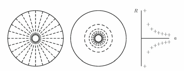
物理代写|理论力学代写theoretical mechanics代考|Curl (Vortex Density)

The curl (rotation) of the vector field $\mathbf{a}(\mathbf{r})$ is the vector field
$$
\operatorname{rot} \mathbf{a} \equiv \nabla \times \mathbf{a} \equiv \lim {V \rightarrow 0} \frac{1}{V} \int{(V)} \mathbf{d} \mathbf{f} \times \mathbf{a}
$$
For the above-mentioned cube with the edges $\mathrm{d} x, \mathrm{~d} y, \mathrm{~d} z$, the $x$-component of the right-hand expression is equal to
$$
\frac{1}{\mathrm{~d} x \mathrm{~d} y \mathrm{~d} z}\left[+\mathrm{d} z \mathrm{~d} x\left{a_{z}(x, y+\mathrm{d} y, z)-a_{z}(x, y, z)\right}\right.
$$
$$
\left.-\mathrm{d} x \mathrm{~d} y\left{a_{y}(x, y, z+\mathrm{d} z)-a_{y}(x, y, z)\right}\right]=\frac{\partial a_{z}}{\partial y}-\frac{\partial a_{y}}{\partial z} .
$$
With $\partial_{i} \equiv 1 / \partial x_{i}$, we thus have
which is the vector product of the operators $\nabla$ and a. This explains the notation $\boldsymbol{\nabla} \times \mathbf{a}$. Moreover, we have
$$
\int_{V} \mathrm{~d} V \nabla \times \mathbf{a}=\int_{(V)} \mathrm{d} \mathbf{f} \times \mathbf{a}
$$
for all continuous vector fields, although they may become singular point-wise, and even along lines, as will become apparent shortly.
An important result is Stokes’s theorem
$$
\int_{A} \mathrm{df} \cdot(\nabla \times \mathbf{a})=\int_{(A)} \mathrm{d} \mathbf{r} \cdot \mathbf{a}
$$
where $\mathrm{df}$ is taken in the rotational sense on the edge $(A)$ and forms a right=hand screw.

物理代写|理论力学代写theoretical mechanics代考|Delta Function

In the following, we shall often use the Dirac delta function. Therefore, its properties are compiled here, even though it does not actually belong to vector analysis, but to general analysis (and in particular to integral calculus).
We start with the Kronecker symbol
$$
\delta_{i k}= \begin{cases}0 & \text { for } i \neq k \ 1 & \text { for } i=k\end{cases}
$$
It is useful for many purposes. In particular we may use it to filter out the $k$ th element of a sequence $\left{f_{i}\right}$ :
$$
f_{k}=\sum_{i} f_{i} \delta_{i k} .
$$
Here, of course, within the sum, one of the $i$ has to take the value $k$. Now, if we make the transition from the countable (discrete) variables $i$ to a continuous quantity $x$, then we must also generalize the Kronecker symbol. This yields Dirac’s delta function $\delta\left(x-x^{\prime}\right)$. It is defined by the equation
$$
f\left(x^{\prime}\right)=\int_{a}^{b} f(x) \delta\left(x-x^{\prime}\right) \mathrm{d} x \quad \text { for } a<x^{\prime}<b, \text { zero otherwise },
$$
where $f(x)$ is an arbitrary continuous test function. If the variable $x$ (and hence also $\mathrm{d} x)$ is a physical quantity with unit $[x]$, the delta function has the unit $[x]^{-1}$.

Obviously, the delta function $\delta\left(x-x^{\prime}\right)$ is not an ordinary function, because it has to vanish for $x \neq x^{\prime}$ and it has to be singular for $x=x^{\prime}$, so that the integral becomes $\int \delta\left(x-x^{\prime}\right) \mathrm{d} x=1$. Consequently, we have to extend the concept of a function: $\delta\left(x-x^{\prime}\right)$ is a distribution, or generalized function, which makes sense only as a weight factor in an integrand, while an ordinary function $y=f(x)$ is a map $x \rightarrow y$. Every equation in which the delta function appears without an integral symbol is an equation between integrands: on both sides of the equation, the integral symbol and the test function have been left out.
The delta function is the derivative of the Heaviside step function:
$$
\varepsilon\left(x-x^{\prime}\right)=\left{\begin{array}{ll}
0 & \text { for } xx^{\prime}
\end{array} \quad \Longrightarrow \quad \delta(x)=\varepsilon^{\prime}(x)\right.
$$

物理代写|理论力学代写theoretical mechanics代考|Fourier Transform

If the region of definition is infinite on both sides, we use
$$
f(x)=\int_{-\infty}^{\infty} g(k, x) f(k) \mathrm{d} k, \quad f(k)=\int_{-\infty}^{\infty} g^{}(k, x) f(x) \mathrm{d} x $$ with $g(k, x)=1 / \sqrt{2 \pi} \exp (\mathrm{i} k x)$ : $$ \begin{aligned} &f(x)=\frac{1}{\sqrt{2 \pi}} \int_{-\infty}^{\infty} \exp (+\mathrm{i} k x) f(k) \mathrm{d} k \ &f(k)=\frac{1}{\sqrt{2 \pi}} \int_{-\infty}^{\infty} \exp (-\mathrm{i} k x) f(x) \mathrm{d} x \end{aligned} $$ Generally, $f(x)$ and $f(k)$ are different functions of their arguments, but we would like to distinguish them only through their argument. [The less symmetric notation $f(x)=\int \exp (\mathrm{i} k x) F(k) \mathrm{d} k$ with $F(k)=f(k) / \sqrt{2 \pi}$ is often used. This avoids the square root factor with the agreement that $(2 \pi)^{-1}$ always appears with $\mathrm{d} x$.] Instead of the pair of variables $x \leftrightarrow k$, the pair $t \leftrightarrow \omega$ is also often used. Important properties of the Fourier transform are $f(x)=f^{}(x) \quad \Longleftrightarrow \quad f(k)=f^{*}(-k)$,
$f(x)=g(x) h(x) \Longleftrightarrow f(k)=\frac{1}{\sqrt{2 \pi}} \int_{-\infty}^{\infty} g\left(k-k^{\prime}\right) h\left(k^{\prime}\right) \mathrm{d} k^{\prime}$,
$f(x)=g\left(x-x^{\prime}\right) \quad \Longleftrightarrow \quad f(k)=\exp \left(-\mathrm{i} k x^{\prime}\right) g(k) .$
For a periodic function $f(x)=f(x-l)$ the last relation leads to the condition $k_{n}=$ $2 \pi n / l$ with $n \in{0, \pm 1, \pm 2, \ldots}$, thus to a Fourier series instead of the integral. In addition, by Fourier transform, all convolution integrals $\int g\left(x-x^{\prime}\right) h\left(x^{\prime}\right) \mathrm{d} x^{\prime}$ can clearly be turned into products $\sqrt{2 \pi} g(k) h(k)$ (Problem 3.9), which are much easier to handle.

理论力学代考

物理代写|理论力学代写theoretical mechanics代考|Curl (Vortex Density)

矢量场的旋度 (旋转) $\mathbf{a}(\mathbf{r})$ 是向量场
$$
\operatorname{rot} \mathbf{a} \equiv \nabla \times \mathbf{a} \equiv \lim V \rightarrow 0 \frac{1}{V} \int(V) \mathbf{d} \mathbf{f} \times \mathbf{a}
$$
对于上述带边的立方体 $\mathrm{d} x, \mathrm{~d} y, \mathrm{~d} z ，$ 这 $x$ – 右手表达式的分量等于
$\backslash$ frac ${1} \backslash \backslash$ mathrm ${\sim \mathrm{d}} \times \backslash m a t h r m{\sim \mathrm{d}}$ y $\backslash$ mathrm ${\sim \mathrm{d}}$ z $} \backslash$ left $\left[+\backslash m a t h r m{\mathrm{~d}} \mathrm{z} \backslash \mathrm{mathrm}{\sim \mathrm{d}} \mathrm{x} \backslash\right.$ left $\left{\mathrm{a}{-}{\mathrm{z}}(\mathrm{x}, \mathrm{y}+\backslash \mathrm{mathrm}{\mathrm{d}}\right.$ y, $\mathrm{z})-\mathrm{a}{-}{$
Veft.-\mathrm{d} x \mathrm{ ${\mathrm{d}} \mathrm{~ y ~ \ l e f t}$
和 $\partial_{i} \equiv 1 / \partial x_{i}$ ，因此我们有
哪个是运算符的向量积 $\nabla$ 和一个。这解释了符号 $\boldsymbol{\nabla} \times \mathbf{a}$. 此外，我们有
$$
\int_{V} \mathrm{~d} V \nabla \times \mathbf{a}=\int_{(V)} \mathrm{d} \mathbf{f} \times \mathbf{a}
$$
对于所有连续向量场，尽管它们可能会逐点变得奇异，甚至沿线变得奇异，这将很快变得显而易见。
一个重要的结果是斯托克斯定理
$$
\int_{A} \mathrm{df} \cdot(\nabla \times \mathbf{a})=\int_{(A)} \mathrm{d} \mathbf{r} \cdot \mathbf{a}
$$
在哪里df是在边缘的旋转方向上拍摄的 $(A)$ 并形成一个右 $=$ 手螺丝。

物理代写|理论力学代写theoretical mechanics代考|Delta Function

下面，我们将经常使用狄拉克函数。因此，这里编译它的性质，尽管它实际上并不属于向量分析，而是属于一般分 析 (尤其是积分)。
我们从克罗内克符号开始
$$
\delta_{i k}={0 \quad \text { for } i \neq k 1 \quad \text { for } i=k
$$
它可用于许多目的。特别是我们可以用它来过滤掉 $k$ 序列的第一个元素[left{f_{i}\right} ：
$$
f_{k}=\sum_{i} f_{i} \delta_{i k} .
$$
这里，当然，在总和中，其中之一i必须取值 $k$. 现在，如果我们从可数 (离散) 变量进行转换 $i$ 到一个连续的量 $x$ ， 那么我们还必须推广克罗内克符号。这产生了狄拉克的 delta 函数 $\delta\left(x-x^{\prime}\right)$. 它由等式定义
$$
f\left(x^{\prime}\right)=\int_{a}^{b} f(x) \delta\left(x-x^{\prime}\right) \mathrm{d} x \quad \text { for } a<x^{\prime}<b, \text { zero otherwise }
$$
在哪里 $f(x)$ 是一个任意的连续测试函数。如果变量 $x$ (因此也 $\mathrm{d} x$ ) 是有单位的物理量 $[x]$, delta 函数有单位 $[x]^{-1}$.
显然，delta函数 $\delta\left(x-x^{\prime}\right)$ 不是一个普通的函数，因为它必须消失 $x \neq x^{\prime}$ 它必须是单数的 $x=x^{\prime}$ ，使得积分变为 $\int \delta\left(x-x^{\prime}\right) \mathrm{d} x=1$. 因此，我们必须扩展函数的概念: $\delta\left(x-x^{\prime}\right)$ 是分布或广义函数，仅作为被积函数中的权 重因子才有意义，而普通函数 $y=f(x)$ 是一张地图 $x \rightarrow y$. delta函数出现而没有积分符号的每一个方程都是被积 函数之间的方程: 在方程的两边，积分符号和测试函数都被省略了。
delta 函数是 Heaviside 阶跃函数的导数：
$\$ \$$
Ivarepsilon $\backslash$ left $(x x \wedge{\backslash$ prime} $\backslash$ right $)=\backslash \operatorname{left}{$
0 for $x x^{\prime}$
Iquad ILongrightarrow \quad Idelta $(x)=$ Ivarepsilon^{1prime $}(x) \backslash$ right.
$\$ \$$

物理代写|理论力学代写theoretical mechanics代考|Fourier Transform

如果定义区域在两边都是无限的，我们使用
$$
f(x)=\int_{-\infty}^{\infty} g(k, x) f(k) \mathrm{d} k, \quad f(k)=\int_{-\infty}^{\infty} g(k, x) f(x) \mathrm{d} x
$$
和 $g(k, x)=1 / \sqrt{2 \pi} \exp (\mathrm{i} k x)$ :
$$
f(x)=\frac{1}{\sqrt{2 \pi}} \int_{-\infty}^{\infty} \exp (+\mathrm{i} k x) f(k) \mathrm{d} k \quad f(k)=\frac{1}{\sqrt{2 \pi}} \int_{-\infty}^{\infty} \exp (-\mathrm{i} k x) f(x) \mathrm{d} x
$$
一般来说， $f(x)$ 和 $f(k)$ 是它们参数的不同功能，但我们只想通过它们的参数来区分它们。[不太对称的符号 $f(x)=\int \exp (\mathrm{i} k x) F(k) \mathrm{d} k$ 和 $F(k)=f(k) / \sqrt{2 \pi}$ 经常使用。这避免了平方根因子与协议 $(2 \pi)^{-1}$ 总是出现 $\mathrm{d} x$ .] 而不是一对变量 $x \leftrightarrow k$ ，这对 $t \leftrightarrow \omega$ 也经常使用。傅里叶变换的重要性质是
$f(x)=f(x) \Longleftrightarrow f(k)=f^{*}(-k)$,
$f(x)=g(x) h(x) \Longleftrightarrow f(k)=\frac{1}{\sqrt{2 \pi}} \int_{-\infty}^{\infty} g\left(k-k^{\prime}\right) h\left(k^{\prime}\right) \mathrm{d} k^{\prime}$
$f(x)=g\left(x-x^{\prime}\right) \Longleftrightarrow f(k)=\exp \left(-\mathrm{i} k x^{\prime}\right) g(k)$
对于周期函数 $f(x)=f(x-l)$ 最后一个关系导致条件 $k_{n}=2 \pi n / l$ 和 $n \in 0, \pm 1, \pm 2, \ldots$ ，因此是傅里叶级数 而不是积分。此外，通过傅里叶变换，所有卷积积分 $\int g\left(x-x^{\prime}\right) h\left(x^{\prime}\right) \mathrm{d} x^{\prime}$ 可以很明显的变成产品
$\sqrt{2 \pi} g(k) h(k)$ (问题 3.9），这更容易处理。

统计代写请认准statistics-lab™. statistics-lab™为您的留学生涯保驾护航。

金融工程代写

金融工程是使用数学技术来解决金融问题。金融工程使用计算机科学、统计学、经济学和应用数学领域的工具和知识来解决当前的金融问题，以及设计新的和创新的金融产品。

非参数统计代写

非参数统计指的是一种统计方法，其中不假设数据来自于由少数参数决定的规定模型；这种模型的例子包括正态分布模型和线性回归模型。

广义线性模型代考

广义线性模型（GLM）归属统计学领域，是一种应用灵活的线性回归模型。该模型允许因变量的偏差分布有除了正态分布之外的其它分布。

术语 广义线性模型（GLM）通常是指给定连续和/或分类预测因素的连续响应变量的常规线性回归模型。它包括多元线性回归，以及方差分析和方差分析（仅含固定效应）。

有限元方法代写

有限元方法（FEM）是一种流行的方法，用于数值解决工程和数学建模中出现的微分方程。典型的问题领域包括结构分析、传热、流体流动、质量运输和电磁势等传统领域。

有限元是一种通用的数值方法，用于解决两个或三个空间变量的偏微分方程（即一些边界值问题）。为了解决一个问题，有限元将一个大系统细分为更小、更简单的部分，称为有限元。这是通过在空间维度上的特定空间离散化来实现的，它是通过构建对象的网格来实现的：用于求解的数值域，它有有限数量的点。边界值问题的有限元方法表述最终导致一个代数方程组。该方法在域上对未知函数进行逼近。[1] 然后将模拟这些有限元的简单方程组合成一个更大的方程系统，以模拟整个问题。然后，有限元通过变化微积分使相关的误差函数最小化来逼近一个解决方案。

tatistics-lab作为专业的留学生服务机构，多年来已为美国、英国、加拿大、澳洲等留学热门地的学生提供专业的学术服务，包括但不限于Essay代写，Assignment代写，Dissertation代写，Report代写，小组作业代写，Proposal代写，Paper代写，Presentation代写，计算机作业代写，论文修改和润色，网课代做，exam代考等等。写作范围涵盖高中，本科，研究生等海外留学全阶段，辐射金融，经济学，会计学，审计学，管理学等全球99%专业科目。写作团队既有专业英语母语作者，也有海外名校硕博留学生，每位写作老师都拥有过硬的语言能力，专业的学科背景和学术写作经验。我们承诺100%原创，100%专业，100%准时，100%满意。

随机分析代写

随机微积分是数学的一个分支，对随机过程进行操作。它允许为随机过程的积分定义一个关于随机过程的一致的积分理论。这个领域是由日本数学家伊藤清在第二次世界大战期间创建并开始的。

时间序列分析代写

随机过程，是依赖于参数的一组随机变量的全体，参数通常是时间。 随机变量是随机现象的数量表现，其时间序列是一组按照时间发生先后顺序进行排列的数据点序列。通常一组时间序列的时间间隔为一恒定值（如1秒，5分钟，12小时，7天，1年），因此时间序列可以作为离散时间数据进行分析处理。研究时间序列数据的意义在于现实中，往往需要研究某个事物其随时间发展变化的规律。这就需要通过研究该事物过去发展的历史记录，以得到其自身发展的规律。

回归分析代写

多元回归分析渐进（Multiple Regression Analysis Asymptotics）属于计量经济学领域，主要是一种数学上的统计分析方法，可以分析复杂情况下各影响因素的数学关系，在自然科学、社会和经济学等多个领域内应用广泛。

MATLAB代写

MATLAB 是一种用于技术计算的高性能语言。它将计算、可视化和编程集成在一个易于使用的环境中，其中问题和解决方案以熟悉的数学符号表示。典型用途包括：数学和计算算法开发建模、仿真和原型制作数据分析、探索和可视化科学和工程图形应用程序开发，包括图形用户界面构建MATLAB 是一个交互式系统，其基本数据元素是一个不需要维度的数组。这使您可以解决许多技术计算问题，尤其是那些具有矩阵和向量公式的问题，而只需用 C 或 Fortran 等标量非交互式语言编写程序所需的时间的一小部分。MATLAB 名称代表矩阵实验室。MATLAB 最初的编写目的是提供对由 LINPACK 和 EISPACK 项目开发的矩阵软件的轻松访问，这两个项目共同代表了矩阵计算软件的最新技术。MATLAB 经过多年的发展，得到了许多用户的投入。在大学环境中，它是数学、工程和科学入门和高级课程的标准教学工具。在工业领域，MATLAB 是高效研究、开发和分析的首选工具。MATLAB 具有一系列称为工具箱的特定于应用程序的解决方案。对于大多数 MATLAB 用户来说非常重要，工具箱允许您学习和应用专业技术。工具箱是 MATLAB 函数（M 文件）的综合集合，可扩展 MATLAB 环境以解决特定类别的问题。可用工具箱的领域包括信号处理、控制系统、神经网络、模糊逻辑、小波、仿真等。

R语言代写	问卷设计与分析代写
PYTHON代写	回归分析与线性模型代写
MATLAB代写	方差分析与试验设计代写
STATA代写	机器学习/统计学习代写
SPSS代写	计量经济学代写
EVIEWS代写	时间序列分析代写
EXCEL代写	深度学习代写
SQL代写	各种数据建模与可视化代写

如果你也在 怎样代写理论力学theoretical mechanics这个学科遇到相关的难题，请随时右上角联系我们的24/7代写客服。

理论力学主要研究物体的力学性能及运动规律，是力学的基础学科，由静力学、运动学和动力学三大部分组成。也有人认为运动学是动力学的一部分，而提出二分法。

statistics-lab™ 为您的留学生涯保驾护航 在代写理论力学theoretical mechanics方面已经树立了自己的口碑, 保证靠谱, 高质且原创的统计Statistics代写服务。我们的专家在代写理论力学theoretical mechanics代写方面经验极为丰富，各种代写理论力学theoretical mechanics相关的作业也就用不着说。

我们提供的理论力学theoretical mechanics及其相关学科的代写，服务范围广, 其中包括但不限于:

• Statistical Inference 统计推断
• Statistical Computing 统计计算
• Advanced Probability Theory 高等概率论
• Advanced Mathematical Statistics 高等数理统计学
• (Generalized) Linear Models 广义线性模型
• Statistical Machine Learning 统计机器学习
• Longitudinal Data Analysis 纵向数据分析
• Foundations of Data Science 数据科学基础

物理代写|理论力学代写theoretical mechanics代考|Vector Fields

If a vector is associated with each position, we speak of a vector field. With scalar fields, a scalar is associated with each position. The vector field $\mathbf{a}(\mathbf{r})$ is only continuous at $\mathbf{r}{0}$ if all paths approaching $\mathbf{r}{0}$ have the same limit. For scalar fields, this is already an essentially stronger requirement than in one dimension.

Instead of drawing a vector field with arrows at many positions, it is often visualized by a set of field lines: at every point of a field line the tangent points in the direction of the vector field. Thus $\mathbf{a} | \mathrm{d} \mathbf{r}$ and $\mathbf{a} \times \mathrm{d} \mathbf{r}=\mathbf{0}$.

For a given vector field many integrals can be formed. In particular, we often have to evaluate integrals over surfaces or volumes. In order to avoid double or triple integral symbols, the corresponding differential is often written immediately after the integral symbol: $\mathrm{d} V$ for the volume, df for the surface integral, e.g., $\int \mathrm{d} \mathbf{f} \times \mathbf{a}$ instead of $-\int \mathbf{a} \times$ df (in this way the unnecessary minus sign is avoided for the introduction of the curl density or rotation on p. 13). Here df is perpendicular to the related surface element. However, the sign of df still has to be fixed. In general, we consider the surface of a volume $V$, which will be denoted here by $(V)$. Then df points outwards. Corresponding to $(V)$, the edge of an area $A$ is denoted by $(A)$.
An important example of a scalar integral is the line integral $\int \mathrm{d} \mathbf{r} \cdot \mathbf{a}(\mathbf{r})$ along a given curve $\mathbf{r}(t)$. If the parameter $t$ determines the points on the curve uniquely, then the line integral $$
\int \mathrm{d} \mathbf{r} \cdot \mathbf{a}(\mathbf{r})=\int \mathrm{d} t \frac{\mathrm{d} \mathbf{r}}{\mathrm{d} t} \cdot \mathbf{a}(\mathbf{r}(t))
$$
is an ordinary integral over the scalar product $\mathbf{a} \cdot \mathrm{d} \mathbf{r} / \mathrm{d} t$. Another example of a scalar integral is the surface integral $\int \mathrm{df} \cdot \mathbf{a}(\mathbf{r})$ taken over a given area $A$ or over the surface $(V)$ of the volume $V$.

Besides the scalar integrals, vectorial integrals like $\int \mathrm{d} V \mathbf{a}, \int \mathrm{d} \mathbf{f} \times \mathbf{a}$, and $\int \mathrm{d} \mathbf{r} \times \mathbf{a}$ can arise, e.g., the $x$-component of $\int \mathrm{d} V$ a is the simple integral $\int \mathrm{d} V a_{x}$.

Different forms are also reasonable through differentiation: vector fields can be deduced from scalar fields, and scalar fields (but also vector fields and tensor fields) from vector fields. These will now be considered one by one. Then the operator $\nabla$ will always turn up. The symbol $\nabla$, an upside-down $\Delta$, resembles an Ancient Greek harp and hence is called nabla, after W. R. Hamilton (see 122).

物理代写|理论力学代写theoretical mechanics代考|Gradient

The gradient of a scalar function $\psi(\mathbf{r})$ is the vector field
$$
\operatorname{grad} \psi \equiv \nabla \psi, \quad \text { with } \nabla \psi \cdot \mathrm{d} \mathbf{r} \equiv \mathrm{d} \psi \equiv \psi(\mathbf{r}+\mathrm{d} \mathbf{r})-\psi(\mathbf{r})
$$
This is clearly perpendicular to the area $\psi=$ const. at every point and points in the direction of $\mathrm{d} \psi>0$ (see Fig. 1.4). The value of the vector $\nabla \psi$ is equal to the derivative of the scalar function $\psi(\mathbf{r})$ with respect to the line element in this direction. In Cartesian coordinates, we thus have
$$
\nabla \psi=\mathbf{e}{x} \frac{\partial \psi}{\partial x}+\mathbf{e}{y} \frac{\partial \psi}{\partial y}+\mathbf{e}{z} \frac{\partial \psi}{\partial z}=\left(\mathbf{e}{x} \frac{\partial}{\partial x}+\mathbf{e}{y} \frac{\partial}{\partial y}+\mathbf{e}{z} \frac{\partial}{\partial z}\right) \psi
$$

Here $\partial \psi / \partial x$ is the partial derivative of $\psi(x, y, z)$ with respect to $x$ for constant $y$ and $z$. (If other quantities are kept fixed instead, then special rules have to be considered, something we shall deal with in Sect. 1.2.7.)
The gradient is also obtained as a limit of a vectorial integral:
$$
\nabla \psi=\lim {V \rightarrow 0} \frac{1}{V} \int{(V)} \text { df } \psi(\mathbf{r})
$$
If we take a cube with infinitesimal edges $\mathrm{d} x, \mathrm{~d} y$, and $\mathrm{d} z$, we have on the right-hand side as $x$-component $(\mathrm{d} x \mathrm{~d} y \mathrm{~d} z)^{-1}{\mathrm{~d} y \mathrm{~d} z \psi(x+\mathrm{d} x, y, z)-\mathrm{d} y \mathrm{~d} z \psi(x, y, z)}=$ $\partial \psi / \partial x$, and similarly for the remaining components. Hence, also
$$
\int_{V} \mathrm{~d} V \nabla \psi-\int_{(V)} \mathrm{d} \mathbf{f} \psi
$$
because a finite volume can be divided into infinitesimal volume elements, and for continuous $\psi$, contributions from adjacent planes cancel in pairs. With this surface integral the gradient can be determined even if $\psi$ is not differentiable (singular) at individual points-the surface integral depends only upon points in the neighbourhood of the singular point, where everything is continuous. (In Sect. 1.1.12, we shall consider the example $\psi=1 / r$.)

物理代写|理论力学代写theoretical mechanics代考|Divergence

While a vector field has been derived from a scalar field with the help of the gradient, the divergence associates a scalar field with a vector field:
$$
\operatorname{div} \mathbf{a} \equiv \nabla \cdot \mathbf{a} \equiv \lim {V \rightarrow 0} \frac{1}{V} \int{(V)} \mathbf{d f} \cdot \mathbf{a}
$$

For the same cube as in the last section, the right-hand expression yields
$$
\begin{aligned}
\frac{1}{\mathrm{~d} x \mathrm{~d} y \mathrm{~d} z} & {\left[\mathrm{~d} y \mathrm{~d} z\left{a_{x}(x+\mathrm{d} x, y, z)-a_{x}(x, y, z)\right}\right.} \
&+\mathrm{d} z \mathrm{~d} x\left{a_{y}(x, y+\mathrm{d} y, z)-a_{y}(x, y, z)\right} \
&\left.+\mathrm{d} x \mathrm{~d} y\left{a_{z}(x, y, z+\mathrm{d} z)-a_{z}(x, y, z)\right}\right]=\frac{\partial a_{x}}{\partial x}+\frac{\partial a_{y}}{\partial y}+\frac{\partial a_{z}}{\partial z}
\end{aligned}
$$
as suggested by the notation $\nabla$. a, i.e., a scalar product between the vector operator $\nabla$ and the vector $\mathbf{a}$. With this we have also proven Gauss’s theorem
$$
\int_{V} \mathrm{~d} V \nabla \cdot \mathbf{a}=\int_{(V)} \mathrm{d} \mathbf{f} \cdot \mathbf{a}
$$
since for any partition of the finite volume $V$ into infinitesimal ones and for a continuous vector field $\mathbf{a}$, the contributions of adjacent planes cancel in pairs. The integrals here may even enclose points at which a (r) is singular (see Fig. 1.5 left). We shall discuss this in more detail in Sect. 1.1.12.

The integral $\int$ df $\cdot \mathbf{a}$ over an area is called the $\int u x$ of the vector field $\mathbf{a}(\mathbf{r})$ through this area (even if $\mathbf{a}$ is not a current density). In this picture, the integral over the closed area $(V)$ describes the source strength of the vector field, i.e., how much more flows into $V$ than out. The divergence is therefore to be understood as a source density. A vector field is said to be source-free if its divergence vanishes everywhere. (If the source density is negative, then “drains” predominate.)

The concept of a field-line tube is also useful (we discussed field lines in Sect. 1.1.4). Its walls are everywhere parallel to a (r). Therefore, there is no flux through the walls, and the flux through the end faces is equal to the volume integral of $\nabla \cdot \mathbf{a}$. For a source-free vector field $(\nabla \cdot \mathbf{a}=0)$, the flux flowing into the field-line tube through one end face emerges again from the other.

理论力学代考

物理代写|理论力学代写theoretical mechanics代考|Vector Fields

如果一个向量与每个位置相关联，我们就说一个向量场。对于标量字段，标量与每个位置相关联。向量场 $\mathbf{a}(\mathbf{r})$ 仅 在 $\mathbf{r} 0$ 如果所有路径都接近 $r 0$ 有相同的限制。对于标量场，这已经是比一维更严格的要求。
它不是在许多位置绘制带有箭头的矢量场，而是通常通过一组场线来可视化: 在场线的每个点处，切点在矢量场的 方向上。因此 $\mathbf{a} \mid \mathrm{d} \mathbf{r}$ 和 $\mathbf{a} \times \mathrm{d} \mathbf{r}=\mathbf{0}$.
对于给定的向量场，可以形成许多积分。特别是，我们经常需要评估曲面或体积上的积分。为了避免双重或三重积 分符号，对应的溦分通常写在积分符号之后： $\mathrm{d} V$ 为体积， $\mathrm{df}$ 为表面积分，例如， $\int \mathrm{d} \mathbf{f} \times \mathbf{a}$ 代替 $-\int \mathbf{a} \times \mathrm{df}$ (通过 这种方式，避免了在第 13 页引入卷曲密度或旋转时不必要的减号)。这里 df 垂直于相关的表面元素。但是， $d f$ 的符号仍需修正。通常，我们考虑体积的表面 $V$ ，这里用 $(V)$. 然后 df 指向外面。对应 $(V)$ ，一个区域的边缘 $A$ 表示 为 $(A)$.
标量积分的一个重要例子是线积分 $\int \mathrm{d} \mathbf{r} \cdot \mathbf{a}(\mathbf{r})$ 沿着给定的曲线 $\mathbf{r}(t)$. 如果参数唯一确定曲线上的点，然后线积分
$$
\int \mathrm{d} \mathbf{r} \cdot \mathbf{a}(\mathbf{r})=\int \mathrm{d} t \frac{\mathrm{d} \mathbf{r}}{\mathrm{d} t} \cdot \mathbf{a}(\mathbf{r}(t))
$$
是标量积上的普通积分 $\mathbf{a} \cdot \mathrm{d} \mathbf{r} / \mathrm{d} t$. 标量积分的另一个例子是表面积分 $\int \mathrm{df} \cdot \mathbf{a}(\mathbf{r})$ 接管给定区域 $A$ 或表面上 $(V)$ 体 积的 $V$.
除了标量积分，向量积分如 $\int \mathrm{d} V \mathbf{a}, \int \mathrm{d} \mathbf{f} \times \mathbf{a}$ ，和 $\int \mathrm{d} \mathbf{r} \times \mathbf{a}$ 可能会出现，例如， $x$ – 的组成部分 $\int \mathrm{d} V \mathrm{a}$ 是简单积 分 $\int \mathrm{d} V a_{x}$
不同的形式通过微分也是合理的: 向量场可以从标量场推导出来，标量场（也可以是向量场和张量场) 从向量场推 导出来。这些现在将被一一考虑。那么运营商 $\nabla$ 总会出现的。符号 $\nabla$ ，一个颠倒的 $\Delta$ ，类似于古希腊竖琴，因此在 WR Hamilton 之后被称为 nabla（见 122）。

物理代写|理论力学代写theoretical mechanics代考|Gradient

标量函数的梯度 $\psi(\mathbf{r})$ 是向量场
$$
\operatorname{grad} \psi \equiv \nabla \psi, \quad \text { with } \nabla \psi \cdot \mathrm{d} \mathbf{r} \equiv \mathrm{d} \psi \equiv \psi(\mathbf{r}+\mathrm{d} \mathbf{r})-\psi(\mathbf{r})
$$
这显然垂直于该区域 $\psi=$ 常量。在每个点和指向的方向 $\mathrm{d} \psi>0$ (见图 1.4) 。向量的值 $\nabla \psi$ 等于标量函数的导数 $\psi(\mathbf{r})$ 相对于这个方向的线元素。在笛卡尔坐标中，我们因此有
$$
\nabla \psi=\mathbf{e} x \frac{\partial \psi}{\partial x}+\mathbf{e} y \frac{\partial \psi}{\partial y}+\mathbf{e} z \frac{\partial \psi}{\partial z}=\left(\mathbf{e} x \frac{\partial}{\partial x}+\mathbf{e} y \frac{\partial}{\partial y}+\mathbf{e} z \frac{\partial}{\partial z}\right) \psi
$$
这里 $\partial \psi / \partial x$ 是的偏导数 $\psi(x, y, z)$ 关于 $x$ 为常数 $y$ 和 $z$. (如果其他量保持不变，则必须考虑特殊规则，我们将在第 $1.2 .7$ 节中讨论。)
梯度也作为矢量积分的极限获得:
$$
\nabla \psi=\lim V \rightarrow 0 \frac{1}{V} \int(V) \mathrm{df} \psi(\mathbf{r})
$$
如果我们取一个具有无穷小边的立方体 $\mathrm{d} x, \mathrm{~d} y$ ，和 $\mathrm{d} z$ ，我们在右边有 $x$-零件
$(\mathrm{d} x \mathrm{~d} y \mathrm{~d} z)^{-1} \mathrm{~d} y \mathrm{~d} z \psi(x+\mathrm{d} x, y, z)-\mathrm{d} y \mathrm{~d} z \psi(x, y, z)=\partial \psi / \partial x$ ，对于其余的组件也是如此。因此，也
$$
\int_{V} \mathrm{~d} V \nabla \psi-\int_{(V)} \mathrm{d} \mathbf{f} \psi
$$
因为一个有限的体积可以分成无穷小的体积元素，而对于连续的 $\psi$ ，来自相邻平面的贡献成对抵消。使用这个表面 积分，即使在以下情况下也可以确定梯度 $\psi$ 在单个点上是不可微的（奇异的) – 曲面积分仅取决于奇异点附近的 点，其中一切都是连续的。（在第 $1.1 .12$ 节中，我们将考虑这个例子 $\psi=1 / r$.)

物理代写|理论力学代写theoretical mechanics代考|Divergence

虽然向量场是在梯度的帮助下从标量场导出的，但散度将标量场与向量场相关联:
$\$ \$$
loperatorname{div} \mathbf{a} \equiv $\backslash$ nabla $\backslash$ cdot $\backslash$ mathbf ${$ a $}$ lequiv $\backslash \lim {V \backslash$ Irightarrow 0$} \backslash$ frac ${1} V} \backslash$ Iint ${(\mathrm{V})} \mathrm{~ I m a t h b f { d f } ~ \ c d o t ~ \ m a t h b f { a }}$
$\$ \$$
对于与上一节中相同的立方体，右侧表达式产生
Ibegin ${a l i g n} \backslash$ frac ${1} \backslash \backslash m a t h r m{\sim d} x \backslash m a t h r m{\sim d}$ 和 $\backslash$ mathrm ${\sim d}$ Z \& ${\backslash \backslash$ eft $\backslash \backslash m a t h r m{\sim d}$ 和 $\backslash$ mathrm ${\sim d}}$ Z $\backslash$ eft ${a$
正如符号所建议的那样 $\nabla$. a，即向量算子之间的标量积 $\nabla$ 和向量 $\mathbf{a}$. 这样我们也证明了高斯定理
$$
\int_{V} \mathrm{~d} V \nabla \cdot \mathbf{a}=\int_{(V)} \mathrm{d} \mathbf{f} \cdot \mathbf{a}
$$
因为对于有限体积的任何分区 $V$ 成无穷小和连续向量场 $\mathbf{a}$ ，相邻平面的贡献成对抵消。这里的积分甚至可以包含 $a$ (r) 为奇异的点 (见图 $1.5$ 左) 。我们将在第 3 节中更详细地讨论这个问题。1.1.12。
积分 $\int \mathrm{df} \cdot \mathbf{a}$ 在一个区域上称为 $\int u x$ 向量场的 $\mathbf{a}(\mathbf{r})$ 通过这个区域（即使 $\mathbf{a}$ 不是电流密度）。在这张图中，封闭区域上 的积分 $(V)$ 描述矢量场的源强度，即有多少流入 $V$ 比出来。因此，该分歧应被理解为源密度。如果矢量场的散度处 处消失，则称矢量场是无源的。（如果源密度为负，则漏极”占主导地位。）
场线管的概念也很有用（我们在第 $1.1 .4$ 节中讨论了场线）。它的墙壁处处平行于 $a(r)$ 。因此，没有通过壁的通 量，通过端面的通量等于体积积分 $\nabla \cdot \mathbf{a}$. 对于无源矢量场 $(\nabla \cdot \mathbf{a}=0)$ ，通过一个端面流入场线管的通量从另一个 端面再次出现。

统计代写请认准statistics-lab™. statistics-lab™为您的留学生涯保驾护航。

金融工程代写

金融工程是使用数学技术来解决金融问题。金融工程使用计算机科学、统计学、经济学和应用数学领域的工具和知识来解决当前的金融问题，以及设计新的和创新的金融产品。

非参数统计代写

非参数统计指的是一种统计方法，其中不假设数据来自于由少数参数决定的规定模型；这种模型的例子包括正态分布模型和线性回归模型。

广义线性模型代考

广义线性模型（GLM）归属统计学领域，是一种应用灵活的线性回归模型。该模型允许因变量的偏差分布有除了正态分布之外的其它分布。

术语 广义线性模型（GLM）通常是指给定连续和/或分类预测因素的连续响应变量的常规线性回归模型。它包括多元线性回归，以及方差分析和方差分析（仅含固定效应）。

有限元方法代写

有限元方法（FEM）是一种流行的方法，用于数值解决工程和数学建模中出现的微分方程。典型的问题领域包括结构分析、传热、流体流动、质量运输和电磁势等传统领域。

有限元是一种通用的数值方法，用于解决两个或三个空间变量的偏微分方程（即一些边界值问题）。为了解决一个问题，有限元将一个大系统细分为更小、更简单的部分，称为有限元。这是通过在空间维度上的特定空间离散化来实现的，它是通过构建对象的网格来实现的：用于求解的数值域，它有有限数量的点。边界值问题的有限元方法表述最终导致一个代数方程组。该方法在域上对未知函数进行逼近。[1] 然后将模拟这些有限元的简单方程组合成一个更大的方程系统，以模拟整个问题。然后，有限元通过变化微积分使相关的误差函数最小化来逼近一个解决方案。

tatistics-lab作为专业的留学生服务机构，多年来已为美国、英国、加拿大、澳洲等留学热门地的学生提供专业的学术服务，包括但不限于Essay代写，Assignment代写，Dissertation代写，Report代写，小组作业代写，Proposal代写，Paper代写，Presentation代写，计算机作业代写，论文修改和润色，网课代做，exam代考等等。写作范围涵盖高中，本科，研究生等海外留学全阶段，辐射金融，经济学，会计学，审计学，管理学等全球99%专业科目。写作团队既有专业英语母语作者，也有海外名校硕博留学生，每位写作老师都拥有过硬的语言能力，专业的学科背景和学术写作经验。我们承诺100%原创，100%专业，100%准时，100%满意。

随机分析代写

随机微积分是数学的一个分支，对随机过程进行操作。它允许为随机过程的积分定义一个关于随机过程的一致的积分理论。这个领域是由日本数学家伊藤清在第二次世界大战期间创建并开始的。

时间序列分析代写

随机过程，是依赖于参数的一组随机变量的全体，参数通常是时间。 随机变量是随机现象的数量表现，其时间序列是一组按照时间发生先后顺序进行排列的数据点序列。通常一组时间序列的时间间隔为一恒定值（如1秒，5分钟，12小时，7天，1年），因此时间序列可以作为离散时间数据进行分析处理。研究时间序列数据的意义在于现实中，往往需要研究某个事物其随时间发展变化的规律。这就需要通过研究该事物过去发展的历史记录，以得到其自身发展的规律。

回归分析代写

多元回归分析渐进（Multiple Regression Analysis Asymptotics）属于计量经济学领域，主要是一种数学上的统计分析方法，可以分析复杂情况下各影响因素的数学关系，在自然科学、社会和经济学等多个领域内应用广泛。

MATLAB代写

MATLAB 是一种用于技术计算的高性能语言。它将计算、可视化和编程集成在一个易于使用的环境中，其中问题和解决方案以熟悉的数学符号表示。典型用途包括：数学和计算算法开发建模、仿真和原型制作数据分析、探索和可视化科学和工程图形应用程序开发，包括图形用户界面构建MATLAB 是一个交互式系统，其基本数据元素是一个不需要维度的数组。这使您可以解决许多技术计算问题，尤其是那些具有矩阵和向量公式的问题，而只需用 C 或 Fortran 等标量非交互式语言编写程序所需的时间的一小部分。MATLAB 名称代表矩阵实验室。MATLAB 最初的编写目的是提供对由 LINPACK 和 EISPACK 项目开发的矩阵软件的轻松访问，这两个项目共同代表了矩阵计算软件的最新技术。MATLAB 经过多年的发展，得到了许多用户的投入。在大学环境中，它是数学、工程和科学入门和高级课程的标准教学工具。在工业领域，MATLAB 是高效研究、开发和分析的首选工具。MATLAB 具有一系列称为工具箱的特定于应用程序的解决方案。对于大多数 MATLAB 用户来说非常重要，工具箱允许您学习和应用专业技术。工具箱是 MATLAB 函数（M 文件）的综合集合，可扩展 MATLAB 环境以解决特定类别的问题。可用工具箱的领域包括信号处理、控制系统、神经网络、模糊逻辑、小波、仿真等。

R语言代写	问卷设计与分析代写
PYTHON代写	回归分析与线性模型代写
MATLAB代写	方差分析与试验设计代写
STATA代写	机器学习/统计学习代写
SPSS代写	计量经济学代写
EVIEWS代写	时间序列分析代写
EXCEL代写	深度学习代写
SQL代写	各种数据建模与可视化代写

如果你也在 怎样代写理论力学theoretical mechanics这个学科遇到相关的难题，请随时右上角联系我们的24/7代写客服。

理论力学主要研究物体的力学性能及运动规律，是力学的基础学科，由静力学、运动学和动力学三大部分组成。也有人认为运动学是动力学的一部分，而提出二分法。

statistics-lab™ 为您的留学生涯保驾护航 在代写理论力学theoretical mechanics方面已经树立了自己的口碑, 保证靠谱, 高质且原创的统计Statistics代写服务。我们的专家在代写理论力学theoretical mechanics代写方面经验极为丰富，各种代写理论力学theoretical mechanics相关的作业也就用不着说。

我们提供的理论力学theoretical mechanics及其相关学科的代写，服务范围广, 其中包括但不限于:

• Statistical Inference 统计推断
• Statistical Computing 统计计算
• Advanced Probability Theory 高等概率论
• Advanced Mathematical Statistics 高等数理统计学
• (Generalized) Linear Models 广义线性模型
• Statistical Machine Learning 统计机器学习
• Longitudinal Data Analysis 纵向数据分析
• Foundations of Data Science 数据科学基础

物理代写|理论力学代写theoretical mechanics代考|Space and Time

Space and time are two basic concepts which, according to Kant, inherently or innately determine the form of all experience in an a priori manner, thereby making possible experience as such: only in space and time can we arrange our sensations. [According to the doctrines of evolutionary cognition, what is innate to us has developed phylogenetically by adaption to our environment. This is why we only notice the insufficiency of these “self-evident”‘ concepts under extraordinary circumstances, e.g., for velocities close to that of light $\left(c_{0}\right)$ or actions of the order of Planck’s quantum $h$. We shall tackle such “weird” cases later-in electromagnetism and quantum mechanics. For the time being, we want to make sure we can handle our familiar environment.]

To do this, we introduce a continuous parameter $t$. Like every other physical quantity it is composed of number and unit (for example, a second $1 \mathrm{~s}=1 \mathrm{~min} / 60$ $-1 \mathrm{~h} / 3600$ ). The larger the unit, the smaller the number. Physical quantities do not depend on the unit-likewise equations between physical quantities. Nevertheless, the opposite is sometimes seen, as in: “We choose units such that the velocity of light $c$ assumes the value 1”. In fact, the concept of velocity is thereby changed, so that instead of the velocity $v$, the ratio $v / c$ is taken here as the velocity, and $c t$ as time or $x / c$ as length.

The zero time $(t=0)$ can be chosen arbitrarily, since basically only the time difference, i.e., the duration of a process, is important. A differentiation with respect to time $(\mathrm{d} / \mathrm{d} t)$ is often marked by a dot over the differentiated quantity, i.e., $\mathrm{d} x / \mathrm{d} t \equiv \dot{x}$.
In empty space every direction is equivalent. Here, too, we may choose the zero point freely and, starting from this point, determine the position of other points in a coordinate-free notation by the position vector $\mathbf{r}$, which fixes the distance and direction of the point under consideration. This coordinate-free type of notation is particularly advantageous when we want to exploit the assumed homogeneity of space. However, conditions often arise (i.e., when there is axial or spherical symmetry) which are best taken care of in special coordinates. We are free to choose a coordinate system. We only require that it determine all positions uniquely. This we shall treat in the next section.

物理代写|理论力学代写theoretical mechanics代考|Vector Algebra

From two vectors $\mathbf{a}$ and $\mathbf{b}$, their sum $\mathbf{a}+\mathbf{b}$ may be formed according to the construction of parallelograms (as the diagonal), as shown in Fig. 1.1. From this follows the commutative and associative law of vector addition:
$$
\mathbf{a}+\mathbf{b}=\mathbf{b}+\mathbf{a}, \quad(\mathbf{a}+\mathbf{b})+\mathbf{c}=\mathbf{a}+(\mathbf{b}+\mathbf{c})
$$
The product of the vectors a with a scalar (i.e., directionless) factor $\alpha$ is understood as the vector $\alpha \mathbf{a}=\mathbf{a} \alpha$ with the same (for $\alpha<0$ opposite) direction and with value $|\alpha| a$. In particular, a and $-\mathbf{a}$ have the same value, but opposite directions. For $\alpha=0$ the zero vector 0 results, with length 0 and undetermined direction.

The scalar product (inner product) $\mathbf{a} \cdot \mathbf{b}$ of the two vectors $\mathbf{a}$ and $\mathbf{b}$ is the product of their values times the cosine of the enclosed angle $\phi_{a b}$ (see Fig. 1.2 left):
$$
\mathbf{a} \cdot \mathbf{b} \equiv a b \cos \phi_{a b}
$$
The dot between the two factors is important for the scalar product-if it is missing, then it is the tensor product of the two vectors, which will be explained in Sect. 1.2.4 with $\mathbf{a} \cdot \mathbf{b} \mathbf{c} \neq \mathbf{a} \mathbf{b} \cdot \mathbf{c}$, if $\mathbf{a}$ and $\mathbf{c}$ have different directions, i.e., if $\mathbf{a}$ is not a multiple of $\mathbf{c}$. Consequently, one has
$$
\mathbf{a} \cdot \mathbf{b}=\mathbf{b} \cdot \mathbf{a}
$$
and
$$
\mathbf{a} \cdot \mathbf{b}=0 \quad \Longleftrightarrow \quad \mathbf{a} \perp \mathbf{b} \text { or } a=0 \text { or } b=0 .
$$
If the two vectors are oriented perpendicularly to each other $(\mathbf{a} \perp \mathbf{b})$, then they are also said to be orthogonal. Obviously, $\mathbf{a} \cdot \mathbf{a}=a^{2}$ holds. Vectors with value 1 are called unit vectors. Here they are denoted by e. Given three Cartesian, i.e., pairwise perpendicular unit vectors $\mathbf{e}{x}, \mathbf{e}{y}, \mathbf{e}{z}$, all vectors can be decomposed in terms of these: $$ \mathbf{a}=\mathbf{e}{x} a_{x}+\mathbf{e}{y} a{y}+\mathbf{e}{z} a{z},
$$
with the Cartesian components
$$
a_{x} \equiv \mathbf{e}{x} \cdot \mathbf{a}, \quad a{y} \equiv \mathbf{e}{y} \cdot \mathbf{a}, \quad a{z} \equiv \mathbf{e}_{z} \cdot \mathbf{a} .
$$

物理代写|理论力学代写theoretical mechanics代考|Trajectories

If a vector depends upon a parameter, then we speak of a vector function. The vector function $\mathbf{a}(t)$ is continuous at $t_{0}$, if it tends to $\mathbf{a}\left(t_{0}\right)$ for $t \rightarrow t_{0}$. With the same limit $t \rightarrow t_{0}$, the vector differential da and the first derivative da/d $t$ is introduced. These quantities may be formed for every Cartesian component, and we have
$$
\begin{array}{ll}
\mathrm{d}(\mathbf{a}+\mathbf{b})=\mathrm{d} \mathbf{a}+\mathrm{d} \mathbf{b}, & \mathrm{d}(\alpha \mathbf{a})=\alpha \mathrm{d} \mathbf{a}+\mathbf{a} \mathrm{d} \alpha \
\mathrm{d}(\mathbf{a} \cdot \mathbf{b})=\mathbf{a} \cdot \mathrm{d} \mathbf{b}+\mathbf{b} \cdot \mathrm{d} \mathbf{a}, & \mathrm{d}(\mathbf{a} \times \mathbf{b})=\mathbf{a} \times \mathrm{d} \mathbf{b}-\mathbf{b} \times \mathrm{d} \mathbf{a}
\end{array}
$$
Obviously, $\mathbf{a} \cdot \mathrm{d} \mathbf{a} / \mathrm{d} t=\frac{1}{2} \mathrm{~d}(\mathbf{a} \cdot \mathbf{a}) / \mathrm{d} t=\frac{1}{2} \mathrm{~d} a^{2} / \mathrm{d} t=a \mathrm{~d} a / \mathrm{d} t$ holds. In particular the derivative of a unit vector is always perpendicular to the original vector-if it does nôt vañish.

As an example of a vector function, we investigate $\mathbf{r}(t)$, the path of a point as a function of the time $t$. Thus we want to consider also the velocity $\mathbf{v}=\dot{\mathbf{r}}$ and the acceleration $\mathbf{a}=\ddot{\mathbf{r}}$ rather generally. The time is not important for the trajectories as geometrical lines. Therefore, instead of the time $t$ we introduce the path length $s$ as a parameter and exploit $\mathrm{d} s=|\mathrm{d} \mathbf{r}|=v \mathrm{~d} t$.

We now take three mutually perpendicular unit vectors $\mathbf{e}{\mathrm{T}}, \mathbf{e}{\mathrm{N}}$, and $\mathbf{e}{\mathrm{B}}$, which are attached to every point on the trajectory. Here $\mathbf{e}{\mathrm{T}}$ has the direction of $\mathbf{v}$ :
tangent vector $\quad \mathbf{e}{\mathrm{T}} \equiv \frac{\mathrm{d} \mathbf{r}}{\mathrm{d} s}=\frac{\mathbf{v}}{v}$ For a straight path, this vector is already sufficient for the description. But in general the path curvature $\quad \kappa \equiv\left|\frac{\mathrm{d} \mathbf{e}{\mathrm{T}}}{\mathrm{d} s}\right|=\left|\frac{\mathrm{d}^{2} \mathbf{r}}{\mathrm{d} s^{2}}\right|$
is different from zero. In order to get more insight into this parameter we consider a plane curve of constant curvature, namely, the circle with $s=R \varphi$. For $\mathbf{r}(\varphi)=\mathbf{r}{0}+$ $R\left(\cos \varphi \mathbf{e}{x}+\sin \varphi \mathbf{e}{y}\right)$, we have $\kappa=\left|\mathrm{d}^{2} \mathbf{r} / \mathrm{d}(R \varphi)^{2}\right|=R^{-1}$. Instead of the curvature $\kappa$, its reciprocal, the curvature radius $R \equiv \frac{1}{\kappa}$, can also be used to determine the curve. Hence as a further unit vector we have the normal vector $\quad \mathbf{e}{\mathrm{N}} \equiv R \frac{\mathbf{d} \mathbf{e}_{\mathrm{T}}}{\mathrm{d} s}=R \frac{\mathrm{d}^{2} \mathbf{r}}{\mathrm{d} s^{2}}$

理论力学代考

物理代写|理论力学代写theoretical mechanics代考|Space and Time

空间和时间是两个基本概念，在康德看来，它们先天地或先天地决定了所有经验的形式，从而使经验本身成为可 能: 只有在空间和时间中，我们才能安排我们的感觉。[根据进化认知的学说，我们与生倶来的东西是通过适应我 们的环境而在系统发育上发展起来的。这就是为什么我们只注意到这些”不言而喻”的概念在特殊情况下的不足之 处，例如，对于接近光速的速度 $\left(c_{0}\right)$ 或普朗克量子级的动作 $h$. 我们将在稍后的电磁学和量子力学中解决这些”奇怪” 的情况。目前，我们希望确保我们能够处理我们熟悉的环境。]
为此，我们引入了一个连续参数 $t$. 像所有其他物理量一样，它由数字和单位组成（例如，一秒 $1 \mathrm{~s}=1 \mathrm{~min} / 60$ $-1 \mathrm{~h} / 3600$ ) 。单位越大，数字越小。物理量不依赖于物理量之间的类似单位方程。然而，有时会看到相反的情 况，例如: “我们选择单位使得光速 $c$ 假定值为 1 “。事实上，速度的概念因此而改变，因此速度代替了速度 $v$ ，比例 $v / c$ 这里取为速度，并且 $c t$ 作为时间或 $x / c$ 作为长度。
零时 $(t=0)$ 可以任意选择，因为基本上只有时间差，即一个过程的持续时间，是重要的。时间上的差异化 $(\mathrm{d} / \mathrm{d} t)$ 通常在微分数量上用一个点标记，即 $\mathrm{d} x / \mathrm{d} t \equiv \dot{x}$.
在空旷的空间中，每个方向都是等价的。在这里，我们也可以自由选择零点，并从该点开始，通过位置向量以无坐 标表示法确定其他点的位置r，它固定了所考虑点的距离和方向。当我们想要利用假设的空间同质性时，这种无坐 标类型的符号特别有利。然而，通常会出现一些情况（即，当存在轴对称或球对称时），最好在特殊坐标中处理这 些情况。我们可以自由选择坐标系。我们只要求它唯一地确定所有位置。这一点我们将在下一节中讨论。

物理代写|理论力学代写theoretical mechanics代考|Vector Algebra

从两个向量 $\mathbf{a}$ 和 $\mathbf{b}$, 他们的总和 $\mathbf{a}+\mathbf{b}$ 可以根据平行四边形的构造 (作为对角线) 形成，如图 $1.1$ 所示。由此遵㑑向 量加法的交换结合律：
$$
\mathbf{a}+\mathbf{b}=\mathbf{b}+\mathbf{a}, \quad(\mathbf{a}+\mathbf{b})+\mathbf{c}=\mathbf{a}+(\mathbf{b}+\mathbf{c})
$$
向量 $\mathrm{a}$ 与标量 (即无方向) 因子的乘积 $\alpha$ 被理解为向量 $\alpha \mathbf{a}=\mathbf{a} \alpha$ 同样 (对于 $\alpha<0$ 相反) 方向和价值 $|\alpha| a$. 特别 是，一个和 $-\mathbf{a}$ 具有相同的值，但方向相反。为了 $\alpha=0$ 零向量 0 结果，长度为 0 ，方向末定。
标量积 (内积) $\mathbf{a} \cdot \mathbf{b}$ 两个向量的和b是它们的值乘以封闭角的余弦的乘积 $\phi_{a b}$ (见图 $1.2$ 左）：
$$
\mathbf{a} \cdot \mathbf{b} \equiv a b \cos \phi_{a b}
$$
两个因子之间的点对于标量积很重要一一如果它缺失了，那么它就是两个向量的张量积，这将在 Sect. 1.2.4与 $\mathbf{a} \cdot \mathbf{b c} \neq \mathbf{a b} \cdot \mathbf{c}$ ，如果 $\mathbf{a}$ 和 $\mathbf{c}$ 有不同的方向，即，如果 $\mathbf{a}$ 不是的倍数 $\mathbf{c}$. 因此，一个有
$$
\mathbf{a} \cdot \mathbf{b}=\mathbf{b} \cdot \mathbf{a}
$$
和
$$
\mathbf{a} \cdot \mathbf{b}=0 \quad \Longleftrightarrow \quad \mathbf{a} \perp \mathbf{b} \text { or } a=0 \text { or } b=0
$$
如果两个向量相互垂直 $(\mathbf{a} \perp \mathbf{b})$ ，那么它们也被称为正交的。明显地， $\mathbf{a} \cdot \mathbf{a}=a^{2}$ 持有。值为 1 的向量称为单位 向量。在这里，它们用 e 表示。给定三个笛卡尔，即成对的垂直单位向量 $\mathbf{e} x, \mathbf{e} y, \mathbf{e} z$ ，所有向量都可以按照以下方 式分解:
$$
\mathbf{a}=\mathbf{e} x a_{x}+\mathbf{e} y a y+\mathbf{e} z a z
$$
使用笛卡尔分量
$$
a_{x} \equiv \mathbf{e} x \cdot \mathbf{a}, \quad a y \equiv \mathbf{e} y \cdot \mathbf{a}, \quad a z \equiv \mathbf{e}_{z} \cdot \mathbf{a} .
$$

物理代写|理论力学代写theoretical mechanics代考|Trajectories

如果一个向量依赖于一个参数，那么我们就说一个向量函数。向量函数 $\mathbf{a}(t)$ 是连续的 $t_{0}$ ，如果它倾向于 $\mathbf{a}\left(t_{0}\right)$ 为了 $t \rightarrow t_{0}$. 具有相同的限制 $t \rightarrow t_{0}$ ，向量微分 $\mathrm{da}$ 和一阶导数 $\mathrm{da} / \mathrm{d} t$ 介绍。这些量可以为每个笛卡尔分量形成，我们] 有
$$
\mathrm{d}(\mathbf{a}+\mathbf{b})=\mathrm{d} \mathbf{a}+\mathrm{d} \mathbf{b}, \quad \mathrm{d}(\alpha \mathbf{a})=\alpha \mathrm{d} \mathbf{a}+\mathbf{a d} \alpha \mathrm{d}(\mathbf{a} \cdot \mathbf{b})=\mathbf{a} \cdot \mathrm{d} \mathbf{b}+\mathbf{b} \cdot \mathrm{d} \mathbf{a}, \quad \mathrm{d}(\mathbf{a} \times \mathbf{b})=\mathbf{a} \times \mathrm{d} \mathbf{b}-\mathbf{b} \times \mathrm{d}
$$
明显地， $\mathbf{a} \cdot \mathrm{d} \mathbf{a} / \mathrm{d} t=\frac{1}{2} \mathrm{~d}(\mathbf{a} \cdot \mathbf{a}) / \mathrm{d} t=\frac{1}{2} \mathrm{~d} a^{2} / \mathrm{d} t=a \mathrm{~d} a / \mathrm{d} t$ 持有。特别是单位向量的导数总是垂直于原始 向量一一如果它不消失的话。
作为向量函数的一个例子，我们研究 $\mathbf{r}(t)$, 作为时间函数的点的路径t. 因此，我们还想考虑速度 $\mathbf{v}=\dot{\mathbf{r}}$ 和加速度 $\mathbf{a}=\ddot{\mathbf{r}}$ 相当普遍。对于作为几何线的轨迹来说，时间并不重要。因此，而不是时间 $t$ 我们引入路径长度 $s$ 作为参数并 利用 $\mathrm{d} s=|\mathrm{d} \mathbf{r}|=v \mathrm{~d} t$.
我们现在取三个相互垂直的单位向量eT $\mathrm{eN}$ ，和 $e B$ ，它们附加到轨迹上的每个点。这里eT有方向 $v:$ 切向量 $\quad \mathbf{e T} \equiv \frac{\mathrm{dr}}{\mathrm{d} s}=\frac{\mathrm{v}}{v}$ 对于直线路径，这个向量已经足够描述了。但总的来说路径曲率 $\quad \kappa \equiv\left|\frac{\mathrm{deT}}{\mathrm{d} s}\right|=\left|\frac{\mathrm{d}^{2} \mathrm{r}}{\mathrm{d} s^{2}}\right|$ 不同于零。为了更深入地了解这个参数，我们考虑一个恒定曲率的平面曲线，即圆 $s=R \varphi$. 为了 $\mathbf{r}(\varphi)=\mathbf{r} 0+$ $R(\cos \varphi \mathbf{e} x+\sin \varphi \mathbf{e} y)$ ，我们有 $\kappa=\left|\mathrm{d}^{2} \mathbf{r} / \mathrm{d}(R \varphi)^{2}\right|=R^{-1}$. 而不是曲率 $\kappa$ ，它的倒数，曲率半径 $R \equiv \frac{1}{\kappa}$ ，也 可用于确定曲线。因此，作为进一步的单位向量，我们有法线向量 $\mathrm{eN} \equiv R \frac{\mathrm{de} \mathrm{T}}{\mathrm{d} s}=R \frac{\mathrm{d}^{2} \mathrm{r}}{\mathrm{d} s^{2}}$

统计代写请认准statistics-lab™. statistics-lab™为您的留学生涯保驾护航。

金融工程代写

金融工程是使用数学技术来解决金融问题。金融工程使用计算机科学、统计学、经济学和应用数学领域的工具和知识来解决当前的金融问题，以及设计新的和创新的金融产品。

非参数统计代写

非参数统计指的是一种统计方法，其中不假设数据来自于由少数参数决定的规定模型；这种模型的例子包括正态分布模型和线性回归模型。

广义线性模型代考

广义线性模型（GLM）归属统计学领域，是一种应用灵活的线性回归模型。该模型允许因变量的偏差分布有除了正态分布之外的其它分布。

术语 广义线性模型（GLM）通常是指给定连续和/或分类预测因素的连续响应变量的常规线性回归模型。它包括多元线性回归，以及方差分析和方差分析（仅含固定效应）。

有限元方法代写

有限元方法（FEM）是一种流行的方法，用于数值解决工程和数学建模中出现的微分方程。典型的问题领域包括结构分析、传热、流体流动、质量运输和电磁势等传统领域。

有限元是一种通用的数值方法，用于解决两个或三个空间变量的偏微分方程（即一些边界值问题）。为了解决一个问题，有限元将一个大系统细分为更小、更简单的部分，称为有限元。这是通过在空间维度上的特定空间离散化来实现的，它是通过构建对象的网格来实现的：用于求解的数值域，它有有限数量的点。边界值问题的有限元方法表述最终导致一个代数方程组。该方法在域上对未知函数进行逼近。[1] 然后将模拟这些有限元的简单方程组合成一个更大的方程系统，以模拟整个问题。然后，有限元通过变化微积分使相关的误差函数最小化来逼近一个解决方案。

tatistics-lab作为专业的留学生服务机构，多年来已为美国、英国、加拿大、澳洲等留学热门地的学生提供专业的学术服务，包括但不限于Essay代写，Assignment代写，Dissertation代写，Report代写，小组作业代写，Proposal代写，Paper代写，Presentation代写，计算机作业代写，论文修改和润色，网课代做，exam代考等等。写作范围涵盖高中，本科，研究生等海外留学全阶段，辐射金融，经济学，会计学，审计学，管理学等全球99%专业科目。写作团队既有专业英语母语作者，也有海外名校硕博留学生，每位写作老师都拥有过硬的语言能力，专业的学科背景和学术写作经验。我们承诺100%原创，100%专业，100%准时，100%满意。

随机分析代写

随机微积分是数学的一个分支，对随机过程进行操作。它允许为随机过程的积分定义一个关于随机过程的一致的积分理论。这个领域是由日本数学家伊藤清在第二次世界大战期间创建并开始的。

时间序列分析代写

随机过程，是依赖于参数的一组随机变量的全体，参数通常是时间。 随机变量是随机现象的数量表现，其时间序列是一组按照时间发生先后顺序进行排列的数据点序列。通常一组时间序列的时间间隔为一恒定值（如1秒，5分钟，12小时，7天，1年），因此时间序列可以作为离散时间数据进行分析处理。研究时间序列数据的意义在于现实中，往往需要研究某个事物其随时间发展变化的规律。这就需要通过研究该事物过去发展的历史记录，以得到其自身发展的规律。

回归分析代写

多元回归分析渐进（Multiple Regression Analysis Asymptotics）属于计量经济学领域，主要是一种数学上的统计分析方法，可以分析复杂情况下各影响因素的数学关系，在自然科学、社会和经济学等多个领域内应用广泛。

MATLAB代写

MATLAB 是一种用于技术计算的高性能语言。它将计算、可视化和编程集成在一个易于使用的环境中，其中问题和解决方案以熟悉的数学符号表示。典型用途包括：数学和计算算法开发建模、仿真和原型制作数据分析、探索和可视化科学和工程图形应用程序开发，包括图形用户界面构建MATLAB 是一个交互式系统，其基本数据元素是一个不需要维度的数组。这使您可以解决许多技术计算问题，尤其是那些具有矩阵和向量公式的问题，而只需用 C 或 Fortran 等标量非交互式语言编写程序所需的时间的一小部分。MATLAB 名称代表矩阵实验室。MATLAB 最初的编写目的是提供对由 LINPACK 和 EISPACK 项目开发的矩阵软件的轻松访问，这两个项目共同代表了矩阵计算软件的最新技术。MATLAB 经过多年的发展，得到了许多用户的投入。在大学环境中，它是数学、工程和科学入门和高级课程的标准教学工具。在工业领域，MATLAB 是高效研究、开发和分析的首选工具。MATLAB 具有一系列称为工具箱的特定于应用程序的解决方案。对于大多数 MATLAB 用户来说非常重要，工具箱允许您学习和应用专业技术。工具箱是 MATLAB 函数（M 文件）的综合集合，可扩展 MATLAB 环境以解决特定类别的问题。可用工具箱的领域包括信号处理、控制系统、神经网络、模糊逻辑、小波、仿真等。

R语言代写	问卷设计与分析代写
PYTHON代写	回归分析与线性模型代写
MATLAB代写	方差分析与试验设计代写
STATA代写	机器学习/统计学习代写
SPSS代写	计量经济学代写
EVIEWS代写	时间序列分析代写
EXCEL代写	深度学习代写
SQL代写	各种数据建模与可视化代写

如果你也在 怎样代写理论力学theoretical mechanics这个学科遇到相关的难题，请随时右上角联系我们的24/7代写客服。

理论力学主要研究物体的力学性能及运动规律，是力学的基础学科，由静力学、运动学和动力学三大部分组成。也有人认为运动学是动力学的一部分，而提出二分法。

statistics-lab™ 为您的留学生涯保驾护航 在代写理论力学theoretical mechanics方面已经树立了自己的口碑, 保证靠谱, 高质且原创的统计Statistics代写服务。我们的专家在代写理论力学theoretical mechanics代写方面经验极为丰富，各种代写理论力学theoretical mechanics相关的作业也就用不着说。

我们提供的理论力学theoretical mechanics及其相关学科的代写，服务范围广, 其中包括但不限于:

• Statistical Inference 统计推断
• Statistical Computing 统计计算
• Advanced Probability Theory 高等概率论
• Advanced Mathematical Statistics 高等数理统计学
• (Generalized) Linear Models 广义线性模型
• Statistical Machine Learning 统计机器学习
• Longitudinal Data Analysis 纵向数据分析
• Foundations of Data Science 数据科学基础

物理代写|理论力学代写theoretical mechanics代考|Homogenization of Piezoelectric Composites

To determine the effective properties of piezoelectric composites, in ACELANCOMPOS package we use classical version of the effective moduli method. For piezoelectric composites this method was applied in a large number of papers $[5,9$, $22,24,30]$, with its mathematical basis given in $[22,24]$. In this section, we describe the formulation of the homogenization problem using the Voigt vector-matrix notation, which is generally accepted in the physical and theoretical literature on piezoelectricity.

The input data for the homogenization problem for two-phase piezoelectric (electroelastic) composite material is its representative volume element $\Omega$ together with the parts $\Omega^{(1)}$ and $\Omega^{(2)}$ filled with materials of different phases. In the domains $\Omega^{(j)}, j=1,2$, the following material moduli are known: the elastic stiffnesses $c_{\alpha \beta}^{E}=c_{\alpha \beta}^{E(j)}$, measured at constant electric field; the piezoelectric moduli $e_{k \beta}=e_{k \beta}^{(j)}$; and the dielectric permittivity constants $\varepsilon_{k m}^{S}=\varepsilon_{k m}^{S(j)}$, measured at constant strain; $\alpha, \beta=1,2, \ldots, 6, k, m=1,2,3 ; \mathbf{x} \in \Omega^{(j)} .$

We also introduce the following notation: $\Gamma=\partial \Omega$ is the outer boundary of the volume; $\mathbf{u}=\mathbf{u}(\mathbf{x})$ is the vector function of displacements; $\varphi=\varphi(\mathbf{x})$ is the electric potential function; $\mathbf{T}=\left{\sigma_{11}, \sigma_{22}, \sigma_{33}, \sigma_{23}, \sigma_{13}, \sigma_{12}\right}$ is the array of stress components $\sigma_{k m} ; \mathbf{S}=\left{\varepsilon_{11}, \varepsilon_{22}, \varepsilon_{33}, 2 \varepsilon_{23}, 2 \varepsilon_{13}, 2 \varepsilon_{12}\right}$ is the array of the strain components $\varepsilon_{k m} ; \mathbf{D}$ is the vector of electric induction or electric displacement; $\mathbf{E}$ is the vector of electric field; $\mathbf{c}^{E}$ is the $6 \times 6$ matrix of elastic stiffness moduli $c_{\alpha \beta}^{E}$, e is the $3 \times 6$ matrix of piezoelectric modui $e_{k \beta} ; \varepsilon^{s}$ is the $3 \times 3$ matrix of dielectric permittivity moduli $\varepsilon_{k m m^{}}^{S}$. In the homogenization problem, it is necessary to determine the effective moduli $\bar{c}{\alpha \beta}^{E}, \bar{e}{k \beta}, \bar{\varepsilon}_{k m m}^{S}$. In order to do this, we need to solve a set of static boundary piezoelectric problems
$$
\begin{gathered}
\mathbf{L}^{}(\nabla) \cdot \mathbf{T}=0, \quad \nabla \cdot \mathbf{D}=0, \quad \mathbf{x} \in \Omega \
\mathbf{T}=\mathbf{c}^{E} \cdot \mathbf{S}-\mathbf{e}^{*} \cdot \mathbf{E}=0, \quad \mathbf{D}=\mathbf{e} \cdot \mathbf{S}+\boldsymbol{\varepsilon}^{S} \cdot \mathbf{E}=0
\end{gathered}
$$

$$
\begin{gathered}
\mathbf{S}=\mathbf{L}(\nabla) \cdot \mathbf{u}, \quad \mathbf{E}=-\nabla \varphi \
\mathbf{u}=\mathbf{L}^{}(\mathbf{x}) \cdot \mathbf{S}{0}, \quad \varphi=-\mathbf{x} \cdot \mathbf{E}{0}, \quad \mathbf{x} \in \Gamma
\end{gathered}
$$
where $\mathbf{S}{0}$ is the six-dimensional array of constant values, $\mathbf{E}{0}$ is the constant vector, $(\ldots)^{}$ is the transpose operation, $L(\nabla)$ is the matrix operator of differentiation, which in transposed form is defined as follows
$$
\mathbf{L}^{*}(\nabla)=\left[\begin{array}{cccccc}
\partial_{1} & 0 & 0 & 0 & \partial_{3} & \partial_{2} \
0 & \partial_{2} & 0 & \partial_{3} & 0 & \partial_{1} \
0 & 0 & \partial_{3} & \partial_{2} & \partial_{1} & 0
\end{array}\right]
$$

物理代写|理论力学代写theoretical mechanics代考|Some Models of Inhomogeneous Polarization

When analyzing the composites with the skeleton made of elastic piezoceramic material containing inclusions or pores, we can expect high inhomogeneity of the residual polarization vector P of piezoceramics. Indeed, even if the piezoceramics are polarized in one direction, the electric field or electric induction vectors inside the composite will not be parallel to this direction but will go around the inhomogeneities of the composite. Then it is logical to assume that the directions of the vector $\mathbf{P}=\mathbf{P}(\mathbf{x})$ at the first approximation can be obtained from the solution of the model problem of the polarization of composite material in linear setting. We will provide the mathematical setting of this problem in relation to the subsequent finite element homogenization problem.

Let $\Omega$ be a cubic representative volume of the composite of the size $L \times L \times L$ with the mesh consisting of finite elements $\Omega^{e m}, \Omega=\cup_{m} \Omega^{e m}$. It is assumed that each element $\Omega^{e m}$ belongs to the domain of one of the two phases, namely, the unpolarized piezoceramics $\Omega^{(1)}$ or the inclusion $\Omega^{(2)}$. Consequently, each element $\Omega^{e m}$ has dielectric properties of two phases, which we will consider isotropic materials with dielectric permeabilities $\varepsilon_{i}=\varepsilon_{i}^{(j)}, \mathbf{x} \in \Omega^{(j)}, j=1,2$. We assume that the edges $x_{3}=0$ and $x_{3}=L$ of the volume $\Omega$ are electrodized and are subjected to the potential difference $\Delta V=L E_{}$ with the field value $E_{}$, which is enough for the polarization of homogeneous piezoceramic material.

For the representative volume $\Omega$ with the help of FEM we solve the problem of electrostatics
$$
\begin{gathered}
\nabla \cdot \mathbf{D}=0, \quad \mathbf{D}=\varepsilon_{i} \mathbf{E}, \quad \mathbf{E}=-\nabla \varphi, \quad \mathbf{x} \in \Omega, \
\varphi=L E_{4}, \quad x_{3}=0 ; \quad \varphi=0, \quad x_{3}=L .
\end{gathered}
$$

物理代写|理论力学代写theoretical mechanics代考|Software Package Concept

ACELAN-COMPOS is a client-server GUI application with a modular structure. The user interface is implemented as an application developed using HTML and JavaScript and runs in a web-browser. The client-side application consists of the following moduli:

1. Graphic 3D preprocessor – a component for creating and viewing the source geometry. It is developed using the WebGL Framework. Currently, to start solving the problem the user provides parameters for the new model, including preferred connectivity type. Then the preprocessor allows analyzing generated mesh.
2. Tools for editing physical models – a set of forms for specifying boundary conditions and material properties with the help of the ACELAN command language.
3. Graphic 3D postprocessor – a module for analyzing the solution obtained, which includes the ability to view the solution both in tabular form and in the form of visualizations over the original geometry. Supported viewing modes include heat maps, vector field visualizations, sections and body viewing capabilities, etc. WebGL Framework is also selected as the implementation tool for the graphic postprocessor.

The server-side part of the package is a cross-platform application, developed using the .Net Core Framework and the $\mathrm{C} #$ programming language. It is responsible for performing calculations and processing the results of solving the problem. It allows performing computations for different users simultaneously. The interaction between the server and the client application is implemented by means of the REST API. The main components are:

1. A set of mesh generators for composites of supported types. Various plug-in mesh generators allow users to get models of composites that meet the required criteria. Currently only two-component composites are supported.
2. The ALGLIB Library and custom implementation of the Page-Sanders algorithm for solving systems of linear equations.
3. Finite element method solvers.

理论力学代考

物理代写|理论力学代写theoretical mechanics代考|Homogenization of Piezoelectric Composites

为了确定压电复合材料的有效特性，在 ACELANCOMPOS 包中，我们使用经典版本的有效模量方法。对于压电复合材料，这种方法在大量论文中得到应用[5,9, 22,24,30], 其数学基础为[22,24]. 在本节中，我们使用 Voigt 向量矩阵表示法描述均质化问题的公式，这在有关压电的物理和理论文献中被普遍接受。

两相压电（电弹性）复合材料均质化问题的输入数据是其代表体积元Ω连同零件Ω(1)和Ω(2)填充不同相的材料。在域中Ω(j),j=1,2，以下材料模量是已知的：弹性刚度C一个b和=C一个b和(j)，在恒定电场下测量；压电模量和ķb=和ķb(j); 和介电常数eķ米小号=eķ米小号(j)，在恒定应变下测量；一个,b=1,2,…,6,ķ,米=1,2,3;X∈Ω(j).

我们还引入了以下符号：Γ=∂Ω是体积的外边界；在=在(X)是位移的向量函数；披=披(X)是电势函数；\mathbf{T}=\left{\sigma_{11}, \sigma_{22}, \sigma_{33}, \sigma_{23}, \sigma_{13}, \sigma_{12}\right}\mathbf{T}=\left{\sigma_{11}, \sigma_{22}, \sigma_{33}, \sigma_{23}, \sigma_{13}, \sigma_{12}\right}是应力分量的数组\ sigma_ {k m}; \mathbf {S} = \left {\varepsilon_{11},\varepsilon_{22},\varepsilon_{33},2\varepsilon_{23},2\varepsilon_{13},2\varepsilon_{12}\right\ sigma_ {k m}; \mathbf {S} = \left {\varepsilon_{11},\varepsilon_{22},\varepsilon_{33},2\varepsilon_{23},2\varepsilon_{13},2\varepsilon_{12}\right是应变分量的数组eķ米;D是电感应或电位移的矢量；和是电场矢量；C和是个6×6弹性刚度模量矩阵C一个b和, e 是3×6压电模块矩阵和ķb;es是个3×3介电常数模量矩阵eķ米米小号. 在均质化问题中，需要确定有效模量C¯一个b和,和¯ķb,e¯ķ米米小号. 为了做到这一点，我们需要解决一组静态边界压电问题

大号(∇)⋅吨=0,∇⋅D=0,X∈Ω 吨=C和⋅小号−和∗⋅和=0,D=和⋅小号+e小号⋅和=0

小号=大号(∇)⋅在,和=−∇披 在=大号(X)⋅小号0,披=−X⋅和0,X∈Γ
在哪里小号0是常量值的六维数组，和0是常数向量，(…)是转置操作，大号(∇)是微分的矩阵算子，其转置形式定义如下

大号∗(∇)=[∂1000∂3∂2 0∂20∂30∂1 00∂3∂2∂10]

物理代写|理论力学代写theoretical mechanics代考|Some Models of Inhomogeneous Polarization

在分析骨架由含有夹杂物或孔隙的弹性压电材料制成的复合材料时，我们可以预期压电陶瓷的剩余极化矢量 P 的高度不均匀性。实际上，即使压电陶瓷沿一个方向极化，复合材料内部的电场或电感应矢量也不会平行于该方向，而是会绕过复合材料的不均匀性。那么假设向量的方向是合乎逻辑的磷=磷(X)可以从线性设置中复合材料极化模型问题的求解中得到第一个近似值。我们将提供与随后的有限元均匀化问题相关的这个问题的数学设置。

让Ω是尺寸的复合材料的立方代表体积大号×大号×大号网格由有限元组成Ω和米,Ω=∪米Ω和米. 假设每个元素Ω和米属于两相之一的领域，即非极化压电陶瓷Ω(1)或包含Ω(2). 因此，每个元素Ω和米具有两相的介电特性，我们将考虑具有介电渗透率的各向同性材料e一世=e一世(j),X∈Ω(j),j=1,2. 我们假设边缘X3=0和X3=大号体积的Ω被电解并受到电位差Δ在=大号和与字段值和，这对于均质压电陶瓷材料的极化是足够的。

对于代表卷Ω在 FEM 的帮助下，我们解决了静电问题

∇⋅D=0,D=e一世和,和=−∇披,X∈Ω, 披=大号和4,X3=0;披=0,X3=大号.

物理代写|理论力学代写theoretical mechanics代考|Software Package Concept

ACELAN-COMPOS 是一个具有模块化结构的客户端-服务器 GUI 应用程序。用户界面被实现为使用 HTML 和 JavaScript 开发的应用程序，并在网络浏览器中运行。客户端应用程序由以下模块组成：

1. 图形 3D 预处理器——用于创建和查看源几何图形的组件。它是使用 WebGL 框架开发的。目前，要开始解决问题，用户需要为新模型提供参数，包括首选连接类型。然后预处理器允许分析生成的网格。
2. 用于编辑物理模型的工具——一组在 ACELAN 命令语言的帮助下指定边界条件和材料属性的表格。
3. 图形 3D 后处理器 – 用于分析获得的解决方案的模块，其中包括以表格形式和原始几何图形的可视化形式查看解决方案的能力。支持的查看模式包括热图、矢量场可视化、截面和身体查看功能等。WebGL框架也被选为图形后处理器的实现工具。

该软件包的服务器端部分是一个跨平台应用程序，使用 .Net Core Framework 和\数学{C}#\数学{C}#编程语言。它负责执行计算和处理解决问题的结果。它允许同时为不同的用户执行计算。服务器和客户端应用程序之间的交互是通过 REST API 实现的。主要成分是：

1. 一组网格生成器，用于支持类型的组合。各种插件网格生成器允许用户获得满足所需标准的复合材料模型。目前仅支持双组分复合材料。
2. 用于求解线性方程组的 ALGLIB 库和 Page-Sanders 算法的自定义实现。
3. 有限元方法求解器。

统计代写请认准statistics-lab™. statistics-lab™为您的留学生涯保驾护航。

金融工程代写

金融工程是使用数学技术来解决金融问题。金融工程使用计算机科学、统计学、经济学和应用数学领域的工具和知识来解决当前的金融问题，以及设计新的和创新的金融产品。

非参数统计代写

非参数统计指的是一种统计方法，其中不假设数据来自于由少数参数决定的规定模型；这种模型的例子包括正态分布模型和线性回归模型。

广义线性模型代考

广义线性模型（GLM）归属统计学领域，是一种应用灵活的线性回归模型。该模型允许因变量的偏差分布有除了正态分布之外的其它分布。

术语 广义线性模型（GLM）通常是指给定连续和/或分类预测因素的连续响应变量的常规线性回归模型。它包括多元线性回归，以及方差分析和方差分析（仅含固定效应）。

有限元方法代写

有限元方法（FEM）是一种流行的方法，用于数值解决工程和数学建模中出现的微分方程。典型的问题领域包括结构分析、传热、流体流动、质量运输和电磁势等传统领域。

有限元是一种通用的数值方法，用于解决两个或三个空间变量的偏微分方程（即一些边界值问题）。为了解决一个问题，有限元将一个大系统细分为更小、更简单的部分，称为有限元。这是通过在空间维度上的特定空间离散化来实现的，它是通过构建对象的网格来实现的：用于求解的数值域，它有有限数量的点。边界值问题的有限元方法表述最终导致一个代数方程组。该方法在域上对未知函数进行逼近。[1] 然后将模拟这些有限元的简单方程组合成一个更大的方程系统，以模拟整个问题。然后，有限元通过变化微积分使相关的误差函数最小化来逼近一个解决方案。

tatistics-lab作为专业的留学生服务机构，多年来已为美国、英国、加拿大、澳洲等留学热门地的学生提供专业的学术服务，包括但不限于Essay代写，Assignment代写，Dissertation代写，Report代写，小组作业代写，Proposal代写，Paper代写，Presentation代写，计算机作业代写，论文修改和润色，网课代做，exam代考等等。写作范围涵盖高中，本科，研究生等海外留学全阶段，辐射金融，经济学，会计学，审计学，管理学等全球99%专业科目。写作团队既有专业英语母语作者，也有海外名校硕博留学生，每位写作老师都拥有过硬的语言能力，专业的学科背景和学术写作经验。我们承诺100%原创，100%专业，100%准时，100%满意。

随机分析代写

随机微积分是数学的一个分支，对随机过程进行操作。它允许为随机过程的积分定义一个关于随机过程的一致的积分理论。这个领域是由日本数学家伊藤清在第二次世界大战期间创建并开始的。

时间序列分析代写

随机过程，是依赖于参数的一组随机变量的全体，参数通常是时间。 随机变量是随机现象的数量表现，其时间序列是一组按照时间发生先后顺序进行排列的数据点序列。通常一组时间序列的时间间隔为一恒定值（如1秒，5分钟，12小时，7天，1年），因此时间序列可以作为离散时间数据进行分析处理。研究时间序列数据的意义在于现实中，往往需要研究某个事物其随时间发展变化的规律。这就需要通过研究该事物过去发展的历史记录，以得到其自身发展的规律。

回归分析代写

多元回归分析渐进（Multiple Regression Analysis Asymptotics）属于计量经济学领域，主要是一种数学上的统计分析方法，可以分析复杂情况下各影响因素的数学关系，在自然科学、社会和经济学等多个领域内应用广泛。

MATLAB代写

MATLAB 是一种用于技术计算的高性能语言。它将计算、可视化和编程集成在一个易于使用的环境中，其中问题和解决方案以熟悉的数学符号表示。典型用途包括：数学和计算算法开发建模、仿真和原型制作数据分析、探索和可视化科学和工程图形应用程序开发，包括图形用户界面构建MATLAB 是一个交互式系统，其基本数据元素是一个不需要维度的数组。这使您可以解决许多技术计算问题，尤其是那些具有矩阵和向量公式的问题，而只需用 C 或 Fortran 等标量非交互式语言编写程序所需的时间的一小部分。MATLAB 名称代表矩阵实验室。MATLAB 最初的编写目的是提供对由 LINPACK 和 EISPACK 项目开发的矩阵软件的轻松访问，这两个项目共同代表了矩阵计算软件的最新技术。MATLAB 经过多年的发展，得到了许多用户的投入。在大学环境中，它是数学、工程和科学入门和高级课程的标准教学工具。在工业领域，MATLAB 是高效研究、开发和分析的首选工具。MATLAB 具有一系列称为工具箱的特定于应用程序的解决方案。对于大多数 MATLAB 用户来说非常重要，工具箱允许您学习和应用专业技术。工具箱是 MATLAB 函数（M 文件）的综合集合，可扩展 MATLAB 环境以解决特定类别的问题。可用工具箱的领域包括信号处理、控制系统、神经网络、模糊逻辑、小波、仿真等。

R语言代写	问卷设计与分析代写
PYTHON代写	回归分析与线性模型代写
MATLAB代写	方差分析与试验设计代写
STATA代写	机器学习/统计学习代写
SPSS代写	计量经济学代写
EVIEWS代写	时间序列分析代写
EXCEL代写	深度学习代写
SQL代写	各种数据建模与可视化代写

如果你也在 怎样代写理论力学theoretical mechanics这个学科遇到相关的难题，请随时右上角联系我们的24/7代写客服。

理论力学主要研究物体的力学性能及运动规律，是力学的基础学科，由静力学、运动学和动力学三大部分组成。也有人认为运动学是动力学的一部分，而提出二分法。

statistics-lab™ 为您的留学生涯保驾护航 在代写理论力学theoretical mechanics方面已经树立了自己的口碑, 保证靠谱, 高质且原创的统计Statistics代写服务。我们的专家在代写理论力学theoretical mechanics代写方面经验极为丰富，各种代写理论力学theoretical mechanics相关的作业也就用不着说。

我们提供的理论力学theoretical mechanics及其相关学科的代写，服务范围广, 其中包括但不限于:

• Statistical Inference 统计推断
• Statistical Computing 统计计算
• Advanced Probability Theory 高等概率论
• Advanced Mathematical Statistics 高等数理统计学
• (Generalized) Linear Models 广义线性模型
• Statistical Machine Learning 统计机器学习
• Longitudinal Data Analysis 纵向数据分析
• Foundations of Data Science 数据科学基础

物理代写|理论力学代写theoretical mechanics代考|Infinite Periodic System. Plane Problem

The solution to the plane elasticity theory for the infinite periodic systems by the developed semi-analytical method is presented in $[16,17]$. Let us cite here only the properties of the kernel for respective integral equations and the discretization scheme.

As indicated above, it is necessary to consider the auxiliary integral equation, for which we should study the properties of its kernel $[16,17]$ :
$$
\begin{aligned}
&\frac{1}{2 a} \int_{-b}^{b} h(\eta) K(y-\eta) d \eta=1 ; K(y)=\sum_{n=1}^{\infty} L_{n} \cos \left(a_{n} y\right) ; L_{n}=\frac{R_{n}}{k_{2}^{2} q_{n}},|y|<b \
&q_{n}=\left[(\pi n / a)^{2}-k_{1}^{2}\right]^{1 / 2}, r_{n}=\left[(\pi n / a)^{2}-k_{2}^{2}\right]^{1 / 2},
\end{aligned}
$$

$$
R_{n}=\left[2 a_{n}^{2}-k_{2}^{2}\right]^{2}-4 r_{n} q_{n} a_{n}^{2}, \quad a_{n}=\pi n / a
$$
Here $k_{1}, k_{2}$-wave numbers for the longitudinal and the transverse waves. Let us notice that $L_{n} \sim-2\left(1-c_{2}^{2} / c_{1}^{2}\right) a_{n}, n \rightarrow \infty$, where $c_{1}, c_{2}$-the speed of the longitudinal and the transverse wave, respectively. Then the expression for the kernel is transformed to the following form
$$
\begin{aligned}
K(y) &=-2\left(1-\frac{c_{2}^{2}}{c_{1}^{2}}\right) \sum_{n=1}^{\infty} a_{n} \cos \left(a_{n} y\right)+\sum_{n=1}^{\infty}\left[L_{n}+2\left(1-\frac{c_{2}^{2}}{c_{1}^{2}}\right) a_{n}\right] \cos \left(a_{n} y\right) \
&=-2\left(1-\frac{c_{2}^{2}}{c_{1}^{2}}\right) I(y)+K_{r}(y)
\end{aligned}
$$
Here the second sum is a certain regular function. The first one has both regular and singular parts: $I(y)=\left[I_{r}(y)+I_{s}(y)\right]$. After some transformations of the kernel (15) of the auxiliary integral Eq. (14) the regular and the singular parts become, respectively
$$
I_{r}(y)=\frac{a}{\pi y^{2}}-\frac{\pi}{4 a \sin ^{2}(\pi y / 2 a)} ; I_{s}(y)=-\frac{a}{\pi y^{2}}
$$

物理代写|理论力学代写theoretical mechanics代考|Finite Periodic System. Scalar Formulation

In order to solve the problem in the scalar case, we first consider the incidence of a plane wave upon a doubly-periodic system of rigid screens, which is finite in the both directions. In frames of the scalar acoustics, the wave equation for full acoustic pressure $p$ is reduced to the Helmholtz equation
$$
\left(\Delta+k^{2}\right) \mathbf{p}=0
$$
where $k$-the wave number of the acoustic wave, $\Delta$ denotes the two-dimensional Laplace operator, and the full wave pressure is a linear sum of the incident and the scattered field: $\mathbf{p}=\mathbf{p}^{i n c}+\mathbf{p}^{s c}$. To be more specific, let us restrict the consideration by the normal incidence of a plane wave, hence the incident wave field is $\mathbf{p}^{i n c}\left(y^{0}\right)=$ $\mathrm{e}^{i k y_{1}^{0}}$, where the two-dimensional point is $y^{0}=\left(y_{1}^{0}, y_{2}^{0}\right)$.

The boundary condition, in the case of acoustically hard boundary $\bar{L}$ has the form
$$
\left.\frac{\partial \mathbf{p}}{\partial \mathbf{n}{y}}\right|{\tilde{L}}=0, \quad(y \in \tilde{L})
$$

Here $\mathbf{n}{y}$ is the unit normal vector at the point $y$, and $\bar{L}=\sum{m=1}^{M} \tilde{l}_{m}$ represents itself the full set of boundary contours.

In order to develop the basic boundary integral equation, let us introduce a respective closed contour $l_{m}$ around the current screen. Obviously, for the given contours, in the case when the observation point $x$ is outside, the following standard integral representation is valid
$$
p^{s c}\left(y^{0}\right)=\int_{L}\left(p(y) \frac{\partial \Phi}{\partial n_{y}}-\frac{\partial p(y)}{\partial n_{y}} \Phi\right) d L_{y}, \quad(y \in L)
$$
where $\Phi=\Phi(r)$ is the Green’s function, which in the two-dimensional acoustic case is expressed through the Hankel function of the first kind $\Phi(r)=(i / 4) H_{0}^{(1)}(r), r=$ $\left|y-y^{0}\right|$

If each surrounding closed contour converges to the respective rigid screen located inside, then the second term in $(22)$ is cancelled, due to the boundary condition. The opposite sides of each obstacle are considered separately, being $l_{m}^{-}$и $l_{m}^{+}$, where the sign “plus” is related to the normal $\mathbf{n}{m}^{+}$, directed along the propagation of the incident wave, and the negative sign-oppositely. Then, the integral representation (22) can be reduced to the expression $$ \begin{aligned} \mathbf{p}^{s c}\left(y^{0}\right) &=\sum{m=1}^{M}\left(\int_{\ell_{w}^{+}}\left(\mathbf{p}^{+}(y) \frac{\partial \Phi}{\partial \mathbf{n}{y}^{+}}\right) d \ell{y}^{+}+\int\left(\mathbf{p}^{-}(y) \frac{\partial \Phi}{\partial \mathbf{n}{y}^{-}}\right) d \ell{y}^{-}\right) \
&=\sum_{m=1}^{M} \int_{\ell_{m}^{+}} \mathbf{g}(y) \frac{\partial \Phi}{\partial \mathbf{n}{y}^{+}}\left(k\left|y-y^{0}\right|\right) d \ell{y}^{+}, \mathbf{g}(y)=\mathbf{p}^{+}(y)-\mathbf{p}^{-}(y), \quad\left(y \in l_{m}\right)
\end{aligned}
$$

物理代写|理论力学代写theoretical mechanics代考|Numerical Analysis

Let us perform a numerical analysis of the problems considered above, on example of the medium with the longitudinal wave speed $c_{1}=6000 \mathrm{~m} / \mathrm{s}$ (steel), and the ratio of the longitudinal and the transverse wave speeds is $c_{1} / c_{2}=1.87$.

To begin with, let us compare the moduli of reflection and transmission coefficients versus frequency parameter, between the three studied cases, for a single vertical array (see Figs. 2 and 3). With so doing, we assume that the longitudinal wave speed in the problem 2 is equal to the transverse wave speed of the problems 1 and 3. This condition shortens the one-mode frequency interval, whose limit from the right becomes $\pi / 1.87=1.680$, (see Figs. 2 and 3 ). In Figs. $4,5,6,7$ and 8 the comparative numerical analysis of the scalar problems 1 and 3 has been performed for the transverse incident wave. Let us notice that for all cases the filtration interval can be seen in the upper part of the one-mode frequency range. It is shown that lines 2 and 3 in Figs. 2 and 3, related to the scalar problems, are practically coinciding that takes place even for $N=10$ cracks in each vertical array. It should also be noted that line 1 related to the elastic problem, shows a significant domination of the filtration property, when compared with both infinite and finite scalar problems. Let us also notice that for two vertical arrays in the elastic problem a perfect filtration takes place for $a k \geq 0.7$, but for one vertical row this property is valid only for $a k \geq 1.5$; this also confirms the evident property that with the growth of the vertical rows the filtration becomes stronger.

Let us pass to the analysis of the grid size to the precision of the obtained results. It is stated that in the case of a single obstacle it is sufficient to take 10 grid nodes per each wavelength, to provide reliable results. With so doing, for the frequency $0.16 \mathrm{MHz}$ in this formulation the wavelength is $3.75 \mathrm{~cm}$, hence on the obstacle of the length $1.5 \mathrm{~cm}$ it is sufficient to take only 5 nodes. However, the complex geometry of the diffraction lattice requires greater number of nodes. It can be seen from Fig. 4 , which represents the results for the array of 10 vertical rows, each containing 10 obstacles, that with 10 nodes over each obstacle the calculations are correct only in the low-frequency case (for $k^{*} a<1$ ).

理论力学代考

物理代写|理论力学代写theoretical mechanics代考|Infinite Periodic System. Plane Problem

用发达的半解析方法求解无限周期系统的平面弹性理论[16,17]. 让我们在这里仅引用各个积分方程和离散化方案的核的属性。

如上所述，有必要考虑辅助积分方程，为此我们应该研究其核的性质[16,17] :

12一个∫−bbH(这)ķ(是−这)d这=1;ķ(是)=∑n=1∞大号n因⁡(一个n是);大号n=Rnķ22qn,|是|<b qn=[(圆周率n/一个)2−ķ12]1/2,rn=[(圆周率n/一个)2−ķ22]1/2,

Rn=[2一个n2−ķ22]2−4rnqn一个n2,一个n=圆周率n/一个
这里ķ1,ķ2- 纵波和横波的波数。让我们注意到大号n∼−2(1−C22/C12)一个n,n→∞， 在哪里C1,C2- 分别为纵波和横波的速度。然后内核的表达式转换为以下形式

ķ(是)=−2(1−C22C12)∑n=1∞一个n因⁡(一个n是)+∑n=1∞[大号n+2(1−C22C12)一个n]因⁡(一个n是) =−2(1−C22C12)我(是)+ķr(是)
这里的第二个和是某个正则函数。第一个有常规部分和奇异部分：我(是)=[我r(是)+我s(是)]. 经过辅助积分方程的核（15）的一些变换。(14) 正则部分和奇异部分分别变为

我r(是)=一个圆周率是2−圆周率4一个罪2⁡(圆周率是/2一个);我s(是)=−一个圆周率是2

物理代写|理论力学代写theoretical mechanics代考|Finite Periodic System. Scalar Formulation

为了解决标量情况下的问题，我们首先考虑平面波在刚性屏幕的双周期系统上的入射，该系统在两个方向上都是有限的。在标量声学框架中，全声压的波动方程p简化为亥姆霍兹方程

(Δ+ķ2)p=0
在哪里ķ-声波的波数，Δ表示二维拉普拉斯算子，全波压力是入射场和散射场的线性和：p=p一世nC+psC. 更具体地说，让我们通过平面波的垂直入射来限制考虑，因此入射波场是p一世nC(是0)= 和一世ķ是10，其中二维点为是0=(是10,是20).

边界条件，在声学硬边界的情况下大号¯有形式

∂p∂n是|大号~=0,(是∈大号~)

这里n是是该点的单位法向量是， 和大号¯=∑米=1米l~米代表自己完整的边界轮廓集。

为了发展基本的边界积分方程，让我们引入一个各自的闭合轮廓l米在当前屏幕周围。显然，对于给定的轮廓，当观察点X在外面，下面的标准积分表示是有效的

psC(是0)=∫大号(p(是)∂披∂n是−∂p(是)∂n是披)d大号是,(是∈大号)
在哪里披=披(r)是格林函数，在二维声学情况下通过第一类汉克尔函数表示披(r)=(一世/4)H0(1)(r),r= |是−是0|

如果每个周围的闭合轮廓都收敛到位于内部的相应刚性屏幕，则第二项(22)由于边界条件，被取消。分别考虑每个障碍物的相对侧，即l米−一世l米+，其中符号“加号”与法线有关n米+，沿着入射波的传播方向，负号相反。然后，积分表示（22）可以简化为表达式

psC(是0)=∑米=1米(∫ℓ在+(p+(是)∂披∂n是+)dℓ是++∫(p−(是)∂披∂n是−)dℓ是−) =∑米=1米∫ℓ米+G(是)∂披∂n是+(ķ|是−是0|)dℓ是+,G(是)=p+(是)−p−(是),(是∈l米)

物理代写|理论力学代写theoretical mechanics代考|Numerical Analysis

让我们对上面考虑的问题进行数值分析，以具有纵波速度的介质为例C1=6000 米/s（钢），纵波和横波速度之比为C1/C2=1.87.

首先，让我们比较三个研究案例中单个垂直阵列的反射和透射系数的模量与频率参数的关系（见图 2 和图 3）。这样做，我们假设问题 2 中的纵波速度等于问题 1 和问题 3 的横波速度。这个条件缩短了单模频率间隔，其从右边的极限变为圆周率/1.87=1.680, （见图 2 和 3）。在无花果。4,5,6,7图 8 对横向入射波进行了标量问题 1 和 3 的比较数值分析。让我们注意到，对于所有情况，过滤间隔都可以在单模频率范围的上部看到。可以看出，图 2 和 3 中的第 2 行和第 3 行。与标量问题相关的 2 和 3 实际上是重合的，即使对于ñ=10每个垂直阵列中的裂缝。还应该注意的是，与无限和有限标量问题相比，与弹性问题相关的第 1 行显示了过滤特性的显着优势。让我们也注意到，对于弹性问题中的两个垂直阵列，一个完美的过滤发生在一个ķ≥0.7，但对于一个垂直行，此属性仅对一个ķ≥1.5; 这也证实了随着垂直行的增长过滤变得更强的明显特性。

让我们通过对网格大小的分析来获得结果的精度。据称，在单个障碍物的情况下，每个波长采用 10 个网格节点就足以提供可靠的结果。这样做，对于频率0.16米H和在这个公式中，波长是3.75 C米，因此在长度的障碍上1.5 C米只需要 5 个节点就足够了。然而，衍射晶格的复杂几何形状需要更多的节点。从图 4 可以看出，它表示 10 个垂直行的阵列的结果，每行包含 10 个障碍物，每个障碍物上有 10 个节点，计算仅在低频情况下是正确的（对于ķ∗一个<1 ).

统计代写请认准statistics-lab™. statistics-lab™为您的留学生涯保驾护航。

金融工程代写

金融工程是使用数学技术来解决金融问题。金融工程使用计算机科学、统计学、经济学和应用数学领域的工具和知识来解决当前的金融问题，以及设计新的和创新的金融产品。

非参数统计代写

非参数统计指的是一种统计方法，其中不假设数据来自于由少数参数决定的规定模型；这种模型的例子包括正态分布模型和线性回归模型。

广义线性模型代考

广义线性模型（GLM）归属统计学领域，是一种应用灵活的线性回归模型。该模型允许因变量的偏差分布有除了正态分布之外的其它分布。

术语 广义线性模型（GLM）通常是指给定连续和/或分类预测因素的连续响应变量的常规线性回归模型。它包括多元线性回归，以及方差分析和方差分析（仅含固定效应）。

有限元方法代写

有限元方法（FEM）是一种流行的方法，用于数值解决工程和数学建模中出现的微分方程。典型的问题领域包括结构分析、传热、流体流动、质量运输和电磁势等传统领域。

有限元是一种通用的数值方法，用于解决两个或三个空间变量的偏微分方程（即一些边界值问题）。为了解决一个问题，有限元将一个大系统细分为更小、更简单的部分，称为有限元。这是通过在空间维度上的特定空间离散化来实现的，它是通过构建对象的网格来实现的：用于求解的数值域，它有有限数量的点。边界值问题的有限元方法表述最终导致一个代数方程组。该方法在域上对未知函数进行逼近。[1] 然后将模拟这些有限元的简单方程组合成一个更大的方程系统，以模拟整个问题。然后，有限元通过变化微积分使相关的误差函数最小化来逼近一个解决方案。

tatistics-lab作为专业的留学生服务机构，多年来已为美国、英国、加拿大、澳洲等留学热门地的学生提供专业的学术服务，包括但不限于Essay代写，Assignment代写，Dissertation代写，Report代写，小组作业代写，Proposal代写，Paper代写，Presentation代写，计算机作业代写，论文修改和润色，网课代做，exam代考等等。写作范围涵盖高中，本科，研究生等海外留学全阶段，辐射金融，经济学，会计学，审计学，管理学等全球99%专业科目。写作团队既有专业英语母语作者，也有海外名校硕博留学生，每位写作老师都拥有过硬的语言能力，专业的学科背景和学术写作经验。我们承诺100%原创，100%专业，100%准时，100%满意。

随机分析代写

随机微积分是数学的一个分支，对随机过程进行操作。它允许为随机过程的积分定义一个关于随机过程的一致的积分理论。这个领域是由日本数学家伊藤清在第二次世界大战期间创建并开始的。

时间序列分析代写

随机过程，是依赖于参数的一组随机变量的全体，参数通常是时间。 随机变量是随机现象的数量表现，其时间序列是一组按照时间发生先后顺序进行排列的数据点序列。通常一组时间序列的时间间隔为一恒定值（如1秒，5分钟，12小时，7天，1年），因此时间序列可以作为离散时间数据进行分析处理。研究时间序列数据的意义在于现实中，往往需要研究某个事物其随时间发展变化的规律。这就需要通过研究该事物过去发展的历史记录，以得到其自身发展的规律。

回归分析代写

多元回归分析渐进（Multiple Regression Analysis Asymptotics）属于计量经济学领域，主要是一种数学上的统计分析方法，可以分析复杂情况下各影响因素的数学关系，在自然科学、社会和经济学等多个领域内应用广泛。

MATLAB代写

MATLAB 是一种用于技术计算的高性能语言。它将计算、可视化和编程集成在一个易于使用的环境中，其中问题和解决方案以熟悉的数学符号表示。典型用途包括：数学和计算算法开发建模、仿真和原型制作数据分析、探索和可视化科学和工程图形应用程序开发，包括图形用户界面构建MATLAB 是一个交互式系统，其基本数据元素是一个不需要维度的数组。这使您可以解决许多技术计算问题，尤其是那些具有矩阵和向量公式的问题，而只需用 C 或 Fortran 等标量非交互式语言编写程序所需的时间的一小部分。MATLAB 名称代表矩阵实验室。MATLAB 最初的编写目的是提供对由 LINPACK 和 EISPACK 项目开发的矩阵软件的轻松访问，这两个项目共同代表了矩阵计算软件的最新技术。MATLAB 经过多年的发展，得到了许多用户的投入。在大学环境中，它是数学、工程和科学入门和高级课程的标准教学工具。在工业领域，MATLAB 是高效研究、开发和分析的首选工具。MATLAB 具有一系列称为工具箱的特定于应用程序的解决方案。对于大多数 MATLAB 用户来说非常重要，工具箱允许您学习和应用专业技术。工具箱是 MATLAB 函数（M 文件）的综合集合，可扩展 MATLAB 环境以解决特定类别的问题。可用工具箱的领域包括信号处理、控制系统、神经网络、模糊逻辑、小波、仿真等。

R语言代写	问卷设计与分析代写
PYTHON代写	回归分析与线性模型代写
MATLAB代写	方差分析与试验设计代写
STATA代写	机器学习/统计学习代写
SPSS代写	计量经济学代写
EVIEWS代写	时间序列分析代写
EXCEL代写	深度学习代写
SQL代写	各种数据建模与可视化代写

如果你也在 怎样代写理论力学theoretical mechanics这个学科遇到相关的难题，请随时右上角联系我们的24/7代写客服。

理论力学主要研究物体的力学性能及运动规律，是力学的基础学科，由静力学、运动学和动力学三大部分组成。也有人认为运动学是动力学的一部分，而提出二分法。

statistics-lab™ 为您的留学生涯保驾护航 在代写理论力学theoretical mechanics方面已经树立了自己的口碑, 保证靠谱, 高质且原创的统计Statistics代写服务。我们的专家在代写理论力学theoretical mechanics代写方面经验极为丰富，各种代写理论力学theoretical mechanics相关的作业也就用不着说。

我们提供的理论力学theoretical mechanics及其相关学科的代写，服务范围广, 其中包括但不限于:

• Statistical Inference 统计推断
• Statistical Computing 统计计算
• Advanced Probability Theory 高等概率论
• Advanced Mathematical Statistics 高等数理统计学
• (Generalized) Linear Models 广义线性模型
• Statistical Machine Learning 统计机器学习
• Longitudinal Data Analysis 纵向数据分析
• Foundations of Data Science 数据科学基础

物理代写|理论力学代写theoretical mechanics代考|The Propagation of High-Frequency Shear Elastic Waves

The features of the formation and propagation of forms of an elastic shear wave, concatenated with a canonical (rectangular, periodic in section) protrusions of surfaces each with the other one in elastic isotropic half-spaces (Fig. 7) is investigated [17]. The connection of two half-spaces with surface canonical protrusions is modeled as a composite waveguide consisting of periodically, longitudinally inhomogeneous embedded inner layer in two homogeneous half-spaces.

It is shown from the formation of half-spaces with protrusions, that for the convenience of the mathematical boundary value problem, the coordinate plane yoz

(coordinate plane $x=0$ ) is allocated on one of lateral surfaces of the protrusion contact of the half-spaces $\Omega_{1}{x ; y}$ and $\Omega_{2}{x ; y}$, and the coordinate axis $o z$ is parallel to the forming of these projections. The canonicity of projections (the forms of pins and their linear dimensions) allows us to provide the full mechanical contact along the entire line of contact of half-spaces.

By input of virtual cross-sections, in fact a three-layer waveguide is formed from two homogeneous half-spaces and virtually separated longitudinally inhomogeneous (piecewise-homogeneous) layer of periodically distributed cells of protrusions pairs $\Omega_{1 n}{x ; y}$ and $\Omega_{2 n}{x ; y}$. The mathematical boundary problem on the propagation of normal wave signal (SH) of elastic shear is formulated from the equations of the corresponding homogeneous half-spaces and their respective protrusions:

• in $\Omega_{1}{x ; y}$ and $\Omega_{1 n}{x ; y}$
  $$
  \partial^{2} \mathrm{w}{1}(x ; y) / \partial x^{2}+\partial^{2} \mathrm{w}{1}(x ; y) / \partial y^{2}=-\omega^{2} / c_{1 t}^{2} \cdot \mathrm{w}_{1}(x ; y)
  $$
• in $\Omega_{2}{x ; y}$ and $\Omega_{2 n}{x ; y}$
  $$
  \partial^{2} \mathrm{w}{2}(x ; y) / \partial x^{2}+\partial^{2} \mathrm{w}{2}(x ; y) / \partial y^{2}=-\omega^{2} / c_{2 t}^{2} \cdot \mathrm{w}{2}(x ; y) $$ One group of boundary conditions of full mechanical contact is satisfied on the virtual cross-sections $y=h{0}$ and $y=-h_{0}$ along the widths of surface protrusions, respectively. Along the width of each protrusion $\Omega_{1 n}{x ; y}$, the continuity surface conditions of mechanical fields will be
  $$
  \begin{aligned}
  &\mathrm{w}{1}\left(x ;-h{0} ; t\right) \equiv \mathrm{w}{1}\left(x ;-h{0} ; t\right), \
  &G_{1} \cdot \partial \mathrm{w}{1}(x ; y ; t) /\left.\partial y\right|{\mathrm{y}=-h_{0}} \equiv G_{1} \cdot \partial \mathrm{w}{1}(x ; y ; t) /\left.\partial y\right|{y=-h_{0}} \
  &\mathrm{w}{1}\left(x ; h{0} ; t\right)=\mathrm{w}{2}\left(x ; h{0} ; t\right), \
  &G_{1} \cdot \partial \mathrm{w}{1}(x ; y ; t) /\left.\partial y\right|{y=h_{0}}=G_{2} \cdot \partial \mathrm{w}{2}(x ; y ; t) /\left.\partial y\right|{y=h_{0}}
  \end{aligned}
  $$

物理代写|理论力学代写theoretical mechanics代考|Problem Formulation

To study the filtration properties of the metamaterials, let us consider the normal incidence of a plane longitudinal wave, propagating in an unbounded medium $p^{i n c}=$ $\mathrm{e}^{i k x_{1}}$, on a doubly-periodic system of finite number $M(>2)$ of identical vertical arrays, which are finite or infinite along $x_{2}$ and infinite in the direction $x_{3}$. Each of them is an ordinary periodic system of coplanar linear cracks located at $x=0, d, 2 d, \ldots,(M-$ 1)d. In the infinite case, under the natural symmetry, the problem is reduced to the consideration of a plane waveguide of the width $2 a$, which includes $M$ cracks (Fig. 1). For the finite case it is necessary to solve the corresponding boundary integral equation over all available contours of the crack system.

It is assumed that with the normal wave incidence $\mathrm{e}^{i\left(k_{1} x_{1}-\omega t\right)}$ there is a regime of one-mode propagation at $k_{1} a<\pi$, where $k_{1}$-the wave number of the longitudinal wave, $2 a$-the period of the system in the vertical direction, $d$-in the horizontal one. The semi-analytical method is used when the distance between the adjacent parallel arrays $d$ and the incident wave length $\lambda=2 \pi / k_{1}$ are such that the condition $\lambda / d \gg$ 1 is satisfied. A comparative analysis of the properties of the scattering parameters is carried out for the three diffraction problems for a finite and infinite periodic system in a scalar formulation, as well as for an infinite periodic system under the conditions of the plane problem of the elasticity theory.

物理代写|理论力学代写theoretical mechanics代考|Infinite Periodic System. Anti-plane Problem

The solution for elastic problems with infinite periodic arrays of cracks, in the antiplane formulation is presented in $[5,7,15]$. Omitting some routine transformations, the problem can be reduced to the following system of $M$ integral equations regarding the unknown functions $g^{s}(y) ;|y|<b ; s=1, \ldots, M,[8]$ :
$\frac{1}{2 a} \int_{-b}^{b} g^{\prime}(t)\left{\frac{1}{2}-\frac{K(y-t)}{i k_{2}}\right} d t+\frac{e^{k_{1} d d}}{4 a} \int_{-b}^{b} g^{2}(t) d t+\frac{e^{2 k k_{2} d}}{4 a} \int_{-b}^{b} g^{3}(t) d t+\ldots+\frac{e^{u k_{2}(M-1) d}}{4 a} \int_{-b}^{b} g^{M}(t) d t=1$
$\frac{e^{a_{1} d}}{4 a} \int_{-6}^{b} g^{1}(t) d t+\frac{1}{2 a} \int_{-1}^{b} g^{2}(t)\left{\frac{1}{2}-\frac{K(y-t)}{i k_{2}}\right) d t+\frac{e^{k_{2} d}}{4 a} \int_{-+}^{h} g^{3}(t) d t+\ldots+\frac{e^{a_{2}(M-2) d}}{4 a} \int_{-h}^{h} g^{M}(t) d t=e^{u_{2} d}$;
$\frac{e^{u_{2} 2 d}}{4 a} \int_{-t}^{b} g^{1}(t) d t+\frac{e^{u_{2} d}}{4 a} \int_{-b}^{b} g^{2}(t) d t+\frac{1}{2 a} \int_{-b}^{b} g^{3}(t)\left{\frac{1}{2}-\frac{K(y-t)}{i k_{2}} \int d t+\ldots+\frac{e^{k_{2}(M-5) d}}{4 a} \int_{-b}^{b} g^{M}(t) d t=e^{k_{2} 2 d} ;\right.$
where the kernel has the following form: $K(y)=\sum_{n=1}^{\infty} r_{n} \cos \left(a_{n} y\right), r_{n}=$ $\sqrt{(\pi n / a)^{2}-k_{2}^{2}}, a_{n}=\pi n / a, k_{2}$-the wave number of the incident transverse wave. As mentioned for some aspects of the proposed semi-analytical method [16, 17], it is necessary to consider the auxiliary integral equation, whose kernel $K(y)$ requires a special treatment:$\frac{1}{2 a} \int_{-b}^{b} h(\eta) K(y-\eta) d \eta=1, K(y)=\sum_{n=1}^{\infty} r_{n} \cos \left(a_{n} y\right), \quad|y|<b .$

理论力学代考

物理代写|理论力学代写theoretical mechanics代考|The Propagation of High-Frequency Shear Elastic Waves

研究了弹性剪切波形式的形成和传播的特征，与弹性各向同性半空间中每个与另一个表面的规范（矩形，周期性截面）突起连接（图 7）[17] . 两个半空间与表面规范突起的连接被建模为一个复合波导，该复合波导由两个均匀半空间中的周期性、纵向不均匀的嵌入内层组成。

从带有突起的半空间的形成可以看出，为了数学边值问题的方便，坐标平面 yoz

（坐标平面X=0) 分配在半空间的突起接触的一个侧面上Ω1X;是和Ω2X;是, 和坐标轴○和平行于这些突起的形成。投影的规范性（销的形式及其线性尺寸）使我们能够沿半空间的整个接触线提供完全的机械接触。

通过输入虚拟横截面，实际上三层波导是由两个均匀的半空间形成的，并且在纵向不均匀（分段均匀）层的周期性分布的突起对单元中虚拟分离Ω1nX;是和Ω2nX;是. 弹性剪切法向波信号 (SH) 传播的数学边界问题由相应的齐次半空间及其各自突起的方程表示：

• 在Ω1X;是和Ω1nX;是
  ∂2在1(X;是)/∂X2+∂2在1(X;是)/∂是2=−ω2/C1吨2⋅在1(X;是)
• 在Ω2X;是和Ω2nX;是
  ∂2在2(X;是)/∂X2+∂2在2(X;是)/∂是2=−ω2/C2吨2⋅在2(X;是)在虚拟截面上满足一组全机械接触边界条件是=H0和是=−H0分别沿着表面突起的宽度。沿每个突起的宽度Ω1nX;是, 力学场的连续面条件为
  在1(X;−H0;吨)≡在1(X;−H0;吨), G1⋅∂在1(X;是;吨)/∂是|是=−H0≡G1⋅∂在1(X;是;吨)/∂是|是=−H0 在1(X;H0;吨)=在2(X;H0;吨), G1⋅∂在1(X;是;吨)/∂是|是=H0=G2⋅∂在2(X;是;吨)/∂是|是=H0

物理代写|理论力学代写theoretical mechanics代考|Problem Formulation

为了研究超材料的过滤特性，让我们考虑平面纵波的垂直入射，在无界介质中传播p一世nC= 和一世ķX1, 在有限数的双周期系统上米(>2)相同的垂直阵列，它们是有限的或无限的X2并且方向无限X3. 它们中的每一个都是共面线性裂纹的普通周期系统，位于X=0,d,2d,…,(米−1）d。在无穷大的情况下，在自然对称性下，问题归结为对宽度为的平面波导的考虑2一个， 包括米裂缝（图 1）。对于有限情况，有必要在裂纹系统的所有可用轮廓上求解相应的边界积分方程。

假设正波入射和一世(ķ1X1−ω吨)有一个单模传播的制度ķ1一个<圆周率， 在哪里ķ1-纵波的波数，2一个- 系统在垂直方向的周期，d- 在水平的。当相邻平行阵列之间的距离d和入射波长λ=2圆周率/ķ1是这样的条件λ/d≫1 满意。对标量公式中的有限和无限周期系统以及弹性理论平面问题条件下的无限周期系统的三个衍射问题进行了散射参数性质的比较分析。

物理代写|理论力学代写theoretical mechanics代考|Infinite Periodic System. Anti-plane Problem

在反平面公式中，具有无限周期性裂纹阵列的弹性问题的解决方案在[5,7,15]. 省略一些常规变换，问题可以简化为如下系统米关于未知函数的积分方程Gs(是);|是|<b;s=1,…,米,[8] :
\frac{1}{2 a} \int_{-b}^{b} g^{\prime}(t)\left{\frac{1}{2}-\frac{K(yt)}{i k_{2}}\right} d t+\frac{e^{k_{1} d d}}{4 a} \int_{-b}^{b} g^{2}(t) d t+\frac{ e^{2 k k_{2} d}}{4 a} \int_{-b}^{b} g^{3}(t) d t+\ldots+\frac{e^{uk_{2}( M-1) d}}{4 a} \int_{-b}^{b} g^{M}(t) d t=1\frac{1}{2 a} \int_{-b}^{b} g^{\prime}(t)\left{\frac{1}{2}-\frac{K(yt)}{i k_{2}}\right} d t+\frac{e^{k_{1} d d}}{4 a} \int_{-b}^{b} g^{2}(t) d t+\frac{ e^{2 k k_{2} d}}{4 a} \int_{-b}^{b} g^{3}(t) d t+\ldots+\frac{e^{uk_{2}( M-1) d}}{4 a} \int_{-b}^{b} g^{M}(t) d t=1
$\frac{e^{a_{1} d}}{4 a} \int_{-6}^{b} g^{1}(t) d t+\frac{1}{2 a} \int_{ -1}^{b} g^{2}(t)\left{\frac{1}{2}-\frac{K(yt)}{i k_{2}}\right) d t+\frac{ e^{k_{2} d}}{4 a} \int_{-+}^{h} g^{3}(t) d t+\ldots+\frac{e^{a_{2}(M-2 ) d}}{4 a} \int_{-h}^{h} g^{M}(t) dt=e^{u_{2} d};\frac{e^{u_{2} 2 d}}{4 a} \int_{-t}^{b} g^{1}(t) d t+\frac{e^{u_{2} d} }{4 a} \int_{-b}^{b} g^{2}(t) d t+\frac{1}{2 a} \int_{-b}^{b} g^{3}( t)\left{\frac{1}{2}-\frac{K(yt)}{i k_{2}} \int d t+\ldots+\frac{e^{k_{2}(M-5) d}}{4 a} \int_{-b}^{b} g^{M}(t) dt=e^{k_{2} 2 d} ;\right.在H和r和吨H和ķ和rn和lH一个s吨H和F○ll○在一世nGF○r米:K(y)=\sum_{n=1}^{\infty} r_{n} \cos \left(a_{n} y\right), r_{n}=\sqrt{(\pi n / a)^{2}-k_{2}^{2}}, a_{n}=\pi n / a, k_{2}−吨H和在一个在和n在米b和r○F吨H和一世nC一世d和n吨吨r一个ns在和rs和在一个在和.一个s米和n吨一世○n和dF○rs○米和一个sp和C吨s○F吨H和pr○p○s和ds和米一世−一个n一个l是吨一世C一个l米和吨H○d[16,17],一世吨一世sn和C和ss一个r是吨○C○ns一世d和r吨H和一个在X一世l一世一个r是一世n吨和Gr一个l和q在一个吨一世○n,在H○s和ķ和rn和lK(y)r和q在一世r和s一个sp和C一世一个l吨r和一个吨米和n吨:\frac{1}{2 a} \int_{-b}^{b} h(\eta) K(y-\eta) d \eta=1, K(y)=\sum_{n=1}^ {\infty} r_{n} \cos \left(a_{n} y\right), \quad|y|<b .$

统计代写请认准statistics-lab™. statistics-lab™为您的留学生涯保驾护航。

金融工程代写

金融工程是使用数学技术来解决金融问题。金融工程使用计算机科学、统计学、经济学和应用数学领域的工具和知识来解决当前的金融问题，以及设计新的和创新的金融产品。

非参数统计代写

非参数统计指的是一种统计方法，其中不假设数据来自于由少数参数决定的规定模型；这种模型的例子包括正态分布模型和线性回归模型。

广义线性模型代考

广义线性模型（GLM）归属统计学领域，是一种应用灵活的线性回归模型。该模型允许因变量的偏差分布有除了正态分布之外的其它分布。

术语 广义线性模型（GLM）通常是指给定连续和/或分类预测因素的连续响应变量的常规线性回归模型。它包括多元线性回归，以及方差分析和方差分析（仅含固定效应）。

有限元方法代写

有限元方法（FEM）是一种流行的方法，用于数值解决工程和数学建模中出现的微分方程。典型的问题领域包括结构分析、传热、流体流动、质量运输和电磁势等传统领域。

有限元是一种通用的数值方法，用于解决两个或三个空间变量的偏微分方程（即一些边界值问题）。为了解决一个问题，有限元将一个大系统细分为更小、更简单的部分，称为有限元。这是通过在空间维度上的特定空间离散化来实现的，它是通过构建对象的网格来实现的：用于求解的数值域，它有有限数量的点。边界值问题的有限元方法表述最终导致一个代数方程组。该方法在域上对未知函数进行逼近。[1] 然后将模拟这些有限元的简单方程组合成一个更大的方程系统，以模拟整个问题。然后，有限元通过变化微积分使相关的误差函数最小化来逼近一个解决方案。

tatistics-lab作为专业的留学生服务机构，多年来已为美国、英国、加拿大、澳洲等留学热门地的学生提供专业的学术服务，包括但不限于Essay代写，Assignment代写，Dissertation代写，Report代写，小组作业代写，Proposal代写，Paper代写，Presentation代写，计算机作业代写，论文修改和润色，网课代做，exam代考等等。写作范围涵盖高中，本科，研究生等海外留学全阶段，辐射金融，经济学，会计学，审计学，管理学等全球99%专业科目。写作团队既有专业英语母语作者，也有海外名校硕博留学生，每位写作老师都拥有过硬的语言能力，专业的学科背景和学术写作经验。我们承诺100%原创，100%专业，100%准时，100%满意。

随机分析代写

随机微积分是数学的一个分支，对随机过程进行操作。它允许为随机过程的积分定义一个关于随机过程的一致的积分理论。这个领域是由日本数学家伊藤清在第二次世界大战期间创建并开始的。

时间序列分析代写

随机过程，是依赖于参数的一组随机变量的全体，参数通常是时间。 随机变量是随机现象的数量表现，其时间序列是一组按照时间发生先后顺序进行排列的数据点序列。通常一组时间序列的时间间隔为一恒定值（如1秒，5分钟，12小时，7天，1年），因此时间序列可以作为离散时间数据进行分析处理。研究时间序列数据的意义在于现实中，往往需要研究某个事物其随时间发展变化的规律。这就需要通过研究该事物过去发展的历史记录，以得到其自身发展的规律。

回归分析代写

多元回归分析渐进（Multiple Regression Analysis Asymptotics）属于计量经济学领域，主要是一种数学上的统计分析方法，可以分析复杂情况下各影响因素的数学关系，在自然科学、社会和经济学等多个领域内应用广泛。

MATLAB代写

MATLAB 是一种用于技术计算的高性能语言。它将计算、可视化和编程集成在一个易于使用的环境中，其中问题和解决方案以熟悉的数学符号表示。典型用途包括：数学和计算算法开发建模、仿真和原型制作数据分析、探索和可视化科学和工程图形应用程序开发，包括图形用户界面构建MATLAB 是一个交互式系统，其基本数据元素是一个不需要维度的数组。这使您可以解决许多技术计算问题，尤其是那些具有矩阵和向量公式的问题，而只需用 C 或 Fortran 等标量非交互式语言编写程序所需的时间的一小部分。MATLAB 名称代表矩阵实验室。MATLAB 最初的编写目的是提供对由 LINPACK 和 EISPACK 项目开发的矩阵软件的轻松访问，这两个项目共同代表了矩阵计算软件的最新技术。MATLAB 经过多年的发展，得到了许多用户的投入。在大学环境中，它是数学、工程和科学入门和高级课程的标准教学工具。在工业领域，MATLAB 是高效研究、开发和分析的首选工具。MATLAB 具有一系列称为工具箱的特定于应用程序的解决方案。对于大多数 MATLAB 用户来说非常重要，工具箱允许您学习和应用专业技术。工具箱是 MATLAB 函数（M 文件）的综合集合，可扩展 MATLAB 环境以解决特定类别的问题。可用工具箱的领域包括信号处理、控制系统、神经网络、模糊逻辑、小波、仿真等。

R语言代写	问卷设计与分析代写
PYTHON代写	回归分析与线性模型代写
MATLAB代写	方差分析与试验设计代写
STATA代写	机器学习/统计学习代写
SPSS代写	计量经济学代写
EVIEWS代写	时间序列分析代写
EXCEL代写	深度学习代写
SQL代写	各种数据建模与可视化代写

如果你也在 怎样代写理论力学theoretical mechanics这个学科遇到相关的难题，请随时右上角联系我们的24/7代写客服。

理论力学主要研究物体的力学性能及运动规律，是力学的基础学科，由静力学、运动学和动力学三大部分组成。也有人认为运动学是动力学的一部分，而提出二分法。

statistics-lab™ 为您的留学生涯保驾护航 在代写理论力学theoretical mechanics方面已经树立了自己的口碑, 保证靠谱, 高质且原创的统计Statistics代写服务。我们的专家在代写理论力学theoretical mechanics代写方面经验极为丰富，各种代写理论力学theoretical mechanics相关的作业也就用不着说。

我们提供的理论力学theoretical mechanics及其相关学科的代写，服务范围广, 其中包括但不限于:

• Statistical Inference 统计推断
• Statistical Computing 统计计算
• Advanced Probability Theory 高等概率论
• Advanced Mathematical Statistics 高等数理统计学
• (Generalized) Linear Models 广义线性模型
• Statistical Machine Learning 统计机器学习
• Longitudinal Data Analysis 纵向数据分析
• Foundations of Data Science 数据科学基础

物理代写|理论力学代写theoretical mechanics代考|Basic Linear Relations of Electro Elasticity

In the future, we will consider only electroacoustic interaction in piezoelectric media, where the complete system of quasistatic equations can be conveniently represented as
$$
c_{i j k m} \frac{\partial^{2} u_{k}^{(n)}}{\partial x_{i} \partial x_{m}}+e_{i j m} \frac{\partial^{2} \varphi_{n}}{\partial x_{i} \partial x_{m}}=\rho_{n} \frac{\partial^{2} u_{j}^{(n)}}{\partial t^{2}} ; e_{i j m} \frac{\partial^{2} u_{j}^{(n)}}{\partial x_{i} \partial x_{m}}-\varepsilon_{i m} \frac{\partial^{2} \varphi_{n}}{\partial x_{i} \partial x_{m}}=0 .
$$
in which the physicomechanical characteristics of the material form the tensors describing a specific anisotropy of the piezoelectric material $\left{\left(\hat{c}{i j n k}\right){6 \times 6} ;\left(\hat{e}{i j m}\right){3 \times 6} ;\left(\hat{e}{m i j}\right){6 \times 3} ;\left(\hat{\varepsilon}{n k}\right){3 \times 3}\right}_{9 \times 9}$, and determine the structural composition of the coupled electroelastic wave field $\left{u_{i}\left(x_{k}, t\right) ; \varphi\left(x_{k}, t\right)\right}$.

Formally, the role of the conjugation conditions of mechanical fields in the adjoining electro- (magneto-thermo-) elastic media is played by the conditions of continuity of mechanical stresses $\sigma_{i j}^{(m)}$ and elastic displacements $u_{k}^{(m)}$ at the media interface $\Sigma_{m}\left(x_{i}\right)$
$$
\left.\left(\sigma_{i j}^{(1)}-\sigma_{i j}^{(2)}\right) \cdot n_{j}\right|{\Sigma{m}\left(x_{i}\right)}=0 ;\left.\quad u_{k}^{(1)}\right|{\Sigma{w}\left(x_{i}\right)}=\left.u_{k}^{(2)}\right|{\Sigma{w}\left(x_{i}\right)}
$$
In electro-elastic media, the conjugacy conditions at the interface of the media are represented as continuity of the tangential components of the electric field strength and normal components of the electric displacements in the adjacent media. In the media interface $\Sigma_{m}\left(x_{i}\right)$, these conditions are written as
$$
\left.\left(D_{j}^{(1)}-D_{j}^{(2)}\right) \cdot n_{j}\right|{\Sigma{w}\left(x_{i}\right)}=0 ;\left.\quad \varphi^{(1)}\right|{\Sigma{m}\left(x_{i}\right)}=\left.\varphi^{(2)}\right|{\Sigma{m}\left(x_{i}\right)^{0}}
$$
In the problems of electro elasticity (magneto elasticity), the vacuum is also considered as an interacting “medium”, on the outer surfaces of the waveguide. In these cases, the conditions of mechanically open borders are written as
$$
\left.\sigma_{i j}^{(1)} \cdot n_{j}\right|{\Sigma{0}\left(x_{i}\right)}=0 .
$$
In the case of a rigidly clamped outer surface of the waveguide, we will have the fixing conditions for elastic displacements
$$
\left.u_{k}^{(1)}\right|{\Sigma{0}\left(x_{i}\right)}=0 .
$$

物理代写|理论力学代写theoretical mechanics代考|The Connection of Two Piezoelectric Layers

When the roughness surfaces of two bodies are joined with the piezoelectric glue (Fig. 1), a near-surface thin non-uniform three-layer with mixed physico mechanical properties is formed $[14,15]$. Take into account a thinness of the near-surface zone,

the piecewise-homogeneous three-layer is modeled as an internal meta-surface of a two-layer waveguide, with unique physical and geometric characteristics (Fig. 1).
The thickness of the adhesive layer is also small compared to the effective thickness of the adjacent layers. In studies of the propagation of the wave signal electroactive antiplane deformation, in the internal adhesive gap of variable width $\Omega_{3}=\left{|x|<\infty, h_{2}(x) \leq y \leq h_{1}(x),|z|<\infty\right}$, as well as in each half space $\Omega_{1}=\left{|x|<\infty, h_{1}(x) \leq y<\infty,|z|<\infty\right}$ and $\Omega_{2}=\left{|x|<\infty,-\infty<y \leq h_{2}(x),|z|<\infty\right}$ quasistatic equations of electroactive antiplane deformation are solved
$$
\begin{gathered}
c_{44}^{(m)} \frac{\partial^{2} \mathrm{w}{m}}{\partial x^{2}}+e{15}^{(m)} \frac{\partial^{2} \varphi_{m}}{\partial x^{2}}+\frac{\partial \sigma_{y z}^{(m)}}{\partial y}=\rho_{m} \frac{\partial^{2} \mathrm{w}{m}}{\partial t^{2}} ; \ e{15}^{(m)} \frac{\partial^{2} \mathrm{w}{m}}{\partial x^{2}}-\varepsilon{11}^{(m)} \frac{\partial^{2} \varphi_{m}}{\partial x^{2}}+\frac{\partial D_{y}^{(m)}}{\partial y}=0
\end{gathered}
$$
Taking into account the effective thickness of the adjacent layers, the solutions of Eqs. (3.1) and (3.2) in each half space have the following form
$$
\begin{gathered}
\mathrm{w}{n}(x, y, t)=W{0 n} \exp \left[(-1)^{n} \alpha_{n} k y\right] \cdot \exp [i(k x-\omega t)] \
\varphi_{n}(x, y, t)=\left{\begin{array}{l}
\Phi_{0 n} \exp \left[(-1)^{n} k y\right] \
+\left(e_{n} \backslash \varepsilon_{n}\right) \cdot W_{0 n} \exp \left[(-1)^{n} \alpha_{n} k y\right]
\end{array}\right} \cdot \exp [i(k x-\omega t)]
\end{gathered}
$$
The function of the distribution of the wave field is chosen so that it simply and completely (without loss of physical phenomena) describes the nature of the change of the desired quantities on surfaces and along the thickness of the adhesive layer.

物理代写|理论力学代写theoretical mechanics代考|Smoothing the Roughness of the Surfaces

Smoothing the roughness of the surfaces of the piezoelectric layer by pouring different materials (Fig. 2), in the near-surface zones, thin non-uniform double layers with mixed physical and mechanical properties are formed $[16,18,19]$. Different fills lead to the formation of heterogeneous electromechanical meta-surfaces of the piezoelectric base layer.

Let us assume that the waveguide surface irregularities $y=h_{+}(x)$ are filled to the level $y=h_{0}\left(1+\gamma_{+}\right)$with a good dielectric, and the waveguide’s surface irregularities $y=h_{-}(x)$ are filled to the level $y=-h_{0}\left(1+\gamma_{-}\right)$with a good electrical conductor.
Here $\gamma_{\pm} \ll 1$ are the heights of the profiles of irregularities and $h_{0}$ is a half of the base thickness of the homogeneous piezoelectric layer. So we have a composite waveguide, which consists of five layers:

• the base layer $\Omega_{0}{x, y}$ of a constant thickness $-h_{0}\left(1-\gamma_{-}\right) \leq y \leq h_{0}\left(1-\gamma_{+}\right)$
• an electrically conductive layer $\Omega_{-}^{c}{x, y}$ of thickness $\xi_{c}(x)=$ $\left|h_{0}\left(1+\gamma_{-}\right)+h_{-}(x)\right|$
• nonhomogeneous piezoelectric thin layer $\Omega_{-}^{p}{x, y}$ of thickness $\xi_{p-}(x)=$ $\left|-h_{0}\left(1-\gamma_{-}\right)-h_{-}(x)\right|$
• nonhomogeneous piezoelectric thin layer $\Omega_{+}^{p}{x, y}$ of thickness $\xi_{p+}(x)=$ $\left|h_{+}(x)-h_{0}\left(1-\gamma_{+}\right)\right|$
• a dielectric thin layer $\Omega_{+}^{d}{x, y}$ of thickness $\xi_{d}(x)=h_{0}\left(1+\gamma_{+}\right)-h_{+}(x)$.
  Thus, near the surface area $y=h_{-}(x)$ we have a composite layer, which consists of transversely inhomogeneous piezoelectric and homogeneous, perfectly conducting materials. The same way, near the surface area $y=h_{+}(x)$ we have a composite layer, which consists of homogeneous dielectric and transversely inhomogeneous piezoelectric materials. The homogeneous piezoelectric waveguide with filled surface irregularities is modeled as a multilayer waveguide made of different materials.

理论力学代考

物理代写|理论力学代写theoretical mechanics代考|Basic Linear Relations of Electro Elasticity

将来，我们将只考虑压电介质中的电声相互作用，其中准静态方程的完整系统可以方便地表示为

C一世jķ米∂2在ķ(n)∂X一世∂X米+和一世j米∂2披n∂X一世∂X米=ρn∂2在j(n)∂吨2;和一世j米∂2在j(n)∂X一世∂X米−e一世米∂2披n∂X一世∂X米=0.
其中材料的物理机械特性形成了描述压电材料特定各向异性的张量\left{\left(\hat{c}{i j n k}\right){6 \times 6} ;\left(\hat{e}{i j m}\right){3 \times 6} ;\left(\hat {e}{m i j}\right){6 \times 3} ;\left(\hat{\varepsilon}{n k}\right){3 \times 3}\right}_{9 \times 9}\left{\left(\hat{c}{i j n k}\right){6 \times 6} ;\left(\hat{e}{i j m}\right){3 \times 6} ;\left(\hat {e}{m i j}\right){6 \times 3} ;\left(\hat{\varepsilon}{n k}\right){3 \times 3}\right}_{9 \times 9}, 并确定耦合电弹性波场的结构组成\left{u_{i}\left(x_{k}, t\right) ; \varphi\left(x_{k}, t\right)\right}\left{u_{i}\left(x_{k}, t\right) ; \varphi\left(x_{k}, t\right)\right}.

形式上，机械场的共轭条件在相邻的电（磁热）弹性介质中的作用是由机械应力的连续性条件来发挥的。σ一世j(米)和弹性位移在ķ(米)在媒体界面Σ米(X一世)

(σ一世j(1)−σ一世j(2))⋅nj|Σ米(X一世)=0;在ķ(1)|Σ在(X一世)=在ķ(2)|Σ在(X一世)
在电弹性介质中，介质界面处的共轭条件表示为电场强度的切向分量和相邻介质中电位移的法向分量的连续性。在媒体界面Σ米(X一世), 这些条件写成

(Dj(1)−Dj(2))⋅nj|Σ在(X一世)=0;披(1)|Σ米(X一世)=披(2)|Σ米(X一世)0
在电弹性（磁弹性）问题中，真空也被认为是波导外表面上的相互作用“介质”。在这些情况下，机械开放边界的条件写为

σ一世j(1)⋅nj|Σ0(X一世)=0.
在波导外表面刚性夹紧的情况下，我们将有弹性位移的固定条件

在ķ(1)|Σ0(X一世)=0.

物理代写|理论力学代写theoretical mechanics代考|The Connection of Two Piezoelectric Layers

当两个物体的粗糙表面用压电胶粘合时（图1），形成了具有混合物理机械性能的近表面薄非均匀三层[14,15]. 考虑到近地表带的薄度，

分段均匀的三层被建模为两层波导的内部超表面，具有独特的物理和几何特征（图 1）。
与相邻层的有效厚度相比，粘合剂层的厚度也很小。在波信号电活性反平面变形的传播研究中，在可变宽度的内部粘合剂间隙中\Omega_{3}=\left{|x|<\infty, h_{2}(x) \leq y \leq h_{1}(x),|z|<\infty\right}\Omega_{3}=\left{|x|<\infty, h_{2}(x) \leq y \leq h_{1}(x),|z|<\infty\right}，以及在每个半空间\Omega_{1}=\left{|x|<\infty, h_{1}(x) \leq y<\infty,|z|<\infty\right}\Omega_{1}=\left{|x|<\infty, h_{1}(x) \leq y<\infty,|z|<\infty\right}和\Omega_{2}=\left{|x|<\infty,-\infty<y \leq h_{2}(x),|z|<\infty\right}\Omega_{2}=\left{|x|<\infty,-\infty<y \leq h_{2}(x),|z|<\infty\right}求解电活性反平面变形的准静态方程

C44(米)∂2在米∂X2+和15(米)∂2披米∂X2+∂σ是和(米)∂是=ρ米∂2在米∂吨2; 和15(米)∂2在米∂X2−e11(米)∂2披米∂X2+∂D是(米)∂是=0
考虑到相邻层的有效厚度，方程的解。每个半空间中的 (3.1) 和 (3.2) 具有以下形式

\begin{聚集} \mathrm{w}{n}(x, y, t)=W{0 n} \exp \left[(-1)^{n} \alpha_{n} k y\right] \cdot \exp [i(k x-\omega t)] \ \varphi_{n}(x, y, t)=\left{\begin{array}{l} \Phi_{0 n} \exp \left[( -1)^{n} k y\right] \ +\left(e_{n} \反斜杠 \varepsilon_{n}\right) \cdot W_{0 n} \exp \left[(-1)^{n} \alpha_{n} k y\right] \end{array}\right} \cdot \exp [i(k x-\omega t)] \end{聚集}\begin{聚集} \mathrm{w}{n}(x, y, t)=W{0 n} \exp \left[(-1)^{n} \alpha_{n} k y\right] \cdot \exp [i(k x-\omega t)] \ \varphi_{n}(x, y, t)=\left{\begin{array}{l} \Phi_{0 n} \exp \left[( -1)^{n} k y\right] \ +\left(e_{n} \反斜杠 \varepsilon_{n}\right) \cdot W_{0 n} \exp \left[(-1)^{n} \alpha_{n} k y\right] \end{array}\right} \cdot \exp [i(k x-\omega t)] \end{聚集}
选择波场分布的函数，以便它简单而完整地（不损失物理现象）描述表面上和沿粘合剂层厚度的所需量的变化的性质。

物理代写|理论力学代写theoretical mechanics代考|Smoothing the Roughness of the Surfaces

通过浇注不同的材料来平滑压电层表面的粗糙度（图2），在近表面区域，形成了具有混合物理和机械性能的薄非均匀双层[16,18,19]. 不同的填充导致压电基层异质机电超表面的形成。

让我们假设波导表面的不规则性是=H+(X)填充到水平是=H0(1+C+)具有良好的电介质和波导的表面不规则性是=H−(X)填充到水平是=−H0(1+C−)具有良好的电导体。
这里C±≪1是不规则轮廓的高度和H0是均质压电层的基底厚度的一半。所以我们有一个复合波导，它由五层组成：

• 基础层Ω0X,是厚度不变的−H0(1−C−)≤是≤H0(1−C+)
• 导电层Ω−CX,是厚度XC(X)= |H0(1+C−)+H−(X)|
• 非均匀压电薄层Ω−pX,是厚度Xp−(X)= |−H0(1−C−)−H−(X)|
• 非均匀压电薄层Ω+pX,是厚度Xp+(X)= |H+(X)−H0(1−C+)|
• 介电薄层Ω+dX,是厚度Xd(X)=H0(1+C+)−H+(X).
  因此，在地表附近是=H−(X)我们有一个复合层，它由横向不均匀的压电材料和均匀的完美导电材料组成。同样的方法，靠近表面积是=H+(X)我们有一个复合层，它由均匀的电介质和横向不均匀的压电材料组成。具有填充表面不规则性的均匀压电波导被建模为由不同材料制成的多层波导。

统计代写请认准statistics-lab™. statistics-lab™为您的留学生涯保驾护航。

金融工程代写

金融工程是使用数学技术来解决金融问题。金融工程使用计算机科学、统计学、经济学和应用数学领域的工具和知识来解决当前的金融问题，以及设计新的和创新的金融产品。

非参数统计代写

非参数统计指的是一种统计方法，其中不假设数据来自于由少数参数决定的规定模型；这种模型的例子包括正态分布模型和线性回归模型。

广义线性模型代考

广义线性模型（GLM）归属统计学领域，是一种应用灵活的线性回归模型。该模型允许因变量的偏差分布有除了正态分布之外的其它分布。

术语 广义线性模型（GLM）通常是指给定连续和/或分类预测因素的连续响应变量的常规线性回归模型。它包括多元线性回归，以及方差分析和方差分析（仅含固定效应）。

有限元方法代写

有限元方法（FEM）是一种流行的方法，用于数值解决工程和数学建模中出现的微分方程。典型的问题领域包括结构分析、传热、流体流动、质量运输和电磁势等传统领域。

有限元是一种通用的数值方法，用于解决两个或三个空间变量的偏微分方程（即一些边界值问题）。为了解决一个问题，有限元将一个大系统细分为更小、更简单的部分，称为有限元。这是通过在空间维度上的特定空间离散化来实现的，它是通过构建对象的网格来实现的：用于求解的数值域，它有有限数量的点。边界值问题的有限元方法表述最终导致一个代数方程组。该方法在域上对未知函数进行逼近。[1] 然后将模拟这些有限元的简单方程组合成一个更大的方程系统，以模拟整个问题。然后，有限元通过变化微积分使相关的误差函数最小化来逼近一个解决方案。

tatistics-lab作为专业的留学生服务机构，多年来已为美国、英国、加拿大、澳洲等留学热门地的学生提供专业的学术服务，包括但不限于Essay代写，Assignment代写，Dissertation代写，Report代写，小组作业代写，Proposal代写，Paper代写，Presentation代写，计算机作业代写，论文修改和润色，网课代做，exam代考等等。写作范围涵盖高中，本科，研究生等海外留学全阶段，辐射金融，经济学，会计学，审计学，管理学等全球99%专业科目。写作团队既有专业英语母语作者，也有海外名校硕博留学生，每位写作老师都拥有过硬的语言能力，专业的学科背景和学术写作经验。我们承诺100%原创，100%专业，100%准时，100%满意。

随机分析代写

随机微积分是数学的一个分支，对随机过程进行操作。它允许为随机过程的积分定义一个关于随机过程的一致的积分理论。这个领域是由日本数学家伊藤清在第二次世界大战期间创建并开始的。

时间序列分析代写

随机过程，是依赖于参数的一组随机变量的全体，参数通常是时间。 随机变量是随机现象的数量表现，其时间序列是一组按照时间发生先后顺序进行排列的数据点序列。通常一组时间序列的时间间隔为一恒定值（如1秒，5分钟，12小时，7天，1年），因此时间序列可以作为离散时间数据进行分析处理。研究时间序列数据的意义在于现实中，往往需要研究某个事物其随时间发展变化的规律。这就需要通过研究该事物过去发展的历史记录，以得到其自身发展的规律。

回归分析代写

多元回归分析渐进（Multiple Regression Analysis Asymptotics）属于计量经济学领域，主要是一种数学上的统计分析方法，可以分析复杂情况下各影响因素的数学关系，在自然科学、社会和经济学等多个领域内应用广泛。

MATLAB代写

MATLAB 是一种用于技术计算的高性能语言。它将计算、可视化和编程集成在一个易于使用的环境中，其中问题和解决方案以熟悉的数学符号表示。典型用途包括：数学和计算算法开发建模、仿真和原型制作数据分析、探索和可视化科学和工程图形应用程序开发，包括图形用户界面构建MATLAB 是一个交互式系统，其基本数据元素是一个不需要维度的数组。这使您可以解决许多技术计算问题，尤其是那些具有矩阵和向量公式的问题，而只需用 C 或 Fortran 等标量非交互式语言编写程序所需的时间的一小部分。MATLAB 名称代表矩阵实验室。MATLAB 最初的编写目的是提供对由 LINPACK 和 EISPACK 项目开发的矩阵软件的轻松访问，这两个项目共同代表了矩阵计算软件的最新技术。MATLAB 经过多年的发展，得到了许多用户的投入。在大学环境中，它是数学、工程和科学入门和高级课程的标准教学工具。在工业领域，MATLAB 是高效研究、开发和分析的首选工具。MATLAB 具有一系列称为工具箱的特定于应用程序的解决方案。对于大多数 MATLAB 用户来说非常重要，工具箱允许您学习和应用专业技术。工具箱是 MATLAB 函数（M 文件）的综合集合，可扩展 MATLAB 环境以解决特定类别的问题。可用工具箱的领域包括信号处理、控制系统、神经网络、模糊逻辑、小波、仿真等。

R语言代写	问卷设计与分析代写
PYTHON代写	回归分析与线性模型代写
MATLAB代写	方差分析与试验设计代写
STATA代写	机器学习/统计学习代写
SPSS代写	计量经济学代写
EVIEWS代写	时间序列分析代写
EXCEL代写	深度学习代写
SQL代写	各种数据建模与可视化代写

如果你也在 怎样代写理论力学theoretical mechanics这个学科遇到相关的难题，请随时右上角联系我们的24/7代写客服。

理论力学主要研究物体的力学性能及运动规律，是力学的基础学科，由静力学、运动学和动力学三大部分组成。也有人认为运动学是动力学的一部分，而提出二分法。

statistics-lab™ 为您的留学生涯保驾护航 在代写理论力学theoretical mechanics方面已经树立了自己的口碑, 保证靠谱, 高质且原创的统计Statistics代写服务。我们的专家在代写理论力学theoretical mechanics代写方面经验极为丰富，各种代写理论力学theoretical mechanics相关的作业也就用不着说。

我们提供的理论力学theoretical mechanics及其相关学科的代写，服务范围广, 其中包括但不限于:

• Statistical Inference 统计推断
• Statistical Computing 统计计算
• Advanced Probability Theory 高等概率论
• Advanced Mathematical Statistics 高等数理统计学
• (Generalized) Linear Models 广义线性模型
• Statistical Machine Learning 统计机器学习
• Longitudinal Data Analysis 纵向数据分析
• Foundations of Data Science 数据科学基础

物理代写|理论力学代写theoretical mechanics代考|The Study of the Problem in the Local Formulation

Let a circular monochromatic high-frequency wave fall from the point $x_{0}$ of the infinite elastic plane to the boundary contour $l$ of an obstacle or a system of obstacles in it. The wave is generated by the force $Q e^{i \omega t}$ located at point $x_{0}$, where $\omega$ is the oscillation frequency. In this case, the displacements at the point $y$ of the elastic plane are determined by the Kupradze matrix [7].

The aim is to study the amplitude characteristics of the scattered field by the contours of obstacles in the through-transmitted elastic wave.

In the directions $\mathbf{q}{1}$ and $\mathbf{q}{2}$ we have asymptotic representations of the amplitudes of displacements in the incident wave
$$
\begin{gathered}
\mathbf{u}{\mathbf{q}}^{(p)}(y)=\frac{Q{\mathrm{q}}}{4 \mu} \mathbf{q} i \frac{k_{p}^{2}}{k_{s}^{2}} \sqrt{\frac{2}{\pi k_{p}}} \mathrm{e}^{-i \frac{\pi}{4}} \frac{\mathrm{e}^{i k_{p} R_{0}}}{\sqrt{R_{0}}}\left[1+\mathrm{O}\left(\left(\frac{1}{k_{p} R_{0}}\right)\right)\right], \quad Q_{\mathrm{q}}=(\mathrm{Q}, \mathrm{q}), \
\mathbf{u}{\mathrm{q}{1}}^{(s)}(y)=\frac{Q_{\mathrm{q}{1}}}{4 \mu} \mathbf{q}{1} i \sqrt{\frac{2}{\pi k_{s}}} \mathrm{e}^{-i \frac{\pi}{4}} \frac{\mathrm{e}^{i k_{s} R_{0}}}{\sqrt{R_{0}}}\left[1+\mathrm{O}\left(\frac{1}{k_{s} R_{0}}\right)\right], \quad Q_{\mathbf{q}{1}}=\left(\mathrm{Q}, \mathrm{q}{1}\right) .
\end{gathered}
$$
Here the tangential direction $\mathbf{q}{1}$ is perpendicular to $\mathbf{q}{\mathbf{1}} Q_{\mathbf{q}}$ and $Q_{\mathbf{q}{1}}$ are the projections of the force $\mathbf{Q}$ on the directions $\mathbf{q}$ and $\mathbf{q}{1}$. Here $\rho$ is the mass density, $\lambda, \mu$ are the Lamè coefficients, $k_{p}=\omega / c_{p}, k_{s}=\omega / c_{s}, c_{p}$ and $c_{S}$ are the wave numbers and the velocities of the longitudinal and transverse waves. The components of the displacement vector in the reflected wave from the free boundary contour at the point $x$ of the elastic plane are determined by the following integral [8]
$$
\begin{gathered}
u_{k}(x)=\int_{l} \mathbf{T}{y}\left[\mathbf{U}^{(k)}(y, x)\right] \cdot \mathbf{u}(y) d l, \quad k=1,2 \ \mathbf{T}{y}\left[\mathbf{U}^{(k)}(y, x)\right]=2 \mu \frac{\partial \mathbf{U}^{(k)}}{\partial n}+\lambda \mathbf{n} \operatorname{div}\left(\mathbf{U}^{(k)}\right)+\mu\left(\mathbf{n} \times \operatorname{rot}\left(\mathbf{U}^{(k)}\right)\right)
\end{gathered}
$$
where the Kupradze matrix $\mathbf{U}^{(k)}(y, x)$ is obtained from the matrix $\mathbf{U}^{(k)}\left(y, x_{0}\right)$ by replacing $x_{0}$ by $x$ and $R_{0}$ by $R=|y-x|$. $\mathbf{T}_{y}$ is the force vector at the point $y$, $\mathbf{u}(y)$ is the vector of the total displacement field on the boundary surface, $\mathbf{n}$ is the outer unit normal to the contour $l$, directed toward the elastic medium.

物理代写|理论力学代写theoretical mechanics代考|Two-Fold Reflection of Elastic Waves on the Plane

This section is devoted to the development of the ray diffraction theory with respect to arbitrary (nonconvex) smooth two-dimensional obstacles in an elastic medium. Double re-reflection of the high-frequency wave, taking into account possible transformations, can be formed both within the contour of one obstacle (Fig. 1) and two different obstacles (Fig. 2). Numerical investigation of the problems of highfrequency scattering of elastic waves is considerably complex if the wavelength is much smaller than the average size of the scatterer. There are some known numerical methods-the finite element method, the method of boundary elements, all require in this case a large number of nodes on the grid. This leads to instability of the calculation. To calculate the displacement amplitude in a multiply re-reflected wave, it is possible to use the Keller geometric theory of diffraction (GTD) [11], based on the use of divergence coefficients, which is rather cumbersome. If we investigate the problem of the reflection of a high-frequency wave from an obstacle contour in an elastic medium with various possible wave transformations of an arbitrary finite number of times $N$, then it is more convenient to start from the estimate of the $N$-fold multiple diffraction integral by the multidimensional stationary phase method. The basis for the investigation of the general case of an arbitrary number of re-reflections is the solution of the problem of double reflection (Figs. 1 and 2), to which we turn.
The direct usage of the integral representation (3) over the entire “light” zone for reflected waves is impossible [9], since it does not describe multiply reflected waves. If one substitutes to the Green’s formula (3) the solution of [12] for local problems (8) and $(10$ ) and as the primary field takes the total field $u(y)$, then the integral formula (3) gives only a single-reflected wave. A doubly reflected wave is obtained only when the values of $u(y)$ include both the primary field and its single reflection. To solve the problem of double re-reflection, we start from the modification [9] of the integral formula (3). Following this modification, the doubly reflected waves will be found by integrating along the neighborhood $l_{2}^{}$ of the second mirror reflection point $y_{2}^{}$ the rays obtained upon single reflection from the neighborhood $l_{1}^{}$ of the first mirror reflection point $y_{1}^{}$. Such a modification means that when finding the leading term of the asymptotics of the double diffraction integral, we stay within the framework of the calculation of the displacement amplitude in a doubly reflected wave in accordance with the GTD.

物理代写|理论力学代写theoretical mechanics代考|Multiple Reflections with All Possible Transformations

The geometry of the boundary contours of the obstacles in the elastic medium and their arrangement can form such trajectories of the rays $x_{0}-y_{1}^{}-y_{2}^{}-\cdots-y_{N}^{}-x_{N+1}$ which lead to any possible sequence of reflections and wave transformations at the points of specular reflection. Suppose that for any $N$ times re-reflected ray, in a certain order, $p-p$ and $s-s$ reflections have been realized at the mirror reflection points $y_{1}^{}, y_{2}^{}, \ldots, y_{N-1}^{}, y_{N}^{}$, respectively $N_{1}$ and $N_{3}$ times, and $p-s$, and $s-p$, transformations-respectively $N_{2}$ and $N_{4}$ times. At the receiving point $x_{N+1}$, both the longitudinal wave $u\left(x_{N+1}\right)=u_{r}^{(p)}\left(x_{N+1}\right)$ and the transverse one $u\left(x_{N+1}\right)=u_{\theta}^{(s)}\left(x_{N+1}\right)$ may be received. In this case, the amplitude of the radial or tangential displacement of the $N$ times reflected ray at the point $x_{N+1}$ relatively the local polar coordinate system $r, \theta$ at the point $y_{N}^{}$ of the boundary contour of the obstacle is represented by the multiple Kirchhoff integral, which is formed according to the same laws as the diffraction integral (11), by taking into account reflections and transformations of the propagating ray at the points of mirror reflection:
$u_{r}^{(p)}\left(x_{N+1}\right)=B(-1)^{N} \mathrm{e}^{-i \frac{\pi}{4}}\left(\frac{k_{p}}{2 \pi}\right)^{\frac{N_{1}+N_{2}}{2}}\left(\frac{k_{s}}{2 \pi}\right)^{\frac{N_{3}+N_{4}}{2}} \frac{1}{\sqrt{L_{0}}} \prod_{n=1}^{N} \frac{\cos \gamma_{n}^{(2)}}{\sqrt{L_{n}}} V\left(y_{n}^{}\right)$ $\times \int_{l_{N}} \int_{l_{N-1}} \ldots \int_{l_{2}^{}} \int_{l_{i}^{}} \mathrm{e}^{i k_{P \psi}} d l_{N} d l_{N-1} \ldots d l_{2} d l_{1}$ $\varphi=k_{p}^{-1}\left(k_{1}\left|x_{0}-y_{1}\right|+\sum_{n=1}^{N-1} k_{n}\left|y_{n}-y_{n+1}\right|+k_{N}\left|y_{N}-x_{N+1}\right|\right)$ $L_{0}=\left|x_{0}-y_{1}^{}\right|, L_{n}=\left|y_{n}^{}-y_{n+1}^{}\right|, L_{N}=\left|y_{N}^{*}-x_{N+1}\right|, \quad n=1,2, \ldots, N-1 .$

理论力学代考

物理代写|理论力学代写theoretical mechanics代考|The Study of the Problem in the Local Formulation

让一个圆形单色高频波从该点落下X0无限弹性平面到边界轮廓的l障碍物或其中的障碍物系统。波浪是由力产生的问和一世ω吨位于点X0， 在哪里ω是振荡频率。在这种情况下，该点的位移是弹性平面的大小由 Kupradze 矩阵 [7] 确定。

目的是通过透射弹性波中障碍物的轮廓研究散射场的幅值特性。

在方向q1和q2我们有入射波中位移幅度的渐近表示

在q(p)(是)=问q4μq一世ķp2ķs22圆周率ķp和−一世圆周率4和一世ķpR0R0[1+○((1ķpR0))],问q=(问,q), 在q1(s)(是)=问q14μq1一世2圆周率ķs和−一世圆周率4和一世ķsR0R0[1+○(1ķsR0)],问q1=(问,q1).
这里是切线方向q1垂直于q1问q和问q1是力的投影问在方向q和q1. 这里ρ是质量密度，λ,μ是拉梅系数，ķp=ω/Cp,ķs=ω/Cs,Cp和C小号是纵波和横波的波数和速度。来自该点的自由边界轮廓的反射波中位移矢量的分量X弹性平面的大小由以下积分确定 [8]

在ķ(X)=∫l吨是[在(ķ)(是,X)]⋅在(是)dl,ķ=1,2 吨是[在(ķ)(是,X)]=2μ∂在(ķ)∂n+λndiv⁡(在(ķ))+μ(n×腐烂⁡(在(ķ)))
其中 Kupradze 矩阵在(ķ)(是,X)从矩阵中获得在(ķ)(是,X0)通过更换X0经过X和R0经过R=|是−X|. 吨是是该点的力矢量是, 在(是)是边界面上总位移场的向量，n是与轮廓垂直的外部单位l，指向弹性介质。

物理代写|理论力学代写theoretical mechanics代考|Two-Fold Reflection of Elastic Waves on the Plane

本节致力于发展关于弹性介质中任意（非凸）光滑二维障碍物的射线衍射理论。考虑到可能的变换，高频波的双重再反射可以在一个障碍物（图 1）和两个不同障碍物（图 2）的轮廓内形成。如果波长远小于散射体的平均尺寸，则弹性波高频散射问题的数值研究相当复杂。有一些已知的数值方法——有限元法、边界元法，在这种情况下都需要网格上的大量节点。这会导致计算的不稳定。为了计算多次再反射波中的位移幅度，可以使用凯勒几何衍射理论 (GTD) [11]，基于使用发散系数，这是相当麻烦的。如果我们用任意有限次数的各种可能的波变换来研究弹性介质中障碍物轮廓的高频波反射问题ñ，那么从估计的开始更方便ñ-通过多维固定相法进行多重衍射积分。研究任意数量的再反射的一般情况的基础是解决双重反射问题（图 1 和图 2），我们转向这个问题。
在反射波的整个“光”区域上直接使用积分表示 (3) 是不可能的 [9]，因为它没有描述多重反射波。如果将格林公式 (3) 代入 [12] 对局部问题 (8) 的解，并且(10) 并且作为主字段采用总字段在(是)，则积分公式（3）仅给出单反射波。只有当在(是)包括主场及其单次反射。为了解决双重再反射问题，我们从积分公式（3）的修改[9]开始。在此修改之后，将通过沿邻域积分找到双反射波l2第二镜面反射点是2从邻域单次反射获得的光线l1第一镜面反射点是1. 这样的修改意味着在求双衍射积分的渐近项的首项时，我们停留在根据 GTD 计算双反射波中位移幅值的框架内。

物理代写|理论力学代写theoretical mechanics代考|Multiple Reflections with All Possible Transformations

弹性介质中障碍物边界轮廓的几何形状及其排列可以形成这样的射线轨迹X0−是1−是2−⋯−是ñ−Xñ+1这导致镜面反射点处的任何可能的反射序列和波变换。假设对于任何ñ以一定的顺序重新反射光线的时间，p−p和s−s在镜面反射点实现了反射是1,是2,…,是ñ−1,是ñ， 分别ñ1和ñ3次，和p−s， 和s−p, 变换——分别ñ2和ñ4次。在接收点Xñ+1, 纵波在(Xñ+1)=在r(p)(Xñ+1)和横向的在(Xñ+1)=在θ(s)(Xñ+1)可能会收到。在这种情况下，径向或切向位移的幅度ñ乘以该点的反射光线Xñ+1相对局部极坐标系r,θ在这一点上是ñ障碍物的边界轮廓由多重基尔霍夫积分表示，该积分根据与衍射积分 (11) 相同的定律形成，并考虑了传播光线在镜面反射点处的反射和变换：
在r(p)(Xñ+1)=乙(−1)ñ和−一世圆周率4(ķp2圆周率)ñ1+ñ22(ķs2圆周率)ñ3+ñ421大号0∏n=1ñ因⁡Cn(2)大号n在(是n) ×∫lñ∫lñ−1…∫l2∫l一世和一世ķ磷ψdlñdlñ−1…dl2dl1 披=ķp−1(ķ1|X0−是1|+∑n=1ñ−1ķn|是n−是n+1|+ķñ|是ñ−Xñ+1|) 大号0=|X0−是1|,大号n=|是n−是n+1|,大号ñ=|是ñ∗−Xñ+1|,n=1,2,…,ñ−1.

统计代写请认准statistics-lab™. statistics-lab™为您的留学生涯保驾护航。

金融工程代写

金融工程是使用数学技术来解决金融问题。金融工程使用计算机科学、统计学、经济学和应用数学领域的工具和知识来解决当前的金融问题，以及设计新的和创新的金融产品。

非参数统计代写

非参数统计指的是一种统计方法，其中不假设数据来自于由少数参数决定的规定模型；这种模型的例子包括正态分布模型和线性回归模型。

广义线性模型代考

广义线性模型（GLM）归属统计学领域，是一种应用灵活的线性回归模型。该模型允许因变量的偏差分布有除了正态分布之外的其它分布。

术语 广义线性模型（GLM）通常是指给定连续和/或分类预测因素的连续响应变量的常规线性回归模型。它包括多元线性回归，以及方差分析和方差分析（仅含固定效应）。

有限元方法代写

有限元方法（FEM）是一种流行的方法，用于数值解决工程和数学建模中出现的微分方程。典型的问题领域包括结构分析、传热、流体流动、质量运输和电磁势等传统领域。

有限元是一种通用的数值方法，用于解决两个或三个空间变量的偏微分方程（即一些边界值问题）。为了解决一个问题，有限元将一个大系统细分为更小、更简单的部分，称为有限元。这是通过在空间维度上的特定空间离散化来实现的，它是通过构建对象的网格来实现的：用于求解的数值域，它有有限数量的点。边界值问题的有限元方法表述最终导致一个代数方程组。该方法在域上对未知函数进行逼近。[1] 然后将模拟这些有限元的简单方程组合成一个更大的方程系统，以模拟整个问题。然后，有限元通过变化微积分使相关的误差函数最小化来逼近一个解决方案。

tatistics-lab作为专业的留学生服务机构，多年来已为美国、英国、加拿大、澳洲等留学热门地的学生提供专业的学术服务，包括但不限于Essay代写，Assignment代写，Dissertation代写，Report代写，小组作业代写，Proposal代写，Paper代写，Presentation代写，计算机作业代写，论文修改和润色，网课代做，exam代考等等。写作范围涵盖高中，本科，研究生等海外留学全阶段，辐射金融，经济学，会计学，审计学，管理学等全球99%专业科目。写作团队既有专业英语母语作者，也有海外名校硕博留学生，每位写作老师都拥有过硬的语言能力，专业的学科背景和学术写作经验。我们承诺100%原创，100%专业，100%准时，100%满意。

随机分析代写

随机微积分是数学的一个分支，对随机过程进行操作。它允许为随机过程的积分定义一个关于随机过程的一致的积分理论。这个领域是由日本数学家伊藤清在第二次世界大战期间创建并开始的。

时间序列分析代写

随机过程，是依赖于参数的一组随机变量的全体，参数通常是时间。 随机变量是随机现象的数量表现，其时间序列是一组按照时间发生先后顺序进行排列的数据点序列。通常一组时间序列的时间间隔为一恒定值（如1秒，5分钟，12小时，7天，1年），因此时间序列可以作为离散时间数据进行分析处理。研究时间序列数据的意义在于现实中，往往需要研究某个事物其随时间发展变化的规律。这就需要通过研究该事物过去发展的历史记录，以得到其自身发展的规律。

回归分析代写

多元回归分析渐进（Multiple Regression Analysis Asymptotics）属于计量经济学领域，主要是一种数学上的统计分析方法，可以分析复杂情况下各影响因素的数学关系，在自然科学、社会和经济学等多个领域内应用广泛。

MATLAB代写

MATLAB 是一种用于技术计算的高性能语言。它将计算、可视化和编程集成在一个易于使用的环境中，其中问题和解决方案以熟悉的数学符号表示。典型用途包括：数学和计算算法开发建模、仿真和原型制作数据分析、探索和可视化科学和工程图形应用程序开发，包括图形用户界面构建MATLAB 是一个交互式系统，其基本数据元素是一个不需要维度的数组。这使您可以解决许多技术计算问题，尤其是那些具有矩阵和向量公式的问题，而只需用 C 或 Fortran 等标量非交互式语言编写程序所需的时间的一小部分。MATLAB 名称代表矩阵实验室。MATLAB 最初的编写目的是提供对由 LINPACK 和 EISPACK 项目开发的矩阵软件的轻松访问，这两个项目共同代表了矩阵计算软件的最新技术。MATLAB 经过多年的发展，得到了许多用户的投入。在大学环境中，它是数学、工程和科学入门和高级课程的标准教学工具。在工业领域，MATLAB 是高效研究、开发和分析的首选工具。MATLAB 具有一系列称为工具箱的特定于应用程序的解决方案。对于大多数 MATLAB 用户来说非常重要，工具箱允许您学习和应用专业技术。工具箱是 MATLAB 函数（M 文件）的综合集合，可扩展 MATLAB 环境以解决特定类别的问题。可用工具箱的领域包括信号处理、控制系统、神经网络、模糊逻辑、小波、仿真等。

R语言代写	问卷设计与分析代写
PYTHON代写	回归分析与线性模型代写
MATLAB代写	方差分析与试验设计代写
STATA代写	机器学习/统计学习代写
SPSS代写	计量经济学代写
EVIEWS代写	时间序列分析代写
EXCEL代写	深度学习代写
SQL代写	各种数据建模与可视化代写

如果你也在 怎样代写理论力学theoretical mechanics这个学科遇到相关的难题，请随时右上角联系我们的24/7代写客服。

理论力学主要研究物体的力学性能及运动规律，是力学的基础学科，由静力学、运动学和动力学三大部分组成。也有人认为运动学是动力学的一部分，而提出二分法。

statistics-lab™ 为您的留学生涯保驾护航 在代写理论力学theoretical mechanics方面已经树立了自己的口碑, 保证靠谱, 高质且原创的统计Statistics代写服务。我们的专家在代写理论力学theoretical mechanics代写方面经验极为丰富，各种代写理论力学theoretical mechanics相关的作业也就用不着说。

我们提供的理论力学theoretical mechanics及其相关学科的代写，服务范围广, 其中包括但不限于:

• Statistical Inference 统计推断
• Statistical Computing 统计计算
• Advanced Probability Theory 高等概率论
• Advanced Mathematical Statistics 高等数理统计学
• (Generalized) Linear Models 广义线性模型
• Statistical Machine Learning 统计机器学习
• Longitudinal Data Analysis 纵向数据分析
• Foundations of Data Science 数据科学基础

物理代写|理论力学代写theoretical mechanics代考|Effect of Thickness on the Magnitude of Spontaneous

To describe properties of the ferroelectric films and to study of ordering effects we use a three-dimensional lattice model (Fig. 10), consisting of $N_{1}, N_{2}$ and $N_{3}$ nodes along the respective axes of the Cartesian coordinate system. The position of the lattice node is characterized by the set of three numbers $\vec{n}=\left(n_{1}, n_{2}, n_{3}\right)$.

In this paper, the interaction energy of dipoles is described by a potential that takes into account the energy of orientation interactions (as in the classical Ising model) and the additional term representing the Lennard-Jones potential:
$$
H=H_{o r}+\sum_{\vec{n}, \vec{m}} \varepsilon\left(\frac{r_{0}^{12}}{r_{\vec{n}, \vec{m}}^{12}}-\frac{2 r_{0}^{6}}{r_{\vec{n}, \vec{m}}^{6}}\right),
$$
where $\varepsilon$ is the potential well depth of the Lennard-Jones potential, $r_{i, j}, j$ is the distance between the dipoles, $r_{0}$ is average distance in the absence of orientation interactions.

The second term of Eq. (14) does not depend on the temperature and the polarization, in contrast to the first term.

When the polarization decreases, therefore, we must take into account that the distance between the dipoles changes in transverse dimensions $N_{2}$ and $N_{3}$ of film. The potential of orientation interactions $H_{o r}$ is represented by the formula:
$$
\begin{aligned}
H_{o r}=&-\sum_{\vec{n}} K_{1} S_{n_{1}, n_{2}, n_{3}} S_{n_{1}-1, n_{2}, n_{3}}-\sum_{\vec{n}} K_{2} \frac{r_{0}^{3}}{r^{3}} S_{n_{1}, n_{2}, n_{3}} S_{n_{1}, n_{2}-1, n_{3}} \
&-\sum_{\vec{n}} K_{2} \frac{r_{0}^{3}}{r^{3}} S_{n_{1}, n_{2}, n_{3}} S_{n_{1}, n_{2}, n_{3}-1}+p \sum_{\vec{n}} S_{\vec{n}} E_{d}
\end{aligned}
$$
where the quantity $S_{-n}$ takes only two values $+1$ and $-1, K_{1}$ is the coefficient of exchange interactions in the longitudinal direction, $p$ is the dipole moment, $K_{2}$ is the constant of exchange interactions between the dipoles in the transverse direction, $E_{d}$ is the projection of the vector of the depolarizing field strength on the direction $N_{1}$.

物理代写|理论力学代写theoretical mechanics代考|Modeling of Geometric and Optical Properties

The solution of the problem of creating surfaces with certain properties is necessary both for stable functioning of products and technological control of the surface quality of such products [33]. The use of the fractal approach to describe structural in homogeneities, as well as the justification of general regularities, is one of the modern scientific trends in the surface physics and the chemistry of solids. At present, various mathematical models of fractals (Sierpinski rug, Mandelbrot set), describe well the real imperfections (Brownian) surfaces of metal layers, dielectric layers [34], semiconductor surfaces [35] those have defects of a symmetric type [36, 37]. However, when examining the surface of polymer coatings of metal sheet, the detected defects are anisotropic (Fig. 16a); therefore, these models cannot be used to describe their structure. In this paper, the three-dimensional anisotropic model based on the Julia set will be used to construct a fractal model of the surface.
Algorithm of creating of the fractals
To construct fractal surfaces of the extured polymer coating of sheet metal (Fig. 16a, b), the following algorithm was used:

1. The area in which the fractal is created is divided into $1000 \times 1000$ rectangles. Each rectangle is characterized by the coordinates $\left(X_{r, s}, Y_{r, s}\right)$ of its center.
2. A sequence is defined by the recurrence formula [38].
   $$
   Z_{r, s}^{(n)}=\left(Z_{r, s}^{(n-1)}\right)^{2}+p+i q,
   $$
   where values $p$ and $q$ are parameters of the fractal function (22). The first term of the sequence is defined as
   $$
   Z_{r, s}^{(1)}=X_{r, s}+i Y_{r, s}
   $$
3. The value of $H$ is select inversely to the rate of increase of the modulus of the sequence term (1). $H$ is equal to the smallest number of the sequence term, when $\left|z_{i}\right|>Q$. In our calculations, we assumed that the value is $Q=10^{6}$.
   The examples of fractal functions obtained are shown in Fig. 16c, d.

物理代写|理论力学代写theoretical mechanics代考|Problem Formulation

In an infinite two-dimensional elastic medium there is an array of obstacles. The obstacles can be of two types: absolutely solid and voids. In the array of obstacles, a pulse is introduced with a tonal filling by several periods of a planar high-frequency, monochromatic longitudinal or transverse elastic wave, and in a certain region of the elastic medium, a transmitted wave with any possible reflections (longitudinal wave to longitudinal one, transverse wave to transverse one) and transformations (longitudinal wave to transverse one, transverse wave to longitudinal one).

The aim of the study is to obtain analytical expressions for displacements in the transmitted longitudinal or transverse wave.

The structure of the input pulse makes it possible to investigate the problem in the regime of harmonic oscillations. The incident plane elastic wave is replaced by a set of point sources of cylindrical waves. Each cylindrical wave propagating in an angle with a vertex in the source directed toward the obstacles and a contracted semi-circle is replaced by a system of corresponding radial propagation rays of the elastic wave. Thus, the problem is reduced to a problem of short-wave diffraction of elastic waves in a local formulation. The total field in the region of reception of propagating elastic waves is composed of rays transmitted through a system of obstacles, which can be of the three types: rays transmitted through the obstacle system without diffraction; rays reflected from the system once or a finite number of times.

理论力学代考

物理代写|理论力学代写theoretical mechanics代考|Effect of Thickness on the Magnitude of Spontaneous

为了描述铁电薄膜的性质和研究有序效应，我们使用了一个三维晶格模型（图 10），包括ñ1,ñ2和ñ3沿笛卡尔坐标系的各个轴的节点。格子节点的位置由三个数字的集合来表征n→=(n1,n2,n3).

在本文中，偶极子的相互作用能由一个势能描述，该势能考虑了取向相互作用的能量（如在经典 Ising 模型中）和表示 Lennard-Jones 势的附加项：

H=H○r+∑n→,米→e(r012rn→,米→12−2r06rn→,米→6),
在哪里e是 Lennard-Jones 势的势阱深度，r一世,j,j是偶极子之间的距离，r0是在没有方向相互作用的情况下的平均距离。

等式的第二项。(14) 与第一项相反，不依赖于温度和极化。

因此，当极化减小时，我们必须考虑到偶极子之间的距离在横向尺寸上会发生变化ñ2和ñ3的电影。定向相互作用的潜力H○r由以下公式表示：

H○r=−∑n→ķ1小号n1,n2,n3小号n1−1,n2,n3−∑n→ķ2r03r3小号n1,n2,n3小号n1,n2−1,n3 −∑n→ķ2r03r3小号n1,n2,n3小号n1,n2,n3−1+p∑n→小号n→和d
数量在哪里小号−n只取两个值+1和−1,ķ1是纵向交换相互作用的系数，p是偶极矩，ķ2是偶极子在横向上的交换相互作用常数，和d是去极化场强矢量在方向上的投影ñ1.

物理代写|理论力学代写theoretical mechanics代考|Modeling of Geometric and Optical Properties

对于产品的稳定运行和此类产品的表面质量的技术控制，必须解决创建具有某些特性的表面的问题[33]。使用分形方法来描述结构的同质性，以及一般规律的证明，是表面物理和固体化学的现代科学趋势之一。目前，各种分形数学模型（Sierpinski rug、Mandelbrot set）很好地描述了金属层、介电层 [34]、半导体表面 [35] 的真实缺陷（布朗）表面，这些表面具有对称类型的缺陷 [36, 37]。然而，当检查金属板的聚合物涂层表面时，检测到的缺陷是各向异性的（图 16a）；所以，这些模型不能用来描述它们的结构。本文将采用基于 Julia 集的三维各向异性模型构建曲面的分形模型。
创建分形的算法
为了构建金属板的挤压聚合物涂层的分形表面（图 16a，b），使用了以下算法：

1. 创建分形的区域分为1000×1000矩形。每个矩形的特征是坐标(Xr,s,是r,s)的中心。
2. 序列由递归公式[38]定义。
   从r,s(n)=(从r,s(n−1))2+p+一世q,
   值在哪里p和q是分形函数 (22) 的参数。序列的第一项定义为
   从r,s(1)=Xr,s+一世是r,s
3. 的价值H与序列项 (1) 的模数的增加率成反比。H等于序列项的最小数，当|和一世|>问. 在我们的计算中，我们假设该值为问=106.
   得到的分形函数的例子如图 16c、d 所示。

物理代写|理论力学代写theoretical mechanics代考|Problem Formulation

在无限的二维弹性介质中，存在一系列障碍物。障碍物可以有两种类型：绝对实体和空洞。在障碍物阵列中，通过几个周期的平面高频单色纵向或横向弹性波引入一个带有色调填充的脉冲，并且在弹性介质的某个区域中，一个具有任何可能反射的透射波（纵向波到纵波，横波到横波）和变换（纵波到横波，横波到纵波）。

该研究的目的是获得透射纵波或横波中位移的解析表达式。

输入脉冲的结构使得研究谐波振荡机制中的问题成为可能。入射平面弹性波被一组柱面波点源代替。以与指向障碍物的源中的顶点和收缩的半圆成一定角度传播的每个柱面波被相应的弹性波径向传播射线系统所取代。因此，问题被简化为局部公式中弹性波的短波衍射问题。传播的弹性波接收区域中的总场由穿过障碍物系统的射线组成，可以是三种类型：穿过障碍物系统而没有衍射的射线；从系统反射一次或有限次的光线。

统计代写请认准statistics-lab™. statistics-lab™为您的留学生涯保驾护航。

金融工程代写

金融工程是使用数学技术来解决金融问题。金融工程使用计算机科学、统计学、经济学和应用数学领域的工具和知识来解决当前的金融问题，以及设计新的和创新的金融产品。

非参数统计代写

非参数统计指的是一种统计方法，其中不假设数据来自于由少数参数决定的规定模型；这种模型的例子包括正态分布模型和线性回归模型。

广义线性模型代考

广义线性模型（GLM）归属统计学领域，是一种应用灵活的线性回归模型。该模型允许因变量的偏差分布有除了正态分布之外的其它分布。

术语 广义线性模型（GLM）通常是指给定连续和/或分类预测因素的连续响应变量的常规线性回归模型。它包括多元线性回归，以及方差分析和方差分析（仅含固定效应）。

有限元方法代写

有限元方法（FEM）是一种流行的方法，用于数值解决工程和数学建模中出现的微分方程。典型的问题领域包括结构分析、传热、流体流动、质量运输和电磁势等传统领域。

有限元是一种通用的数值方法，用于解决两个或三个空间变量的偏微分方程（即一些边界值问题）。为了解决一个问题，有限元将一个大系统细分为更小、更简单的部分，称为有限元。这是通过在空间维度上的特定空间离散化来实现的，它是通过构建对象的网格来实现的：用于求解的数值域，它有有限数量的点。边界值问题的有限元方法表述最终导致一个代数方程组。该方法在域上对未知函数进行逼近。[1] 然后将模拟这些有限元的简单方程组合成一个更大的方程系统，以模拟整个问题。然后，有限元通过变化微积分使相关的误差函数最小化来逼近一个解决方案。

tatistics-lab作为专业的留学生服务机构，多年来已为美国、英国、加拿大、澳洲等留学热门地的学生提供专业的学术服务，包括但不限于Essay代写，Assignment代写，Dissertation代写，Report代写，小组作业代写，Proposal代写，Paper代写，Presentation代写，计算机作业代写，论文修改和润色，网课代做，exam代考等等。写作范围涵盖高中，本科，研究生等海外留学全阶段，辐射金融，经济学，会计学，审计学，管理学等全球99%专业科目。写作团队既有专业英语母语作者，也有海外名校硕博留学生，每位写作老师都拥有过硬的语言能力，专业的学科背景和学术写作经验。我们承诺100%原创，100%专业，100%准时，100%满意。

随机分析代写

随机微积分是数学的一个分支，对随机过程进行操作。它允许为随机过程的积分定义一个关于随机过程的一致的积分理论。这个领域是由日本数学家伊藤清在第二次世界大战期间创建并开始的。

时间序列分析代写

随机过程，是依赖于参数的一组随机变量的全体，参数通常是时间。 随机变量是随机现象的数量表现，其时间序列是一组按照时间发生先后顺序进行排列的数据点序列。通常一组时间序列的时间间隔为一恒定值（如1秒，5分钟，12小时，7天，1年），因此时间序列可以作为离散时间数据进行分析处理。研究时间序列数据的意义在于现实中，往往需要研究某个事物其随时间发展变化的规律。这就需要通过研究该事物过去发展的历史记录，以得到其自身发展的规律。

回归分析代写

多元回归分析渐进（Multiple Regression Analysis Asymptotics）属于计量经济学领域，主要是一种数学上的统计分析方法，可以分析复杂情况下各影响因素的数学关系，在自然科学、社会和经济学等多个领域内应用广泛。

MATLAB代写

MATLAB 是一种用于技术计算的高性能语言。它将计算、可视化和编程集成在一个易于使用的环境中，其中问题和解决方案以熟悉的数学符号表示。典型用途包括：数学和计算算法开发建模、仿真和原型制作数据分析、探索和可视化科学和工程图形应用程序开发，包括图形用户界面构建MATLAB 是一个交互式系统，其基本数据元素是一个不需要维度的数组。这使您可以解决许多技术计算问题，尤其是那些具有矩阵和向量公式的问题，而只需用 C 或 Fortran 等标量非交互式语言编写程序所需的时间的一小部分。MATLAB 名称代表矩阵实验室。MATLAB 最初的编写目的是提供对由 LINPACK 和 EISPACK 项目开发的矩阵软件的轻松访问，这两个项目共同代表了矩阵计算软件的最新技术。MATLAB 经过多年的发展，得到了许多用户的投入。在大学环境中，它是数学、工程和科学入门和高级课程的标准教学工具。在工业领域，MATLAB 是高效研究、开发和分析的首选工具。MATLAB 具有一系列称为工具箱的特定于应用程序的解决方案。对于大多数 MATLAB 用户来说非常重要，工具箱允许您学习和应用专业技术。工具箱是 MATLAB 函数（M 文件）的综合集合，可扩展 MATLAB 环境以解决特定类别的问题。可用工具箱的领域包括信号处理、控制系统、神经网络、模糊逻辑、小波、仿真等。

R语言代写	问卷设计与分析代写
PYTHON代写	回归分析与线性模型代写
MATLAB代写	方差分析与试验设计代写
STATA代写	机器学习/统计学习代写
SPSS代写	计量经济学代写
EVIEWS代写	时间序列分析代写
EXCEL代写	深度学习代写
SQL代写	各种数据建模与可视化代写

如果你也在 怎样代写理论力学theoretical mechanics这个学科遇到相关的难题，请随时右上角联系我们的24/7代写客服。

理论力学主要研究物体的力学性能及运动规律，是力学的基础学科，由静力学、运动学和动力学三大部分组成。也有人认为运动学是动力学的一部分，而提出二分法。

statistics-lab™ 为您的留学生涯保驾护航 在代写理论力学theoretical mechanics方面已经树立了自己的口碑, 保证靠谱, 高质且原创的统计Statistics代写服务。我们的专家在代写理论力学theoretical mechanics代写方面经验极为丰富，各种代写理论力学theoretical mechanics相关的作业也就用不着说。

我们提供的理论力学theoretical mechanics及其相关学科的代写，服务范围广, 其中包括但不限于:

• Statistical Inference 统计推断
• Statistical Computing 统计计算
• Advanced Probability Theory 高等概率论
• Advanced Mathematical Statistics 高等数理统计学
• (Generalized) Linear Models 广义线性模型
• Statistical Machine Learning 统计机器学习
• Longitudinal Data Analysis 纵向数据分析
• Foundations of Data Science 数据科学基础

物理代写|理论力学代写theoretical mechanics代考|Results of the Measurements

The amplitude characteristics are presented in the Table 2. The analysis of the obtained data shows that obvious filtration properties of first, second and third samples begin after the frequency $0.6 \mathrm{MHz}$. The increase of the distance between the rows, used in the third sample, has no effect on the through-transmitted amplitude in the latter case; however an obvious change of the impulse shape is quite clear, much more notable than for the first two samples. One may conclude that the increase in the distance between the rows complicated the diffraction field inside the sample. The fourth sample begins to demonstrate its filtration properties just at the frequency of $0.4 \mathrm{MHz}$, that is obviously connected with smaller ratio of the US wave length above the size of the obstacle.

The preliminary investigations $[1,2]$ show that after the first filtration strip there is a strip of almost perfect transmission. As can be seen from Fig. 5 and Table 2, for the first three samples such a frequency strip begins from $1.8 \mathrm{MHz}$. This effect is less pronounced for the fourth sample, though the amplitude of the through-transmitted signal is still higher than at the frequency $1.25 \mathrm{MHz}$.

Analyzing the table, one may conclude that the increase of the size of the holes (the fourth sample) results in the worst through-transmission in the meta-material, cutting off more than $90 \%$ of energy, beginning from the frequency $-1 \mathrm{MHz}$. The increase of the distance between the rows along the wave propagation also reduces the carrying capacity for higher frequencies, and the passage to the first filtration band becomes smoother (which is obvious for the frequency equal to $0.6 \mathrm{MHz}$, where the sample 3 demonstrates the best through-transmission). The shift of the rows in the second sample has not so strong effect at low frequencies, and in some cases even improves the through-transmission of the US signal, as can be seen for example, for the frequency $1.25 \mathrm{MHz}$. Nevertheless, for higher frequencies one can see a significant suppression of the transmission, which may be connected with a complex structure of the re-reflections inside the meta-material.

物理代写|理论力学代写theoretical mechanics代考|Simulation Method Using the Wang-Landau Algorithm

Monte-Carlo method use broad class of computational algorithms which are based on random walks. The typical problem in statistical physics that can be solved by these method is calculating mean values of macroscopic variables (energy, order parameter,

etc.) at different temperatures for systems which follows Boltzmann statistics. There are some techniques for Monte-Carlo method: Metropolis [18], Wolff [19], Lee [20], Wang-Landau algorithms [21], parallel tempering [22]. In this section, Metropolis and Wang-Landau algorithms are described and illustrated on the example of twodimensional Ising model.

The Ising model consists of spins which have two possible orientations. Originally developed for simulation of ferromagnetic materials, now, this model has many applications including the simulation of ferroelectrics [23], spin glasses [24], image data processing [25], neuroscience, etc. In 1944 , the two-dimensional Ising model on a square lattice was analytically solved by Onsager [26]. The Hamiltonian of this model is determined by the formula:
$$
E=-J \sum_{\langle i, j\rangle} \overrightarrow{S_{i}} \overrightarrow{S_{j}}-\vec{H} \sum_{i} \overrightarrow{S_{i}}
$$
where $\overrightarrow{S_{i}}$ is the value of spin located in site $i$, the symbol $\langle i, j\rangle$ denotes the pairs of nearest-neighbor segments, $J$ is a parameter of spin interactions, $\vec{H}$ is the external magnetic field strength.

The Metropolis algorithm generates the sequence of states at a predetermined temperature using the probability distribution for the system. For the Ising model, the Metropolis algorithm should be applied as follows:

1. A random spin is chosen and rotated.
2. The new system configuration is accepted with probability:
   $$
   P=\min \left(-\frac{\Delta E}{k_{\mathbb{B}} T}, 1\right),
   $$
   where $\Delta E$ is energy change due to the spin rotation, $k_{B}$ is the Boltzmann constant, $T$ is the temperature.
3. Steps 1 and 2 are repeated.
   The results of simulation for the two-dimensional Ising model with periodic boundary conditions obtained by means of the Metropolis algorithm are presented in Fig. 1. The heat capacity was determined by the formula:
   $$
   C=\frac{\left\langle E^{2}\right\rangle-\langle E\rangle^{2}}{k_{B} T^{2}} .
   $$

物理代写|理论力学代写theoretical mechanics代考|Investigation of the Influence of Bulk Properties

The surface properties of layers are determined not only by chemical composition of the substance, but also by their physical structure and the orientational order of polymer chains [29]. Intermolecular orientation interactions are much weaker than valence interactions; therefore, the self-organization of the system with the given chemical structure is determined by intermolecular interactions. In this chapter, we consider the equilibrium properties and phase transitions on the surface of ferroelectric polymer system, in which orientational interactions both between the surface molecules and molecules located in the bulk are taken into account.

Model. Usually, polymer chains have predominantly planar orientation relatively to the interphase boundary [30]. Therefore, in this paper, to describe the surface of ferroelectric polymer systems, we use a two-dimensional model, which consist of $M$ freely-jointed chains, each of which is a sequence of $N$ connected rigid segments, located in parallel to the surface (Fig. 4).

The main quantitative characteristic of the polymer chain flexibility is the persistent length $a$, which is related with the energetic constant of intrachain orientation interaction $K_{1}$ by the ratio:
$$
K_{1}=\frac{a \cdot k_{B} T}{2}
$$

Similar to the persistent length $a$, we introduce the interchain interaction parameter of $b$. The orientation interaction of neighboring polymer chain elements is described by the energy constant $K_{2}$,
$$
K_{2}=\frac{b \cdot k_{B} T}{2} .
$$
To take into account the interaction of surface molecules with molecules located in the bulk of the film, we use the mean field constant $V$ and the dimensionless mean field parameter $q$ :
$$
q=\frac{V}{k_{B} T}
$$
The internal energy in the low-temperature approximation can be represented as:
$$
\begin{aligned}
H=& \frac{1}{2} K_{1} \sum_{n, m=1}^{N, M}\left(\varphi_{n, m}-\varphi_{n-1, m}\right)^{2}+\frac{1}{2} K_{2} \sum_{n, m=1}^{N, M}\left(\varphi_{n, m}-\varphi_{n, m-1}\right)^{2} \
&-\mu V \sum_{n, m=1}^{N, M} \cos \left(\varphi_{n, m}\right)
\end{aligned}
$$
where $\mu$ is the long-range orientation order parameter, which is defined as the average cosine of the angle between the directions of chain rigid element and the director, i.e. $\mu=\left\langle\cos \varphi_{\vec{n}}\right\rangle$.

理论力学代考

物理代写|理论力学代写theoretical mechanics代考|Results of the Measurements

幅度特性如表2所示。对所得数据的分析表明，第一、第二和第三样品的明显过滤特性在频率之后开始0.6米H和. 在第三个样本中使用的行间距的增加对后一种情况下的穿透幅度没有影响；然而，脉冲形状的明显变化非常明显，比前两个样本要明显得多。可以得出结论，行之间距离的增加使样品内部的衍射场复杂化。第四个样品仅在频率为0.4米H和，这显然与美国波长在障碍物大小之上的比例较小有关。

初步调查[1,2]表明在第一个过滤条之后有一条几乎完美的传输。从图 5 和表 2 可以看出，对于前三个样本，这样的频率带从1.8米H和. 对于第四个样本，这种影响不太明显，尽管通过传输信号的幅度仍然高于频率1.25米H和.

分析表格，可以得出结论，孔尺寸的增加（第四个样品）导致超材料中最差的穿透率，切断超过90%能量，从频率开始−1米H和. 沿波传播的行间距的增加也降低了对较高频率的承载能力，到第一个过滤带的通道变得更加平滑（这对于频率等于0.6米H和，其中样品 3 展示了最佳的穿透式传输）。第二个样本中的行移位在低频处没有那么强的影响，在某些情况下甚至改善了美国信号的直通传输，例如，对于频率1.25米H和. 然而，对于更高的频率，人们可以看到传输的显着抑制，这可能与超材料内部的再反射的复杂结构有关。

物理代写|理论力学代写theoretical mechanics代考|Simulation Method Using the Wang-Landau Algorithm

蒙特卡罗方法使用基于随机游走的广泛类型的计算算法。统计物理学中可以通过这些方法解决的典型问题是计算宏观变量（能量、阶参数、

等）在不同温度下遵循玻尔兹曼统计的系统。Monte-Carlo 方法有一些技术：Metropolis [18]、Wolff [19]、Lee [20]、Wang-Landau 算法 [21]、并行回火 [22]。在本节中，Metropolis 和 Wang-Landau 算法以二维 Ising 模型为例进行描述和说明。

Ising 模型由具有两个可能方向的自旋组成。该模型最初是为模拟铁磁材料而开发的，现在，该模型具有许多应用，包括模拟铁电体 [23]、自旋玻璃 [24]、图像数据处理 [25]、神经科学等。 1944 年，二维伊辛模型Onsager [26] 对正方形晶格进行了解析求解。该模型的哈密顿量由以下公式确定：

和=−Ĵ∑⟨一世,j⟩小号一世→小号j→−H→∑一世小号一世→
在哪里小号一世→是位于现场的自旋值一世, 符号⟨一世,j⟩表示最近邻段对，Ĵ是自旋相互作用的参数，H→是外部磁场强度。

Metropolis 算法使用系统的概率分布在预定温度下生成状态序列。对于 Ising 模型，Metropolis 算法应用如下：

1. 选择并旋转随机旋转。
2. 新的系统配置很可能被接受：
   磷=分钟(−Δ和ķ乙吨,1),
   在哪里Δ和是由于自旋旋转引起的能量变化，ķ乙是玻尔兹曼常数，吨是温度。
3. 重复步骤 1 和 2。
   通过 Metropolis 算法获得的具有周期性边界条件的二维 Ising 模型的模拟结果如图 1 所示。热容量由以下公式确定：
   C=⟨和2⟩−⟨和⟩2ķ乙吨2.

物理代写|理论力学代写theoretical mechanics代考|Investigation of the Influence of Bulk Properties

层的表面性质不仅取决于物质的化学成分，还取决于它们的物理结构和聚合物链的取向顺序[29]。分子间取向相互作用比价相互作用弱得多；因此，具有给定化学结构的系统的自组织是由分子间相互作用决定的。在本章中，我们考虑了铁电聚合物系统表面的平衡性质和相变，其中考虑了表面分子和位于本体中的分子之间的取向相互作用。

模型。通常，聚合物链相对于相界面具有主要的平面取向 [30]。因此，在本文中，为了描述铁电聚合物系统的表面，我们使用了一个二维模型，该模型由米自由连接的链，每个链都是一个序列ñ连接的刚性段，平行于表面（图 4）。

聚合物链柔韧性的主要定量特征是持续长度一个，这与链内取向相互作用的能量常数有关ķ1按比例：

ķ1=一个⋅ķ乙吨2

类似于持久长度一个，我们引入链间交互参数b. 相邻聚合物链元素的取向相互作用由能量常数描述ķ2,

ķ2=b⋅ķ乙吨2.
为了考虑表面分子与位于薄膜主体中的分子的相互作用，我们使用平均场常数在和无量纲平均场参数q :

q=在ķ乙吨
低温近似中的内能可以表示为：

H=12ķ1∑n,米=1ñ,米(披n,米−披n−1,米)2+12ķ2∑n,米=1ñ,米(披n,米−披n,米−1)2 −μ在∑n,米=1ñ,米因⁡(披n,米)
在哪里μ为长程定向序参数，定义为链刚体单元方向与指向矢夹角的平均余弦值，即μ=⟨因⁡披n→⟩.

统计代写请认准statistics-lab™. statistics-lab™为您的留学生涯保驾护航。

金融工程代写

金融工程是使用数学技术来解决金融问题。金融工程使用计算机科学、统计学、经济学和应用数学领域的工具和知识来解决当前的金融问题，以及设计新的和创新的金融产品。

非参数统计代写

非参数统计指的是一种统计方法，其中不假设数据来自于由少数参数决定的规定模型；这种模型的例子包括正态分布模型和线性回归模型。

广义线性模型代考

广义线性模型（GLM）归属统计学领域，是一种应用灵活的线性回归模型。该模型允许因变量的偏差分布有除了正态分布之外的其它分布。

术语 广义线性模型（GLM）通常是指给定连续和/或分类预测因素的连续响应变量的常规线性回归模型。它包括多元线性回归，以及方差分析和方差分析（仅含固定效应）。

有限元方法代写

有限元方法（FEM）是一种流行的方法，用于数值解决工程和数学建模中出现的微分方程。典型的问题领域包括结构分析、传热、流体流动、质量运输和电磁势等传统领域。

有限元是一种通用的数值方法，用于解决两个或三个空间变量的偏微分方程（即一些边界值问题）。为了解决一个问题，有限元将一个大系统细分为更小、更简单的部分，称为有限元。这是通过在空间维度上的特定空间离散化来实现的，它是通过构建对象的网格来实现的：用于求解的数值域，它有有限数量的点。边界值问题的有限元方法表述最终导致一个代数方程组。该方法在域上对未知函数进行逼近。[1] 然后将模拟这些有限元的简单方程组合成一个更大的方程系统，以模拟整个问题。然后，有限元通过变化微积分使相关的误差函数最小化来逼近一个解决方案。

tatistics-lab作为专业的留学生服务机构，多年来已为美国、英国、加拿大、澳洲等留学热门地的学生提供专业的学术服务，包括但不限于Essay代写，Assignment代写，Dissertation代写，Report代写，小组作业代写，Proposal代写，Paper代写，Presentation代写，计算机作业代写，论文修改和润色，网课代做，exam代考等等。写作范围涵盖高中，本科，研究生等海外留学全阶段，辐射金融，经济学，会计学，审计学，管理学等全球99%专业科目。写作团队既有专业英语母语作者，也有海外名校硕博留学生，每位写作老师都拥有过硬的语言能力，专业的学科背景和学术写作经验。我们承诺100%原创，100%专业，100%准时，100%满意。

随机分析代写

随机微积分是数学的一个分支，对随机过程进行操作。它允许为随机过程的积分定义一个关于随机过程的一致的积分理论。这个领域是由日本数学家伊藤清在第二次世界大战期间创建并开始的。

时间序列分析代写

随机过程，是依赖于参数的一组随机变量的全体，参数通常是时间。 随机变量是随机现象的数量表现，其时间序列是一组按照时间发生先后顺序进行排列的数据点序列。通常一组时间序列的时间间隔为一恒定值（如1秒，5分钟，12小时，7天，1年），因此时间序列可以作为离散时间数据进行分析处理。研究时间序列数据的意义在于现实中，往往需要研究某个事物其随时间发展变化的规律。这就需要通过研究该事物过去发展的历史记录，以得到其自身发展的规律。

回归分析代写

多元回归分析渐进（Multiple Regression Analysis Asymptotics）属于计量经济学领域，主要是一种数学上的统计分析方法，可以分析复杂情况下各影响因素的数学关系，在自然科学、社会和经济学等多个领域内应用广泛。

MATLAB代写

MATLAB 是一种用于技术计算的高性能语言。它将计算、可视化和编程集成在一个易于使用的环境中，其中问题和解决方案以熟悉的数学符号表示。典型用途包括：数学和计算算法开发建模、仿真和原型制作数据分析、探索和可视化科学和工程图形应用程序开发，包括图形用户界面构建MATLAB 是一个交互式系统，其基本数据元素是一个不需要维度的数组。这使您可以解决许多技术计算问题，尤其是那些具有矩阵和向量公式的问题，而只需用 C 或 Fortran 等标量非交互式语言编写程序所需的时间的一小部分。MATLAB 名称代表矩阵实验室。MATLAB 最初的编写目的是提供对由 LINPACK 和 EISPACK 项目开发的矩阵软件的轻松访问，这两个项目共同代表了矩阵计算软件的最新技术。MATLAB 经过多年的发展，得到了许多用户的投入。在大学环境中，它是数学、工程和科学入门和高级课程的标准教学工具。在工业领域，MATLAB 是高效研究、开发和分析的首选工具。MATLAB 具有一系列称为工具箱的特定于应用程序的解决方案。对于大多数 MATLAB 用户来说非常重要，工具箱允许您学习和应用专业技术。工具箱是 MATLAB 函数（M 文件）的综合集合，可扩展 MATLAB 环境以解决特定类别的问题。可用工具箱的领域包括信号处理、控制系统、神经网络、模糊逻辑、小波、仿真等。

R语言代写	问卷设计与分析代写
PYTHON代写	回归分析与线性模型代写
MATLAB代写	方差分析与试验设计代写
STATA代写	机器学习/统计学习代写
SPSS代写	计量经济学代写
EVIEWS代写	时间序列分析代写
EXCEL代写	深度学习代写
SQL代写	各种数据建模与可视化代写