标签: PHYS14

物理代写|量子计算代写Quantum computer代考|PHYS14

如果你也在 怎样代写量子计算Quantum computer这个学科遇到相关的难题,请随时右上角联系我们的24/7代写客服。

量子计算机是利用量子物理学的特性来存储数据和进行计算的机器。这对于某些任务来说是非常有利的,它们甚至可以大大超过我们最好的超级计算机。

statistics-lab™ 为您的留学生涯保驾护航 在代写量子计算Quantum computer方面已经树立了自己的口碑, 保证靠谱, 高质且原创的统计Statistics代写服务。我们的专家在代写量子计算Quantum computer代写方面经验极为丰富,各种代写量子计算Quantum computer相关的作业也就用不着说。

我们提供的量子计算Quantum computer及其相关学科的代写,服务范围广, 其中包括但不限于:

  • Statistical Inference 统计推断
  • Statistical Computing 统计计算
  • Advanced Probability Theory 高等概率论
  • Advanced Mathematical Statistics 高等数理统计学
  • (Generalized) Linear Models 广义线性模型
  • Statistical Machine Learning 统计机器学习
  • Longitudinal Data Analysis 纵向数据分析
  • Foundations of Data Science 数据科学基础
物理代写|量子计算代写Quantum computer代考|PHYS14

物理代写|量子计算代写Quantum computer代考|Basic Operations with Qubits

Consider basic operations with qubits.
A quantum gate effect on qubit $|\psi\rangle$ occurs by applying the quantum-mechanical operator, e.g. $U|\psi\rangle[1-3]$. Operators can be represented as unitary matrices. In particular, the evolution of a single qubit is described by a unitary matrix of size $2 \times 2$

The consistent application of a number of operators $U_{1}, U_{2}, \ldots, U_{n}$ to one qubit is equivalent to the effect of some operator $W$ in the form
$$
W|\psi\rangle=U_{n}\left(U_{n-1}\left(\ldots\left(U_{2}\left(U_{1}|\psi\rangle\right)\right) \ldots\right)\right)=\left(U_{1} U_{2} \ldots U_{n}\right)|\psi\rangle
$$
Its matrix $M_{W}$ is a product of matrices of $U_{i}, i=1,2, \ldots, n$, in the reverse order [4]:
$$
M_{W}=M_{U_{n}} M_{U_{n-1}} \ldots M_{U_{1}} .
$$
Such an operator $W$ is called a product of operators $U_{1}, U_{2}, \ldots, U_{n}$. Due to the noncommutativity of the matrix multiplication operation, the order in which quantum gates are applied is generally important.

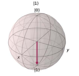
Example 3.1 Let us show that the application of the operator $\sigma_{3}$ (see definition (2.1)) to a qubit in the state $|\psi\rangle=u|0\rangle+v|1\rangle$ brings it to the state $\left|\psi^{\prime}\right\rangle=u|0\rangle-v|1\rangle$.
Proof.
Write a qubit $|\psi\rangle$ in matrix notation:
$$
|\psi\rangle=\left[\begin{array}{l}
u \
v
\end{array}\right] \text {. }
$$
Let us define the action of $\sigma_{3}$ on this quantum state:
$$
\left|\psi^{\prime}\right\rangle=\sigma_{3}\left[\begin{array}{l}
u \
v
\end{array}\right]=\left[\begin{array}{cc}
1 & 0 \
0 & -1
\end{array}\right]\left[\begin{array}{l}
u \
v
\end{array}\right]=\left[\begin{array}{c}
u \
-v
\end{array}\right]=u\left[\begin{array}{l}
1 \
0
\end{array}\right]-v\left[\begin{array}{l}
0 \
1
\end{array}\right]=u|0\rangle-v|1\rangle \text {. }
$$

物理代写|量子计算代写Quantum computer代考|The graphic representation of quantum operations

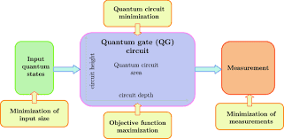
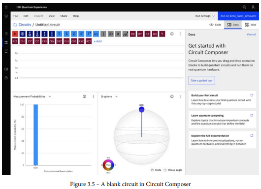
The graphic representation of quantum operations in the form of circuits or diagrams (quantum circuits) is widely used.

A quantum circuit, or network, is an ordered sequence of elements and communication lines connecting them, i.e. wires. Usually, only acyclic circuits are considered in which data flow in one direction-from left to right, and the wires do not return bits to the previous position in the circuit. Input states are attributed to the wires coming from the left. In one time step, each wire may enter data in no more than one gate. The output states are read from the communication lines coming out of the circuit on the right.

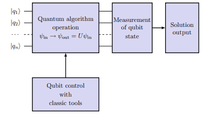
As you can see, the circuit solves a problem of a fixed size. Unlike the quantum circuit, quantum algorithms are defined for input data of any size [5].

A quantum-mechanical operator $U$, which converts a one-qubit gate, is presented as follows:
$$
\left|\psi_{\text {in }}\right\rangle-U
$$
The sequence of the quantum algorithm steps corresponds to the direction on the circuit from left to right.

Table $3.1$ lists the frequently used gates that convert one qubit and the matrix notations of these gates.

Let us show the computation method of the quantum operation matrix based on its effect on basis vectors.
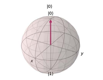
The Hadamard ${ }^{1}$ gate converts the system state in accordance with the rule:
$$
\begin{aligned}
&|0\rangle \rightarrow \frac{1}{\sqrt{2}}(|0\rangle+|1\rangle), \
&|1\rangle \rightarrow \frac{1}{\sqrt{2}}(|0\rangle-|1\rangle) .
\end{aligned}
$$
Consequently, the arbitrary state $|\psi\rangle$ will change in this case as follows:
$$
\begin{aligned}
|\psi\rangle &=\left[\begin{array}{c}
u \
v
\end{array}\right]=u\left[\begin{array}{l}
1 \
0
\end{array}\right]+v\left[\begin{array}{l}
0 \
1
\end{array}\right] \
& \rightarrow u \frac{1}{\sqrt{2}}(|0\rangle+|1\rangle)+v \frac{1}{\sqrt{2}}(|0\rangle-|1\rangle)=\frac{1}{\sqrt{2}}\left[\begin{array}{cc}
1 & 1 \
1 & -1
\end{array}\right]\left[\begin{array}{l}
u \
v
\end{array}\right]
\end{aligned}
$$
Thus, the Hadamard gate, or the Hadamard element, corresponds to the matrix $\frac{1}{\sqrt{2}}\left[\begin{array}{cc}1 & 1 \ 1 & -1\end{array}\right]$.

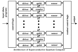
Of course, to execute complex algorithms, the qubits must interact with each other and exchange information. In this regard, logical operations involving two or more qubits are of special importance. In Table $3.2$ are listed the most important gates that transform the state of two qubits.

物理代写|量子计算代写Quantum computer代考|The following quantum state is set

$$
|\psi\rangle=\frac{1}{\sqrt{2}}|0\rangle+\frac{1}{\sqrt{2}} e^{\mathrm{i} \varphi}|1\rangle,
$$
where $\varphi$ is a real number. Let us define the result of measuring this state in bases $B_{1}=$ ${|0\rangle,|1\rangle}$ and $B_{2}={|+\rangle,|-\rangle}$, where $|+\rangle=\frac{1}{2}(|0\rangle+|1\rangle)$ and $|-\rangle=\frac{1}{2}(|0\rangle-|1\rangle)$.
Solution.
First of all, we consider the basis $B_{1}$. According to the measurement postulate (see Appendix A on page 105), the probabilities of getting 0 or 1 as a result of the measurement of the state $u|0\rangle+v|1\rangle$ is equal to $|u|^{2}$ and $|v|^{2}$, respectively. In our example, $u=\frac{1}{\sqrt{2}}$ and $v=\frac{1}{\sqrt{2}} e^{i \varphi}$, therefore the result of the measurement of $M$ is
$$
M=\left{\begin{array}{l}
0 \text { with a probability of } p_{0}=\frac{1}{2}, \
1 \text { with a probability of } p_{1}=\frac{1}{2}
\end{array}\right.
$$
Note that information about the value of $\varphi$ using a measurement in the basis $B_{1}$ cannot be obtained.

Let us turn to measurement using the second basis $B_{2}={|+\rangle,|-\rangle}$. We express the vectors of the computational basis through $|+\rangle$ and $|-\rangle}$ :
$$
\begin{aligned}
|0\rangle &=\frac{1}{\sqrt{2}}(|+\rangle+|-\rangle), \
|1\rangle &=\frac{1}{\sqrt{2}}(|+\rangle+|-\rangle) .
\end{aligned}
$$
In this regard, we obtain
$$
\begin{aligned}
|\psi\rangle &=\frac{1}{\sqrt{2}}|0\rangle+\frac{1}{\sqrt{2}} e^{\mathrm{i} \varphi}|1\rangle \
&=\frac{1}{2}(|+\rangle+|-\rangle)+\frac{1}{2} e^{\mathrm{i} \varphi}(|+\rangle+|-\rangle) \
&=\frac{1}{2}\left(1+e^{\mathrm{i} \varphi}\right)|+\rangle+\frac{1}{2}\left(1-e^{\mathrm{i} \varphi}\right)|-\rangle .
\end{aligned}
$$
The probability of finding the system in the state $|+\rangle$ is
$$
\begin{aligned}
p_{+} &=\frac{1}{2}\left(1+e^{\mathrm{i} \varphi}\right) \times\left(\frac{1}{2}\left(1+e^{\mathrm{i} \varphi}\right)\right)^{*} \
&=\frac{1}{4}\left(1+e^{\mathrm{i} \varphi}\right)\left(1+e^{-\mathrm{i} \varphi}\right)=\frac{1}{4}\left(2+e^{\mathrm{i} \varphi}+e^{-\mathrm{i} \varphi}\right)
\end{aligned}
$$

物理代写|量子计算代写Quantum computer代考|PHYS14

量子计算代考

物理代写|量子计算代写Quantum computer代考|Basic Operations with Qubits

考虑使用量子比特的基本操作。
量子比特上的量子门效应 $|\psi\rangle$ 通过应用量子力学算子发生,例如 $U|\psi\rangle[1-3]$. 运算符可以表示为酉矩阵。特别是, 单个量子比特的演化由大小的酉矩阵描述 $2 \times 2$
多个算子的一致应用 $U_{1}, U_{2}, \ldots, U_{n}$ 一个量子比特相当于某个算子的效果 $W$ 在表格中
$$
W|\psi\rangle=U_{n}\left(U_{n-1}\left(\ldots\left(U_{2}\left(U_{1}|\psi\rangle\right)\right) \ldots\right)\right)=\left(U_{1} U_{2} \ldots U_{n}\right)|\psi\rangle
$$
它的矩阵 $M_{W}$ 是矩阵的乘积 $U_{i}, i=1,2, \ldots, n$ ,以相反的顺序 $[4]$ :
$$
M_{W}=M_{U_{n}} M_{U_{n-1}} \ldots M_{U_{1}} .
$$
这样的运营商 $W$ 被称为算子的乘积 $U_{1}, U_{2}, \ldots, U_{n}$. 由于矩阵乘法运算的不可交换性,应用量子门的顺序通常很 重要。
示例 $3.1$ 让我们展示运算符的应用 $\sigma_{3}$ (见定义 (2.1) ) 到一个量子比特的状态 $|\psi\rangle=u|0\rangle+v|1\rangle$ 把它带到国家 $\left|\psi^{\prime}\right\rangle=u|0\rangle-v|1\rangle$.
证明。
写一个量子位 $|\psi\rangle$ 在矩阵表示法中:
$$
|\psi\rangle=[u v] .
$$
让我们定义 $\sigma_{3}$ 在这个量子态上:
$$
\left|\psi^{\prime}\right\rangle=\sigma_{3}\left[\begin{array}{ll}
u & v
\end{array}\right]=\left[\begin{array}{llll}
1 & 0 & 0 & -1
\end{array}\right]\left[\begin{array}{ll}
u & v
\end{array}\right]=\left[\begin{array}{ll}
u-v
\end{array}\right]=u\left[\begin{array}{ll}
1 & 0
\end{array}\right]-v\left[\begin{array}{ll}
0 & 1
\end{array}\right]=u|0\rangle-v|1\rangle .
$$

物理代写|量子计算代写Quantum computer代考|The graphic representation of quantum operations

以电路或图表(量子电路)形式的量子操作的图形表示被广泛使用。
量子电路或网络是有序的元素序列和连接它们的通信线路,即电线。通常,只考虑非循环电路,其中数据沿一个方 向流动一一从左到右,并且线路不会将位返回到电路中的先前位置。输入状态归因于来自左侧的电线。在一个时间 步长中,每条线可以在不超过一个门中输入数据。输出状态从右侧电路的通信线路中读取。
如您所见,该电路解决了固定尺寸的问题。与量子电路不同,量子算法是为任何大小的输入数据定义的 [5]。
量子力学算子 $U ,$ 它转换一个量子比特门,如下所示:
$$
\left|\psi_{\text {in }}\right\rangle-U
$$
量子算法步骙的顺序对应于电路上从左到右的方向。
桌子 $3.1$ 列出了转换一个量子比特的常用门以及这些门的矩阵符号。
让我们展示基于其对基向量的影响的量子运算矩阵的计算方法。 哈达玛 ${ }^{1}$ Gate 按照规则转换系统状态:
$$
|0\rangle \rightarrow \frac{1}{\sqrt{2}}(|0\rangle+|1\rangle), \quad|1\rangle \rightarrow \frac{1}{\sqrt{2}}(|0\rangle-|1\rangle) .
$$
因此,任意状态 $|\psi\rangle$ 在这种情况下会发生如下变化:
$$
|\psi\rangle=[u v]=u\left[\begin{array}{ll}
1 & 0
\end{array}\right]+v\left[\begin{array}{ll}
0 & 1
\end{array}\right] \quad \rightarrow u \frac{1}{\sqrt{2}}(|0\rangle+|1\rangle)+v \frac{1}{\sqrt{2}}(|0\rangle-|1\rangle)=\frac{1}{\sqrt{2}}\left[\begin{array}{llll}
1 & 1 & -1
\end{array}\right][u v]
$$
因此,Hadamard 门或 Hadamard 元素对应于矩阵 $\frac{1}{\sqrt{2}}\left[\begin{array}{lll}1 & 1 & 1\end{array}\right.$
当然,要执行复杂的算法,量子位必须相互交互并交换信息。在这方面,涉及两个或更多量子位的逻辑操作特别重 要。在表中 $3.2$ 列出了转换两个量子位状态的最重要的门。

物理代写|量子计算代写Quantum computer代考|The following quantum state is set

$$
|\psi\rangle=\frac{1}{\sqrt{2}}|0\rangle+\frac{1}{\sqrt{2}} e^{\mathrm{i} \varphi}|1\rangle
$$
在哪里 $\varphi$ 是一个实数。让我们定义以碱基为单位测量此状态的结果 $B_{1}=|0\rangle,|1\rangle$ 和 $B_{2}=|+\rangle,|-\rangle$ ,在哪里 $|+\rangle=\frac{1}{2}(|0\rangle+|1\rangle)$ 和 $|-\rangle=\frac{1}{2}(|0\rangle-|1\rangle) .$
解决方案。
首先,我们考虑基础 $B_{1}$. 根据测量假设(参见第 105 页的附录 $A$ ),作为状态测量的结果得到 0 或 1 的概率 $u|0\rangle+v|1\rangle$ 等于 $|u|^{2}$ 和 $|v|^{2}$ ,分别。在我们的示例中, $u=\frac{1}{\sqrt{2}}$ 和 $v=\frac{1}{\sqrt{2}} e^{i \varphi}$ ,因此测量的结果 $M$ 是 $\$ \$$
$M=V l e f t{$
0 with a probability of $p_{0}=\frac{1}{2}, 1$ with a probability of $p_{1}=\frac{1}{2}$
正确的。
$\$ \$$
注意关于值的信息 $\varphi$ 在基础中使用测量 $B_{1}$ 无法获得。
让我们转向使用第二个基础进行测量 $B_{2}=|+\rangle,|-\rangle$. 我们通过以下方式表达计算基础的向量 $|+\rangle$ 和 $\mid$ – Irangle} :
$$
|0\rangle=\frac{1}{\sqrt{2}}(|+\rangle+|-\rangle),|1\rangle \quad=\frac{1}{\sqrt{2}}(|+\rangle+|-\rangle) .
$$
在这方面,我们得到
$$
|\psi\rangle=\frac{1}{\sqrt{2}}|0\rangle+\frac{1}{\sqrt{2}} e^{\mathrm{i} \varphi}|1\rangle \quad=\frac{1}{2}(|+\rangle+|-\rangle)+\frac{1}{2} e^{\mathrm{i} \varphi}(|+\rangle+|-\rangle)=\frac{1}{2}\left(1+e^{\mathrm{i} \varphi}\right)|+\rangle+\frac{1}{2}\left(1-e^{\mathrm{i} \varphi}\right)
$$
在该状态下找到系统的概率 $|+\rangle$ 是
$$
p_{+}=\frac{1}{2}\left(1+e^{\mathrm{i} \varphi}\right) \times\left(\frac{1}{2}\left(1+e^{\mathrm{i} \varphi}\right)\right)^{*}=\frac{1}{4}\left(1+e^{\mathrm{i} \varphi}\right)\left(1+e^{-\mathrm{i} \varphi}\right)=\frac{1}{4}\left(2+e^{\mathrm{i} \varphi}+e^{-\mathrm{i} \varphi}\right)
$$

物理代写|量子计算代写Quantum computer代考| 请认准statistics-lab™

统计代写请认准statistics-lab™. statistics-lab™为您的留学生涯保驾护航。

金融工程代写

金融工程是使用数学技术来解决金融问题。金融工程使用计算机科学、统计学、经济学和应用数学领域的工具和知识来解决当前的金融问题,以及设计新的和创新的金融产品。

非参数统计代写

非参数统计指的是一种统计方法,其中不假设数据来自于由少数参数决定的规定模型;这种模型的例子包括正态分布模型和线性回归模型。

广义线性模型代考

广义线性模型(GLM)归属统计学领域,是一种应用灵活的线性回归模型。该模型允许因变量的偏差分布有除了正态分布之外的其它分布。

术语 广义线性模型(GLM)通常是指给定连续和/或分类预测因素的连续响应变量的常规线性回归模型。它包括多元线性回归,以及方差分析和方差分析(仅含固定效应)。

有限元方法代写

有限元方法(FEM)是一种流行的方法,用于数值解决工程和数学建模中出现的微分方程。典型的问题领域包括结构分析、传热、流体流动、质量运输和电磁势等传统领域。

有限元是一种通用的数值方法,用于解决两个或三个空间变量的偏微分方程(即一些边界值问题)。为了解决一个问题,有限元将一个大系统细分为更小、更简单的部分,称为有限元。这是通过在空间维度上的特定空间离散化来实现的,它是通过构建对象的网格来实现的:用于求解的数值域,它有有限数量的点。边界值问题的有限元方法表述最终导致一个代数方程组。该方法在域上对未知函数进行逼近。[1] 然后将模拟这些有限元的简单方程组合成一个更大的方程系统,以模拟整个问题。然后,有限元通过变化微积分使相关的误差函数最小化来逼近一个解决方案。

tatistics-lab作为专业的留学生服务机构,多年来已为美国、英国、加拿大、澳洲等留学热门地的学生提供专业的学术服务,包括但不限于Essay代写,Assignment代写,Dissertation代写,Report代写,小组作业代写,Proposal代写,Paper代写,Presentation代写,计算机作业代写,论文修改和润色,网课代做,exam代考等等。写作范围涵盖高中,本科,研究生等海外留学全阶段,辐射金融,经济学,会计学,审计学,管理学等全球99%专业科目。写作团队既有专业英语母语作者,也有海外名校硕博留学生,每位写作老师都拥有过硬的语言能力,专业的学科背景和学术写作经验。我们承诺100%原创,100%专业,100%准时,100%满意。

随机分析代写


随机微积分是数学的一个分支,对随机过程进行操作。它允许为随机过程的积分定义一个关于随机过程的一致的积分理论。这个领域是由日本数学家伊藤清在第二次世界大战期间创建并开始的。

时间序列分析代写

随机过程,是依赖于参数的一组随机变量的全体,参数通常是时间。 随机变量是随机现象的数量表现,其时间序列是一组按照时间发生先后顺序进行排列的数据点序列。通常一组时间序列的时间间隔为一恒定值(如1秒,5分钟,12小时,7天,1年),因此时间序列可以作为离散时间数据进行分析处理。研究时间序列数据的意义在于现实中,往往需要研究某个事物其随时间发展变化的规律。这就需要通过研究该事物过去发展的历史记录,以得到其自身发展的规律。

回归分析代写

多元回归分析渐进(Multiple Regression Analysis Asymptotics)属于计量经济学领域,主要是一种数学上的统计分析方法,可以分析复杂情况下各影响因素的数学关系,在自然科学、社会和经济学等多个领域内应用广泛。

MATLAB代写

MATLAB 是一种用于技术计算的高性能语言。它将计算、可视化和编程集成在一个易于使用的环境中,其中问题和解决方案以熟悉的数学符号表示。典型用途包括:数学和计算算法开发建模、仿真和原型制作数据分析、探索和可视化科学和工程图形应用程序开发,包括图形用户界面构建MATLAB 是一个交互式系统,其基本数据元素是一个不需要维度的数组。这使您可以解决许多技术计算问题,尤其是那些具有矩阵和向量公式的问题,而只需用 C 或 Fortran 等标量非交互式语言编写程序所需的时间的一小部分。MATLAB 名称代表矩阵实验室。MATLAB 最初的编写目的是提供对由 LINPACK 和 EISPACK 项目开发的矩阵软件的轻松访问,这两个项目共同代表了矩阵计算软件的最新技术。MATLAB 经过多年的发展,得到了许多用户的投入。在大学环境中,它是数学、工程和科学入门和高级课程的标准教学工具。在工业领域,MATLAB 是高效研究、开发和分析的首选工具。MATLAB 具有一系列称为工具箱的特定于应用程序的解决方案。对于大多数 MATLAB 用户来说非常重要,工具箱允许您学习应用专业技术。工具箱是 MATLAB 函数(M 文件)的综合集合,可扩展 MATLAB 环境以解决特定类别的问题。可用工具箱的领域包括信号处理、控制系统、神经网络、模糊逻辑、小波、仿真等。

R语言代写问卷设计与分析代写
PYTHON代写回归分析与线性模型代写
MATLAB代写方差分析与试验设计代写
STATA代写机器学习/统计学习代写
SPSS代写计量经济学代写
EVIEWS代写时间序列分析代写
EXCEL代写深度学习代写
SQL代写各种数据建模与可视化代写

物理代写|量子计算代写Quantum computer代考|CS583

如果你也在 怎样代写量子计算Quantum computer这个学科遇到相关的难题,请随时右上角联系我们的24/7代写客服。

量子计算机是利用量子物理学的特性来存储数据和进行计算的机器。这对于某些任务来说是非常有利的,它们甚至可以大大超过我们最好的超级计算机。

statistics-lab™ 为您的留学生涯保驾护航 在代写量子计算Quantum computer方面已经树立了自己的口碑, 保证靠谱, 高质且原创的统计Statistics代写服务。我们的专家在代写量子计算Quantum computer代写方面经验极为丰富,各种代写量子计算Quantum computer相关的作业也就用不着说。

我们提供的量子计算Quantum computer及其相关学科的代写,服务范围广, 其中包括但不限于:

  • Statistical Inference 统计推断
  • Statistical Computing 统计计算
  • Advanced Probability Theory 高等概率论
  • Advanced Mathematical Statistics 高等数理统计学
  • (Generalized) Linear Models 广义线性模型
  • Statistical Machine Learning 统计机器学习
  • Longitudinal Data Analysis 纵向数据分析
  • Foundations of Data Science 数据科学基础
物理代写|量子计算代写Quantum computer代考|CS583

物理代写|量子计算代写Quantum computer代考|Pauli Matrices and Dirac Matrices

For the imaginary unit $\sqrt{-1}$, we will use the designation $i \equiv \sqrt{-1}$. The matrices $\sigma_{1}, \sigma_{2}$, and $\sigma_{3}$ :
$$
\sigma_{1}=\left[\begin{array}{ll}
0 & 1 \
1 & 0
\end{array}\right], \quad \sigma_{2}=\left[\begin{array}{cc}
0 & -\mathrm{i} \
\mathrm{i} & 0
\end{array}\right], \quad \sigma_{3}=\left[\begin{array}{cc}
1 & 0 \
0 & -1
\end{array}\right],
$$
are called the Pauli matrices. They are widely used in quantum theory for describing half-integer spin particles, for example, an electron. (Spin is a quantum property of an elementary particle, its intrinsic angular momentum [1]. So, electrons, protons, and neutrinos have half-integer spin; the spin of photons and gravitons is an integer.).
The following properties are valid for the Pauli matrices.
(1) The Pauli matrices are Hermitian ${ }^{1}$ and unitary (see Appendix B on page 103):
$$
\forall k \in{1,2,3} \quad \sigma_{k}=\sigma_{k}^{\dagger}=\sigma_{k}^{-1} .
$$
(2) $\forall k \in{1,2,3}$, the square of the Pauli matrix is equal to the identity matrix:
$$
\sigma_{i}^{2}=\left[\begin{array}{ll}
1 & 0 \
0 & 1
\end{array}\right]
$$
(3) $\forall i, j \in{1,2,3}$, the equalities
$$
\sigma_{i} \sigma_{j}+\sigma_{j} \sigma_{i}=2 \delta_{i j}\left[\begin{array}{ll}
1 & 0 \
0 & 1
\end{array}\right]
$$
are valid. Here, is used a notation for the Kronecker symbol (see definition on page 3 ).
Note that the value ${A, B}=A B+B A$ is usually called anticommutator of matrices $A$ and $B$, and the value $[A, B]=A B-B A$ is called commutator. Next,for the identity matrix, we will apply the notation $I$, and for the zero one $O$. In particular, the formula (2.4) can be written as follows:
$$
\left{\sigma_{i}, \sigma_{j}\right}=2 \delta_{i j} I .
$$
The matrices $A$ and $B$ are called commutative, if $A B=B A$. Commutative matrices are always square and have the same order.

By definition, the condition $[A, B]=O$ is met for the commutative matrices [2]. It is clear that the Pauli matrices do not commutate with each other (see Exercise 1).

物理代写|量子计算代写Quantum computer代考|Let us prove the Jacobi2 identity

$$
[[P, Q], R]+[[Q, R], P]+[[R, P], Q] \equiv O
$$
that is valid for commutators of any matrices of size $n \times n$.
Proof.
We use the definition of the commutator $[P, Q]=P Q-Q P$, then
$$
\begin{aligned}
{[[P, Q], R] } &=[P Q-Q P, R]=(P Q-Q P) R-R(P Q-Q P) \
&=P Q R-Q P R-R P Q+R Q P
\end{aligned}
$$
Next, let us present in a similar manner the remaining summands in the sum:
$$
\begin{aligned}
&{[[Q, R], P]=Q R P-R Q P-P Q R+P R Q} \
&{[[R, P], Q]=R P Q-P R Q-Q R P+Q P R .}
\end{aligned}
$$
The sum of right-hand values (2.7), (2.8), and (2.9), as can be easily seen after the conversion of such summands, is zero. In this way, the Jacobi identity is proved.
Sometimes, in linear algebra and its applications, one has to use matrices split into rectangular parts or blocks [3,4]. Consider the rectangular matrix $A=\left(a_{i j}\right)$, where $1 \leqslant i \leqslant m, 1 \leqslant j \leqslant n$. Let $m=m_{1}+m_{2}$ and $n=n_{1}+n_{2}$.

Let us draw horizontal and vertical lines and split the matrix $A$ into four rectangular blocks:Thus, the matrix $A$ is presented in the form of a block matrix, consisting of the blocks $B_{11}, B_{12}, B_{21}$, and $B_{22}$ of size $m_{1} \times n_{1}, m_{1} \times n_{2}, m_{2} \times n_{1}$, and $m_{2} \times n_{2}$, respectively.

物理代写|量子计算代写Quantum computer代考|Dirac matrices

As an example of a block matrix setting, we provide the definition of the Dirac matrices. Four Dirac matrices $\alpha_{1}, \alpha_{2}, \alpha_{3}$, and $\beta$ are part of the equation named after him for a half-integer spin relativistic particle, and are expressed in terms of the Pauli matrices $\sigma_{k}, k=1,2,3$, as follows [5]:
$$
\alpha_{k}=\left[\begin{array}{cc}
O & \sigma_{k} \
\sigma_{k} & O
\end{array}\right], \quad \beta=\left[\begin{array}{cc}
I & O \
O & -I
\end{array}\right]
$$
(Relativistic particles are the particles whose velocity is close to the velocity of light.)
Each of the Dirac matrices has a Hermitian property and a property of being unitary. Moreover, for all $l, m \in{1,2,3}$ the equalities
$$
\begin{aligned}
\alpha_{l} \alpha_{m}+\alpha_{m} \alpha_{l} &=2 \delta_{l m} I, \
\alpha_{l} \beta+\beta \alpha_{l} &=O
\end{aligned}
$$
are valid. Note that the size of matrices $I$ and $O$ in formulas (2.12) and (2.13) is equal to $4 \times 4$.

Using the concept of a block matrix, it is easy to write down the definition of the tensor product of square matrices $A \otimes B$, defined as $A=\left(a_{i j}\right), i, j=1,2, \ldots, n_{A}$, and $B=\left(b_{i j}\right), i, j=1,2, \ldots, n_{B}$ :
$$
A \otimes B=\left[\begin{array}{cccc}
a_{11} B & a_{12} B & \ldots & a_{1 n_{A}} B \
a_{21} B & a_{22} B & \ldots & a_{2 n_{A}} B \
\vdots & \vdots & \ddots & \vdots \
a_{n_{A} 1} B & a_{n_{A} 2} B & \ldots & a_{n_{A} n_{A}} B
\end{array}\right]
$$
where $a_{11} B$ is a block with size $n_{B} \times n_{B}$, consisting of elements of the form $a_{11} b_{i j}$, block $a_{12} B$ consists of elements of the form $a_{12} b_{i j}$, etc.

Note that for the tensor product operation, the sizes of matrices $A$ and $B$ do not have to be the same, i.e. $n_{A} \neq n_{B}$.

物理代写|量子计算代写Quantum computer代考|CS583

量子计算代考

物理代写|量子计算代写Quantum computer代考|Pauli Matrices and Dirac Matrices

对于虚数单位−1, 我们将使用名称一世≡−1. 矩阵σ1,σ2, 和σ3 :

σ1=[01 10],σ2=[0−一世 一世0],σ3=[10 0−1],
称为泡利矩阵。它们在量子理论中被广泛用于描述半整数自旋粒子,例如电子。(自旋是基本粒子的一种量子特性,它的固有角动量 [1]。因此,电子、质子和中微子具有半整数自旋;光子和引力子的自旋是整数。)。
以下性质对泡利矩阵有效。
(1) Pauli 矩阵是 Hermitian 矩阵1和单一的(参见第 103 页的附录 B):

∀ķ∈1,2,3σķ=σķ†=σķ−1.
(2) ∀ķ∈1,2,3,泡利矩阵的平方等于单位矩阵:

σ一世2=[10 01]
(3) ∀一世,j∈1,2,3, 等式

σ一世σj+σjσ一世=2d一世j[10 01]
是有效的。在这里,使用了克罗内克符号的符号(参见第 3 页的定义)。
请注意,该值一个,乙=一个乙+乙一个通常称为矩阵的反对易子一个和乙, 和值[一个,乙]=一个乙−乙一个称为换向器。接下来,对于单位矩阵,我们将应用符号我,对于零一○. 特别地,公式(2.4)可以写成:

\left{\sigma_{i}, \sigma_{j}\right}=2 \delta_{i j} I 。\left{\sigma_{i}, \sigma_{j}\right}=2 \delta_{i j} I 。
矩阵一个和乙被称为可交换的,如果一个乙=乙一个. 交换矩阵总是方阵并且具有相同的阶。

根据定义,条件[一个,乙]=○满足交换矩阵[2]。很明显,泡利矩阵不会相互交换(参见练习 1)。

物理代写|量子计算代写Quantum computer代考|Let us prove the Jacobi2 identity

$$
[[P, Q], R]+[[Q, R], P]+[[R, P], Q] \equiv O
$$
这对任何大小矩阵的交换器都有效 $n \times n$.
证明。
我们使用换向器的定义 $[P, Q]=P Q-Q P$ ,然后
$$
[[P, Q], R]=[P Q-Q P, R]=(P Q-Q P) R-R(P Q-Q P) \quad=P Q R-Q P R-R P Q+R Q P
$$
接下来,让我们以类似的方式呈现 sum 中的剩余加数:
$$
[[Q, R], P]=Q R P-R Q P-P Q R+P R Q \quad[[R, P], Q]=R P Q-P R Q-Q R P+Q P R
$$
右手边的值 (2.7)、(2.8) 和 (2.9) 之和,在这些和数的转换之后可以很容易地看出,为零。这样就证明了Jacobi 恒 等式边。
有时,在线性代数及其应用中,必须使用分割成矩形部分或块的矩阵 $[3,4]$ 。考虑矩形矩阵 $A=\left(a_{i j}\right)$ ,在哪里 $1 \leqslant i \leqslant m, 1 \leqslant j \leqslant n$. 让 $m=m_{1}+m_{2}$ 和 $n=n_{1}+n_{2}$.
让我们绘制水平和垂直线并拆分矩阵 $A$ 分成四个矩形块:因此,矩阵 $A$ 以块矩阵的形式呈现,由块组成 $B_{11}, B_{12}, B_{21}$ ,和 $B_{22}$ 大小的 $m_{1} \times n_{1}, m_{1} \times n_{2}, m_{2} \times n_{1}$ ,和 $m_{2} \times n_{2}$ ,分别。

物理代写|量子计算代写Quantum computer代考|Dirac matrices

作为块矩阵设置的示例,我们提供了狄拉克矩阵的定义。四个狄拉克矩阵 $\alpha_{1}, \alpha_{2}, \alpha_{3}$ ,和 $\beta$ 是半整数自旋相对论粒 子方程的一部分,并用泡利矩阵表示 $\sigma_{k}, k=1,2,3 ,$ 如下[5]:
(相对论粒子是速度接近光速的粒子。)
每个狄拉克矩阵都具有厄米特性质和西性质。此外,对于所有 $l, m \in 1,2,3$ 平等
$$
\alpha_{l} \alpha_{m}+\alpha_{m} \alpha_{l}=2 \delta_{l m} I, \alpha_{l} \beta+\beta \alpha_{l} \quad=O
$$
是有效的。注意矩阵的大小 $I$ 和 $O$ 在公式 (2.12) 和 (2.13) 中等于 $4 \times 4$.
使用块矩阵的概念,很容易写出方阵张量积的定义 $A \otimes B$ ,定义为 $A=\left(a_{i j}\right), i, j=1,2, \ldots, n_{A}$ ,和 $B=\left(b_{i j}\right), i, j=1,2, \ldots, n_{B}$ :
$A \otimes B=\left[\begin{array}{lllllllllll}a_{11} B & a_{12} B & \ldots & a_{1 n_{A}} B & a_{21} B & a_{22} B & \ldots & a_{2 n_{A}} B & \vdots & \ddots & \vdots a_{n_{A} 1} B\end{array}\right.$
在哪里 $a_{11} B$ 是一个有大小的块 $n_{B} \times n_{B}$ ,由形式的元素组成 $a_{11} b_{i j}$ ,堵塞 $a_{12} B$ 由表单元素组成 $a_{12} b_{i j} , E T C$ 。
请注意,对于张量积运算,矩阵的大小 $A$ 和 $B$ 不必相同,即 $n_{A} \neq n_{B}$.

物理代写|量子计算代写Quantum computer代考| 请认准statistics-lab™

统计代写请认准statistics-lab™. statistics-lab™为您的留学生涯保驾护航。

金融工程代写

金融工程是使用数学技术来解决金融问题。金融工程使用计算机科学、统计学、经济学和应用数学领域的工具和知识来解决当前的金融问题,以及设计新的和创新的金融产品。

非参数统计代写

非参数统计指的是一种统计方法,其中不假设数据来自于由少数参数决定的规定模型;这种模型的例子包括正态分布模型和线性回归模型。

广义线性模型代考

广义线性模型(GLM)归属统计学领域,是一种应用灵活的线性回归模型。该模型允许因变量的偏差分布有除了正态分布之外的其它分布。

术语 广义线性模型(GLM)通常是指给定连续和/或分类预测因素的连续响应变量的常规线性回归模型。它包括多元线性回归,以及方差分析和方差分析(仅含固定效应)。

有限元方法代写

有限元方法(FEM)是一种流行的方法,用于数值解决工程和数学建模中出现的微分方程。典型的问题领域包括结构分析、传热、流体流动、质量运输和电磁势等传统领域。

有限元是一种通用的数值方法,用于解决两个或三个空间变量的偏微分方程(即一些边界值问题)。为了解决一个问题,有限元将一个大系统细分为更小、更简单的部分,称为有限元。这是通过在空间维度上的特定空间离散化来实现的,它是通过构建对象的网格来实现的:用于求解的数值域,它有有限数量的点。边界值问题的有限元方法表述最终导致一个代数方程组。该方法在域上对未知函数进行逼近。[1] 然后将模拟这些有限元的简单方程组合成一个更大的方程系统,以模拟整个问题。然后,有限元通过变化微积分使相关的误差函数最小化来逼近一个解决方案。

tatistics-lab作为专业的留学生服务机构,多年来已为美国、英国、加拿大、澳洲等留学热门地的学生提供专业的学术服务,包括但不限于Essay代写,Assignment代写,Dissertation代写,Report代写,小组作业代写,Proposal代写,Paper代写,Presentation代写,计算机作业代写,论文修改和润色,网课代做,exam代考等等。写作范围涵盖高中,本科,研究生等海外留学全阶段,辐射金融,经济学,会计学,审计学,管理学等全球99%专业科目。写作团队既有专业英语母语作者,也有海外名校硕博留学生,每位写作老师都拥有过硬的语言能力,专业的学科背景和学术写作经验。我们承诺100%原创,100%专业,100%准时,100%满意。

随机分析代写


随机微积分是数学的一个分支,对随机过程进行操作。它允许为随机过程的积分定义一个关于随机过程的一致的积分理论。这个领域是由日本数学家伊藤清在第二次世界大战期间创建并开始的。

时间序列分析代写

随机过程,是依赖于参数的一组随机变量的全体,参数通常是时间。 随机变量是随机现象的数量表现,其时间序列是一组按照时间发生先后顺序进行排列的数据点序列。通常一组时间序列的时间间隔为一恒定值(如1秒,5分钟,12小时,7天,1年),因此时间序列可以作为离散时间数据进行分析处理。研究时间序列数据的意义在于现实中,往往需要研究某个事物其随时间发展变化的规律。这就需要通过研究该事物过去发展的历史记录,以得到其自身发展的规律。

回归分析代写

多元回归分析渐进(Multiple Regression Analysis Asymptotics)属于计量经济学领域,主要是一种数学上的统计分析方法,可以分析复杂情况下各影响因素的数学关系,在自然科学、社会和经济学等多个领域内应用广泛。

MATLAB代写

MATLAB 是一种用于技术计算的高性能语言。它将计算、可视化和编程集成在一个易于使用的环境中,其中问题和解决方案以熟悉的数学符号表示。典型用途包括:数学和计算算法开发建模、仿真和原型制作数据分析、探索和可视化科学和工程图形应用程序开发,包括图形用户界面构建MATLAB 是一个交互式系统,其基本数据元素是一个不需要维度的数组。这使您可以解决许多技术计算问题,尤其是那些具有矩阵和向量公式的问题,而只需用 C 或 Fortran 等标量非交互式语言编写程序所需的时间的一小部分。MATLAB 名称代表矩阵实验室。MATLAB 最初的编写目的是提供对由 LINPACK 和 EISPACK 项目开发的矩阵软件的轻松访问,这两个项目共同代表了矩阵计算软件的最新技术。MATLAB 经过多年的发展,得到了许多用户的投入。在大学环境中,它是数学、工程和科学入门和高级课程的标准教学工具。在工业领域,MATLAB 是高效研究、开发和分析的首选工具。MATLAB 具有一系列称为工具箱的特定于应用程序的解决方案。对于大多数 MATLAB 用户来说非常重要,工具箱允许您学习应用专业技术。工具箱是 MATLAB 函数(M 文件)的综合集合,可扩展 MATLAB 环境以解决特定类别的问题。可用工具箱的领域包括信号处理、控制系统、神经网络、模糊逻辑、小波、仿真等。

R语言代写问卷设计与分析代写
PYTHON代写回归分析与线性模型代写
MATLAB代写方差分析与试验设计代写
STATA代写机器学习/统计学习代写
SPSS代写计量经济学代写
EVIEWS代写时间序列分析代写
EXCEL代写深度学习代写
SQL代写各种数据建模与可视化代写

物理代写|量子计算代写Quantum computer代考|Physics 421

如果你也在 怎样代写量子计算Quantum computer这个学科遇到相关的难题,请随时右上角联系我们的24/7代写客服。

量子计算机是利用量子物理学的特性来存储数据和进行计算的机器。这对于某些任务来说是非常有利的,它们甚至可以大大超过我们最好的超级计算机。

statistics-lab™ 为您的留学生涯保驾护航 在代写量子计算Quantum computer方面已经树立了自己的口碑, 保证靠谱, 高质且原创的统计Statistics代写服务。我们的专家在代写量子计算Quantum computer代写方面经验极为丰富,各种代写量子计算Quantum computer相关的作业也就用不着说。

我们提供的量子计算Quantum computer及其相关学科的代写,服务范围广, 其中包括但不限于:

  • Statistical Inference 统计推断
  • Statistical Computing 统计计算
  • Advanced Probability Theory 高等概率论
  • Advanced Mathematical Statistics 高等数理统计学
  • (Generalized) Linear Models 广义线性模型
  • Statistical Machine Learning 统计机器学习
  • Longitudinal Data Analysis 纵向数据分析
  • Foundations of Data Science 数据科学基础
物理代写|量子计算代写Quantum computer代考|Physics 421

物理代写|量子计算代写Quantum computer代考|Quantum Computing Model

Quantum computers use processes of a quantum nature manifested with atoms, molecules, molecular clusters, etc. The description of such processes is based on the application of complex numbers and complex matrices.

As is well known, the basic notion of classical information theory is a bit [1]. A classical bit takes the values 0 or 1 (and no other).

A qubit (quantum bit) is the smallest element that executes the information storage function in a quantum computer [2].

Qubit is a quantum system $|\psi\rangle$ that allows two states: $|0\rangle$ and $|1\rangle$. In accordance with the so-called “bra-ket” Dirac ” notation (from word bra(c)ket), the symbols $\mid 0$ ) and $|1\rangle$ are read as “Ket $0 “$ and “Ket 1 “, respectively. The brackets $|. .\rangle\rangle$ show that $\psi$ is some state of the quantum system.

The fundamental difference between the classical bit and the qubit consists in that, the qubit can be in a state different from $|0\rangle$ or $|1\rangle$. The arbitrary state of the qubit is defined by the linear combination of basis states:
$$
|\psi\rangle=u|0\rangle+v|1\rangle,
$$
where the complex coefficients $u$ and $v$ satisfy the following normalization condition:
$$
|u|^{2}+|v|^{2}=1 .
$$
The mathematical description of basis states reduces to their representation in matrix form:
$$
|0\rangle=\left[\begin{array}{l}
1 \
0
\end{array}\right], \quad|1\rangle=\left[\begin{array}{l}
0 \
1
\end{array}\right]
$$
Based on the presentation (1.3), the arbitrary state of the qubit is written as
$$
|\psi\rangle=\left[\begin{array}{l}
u \
v
\end{array}\right]
$$

物理代写|量子计算代写Quantum computer代考|The orthogonality condition

The orthogonality condition of two states $\left|\psi^{\prime}\right\rangle$ and $\left|\psi^{\prime \prime}\right\rangle$ is written as follows:
$$
\left\langle\psi^{\prime} \mid \psi^{\prime \prime}\right\rangle=\sum_{i=1}^{2^{n}} u_{i}^{*} v_{i}=0 .
$$
Note that the states of the computational base (1.6) are orthonormalized.
To change the state of a quantum system, quantum operations are used, which are called quantum logic gates, or, for short, simply gates. Thus, gates perform logical operations on qubits. Note that the change of state $|\psi\rangle$ in time is also referred to as the evolution of the quantum system.

An important step of quantum algorithms is the procedure of measurement of a state. When the qubit state is measured, it randomly passes to one of its states: $|0\rangle$ or $|1\rangle$. Therefore, the complex coefficients $u$ and $v$ from the qubit definition (1.1) are associated with the probability to get the value 0 or 1 when its state is measured. According to the postulates of quantum theory, the probabilities of passing to the states $|0\rangle$ and $|1\rangle$ are equal to $|u|^{2}$ and $|v|^{2}$, respectively. In this connection, the equality (1.2) reflects the probability conservation law. After the measurement, the qubit passes to the basis state, complying with the classical result of the measurement. Generally speaking, the probabilities of getting the result 0 and 1 are different for different states of the quantum system.

In other words, quantum computing is a sequence of simple form operations with the collection of the interacting qubits. In the final step of the quantum computing procedure, the state of the quantum system is measured and a conclusion about the computing result is made. The measurement makes it possible to obtain, at a macroscopic level, the information about the quantum state. The peculiarity of the quantum measurements is their irreversibility, which radically differentiates quantum computing from the classical one.

Despite the fact that the number of qubit states is infinite, with the help of measurement it is possible to obtain only one bit of classical information. The measurement procedure transfers the qubit state to one of the basis states, so a second measurement will produce the same result.

Quantum computer is a set of $n$ qubits controlled by external (classic) signals [812]. Often, an ordered set of some qubits is called a register. The main elements of a quantum computer are shown in Fig. 1.1.

The classical quantum computer setting consists of the controlling classical computer and impulse generators controlling the qubit evolution, as well as measurement instruments of the qubit state. The system from $n$ qubits in the initial state, e.g. $\left|\psi_{\text {in }}\right\rangle=|00 \ldots 0\rangle$, forms a memory register prepared to record input data and perform computations. The data are recorded by an external action on each of the system’s qubits. The solution of the problem is determined by a measurement of the final state qubits $\left|\psi_{\text {out }}\right\rangle[2,12]$.

物理代写|量子计算代写Quantum computer代考|Main elements of a quantum computer

In this record, the state $|\psi\rangle$ of the $n$-qubit register of a quantum computer is expressed through the superposition of vectors of computational basis $B={|0\rangle,|1\rangle, \ldots$, $\left.\left|2^{n}-1\right\rangle\right}$ by the formula
$$
|\psi\rangle=\sum_{k=0}^{2^{n}-1} c_{k}|k\rangle
$$
where the normalization condition
$$
\sum_{k=0}^{2^{k}-1}\left|c_{k}\right|^{2}=1
$$
is met.
A quantum system, formed by $N$ two-level elements, has $\Sigma(N)=2^{N}$ independent states. The key point of the functioning of such a system is the interaction of separate qubits with each other. The number of states $\Sigma(N)$ grows exponentially with the growth of the quantum system, which allows solving practical problems of a very high asymptotic complexity. For example, an efficient quantum algorithm of prime factorization is known, which is very important for cryptography [13]. As a result, the quantum algorithms provide exponential or polynomial speedup in comparison with the classical solution methods for many problems.

Unfortunately, no full-function quantum computer has been created yet, although many of its elements have already been built and studied at the world’s leading laboratories $[11,14,15]$. The main obstacle to the development of quantum computing is the instability of a system of many qubits. The more the qubits are united into an entangled system, the more the effort is required to ensure the smallness of the number of measurement errors. Nevertheless, the history of quantum computer development demonstrates an enormous potential laid in the uniting of quantum theory and algorithm theory.

物理代写|量子计算代写Quantum computer代考|Physics 421

量子计算代考

物理代写|量子计算代写Quantum computer代考|Quantum Computing Model

量子计算机使用具有原子、分子、分子簇等的量子性质的过程。对这些过程的描述是基于复数和复矩阵的应用。

众所周知,经典信息论的基本概念有点[1]。经典位采用值 0 或 1(没有其他值)。

qubit(量子位)是量子计算机中执行信息存储功能的最小元素[2]。

Qubit是一个量子系统|ψ⟩允许两种状态:|0⟩和|1⟩. 根据所谓的“bra-ket”狄拉克“符号(来自单词 bra(c)ket),符号∣0) 和|1⟩读作“凯0“和“Ket 1”,分别。括号|..⟩⟩显示ψ是量子系统的某种状态。

经典比特和量子比特之间的根本区别在于,量子比特可以处于不同于|0⟩或者|1⟩. 量子比特的任意状态由基态的线性组合定义:

|ψ⟩=在|0⟩+在|1⟩,
其中复系数在和在满足以下归一化条件:

|在|2+|在|2=1.
基态的数学描述简化为矩阵形式的表示:

|0⟩=[1 0],|1⟩=[0 1]
根据介绍(1.3),量子位的任意状态写为

|ψ⟩=[在 在]

物理代写|量子计算代写Quantum computer代考|The orthogonality condition

两个状态的正交性条件|ψ′⟩和|ψ′′⟩写成如下:

⟨ψ′∣ψ′′⟩=∑一世=12n在一世∗在一世=0.
请注意,计算基 (1.6) 的状态是正交归一化的。
为了改变量子系统的状态,使用了量子操作,称为量子逻辑门,或者简称为门。因此,门对量子位执行逻辑运算。注意状态的变化|ψ⟩在时间上也被称为量子系统的演化。

量子算法的一个重要步骤是测量状态的过程。当测量量子比特状态时,它会随机进入其状态之一:|0⟩或者|1⟩. 因此,复系数在和在从量子比特定义 (1.1) 中,当测量其状态时,它与获得值 0 或 1 的概率相关联。根据量子理论的假设,传递到状态的概率|0⟩和|1⟩等于|在|2和|在|2, 分别。在这方面,等式(1.2)反映了概率守恒定律。测量后,量子比特进入基态,符合经典的测量结果。一般来说,对于量子系统的不同状态,得到结果 0 和 1 的概率是不同的。

换句话说,量子计算是一系列简单形式的操作,其中包含相互作用的量子比特的集合。在量子计算过程的最后一步,测量量子系统的状态并得出计算结果的结论。测量可以在宏观水平上获得有关量子态的信息。量子测量的特点是它们的不可逆性,这从根本上将量子计算与经典计算区分开来。

尽管量子比特状态的数量是无限的,但在测量的帮助下,可能只获得一位经典信息。测量过程将量子位状态转移到一个基本状态,因此第二次测量将产生相同的结果。

量子计算机是一组n由外部(经典)信号控制的量子比特[812]。通常,一组有序的一些量子比特称为寄存器。量子计算机的主要元件如图 1.1 所示。

经典量子计算机设置包括控制经典计算机和控制量子比特演化的脉冲发生器,以及量子比特状态的测量仪器。该系统从n初始状态的量子比特,例如|ψ在 ⟩=|00…0⟩,形成一个准备记录输入数据和执行计算的内存寄存器。数据是通过对系统的每个量子位进行外部操作来记录的。问题的解决方案由最终状态量子比特的测量决定|ψ出去 ⟩[2,12].

物理代写|量子计算代写Quantum computer代考|Main elements of a quantum computer

在该记录中,该州|ψ⟩的n-量子计算机的qubit寄存器通过计算基向量的叠加来表示B={|0\rangle,|1\rangle, \ldots$, $\left.\left|2^{n}-1\right\rangle\right}B={|0\rangle,|1\rangle, \ldots$, $\left.\left|2^{n}-1\right\rangle\right}由公式

|ψ⟩=∑ķ=02n−1Cķ|ķ⟩
其中归一化条件

∑ķ=02ķ−1|Cķ|2=1
满足。
一个量子系统,由ñ两级元素,有Σ(ñ)=2ñ独立国家。这种系统运行的关键是不同量子位之间的相互作用。状态数Σ(ñ)随着量子系统的增长呈指数增长,这允许解决具有非常高渐近复杂度的实际问题。例如,已知一种有效的素因数分解量子算法,这对密码学非常重要[13]。因此,与许多问题的经典求解方法相比,量子算法提供了指数或多项式加速。

不幸的是,尚未创建全功能的量子计算机,尽管它的许多元素已经在世界领先的实验室建造和研究[11,14,15]. 量子计算发展的主要障碍是多量子比特系统的不稳定性。量子比特越多地结合成一个纠缠系统,就越需要努力确保测量误差的数量很小。尽管如此,量子计算机发展的历史证明了量子理论和算法理论结合的巨大潜力。

物理代写|量子计算代写Quantum computer代考| 请认准statistics-lab™

统计代写请认准statistics-lab™. statistics-lab™为您的留学生涯保驾护航。

金融工程代写

金融工程是使用数学技术来解决金融问题。金融工程使用计算机科学、统计学、经济学和应用数学领域的工具和知识来解决当前的金融问题,以及设计新的和创新的金融产品。

非参数统计代写

非参数统计指的是一种统计方法,其中不假设数据来自于由少数参数决定的规定模型;这种模型的例子包括正态分布模型和线性回归模型。

广义线性模型代考

广义线性模型(GLM)归属统计学领域,是一种应用灵活的线性回归模型。该模型允许因变量的偏差分布有除了正态分布之外的其它分布。

术语 广义线性模型(GLM)通常是指给定连续和/或分类预测因素的连续响应变量的常规线性回归模型。它包括多元线性回归,以及方差分析和方差分析(仅含固定效应)。

有限元方法代写

有限元方法(FEM)是一种流行的方法,用于数值解决工程和数学建模中出现的微分方程。典型的问题领域包括结构分析、传热、流体流动、质量运输和电磁势等传统领域。

有限元是一种通用的数值方法,用于解决两个或三个空间变量的偏微分方程(即一些边界值问题)。为了解决一个问题,有限元将一个大系统细分为更小、更简单的部分,称为有限元。这是通过在空间维度上的特定空间离散化来实现的,它是通过构建对象的网格来实现的:用于求解的数值域,它有有限数量的点。边界值问题的有限元方法表述最终导致一个代数方程组。该方法在域上对未知函数进行逼近。[1] 然后将模拟这些有限元的简单方程组合成一个更大的方程系统,以模拟整个问题。然后,有限元通过变化微积分使相关的误差函数最小化来逼近一个解决方案。

tatistics-lab作为专业的留学生服务机构,多年来已为美国、英国、加拿大、澳洲等留学热门地的学生提供专业的学术服务,包括但不限于Essay代写,Assignment代写,Dissertation代写,Report代写,小组作业代写,Proposal代写,Paper代写,Presentation代写,计算机作业代写,论文修改和润色,网课代做,exam代考等等。写作范围涵盖高中,本科,研究生等海外留学全阶段,辐射金融,经济学,会计学,审计学,管理学等全球99%专业科目。写作团队既有专业英语母语作者,也有海外名校硕博留学生,每位写作老师都拥有过硬的语言能力,专业的学科背景和学术写作经验。我们承诺100%原创,100%专业,100%准时,100%满意。

随机分析代写


随机微积分是数学的一个分支,对随机过程进行操作。它允许为随机过程的积分定义一个关于随机过程的一致的积分理论。这个领域是由日本数学家伊藤清在第二次世界大战期间创建并开始的。

时间序列分析代写

随机过程,是依赖于参数的一组随机变量的全体,参数通常是时间。 随机变量是随机现象的数量表现,其时间序列是一组按照时间发生先后顺序进行排列的数据点序列。通常一组时间序列的时间间隔为一恒定值(如1秒,5分钟,12小时,7天,1年),因此时间序列可以作为离散时间数据进行分析处理。研究时间序列数据的意义在于现实中,往往需要研究某个事物其随时间发展变化的规律。这就需要通过研究该事物过去发展的历史记录,以得到其自身发展的规律。

回归分析代写

多元回归分析渐进(Multiple Regression Analysis Asymptotics)属于计量经济学领域,主要是一种数学上的统计分析方法,可以分析复杂情况下各影响因素的数学关系,在自然科学、社会和经济学等多个领域内应用广泛。

MATLAB代写

MATLAB 是一种用于技术计算的高性能语言。它将计算、可视化和编程集成在一个易于使用的环境中,其中问题和解决方案以熟悉的数学符号表示。典型用途包括:数学和计算算法开发建模、仿真和原型制作数据分析、探索和可视化科学和工程图形应用程序开发,包括图形用户界面构建MATLAB 是一个交互式系统,其基本数据元素是一个不需要维度的数组。这使您可以解决许多技术计算问题,尤其是那些具有矩阵和向量公式的问题,而只需用 C 或 Fortran 等标量非交互式语言编写程序所需的时间的一小部分。MATLAB 名称代表矩阵实验室。MATLAB 最初的编写目的是提供对由 LINPACK 和 EISPACK 项目开发的矩阵软件的轻松访问,这两个项目共同代表了矩阵计算软件的最新技术。MATLAB 经过多年的发展,得到了许多用户的投入。在大学环境中,它是数学、工程和科学入门和高级课程的标准教学工具。在工业领域,MATLAB 是高效研究、开发和分析的首选工具。MATLAB 具有一系列称为工具箱的特定于应用程序的解决方案。对于大多数 MATLAB 用户来说非常重要,工具箱允许您学习应用专业技术。工具箱是 MATLAB 函数(M 文件)的综合集合,可扩展 MATLAB 环境以解决特定类别的问题。可用工具箱的领域包括信号处理、控制系统、神经网络、模糊逻辑、小波、仿真等。

R语言代写问卷设计与分析代写
PYTHON代写回归分析与线性模型代写
MATLAB代写方差分析与试验设计代写
STATA代写机器学习/统计学习代写
SPSS代写计量经济学代写
EVIEWS代写时间序列分析代写
EXCEL代写深度学习代写
SQL代写各种数据建模与可视化代写

物理代写|量子计算代写Quantum computer代考|Understanding the Qiskit® Gate Library

如果你也在 怎样代写量子计算Quantum computer这个学科遇到相关的难题,请随时右上角联系我们的24/7代写客服。

量子计算机是利用量子物理学的特性来存储数据和进行计算的机器。这对于某些任务来说是非常有利的,它们甚至可以大大超过我们最好的超级计算机。

statistics-lab™ 为您的留学生涯保驾护航 在代写量子计算Quantum computer方面已经树立了自己的口碑, 保证靠谱, 高质且原创的统计Statistics代写服务。我们的专家在代写量子计算Quantum computer代写方面经验极为丰富,各种代写量子计算Quantum computer相关的作业也就用不着说。

我们提供的量子计算Quantum computer及其相关学科的代写,服务范围广, 其中包括但不限于:

  • Statistical Inference 统计推断
  • Statistical Computing 统计计算
  • Advanced Probability Theory 高等概率论
  • Advanced Mathematical Statistics 高等数理统计学
  • (Generalized) Linear Models 广义线性模型
  • Statistical Machine Learning 统计机器学习
  • Longitudinal Data Analysis 纵向数据分析
  • Foundations of Data Science 数据科学基础
物理代写|量子计算代写Quantum computer代考|Understanding the Qiskit® Gate Library

物理代写|量子计算代写Quantum computer代考|Visualizing quantum gates

To help us understand quantum gates, we can use the ch6_rl_quantum_gate_ui .py sample program.
This recipe differs a bit from the ones that we have seen so far. Up until now, we have mainly just used Qiskit” commands inside a Python wrapper, with no actual coding beyond that. This time, we start out by building a rudimentary Python implementation to create a very basic before-after gate exploration UI. When you run the program, it prompts you to select an initial qubit state and a gate to apply to your qubit; then it creates a visualization to show you the gate action on the qubit.
The script builds your circuit for you and then shows the basic minimum circuit that supports the gate, the state vector, and a Bloch sphere or Q-sphere visualization that corresponds to the gate action. The visualization highlights the qubit’s state before the gate, and how the state changes after the gate.

Before we step into the visualizer, let’s spend a second discussing a few basic qubit states that we can initialize our qubit in. You know two of them $(|0\rangle$ and $|1\rangle)$ well, but for an understanding of where on the Bloch sphere our qubit state vector points, here’s a quick introduction of the rest with their Dirac ket description and a Bloch sphere reference:

  • $|0\rangle=|0\rangle$ : Straight up along the $z$ axis
  • $|1\rangle=|1\rangle$ : Straight down along the $z$ axis
  • $1+\rangle=\frac{|0\rangle+|1\rangle}{\sqrt{2}}$ : Out along the $+x$ axis
  • $|-\rangle=\frac{|0\rangle-|1\rangle}{\sqrt{2}}$ : In along the $-x$ axis
  • $|\mathrm{R}\rangle=\frac{|0\rangle+1|1\rangle\rangle}{\sqrt{2}}$ : Right along the $+y$ axis
  • $|\mathbf{L}\rangle=\frac{|0\rangle-i|1\rangle}{\sqrt{2}}$ : Left along the $-y$ axis

物理代写|量子计算代写Quantum computer代考|Flipping with the Pauli X, Y, and Z gates

The Pauli X, $\mathrm{Y}$, and $\mathrm{Z}$ gates all act on a single qubit, and perform an action similar to a classical NOT gate, which flips the value of a classical bit. For example, the $\mathrm{X}$ gate sends $|0\rangle$ to $|1\rangle$ and vice versa.

As we shall see, the $\mathrm{X}$ gate is actually a rotation around the $x$ axis of $\pi$ radians. The same is true for the Pauli $Y$ and $Z$ gates, but along the $y$ and $z$ axes correspondingly.

Mathematically, the X, Y, and $Z$ gates can be expressed as the following unitary matrixes:
$$
X=\left[\begin{array}{ll}
0 & 1 \
1 & 0
\end{array}\right] Y=\left[\begin{array}{cc}
0 & -i \
i & 0
\end{array}\right] Z=\left[\begin{array}{cc}
1 & 0 \
0 & -1
\end{array}\right]
$$
This recipe will serve as a sort of template for how to use the sample code that is provided in the chapter. The remaining recipes will largely gloss over the deeper details.

Let’s take a look at the Pauli X, Y, and Z gates by running the Quantum Gate UI sample program. It starts by setting up a plain quantum circuit with a single qubit initiated in a state that you select. The gate selected is then added to the circuit, and then the unitary simulator and state vector simulators are run to display the results in the form of a qubit state vector and the gate unitary matrix.
The sample script is available at: https://github . com/ Packt Publishing/ Quantum-Computing-in-Practice-with-Qiskit-and-IBM-QuantumExperience/blob/master/Chapter06/ch6_r1_quantum_qate_ui.py.

物理代写|量子计算代写Quantum computer代考|Creating superpositions with the H gate

Now, let’s revisit our old friend from Chapter 4, Starting at the Ground Level with Terra, the Hadamard or $\mathbf{H}$ gate. This is a fairly specialized gate that we can use to make a generic qubit superposition. But there’s more to it than that; we can also make use of the $\mathrm{H}$ gate to change the axis of measurement from the generic $z$ (or computational) axis to the $x$ axis to gain additional insights into the qubit behavior. More on that in the There’s more section.
The $\mathrm{H}$ gate can be expressed as the following unitary matrix:
$$
H=\frac{1}{\sqrt{2}}\left[\begin{array}{cc}
1 & 1 \
1 & -1
\end{array}\right]
$$
Unless you are really good at interpreting matrix operations, it might not be entirely clear just what this gate will do with your qubits. If we describe the behavior as a combination of 2 qubit rotations instead, things might become clearer. When you apply the Hadamard gate to your qubit, you run it through two rotations: first a $\frac{\pi}{2}$ rotation around the $y$ axis, and then a $\pi$ rotation around the $x$ axis.

For a qubit in state $|0\rangle$, this means that we start at the North Pole, and then travel down to the equator, ending up at the $|+\rangle$ location on the Bloch sphere, and finally just rotate around the $x$ axis. Similarly, if you start at the South Pole at $|1\rangle$, you first move up to the equator but at the other extreme on the $x$ axis, ending up at $|-\rangle$.
If we do the matrix math for $|0\rangle$, we get the following:
$$
\frac{1}{\sqrt{2}}\left[\begin{array}{cc}
1 & 1 \
1 & -1
\end{array}\right]\left[\begin{array}{l}
1 \
0
\end{array}\right]=\frac{1}{\sqrt{2}}\left[\begin{array}{l}
1 \
1
\end{array}\right]
$$

Now we can use the following Dirac ket notation:
$$
|\psi\rangle=a|0\rangle+b|1\rangle
$$
where, $\mathrm{a}=\cos \left(\frac{\theta}{2}\right), \mathrm{b}=\mathrm{e}^{\mathrm{i} \varphi} \sin \left(\frac{\theta}{2}\right)$
If we replace $a$ and $b$ with $1 / \sqrt{2}$ from above, we get: $\theta=\pi / 2$ and $\varphi=0$, which corresponds to $|+\rangle$
If we apply the Hadamard gate to qubits in states other than pure $|0\rangle$ and $|1\rangle$, we rotate the qubit to a new position.
The sample script is available at: https://github. com/Packt Publishing/ Quantum-Computing-in-Practice-with-Qiskit-and-IBM-QuantumExperience/blob/master/Chapter $06 / \mathrm{ch} 6$ _l_quantum_qate_ui.py.

物理代写|量子计算代写Quantum computer代考|Understanding the Qiskit® Gate Library

量子计算代考

物理代写|量子计算代写Quantum computer代考|Visualizing quantum gates

为了帮助我们理解量子门,我们可以使用 ch6_rl_quantum_gate_ui .py 示例程序。
这个食谱与我们目前看到的有点不同。到目前为止,我们主要只是在 Python 包装器中使用 Qiskit” 命令,除此之外没有任何实际编码。这一次,我们首先构建一个基本的 Python 实现,以创建一个非常基本的前后门探索 UI。当你运行程序时,它会提示你选择一个初始量子比特状态和一个门应用到你的量子比特;然后它会创建一个可视化来向您展示量子比特上的门操作。
该脚本为您构建电路,然后显示支持门的基本最小电路、状态向量以及对应于门动作的 Bloch 球或 Q 球可视化。可视化突出显示了门前量子比特的状态,以及门后状态如何变化。

在我们进入可视化器之前,让我们花一点时间讨论一些基本的量子比特状态,我们可以在其中初始化我们的量子比特。你知道其中的两个(|0⟩和|1⟩)好吧,但是为了了解我们的量子位状态向量在布洛赫球体上的位置,这里是对其余部分的快速介绍以及他们的狄拉克酮描述和布洛赫球体参考:

  • |0⟩=|0⟩: 沿着直线上升和轴
  • |1⟩=|1⟩: 沿着直线向下和轴
  • 1+⟩=|0⟩+|1⟩2: 沿着+X轴
  • |−⟩=|0⟩−|1⟩2: 在沿着−X轴
  • |R⟩=|0⟩+1|1⟩⟩2: 就在+是轴
  • |大号⟩=|0⟩−一世|1⟩2: 沿着左边−是轴

物理代写|量子计算代写Quantum computer代考|Flipping with the Pauli X, Y, and Z gates

泡利十世,是, 和从门都作用于单个量子位,并执行类似于经典非门的动作,它翻转经典位的值。例如,X门发送|0⟩至|1⟩反之亦然。

正如我们将看到的,X门实际上是围绕X轴圆周率弧度。泡利也是如此是和从大门,但沿着是和和相应的轴。

在数学上,X、Y 和从门可以表示为以下酉矩阵:

X=[01 10]是=[0−一世 一世0]从=[10 0−1]
这个秘籍将作为如何使用本章中提供的示例代码的一种模板。其余的食谱将在很大程度上掩盖更深层次的细节。

让我们通过运行 Quantum Gate UI 示例程序来看看 Pauli X、Y 和 Z 门。它首先设置一个普通的量子电路,其中一个量子位在您选择的状态下启动。然后将选择的门添加到电路中,然后运行酉模拟器和状态向量模拟器,以量子比特状态向量和门酉矩阵的形式显示结果。
示例脚本位于:https://github。com/Packt Publishing/Quantum-Computing-in-Practice-with-Qiskit-and-IBM-QuantumExperience/blob/master/Chapter06/ch6_r1_quantum_qate_ui.py。

物理代写|量子计算代写Quantum computer代考|Creating superpositions with the H gate

现在,让我们重温第 4 章中的老朋友,从地面开始与 Terra、Hadamard 或H门。这是一个相当专业的门,我们可以用它来制作通用的量子比特叠加。但不仅如此;我们还可以利用H门以从通用更改测量轴和(或计算)轴到X轴以获得对量子比特行为的更多见解。更多内容请参见“还有更多”部分。
这H门可以表示为以下酉矩阵:

H=12[11 1−1]
除非你真的很擅长解释矩阵运算,否则可能并不完全清楚这个门会对你的量子位做什么。如果我们将行为描述为 2 个量子位旋转的组合,事情可能会变得更清楚。当你将 Hadamard 门应用到你的量子比特时,你会运行它两次旋转:首先是圆周率2绕着旋转是轴,然后是圆周率绕着旋转X轴。

对于处于状态的量子比特|0⟩,这意味着我们从北极开始,然后到赤道,最后到达|+⟩在布洛赫球体上的位置,最后只是围绕X轴。同样,如果你从南极开始|1⟩,你首先移动到赤道,但在另一个极端X轴,结束于|−⟩.
如果我们做矩阵数学|0⟩,我们得到以下信息:

12[11 1−1][1 0]=12[1 1]

现在我们可以使用以下 Dirac ket 表示法:

|ψ⟩=一个|0⟩+b|1⟩
在哪里,一个=因⁡(θ2),b=和一世披罪⁡(θ2)
如果我们更换一个和b和1/2从上面,我们得到:θ=圆周率/2和披=0,对应于|+⟩
如果我们将 Hadamard 门应用于非纯态的量子比特|0⟩和|1⟩,我们将量子位旋转到一个新位置。
示例脚本位于:https://github。com/Packt Publishing/Quantum-Computing-in-Practice-with-Qiskit-and-IBM-QuantumExperience/blob/master/Chapter06/CH6 _l_quantum_qate_ui.py.

物理代写|量子计算代写Quantum computer代考| 请认准statistics-lab™

统计代写请认准statistics-lab™. statistics-lab™为您的留学生涯保驾护航。

金融工程代写

金融工程是使用数学技术来解决金融问题。金融工程使用计算机科学、统计学、经济学和应用数学领域的工具和知识来解决当前的金融问题,以及设计新的和创新的金融产品。

非参数统计代写

非参数统计指的是一种统计方法,其中不假设数据来自于由少数参数决定的规定模型;这种模型的例子包括正态分布模型和线性回归模型。

广义线性模型代考

广义线性模型(GLM)归属统计学领域,是一种应用灵活的线性回归模型。该模型允许因变量的偏差分布有除了正态分布之外的其它分布。

术语 广义线性模型(GLM)通常是指给定连续和/或分类预测因素的连续响应变量的常规线性回归模型。它包括多元线性回归,以及方差分析和方差分析(仅含固定效应)。

有限元方法代写

有限元方法(FEM)是一种流行的方法,用于数值解决工程和数学建模中出现的微分方程。典型的问题领域包括结构分析、传热、流体流动、质量运输和电磁势等传统领域。

有限元是一种通用的数值方法,用于解决两个或三个空间变量的偏微分方程(即一些边界值问题)。为了解决一个问题,有限元将一个大系统细分为更小、更简单的部分,称为有限元。这是通过在空间维度上的特定空间离散化来实现的,它是通过构建对象的网格来实现的:用于求解的数值域,它有有限数量的点。边界值问题的有限元方法表述最终导致一个代数方程组。该方法在域上对未知函数进行逼近。[1] 然后将模拟这些有限元的简单方程组合成一个更大的方程系统,以模拟整个问题。然后,有限元通过变化微积分使相关的误差函数最小化来逼近一个解决方案。

tatistics-lab作为专业的留学生服务机构,多年来已为美国、英国、加拿大、澳洲等留学热门地的学生提供专业的学术服务,包括但不限于Essay代写,Assignment代写,Dissertation代写,Report代写,小组作业代写,Proposal代写,Paper代写,Presentation代写,计算机作业代写,论文修改和润色,网课代做,exam代考等等。写作范围涵盖高中,本科,研究生等海外留学全阶段,辐射金融,经济学,会计学,审计学,管理学等全球99%专业科目。写作团队既有专业英语母语作者,也有海外名校硕博留学生,每位写作老师都拥有过硬的语言能力,专业的学科背景和学术写作经验。我们承诺100%原创,100%专业,100%准时,100%满意。

随机分析代写


随机微积分是数学的一个分支,对随机过程进行操作。它允许为随机过程的积分定义一个关于随机过程的一致的积分理论。这个领域是由日本数学家伊藤清在第二次世界大战期间创建并开始的。

时间序列分析代写

随机过程,是依赖于参数的一组随机变量的全体,参数通常是时间。 随机变量是随机现象的数量表现,其时间序列是一组按照时间发生先后顺序进行排列的数据点序列。通常一组时间序列的时间间隔为一恒定值(如1秒,5分钟,12小时,7天,1年),因此时间序列可以作为离散时间数据进行分析处理。研究时间序列数据的意义在于现实中,往往需要研究某个事物其随时间发展变化的规律。这就需要通过研究该事物过去发展的历史记录,以得到其自身发展的规律。

回归分析代写

多元回归分析渐进(Multiple Regression Analysis Asymptotics)属于计量经济学领域,主要是一种数学上的统计分析方法,可以分析复杂情况下各影响因素的数学关系,在自然科学、社会和经济学等多个领域内应用广泛。

MATLAB代写

MATLAB 是一种用于技术计算的高性能语言。它将计算、可视化和编程集成在一个易于使用的环境中,其中问题和解决方案以熟悉的数学符号表示。典型用途包括:数学和计算算法开发建模、仿真和原型制作数据分析、探索和可视化科学和工程图形应用程序开发,包括图形用户界面构建MATLAB 是一个交互式系统,其基本数据元素是一个不需要维度的数组。这使您可以解决许多技术计算问题,尤其是那些具有矩阵和向量公式的问题,而只需用 C 或 Fortran 等标量非交互式语言编写程序所需的时间的一小部分。MATLAB 名称代表矩阵实验室。MATLAB 最初的编写目的是提供对由 LINPACK 和 EISPACK 项目开发的矩阵软件的轻松访问,这两个项目共同代表了矩阵计算软件的最新技术。MATLAB 经过多年的发展,得到了许多用户的投入。在大学环境中,它是数学、工程和科学入门和高级课程的标准教学工具。在工业领域,MATLAB 是高效研究、开发和分析的首选工具。MATLAB 具有一系列称为工具箱的特定于应用程序的解决方案。对于大多数 MATLAB 用户来说非常重要,工具箱允许您学习应用专业技术。工具箱是 MATLAB 函数(M 文件)的综合集合,可扩展 MATLAB 环境以解决特定类别的问题。可用工具箱的领域包括信号处理、控制系统、神经网络、模糊逻辑、小波、仿真等。

R语言代写问卷设计与分析代写
PYTHON代写回归分析与线性模型代写
MATLAB代写方差分析与试验设计代写
STATA代写机器学习/统计学习代写
SPSS代写计量经济学代写
EVIEWS代写时间序列分析代写
EXCEL代写深度学习代写
SQL代写各种数据建模与可视化代写

物理代写|量子计算代写Quantum computer代考|Touring the IBM Quantum® Hardware with Qiskit®

如果你也在 怎样代写量子计算Quantum computer这个学科遇到相关的难题,请随时右上角联系我们的24/7代写客服。

量子计算机是利用量子物理学的特性来存储数据和进行计算的机器。这对于某些任务来说是非常有利的,它们甚至可以大大超过我们最好的超级计算机。

statistics-lab™ 为您的留学生涯保驾护航 在代写量子计算Quantum computer方面已经树立了自己的口碑, 保证靠谱, 高质且原创的统计Statistics代写服务。我们的专家在代写量子计算Quantum computer代写方面经验极为丰富,各种代写量子计算Quantum computer相关的作业也就用不着说。

我们提供的量子计算Quantum computer及其相关学科的代写,服务范围广, 其中包括但不限于:

  • Statistical Inference 统计推断
  • Statistical Computing 统计计算
  • Advanced Probability Theory 高等概率论
  • Advanced Mathematical Statistics 高等数理统计学
  • (Generalized) Linear Models 广义线性模型
  • Statistical Machine Learning 统计机器学习
  • Longitudinal Data Analysis 纵向数据分析
  • Foundations of Data Science 数据科学基础
物理代写|量子计算代写Quantum computer代考|Touring the IBM Quantum® Hardware with Qiskit®

物理代写|量子计算代写Quantum computer代考|What are the IBM Quantum® machines

This section is less of a recipe and rather more of a basic overview of the quantum components and processes that you will be encountering. If you’d rather jump ahead and start coding right away, then go to the next recipe.

With Qiskit”, you can run your quantum programs on two types of quantum computers: simulators and IBM Quantum” hardware. The simulators run either locally or in the cloud on IBM hardware. Generally speaking, running a simulator in the cloud gives you greater power and performance; ibmq_gasm_simulator – available online – lets you run fairly deep quantum programs on up to 32 qubits. Your local simulator performance depends on your hardware; remember that simulating a quantum computer gets exponentially harder with each qubit added.The actual IBM quantum computer hardware is located in an IBM lab and is accessed through the cloud. There are good reasons for this, so let’s walk through this recipe on how to set up and run a quantum computer with the superconducting qubits that IBM Quantum ${ }^{*}$ provides.

Superconducting quantum computers are extremely sensitive to noise such as electromagnetic radiation, sound waves, and heat. An isolated environment equipped with cryogenic cooling provides a location with as little disturbance as possible.
Quantum computers may use so-called Josephson junctions kept at cryogenic temperatures and manipulated by microwave pulses. Ordinary people do not possess this kind of hardware, so, in this book, we will use the freely available IBM quantum computers in the cloud for our quantum programming.

物理代写|量子计算代写Quantum computer代考|Locating the available backends

In Qiskit”, a backend represents the system on which you run your quantum program. A backend can be a simulator, like the local Aer simulator that we have used earlier. If you want to run your quantum programs on real quantum computers instead of on your local simulator, you must identify an IBM Quantum” machine as a backend to use, and then configure your quantum program to use it.
Let’s see the steps of what we’ll be doing:

  1. Start by importing the required classes and methods and load your account information. In this case, we use the IBMQ class, which contains the main hardware-related functions.
  2. Take a look at the machines that are available to your account.
  3. Select a generally available backend.
  4. Create and run a Bell state quantum program on the selected backend.
  5. Select a simulator backend and run the Bell state quantum program again for comparison.
    Getting ready
    In this recipe, we will use the IBMQ provider .backends () method to identify and filter available backends to run your programs and then use the provider.get backend () method to select the backend. In the example that follows, we will use the ibmqx2 and ibmq_qasm_simulator backends. We will then run a small quantum program on one of the hardware backends, and then on the simulator backend.
    The Python file in the following recipe can be downloaded from here: https : // github. com/PacktPublishing/Quantum-Computing-in-Practice-withQiskit-and-IBM-Quantum-Experience/blob/master/Chapter05/ch5_ r1_identifying_backends.py .

物理代写|量子计算代写Quantum computer代考|Comparing backends

The IBM Quantum” backends are all slightly different, from the number of qubits to the individual behavior and interaction between these. Depending on how you write your quantum program, you might want to run the code on a machine with certain characteristics.
The backend information that is returned by IBMQ is just a plain Python list and you can juggle the returned data with any other list. For example, you can write a Python script that finds the available IBM Quantum” backends, then run a quantum program on each of the backends and compare the results in a diagram that shows a rough measure of the quality of the backends’ qubits.

In this recipe, we will use a simple Python loop to run a succession of identical Bell-state quantum programs on the available IBM Quantum” backends to get a rough estimate of the performance of the backends.
Getting ready
The file required for this recipe can be downloaded from here: https://github .com/ PacktPublishing/Quantum-Computing-in-Practice-with-Qiskit-andIBM-Quantum-Experience/blob/master/Chapter05/ch5_r2_comparing_ backends . py.

物理代写|量子计算代写Quantum computer代考|Touring the IBM Quantum® Hardware with Qiskit®

量子计算代考

物理代写|量子计算代写Quantum computer代考|What are the IBM Quantum® machines

本节不是一个秘诀,而是更多关于您将遇到的量子组件和过程的基本概述。如果您更愿意直接开始编码,请转到下一个秘诀。

使用 Qiskit”,您可以在两种类型的量子计算机上运行您的量子程序:模拟器和 IBM Quantum”硬件。模拟器可以在本地运行,也可以在 IBM 硬件上的云中运行。一般来说,在云中运行模拟器可以为您提供更强大的功能和性能;ibmq_gasm_simulator – 可在线获取 – 可让您在多达 32 个量子位上运行相当深的量子程序。您的本地模拟器性能取决于您的硬件;请记住,每增加一个量子比特,模拟量子计算机的难度就会成倍增加。实际的 IBM 量子计算机硬件位于 IBM 实验室,可通过云访问。这有充分的理由,所以让我们来看看如何设置和运行具有 IBM Quantum 的超导量子位的量子计算机∗提供。

超导量子计算机对电磁辐射、声波和热量等噪声极为敏感。配备低温冷却的隔离环境提供了一个尽可能少的干扰的位置。
量子计算机可以使用所谓的约瑟夫森结,保持在低温下并由微波脉冲操纵。普通人没有这种硬件,所以,在本书中,我们将使用云中免费提供的 IBM 量子计算机进行量子编程。

物理代写|量子计算代写Quantum computer代考|Locating the available backends

在 Qiskit 中”,后端代表您运行量子程序的系统。后端可以是模拟器,就像我们之前使用的本地 Aer 模拟器一样。如果您想在真正的量子计算机而不是本地模拟器上运行您的量子程序,您必须将 IBM Quantum 机器标识为要使用的后端,然后配置您的量子程序以使用它。
让我们看看我们将要做什么的步骤:

  1. 首先导入所需的类和方法并加载您的帐户信息。在这种情况下,我们使用 IBMQ 类,其中包含主要的硬件相关功能。
  2. 查看您的帐户可用的机器。
  3. 选择一个普遍可用的后端。
  4. 在选定的后端创建并运行贝尔状态量子程序。
  5. 选择一个模拟器后端,再次运行贝尔状态量子程序进行比较。
    准备
    在这个秘籍中,我们将使用 IBMQ 提供者 .backends () 方法来识别和过滤可用的后端来运行您的程序,然后使用 provider.get backend () 方法来选择后端。在下面的示例中,我们将使用 ibmqx2 和 ibmq_qasm_simulator 后端。然后,我们将在其中一个硬件后端上运行一个小型量子程序,然后在模拟器后端上运行。
    以下配方中的 Python 文件可以从这里下载:https : // github。com/PacktPublishing/Quantum-Computing-in-Practice-withQiskit-and-IBM-Quantum-Experience/blob/master/Chapter05/ch5_r1_identifying_backends.py。

物理代写|量子计算代写Quantum computer代考|Comparing backends

IBM Quantum 的后端都略有不同,从量子比特的数量到个体行为和它们之间的交互。根据您编写量子程序的方式,您可能希望在具有某些特征的机器上运行代码。
IBMQ 返回的后端信息只是一个普通的 Python 列表,您可以将返回的数据与任何其他列表混合使用。例如,您可以编写一个 Python 脚本来查找可用的 IBM Quantum 后端,然后在每个后端上运行一个量子程序,并在图表中比较结果,该图表显示了后端量子比特质量的粗略测量。

在这个秘籍中,我们将使用一个简单的 Python 循环在可用的 IBM Quantum 后端上运行一系列相同的贝尔态量子程序,以粗略估计后端的性能。
准备
可以从这里下载本配方所需的文件:https://github.com/PacktPublishing/Quantum-Computing-in-Practice-with-Qiskit-andIBM-Quantum-Experience/blob/master/Chapter05/ch5_r2_comparing_backends . py。

物理代写|量子计算代写Quantum computer代考| 请认准statistics-lab™

统计代写请认准statistics-lab™. statistics-lab™为您的留学生涯保驾护航。

金融工程代写

金融工程是使用数学技术来解决金融问题。金融工程使用计算机科学、统计学、经济学和应用数学领域的工具和知识来解决当前的金融问题,以及设计新的和创新的金融产品。

非参数统计代写

非参数统计指的是一种统计方法,其中不假设数据来自于由少数参数决定的规定模型;这种模型的例子包括正态分布模型和线性回归模型。

广义线性模型代考

广义线性模型(GLM)归属统计学领域,是一种应用灵活的线性回归模型。该模型允许因变量的偏差分布有除了正态分布之外的其它分布。

术语 广义线性模型(GLM)通常是指给定连续和/或分类预测因素的连续响应变量的常规线性回归模型。它包括多元线性回归,以及方差分析和方差分析(仅含固定效应)。

有限元方法代写

有限元方法(FEM)是一种流行的方法,用于数值解决工程和数学建模中出现的微分方程。典型的问题领域包括结构分析、传热、流体流动、质量运输和电磁势等传统领域。

有限元是一种通用的数值方法,用于解决两个或三个空间变量的偏微分方程(即一些边界值问题)。为了解决一个问题,有限元将一个大系统细分为更小、更简单的部分,称为有限元。这是通过在空间维度上的特定空间离散化来实现的,它是通过构建对象的网格来实现的:用于求解的数值域,它有有限数量的点。边界值问题的有限元方法表述最终导致一个代数方程组。该方法在域上对未知函数进行逼近。[1] 然后将模拟这些有限元的简单方程组合成一个更大的方程系统,以模拟整个问题。然后,有限元通过变化微积分使相关的误差函数最小化来逼近一个解决方案。

tatistics-lab作为专业的留学生服务机构,多年来已为美国、英国、加拿大、澳洲等留学热门地的学生提供专业的学术服务,包括但不限于Essay代写,Assignment代写,Dissertation代写,Report代写,小组作业代写,Proposal代写,Paper代写,Presentation代写,计算机作业代写,论文修改和润色,网课代做,exam代考等等。写作范围涵盖高中,本科,研究生等海外留学全阶段,辐射金融,经济学,会计学,审计学,管理学等全球99%专业科目。写作团队既有专业英语母语作者,也有海外名校硕博留学生,每位写作老师都拥有过硬的语言能力,专业的学科背景和学术写作经验。我们承诺100%原创,100%专业,100%准时,100%满意。

随机分析代写


随机微积分是数学的一个分支,对随机过程进行操作。它允许为随机过程的积分定义一个关于随机过程的一致的积分理论。这个领域是由日本数学家伊藤清在第二次世界大战期间创建并开始的。

时间序列分析代写

随机过程,是依赖于参数的一组随机变量的全体,参数通常是时间。 随机变量是随机现象的数量表现,其时间序列是一组按照时间发生先后顺序进行排列的数据点序列。通常一组时间序列的时间间隔为一恒定值(如1秒,5分钟,12小时,7天,1年),因此时间序列可以作为离散时间数据进行分析处理。研究时间序列数据的意义在于现实中,往往需要研究某个事物其随时间发展变化的规律。这就需要通过研究该事物过去发展的历史记录,以得到其自身发展的规律。

回归分析代写

多元回归分析渐进(Multiple Regression Analysis Asymptotics)属于计量经济学领域,主要是一种数学上的统计分析方法,可以分析复杂情况下各影响因素的数学关系,在自然科学、社会和经济学等多个领域内应用广泛。

MATLAB代写

MATLAB 是一种用于技术计算的高性能语言。它将计算、可视化和编程集成在一个易于使用的环境中,其中问题和解决方案以熟悉的数学符号表示。典型用途包括:数学和计算算法开发建模、仿真和原型制作数据分析、探索和可视化科学和工程图形应用程序开发,包括图形用户界面构建MATLAB 是一个交互式系统,其基本数据元素是一个不需要维度的数组。这使您可以解决许多技术计算问题,尤其是那些具有矩阵和向量公式的问题,而只需用 C 或 Fortran 等标量非交互式语言编写程序所需的时间的一小部分。MATLAB 名称代表矩阵实验室。MATLAB 最初的编写目的是提供对由 LINPACK 和 EISPACK 项目开发的矩阵软件的轻松访问,这两个项目共同代表了矩阵计算软件的最新技术。MATLAB 经过多年的发展,得到了许多用户的投入。在大学环境中,它是数学、工程和科学入门和高级课程的标准教学工具。在工业领域,MATLAB 是高效研究、开发和分析的首选工具。MATLAB 具有一系列称为工具箱的特定于应用程序的解决方案。对于大多数 MATLAB 用户来说非常重要,工具箱允许您学习应用专业技术。工具箱是 MATLAB 函数(M 文件)的综合集合,可扩展 MATLAB 环境以解决特定类别的问题。可用工具箱的领域包括信号处理、控制系统、神经网络、模糊逻辑、小波、仿真等。

R语言代写问卷设计与分析代写
PYTHON代写回归分析与线性模型代写
MATLAB代写方差分析与试验设计代写
STATA代写机器学习/统计学习代写
SPSS代写计量经济学代写
EVIEWS代写时间序列分析代写
EXCEL代写深度学习代写
SQL代写各种数据建模与可视化代写

物理代写|量子计算代写Quantum computer代考|Quantum-cheating in a coin toss

如果你也在 怎样代写量子计算Quantum computer这个学科遇到相关的难题,请随时右上角联系我们的24/7代写客服。

量子计算机是利用量子物理学的特性来存储数据和进行计算的机器。这对于某些任务来说是非常有利的,它们甚至可以大大超过我们最好的超级计算机。

statistics-lab™ 为您的留学生涯保驾护航 在代写量子计算Quantum computer方面已经树立了自己的口碑, 保证靠谱, 高质且原创的统计Statistics代写服务。我们的专家在代写量子计算Quantum computer代写方面经验极为丰富,各种代写量子计算Quantum computer相关的作业也就用不着说。

我们提供的量子计算Quantum computer及其相关学科的代写,服务范围广, 其中包括但不限于:

  • Statistical Inference 统计推断
  • Statistical Computing 统计计算
  • Advanced Probability Theory 高等概率论
  • Advanced Mathematical Statistics 高等数理统计学
  • (Generalized) Linear Models 广义线性模型
  • Statistical Machine Learning 统计机器学习
  • Longitudinal Data Analysis 纵向数据分析
  • Foundations of Data Science 数据科学基础
物理代写|量子计算代写Quantum computer代考|Quantum-cheating in a coin toss

物理代写|量子计算代写Quantum computer代考|Introducing the Bell state

So, now you have the ability to toss one or more quantum coins and get a probabilistic outcome. That is all well and good, and we could picture ourselves doing some gambling with this new tool of ours, betting money against the outcome of a coin toss. But with a $50 / 50$ outcome, the possibility of earning any real money is limited, unless, of course, we tweak the odds (that is, we cheat).
So how do you cheat in coin tossing? Well, knowing the outcome beforehand would be a clever way. And it turns out this is possible using a quantum phenomenon called entanglement.
By entangling two qubits, we connect them in a way so that they can no longer be described separately. In the most basic sense, if you have two entangled qubits and measure one of them as $|0\rangle$, the result of measuring the other one will be $|0\rangle$ as.
So, how do we use this to cheat in coin tossing? Well, we create two qubits, entangle them, and then we separate them (turns out this is the tricky part to do physically, but we will ignore that for now). You bring one qubit into the gambling den, and your friend keeps the other qubit outside the room.

When it is time to do a coin toss, you run your quantum circuit, entangle the qubits, and then your friend measures the qubit that they keep outside the room. They then sneakily, through some means (such as Bluetooth earphones, semaphoring, or telepathy), tell you what their measurement was, $|0\rangle$ or $|1\rangle$. You will then instantly know what your qubit is, before you measure it, and can bet money on that outcome. After measuring, you will find that you were indeed right, and cash in your winnings.
So, how is this done quantum programmatically? We will introduce a new gate, controlled-NOT $(\mathrm{CX})$.

物理代写|量子计算代写Quantum computer代考|More ways to quantum-cheat – tweaking the odds

In the previous recipe, we used a quantum phenomenon called entanglement to cheat with our coin tossing. Admittedly, this might be complicated to set up, and people do tend to get suspicious of coin tossers with an earpiece who are obviously listening for information before catching and revealing the coin (measuring the qubit).

But there are more ways to skin a cat. Remember our discussion of qubits and quantum gates. By manipulating the qubit using gates, we could adjust the state of the qubit before we measure it. The closer the vector is to either $|0\rangle$ or $|1\rangle$, the higher the probability of that specific outcome when you measure.

In this recipe, we will use a rotation gate, the Ry gate, to increase the probability of getting a tails outcome when we toss our coin.
Getting ready
The sample code for this recipe can be found here: https://github.com/ PacktPublishing/Quantum-Computing-in-Practice-with-Qiskit-andIBM-Quantum-Experience/blob/master/Chapter04/ch4_r6_coin_toss_ rot.py .
How to do it…
Set up your code like the previous example and then add a Ry gate to rotate the qubit:

  1. Import the classes and methods that we need:
    from qiskit import QuantumCircuit, Aer, execute
    from qiskit.tools.visualization import plot_histogram
    from IPython.core.display import display
    from math import pi
  2. Set up our quantum circuit with one qubit and one classical bit and create the quantum circuit based on the registers:
    $$
    q c=\text { QuantumCircuit }(1,1)
    $$

物理代写|量子计算代写Quantum computer代考|Adding more coins – straight and cheating

Up until now, our recipes have been mainly of the 1- or 2-qubit sort. With our simulator, there is nothing stopping us from adding more qubits to our circuits at will, with the caveat that each additional qubit will require more and more processing power from the system on which your simulator runs. For example, the IBM Quantum Experience qasm_simulator runs on an IBM POWER9 $9^{\mathrm{m}}$ server and maxes out at around 32 qubits.
In this recipe, we will create two 3 -qubit quantum programs, one multi-coin toss, and one new entangled state called GHZ (for Greenberger-Horne-Zeilinger state).

Instead of doing this by creating two separate files, we will take a look at a new command, reset (). As the name implies, using the reset () command with a qubit sets it back to its original state of $|0\rangle$, ready to start a new quantum computing round. In this example, we use reset () to run two quantum programs in a row, writing to two sets of three classical registers, measuring twice per run.

物理代写|量子计算代写Quantum computer代考|Quantum-cheating in a coin toss

量子计算代考

物理代写|量子计算代写Quantum computer代考|Introducing the Bell state

所以,现在你有能力投掷一个或多个量子硬币并获得概率结果。这一切都很好,我们可以想象自己用我们的这个新工具做一些赌博,赌钱来对抗抛硬币的结果。但是用一个50/50结果,赚取任何真钱的可能性是有限的,当然,除非我们调整赔率(即我们作弊)。
那么如何在抛硬币中作弊呢?好吧,事先知道结果将是一个聪明的方法。事实证明,这可以通过一种称为纠缠的量子现象来实现。
通过纠缠两个量子比特,我们以某种方式将它们连接起来,这样它们就不能再被单独描述了。从最基本的意义上说,如果你有两个纠缠的量子比特并将其中一个测量为|0⟩,测量另一个的结果将是|0⟩作为。
那么,我们如何利用它来欺骗抛硬币呢?好吧,我们创建两个量子比特,将它们纠缠在一起,然后将它们分开(事实证明,这是物理上很难做到的部分,但我们现在将忽略它)。你将一个量子比特带入赌场,而你的朋友将另一个量子比特留在房间外。

当需要掷硬币的时候,你运行你的量子电路,纠缠量子比特,然后你的朋友测量他们放在房间外的量子比特。然后他们偷偷地通过某种方式(如蓝牙耳机、信号或心灵感应)告诉你他们的测量值是多少,|0⟩或者|1⟩. 然后,您将在测量之前立即知道您的量子比特是什么,并可以在该结果上押注金钱。经过测量,你会发现你确实是对的,并兑现你的奖金。
那么,这是如何以量子编程方式完成的呢?我们将介绍一个新的门,受控-NOT(CX).

物理代写|量子计算代写Quantum computer代考|More ways to quantum-cheat – tweaking the odds

在前面的秘籍中,我们使用了一种称为纠缠的量子现象来欺骗我们的抛硬币。诚然,这可能设置起来很复杂,而且人们确实倾向于怀疑带有听筒的硬币投掷者,他们显然在捕捉和揭示硬币(测量量子比特)之前正在听信息。

但是还有更多的方法可以给猫剥皮。记住我们对量子比特和量子门的讨论。通过使用门操作量子比特,我们可以在测量之前调整量子比特的状态。向量越接近|0⟩或者|1⟩,当您测量时,该特定结果的概率越高。

在这个秘籍中,我们将使用一个旋转门,即 Ry 门,以增加我们抛硬币时得到反面结果的概率。
准备
可以在此处找到此配方的示例代码:https://github.com/PacktPublishing/Quantum-Computing-in-Practice-with-Qiskit-andIBM-Quantum-Experience/blob/master/Chapter04/ch4_r6_coin_toss_rot。 py 。
怎么做……
像前面的例子一样设置你的代码,然后添加一个 Ry 门来旋转量子比特:

  1. 导入我们需要的类和方法:
    from qiskit import QuantumCircuit, Aer, execute
    from qiskit.tools.visualization import plot_histogram
    from IPython.core.display import display
    from math import pi
  2. 用一个量子位和一个经典位建立我们的量子电路,并根据寄存器创建量子电路:
    qC= 量子电路 (1,1)

物理代写|量子计算代写Quantum computer代考|Adding more coins – straight and cheating

到目前为止,我们的配方主要是 1 或 2 量子位类型。使用我们的模拟器,没有什么能阻止我们随意向我们的电路添加更多的量子比特,但需要注意的是,每个额外的量子比特都需要运行模拟器的系统提供越来越多的处理能力。例如,IBM Quantum Experience qasm_simulator 在 IBM POWER9 上运行9米服务器,最大约 32 个量子位。
在这个秘籍中,我们将创建两个 3-qubit 量子程序、一个多硬币抛掷和一个称为 GHZ(Greenberger-Horne-Zeilinger 状态)的新纠缠态。

我们不会通过创建两个单独的文件来执行此操作,而是看一下新命令 reset()。顾名思义,使用带有 qubit 的 reset() 命令将其设置回其原始状态|0⟩,准备开始新一轮的量子计算。在这个例子中,我们使用 reset() 连续运行两个量子程序,写入两组三个经典寄存器,每次运行测量两次。

物理代写|量子计算代写Quantum computer代考| 请认准statistics-lab™

统计代写请认准statistics-lab™. statistics-lab™为您的留学生涯保驾护航。

金融工程代写

金融工程是使用数学技术来解决金融问题。金融工程使用计算机科学、统计学、经济学和应用数学领域的工具和知识来解决当前的金融问题,以及设计新的和创新的金融产品。

非参数统计代写

非参数统计指的是一种统计方法,其中不假设数据来自于由少数参数决定的规定模型;这种模型的例子包括正态分布模型和线性回归模型。

广义线性模型代考

广义线性模型(GLM)归属统计学领域,是一种应用灵活的线性回归模型。该模型允许因变量的偏差分布有除了正态分布之外的其它分布。

术语 广义线性模型(GLM)通常是指给定连续和/或分类预测因素的连续响应变量的常规线性回归模型。它包括多元线性回归,以及方差分析和方差分析(仅含固定效应)。

有限元方法代写

有限元方法(FEM)是一种流行的方法,用于数值解决工程和数学建模中出现的微分方程。典型的问题领域包括结构分析、传热、流体流动、质量运输和电磁势等传统领域。

有限元是一种通用的数值方法,用于解决两个或三个空间变量的偏微分方程(即一些边界值问题)。为了解决一个问题,有限元将一个大系统细分为更小、更简单的部分,称为有限元。这是通过在空间维度上的特定空间离散化来实现的,它是通过构建对象的网格来实现的:用于求解的数值域,它有有限数量的点。边界值问题的有限元方法表述最终导致一个代数方程组。该方法在域上对未知函数进行逼近。[1] 然后将模拟这些有限元的简单方程组合成一个更大的方程系统,以模拟整个问题。然后,有限元通过变化微积分使相关的误差函数最小化来逼近一个解决方案。

tatistics-lab作为专业的留学生服务机构,多年来已为美国、英国、加拿大、澳洲等留学热门地的学生提供专业的学术服务,包括但不限于Essay代写,Assignment代写,Dissertation代写,Report代写,小组作业代写,Proposal代写,Paper代写,Presentation代写,计算机作业代写,论文修改和润色,网课代做,exam代考等等。写作范围涵盖高中,本科,研究生等海外留学全阶段,辐射金融,经济学,会计学,审计学,管理学等全球99%专业科目。写作团队既有专业英语母语作者,也有海外名校硕博留学生,每位写作老师都拥有过硬的语言能力,专业的学科背景和学术写作经验。我们承诺100%原创,100%专业,100%准时,100%满意。

随机分析代写


随机微积分是数学的一个分支,对随机过程进行操作。它允许为随机过程的积分定义一个关于随机过程的一致的积分理论。这个领域是由日本数学家伊藤清在第二次世界大战期间创建并开始的。

时间序列分析代写

随机过程,是依赖于参数的一组随机变量的全体,参数通常是时间。 随机变量是随机现象的数量表现,其时间序列是一组按照时间发生先后顺序进行排列的数据点序列。通常一组时间序列的时间间隔为一恒定值(如1秒,5分钟,12小时,7天,1年),因此时间序列可以作为离散时间数据进行分析处理。研究时间序列数据的意义在于现实中,往往需要研究某个事物其随时间发展变化的规律。这就需要通过研究该事物过去发展的历史记录,以得到其自身发展的规律。

回归分析代写

多元回归分析渐进(Multiple Regression Analysis Asymptotics)属于计量经济学领域,主要是一种数学上的统计分析方法,可以分析复杂情况下各影响因素的数学关系,在自然科学、社会和经济学等多个领域内应用广泛。

MATLAB代写

MATLAB 是一种用于技术计算的高性能语言。它将计算、可视化和编程集成在一个易于使用的环境中,其中问题和解决方案以熟悉的数学符号表示。典型用途包括:数学和计算算法开发建模、仿真和原型制作数据分析、探索和可视化科学和工程图形应用程序开发,包括图形用户界面构建MATLAB 是一个交互式系统,其基本数据元素是一个不需要维度的数组。这使您可以解决许多技术计算问题,尤其是那些具有矩阵和向量公式的问题,而只需用 C 或 Fortran 等标量非交互式语言编写程序所需的时间的一小部分。MATLAB 名称代表矩阵实验室。MATLAB 最初的编写目的是提供对由 LINPACK 和 EISPACK 项目开发的矩阵软件的轻松访问,这两个项目共同代表了矩阵计算软件的最新技术。MATLAB 经过多年的发展,得到了许多用户的投入。在大学环境中,它是数学、工程和科学入门和高级课程的标准教学工具。在工业领域,MATLAB 是高效研究、开发和分析的首选工具。MATLAB 具有一系列称为工具箱的特定于应用程序的解决方案。对于大多数 MATLAB 用户来说非常重要,工具箱允许您学习应用专业技术。工具箱是 MATLAB 函数(M 文件)的综合集合,可扩展 MATLAB 环境以解决特定类别的问题。可用工具箱的领域包括信号处理、控制系统、神经网络、模糊逻辑、小波、仿真等。

R语言代写问卷设计与分析代写
PYTHON代写回归分析与线性模型代写
MATLAB代写方差分析与试验设计代写
STATA代写机器学习/统计学习代写
SPSS代写计量经济学代写
EVIEWS代写时间序列分析代写
EXCEL代写深度学习代写
SQL代写各种数据建模与可视化代写

物理代写|量子计算代写Quantum computer代考|Getting some statistics – tossing many coins in a row

如果你也在 怎样代写量子计算Quantum computer这个学科遇到相关的难题,请随时右上角联系我们的24/7代写客服。

量子计算机是利用量子物理学的特性来存储数据和进行计算的机器。这对于某些任务来说是非常有利的,它们甚至可以大大超过我们最好的超级计算机。

statistics-lab™ 为您的留学生涯保驾护航 在代写量子计算Quantum computer方面已经树立了自己的口碑, 保证靠谱, 高质且原创的统计Statistics代写服务。我们的专家在代写量子计算Quantum computer代写方面经验极为丰富,各种代写量子计算Quantum computer相关的作业也就用不着说。

我们提供的量子计算Quantum computer及其相关学科的代写,服务范围广, 其中包括但不限于:

  • Statistical Inference 统计推断
  • Statistical Computing 统计计算
  • Advanced Probability Theory 高等概率论
  • Advanced Mathematical Statistics 高等数理统计学
  • (Generalized) Linear Models 广义线性模型
  • Statistical Machine Learning 统计机器学习
  • Longitudinal Data Analysis 纵向数据分析
  • Foundations of Data Science 数据科学基础
物理代写|量子计算代写Quantum computer代考|Getting some statistics – tossing many coins in a row

物理代写|量子计算代写Quantum computer代考|Getting some statistics – tossing many coins in a row

Alright, so far, we have done a single coin toss at a time, much like you would do in real life.
But the power of quantum computing comes from running your quantum programs many times with the same initial conditions, letting the qubit superpositions play out their quantum mechanical advantages, and summarizing a large number of runs statistically.

With this recipe, we will do 1,000 coin tosses in the blink of an eye and take a look at the results to see how good the coin is. Will this coin be a fair way to start, say, a game of baseball? Let’s see how that works.

The sample code for this recipe can be found here: https://github. com/ PacktPublishing/Quantum-Computing-in-Practice-with-Qiskitand-IBM-Quantum-Experience/blob/master/Chapter04/ch4_r2_coin_ tosses.py.

In this recipe, we will explore and expand on the shots job parameter. This parameter lets you control how many times you run the quantum job cycle – prepare, run, measure. So far, we have prepared our qubits in the $|0\rangle$ state, set the backend to a simulator, and then run one shot, which represents one full cycle.

In the IBM Quantum Experience composer examples, we ran our scores 1,024 times, which is the default. We discovered that the output turned statistical. In this recipe, we will play with a different number of shots to see how the outcomes statistically change.
Generally speaking, you want to increase the number of shots to improve statistical accuracy.

物理代写|量子计算代写Quantum computer代考|Implementing an upside-down coin toss

In this recipe, we will tweak our very first quantum program a little bit but still keep it relatively simple. An actual coin can be tossed starting with either heads or tails facing upward. Let’s do another quantum coin toss but with a different starting point, the coin facing tails up. In Dirac notation, we start with our qubit in $|1\rangle$ instead of in $|0\rangle$.
Getting ready
The sample code for this recipe can be found here: https://github. com/ PacktPublishing/Quantum-Computing-in-Practice-with-Qiskit-andIBM-Quantum-Experience/blob/master/Chapter04/ch4_r3_coin_toss_ tails.py.

Just like the previous recipe, this one is almost identical to the first coin toss recipe. Feel free to reuse what you have already created. The only real difference is that we add a new quantum gate, the $\mathbf{X}$ (or NOT) gate.
How to do it…
The following steps are to a large extent identical to the steps from the Quantum coin toss revisited recipe. There are, however, differences depending on the program you are creating, and what Qiskit” components you are using. I will describe these in detail.
Set up your code like the previous example and then add an $\mathrm{X}$ gate to flip the qubit:

  1. Import the required Qiskit” classes and methods:
    from qiskit import QuantumCircuit, Aer, execute
    from qiskit.visualization import plot_histogram
    from IPython. core.display import display
    Notice how we are not importing the QuantumRegister and
    ClassicalRegister methods here like we did before. In this recipe, we will take
    a look at a different way of creating your quantum circuit.
  2. Create the quantum circuit with 1 qubit and 1 classical bit:
    $q c=$ QuantumCircuit $(1,1)$
    Here, we are implicitly letting the QuantumCircuit method create the quantum and classical registers in the background; we do not have to explicitly create them. We will refer to these registers by numbers and lists going forward.
  3. Add the Hadamard gate, the $\mathrm{X}$ gate, and the measurement gates to the circuit:
    qc.x $(0)$ qc.h $(0)$ qc.measure $(0,0)$

物理代写|量子计算代写Quantum computer代考|Tossing two coins simultaneously

So far, we have only played with one coin at a time, but there is nothing stopping us from adding more coins. In this recipe, we will add a coin to the simulation, and toss two coins simultaneously. We will do this by adding a second qubit, expanding the number of qubits – two of everything.
Getting ready
The sample code for this recipe can be found here: https://github . com/ PacktPublishing/Quantum-Computing-in-Practice-with-Qiskit-andIBM-Quantum-Experience/blob/master/Chapter04/ch4_r4_two_coin_ toss.py.

Set up your code like the previous example, but with a 2-qubit quantum circuit:

  1. Import the classes and methods that we need:
    from qiskit import QuantumCircuit, Aer, execute
    from qiskit.tools.visualization import plot_histogram
    from IPython.core.display import display
  2. Set up our quantum circuit with two qubits and two classical bits:
    $q c=$ QuantumCircuit $(2,2)$
  3. Add the Hadamard gates and the measurement gates to the circuit:
    qc $\cdot h([0,1])$
    qc. measure $([0,1],[0,1])$
    display (qc. draw (‘mpl’))
    Note how we are now using lists to reference multiple qubits and multiple bits. For example, we apply the Hadamard gate to qubits 0 and 1 by using $[0,1]$ as input:
    Figure $4.14$ – A 2 -qubit quantum coin toss circuit
  4. Set the backend to our local simulator:
    backend = Aer.get_backend (‘qasm_simulator’)
  5. Run the job with one shot:
    counts = execute (qc, backend, shots=1). result().
    get_counts (qc)
    Again, we are using streamlined code as we are only interested in the counts here.
物理代写|量子计算代写Quantum computer代考|Getting some statistics – tossing many coins in a row

量子计算代考

物理代写|量子计算代写Quantum computer代考|Getting some statistics – tossing many coins in a row

好的,到目前为止,我们一次只抛硬币,就像你在现实生活中所做的那样。
但量子计算的力量来自于在相同的初始条件下多次运行你的量子程序,让量子比特叠加发挥其量子力学优势,并统计总结大量运行。

使用这个食谱,我们将在眨眼之间进行 1,000 次硬币抛掷,看看结果,看看硬币有多好。这枚硬币会是开始棒球比赛的公平方式吗?让我们看看它是如何工作的。

这个配方的示例代码可以在这里找到:https://github。com/PacktPublishing/Quantum-Computing-in-Practice-with-Qiskitand-IBM-Quantum-Experience/blob/master/Chapter04/ch4_r2_coin_tosses.py。

在这个秘籍中,我们将探索和扩展镜头作业参数。此参数允许您控制运行量子作业周期的次数——准备、运行、测量。到目前为止,我们已经在|0⟩状态,将后端设置为模拟器,然后运行一个镜头,代表一个完整的周期。

在 IBM Quantum Experience 作曲家示例中,我们运行了 1,024 次得分,这是默认值。我们发现输出变成了统计数据。在这个秘籍中,我们将使用不同数量的投篮来观察结果在统计上是如何变化的。
一般来说,您希望增加拍摄次数以提高统计准确性。

物理代写|量子计算代写Quantum computer代考|Implementing an upside-down coin toss

在这个秘籍中,我们将稍微调整我们的第一个量子程序,但仍然保持相对简单。一个真正的硬币可以从正面或反面朝上开始投掷。让我们再掷一次量子硬币,但起点不同,硬币朝上。在狄拉克符号中,我们从我们的量子比特开始|1⟩而不是在|0⟩.
准备
可以在此处找到此配方的示例代码:https://github。com/PacktPublishing/Quantum-Computing-in-Practice-with-Qiskit-andIBM-Quantum-Experience/blob/master/Chapter04/ch4_r3_coin_toss_tails.py。

就像之前的食谱一样,这个几乎与第一个掷硬币的食谱相同。随意重用您已经创建的内容。唯一真正的区别是我们添加了一个新的量子门,X(或非)门。
怎么做……
以下步骤在很大程度上与重新审视量子硬币抛硬币的步骤相同。但是,根据您创建的程序以及您使用的 Qiskit 组件的不同,存在差异。我将详细描述这些。
像前面的例子一样设置你的代码,然后添加一个X翻转量子比特的门:

  1. 导入所需的 Qiskit” 类和方法:
    from qiskit import QuantumCircuit, Aer,
    从 qiskit.visualization 执行 import plot_histogram
    from IPython。core.display import display
    注意我们没有
    像以前那样在这里导入 QuantumRegister 和 ClassicalRegister 方法。在这个秘籍中,我们将
    看看创建量子电路的另一种方法。
  2. 创建具有 1 个量子位和 1 个经典位的量子电路:
    qC=量子电路(1,1)
    在这里,我们隐含地让 QuantumCircuit 方法在后台创建量子寄存器和经典寄存器;我们不必显式地创建它们。我们将通过数字和列表来引用这些寄存器。
  3. 添加 Hadamard 门,X门,以及电路的测量门:
    qc.x(0)质量控制(0)质量控制测量(0,0)

物理代写|量子计算代写Quantum computer代考|Tossing two coins simultaneously

到目前为止,我们一次只玩一个硬币,但没有什么能阻止我们添加更多的硬币。在这个秘籍中,我们将在模拟中添加一枚硬币,并同时掷出两枚硬币。我们将通过添加第二个量子位来做到这一点,扩大量子位的数量——所有的两个。
准备好
这个食谱的示例代码可以在这里找到:https://github。com/PacktPublishing/Quantum-Computing-in-Practice-with-Qiskit-andIBM-Quantum-Experience/blob/master/Chapter04/ch4_r4_two_coin_toss.py。

像前面的示例一样设置您的代码,但使用 2-qubit 量子电路:

  1. 导入我们需要的类和方法:
    from qiskit import QuantumCircuit, Aer, execute
    from qiskit.tools.visualization import plot_histogram
    from IPython.core.display import display
  2. 用两个量子位和两个经典位建立我们的量子电路:
    qC=量子电路(2,2)
  3. 将 Hadamard 门和测量门添加到电路中:
    qc⋅H([0,1])
    质量控制。措施([0,1],[0,1])
    display (qc.draw (‘mpl’))
    注意我们现在如何使用列表来引用多个量子位和多个位。例如,我们通过使用将 Hadamard 门应用于 qubits 0 和 1[0,1]作为输入:
    图4.14– 一个 2 量子比特的量子抛硬币电路
  4. 将后端设置为我们的本地模拟器:
    backend = Aer.get_backend (‘qasm_simulator’)
  5. 一次性运行作业:
    counts = execute (qc, backend, shot=1)。结果()。
    get_counts (qc)
    同样,我们使用的是流线型代码,因为我们只对这里的计数感兴趣。
物理代写|量子计算代写Quantum computer代考| 请认准statistics-lab™

统计代写请认准statistics-lab™. statistics-lab™为您的留学生涯保驾护航。

金融工程代写

金融工程是使用数学技术来解决金融问题。金融工程使用计算机科学、统计学、经济学和应用数学领域的工具和知识来解决当前的金融问题,以及设计新的和创新的金融产品。

非参数统计代写

非参数统计指的是一种统计方法,其中不假设数据来自于由少数参数决定的规定模型;这种模型的例子包括正态分布模型和线性回归模型。

广义线性模型代考

广义线性模型(GLM)归属统计学领域,是一种应用灵活的线性回归模型。该模型允许因变量的偏差分布有除了正态分布之外的其它分布。

术语 广义线性模型(GLM)通常是指给定连续和/或分类预测因素的连续响应变量的常规线性回归模型。它包括多元线性回归,以及方差分析和方差分析(仅含固定效应)。

有限元方法代写

有限元方法(FEM)是一种流行的方法,用于数值解决工程和数学建模中出现的微分方程。典型的问题领域包括结构分析、传热、流体流动、质量运输和电磁势等传统领域。

有限元是一种通用的数值方法,用于解决两个或三个空间变量的偏微分方程(即一些边界值问题)。为了解决一个问题,有限元将一个大系统细分为更小、更简单的部分,称为有限元。这是通过在空间维度上的特定空间离散化来实现的,它是通过构建对象的网格来实现的:用于求解的数值域,它有有限数量的点。边界值问题的有限元方法表述最终导致一个代数方程组。该方法在域上对未知函数进行逼近。[1] 然后将模拟这些有限元的简单方程组合成一个更大的方程系统,以模拟整个问题。然后,有限元通过变化微积分使相关的误差函数最小化来逼近一个解决方案。

tatistics-lab作为专业的留学生服务机构,多年来已为美国、英国、加拿大、澳洲等留学热门地的学生提供专业的学术服务,包括但不限于Essay代写,Assignment代写,Dissertation代写,Report代写,小组作业代写,Proposal代写,Paper代写,Presentation代写,计算机作业代写,论文修改和润色,网课代做,exam代考等等。写作范围涵盖高中,本科,研究生等海外留学全阶段,辐射金融,经济学,会计学,审计学,管理学等全球99%专业科目。写作团队既有专业英语母语作者,也有海外名校硕博留学生,每位写作老师都拥有过硬的语言能力,专业的学科背景和学术写作经验。我们承诺100%原创,100%专业,100%准时,100%满意。

随机分析代写


随机微积分是数学的一个分支,对随机过程进行操作。它允许为随机过程的积分定义一个关于随机过程的一致的积分理论。这个领域是由日本数学家伊藤清在第二次世界大战期间创建并开始的。

时间序列分析代写

随机过程,是依赖于参数的一组随机变量的全体,参数通常是时间。 随机变量是随机现象的数量表现,其时间序列是一组按照时间发生先后顺序进行排列的数据点序列。通常一组时间序列的时间间隔为一恒定值(如1秒,5分钟,12小时,7天,1年),因此时间序列可以作为离散时间数据进行分析处理。研究时间序列数据的意义在于现实中,往往需要研究某个事物其随时间发展变化的规律。这就需要通过研究该事物过去发展的历史记录,以得到其自身发展的规律。

回归分析代写

多元回归分析渐进(Multiple Regression Analysis Asymptotics)属于计量经济学领域,主要是一种数学上的统计分析方法,可以分析复杂情况下各影响因素的数学关系,在自然科学、社会和经济学等多个领域内应用广泛。

MATLAB代写

MATLAB 是一种用于技术计算的高性能语言。它将计算、可视化和编程集成在一个易于使用的环境中,其中问题和解决方案以熟悉的数学符号表示。典型用途包括:数学和计算算法开发建模、仿真和原型制作数据分析、探索和可视化科学和工程图形应用程序开发,包括图形用户界面构建MATLAB 是一个交互式系统,其基本数据元素是一个不需要维度的数组。这使您可以解决许多技术计算问题,尤其是那些具有矩阵和向量公式的问题,而只需用 C 或 Fortran 等标量非交互式语言编写程序所需的时间的一小部分。MATLAB 名称代表矩阵实验室。MATLAB 最初的编写目的是提供对由 LINPACK 和 EISPACK 项目开发的矩阵软件的轻松访问,这两个项目共同代表了矩阵计算软件的最新技术。MATLAB 经过多年的发展,得到了许多用户的投入。在大学环境中,它是数学、工程和科学入门和高级课程的标准教学工具。在工业领域,MATLAB 是高效研究、开发和分析的首选工具。MATLAB 具有一系列称为工具箱的特定于应用程序的解决方案。对于大多数 MATLAB 用户来说非常重要,工具箱允许您学习应用专业技术。工具箱是 MATLAB 函数(M 文件)的综合集合,可扩展 MATLAB 环境以解决特定类别的问题。可用工具箱的领域包括信号处理、控制系统、神经网络、模糊逻辑、小波、仿真等。

R语言代写问卷设计与分析代写
PYTHON代写回归分析与线性模型代写
MATLAB代写方差分析与试验设计代写
STATA代写机器学习/统计学习代写
SPSS代写计量经济学代写
EVIEWS代写时间序列分析代写
EXCEL代写深度学习代写
SQL代写各种数据建模与可视化代写

物理代写|量子计算代写Quantum computer代考|Starting at the Ground Level with Terra

如果你也在 怎样代写量子计算Quantum computer这个学科遇到相关的难题,请随时右上角联系我们的24/7代写客服。

量子计算机是利用量子物理学的特性来存储数据和进行计算的机器。这对于某些任务来说是非常有利的,它们甚至可以大大超过我们最好的超级计算机。

statistics-lab™ 为您的留学生涯保驾护航 在代写量子计算Quantum computer方面已经树立了自己的口碑, 保证靠谱, 高质且原创的统计Statistics代写服务。我们的专家在代写量子计算Quantum computer代写方面经验极为丰富,各种代写量子计算Quantum computer相关的作业也就用不着说。

我们提供的量子计算Quantum computer及其相关学科的代写,服务范围广, 其中包括但不限于:

  • Statistical Inference 统计推断
  • Statistical Computing 统计计算
  • Advanced Probability Theory 高等概率论
  • Advanced Mathematical Statistics 高等数理统计学
  • (Generalized) Linear Models 广义线性模型
  • Statistical Machine Learning 统计机器学习
  • Longitudinal Data Analysis 纵向数据分析
  • Foundations of Data Science 数据科学基础
物理代写|量子计算代写Quantum computer代考|Starting at the Ground Level with Terra

物理代写|量子计算代写Quantum computer代考|Building a Qiskit® quantum program

Generally speaking, there are just a few required building blocks to create a quantum program using Qiskit”. First, you have to set up the required infrastructure and create the quantum circuit (what we call the quantum score in IBM Quantum Experience*). Then, you have to configure a backend to run your quantum program on, and finally execute and retrieve the results of your calculations.

The following section is a summary of the Python building blocks that are required to make up a quantum program.

Listing the required classes, modules, and functions
Qiskit” includes a large number of Python classes, but for our initial foray, we just need the basic ones. These are used to configure each of the components that follow:

  • QuantumCircuit: This is used to create the circuit-the program-that you will execute. You will add gates and other components to the circuit.
  • QuantumRegister: This represents the qubits that you can use to build your quantum program.
  • ClassicalRegister: This represents the classical bits that are used to store the output of your quantum program.
  • Aer: This is the Qiskit” simulation layer, which we will discuss in greater detail in Chapter 7, Simulating Quantum Computers with Aer.
  • IBMQ: This module is required to execute your quantum programs on actual IBMQ hardware. It includes the tools you need to interact with IBMQ.
  • execute: This component lets you run your program by providing the circuit, a backend, and a number of shots.
    Working with quantum registers and classical registers
    To be able to build your quantum program, you first need to decide how many qubits you want to work with, and how many classical bits you want to include to store your output. You can either set these up explicitly or use the QuantumCircuit class to automatically create the registers.

物理代写|量子计算代写Quantum computer代考|Understanding your quantum circuit

The quantum circuit instance that you create will hold the qubits and classical bits. You will manipulate each instance by adding gates.
A quantum program can be assembled by combining more than one quantum circuit. You can, for example, create a circuit that holds the quantum gates and one circuit that holds the measurement gates. You can then add these circuits together to create a main quantum circuit that makes up your quantum program.
Selecting a backend to run on
To be able to execute your quantum program, you must define a backend. A backend can be a local simulator, an IBM Quantum” simulator in the cloud, or actual IBM Quantum” hardware accessed through the cloud.

Initially, we will use the qasm_simulator backend that is included with Qiskit Aer, but we will also run our quantum programs on some of the freely available IBM Quantum” backends.
Running your circuit as a job
You run the quantum program as a job by providing the circuit, a backend, and a number of shots. If you run your quantum programs on IBM Quantum” hardware, you can also include a job monitor to keep track of your place in the queue.
Receiving the results of your job
When your job has run, the results are returned. In these initial recipes, where we use the qasm_simulator backend or the IBM Quantum” hardware, the returned results will be Python dictionaries.

物理代写|量子计算代写Quantum computer代考|Quantum coin toss revisited

In this recipe, we will take a closer look at the very first quantum program we created in IBM Quantum Experience – the quantum coin toss. Again, this is arguably the simplest quantum program that still provides real quantum computing value. It demonstrates the probabilistic nature of quantum computing. For a refresher, see Chapter 3, IBM Quantum Experiences $^{*}$ – Quantum Drag and Drop.
In IBM Quantum Experience”, the coin toss program looked like this:

With the quantum coin toss, we will again use the Hadamard gate to create a quantum superposition, and a measurement gate to force the superposition to collapse into one of the two qubit states $|0\rangle$ or $|1\rangle$, representing heads or tails. This time, however, we will create the circuit in Python with Qiskit”, which means that we need to also create the framework for the gates and measurement by defining and creating quantum circuits and classical circuits using Python commands.
This is a quantum circuit that simulates the probabilistic nature of a single qubit in superposition. The 1 -qubit circuit initializes the qubit in the ground state $-|0\rangle-$ and then uses a Hadamard gate to put the qubit in superposition.
During our calculations, the statevector of the qubit looks like this:
$$
|\psi\rangle=\frac{|0\rangle+|1\rangle}{\sqrt{2}}
$$
Figure $4.2$ – Formula for the statevector of the qubit
You can also write it in the vector form:
$$
|\psi\rangle=\left[\begin{array}{c}
\frac{1}{\sqrt{2}} \
\frac{1}{\sqrt{2}}
\end{array}\right]
$$
Figure $4.3$ – Statevector of the qubit in the vector form
Another vector form is the Qiskit” statevector form that you will see in these examples:
$$
\left[\begin{array}{lll}
0.70710678+0 . j & 0.70710678+0 . j
\end{array}\right]
$$
Measuring the qubit causes it to collapse into one of the states $|0\rangle$ or $|1\rangle$ with a $\sim 50 \%$ probability, that is, a coin toss. The result is displayed as a numeric readout, as a bar diagram, and as a Bloch sphere.

物理代写|量子计算代写Quantum computer代考|Starting at the Ground Level with Terra

量子计算代考

物理代写|量子计算代写Quantum computer代考|Building a Qiskit® quantum program

一般来说,使用 Qiskit 创建量子程序只需要几个构建块”。首先,您必须设置所需的基础架构并创建量子电路(我们在 IBM Quantum Experience* 中称之为量子分数)。然后,您必须配置一个后端来运行您的量子程序,最后执行并检索您的计算结果。

以下部分是组成量子程序所需的 Python 构建块的摘要。

列出所需的类、模块和函数
Qiskit”包含大量 Python 类,但对于我们最初的尝试,我们只需要基本的类。这些用于配置以下每个组件:

  • QuantumCircuit:这用于创建您将执行的电路——程序。您将在电路中添加门和其他组件。
  • QuantumRegister:这代表你可以用来构建你的量子程序的量子比特。
  • ClassicalRegister:这表示用于存储量子程序输出的经典位。
  • Aer:这是 Qiskit 模拟层,我们将在第 7 章用 Aer 模拟量子计算机中更详细地讨论它。
  • IBMQ:需要此模块才能在实际 IBMQ 硬件上执行您的量子程序。它包括与 IBMQ 交互所需的工具。
  • 执行:此组件允许您通过提供电路、后端和多个镜头来运行程序。
    使用量子寄存器和经典寄存器
    为了能够构建您的量子程序,您首先需要确定要使用多少量子比特,以及要包含多少经典比特来存储您的输出。您可以显式设置这些,也可以使用 QuantumCircuit 类自动创建寄存器。

物理代写|量子计算代写Quantum computer代考|Understanding your quantum circuit

您创建的量子电路实例将保存量子位和经典位。您将通过添加门来操纵每个实例。
一个量子程序可以通过组合多个量子电路来组装。例如,您可以创建一个包含量子门的电路和一个包含测量门的电路。然后,您可以将这些电路添加在一起以创建构成您的量子程序的主量子电路。
选择要运行的后端
为了能够执行您的量子程序,您必须定义一个后端。后端可以是本地模拟器、云中的 IBM Quantum“模拟器,或通过云访问的实际 IBM Quantum”硬件。

最初,我们将使用 Qiskit Aer 中包含的 qasm_simulator 后端,但我们还将在一些免费提供的 IBM Quantum 后端上运行我们的量子程序。
将电路作为作业运行 您
通过提供电路、后端和多个镜头来将量子程序作为作业运行。如果您在 IBM Quantum 硬件上运行您的量子程序,您还可以包括一个作业监视器来跟踪您在队列中的位置。
接收作业结果
当作业运行时,将返回结果。在这些初始配方中,我们使用 qasm_simulator 后端或 IBM Quantum 硬件,返回的结果将是 Python 字典。

物理代写|量子计算代写Quantum computer代考|Quantum coin toss revisited

在这个秘籍中,我们将仔细研究我们在 IBM Quantum Experience 中创建的第一个量子程序——抛硬币。同样,这可以说是仍然提供真正量子计算价值的最简单的量子程序。它展示了量子计算的概率性质。如需复习,请参阅第 3 章,IBM Quantum 体验∗– 量子拖放。
在 IBM Quantum Experience 中,抛硬币程序如下所示:

通过抛掷量子硬币,我们将再次使用 Hadamard 门创建一个量子叠加,以及一个测量门来迫使叠加塌陷到两个量子位状态之一|0⟩或者|1⟩,代表正面或反面。然而,这一次,我们将使用 Qiskit 在 Python 中创建电路”,这意味着我们还需要通过使用 Python 命令定义和创建量子电路和经典电路来创建门和测量的框架。
这是一个模拟单个量子比特在叠加中的概率性质的量子电路。1-qubit 电路将 qubit 初始化为基态−|0⟩−然后使用 Hadamard 门将量子比特置于叠加态。
在我们的计算过程中,量子位的状态向量如下所示:

|ψ⟩=|0⟩+|1⟩2
数字4.2– 量子比特状态向量的公式
也可以写成向量形式:

|ψ⟩=[12 12]
数字4.3– 向量形式的量子比特状态向量
另一种向量形式是 Qiskit” 状态向量形式,您将在这些示例中看到:

[0.70710678+0.j0.70710678+0.j]
测量量子比特会导致它崩溃到其中一种状态|0⟩或者|1⟩与∼50%概率,也就是抛硬币。结果显示为数字读数、条形图和布洛赫球。

物理代写|量子计算代写Quantum computer代考| 请认准statistics-lab™

统计代写请认准statistics-lab™. statistics-lab™为您的留学生涯保驾护航。

金融工程代写

金融工程是使用数学技术来解决金融问题。金融工程使用计算机科学、统计学、经济学和应用数学领域的工具和知识来解决当前的金融问题,以及设计新的和创新的金融产品。

非参数统计代写

非参数统计指的是一种统计方法,其中不假设数据来自于由少数参数决定的规定模型;这种模型的例子包括正态分布模型和线性回归模型。

广义线性模型代考

广义线性模型(GLM)归属统计学领域,是一种应用灵活的线性回归模型。该模型允许因变量的偏差分布有除了正态分布之外的其它分布。

术语 广义线性模型(GLM)通常是指给定连续和/或分类预测因素的连续响应变量的常规线性回归模型。它包括多元线性回归,以及方差分析和方差分析(仅含固定效应)。

有限元方法代写

有限元方法(FEM)是一种流行的方法,用于数值解决工程和数学建模中出现的微分方程。典型的问题领域包括结构分析、传热、流体流动、质量运输和电磁势等传统领域。

有限元是一种通用的数值方法,用于解决两个或三个空间变量的偏微分方程(即一些边界值问题)。为了解决一个问题,有限元将一个大系统细分为更小、更简单的部分,称为有限元。这是通过在空间维度上的特定空间离散化来实现的,它是通过构建对象的网格来实现的:用于求解的数值域,它有有限数量的点。边界值问题的有限元方法表述最终导致一个代数方程组。该方法在域上对未知函数进行逼近。[1] 然后将模拟这些有限元的简单方程组合成一个更大的方程系统,以模拟整个问题。然后,有限元通过变化微积分使相关的误差函数最小化来逼近一个解决方案。

tatistics-lab作为专业的留学生服务机构,多年来已为美国、英国、加拿大、澳洲等留学热门地的学生提供专业的学术服务,包括但不限于Essay代写,Assignment代写,Dissertation代写,Report代写,小组作业代写,Proposal代写,Paper代写,Presentation代写,计算机作业代写,论文修改和润色,网课代做,exam代考等等。写作范围涵盖高中,本科,研究生等海外留学全阶段,辐射金融,经济学,会计学,审计学,管理学等全球99%专业科目。写作团队既有专业英语母语作者,也有海外名校硕博留学生,每位写作老师都拥有过硬的语言能力,专业的学科背景和学术写作经验。我们承诺100%原创,100%专业,100%准时,100%满意。

随机分析代写


随机微积分是数学的一个分支,对随机过程进行操作。它允许为随机过程的积分定义一个关于随机过程的一致的积分理论。这个领域是由日本数学家伊藤清在第二次世界大战期间创建并开始的。

时间序列分析代写

随机过程,是依赖于参数的一组随机变量的全体,参数通常是时间。 随机变量是随机现象的数量表现,其时间序列是一组按照时间发生先后顺序进行排列的数据点序列。通常一组时间序列的时间间隔为一恒定值(如1秒,5分钟,12小时,7天,1年),因此时间序列可以作为离散时间数据进行分析处理。研究时间序列数据的意义在于现实中,往往需要研究某个事物其随时间发展变化的规律。这就需要通过研究该事物过去发展的历史记录,以得到其自身发展的规律。

回归分析代写

多元回归分析渐进(Multiple Regression Analysis Asymptotics)属于计量经济学领域,主要是一种数学上的统计分析方法,可以分析复杂情况下各影响因素的数学关系,在自然科学、社会和经济学等多个领域内应用广泛。

MATLAB代写

MATLAB 是一种用于技术计算的高性能语言。它将计算、可视化和编程集成在一个易于使用的环境中,其中问题和解决方案以熟悉的数学符号表示。典型用途包括:数学和计算算法开发建模、仿真和原型制作数据分析、探索和可视化科学和工程图形应用程序开发,包括图形用户界面构建MATLAB 是一个交互式系统,其基本数据元素是一个不需要维度的数组。这使您可以解决许多技术计算问题,尤其是那些具有矩阵和向量公式的问题,而只需用 C 或 Fortran 等标量非交互式语言编写程序所需的时间的一小部分。MATLAB 名称代表矩阵实验室。MATLAB 最初的编写目的是提供对由 LINPACK 和 EISPACK 项目开发的矩阵软件的轻松访问,这两个项目共同代表了矩阵计算软件的最新技术。MATLAB 经过多年的发展,得到了许多用户的投入。在大学环境中,它是数学、工程和科学入门和高级课程的标准教学工具。在工业领域,MATLAB 是高效研究、开发和分析的首选工具。MATLAB 具有一系列称为工具箱的特定于应用程序的解决方案。对于大多数 MATLAB 用户来说非常重要,工具箱允许您学习应用专业技术。工具箱是 MATLAB 函数(M 文件)的综合集合,可扩展 MATLAB 环境以解决特定类别的问题。可用工具箱的领域包括信号处理、控制系统、神经网络、模糊逻辑、小波、仿真等。

R语言代写问卷设计与分析代写
PYTHON代写回归分析与线性模型代写
MATLAB代写方差分析与试验设计代写
STATA代写机器学习/统计学习代写
SPSS代写计量经济学代写
EVIEWS代写时间序列分析代写
EXCEL代写深度学习代写
SQL代写各种数据建模与可视化代写

物理代写|量子计算代写Quantum computer代考|Tossing a quantum coin

如果你也在 怎样代写量子计算Quantum computer这个学科遇到相关的难题,请随时右上角联系我们的24/7代写客服。

量子计算机是利用量子物理学的特性来存储数据和进行计算的机器。这对于某些任务来说是非常有利的,它们甚至可以大大超过我们最好的超级计算机。

statistics-lab™ 为您的留学生涯保驾护航 在代写量子计算Quantum computer方面已经树立了自己的口碑, 保证靠谱, 高质且原创的统计Statistics代写服务。我们的专家在代写量子计算Quantum computer代写方面经验极为丰富,各种代写量子计算Quantum computer相关的作业也就用不着说。

我们提供的量子计算Quantum computer及其相关学科的代写,服务范围广, 其中包括但不限于:

  • Statistical Inference 统计推断
  • Statistical Computing 统计计算
  • Advanced Probability Theory 高等概率论
  • Advanced Mathematical Statistics 高等数理统计学
  • (Generalized) Linear Models 广义线性模型
  • Statistical Machine Learning 统计机器学习
  • Longitudinal Data Analysis 纵向数据分析
  • Foundations of Data Science 数据科学基础
物理代写|量子计算代写Quantum computer代考|Tossing a quantum coin

物理代写|量子计算代写Quantum computer代考|Tossing a quantum coin

One of the examples I use is what is arguably the simplest useful quantum program that you can build: a simulated coin toss.
We will go into more detail about the quantum coin toss in Chapter 4, Starting at the Ground Level with Terra, but I will use that program as an example here. It is very small, and not too complicated to understand.
As we discussed briefly in Chapter 2, Quantum Computing and Qubits with Python, a quantum computer, in contrast to a classical computer, provides you with probabilistic, or randomized, computation. In this case, we set up our qubit as a superposition that results in probabilities to get an outcome of 0 or 1 , or heads or tails in coin toss nomenclature, when we measure the qubit.

Build the quantum circuit and then run it. This is the circuit we will come back to later in the book, on the Qiskit” side of things:

  1. Log in to IBM Quantum Experience at https: / quantum-computing . ibm. com/composer.
  2. From IBM Quantum Experience”, select Circuit Composer from the left pane.
  3. Create a new circuit.
  4. Find the gates that you need.
    In this recipe, we will just use two quantum instructions, one of which we briefly discussed in Chapter 2, Quantum Computing and Qubits with Python, in the Hadamard gate recipe. Remember that the H gate takes the input qubit and creates a superposition.
    We will also use a measurement instruction to measure the qubit and write the result to the classical bit line at the bottom of the score.

物理代写|量子计算代写Quantum computer代考|Moving between worlds

Now you have seen how to create your quantum scores in Circuit Composer, and how to run them on a simulator, and on a real IBM quantum computer. But the rest of the book will be about working in Qiskit” with your programs. Do we just say farewell to IBM Quantum Experience” then?
Not so fast. IBM Quantum Experience ${ }^{*}$ is a great environment for learning how to build quantum scores, and you do not have to troubleshoot Python code or worry about your environment being up to date (IBM takes care of that for you), and it is actually pretty easy to take what you create in IBM Quantum Experience and just move it over to Qiskit”.
You have two options:

  • Qiskit”: With Qiskit” code export, your quantum score is translated into Python code that you can paste directly into your Python interpreter and run. This is a one-way trip from IBM Quantum Experience” to Qiskit”.
  • QASM: Underneath the covers, IBM Quantum Experience” runs OpenQASM (Quantum Assembly Language) code to keep track of your scores. You can export your quantum scores as QASM from the Code Editor. You can then use the QuantumCircuit. from_qasm_str() method in Qiskit” to import that code. To go the other way, use $. qasm () to export your circuit from Qiskit” and then paste into Code Editor to go the other way.

物理代写|量子计算代写Quantum computer代考|Technical requirements

The quantum programs that we discuss in this chapter can be found here: https:// github . com/Packt Publishing/Quantum-Computing-in-Practice-withQiskit-and-IBM-Quantum-Experience/tree/master/Chapter $04 .$

You can run the recipes in this chapter in your local Qiskit’ environment that you set up as part of Chapter 1, Preparing Your Environment, or you can run them in the notebook environment of the IBM Quantum Experience”.
If you run them in your local environment, I’d recommend using the built-in Spyder iPython editor from your Anaconda installation. That is the editor used to build and run the samples in this book.
In the code examples in this book, you will sometimes see the following line of code:
from IPython. core.display import display
Depending on your environment, iPython might not display graphical output directly in the output. If this is the case, you can use the display () method to force the output, like this:
display (qc. draw (‘mpl’))This example prints the quantum circuit qc to the iPython console.

物理代写|量子计算代写Quantum computer代考|Tossing a quantum coin

量子计算代考

物理代写|量子计算代写Quantum computer代考|Tossing a quantum coin

我使用的一个例子是可以说是你可以构建的最简单有用的量子程序:模拟抛硬币。
我们将在第 4 章中更详细地介绍抛掷量子硬币,使用 Terra 从地面开始,但我将在此处使用该程序作为示例。它非常小,而且理解起来并不复杂。
正如我们在第 2 章“使用 Python 的量子计算和量子比特”中简要讨论的那样,与经典计算机相比,量子计算机为您提供概率或随机计算。在这种情况下,我们将我们的量子比特设置为一个叠加,当我们测量量子比特时,导致得到结果的概率为 0 或 1,或者在掷硬币命名法中出现正面或反面。

构建量子电路,然后运行它。这是我们将在本书后面的“Qiskit”方面回到的电路:

  1. 通过 https://quantum-computing 登录 IBM Quantum Experience。ibm。com/作曲家。
  2. 从 IBM Quantum Experience”,从左侧窗格中选择 Circuit Composer。
  3. 创建一个新电路。
  4. 找到您需要的大门。
    在这个秘籍中,我们将只使用两条量子指令,其中一条我们在第 2 章“量子计算和 Python 的量子比特”中的 Hadamard 门秘籍中简要讨论过。请记住,H 门采用输入量子比特并创建叠加。
    我们还将使用测量指令来测量量子位并将结果写入分数底部的经典位线。

物理代写|量子计算代写Quantum computer代考|Moving between worlds

现在您已经了解了如何在 Circuit Composer 中创建量子分数,以及如何在模拟器和真正的 IBM 量子计算机上运行它们。但本书的其余部分将是关于在 Qiskit 中使用您的程序。那么,我们是否只是告别 IBM Quantum Experience 呢?
没那么快。IBM 量子体验∗是学习如何构建量子分数的绝佳环境,您不必对 Python 代码进行故障排除或担心您的环境是最新的(IBM 会为您处理),实际上很容易获得您想要的在 IBM Quantum Experience 中创建,然后将其移至 Qiskit”。
你有两个选择:

  • Qiskit”:通过 Qiskit” 代码导出,您的量子分数将被转换为 Python 代码,您可以将其直接粘贴到 Python 解释器中并运行。这是从 IBM Quantum Experience“到 Qiskit”的单程旅行。
  • QASM:在幕后,IBM Quantum Experience”运行 OpenQASM(量子汇编语言)代码来跟踪您的分数。您可以从代码编辑器将您的量子分数导出为 QASM。然后您可以使用 QuantumCircuit。Qiskit 中的 from_qasm_str() 方法”以导入该代码。反之,使用 $。qasm () 从 Qiskit 导出您的电路”,然后粘贴到代码编辑器中以另一种方式。

物理代写|量子计算代写Quantum computer代考|Technical requirements

我们在本章中讨论的量子程序可以在这里找到:https://github。com/Packt Publishing/Quantum-Computing-in-Practice-withQiskit-and-IBM-Quantum-Experience/tree/master/Chapter04.

您可以在作为第 1 章准备环境的一部分设置的本地 Qiskit 环境中运行本章中的食谱,也可以在 IBM Quantum Experience 的笔记本环境中运行它们。
如果您在本地环境中运行它们,我建议您使用 Anaconda 安装中的内置 Spyder iPython 编辑器。那是用于构建和运行本书中示例的编辑器。
在本书的代码示例中,您有时会看到以下代码行:
来自 IPython。core.display import display
根据您的环境,iPython 可能不会直接在输出中显示图形输出。如果是这种情况,可以使用 display() 方法强制输出,像这样:
display (qc.draw (‘mpl’)) 这个例子将量子电路 qc 打印到 iPython 控制台。

物理代写|量子计算代写Quantum computer代考| 请认准statistics-lab™

统计代写请认准statistics-lab™. statistics-lab™为您的留学生涯保驾护航。

金融工程代写

金融工程是使用数学技术来解决金融问题。金融工程使用计算机科学、统计学、经济学和应用数学领域的工具和知识来解决当前的金融问题,以及设计新的和创新的金融产品。

非参数统计代写

非参数统计指的是一种统计方法,其中不假设数据来自于由少数参数决定的规定模型;这种模型的例子包括正态分布模型和线性回归模型。

广义线性模型代考

广义线性模型(GLM)归属统计学领域,是一种应用灵活的线性回归模型。该模型允许因变量的偏差分布有除了正态分布之外的其它分布。

术语 广义线性模型(GLM)通常是指给定连续和/或分类预测因素的连续响应变量的常规线性回归模型。它包括多元线性回归,以及方差分析和方差分析(仅含固定效应)。

有限元方法代写

有限元方法(FEM)是一种流行的方法,用于数值解决工程和数学建模中出现的微分方程。典型的问题领域包括结构分析、传热、流体流动、质量运输和电磁势等传统领域。

有限元是一种通用的数值方法,用于解决两个或三个空间变量的偏微分方程(即一些边界值问题)。为了解决一个问题,有限元将一个大系统细分为更小、更简单的部分,称为有限元。这是通过在空间维度上的特定空间离散化来实现的,它是通过构建对象的网格来实现的:用于求解的数值域,它有有限数量的点。边界值问题的有限元方法表述最终导致一个代数方程组。该方法在域上对未知函数进行逼近。[1] 然后将模拟这些有限元的简单方程组合成一个更大的方程系统,以模拟整个问题。然后,有限元通过变化微积分使相关的误差函数最小化来逼近一个解决方案。

tatistics-lab作为专业的留学生服务机构,多年来已为美国、英国、加拿大、澳洲等留学热门地的学生提供专业的学术服务,包括但不限于Essay代写,Assignment代写,Dissertation代写,Report代写,小组作业代写,Proposal代写,Paper代写,Presentation代写,计算机作业代写,论文修改和润色,网课代做,exam代考等等。写作范围涵盖高中,本科,研究生等海外留学全阶段,辐射金融,经济学,会计学,审计学,管理学等全球99%专业科目。写作团队既有专业英语母语作者,也有海外名校硕博留学生,每位写作老师都拥有过硬的语言能力,专业的学科背景和学术写作经验。我们承诺100%原创,100%专业,100%准时,100%满意。

随机分析代写


随机微积分是数学的一个分支,对随机过程进行操作。它允许为随机过程的积分定义一个关于随机过程的一致的积分理论。这个领域是由日本数学家伊藤清在第二次世界大战期间创建并开始的。

时间序列分析代写

随机过程,是依赖于参数的一组随机变量的全体,参数通常是时间。 随机变量是随机现象的数量表现,其时间序列是一组按照时间发生先后顺序进行排列的数据点序列。通常一组时间序列的时间间隔为一恒定值(如1秒,5分钟,12小时,7天,1年),因此时间序列可以作为离散时间数据进行分析处理。研究时间序列数据的意义在于现实中,往往需要研究某个事物其随时间发展变化的规律。这就需要通过研究该事物过去发展的历史记录,以得到其自身发展的规律。

回归分析代写

多元回归分析渐进(Multiple Regression Analysis Asymptotics)属于计量经济学领域,主要是一种数学上的统计分析方法,可以分析复杂情况下各影响因素的数学关系,在自然科学、社会和经济学等多个领域内应用广泛。

MATLAB代写

MATLAB 是一种用于技术计算的高性能语言。它将计算、可视化和编程集成在一个易于使用的环境中,其中问题和解决方案以熟悉的数学符号表示。典型用途包括:数学和计算算法开发建模、仿真和原型制作数据分析、探索和可视化科学和工程图形应用程序开发,包括图形用户界面构建MATLAB 是一个交互式系统,其基本数据元素是一个不需要维度的数组。这使您可以解决许多技术计算问题,尤其是那些具有矩阵和向量公式的问题,而只需用 C 或 Fortran 等标量非交互式语言编写程序所需的时间的一小部分。MATLAB 名称代表矩阵实验室。MATLAB 最初的编写目的是提供对由 LINPACK 和 EISPACK 项目开发的矩阵软件的轻松访问,这两个项目共同代表了矩阵计算软件的最新技术。MATLAB 经过多年的发展,得到了许多用户的投入。在大学环境中,它是数学、工程和科学入门和高级课程的标准教学工具。在工业领域,MATLAB 是高效研究、开发和分析的首选工具。MATLAB 具有一系列称为工具箱的特定于应用程序的解决方案。对于大多数 MATLAB 用户来说非常重要,工具箱允许您学习应用专业技术。工具箱是 MATLAB 函数(M 文件)的综合集合,可扩展 MATLAB 环境以解决特定类别的问题。可用工具箱的领域包括信号处理、控制系统、神经网络、模糊逻辑、小波、仿真等。

R语言代写问卷设计与分析代写
PYTHON代写回归分析与线性模型代写
MATLAB代写方差分析与试验设计代写
STATA代写机器学习/统计学习代写
SPSS代写计量经济学代写
EVIEWS代写时间序列分析代写
EXCEL代写深度学习代写
SQL代写各种数据建模与可视化代写

物理代写|量子计算代写Quantum computer代考|IBM Quantum Experience® – Quantum Drag and Drop

如果你也在 怎样代写量子计算Quantum computer这个学科遇到相关的难题,请随时右上角联系我们的24/7代写客服。

量子计算机是利用量子物理学的特性来存储数据和进行计算的机器。这对于某些任务来说是非常有利的,它们甚至可以大大超过我们最好的超级计算机。

statistics-lab™ 为您的留学生涯保驾护航 在代写量子计算Quantum computer方面已经树立了自己的口碑, 保证靠谱, 高质且原创的统计Statistics代写服务。我们的专家在代写量子计算Quantum computer代写方面经验极为丰富,各种代写量子计算Quantum computer相关的作业也就用不着说。

我们提供的量子计算Quantum computer及其相关学科的代写,服务范围广, 其中包括但不限于:

  • Statistical Inference 统计推断
  • Statistical Computing 统计计算
  • Advanced Probability Theory 高等概率论
  • Advanced Mathematical Statistics 高等数理统计学
  • (Generalized) Linear Models 广义线性模型
  • Statistical Machine Learning 统计机器学习
  • Longitudinal Data Analysis 纵向数据分析
  • Foundations of Data Science 数据科学基础
物理代写|量子计算代写Quantum computer代考|IBM Quantum Experience® – Quantum Drag and Drop

物理代写|量子计算代写Quantum computer代考|A quick introduction to quantum gates

Now that we have sorted out the difference between bits and qubits, and have also understood how to visualize the qubit as a Bloch sphere, we know all that there is to know about qubits, correct? Well, not quite. A qubit, or for that matter, hundreds or thousands of qubits, is not the only thing you need to make a quantum computer! You need to perform logical operations on and with the qubits. For this, just like a classical computer, we need logical gates.
I will not go into any great detail on how logical gates work, but suffice to say that a quantum gate, operates on the input of one or more qubits and outputs a result.
In this recipe, we will work our way through the mathematical interpretation of few quantum gates by using matrix multiplication of single- and multi-qubit gates. Don’t worry, we will not dig deep, just a little to scratch the surface. You will find a deeper look quantum gates in Chapter 6, Understanding the Qiskit Gate Library.
Again, we will not be building any actual Qiskit quantum circuits just yet. We are still using more or less plain Python with some NumPy matrix manipulations to prove our points.

物理代写|量子计算代写Quantum computer代考|Introducing IBM Quantum Experience®

IBM Quantum Experience ${ }^{“}$ is an open platform available for someone to start their quantum computing journey. In it, you have free access to a number of IBM quantum computers, ranging in size from a single qubit to 15 qubits (at the time of writing), as well as a 32 -qubit simulator that runs on IBM POWER9” hardware. That’s a lot of power at your fingertips.
IBM Quantum Experience” opened its doors in May 2016, in a world-first announcement that the public would now have access to actual quantum computing hardware in the cloud. Since then, several other companies have announced similar initiatives and opened up for cloud quantum computing, initially on simulators. Notable among this crowd are Google, Microsoft, Rigetti, Qutech, and more. As of this book’s writing, IBM gives free access to both hardware and software quantum computing through its IBM Quantum Experience”, we will focus on that platform.

From your web browser, go to the following URL, and log in with your IBM Quantum Experience” account: https://quantum-computing . ibm. com/.

You are now on the main IBM Quantum Experience” landing page from which you can access all the quantum experience tools.

From here, you will see the following:

  • In the right pane, we have backends that are available to you. Clicking on each brings up a data page with the access status, provider access, chip structure and error rate data, the number of qubits, a list of basis gates, and more.
  • In the center area, you find your workbench. There’s a list of recent circuits, currently running experiments, and your previous experiment results; when you first drop in here, it will be quite empty. From this area, you can also manage your user profile, configure notifications, get your API key, and more.
  • To the left, we have the main tools and help resources. These are described in more detail in the next section’s How to do it….

物理代写|量子计算代写Quantum computer代考|Building quantum scores with Circuit

This recipe will walk you through the basic steps of creating a quantum score in IBM Quantum Experience”, to get a feel for how the composer works, how to build and modify a score, and finally how to analyze the score step by step using the Inspect feature.
Drag-and-drop programming
The recipes in this chapter will be run in the IBM Quantum Experience” web environment, using the drag-and-drop interface, which nicely visualizes what you are doing in an intuitive way.
How to do it…
Let’s build ourselves a little quantum score:

  1. From your web browser (Chrome seems to work best), go to the following URL, and then log in with your IBM Quantum Experience” account: https: / quantumcomputing . ibm , com/.
  2. In the left pane, select Circuit Composer.
    This opens the composer to a blank Untitled circuit.
  1. Optional: Set the number of qubits to play with.
    In the default setting, you will see three lines, much like a music score (hence the term quantum score). Each line represents one of your qubits, and the basic score is designed for a 5-qubit machine. As you will see in the Comparing backends recipe in Chapter 5, Touring the IBM Quantum “Hardware with Qiskit”, this is currently the most common setup for the free IBM quantum machines.

For this example, we want to use only 1 qubit for clarity. If we use all five, the results that will be displayed will also include the results of the four we won’t be using, which can be confusing.

So, in the Untitled circuit tab that you just opened, hover over a qubit label $\left(\mathbf{q}_{0}\right)$. The label shifts to a trash can icon. Use this icon to remove qubits until you have one left. Your quantum score now has only one line.

物理代写|量子计算代写Quantum computer代考|IBM Quantum Experience® – Quantum Drag and Drop

量子计算代考

物理代写|量子计算代写Quantum computer代考|A quick introduction to quantum gates

既然我们已经理清了比特和量子比特之间的区别,并且还了解了如何将量子比特可视化为布洛赫球体,那么我们就知道关于量子比特的所有知识了,对吗?嗯,不完全是。一个量子位,或者就此而言,数百或数千个量子位,并不是制造量子计算机所需的唯一东西!您需要对量子位执行逻辑操作。为此,就像经典计算机一样,我们需要逻辑门。
我不会详细介绍逻辑门是如何工作的,但只要说一个量子门对一个或多个量子比特的输入进行操作并输出结果就足够了。
在这个秘籍中,我们将通过使用单量子比特门和多量子比特门的矩阵乘法来完成少数量子门的数学解释。不用担心,我们不会深入挖掘,只是稍微触及表面。您将在第 6 章“了解 Qiskit 门库”中深入了解量子门。
同样,我们暂时不会构建任何实际的 Qiskit 量子电路。我们仍在使用或多或少的普通 Python 和一些 NumPy 矩阵操作来证明我们的观点。

物理代写|量子计算代写Quantum computer代考|Introducing IBM Quantum Experience®

IBM 量子体验“是一个开放平台,可供人们开始他们的量子计算之旅。在其中,您可以免费访问许多 IBM 量子计算机,大小从单个 qubit 到 15 qubit(在撰写本文时)不等,以及在 IBM POWER9 硬件上运行的 32 qubit 模拟器。触手可及的强大功能。
IBM Quantum Experience”于 2016 年 5 月开业,这是世界上第一次宣布公众现在可以访问云中的实际量子计算硬件。从那时起,其他几家公司也宣布了类似的举措,并开始使用云量子计算,最初是在模拟器上。在这群人中值得注意的是谷歌、微软、Rigetti、Qutech 等。在撰写本书时,IBM 通过其 IBM Quantum Experience 提供了对硬件和软件量子计算的免费访问”,我们将重点关注该平台。

从您的 Web 浏览器转到以下 URL,并使用您的 IBM Quantum Experience 帐户登录:https://quantum-computing。ibm。com/.

您现在位于“IBM Quantum Experience”主登录页面,您可以从中访问所有量子体验工具。

从这里,您将看到以下内容:

  • 在右侧窗格中,我们有可供您使用的后端。单击每个会打开一个数据页面,其中包含访问状态、提供商访问、芯片结构和错误率数据、量子比特数、基础门列表等。
  • 在中心区域,您可以找到您的工作台。有一个最近的电路列表,当前正在运行的实验,以及你以前的实验结果;当你第一次来这里时,它会很空。在此区域,您还可以管理您的用户配置文件、配置通知、获取您的 API 密钥等等。
  • 在左侧,我们有主要工具和帮助资源。这些将在下一节的如何做……中更详细地描述。

物理代写|量子计算代写Quantum computer代考|Building quantum scores with Circuit

本秘籍将引导您完成在 IBM Quantum Experience 中创建量子乐谱的基本步骤”,了解作曲家的工作原理、如何构建和修改乐谱,最后如何使用检查功能。
拖放式编程
本章中的方法将在 IBM Quantum Experience 的 Web 环境中运行,使用拖放界面,它以直观的方式很好地可视化您正在做的事情。
怎么做……
让我们自己建立一个小的量子分数:

  1. 从您的 Web 浏览器(Chrome 似乎效果最好),转到以下 URL,然后使用您的 IBM Quantum Experience 帐户登录:https:/quantumcomputing。IBM , com/.
  2. 在左侧窗格中,选择 Circuit Composer。
    这会将作曲家打开到一个空白的无标题电路。
  3. 可选:设置要使用的量子比特数。
    在默认设置中,您将看到三行,很像乐谱(因此称为量子乐谱)。每条线代表你的一个量子位,基本分数是为 5 量子位机器设计的。正如您将在第 5 章“使用 Qiskit 浏览 IBM Quantum 硬件”中的比较后端秘籍中看到的,这是目前免费的 IBM 量子机器最常见的设置。

对于这个例子,为了清楚起见,我们只想使用 1 个量子位。如果我们使用全部五个,将显示的结果还将包括我们不会使用的四个的结果,这可能会造成混淆。

因此,在您刚刚打开的未命名电路选项卡中,将鼠标悬停在一个量子位标签上(q0). 标签变为垃圾桶图标。使用此图标删除量子位,直到剩下一个。你的量子分数现在只有一条线。

物理代写|量子计算代写Quantum computer代考| 请认准statistics-lab™

统计代写请认准statistics-lab™. statistics-lab™为您的留学生涯保驾护航。

金融工程代写

金融工程是使用数学技术来解决金融问题。金融工程使用计算机科学、统计学、经济学和应用数学领域的工具和知识来解决当前的金融问题,以及设计新的和创新的金融产品。

非参数统计代写

非参数统计指的是一种统计方法,其中不假设数据来自于由少数参数决定的规定模型;这种模型的例子包括正态分布模型和线性回归模型。

广义线性模型代考

广义线性模型(GLM)归属统计学领域,是一种应用灵活的线性回归模型。该模型允许因变量的偏差分布有除了正态分布之外的其它分布。

术语 广义线性模型(GLM)通常是指给定连续和/或分类预测因素的连续响应变量的常规线性回归模型。它包括多元线性回归,以及方差分析和方差分析(仅含固定效应)。

有限元方法代写

有限元方法(FEM)是一种流行的方法,用于数值解决工程和数学建模中出现的微分方程。典型的问题领域包括结构分析、传热、流体流动、质量运输和电磁势等传统领域。

有限元是一种通用的数值方法,用于解决两个或三个空间变量的偏微分方程(即一些边界值问题)。为了解决一个问题,有限元将一个大系统细分为更小、更简单的部分,称为有限元。这是通过在空间维度上的特定空间离散化来实现的,它是通过构建对象的网格来实现的:用于求解的数值域,它有有限数量的点。边界值问题的有限元方法表述最终导致一个代数方程组。该方法在域上对未知函数进行逼近。[1] 然后将模拟这些有限元的简单方程组合成一个更大的方程系统,以模拟整个问题。然后,有限元通过变化微积分使相关的误差函数最小化来逼近一个解决方案。

tatistics-lab作为专业的留学生服务机构,多年来已为美国、英国、加拿大、澳洲等留学热门地的学生提供专业的学术服务,包括但不限于Essay代写,Assignment代写,Dissertation代写,Report代写,小组作业代写,Proposal代写,Paper代写,Presentation代写,计算机作业代写,论文修改和润色,网课代做,exam代考等等。写作范围涵盖高中,本科,研究生等海外留学全阶段,辐射金融,经济学,会计学,审计学,管理学等全球99%专业科目。写作团队既有专业英语母语作者,也有海外名校硕博留学生,每位写作老师都拥有过硬的语言能力,专业的学科背景和学术写作经验。我们承诺100%原创,100%专业,100%准时,100%满意。

随机分析代写


随机微积分是数学的一个分支,对随机过程进行操作。它允许为随机过程的积分定义一个关于随机过程的一致的积分理论。这个领域是由日本数学家伊藤清在第二次世界大战期间创建并开始的。

时间序列分析代写

随机过程,是依赖于参数的一组随机变量的全体,参数通常是时间。 随机变量是随机现象的数量表现,其时间序列是一组按照时间发生先后顺序进行排列的数据点序列。通常一组时间序列的时间间隔为一恒定值(如1秒,5分钟,12小时,7天,1年),因此时间序列可以作为离散时间数据进行分析处理。研究时间序列数据的意义在于现实中,往往需要研究某个事物其随时间发展变化的规律。这就需要通过研究该事物过去发展的历史记录,以得到其自身发展的规律。

回归分析代写

多元回归分析渐进(Multiple Regression Analysis Asymptotics)属于计量经济学领域,主要是一种数学上的统计分析方法,可以分析复杂情况下各影响因素的数学关系,在自然科学、社会和经济学等多个领域内应用广泛。

MATLAB代写

MATLAB 是一种用于技术计算的高性能语言。它将计算、可视化和编程集成在一个易于使用的环境中,其中问题和解决方案以熟悉的数学符号表示。典型用途包括:数学和计算算法开发建模、仿真和原型制作数据分析、探索和可视化科学和工程图形应用程序开发,包括图形用户界面构建MATLAB 是一个交互式系统,其基本数据元素是一个不需要维度的数组。这使您可以解决许多技术计算问题,尤其是那些具有矩阵和向量公式的问题,而只需用 C 或 Fortran 等标量非交互式语言编写程序所需的时间的一小部分。MATLAB 名称代表矩阵实验室。MATLAB 最初的编写目的是提供对由 LINPACK 和 EISPACK 项目开发的矩阵软件的轻松访问,这两个项目共同代表了矩阵计算软件的最新技术。MATLAB 经过多年的发展,得到了许多用户的投入。在大学环境中,它是数学、工程和科学入门和高级课程的标准教学工具。在工业领域,MATLAB 是高效研究、开发和分析的首选工具。MATLAB 具有一系列称为工具箱的特定于应用程序的解决方案。对于大多数 MATLAB 用户来说非常重要,工具箱允许您学习应用专业技术。工具箱是 MATLAB 函数(M 文件)的综合集合,可扩展 MATLAB 环境以解决特定类别的问题。可用工具箱的领域包括信号处理、控制系统、神经网络、模糊逻辑、小波、仿真等。

R语言代写问卷设计与分析代写
PYTHON代写回归分析与线性模型代写
MATLAB代写方差分析与试验设计代写
STATA代写机器学习/统计学习代写
SPSS代写计量经济学代写
EVIEWS代写时间序列分析代写
EXCEL代写深度学习代写
SQL代写各种数据建模与可视化代写