标签: PHYS2040

物理代写|量子力学代写quantum mechanics代考|Isometric Extension of a Quantum Channel

如果你也在 怎样代写量子力学Quantum mechanics这个学科遇到相关的难题,请随时右上角联系我们的24/7代写客服。量子力学Quantum mechanics在理论物理学中,量子场论(QFT)是一个结合了经典场论、狭义相对论和量子力学的理论框架。QFT在粒子物理学中用于构建亚原子粒子的物理模型,在凝聚态物理学中用于构建准粒子的模型。

量子力学Quantum mechanics产生于跨越20世纪大部分时间的几代理论物理学家的工作。它的发展始于20世纪20年代对光和电子之间相互作用的描述,最终形成了第一个量子场理论–量子电动力学。随着微扰计算中各种无限性的出现和持续存在,一个主要的理论障碍很快出现了,这个问题直到20世纪50年代随着重正化程序的发明才得以解决。第二个主要障碍是QFT显然无法描述弱相互作用和强相互作用,以至于一些理论家呼吁放弃场论方法。20世纪70年代,规整理论的发展和标准模型的完成导致了量子场论的复兴。

statistics-lab™ 为您的留学生涯保驾护航 在代写量子力学quantum mechanics方面已经树立了自己的口碑, 保证靠谱, 高质且原创的统计Statistics代写服务。我们的专家在代写量子力学quantum mechanics代写方面经验极为丰富,各种代写量子力学quantum mechanics相关的作业也就用不着说。

物理代写|量子力学代写quantum mechanics代考|Isometric Extension of a Quantum Channel

物理代写|量子力学代写quantum mechanics代考|Isometric Extension of a Quantum Channel

We now give a general definition for an isometric extension of a quantum channel:
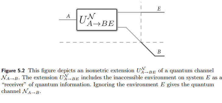
DEfinition 5.2.1 (Isometric Extension) Let $\mathcal{H}A$ and $\mathcal{H}_B$ be Hilbert spaces, and let $\mathcal{N}: \mathcal{L}\left(\mathcal{H}_A\right) \rightarrow \mathcal{L}\left(\mathcal{H}_B\right)$ be a quantum channel. Let $\mathcal{H}_E$ be a Hilbert space with dimension no smaller than the Choi rank of the channel $\mathcal{N}$. An isometric extension or Stinespring dilation $U: \mathcal{H}_A \rightarrow \mathcal{H}_B \otimes \mathcal{H}_E$ of the channel $\mathcal{N}$ is a linear isometry such that $$ \operatorname{Tr}_E\left{U X_A U^{\dagger}\right}=\mathcal{N}{A \rightarrow B}\left(X_A\right),
$$
for $X_A \in \mathcal{L}\left(\mathcal{H}A\right)$. The fact that $U$ is an isometry is equivalent to the following conditions: $$ U^{\dagger} U=I_A, \quad U U^{\dagger}=\Pi{B E},
$$
where $\Pi_{B E}$ is a projection of the tensor-product Hilbert space $\mathcal{H}B \otimes \mathcal{H}_E$. NOtATION 5.2.1 We often write a channel $\mathcal{N}: \mathcal{L}\left(\mathcal{H}_A\right) \rightarrow \mathcal{L}\left(\mathcal{H}_B\right)$ as $\mathcal{N}{A \rightarrow B}$ in order to indicate the input and output systems explicitly. Similarly, we often write an isometric extension $U: \mathcal{H}A \rightarrow \mathcal{H}_B \otimes \mathcal{H}_E$ of $\mathcal{N}$ as $U{A \rightarrow B E}^{\mathcal{N}}$ in order to indicate its association with $\mathcal{N}$ explicitly, as well the fact that it accepts an inputsystem $A$ and has output systems $B$ and $E$. The system $E$ is often referred to as an “environment” system. Finally, there is a quantum channel $\mathcal{U}{A \rightarrow B E}^{\mathcal{N}}$ associated to an isometric extension $U{A \rightarrow B E}^{\mathcal{N}}$, which is defined by
$$
\mathcal{U}{A \rightarrow B E}^{\mathcal{N}}\left(X_A\right)=U X_A U^{\dagger} $$ for $X_A \in \mathcal{L}\left(\mathcal{H}_A\right)$. Note that $\mathcal{U}{A \rightarrow B E}^{\mathcal{N}}$ is a quantum channel with a single Kraus operator $U$ given that $U^{\dagger} U=I_A$.

物理代写|量子力学代写quantum mechanics代考|Isometric Extension from Kraus Operators

It is possible to determine an isometric extension of a quantum channel directly from a set of Kraus operators. Consider a quantum channel $\mathcal{N}{A \rightarrow B}$ with the following Kraus representation: $$ \mathcal{N}{A \rightarrow B}\left(\rho_A\right)=\sum_j N_j \rho_A N_j^{\dagger} .
$$

An isometric extension of the channel $\mathcal{N}{A \rightarrow B}$ is the following linear map: $$ U{A \rightarrow B E}^{\mathcal{N}} \equiv \sum_j N_j \otimes|j\rangle_E .
$$
It is straightforward to verify that the above map is an isometry:
$$
\begin{aligned}
\left(U^{\mathcal{N}}\right)^{\dagger} U^{\mathcal{N}} & =\left(\sum_k N_k^{\dagger} \otimes\left\langle\left. k\right|E\right)\left(\sum_j N_j \otimes|j\rangle_E\right)\right. \ & =\sum{k, j} N_k^{\dagger} N_j\langle k \mid j\rangle \
& =\sum_k N_k^{\dagger} N_k \
& =I_A .
\end{aligned}
$$
The last equality follows from the completeness condition of the Kraus operators. As a consequence, we get that $U^{\mathcal{N}}\left(U^{\mathcal{N}}\right)^{\dagger}$ is a projector on the joint system $B E$, which follows by the same reasoning given in (4.259). Finally, we should verify that $U^{\mathcal{N}}$ is an extension of $\mathcal{N}$. Applying the channel $\mathcal{U}{A \rightarrow B E}^{\mathcal{N}}$ to an arbitrary density operator $\rho_A$ gives the following map: $$ \begin{aligned} \mathcal{U}{A \rightarrow B E}^{\mathcal{N}}\left(\rho_A\right) & \equiv U^{\mathcal{N}} \rho_A\left(U^{\mathcal{N}}\right)^{\dagger} \
& =\left(\sum_j N_j \otimes|j\rangle_E\right) \rho_A\left(\sum_k N_k^{\dagger} \otimes\left\langle\left. k\right|E\right)\right. \ & =\sum{j, k} N_j \rho_A N_k^{\dagger} \otimes|j\rangle\left\langle\left. k\right|E,\right. \end{aligned} $$ and tracing out the environment system gives back the original quantum channel $\mathcal{N}{A \rightarrow B}$ :
$$
\operatorname{Tr}E\left{\mathcal{U}{A \rightarrow B E}^{\mathcal{N}}\left(\rho_A\right)\right}=\sum_j N_j \rho_A N_j^{\dagger}=\mathcal{N}_{A \rightarrow B}\left(\rho_A\right)
$$

物理代写|量子力学代写quantum mechanics代考|Isometric Extension of a Quantum Channel

量子力学代考

物理代写|量子力学代写quantum mechanics代考|Isometric Extension of a Quantum Channel

我们现在给出量子通道等距扩展的一般定义:
定义5.2.1(等距扩展)设$\mathcal{H}A$和$\mathcal{H}B$为希尔伯特空间,设$\mathcal{N}: \mathcal{L}\left(\mathcal{H}_A\right) \rightarrow \mathcal{L}\left(\mathcal{H}_B\right)$为量子通道。设$\mathcal{H}_E$为希尔伯特空间,其维数不小于通道$\mathcal{N}$的Choi秩。通道的等距延伸或弹簧膨胀$U: \mathcal{H}_A \rightarrow \mathcal{H}_B \otimes \mathcal{H}_E$$\mathcal{N}$是线性等距,这样$$ \operatorname{Tr}_E\left{U X_A U^{\dagger}\right}=\mathcal{N}{A \rightarrow B}\left(X_A\right), $$ 浏览$X_A \in \mathcal{L}\left(\mathcal{H}A\right)$。$U$是等距的事实等价于以下条件:$$ U^{\dagger} U=I_A, \quad U U^{\dagger}=\Pi{B E}, $$ 其中$\Pi{B E}$是张量积希尔伯特空间$\mathcal{H}B \otimes \mathcal{H}_E$的投影。5.2.1为了明确地指出输入和输出系统,我们经常将通道$\mathcal{N}: \mathcal{L}\left(\mathcal{H}_A\right) \rightarrow \mathcal{L}\left(\mathcal{H}_B\right)$写成$\mathcal{N}{A \rightarrow B}$。类似地,我们经常将$\mathcal{N}$的等长扩展$U: \mathcal{H}A \rightarrow \mathcal{H}_B \otimes \mathcal{H}_E$写成$U{A \rightarrow B E}^{\mathcal{N}}$,以便显式地表明它与$\mathcal{N}$的关联,以及它接受输入系统$A$并具有输出系统$B$和$E$的事实。系统$E$通常被称为“环境”系统。最后,还有一个与等距扩展$U{A \rightarrow B E}^{\mathcal{N}}$相关联的量子通道$\mathcal{U}{A \rightarrow B E}^{\mathcal{N}}$,它由
$$
\mathcal{U}{A \rightarrow B E}^{\mathcal{N}}\left(X_A\right)=U X_A U^{\dagger} $$代表$X_A \in \mathcal{L}\left(\mathcal{H}_A\right)$。请注意,$\mathcal{U}{A \rightarrow B E}^{\mathcal{N}}$是一个量子信道,具有单个克劳斯算符$U$,假设$U^{\dagger} U=I_A$。

物理代写|量子力学代写quantum mechanics代考|Isometric Extension from Kraus Operators

直接从一组克劳斯算符确定量子信道的等距扩展是可能的。考虑以下克劳斯表示的量子通道$\mathcal{N}{A \rightarrow B}$: $$ \mathcal{N}{A \rightarrow B}\left(\rho_A\right)=\sum_j N_j \rho_A N_j^{\dagger} .
$$

通道$\mathcal{N}{A \rightarrow B}$的等距扩展是以下线性映射:$$ U{A \rightarrow B E}^{\mathcal{N}} \equiv \sum_j N_j \otimes|j\rangle_E .
$$
很容易验证上面的图是等距图:
$$
\begin{aligned}
\left(U^{\mathcal{N}}\right)^{\dagger} U^{\mathcal{N}} & =\left(\sum_k N_k^{\dagger} \otimes\left\langle\left. k\right|E\right)\left(\sum_j N_j \otimes|j\rangle_E\right)\right. \ & =\sum{k, j} N_k^{\dagger} N_j\langle k \mid j\rangle \
& =\sum_k N_k^{\dagger} N_k \
& =I_A .
\end{aligned}
$$
最后一个等式由Kraus算子的完备性条件推导出来。因此,我们得到$U^{\mathcal{N}}\left(U^{\mathcal{N}}\right)^{\dagger}$是关节系统$B E$上的投影仪,这与(4.259)中给出的推理相同。最后,我们应该验证$U^{\mathcal{N}}$是$\mathcal{N}$的扩展。将信道$\mathcal{U}{A \rightarrow B E}^{\mathcal{N}}$应用于任意密度算子$\rho_A$,得到以下映射:$$ \begin{aligned} \mathcal{U}{A \rightarrow B E}^{\mathcal{N}}\left(\rho_A\right) & \equiv U^{\mathcal{N}} \rho_A\left(U^{\mathcal{N}}\right)^{\dagger} \
& =\left(\sum_j N_j \otimes|j\rangle_E\right) \rho_A\left(\sum_k N_k^{\dagger} \otimes\left\langle\left. k\right|E\right)\right. \ & =\sum{j, k} N_j \rho_A N_k^{\dagger} \otimes|j\rangle\left\langle\left. k\right|E,\right. \end{aligned} $$并跟踪环境系统,返回原始量子信道$\mathcal{N}{A \rightarrow B}$:
$$
\operatorname{Tr}E\left{\mathcal{U}{A \rightarrow B E}^{\mathcal{N}}\left(\rho_A\right)\right}=\sum_j N_j \rho_A N_j^{\dagger}=\mathcal{N}_{A \rightarrow B}\left(\rho_A\right)
$$

物理代写|量子力学代写quantum mechanics代考 请认准statistics-lab™

统计代写请认准statistics-lab™. statistics-lab™为您的留学生涯保驾护航。

R语言代写问卷设计与分析代写
PYTHON代写回归分析与线性模型代写
MATLAB代写方差分析与试验设计代写
STATA代写机器学习/统计学习代写
SPSS代写计量经济学代写
EVIEWS代写时间序列分析代写
EXCEL代写深度学习代写
SQL代写各种数据建模与可视化代写

物理代写|量子力学代写quantum mechanics代考|Erasure Channels

如果你也在 怎样代写量子力学Quantum mechanics这个学科遇到相关的难题,请随时右上角联系我们的24/7代写客服。量子力学Quantum mechanics在理论物理学中,量子场论(QFT)是一个结合了经典场论、狭义相对论和量子力学的理论框架。QFT在粒子物理学中用于构建亚原子粒子的物理模型,在凝聚态物理学中用于构建准粒子的模型。

量子力学Quantum mechanics产生于跨越20世纪大部分时间的几代理论物理学家的工作。它的发展始于20世纪20年代对光和电子之间相互作用的描述,最终形成了第一个量子场理论–量子电动力学。随着微扰计算中各种无限性的出现和持续存在,一个主要的理论障碍很快出现了,这个问题直到20世纪50年代随着重正化程序的发明才得以解决。第二个主要障碍是QFT显然无法描述弱相互作用和强相互作用,以至于一些理论家呼吁放弃场论方法。20世纪70年代,规整理论的发展和标准模型的完成导致了量子场论的复兴。

statistics-lab™ 为您的留学生涯保驾护航 在代写量子力学quantum mechanics方面已经树立了自己的口碑, 保证靠谱, 高质且原创的统计Statistics代写服务。我们的专家在代写量子力学quantum mechanics代写方面经验极为丰富,各种代写量子力学quantum mechanics相关的作业也就用不着说。

物理代写|量子力学代写quantum mechanics代考|Erasure Channels

物理代写|量子力学代写quantum mechanics代考|Erasure Channels

The erasure channel is another important channel in quantum Shannon theory. It admits a simple model and is amenable to relatively straightforward analysis when we later discuss its capacity. The erasure channel can serve as a simplified model of photon loss in optical systems.

We first recall the classical definition of an erasure channel. A classical erasure channel either transmits a bit with some probability $1-\varepsilon$ or replaces it with an erasure symbol $e$ with some probability $\varepsilon$. The output alphabet contains one more symbol than the input alphabet, namely, the erasure symbol $e$.

The generalization of the classical erasure channel to the quantum world is straightforward. It implements the following map:
$$
\rho \rightarrow(1-\varepsilon) \rho+\varepsilon|e\rangle\langle e|,
$$
where $|e\rangle$ is some state that is not in the input Hilbert space, and thus is orthogonal to it. The output space of the erasure channel is larger than its input space by one dimension. The interpretation of the quantum erasure channel is similar to that for the classical erasure channel. It transmits a qubit with probability $1-\varepsilon$ and “erases” it (replaces it with an orthogonal erasure state) with probability $\varepsilon$.

物理代写|量子力学代写quantum mechanics代考|Conditional Quantum Channels

We end this chapter by considering one final type of evolution. A conditional quantum encoder $\mathcal{E}{M A \rightarrow B}$, or conditional quantum channel, is a collection $\left{\mathcal{E}{A \rightarrow B}^m\right}_m$ of CPTP maps. Its inputs are a classical system $M$ and a quantum system $A$ and its output is a quantum system $B$. A conditional quantum encoder can function as an encoder of both classical and quantum information.
A classical-quantum state $\rho_{M A}$, where
$$
\rho_{M A} \equiv \sum_m p(m)|m\rangle\left\langle\left. m\right|M \otimes \rho_A^m,\right. $$ can act as an input to a conditional quantum encoder $\mathcal{E}{M A \rightarrow B}$. The action of the conditional quantum encoder $\mathcal{E}{M A \rightarrow B}$ on the classical-quantum state $\rho{M A}$ is as follows:
$$
\mathcal{E}{M A \rightarrow B}\left(\rho{M A}\right)=\operatorname{Tr}M\left{\sum_m p(m)|m\rangle\left\langle\left. m\right|_M \otimes \mathcal{E}{A \rightarrow B}^m\left(\rho_A^m\right)\right} .\right.
$$
Figure 4.5 depicts the behavior of the conditional quantum encoder.
It is actually possible to write any quantum channel as a conditional quantum encoder when its input is a classical-quantum state. Indeed, consider any quantum channel $\mathcal{N}_{X A \rightarrow B}$ that has input systems $X$ and $A$ and output system $B$.

物理代写|量子力学代写quantum mechanics代考|Erasure Channels

量子力学代考

物理代写|量子力学代写quantum mechanics代考|Erasure Channels

擦除信道是量子香农理论中的另一个重要信道。它允许一个简单的模型,并且在我们稍后讨论它的能力时,可以进行相对直接的分析。在光学系统中,擦除通道可以作为光子损耗的简化模型。

我们首先回顾一下擦除通道的经典定义。经典的擦除信道要么以某种概率$1-\varepsilon$传输位,要么以某种概率$\varepsilon$将其替换为擦除符号$e$。输出字母比输入字母多包含一个符号,即擦除符号$e$。

将经典的擦除信道推广到量子世界是很简单的。它实现了以下映射:
$$
\rho \rightarrow(1-\varepsilon) \rho+\varepsilon|e\rangle\langle e|,
$$
其中$|e\rangle$是某个不在输入希尔伯特空间中的状态,因此与它正交。擦除通道的输出空间比其输入空间大一个维度。量子擦除信道的解释与经典擦除信道的解释相似。它以$1-\varepsilon$的概率传输量子比特,并以$\varepsilon$的概率“擦除”它(用正交擦除状态替换它)。

物理代写|量子力学代写quantum mechanics代考|Conditional Quantum Channels

我们以最后一种进化形式来结束本章。条件量子编码器$\mathcal{E}{M A \rightarrow B}$,或条件量子信道,是一个集合$\left{\mathcal{E}{A \rightarrow B}^m\right}m$的CPTP映射。它的输入是经典系统$M$和量子系统$A$它的输出是量子系统$B$。条件量子编码器可以同时作为经典信息和量子信息的编码器。 经典量子态$\rho{M A}$,其中
$$
\rho_{M A} \equiv \sum_m p(m)|m\rangle\left\langle\left. m\right|M \otimes \rho_A^m,\right. $$可以作为条件量子编码器$\mathcal{E}{M A \rightarrow B}$的输入。条件量子编码器$\mathcal{E}{M A \rightarrow B}$对经典量子态$\rho{M A}$的作用如下:
$$
\mathcal{E}{M A \rightarrow B}\left(\rho{M A}\right)=\operatorname{Tr}M\left{\sum_m p(m)|m\rangle\left\langle\left. m\right|M \otimes \mathcal{E}{A \rightarrow B}^m\left(\rho_A^m\right)\right} .\right. $$ 图4.5描述了条件量子编码器的行为。 当量子信道的输入是经典量子态时,实际上可以将其写入条件量子编码器。实际上,考虑任何具有输入系统$X$和$A$以及输出系统$B$的量子通道$\mathcal{N}{X A \rightarrow B}$。

物理代写|量子力学代写quantum mechanics代考 请认准statistics-lab™

统计代写请认准statistics-lab™. statistics-lab™为您的留学生涯保驾护航。

R语言代写问卷设计与分析代写
PYTHON代写回归分析与线性模型代写
MATLAB代写方差分析与试验设计代写
STATA代写机器学习/统计学习代写
SPSS代写计量经济学代写
EVIEWS代写时间序列分析代写
EXCEL代写深度学习代写
SQL代写各种数据建模与可视化代写

物理代写|量子力学代写quantum mechanics代考|Classical-to-Classical Channels

如果你也在 怎样代写量子力学Quantum mechanics这个学科遇到相关的难题,请随时右上角联系我们的24/7代写客服。量子力学Quantum mechanics在理论物理学中,量子场论(QFT)是一个结合了经典场论、狭义相对论和量子力学的理论框架。QFT在粒子物理学中用于构建亚原子粒子的物理模型,在凝聚态物理学中用于构建准粒子的模型。

量子力学Quantum mechanics产生于跨越20世纪大部分时间的几代理论物理学家的工作。它的发展始于20世纪20年代对光和电子之间相互作用的描述,最终形成了第一个量子场理论–量子电动力学。随着微扰计算中各种无限性的出现和持续存在,一个主要的理论障碍很快出现了,这个问题直到20世纪50年代随着重正化程序的发明才得以解决。第二个主要障碍是QFT显然无法描述弱相互作用和强相互作用,以至于一些理论家呼吁放弃场论方法。20世纪70年代,规整理论的发展和标准模型的完成导致了量子场论的复兴。

statistics-lab™ 为您的留学生涯保驾护航 在代写量子力学quantum mechanics方面已经树立了自己的口碑, 保证靠谱, 高质且原创的统计Statistics代写服务。我们的专家在代写量子力学quantum mechanics代写方面经验极为丰富,各种代写量子力学quantum mechanics相关的作业也就用不着说。

物理代写|量子力学代写quantum mechanics代考|Classical-to-Classical Channels

物理代写|量子力学代写quantum mechanics代考|Classical-to-Classical Channels

It is natural to expect that classical channels are special cases of quantum channels, and indeed, this is the case. To see this, fix an input probability distribution $p_X(x)$ and a classical channel $p_{Y \mid X}(y \mid x)$. Fix an orthonormal basis ${|x\rangle}$ corresponding to the input letters and an orthonormal basis ${|y\rangle}$ corresponding to the output letters. We can then encode the input probability distribution $p_X(x)$ as a density operator $\rho$ of the following form:
$$
\rho=\sum_x p_X(x)|x\rangle\langle x|
$$
Let $\mathcal{N}$ be a quantum channel with the following Kraus operators
$$
\left{\sqrt{p_{Y \mid X}(y \mid x)}|y\rangle\langle x|\right}_{x, y} .
$$
(The fact that these are legitimate Kraus operators follows directly from the fact that $p_{Y \mid X}(y \mid x)$ is a conditional probability distribution.) The quantum channel then has the following action on the input $\rho$ :
$$
\begin{aligned}
\mathcal{N}(\rho) & =\sum_{x, y} \sqrt{p_{Y \mid X}(y \mid x)}|y\rangle\left\langle x\left|\left(\sum_{x^{\prime}} p_X\left(x^{\prime}\right)\left|x^{\prime}\right\rangle\left\langle x^{\prime}\right|\right) \sqrt{p_{Y \mid X}(y \mid x)}\right| x\right\rangle\langle y| \
& =\sum_{x, y, x^{\prime}} p_{Y \mid X}(y \mid x) p_X\left(x^{\prime}\right)\left|\left\langle x^{\prime} \mid x\right\rangle\right|^2|y\rangle\langle y| \
& =\sum_{x, y} p_{Y \mid X}(y \mid x) p_X(x)|y\rangle\langle y| \
& =\sum_y\left(\sum_x p_{Y \mid X}(y \mid x) p_X(x)\right)|y\rangle\langle y| .
\end{aligned}
$$

物理代写|量子力学代写quantum mechanics代考|Classical-to-Quantum Channels

Classical-to-quantum channels, or classical-quantum channels for short, are channels which take classical systems to quantum systems. They thus go one step beyond both classical-to-classical channels and preparation channels. More generally, they make a given quantum system classical and then prepare a quantum state, as discussed in the following definition:

DEFInition 4.6.6 (Classical-Quantum Channel) A classical-quantum channel first measures the input state in a particular orthonormal basis and outputs a density operator conditioned on the result of the measurement. Given an orthonormal basis $\left{|k\rangle_A\right}$ and a set of states $\left{\sigma_B^k\right}$, each of which is in $\mathcal{D}\left(\mathcal{H}_B\right)$, a classical-quantum channel has the following action on an input density operator $\rho_A \in \mathcal{D}\left(\mathcal{H}_A\right):$
$$
\rho_A \rightarrow \sum_k\left\langle\left. k\right|_A \rho_A \mid k\right\rangle_A \sigma_B^k .
$$
Let us see how this comes about, using the definition above. The classicalquantum channel first measures the input state $\rho_A$ in the basis $\left{|k\rangle_A\right}$. Given that the result of the measurement is $k$, the post measurement state is
$$
\frac{|k\rangle\left\langle k\left|\rho_A\right| k\right\rangle\langle k|}{\left\langle k\left|\rho_A\right| k\right\rangle} .
$$
The channel then correlates a density operator $\sigma_B^k$ with the post-measurement state $k$ :
$$
\frac{|k\rangle\left\langle k\left|\rho_A\right| k\right\rangle\langle k|}{\left\langle k\left|\rho_A\right| k\right\rangle} \otimes \sigma_B^k .
$$

物理代写|量子力学代写quantum mechanics代考|Classical-to-Classical Channels

量子力学代考

物理代写|量子力学代写quantum mechanics代考|Classical-to-Classical Channels

我们很自然地认为经典通道是量子通道的特殊情况,事实也确实如此。要看到这一点,固定一个输入概率分布$p_X(x)$和一个经典通道$p_{Y \mid X}(y \mid x)$。固定输入字母对应的标准正交基${|x\rangle}$和输出字母对应的标准正交基${|y\rangle}$。然后我们可以将输入概率分布$p_X(x)$编码为如下形式的密度算子$\rho$:
$$
\rho=\sum_x p_X(x)|x\rangle\langle x|
$$
设$\mathcal{N}$为具有以下克劳斯算符的量子信道
$$
\left{\sqrt{p_{Y \mid X}(y \mid x)}|y\rangle\langle x|\right}{x, y} . $$ (这些都是合法的Kraus运算符,这一事实直接源于$p{Y \mid X}(y \mid x)$是一个条件概率分布。)然后量子通道对输入$\rho$有以下动作:
$$
\begin{aligned}
\mathcal{N}(\rho) & =\sum_{x, y} \sqrt{p_{Y \mid X}(y \mid x)}|y\rangle\left\langle x\left|\left(\sum_{x^{\prime}} p_X\left(x^{\prime}\right)\left|x^{\prime}\right\rangle\left\langle x^{\prime}\right|\right) \sqrt{p_{Y \mid X}(y \mid x)}\right| x\right\rangle\langle y| \
& =\sum_{x, y, x^{\prime}} p_{Y \mid X}(y \mid x) p_X\left(x^{\prime}\right)\left|\left\langle x^{\prime} \mid x\right\rangle\right|^2|y\rangle\langle y| \
& =\sum_{x, y} p_{Y \mid X}(y \mid x) p_X(x)|y\rangle\langle y| \
& =\sum_y\left(\sum_x p_{Y \mid X}(y \mid x) p_X(x)\right)|y\rangle\langle y| .
\end{aligned}
$$

物理代写|量子力学代写quantum mechanics代考|Classical-to-Quantum Channels

经典到量子通道,或简称经典量子通道,是将经典系统传输到量子系统的通道。因此,他们超越了古典到古典的渠道和准备渠道。更一般地说,它们使给定的量子系统变得经典,然后制备量子态,如下面的定义所述:

定义4.6.6(经典量子通道)经典量子通道首先以特定的标准正交基测量输入状态,并根据测量结果输出密度算子。给定一个标准正交基$\left{|k\rangle_A\right}$和一组状态$\left{\sigma_B^k\right}$,其中每个都在$\mathcal{D}\left(\mathcal{H}_B\right)$中,经典量子通道对输入密度算子$\rho_A \in \mathcal{D}\left(\mathcal{H}_A\right):$具有以下作用
$$
\rho_A \rightarrow \sum_k\left\langle\left. k\right|_A \rho_A \mid k\right\rangle_A \sigma_B^k .
$$
让我们用上面的定义来看看这是怎么发生的。经典量子通道首先测量基$\left{|k\rangle_A\right}$中的输入状态$\rho_A$。假设测量结果为$k$,则测量后的状态为
$$
\frac{|k\rangle\left\langle k\left|\rho_A\right| k\right\rangle\langle k|}{\left\langle k\left|\rho_A\right| k\right\rangle} .
$$
然后通道将密度算子$\sigma_B^k$与测量后状态$k$关联起来:
$$
\frac{|k\rangle\left\langle k\left|\rho_A\right| k\right\rangle\langle k|}{\left\langle k\left|\rho_A\right| k\right\rangle} \otimes \sigma_B^k .
$$

物理代写|量子力学代写quantum mechanics代考 请认准statistics-lab™

统计代写请认准statistics-lab™. statistics-lab™为您的留学生涯保驾护航。

R语言代写问卷设计与分析代写
PYTHON代写回归分析与线性模型代写
MATLAB代写方差分析与试验设计代写
STATA代写机器学习/统计学习代写
SPSS代写计量经济学代写
EVIEWS代写时间序列分析代写
EXCEL代写深度学习代写
SQL代写各种数据建模与可视化代写

物理代写|量子力学代写quantum mechanics代考|Serial Concatenation of Quantum Channels

如果你也在 怎样代写量子力学Quantum mechanics这个学科遇到相关的难题,请随时右上角联系我们的24/7代写客服。量子力学Quantum mechanics在理论物理学中,量子场论(QFT)是一个结合了经典场论、狭义相对论和量子力学的理论框架。QFT在粒子物理学中用于构建亚原子粒子的物理模型,在凝聚态物理学中用于构建准粒子的模型。

量子力学Quantum mechanics产生于跨越20世纪大部分时间的几代理论物理学家的工作。它的发展始于20世纪20年代对光和电子之间相互作用的描述,最终形成了第一个量子场理论–量子电动力学。随着微扰计算中各种无限性的出现和持续存在,一个主要的理论障碍很快出现了,这个问题直到20世纪50年代随着重正化程序的发明才得以解决。第二个主要障碍是QFT显然无法描述弱相互作用和强相互作用,以至于一些理论家呼吁放弃场论方法。20世纪70年代,规整理论的发展和标准模型的完成导致了量子场论的复兴。

statistics-lab™ 为您的留学生涯保驾护航 在代写量子力学quantum mechanics方面已经树立了自己的口碑, 保证靠谱, 高质且原创的统计Statistics代写服务。我们的专家在代写量子力学quantum mechanics代写方面经验极为丰富,各种代写量子力学quantum mechanics相关的作业也就用不着说。

物理代写|量子力学代写quantum mechanics代考|Serial Concatenation of Quantum Channels

物理代写|量子力学代写quantum mechanics代考|Serial Concatenation of Quantum Channels

A quantum state may undergo not just one type of quantum evolution-it can of course undergo one quantum channel followed by another quantum channel. Let $\mathcal{N}: \mathcal{L}\left(\mathcal{H}A\right) \rightarrow \mathcal{L}\left(\mathcal{H}_B\right)$ denote a first quantum channel and let $\mathcal{M}: \mathcal{L}\left(\mathcal{H}_B\right) \rightarrow$ $\mathcal{L}\left(\mathcal{H}_C\right)$ denote a second quantum channel. Suppose that the Kraus operators of $\mathcal{N}$ are $\left{N_k\right}$ and the Kraus operators of $\mathcal{M}$ are $\left{M_k\right}$. It is straightforward to define the serial concatenation $\mathcal{M}{B \rightarrow C} \circ \mathcal{N}{A \rightarrow B}$ of these two quantum channels. Consider that the output of the first channel is $$ \mathcal{N}{A \rightarrow B}\left(\rho_A\right) \equiv \sum_k N_k \rho_A N_k^{\dagger}
$$
for some input density operator $\rho_A \in \mathcal{D}\left(\mathcal{H}A\right)$. The output of the serially concatenated channel $\mathcal{M}{B \rightarrow C} \circ \mathcal{N}{A \rightarrow B}$ is then $$ \left(\mathcal{M}{B \rightarrow C} \circ \mathcal{N}{A \rightarrow B}\right)\left(\rho_A\right)=\sum_k M_k \mathcal{N}{A \rightarrow B}(\rho) M_k^{\dagger}=\sum_{k, k^{\prime}} M_k N_{k^{\prime}} \rho_A N_{k^{\prime}}^{\dagger} M_k^{\dagger}
$$
It is clear that the Kraus operators of the serially concatenated channel $\mathcal{M}{B \rightarrow C} \circ \mathcal{N}{A \rightarrow B}$ are $\left{M_k N_{k^{\prime}}\right}_{k, k^{\prime}}$. Serial concatenation of channels has an obvious generalization to a serial concatenation of more than two channels.

物理代写|量子力学代写quantum mechanics代考|Parallel Concatenation of Quantum Channels

We can also use two channels in parallel. That is, suppose that we send a system $A$ through a channel $\mathcal{N}: \mathcal{L}\left(\mathcal{H}A\right) \rightarrow \mathcal{L}\left(\mathcal{H}_C\right)$ and a system $B$ through a channel $\mathcal{M}: \mathcal{L}\left(\mathcal{H}_B\right) \rightarrow \mathcal{L}\left(\mathcal{H}_D\right)$. Suppose further that the Kraus operators of $\mathcal{N}{A \rightarrow C}$ are $\left{N_k\right}$ and those for $\mathcal{M}{B \rightarrow D}$ are $\left{M{k^{\prime}}\right}$. Then the parallel concatenation of the two channels is equal to the following serial concatenation:
$$
\mathcal{N}{A \rightarrow C} \otimes \mathcal{M}{B \rightarrow D}=\left(\mathcal{N}{A \rightarrow C} \otimes \mathrm{id}_D\right)\left(\mathrm{id}_A \otimes \mathcal{M}{B \rightarrow D}\right),
$$
or equivalently
$$
\mathcal{N}{A \rightarrow C} \otimes \mathcal{M}{B \rightarrow D}=\left(\mathrm{id}C \otimes \mathcal{M}{B \rightarrow D}\right)\left(\mathcal{N}{A \rightarrow C} \otimes \mathrm{id}_B\right) $$ Intuitively, if Alice is conducting a local action and Bob is as well, the order in which they conduct their actions does not matter for determining the final output state. We have already discussed that a set of Kraus operators for $\mathcal{N}{A \rightarrow C} \otimes \mathrm{id}_D$ is $\left{N_k \otimes I_D\right}$ and a set for id ${ }A \otimes \mathcal{M}{B \rightarrow D}$ is $\left{I_A \otimes M_{k^{\prime}}\right}$, so that it is straightforward to verify that a set of Kraus operators for $\mathcal{N}{A \rightarrow C} \otimes \mathcal{M}{B \rightarrow D}$ is $\left{N_k \otimes M_{k^{\prime}}\right}$. The parallel concatenated channel $\mathcal{N}{A \rightarrow C} \otimes \mathcal{M}{B \rightarrow D}$ thus has the following action on an input density operator $\rho_{A B} \in \mathcal{D}\left(\mathcal{H}A \otimes \mathcal{H}_B\right)$ : $$ \left(\mathcal{N}{A \rightarrow C} \otimes \mathcal{M}{B \rightarrow D}\right)\left(\rho{A B}\right)=\sum_{k, k^{\prime}}\left(N_k \otimes M_{k^{\prime}}\right)\left(\rho_{A B}\right)\left(N_k \otimes M_{k^{\prime}}\right)^{\dagger}
$$
Parallel concatenation of channels also has an obvious generalization to more than two channels.

物理代写|量子力学代写quantum mechanics代考|Serial Concatenation of Quantum Channels

量子力学代考

物理代写|量子力学代写quantum mechanics代考|Serial Concatenation of Quantum Channels

一个量子态可能不仅仅经历一种类型的量子演化——它当然可以经历一个量子通道接着另一个量子通道。设$\mathcal{N}: \mathcal{L}\left(\mathcal{H}A\right) \rightarrow \mathcal{L}\left(\mathcal{H}B\right)$表示第一量子信道,设$\mathcal{M}: \mathcal{L}\left(\mathcal{H}_B\right) \rightarrow$$\mathcal{L}\left(\mathcal{H}_C\right)$表示第二量子信道。假设$\mathcal{N}$的Kraus算子为$\left{N_k\right}$, $\mathcal{M}$的Kraus算子为$\left{M_k\right}$。定义这两个量子通道的串行连接$\mathcal{M}{B \rightarrow C} \circ \mathcal{N}{A \rightarrow B}$是很简单的。假设第一个通道的输出是$$ \mathcal{N}{A \rightarrow B}\left(\rho_A\right) \equiv \sum_k N_k \rho_A N_k^{\dagger} $$ 对于某个输入密度算子$\rho_A \in \mathcal{D}\left(\mathcal{H}A\right)$。然后,串行连接通道$\mathcal{M}{B \rightarrow C} \circ \mathcal{N}{A \rightarrow B}$的输出为$$ \left(\mathcal{M}{B \rightarrow C} \circ \mathcal{N}{A \rightarrow B}\right)\left(\rho_A\right)=\sum_k M_k \mathcal{N}{A \rightarrow B}(\rho) M_k^{\dagger}=\sum{k, k^{\prime}} M_k N_{k^{\prime}} \rho_A N_{k^{\prime}}^{\dagger} M_k^{\dagger}
$$
很明显,串行连接通道$\mathcal{M}{B \rightarrow C} \circ \mathcal{N}{A \rightarrow B}$的克劳斯操作符是$\left{M_k N_{k^{\prime}}\right}_{k, k^{\prime}}$。信道的串行连接对于两个以上信道的串行连接具有明显的泛化作用。

物理代写|量子力学代写quantum mechanics代考|Parallel Concatenation of Quantum Channels

我们也可以同时使用两个通道。也就是说,假设我们通过通道$\mathcal{N}: \mathcal{L}\left(\mathcal{H}A\right) \rightarrow \mathcal{L}\left(\mathcal{H}C\right)$发送系统$A$,通过通道$\mathcal{M}: \mathcal{L}\left(\mathcal{H}_B\right) \rightarrow \mathcal{L}\left(\mathcal{H}_D\right)$发送系统$B$。进一步假设$\mathcal{N}{A \rightarrow C}$的Kraus算子是$\left{N_k\right}$, $\mathcal{M}{B \rightarrow D}$的Kraus算子是$\left{M{k^{\prime}}\right}$。那么两个通道的并行连接等于下面的串行连接: $$ \mathcal{N}{A \rightarrow C} \otimes \mathcal{M}{B \rightarrow D}=\left(\mathcal{N}{A \rightarrow C} \otimes \mathrm{id}_D\right)\left(\mathrm{id}_A \otimes \mathcal{M}{B \rightarrow D}\right), $$ 或者等价地 $$ \mathcal{N}{A \rightarrow C} \otimes \mathcal{M}{B \rightarrow D}=\left(\mathrm{id}C \otimes \mathcal{M}{B \rightarrow D}\right)\left(\mathcal{N}{A \rightarrow C} \otimes \mathrm{id}_B\right) $$直观地说,如果Alice在执行一个局部操作,Bob也在执行,那么他们执行操作的顺序对于确定最终输出状态并不重要。我们已经讨论过$\mathcal{N}{A \rightarrow C} \otimes \mathrm{id}_D$的一组Kraus操作符是$\left{N_k \otimes I_D\right}$, id ${ }A \otimes \mathcal{M}{B \rightarrow D}$的一组Kraus操作符是$\left{I_A \otimes M{k^{\prime}}\right}$,因此很容易验证$\mathcal{N}{A \rightarrow C} \otimes \mathcal{M}{B \rightarrow D}$的一组Kraus操作符是$\left{N_k \otimes M_{k^{\prime}}\right}$。因此,并行连接通道$\mathcal{N}{A \rightarrow C} \otimes \mathcal{M}{B \rightarrow D}$对输入密度运算符$\rho_{A B} \in \mathcal{D}\left(\mathcal{H}A \otimes \mathcal{H}B\right)$有以下操作:$$ \left(\mathcal{N}{A \rightarrow C} \otimes \mathcal{M}{B \rightarrow D}\right)\left(\rho{A B}\right)=\sum{k, k^{\prime}}\left(N_k \otimes M_{k^{\prime}}\right)\left(\rho_{A B}\right)\left(N_k \otimes M_{k^{\prime}}\right)^{\dagger}
$$
通道的并行连接也有一个明显的泛化到两个以上的通道。

物理代写|量子力学代写quantum mechanics代考 请认准statistics-lab™

统计代写请认准statistics-lab™. statistics-lab™为您的留学生涯保驾护航。

金融工程代写

金融工程是使用数学技术来解决金融问题。金融工程使用计算机科学、统计学、经济学和应用数学领域的工具和知识来解决当前的金融问题,以及设计新的和创新的金融产品。

非参数统计代写

非参数统计指的是一种统计方法,其中不假设数据来自于由少数参数决定的规定模型;这种模型的例子包括正态分布模型和线性回归模型。

广义线性模型代考

广义线性模型(GLM)归属统计学领域,是一种应用灵活的线性回归模型。该模型允许因变量的偏差分布有除了正态分布之外的其它分布。

术语 广义线性模型(GLM)通常是指给定连续和/或分类预测因素的连续响应变量的常规线性回归模型。它包括多元线性回归,以及方差分析和方差分析(仅含固定效应)。

有限元方法代写

有限元方法(FEM)是一种流行的方法,用于数值解决工程和数学建模中出现的微分方程。典型的问题领域包括结构分析、传热、流体流动、质量运输和电磁势等传统领域。

有限元是一种通用的数值方法,用于解决两个或三个空间变量的偏微分方程(即一些边界值问题)。为了解决一个问题,有限元将一个大系统细分为更小、更简单的部分,称为有限元。这是通过在空间维度上的特定空间离散化来实现的,它是通过构建对象的网格来实现的:用于求解的数值域,它有有限数量的点。边界值问题的有限元方法表述最终导致一个代数方程组。该方法在域上对未知函数进行逼近。[1] 然后将模拟这些有限元的简单方程组合成一个更大的方程系统,以模拟整个问题。然后,有限元通过变化微积分使相关的误差函数最小化来逼近一个解决方案。

tatistics-lab作为专业的留学生服务机构,多年来已为美国、英国、加拿大、澳洲等留学热门地的学生提供专业的学术服务,包括但不限于Essay代写,Assignment代写,Dissertation代写,Report代写,小组作业代写,Proposal代写,Paper代写,Presentation代写,计算机作业代写,论文修改和润色,网课代做,exam代考等等。写作范围涵盖高中,本科,研究生等海外留学全阶段,辐射金融,经济学,会计学,审计学,管理学等全球99%专业科目。写作团队既有专业英语母语作者,也有海外名校硕博留学生,每位写作老师都拥有过硬的语言能力,专业的学科背景和学术写作经验。我们承诺100%原创,100%专业,100%准时,100%满意。

随机分析代写


随机微积分是数学的一个分支,对随机过程进行操作。它允许为随机过程的积分定义一个关于随机过程的一致的积分理论。这个领域是由日本数学家伊藤清在第二次世界大战期间创建并开始的。

时间序列分析代写

随机过程,是依赖于参数的一组随机变量的全体,参数通常是时间。 随机变量是随机现象的数量表现,其时间序列是一组按照时间发生先后顺序进行排列的数据点序列。通常一组时间序列的时间间隔为一恒定值(如1秒,5分钟,12小时,7天,1年),因此时间序列可以作为离散时间数据进行分析处理。研究时间序列数据的意义在于现实中,往往需要研究某个事物其随时间发展变化的规律。这就需要通过研究该事物过去发展的历史记录,以得到其自身发展的规律。

回归分析代写

多元回归分析渐进(Multiple Regression Analysis Asymptotics)属于计量经济学领域,主要是一种数学上的统计分析方法,可以分析复杂情况下各影响因素的数学关系,在自然科学、社会和经济学等多个领域内应用广泛。

MATLAB代写

MATLAB 是一种用于技术计算的高性能语言。它将计算、可视化和编程集成在一个易于使用的环境中,其中问题和解决方案以熟悉的数学符号表示。典型用途包括:数学和计算算法开发建模、仿真和原型制作数据分析、探索和可视化科学和工程图形应用程序开发,包括图形用户界面构建MATLAB 是一个交互式系统,其基本数据元素是一个不需要维度的数组。这使您可以解决许多技术计算问题,尤其是那些具有矩阵和向量公式的问题,而只需用 C 或 Fortran 等标量非交互式语言编写程序所需的时间的一小部分。MATLAB 名称代表矩阵实验室。MATLAB 最初的编写目的是提供对由 LINPACK 和 EISPACK 项目开发的矩阵软件的轻松访问,这两个项目共同代表了矩阵计算软件的最新技术。MATLAB 经过多年的发展,得到了许多用户的投入。在大学环境中,它是数学、工程和科学入门和高级课程的标准教学工具。在工业领域,MATLAB 是高效研究、开发和分析的首选工具。MATLAB 具有一系列称为工具箱的特定于应用程序的解决方案。对于大多数 MATLAB 用户来说非常重要,工具箱允许您学习应用专业技术。工具箱是 MATLAB 函数(M 文件)的综合集合,可扩展 MATLAB 环境以解决特定类别的问题。可用工具箱的领域包括信号处理、控制系统、神经网络、模糊逻辑、小波、仿真等。

R语言代写问卷设计与分析代写
PYTHON代写回归分析与线性模型代写
MATLAB代写方差分析与试验设计代写
STATA代写机器学习/统计学习代写
SPSS代写计量经济学代写
EVIEWS代写时间序列分析代写
EXCEL代写深度学习代写
SQL代写各种数据建模与可视化代写

物理代写|量子力学代写quantum mechanics代考|Local Density Operators and Partial Trace

如果你也在 怎样代写量子力学Quantum mechanics这个学科遇到相关的难题,请随时右上角联系我们的24/7代写客服。量子力学Quantum mechanics在理论物理学中,量子场论(QFT)是一个结合了经典场论、狭义相对论和量子力学的理论框架。QFT在粒子物理学中用于构建亚原子粒子的物理模型,在凝聚态物理学中用于构建准粒子的模型。

量子力学Quantum mechanics产生于跨越20世纪大部分时间的几代理论物理学家的工作。它的发展始于20世纪20年代对光和电子之间相互作用的描述,最终形成了第一个量子场理论–量子电动力学。随着微扰计算中各种无限性的出现和持续存在,一个主要的理论障碍很快出现了,这个问题直到20世纪50年代随着重正化程序的发明才得以解决。第二个主要障碍是QFT显然无法描述弱相互作用和强相互作用,以至于一些理论家呼吁放弃场论方法。20世纪70年代,规整理论的发展和标准模型的完成导致了量子场论的复兴。

statistics-lab™ 为您的留学生涯保驾护航 在代写量子力学quantum mechanics方面已经树立了自己的口碑, 保证靠谱, 高质且原创的统计Statistics代写服务。我们的专家在代写量子力学quantum mechanics代写方面经验极为丰富,各种代写量子力学quantum mechanics相关的作业也就用不着说。

物理代写|量子力学代写quantum mechanics代考|Local Density Operators and Partial Trace

物理代写|量子力学代写quantum mechanics代考|Local Density Operators and Partial Trace

A First Example
Consider the entangled Bell state $\left|\Phi^{+}\right\rangle_{A B}$ shared on systems $A$ and $B$. In the above analyses, we determined a local density operator description for both Alice and Bob. Now, we are curious if it is possible to determine such a local density operator description for Alice and Bob with respect to the state $\left|\Phi^{+}\right\rangle_{A B}$ or more general ones.

As a first approach to this issue, recall that the density operator description arises from its usefulness in determining the probabilities of the outcomes of a particular measurement. We say that the density operator is “the state” of the system because it is a mathematical representation that allows us to compute the probabilities resulting from a physical measurement. So, if we would like to determine a “local density operator,” such a local density operator should predict the result of a local measurement.

Let us consider a local POVM $\left{\Lambda^j\right}_j$ that Alice can perform on her system. The global measurement operators for this local measurement are $\left{\Lambda_A^j \otimes I_B\right}_j$ because nothing (the identity) happens to Bob’s system. The probability of obtaining outcome $j$ when performing this measurement on the state $\left|\Phi^{+}\right\rangle_{A B}$ is
$$
\begin{aligned}
\left\langle\left.\Phi^{+}\right|{A B} \Lambda_A^j \otimes I_B \mid \Phi^{+}\right\rangle{A B} & =\frac{1}{2} \sum_{k, l=0}^1\left\langle\left. k k\right|{A B} \Lambda_A^j \otimes I_B \mid l l\right\rangle{A B} \
& =\frac{1}{2} \sum_{k, l=0}^1\left\langle\left. k\right|_A \Lambda_A^j \mid l\right\rangle_A\langle k \mid l\rangle_B \
& =\frac{1}{2}\left(\left\langle\left. 0\right|_A \Lambda_A^j \mid 0\right\rangle_A+\left\langle\left. 1\right|_A \Lambda_A^j \mid 1\right\rangle_A\right) \
& =\frac{1}{2}\left(\operatorname { T r } \left{\Lambda_A^j|0\rangle\left\langle\left. 0\right|_A\right}+\operatorname{Tr}\left{\Lambda_A^j|1\rangle\left\langle\left. 1\right|_A\right}\right)\right.\right. \
& =\operatorname{Tr}\left{\Lambda_A^j \frac{1}{2}\left(|0\rangle\left\langle\left. 0\right|_A+\mid 1\right\rangle\left\langle\left. 1\right|_A\right)\right}\right. \
& =\operatorname{Tr}\left{\Lambda_A^j \pi_A\right}
\end{aligned}
$$

物理代写|量子力学代写quantum mechanics代考|Partial Trace

In general, we would like to determine a local density operator that predicts the outcomes of all local measurements. The general method for determining a local density operator is to employ the partial trace operation, which we motivate and define here, as a generalization of the example discussed at the beginning of Section 4.3.3.

Suppose that Alice and Bob share a bipartite state $\rho_{A B}$ and that Alice performs a local measurement on her system, described by a POVM $\left{\Lambda_A^j\right}$. Then the overall POVM on the joint system is $\left{\Lambda_A^j \otimes I_B\right}$ because we are assuming that Bob is not doing anything to his system. According to the Born rule, the probability for Alice to receive outcome $j$ after performing the measurement is given by the following expression:
$$
p_J(j)=\operatorname{Tr}\left{\left(\Lambda_A^j \otimes I_B\right) \rho_{A B}\right}
$$
In order to evaluate the trace, we can choose any orthonormal basis that we wish (see Definition 4.1.1 and subsequent statements). Taking $\left{|k\rangle_A\right}$ as an orthonormal basis for Alice’s Hilbert space and $\left{|l\rangle_B\right}$ as an orthonormal basis for Bob’s Hilbert space, the set $\left{|k\rangle_A \otimes|l\rangle_B\right}$ constitutes an orthonormal basis for the tensor product of their Hilbert spaces. So we can evaluate (4.138) as follows:
$$
\begin{aligned}
& \operatorname{Tr}\left{\left(\Lambda_A^j \otimes I_B\right) \rho_{A B}\right} \
& =\sum_{k, l}\left(\left\langle\left.k\right|A \otimes\left\langle\left. l\right|_B\right)\left[\left(\Lambda_A^j \otimes I_B\right) \rho{A B}\right]\left(|k\rangle_A \otimes|l\rangle_B\right)\right.\right.
\end{aligned}
$$

$$
\begin{aligned}
& =\sum_{k, l}\left\langlek | _ { A } \left( I_A \otimes\left\langle\left. l\right|B\right)\left[\left(\Lambda_A^j \otimes I_B\right) \rho{A B}\right]\left(I_A \otimes|l\rangle_B\right)|k\rangle_A\right.\right. \
& =\sum_{k, l}\left\langlek | _ { A } \Lambda _ { A } ^ { j } \left( I_A \otimes\left\langle\left. l\right|B\right) \rho{A B}\left(I_A \otimes|l\rangle_B\right)|k\rangle_A\right.\right. \
& =\sum_k\left\langlek | _ { A } \Lambda _ { A } ^ { j } \left[\sum_l\left(I_A \otimes\left\langle\left. l\right|B\right) \rho{A B}\left(I_A \otimes|l\rangle_B\right)\right]|k\rangle_A .\right.\right.
\end{aligned}
$$
The first equality follows from the definition of the trace in Definition 4.1.1 and using the orthonormal basis $\left{|k\rangle_A \otimes|l\rangle_B\right}$. The second equality follows because
$$
|k\rangle_A \otimes|l\rangle_B=\left(I_A \otimes|l\rangle_B\right)|k\rangle_A
$$
The third equality follows because
$$
\left(I_A \otimes\left\langle\left. l\right|_B\right)\left(\Lambda_A^j \otimes I_B\right)=\Lambda_A^j\left(I_A \otimes\left\langle\left. l\right|_B\right) .\right.\right.
$$

物理代写|量子力学代写quantum mechanics代考|Local Density Operators and Partial Trace

量子力学代考

物理代写|量子力学代写quantum mechanics代考|Local Density Operators and Partial Trace

第一个例子
考虑在系统$A$和$B$上共享的纠缠贝尔状态$\left|\Phi^{+}\right\rangle_{A B}$。在上述分析中,我们确定了Alice和Bob的局部密度算子描述。现在,我们很好奇是否有可能确定Alice和Bob关于$\left|\Phi^{+}\right\rangle_{A B}$或更一般的状态的局部密度算子描述。

作为解决这个问题的第一种方法,回想一下,密度算子描述源于它在确定特定测量结果的概率方面的有用性。我们说密度算符是系统的“状态”,因为它是一种数学表示,允许我们计算由物理测量产生的概率。因此,如果我们想要确定一个“局部密度算子”,这样的局部密度算子应该预测局部测量的结果。

让我们考虑一个本地POVM $\left{\Lambda^j\right}j$, Alice可以在她的系统上执行它。这个局部度量的全局度量操作符是$\left{\Lambda_A^j \otimes I_B\right}_j$,因为Bob的系统没有发生任何变化(恒等)。在状态$\left|\Phi^{+}\right\rangle{A B}$上执行此测量时获得结果$j$的概率为
$$
\begin{aligned}
\left\langle\left.\Phi^{+}\right|{A B} \Lambda_A^j \otimes I_B \mid \Phi^{+}\right\rangle{A B} & =\frac{1}{2} \sum_{k, l=0}^1\left\langle\left. k k\right|{A B} \Lambda_A^j \otimes I_B \mid l l\right\rangle{A B} \
& =\frac{1}{2} \sum_{k, l=0}^1\left\langle\left. k\right|_A \Lambda_A^j \mid l\right\rangle_A\langle k \mid l\rangle_B \
& =\frac{1}{2}\left(\left\langle\left. 0\right|_A \Lambda_A^j \mid 0\right\rangle_A+\left\langle\left. 1\right|_A \Lambda_A^j \mid 1\right\rangle_A\right) \
& =\frac{1}{2}\left(\operatorname { T r } \left{\Lambda_A^j|0\rangle\left\langle\left. 0\right|_A\right}+\operatorname{Tr}\left{\Lambda_A^j|1\rangle\left\langle\left. 1\right|_A\right}\right)\right.\right. \
& =\operatorname{Tr}\left{\Lambda_A^j \frac{1}{2}\left(|0\rangle\left\langle\left. 0\right|_A+\mid 1\right\rangle\left\langle\left. 1\right|_A\right)\right}\right. \
& =\operatorname{Tr}\left{\Lambda_A^j \pi_A\right}
\end{aligned}
$$

物理代写|量子力学代写quantum mechanics代考|Partial Trace

一般来说,我们希望确定一个局部密度算子来预测所有局部测量的结果。确定局部密度算符的一般方法是使用部分跟踪运算,我们在这里提出并定义它,作为4.3.3节开头讨论的示例的推广。

假设Alice和Bob共享一个二部状态$\rho_{A B}$,并且Alice在她的系统上执行一个由POVM $\left{\Lambda_A^j\right}$描述的局部测量。那么关节系统上的整体POVM是$\left{\Lambda_A^j \otimes I_B\right}$因为我们假设Bob没有对他的系统做任何事情。根据玻恩规则,执行测量后Alice接收到结果$j$的概率由下式给出:
$$
p_J(j)=\operatorname{Tr}\left{\left(\Lambda_A^j \otimes I_B\right) \rho_{A B}\right}
$$
为了计算跟踪,我们可以选择任何我们希望的标准正交基(参见定义4.1.1和随后的语句)。取$\left{|k\rangle_A\right}$作为Alice的Hilbert空间的标准正交基,$\left{|l\rangle_B\right}$作为Bob的Hilbert空间的标准正交基,集合$\left{|k\rangle_A \otimes|l\rangle_B\right}$构成了它们的Hilbert空间的张量积的标准正交基。因此我们可以对式(4.138)求值为:
$$
\begin{aligned}
& \operatorname{Tr}\left{\left(\Lambda_A^j \otimes I_B\right) \rho_{A B}\right} \
& =\sum_{k, l}\left(\left\langle\left.k\right|A \otimes\left\langle\left. l\right|_B\right)\left[\left(\Lambda_A^j \otimes I_B\right) \rho{A B}\right]\left(|k\rangle_A \otimes|l\rangle_B\right)\right.\right.
\end{aligned}
$$

$$
\begin{aligned}
& =\sum_{k, l}\left\langlek | _ { A } \left( I_A \otimes\left\langle\left. l\right|B\right)\left[\left(\Lambda_A^j \otimes I_B\right) \rho{A B}\right]\left(I_A \otimes|l\rangle_B\right)|k\rangle_A\right.\right. \
& =\sum_{k, l}\left\langlek | _ { A } \Lambda _ { A } ^ { j } \left( I_A \otimes\left\langle\left. l\right|B\right) \rho{A B}\left(I_A \otimes|l\rangle_B\right)|k\rangle_A\right.\right. \
& =\sum_k\left\langlek | _ { A } \Lambda _ { A } ^ { j } \left[\sum_l\left(I_A \otimes\left\langle\left. l\right|B\right) \rho{A B}\left(I_A \otimes|l\rangle_B\right)\right]|k\rangle_A .\right.\right.
\end{aligned}
$$
第一个等式来自定义4.1.1中跟踪的定义,并使用标准正交基$\left{|k\rangle_A \otimes|l\rangle_B\right}$。第二个等式是这样的
$$
|k\rangle_A \otimes|l\rangle_B=\left(I_A \otimes|l\rangle_B\right)|k\rangle_A
$$
第三个等式如下,因为
$$
\left(I_A \otimes\left\langle\left. l\right|_B\right)\left(\Lambda_A^j \otimes I_B\right)=\Lambda_A^j\left(I_A \otimes\left\langle\left. l\right|_B\right) .\right.\right.
$$

物理代写|量子力学代写quantum mechanics代考 请认准statistics-lab™

统计代写请认准statistics-lab™. statistics-lab™为您的留学生涯保驾护航。

金融工程代写

金融工程是使用数学技术来解决金融问题。金融工程使用计算机科学、统计学、经济学和应用数学领域的工具和知识来解决当前的金融问题,以及设计新的和创新的金融产品。

非参数统计代写

非参数统计指的是一种统计方法,其中不假设数据来自于由少数参数决定的规定模型;这种模型的例子包括正态分布模型和线性回归模型。

广义线性模型代考

广义线性模型(GLM)归属统计学领域,是一种应用灵活的线性回归模型。该模型允许因变量的偏差分布有除了正态分布之外的其它分布。

术语 广义线性模型(GLM)通常是指给定连续和/或分类预测因素的连续响应变量的常规线性回归模型。它包括多元线性回归,以及方差分析和方差分析(仅含固定效应)。

有限元方法代写

有限元方法(FEM)是一种流行的方法,用于数值解决工程和数学建模中出现的微分方程。典型的问题领域包括结构分析、传热、流体流动、质量运输和电磁势等传统领域。

有限元是一种通用的数值方法,用于解决两个或三个空间变量的偏微分方程(即一些边界值问题)。为了解决一个问题,有限元将一个大系统细分为更小、更简单的部分,称为有限元。这是通过在空间维度上的特定空间离散化来实现的,它是通过构建对象的网格来实现的:用于求解的数值域,它有有限数量的点。边界值问题的有限元方法表述最终导致一个代数方程组。该方法在域上对未知函数进行逼近。[1] 然后将模拟这些有限元的简单方程组合成一个更大的方程系统,以模拟整个问题。然后,有限元通过变化微积分使相关的误差函数最小化来逼近一个解决方案。

tatistics-lab作为专业的留学生服务机构,多年来已为美国、英国、加拿大、澳洲等留学热门地的学生提供专业的学术服务,包括但不限于Essay代写,Assignment代写,Dissertation代写,Report代写,小组作业代写,Proposal代写,Paper代写,Presentation代写,计算机作业代写,论文修改和润色,网课代做,exam代考等等。写作范围涵盖高中,本科,研究生等海外留学全阶段,辐射金融,经济学,会计学,审计学,管理学等全球99%专业科目。写作团队既有专业英语母语作者,也有海外名校硕博留学生,每位写作老师都拥有过硬的语言能力,专业的学科背景和学术写作经验。我们承诺100%原创,100%专业,100%准时,100%满意。

随机分析代写


随机微积分是数学的一个分支,对随机过程进行操作。它允许为随机过程的积分定义一个关于随机过程的一致的积分理论。这个领域是由日本数学家伊藤清在第二次世界大战期间创建并开始的。

时间序列分析代写

随机过程,是依赖于参数的一组随机变量的全体,参数通常是时间。 随机变量是随机现象的数量表现,其时间序列是一组按照时间发生先后顺序进行排列的数据点序列。通常一组时间序列的时间间隔为一恒定值(如1秒,5分钟,12小时,7天,1年),因此时间序列可以作为离散时间数据进行分析处理。研究时间序列数据的意义在于现实中,往往需要研究某个事物其随时间发展变化的规律。这就需要通过研究该事物过去发展的历史记录,以得到其自身发展的规律。

回归分析代写

多元回归分析渐进(Multiple Regression Analysis Asymptotics)属于计量经济学领域,主要是一种数学上的统计分析方法,可以分析复杂情况下各影响因素的数学关系,在自然科学、社会和经济学等多个领域内应用广泛。

MATLAB代写

MATLAB 是一种用于技术计算的高性能语言。它将计算、可视化和编程集成在一个易于使用的环境中,其中问题和解决方案以熟悉的数学符号表示。典型用途包括:数学和计算算法开发建模、仿真和原型制作数据分析、探索和可视化科学和工程图形应用程序开发,包括图形用户界面构建MATLAB 是一个交互式系统,其基本数据元素是一个不需要维度的数组。这使您可以解决许多技术计算问题,尤其是那些具有矩阵和向量公式的问题,而只需用 C 或 Fortran 等标量非交互式语言编写程序所需的时间的一小部分。MATLAB 名称代表矩阵实验室。MATLAB 最初的编写目的是提供对由 LINPACK 和 EISPACK 项目开发的矩阵软件的轻松访问,这两个项目共同代表了矩阵计算软件的最新技术。MATLAB 经过多年的发展,得到了许多用户的投入。在大学环境中,它是数学、工程和科学入门和高级课程的标准教学工具。在工业领域,MATLAB 是高效研究、开发和分析的首选工具。MATLAB 具有一系列称为工具箱的特定于应用程序的解决方案。对于大多数 MATLAB 用户来说非常重要,工具箱允许您学习应用专业技术。工具箱是 MATLAB 函数(M 文件)的综合集合,可扩展 MATLAB 环境以解决特定类别的问题。可用工具箱的领域包括信号处理、控制系统、神经网络、模糊逻辑、小波、仿真等。

R语言代写问卷设计与分析代写
PYTHON代写回归分析与线性模型代写
MATLAB代写方差分析与试验设计代写
STATA代写机器学习/统计学习代写
SPSS代写计量经济学代写
EVIEWS代写时间序列分析代写
EXCEL代写深度学习代写
SQL代写各种数据建模与可视化代写

物理代写|量子力学代写quantum mechanics代考|Noiseless Evolution of an Ensemble

如果你也在 怎样代写量子力学Quantum mechanics这个学科遇到相关的难题,请随时右上角联系我们的24/7代写客服。量子力学Quantum mechanics在理论物理学中,量子场论(QFT)是一个结合了经典场论、狭义相对论和量子力学的理论框架。QFT在粒子物理学中用于构建亚原子粒子的物理模型,在凝聚态物理学中用于构建准粒子的模型。

量子力学Quantum mechanics产生于跨越20世纪大部分时间的几代理论物理学家的工作。它的发展始于20世纪20年代对光和电子之间相互作用的描述,最终形成了第一个量子场理论–量子电动力学。随着微扰计算中各种无限性的出现和持续存在,一个主要的理论障碍很快出现了,这个问题直到20世纪50年代随着重正化程序的发明才得以解决。第二个主要障碍是QFT显然无法描述弱相互作用和强相互作用,以至于一些理论家呼吁放弃场论方法。20世纪70年代,规整理论的发展和标准模型的完成导致了量子场论的复兴。

statistics-lab™ 为您的留学生涯保驾护航 在代写量子力学quantum mechanics方面已经树立了自己的口碑, 保证靠谱, 高质且原创的统计Statistics代写服务。我们的专家在代写量子力学quantum mechanics代写方面经验极为丰富,各种代写量子力学quantum mechanics相关的作业也就用不着说。

物理代写|量子力学代写quantum mechanics代考|Noiseless Evolution of an Ensemble

物理代写|量子力学代写quantum mechanics代考|Noiseless Evolution of an Ensemble

Quantum states can evolve in a noiseless fashion either according to a unitary operator or a measurement. In this section, we determine the noiseless evolution of an ensemble and its corresponding density operator. We also show how density operators evolve under a quantum measurement.

Noiseless Unitary Evolution of a Noisy State
We first consider noiseless evolution according to some unitary $U$. Suppose we have the ensemble $\mathcal{E}$ in (4.2) with density operator $\rho$. Suppose without loss of generality that the state is $\left|\psi_x\right\rangle$. Then the evolution postulate of the noiseless quantum theory gives that the state after the unitary evolution is as follows: $U\left|\psi_x\right\rangle$. This result implies that the evolution leads to a new ensemble
$$
\mathcal{E}U \equiv\left{p_X(x), U\left|\psi_x\right\rangle\right}{x \in \mathcal{X}}
$$
The density operator of the evolved ensemble is
$$
\begin{aligned}
\sum_{x \in \mathcal{X}} p_X(x) U\left|\psi_x\right\rangle\left\langle\psi_x\right| U^{\dagger} & =U\left(\sum_{x \in \mathcal{X}} p_X(x)\left|\psi_x\right\rangle\left\langle\psi_x\right|\right) U^{\dagger} \
& =U \rho U^{\dagger}
\end{aligned}
$$
Thus, the above relation shows that we can keep track of the evolution of the density operator $\rho$, rather than worrying about keeping track of the evolution of every state in the ensemble $\mathcal{E}$. It suffices to keep track of only the density operator evolution because this operator is sufficient to determine probabilities when performing any measurement on the system.

物理代写|量子力学代写quantum mechanics代考|Noiseless Measurement of a Noisy State

In a similar fashion, we can analyze the result of a measurement on a system with ensemble description $\mathcal{E}$ in (4.2). Suppose that we perform a projective measurement with projection operators $\left{\Pi_j\right}_j$ where $\sum_j \Pi_j=I$. The main result of this section is that two things happen after a measurement occurs. First, as shown in the development preceding (4.19), we receive the outcome $j$ with probability $p_J(j)=\operatorname{Tr}\left{\Pi_j \rho\right}$. Second, if the outcome of the measurement is $j$, then the state evolves as follows:
$$
\rho \longrightarrow \frac{\Pi_j \rho \Pi_j}{p_J(j)}
$$
To see the above, let us suppose that the state in the ensemble $\mathcal{E}$ is $\left|\psi_x\right\rangle$. Then the noiseless quantum theory predicts that the probability of obtaining outcome $j$ conditioned on the index $x$ is
$$
p_{J \mid X}(j \mid x)=\left\langle\psi_x\left|\Pi_j\right| \psi_x\right\rangle
$$
and the resulting state is
$$
\frac{\Pi_j\left|\psi_x\right\rangle}{\sqrt{p_{J \mid X}(j \mid x)}}
$$
Supposing that we receive outcome $j$, then we have a new ensemble:
$$
\mathcal{E}j \equiv\left{p{X \mid J}(x \mid j), \frac{\Pi_j\left|\psi_x\right\rangle}{\sqrt{p_{J \mid X}(j \mid x)}}\right}_{x \in \mathcal{X}} .
$$

物理代写|量子力学代写quantum mechanics代考|Noiseless Evolution of an Ensemble

量子力学代考

物理代写|量子力学代写quantum mechanics代考|Noiseless Evolution of an Ensemble

量子态可以根据酉算子或测量以无噪声的方式演化。在本节中,我们确定了一个系综的无噪声演化及其相应的密度算子。我们还展示了密度算符如何在量子测量下演化。

噪声状态的无噪声统一演化
我们首先根据一些酉$U$考虑无噪声进化。假设我们有(4.2)中的集合$\mathcal{E}$和密度算子$\rho$。在不失一般性的前提下,假设状态为$\left|\psi_x\right\rangle$。然后根据无噪声量子理论的演化假设,给出了幺正演化后的状态:$U\left|\psi_x\right\rangle$。这一结果表明演化导致了一个新的系综
$$
\mathcal{E}U \equiv\left{p_X(x), U\left|\psi_x\right\rangle\right}{x \in \mathcal{X}}
$$
演化系综的密度算符为
$$
\begin{aligned}
\sum_{x \in \mathcal{X}} p_X(x) U\left|\psi_x\right\rangle\left\langle\psi_x\right| U^{\dagger} & =U\left(\sum_{x \in \mathcal{X}} p_X(x)\left|\psi_x\right\rangle\left\langle\psi_x\right|\right) U^{\dagger} \
& =U \rho U^{\dagger}
\end{aligned}
$$
因此,上述关系表明,我们可以跟踪密度算子$\rho$的演化,而不必担心跟踪集合中每个状态的演化$\mathcal{E}$。只跟踪密度算子的演化就足够了,因为在对系统执行任何测量时,这个算子足以确定概率。

物理代写|量子力学代写quantum mechanics代考|Noiseless Measurement of a Noisy State

以类似的方式,我们可以用(4.2)中的集成描述$\mathcal{E}$来分析系统上的测量结果。假设我们使用投影算子$\left{\Pi_j\right}j$执行投影测量,其中$\sum_j \Pi_j=I$。本节的主要结果是在测量发生后会发生两件事。首先,如前面(4.19)的开发所示,我们以$p_J(j)=\operatorname{Tr}\left{\Pi_j \rho\right}$的概率得到结果$j$。第二,如果测量的结果是$j$,那么状态演变如下: $$ \rho \longrightarrow \frac{\Pi_j \rho \Pi_j}{p_J(j)} $$ 要查看上面的内容,让我们假设集合$\mathcal{E}$中的状态为$\left|\psi_x\right\rangle$。然后利用无噪声量子理论预测,以指标$x$为条件的得到结果$j$的概率为 $$ p{J \mid X}(j \mid x)=\left\langle\psi_x\left|\Pi_j\right| \psi_x\right\rangle
$$
得到的状态是
$$
\frac{\Pi_j\left|\psi_x\right\rangle}{\sqrt{p_{J \mid X}(j \mid x)}}
$$
假设我们得到结果$j$,那么我们有一个新的集合:
$$
\mathcal{E}j \equiv\left{p{X \mid J}(x \mid j), \frac{\Pi_j\left|\psi_x\right\rangle}{\sqrt{p_{J \mid X}(j \mid x)}}\right}_{x \in \mathcal{X}} .
$$

物理代写|量子力学代写quantum mechanics代考 请认准statistics-lab™

统计代写请认准statistics-lab™. statistics-lab™为您的留学生涯保驾护航。

金融工程代写

金融工程是使用数学技术来解决金融问题。金融工程使用计算机科学、统计学、经济学和应用数学领域的工具和知识来解决当前的金融问题,以及设计新的和创新的金融产品。

非参数统计代写

非参数统计指的是一种统计方法,其中不假设数据来自于由少数参数决定的规定模型;这种模型的例子包括正态分布模型和线性回归模型。

广义线性模型代考

广义线性模型(GLM)归属统计学领域,是一种应用灵活的线性回归模型。该模型允许因变量的偏差分布有除了正态分布之外的其它分布。

术语 广义线性模型(GLM)通常是指给定连续和/或分类预测因素的连续响应变量的常规线性回归模型。它包括多元线性回归,以及方差分析和方差分析(仅含固定效应)。

有限元方法代写

有限元方法(FEM)是一种流行的方法,用于数值解决工程和数学建模中出现的微分方程。典型的问题领域包括结构分析、传热、流体流动、质量运输和电磁势等传统领域。

有限元是一种通用的数值方法,用于解决两个或三个空间变量的偏微分方程(即一些边界值问题)。为了解决一个问题,有限元将一个大系统细分为更小、更简单的部分,称为有限元。这是通过在空间维度上的特定空间离散化来实现的,它是通过构建对象的网格来实现的:用于求解的数值域,它有有限数量的点。边界值问题的有限元方法表述最终导致一个代数方程组。该方法在域上对未知函数进行逼近。[1] 然后将模拟这些有限元的简单方程组合成一个更大的方程系统,以模拟整个问题。然后,有限元通过变化微积分使相关的误差函数最小化来逼近一个解决方案。

tatistics-lab作为专业的留学生服务机构,多年来已为美国、英国、加拿大、澳洲等留学热门地的学生提供专业的学术服务,包括但不限于Essay代写,Assignment代写,Dissertation代写,Report代写,小组作业代写,Proposal代写,Paper代写,Presentation代写,计算机作业代写,论文修改和润色,网课代做,exam代考等等。写作范围涵盖高中,本科,研究生等海外留学全阶段,辐射金融,经济学,会计学,审计学,管理学等全球99%专业科目。写作团队既有专业英语母语作者,也有海外名校硕博留学生,每位写作老师都拥有过硬的语言能力,专业的学科背景和学术写作经验。我们承诺100%原创,100%专业,100%准时,100%满意。

随机分析代写


随机微积分是数学的一个分支,对随机过程进行操作。它允许为随机过程的积分定义一个关于随机过程的一致的积分理论。这个领域是由日本数学家伊藤清在第二次世界大战期间创建并开始的。

时间序列分析代写

随机过程,是依赖于参数的一组随机变量的全体,参数通常是时间。 随机变量是随机现象的数量表现,其时间序列是一组按照时间发生先后顺序进行排列的数据点序列。通常一组时间序列的时间间隔为一恒定值(如1秒,5分钟,12小时,7天,1年),因此时间序列可以作为离散时间数据进行分析处理。研究时间序列数据的意义在于现实中,往往需要研究某个事物其随时间发展变化的规律。这就需要通过研究该事物过去发展的历史记录,以得到其自身发展的规律。

回归分析代写

多元回归分析渐进(Multiple Regression Analysis Asymptotics)属于计量经济学领域,主要是一种数学上的统计分析方法,可以分析复杂情况下各影响因素的数学关系,在自然科学、社会和经济学等多个领域内应用广泛。

MATLAB代写

MATLAB 是一种用于技术计算的高性能语言。它将计算、可视化和编程集成在一个易于使用的环境中,其中问题和解决方案以熟悉的数学符号表示。典型用途包括:数学和计算算法开发建模、仿真和原型制作数据分析、探索和可视化科学和工程图形应用程序开发,包括图形用户界面构建MATLAB 是一个交互式系统,其基本数据元素是一个不需要维度的数组。这使您可以解决许多技术计算问题,尤其是那些具有矩阵和向量公式的问题,而只需用 C 或 Fortran 等标量非交互式语言编写程序所需的时间的一小部分。MATLAB 名称代表矩阵实验室。MATLAB 最初的编写目的是提供对由 LINPACK 和 EISPACK 项目开发的矩阵软件的轻松访问,这两个项目共同代表了矩阵计算软件的最新技术。MATLAB 经过多年的发展,得到了许多用户的投入。在大学环境中,它是数学、工程和科学入门和高级课程的标准教学工具。在工业领域,MATLAB 是高效研究、开发和分析的首选工具。MATLAB 具有一系列称为工具箱的特定于应用程序的解决方案。对于大多数 MATLAB 用户来说非常重要,工具箱允许您学习应用专业技术。工具箱是 MATLAB 函数(M 文件)的综合集合,可扩展 MATLAB 环境以解决特定类别的问题。可用工具箱的领域包括信号处理、控制系统、神经网络、模糊逻辑、小波、仿真等。

R语言代写问卷设计与分析代写
PYTHON代写回归分析与线性模型代写
MATLAB代写方差分析与试验设计代写
STATA代写机器学习/统计学习代写
SPSS代写计量经济学代写
EVIEWS代写时间序列分析代写
EXCEL代写深度学习代写
SQL代写各种数据建模与可视化代写

物理代写|量子力学代写quantum mechanics代考|The Qudit Bell States

如果你也在 怎样代写量子力学Quantum mechanics这个学科遇到相关的难题,请随时右上角联系我们的24/7代写客服。量子力学Quantum mechanics在理论物理学中,量子场论(QFT)是一个结合了经典场论、狭义相对论和量子力学的理论框架。QFT在粒子物理学中用于构建亚原子粒子的物理模型,在凝聚态物理学中用于构建准粒子的模型。

量子力学Quantum mechanics产生于跨越20世纪大部分时间的几代理论物理学家的工作。它的发展始于20世纪20年代对光和电子之间相互作用的描述,最终形成了第一个量子场理论–量子电动力学。随着微扰计算中各种无限性的出现和持续存在,一个主要的理论障碍很快出现了,这个问题直到20世纪50年代随着重正化程序的发明才得以解决。第二个主要障碍是QFT显然无法描述弱相互作用和强相互作用,以至于一些理论家呼吁放弃场论方法。20世纪70年代,规整理论的发展和标准模型的完成导致了量子场论的复兴。

statistics-lab™ 为您的留学生涯保驾护航 在代写量子力学quantum mechanics方面已经树立了自己的口碑, 保证靠谱, 高质且原创的统计Statistics代写服务。我们的专家在代写量子力学quantum mechanics代写方面经验极为丰富,各种代写量子力学quantum mechanics相关的作业也就用不着说。

物理代写|量子力学代写quantum mechanics代考|The Qudit Bell States

物理代写|量子力学代写quantum mechanics代考|The Qudit Bell States

Two-qudit states can be entangled as well. The maximally entangled qudit state is as follows:
$$
|\Phi\rangle_{A B} \equiv \frac{1}{\sqrt{d}} \sum_{i=0}^{d-1}|i\rangle_A|i\rangle_B .
$$
When Alice possesses the first qudit and Bob possesses the second qudit and they are also separated in space, the above state is a resource known as an edit (pronounced “ee · dit”). It is useful in the qudit versions of the teleportation protocol and the super-dense coding protocol discussed in Chapter 6. Throughout the book, we often find it convenient to make use of the unnormalized maximally entangled vector:
$$
|\Gamma\rangle_{A B} \equiv \sum_{i=0}^{d-1}|i\rangle_A|i\rangle_B
$$
Consider applying the operator $X(x) Z(z)$ to Alice’s share of the maximally entangled state $|\Phi\rangle_{A B}$. We use the following notation:
$$
\left|\Phi^{x, z}\right\rangle_{A B} \equiv\left(X_A(x) Z_A(z) \otimes I_B\right)|\Phi\rangle_{A B}
$$

The $d^2$ states $\left{\left|\Phi^{x, z}\right\rangle_{A B}\right}_{x, z=0}^{d-1}$ are known as the qudit Bell states and are important in qudit quantum protocols and in quantum Shannon theory. Exercise 3.7.11 asks you to verify that these states form a complete, orthonormal basis. Thus, one can measure two qudits in the qudit Bell basis. Similar to the qubit case, it is straightforward to see that the qudit state can generate a dit of shared randomness by extending the arguments in Section 3.6.1.

EXERCISE 3.7.11 Show that the set of states $\left{\left|\Phi^{x, z}\right\rangle_{A B}\right}_{x, z=0}^{d-1}$ forms a complete, orthonormal basis:
$$
\begin{aligned}
\left\langle\Phi^{x_1, z_1} \mid \Phi^{x_2, z_2}\right\rangle & =\delta_{x_1, x_2} \delta_{z_1, z_2} \
\sum_{x, z=0}^{d-1}\left|\Phi^{x, z}\right\rangle\left\langle\left.\Phi^{x, z}\right|{A B}\right. & =I{A B}
\end{aligned}
$$

物理代写|量子力学代写quantum mechanics代考|Schmidt Decomposition

The Schmidt decomposition is one of the most important tools for analyzing bipartite pure states in quantum information theory, showing that it is possible to decompose any pure bipartite state as a superposition of coordinated orthonormal states. It is a consequence of the well known singular value decomposition theorem from linear algebra. We state this result formally as the following theorem:

THEOREm 3.8.1 (Schmidt Decomposition) Suppose that we have a bipartite pure state,
$$
|\psi\rangle_{A B} \in \mathcal{H}A \otimes \mathcal{H}_B $$ where $\mathcal{H}_A$ and $\mathcal{H}_B$ are finite-dimensional Hilbert spaces, not necessarily of the same dimension, and $||\psi\rangle{A B} |_2=1$. Then it is possible to express this state as follows:
$$
|\psi\rangle_{A B} \equiv \sum_{i=0}^{d-1} \lambda_i|i\rangle_A|i\rangle_B,
$$
where the amplitudes $\lambda_i$ are real, strictly positive, and normalized so that $\sum_i \lambda_i^2=1$, the states $\left{|i\rangle_A\right}$ form an orthonormal basis for system $A$, and the states $\left{|i\rangle_B\right}$ form an orthonormal basis for the system $B$. The vector $\left[\lambda_i\right]_{i \in{0, \ldots, d-1}}$ is called the vector of Schmidt coefficients. The Schmidt rank $d$ of a bipartite state is equal to the number of Schmidt coefficients $\lambda_i$ in its Schmidt decomposition and satisfies
$$
d \leq \min \left{\operatorname{dim}\left(\mathcal{H}_A\right), \operatorname{dim}\left(\mathcal{H}_B\right)\right}
$$

物理代写|量子力学代写quantum mechanics代考|The Qudit Bell States

量子力学代考

物理代写|量子力学代写quantum mechanics代考|The Qudit Bell States

双量子位态也可以纠缠。最大纠缠量子态如下:
$$
|\Phi\rangle_{A B} \equiv \frac{1}{\sqrt{d}} \sum_{i=0}^{d-1}|i\rangle_A|i\rangle_B .
$$
当Alice拥有第一个qudit, Bob拥有第二个qudit,并且它们也在空间中分开时,上述状态是称为edit(发音为“ee·dit”)的资源。它在量子版本的隐形传态协议和第6章讨论的超密集编码协议中是有用的。在本书中,我们经常发现使用非归一化最大纠缠向量是很方便的:
$$
|\Gamma\rangle_{A B} \equiv \sum_{i=0}^{d-1}|i\rangle_A|i\rangle_B
$$
考虑将算子$X(x) Z(z)$应用于Alice在最大纠缠态$|\Phi\rangle_{A B}$中所占的份额。我们使用以下符号:
$$
\left|\Phi^{x, z}\right\rangle_{A B} \equiv\left(X_A(x) Z_A(z) \otimes I_B\right)|\Phi\rangle_{A B}
$$

$d^2$状态$\left{\left|\Phi^{x, z}\right\rangle_{A B}\right}_{x, z=0}^{d-1}$被称为qudit Bell状态,在qudit量子协议和量子香农理论中很重要。练习3.7.11要求您验证这些状态是否构成一个完整的标准正交基。因此,可以在qudit Bell基中测量两个qudit。与量子位的情况类似,通过扩展3.6.1节中的参数,很容易看出量子位状态可以生成共享随机性的dit。

证明状态集$\left{\left|\Phi^{x, z}\right\rangle_{A B}\right}{x, z=0}^{d-1}$构成一个完备的标准正交基: $$ \begin{aligned} \left\langle\Phi^{x_1, z_1} \mid \Phi^{x_2, z_2}\right\rangle & =\delta{x_1, x_2} \delta_{z_1, z_2} \
\sum_{x, z=0}^{d-1}\left|\Phi^{x, z}\right\rangle\left\langle\left.\Phi^{x, z}\right|{A B}\right. & =I{A B}
\end{aligned}
$$

物理代写|量子力学代写quantum mechanics代考|Schmidt Decomposition

Schmidt分解是量子信息论中分析二部纯态最重要的工具之一,它表明任何纯二部态都可以分解为协调正交态的叠加。它是线性代数中著名的奇异值分解定理的一个结果。我们将这一结果形式化地表述为以下定理:

定理3.8.1 (Schmidt分解)假设我们有一个二部纯态,
$$
|\psi\rangle_{A B} \in \mathcal{H}A \otimes \mathcal{H}B $$其中$\mathcal{H}_A$和$\mathcal{H}_B$是有限维希尔伯特空间,不一定是相同的维数,还有$||\psi\rangle{A B} |_2=1$。那么,可以将这种状态表示为: $$ |\psi\rangle{A B} \equiv \sum_{i=0}^{d-1} \lambda_i|i\rangle_A|i\rangle_B,
$$
其中振幅$\lambda_i$是实数,严格正的,并且归一化使得$\sum_i \lambda_i^2=1$,状态$\left{|i\rangle_A\right}$形成系统$A$的标准正交基,状态$\left{|i\rangle_B\right}$形成系统$B$的标准正交基。向量$\left[\lambda_i\right]_{i \in{0, \ldots, d-1}}$称为施密特系数向量。二部态的Schmidt秩$d$等于其Schmidt分解中的Schmidt系数个数$\lambda_i$,满足
$$
d \leq \min \left{\operatorname{dim}\left(\mathcal{H}_A\right), \operatorname{dim}\left(\mathcal{H}_B\right)\right}
$$

物理代写|量子力学代写quantum mechanics代考 请认准statistics-lab™

统计代写请认准statistics-lab™. statistics-lab™为您的留学生涯保驾护航。

金融工程代写

金融工程是使用数学技术来解决金融问题。金融工程使用计算机科学、统计学、经济学和应用数学领域的工具和知识来解决当前的金融问题,以及设计新的和创新的金融产品。

非参数统计代写

非参数统计指的是一种统计方法,其中不假设数据来自于由少数参数决定的规定模型;这种模型的例子包括正态分布模型和线性回归模型。

广义线性模型代考

广义线性模型(GLM)归属统计学领域,是一种应用灵活的线性回归模型。该模型允许因变量的偏差分布有除了正态分布之外的其它分布。

术语 广义线性模型(GLM)通常是指给定连续和/或分类预测因素的连续响应变量的常规线性回归模型。它包括多元线性回归,以及方差分析和方差分析(仅含固定效应)。

有限元方法代写

有限元方法(FEM)是一种流行的方法,用于数值解决工程和数学建模中出现的微分方程。典型的问题领域包括结构分析、传热、流体流动、质量运输和电磁势等传统领域。

有限元是一种通用的数值方法,用于解决两个或三个空间变量的偏微分方程(即一些边界值问题)。为了解决一个问题,有限元将一个大系统细分为更小、更简单的部分,称为有限元。这是通过在空间维度上的特定空间离散化来实现的,它是通过构建对象的网格来实现的:用于求解的数值域,它有有限数量的点。边界值问题的有限元方法表述最终导致一个代数方程组。该方法在域上对未知函数进行逼近。[1] 然后将模拟这些有限元的简单方程组合成一个更大的方程系统,以模拟整个问题。然后,有限元通过变化微积分使相关的误差函数最小化来逼近一个解决方案。

tatistics-lab作为专业的留学生服务机构,多年来已为美国、英国、加拿大、澳洲等留学热门地的学生提供专业的学术服务,包括但不限于Essay代写,Assignment代写,Dissertation代写,Report代写,小组作业代写,Proposal代写,Paper代写,Presentation代写,计算机作业代写,论文修改和润色,网课代做,exam代考等等。写作范围涵盖高中,本科,研究生等海外留学全阶段,辐射金融,经济学,会计学,审计学,管理学等全球99%专业科目。写作团队既有专业英语母语作者,也有海外名校硕博留学生,每位写作老师都拥有过硬的语言能力,专业的学科背景和学术写作经验。我们承诺100%原创,100%专业,100%准时,100%满意。

随机分析代写


随机微积分是数学的一个分支,对随机过程进行操作。它允许为随机过程的积分定义一个关于随机过程的一致的积分理论。这个领域是由日本数学家伊藤清在第二次世界大战期间创建并开始的。

时间序列分析代写

随机过程,是依赖于参数的一组随机变量的全体,参数通常是时间。 随机变量是随机现象的数量表现,其时间序列是一组按照时间发生先后顺序进行排列的数据点序列。通常一组时间序列的时间间隔为一恒定值(如1秒,5分钟,12小时,7天,1年),因此时间序列可以作为离散时间数据进行分析处理。研究时间序列数据的意义在于现实中,往往需要研究某个事物其随时间发展变化的规律。这就需要通过研究该事物过去发展的历史记录,以得到其自身发展的规律。

回归分析代写

多元回归分析渐进(Multiple Regression Analysis Asymptotics)属于计量经济学领域,主要是一种数学上的统计分析方法,可以分析复杂情况下各影响因素的数学关系,在自然科学、社会和经济学等多个领域内应用广泛。

MATLAB代写

MATLAB 是一种用于技术计算的高性能语言。它将计算、可视化和编程集成在一个易于使用的环境中,其中问题和解决方案以熟悉的数学符号表示。典型用途包括:数学和计算算法开发建模、仿真和原型制作数据分析、探索和可视化科学和工程图形应用程序开发,包括图形用户界面构建MATLAB 是一个交互式系统,其基本数据元素是一个不需要维度的数组。这使您可以解决许多技术计算问题,尤其是那些具有矩阵和向量公式的问题,而只需用 C 或 Fortran 等标量非交互式语言编写程序所需的时间的一小部分。MATLAB 名称代表矩阵实验室。MATLAB 最初的编写目的是提供对由 LINPACK 和 EISPACK 项目开发的矩阵软件的轻松访问,这两个项目共同代表了矩阵计算软件的最新技术。MATLAB 经过多年的发展,得到了许多用户的投入。在大学环境中,它是数学、工程和科学入门和高级课程的标准教学工具。在工业领域,MATLAB 是高效研究、开发和分析的首选工具。MATLAB 具有一系列称为工具箱的特定于应用程序的解决方案。对于大多数 MATLAB 用户来说非常重要,工具箱允许您学习应用专业技术。工具箱是 MATLAB 函数(M 文件)的综合集合,可扩展 MATLAB 环境以解决特定类别的问题。可用工具箱的领域包括信号处理、控制系统、神经网络、模糊逻辑、小波、仿真等。

R语言代写问卷设计与分析代写
PYTHON代写回归分析与线性模型代写
MATLAB代写方差分析与试验设计代写
STATA代写机器学习/统计学习代写
SPSS代写计量经济学代写
EVIEWS代写时间序列分析代写
EXCEL代写深度学习代写
SQL代写各种数据建模与可视化代写

物理代写|量子力学代写quantum mechanics代考|Quantum Strategies

如果你也在 怎样代写量子力学Quantum mechanics这个学科遇到相关的难题,请随时右上角联系我们的24/7代写客服。量子力学Quantum mechanics在理论物理学中,量子场论(QFT)是一个结合了经典场论、狭义相对论和量子力学的理论框架。QFT在粒子物理学中用于构建亚原子粒子的物理模型,在凝聚态物理学中用于构建准粒子的模型。

量子力学Quantum mechanics产生于跨越20世纪大部分时间的几代理论物理学家的工作。它的发展始于20世纪20年代对光和电子之间相互作用的描述,最终形成了第一个量子场理论–量子电动力学。随着微扰计算中各种无限性的出现和持续存在,一个主要的理论障碍很快出现了,这个问题直到20世纪50年代随着重正化程序的发明才得以解决。第二个主要障碍是QFT显然无法描述弱相互作用和强相互作用,以至于一些理论家呼吁放弃场论方法。20世纪70年代,规整理论的发展和标准模型的完成导致了量子场论的复兴。

statistics-lab™ 为您的留学生涯保驾护航 在代写量子力学quantum mechanics方面已经树立了自己的口碑, 保证靠谱, 高质且原创的统计Statistics代写服务。我们的专家在代写量子力学quantum mechanics代写方面经验极为丰富,各种代写量子力学quantum mechanics相关的作业也就用不着说。

物理代写|量子力学代写quantum mechanics代考|Quantum Strategies

物理代写|量子力学代写quantum mechanics代考|Quantum Strategies

What does a quantum strategy of Alice and Bob look like? Here the parameter $\lambda$ can correspond to a shared quantum $|\phi\rangle_{A B}$. Alice and Bob perform local measurements depending on the values of the inputs $x$ and $y$ that they receive. We can write Alice’s $x$-dependent measurement as $\left{\Pi_a^{(x)}\right}$ where for each $x, \Pi_a^{(x)}$ is a projector and $\sum_a \Pi_a^{(x)}=I$. Similarly, we can write Bob’s $y$-dependent measurement as $\left{\Pi_b^{(y)}\right}$. Then we instead employ the Born rule to determine the conditional probability distribution $p_{A B \mid X Y}(a, b \mid x, y)$ :
$$
p_{A B \mid X Y}(a, b \mid x, y)=\left\langle\left.\phi\right|{A B} \Pi_a^{(x)} \otimes \Pi_b^{(y)} \mid \phi\right\rangle{A B}
$$
so that the winning probability with a particular quantum strategy is as follows:
$$
\frac{1}{4} \sum_{a, b, x, y} V(x, y, a, b)\left\langle\left.\phi\right|{A B} \Pi_a^{(x)} \otimes \Pi_b^{(y)} \mid \phi\right\rangle{A B} .
$$

Interestingly, if Alice and Bob share a maximally entangled state, they can achieve a higher winning probability than if they share classical correlations only. This is one demonstration of the power of entanglement, and we leave it as an exercise to prove that the following quantum strategy achieves a winning probability of $\cos ^2(\pi / 8) \approx 0.85$ in the $\mathrm{CHSH}$ game.

物理代写|量子力学代写quantum mechanics代考|Maximum Quantum Winning Probability

Given that classical strategies cannot win with probability any larger than $3 / 4$, it is natural to wonder if there is a bound on the winning probability of a quantum strategy. It turns out that $\cos ^2(\pi / 8)$ is the maximum probability with which Alice and Bob can win the $\mathrm{CHSH}$ game using a quantum strategy, a result known as Tsirelson’s bound. To establish this result, let us go back to the CHSH game. Conditioned on the inputs $x$ and $y$ being equal to 00,01 , or 10 , we know that Alice and Bob win if they report back the same results. The probability for this to happen with a given quantum strategy is
$$
\left\langle\left.\phi\right|{A B} \Pi_0^{(x)} \otimes \Pi_0^{(y)} \mid \phi\right\rangle{A B}+\left\langle\left.\phi\right|{A B} \Pi_1^{(x)} \otimes \Pi_1^{(y)} \mid \phi\right\rangle{A B}
$$
and the probability for it not to happen is
$$
\left\langle\left.\phi\right|{A B} \Pi_0^{(x)} \otimes \Pi_1^{(y)} \mid \phi\right\rangle{A B}+\left\langle\left.\phi\right|{A B} \Pi_1^{(x)} \otimes \Pi_0^{(y)} \mid \phi\right\rangle{A B}
$$
So, conditioned on $x$ and $y$ being equal to 00,01 , or 10 , the probability of winning minus the probability of losing is
$$
\left\langle\left.\phi\right|{A B} A^{(x)} \otimes B^{(y)} \mid \phi\right\rangle{A B}
$$
where we define the observables $A^{(x)}$ and $B^{(y)}$ as follows:
$$
\begin{aligned}
& A^{(x)} \equiv \Pi_0^{(x)}-\Pi_1^{(x)}, \
& B^{(y)} \equiv \Pi_0^{(y)}-\Pi_1^{(y)} .
\end{aligned}
$$
If $x$ and $y$ are both equal to one, then Alice and Bob should report back different results, and similar to the above, one can work out that the probability of winning minus the probability of losing is equal to
$$
-\left\langle\left.\phi\right|{A B} A^{(1)} \otimes B^{(1)} \mid \phi\right\rangle{A B}
$$

物理代写|量子力学代写quantum mechanics代考|Quantum Strategies

量子力学代考

物理代写|量子力学代写quantum mechanics代考|Quantum Strategies

爱丽丝和鲍勃的量子策略是什么样的?在这里,参数$\lambda$可以对应于共享量子$|\phi\rangle_{A B}$。Alice和Bob根据接收到的输入$x$和$y$的值执行本地测量。我们可以将Alice的$x$相关测量写成$\left{\Pi_a^{(x)}\right}$,其中每个$x, \Pi_a^{(x)}$都是投影仪和$\sum_a \Pi_a^{(x)}=I$。类似地,我们可以将Bob的$y$相关测量写成$\left{\Pi_b^{(y)}\right}$。然后我们使用玻恩规则来确定条件概率分布$p_{A B \mid X Y}(a, b \mid x, y)$:
$$
p_{A B \mid X Y}(a, b \mid x, y)=\left\langle\left.\phi\right|{A B} \Pi_a^{(x)} \otimes \Pi_b^{(y)} \mid \phi\right\rangle{A B}
$$
因此,特定量子策略的获胜概率如下:
$$
\frac{1}{4} \sum_{a, b, x, y} V(x, y, a, b)\left\langle\left.\phi\right|{A B} \Pi_a^{(x)} \otimes \Pi_b^{(y)} \mid \phi\right\rangle{A B} .
$$

有趣的是,如果Alice和Bob共享最大纠缠态,他们可以获得比仅共享经典相关性更高的获胜概率。这是纠缠的力量的一个演示,我们把它作为一个练习来证明下面的量子策略在$\mathrm{CHSH}$游戏中获得$\cos ^2(\pi / 8) \approx 0.85$的获胜概率。

物理代写|量子力学代写quantum mechanics代考|Maximum Quantum Winning Probability

鉴于经典策略无法以大于$3 / 4$的概率获胜,人们很自然地想知道量子策略的获胜概率是否有一个界限。结果是$\cos ^2(\pi / 8)$是Alice和Bob使用量子策略赢得$\mathrm{CHSH}$游戏的最大概率,这个结果被称为Tsirelson界。为了确定这个结果,让我们回到CHSH游戏。在输入$x$和$y$等于00、01或10的条件下,我们知道如果Alice和Bob报告的结果相同,那么他们就赢了。在给定的量子策略下发生这种情况的概率是
$$
\left\langle\left.\phi\right|{A B} \Pi_0^{(x)} \otimes \Pi_0^{(y)} \mid \phi\right\rangle{A B}+\left\langle\left.\phi\right|{A B} \Pi_1^{(x)} \otimes \Pi_1^{(y)} \mid \phi\right\rangle{A B}
$$
不发生的概率是
$$
\left\langle\left.\phi\right|{A B} \Pi_0^{(x)} \otimes \Pi_1^{(y)} \mid \phi\right\rangle{A B}+\left\langle\left.\phi\right|{A B} \Pi_1^{(x)} \otimes \Pi_0^{(y)} \mid \phi\right\rangle{A B}
$$
所以,假设$x$和$y$等于00 01或10,赢的概率减去输的概率是
$$
\left\langle\left.\phi\right|{A B} A^{(x)} \otimes B^{(y)} \mid \phi\right\rangle{A B}
$$
我们对可观察对象$A^{(x)}$和$B^{(y)}$的定义如下:
$$
\begin{aligned}
& A^{(x)} \equiv \Pi_0^{(x)}-\Pi_1^{(x)}, \
& B^{(y)} \equiv \Pi_0^{(y)}-\Pi_1^{(y)} .
\end{aligned}
$$
如果$x$和$y$都等于1,那么Alice和Bob应该报告不同的结果,与上面类似,我们可以计算出获胜的概率减去失败的概率等于
$$
-\left\langle\left.\phi\right|{A B} A^{(1)} \otimes B^{(1)} \mid \phi\right\rangle{A B}
$$

物理代写|量子力学代写quantum mechanics代考 请认准statistics-lab™

统计代写请认准statistics-lab™. statistics-lab™为您的留学生涯保驾护航。

金融工程代写

金融工程是使用数学技术来解决金融问题。金融工程使用计算机科学、统计学、经济学和应用数学领域的工具和知识来解决当前的金融问题,以及设计新的和创新的金融产品。

非参数统计代写

非参数统计指的是一种统计方法,其中不假设数据来自于由少数参数决定的规定模型;这种模型的例子包括正态分布模型和线性回归模型。

广义线性模型代考

广义线性模型(GLM)归属统计学领域,是一种应用灵活的线性回归模型。该模型允许因变量的偏差分布有除了正态分布之外的其它分布。

术语 广义线性模型(GLM)通常是指给定连续和/或分类预测因素的连续响应变量的常规线性回归模型。它包括多元线性回归,以及方差分析和方差分析(仅含固定效应)。

有限元方法代写

有限元方法(FEM)是一种流行的方法,用于数值解决工程和数学建模中出现的微分方程。典型的问题领域包括结构分析、传热、流体流动、质量运输和电磁势等传统领域。

有限元是一种通用的数值方法,用于解决两个或三个空间变量的偏微分方程(即一些边界值问题)。为了解决一个问题,有限元将一个大系统细分为更小、更简单的部分,称为有限元。这是通过在空间维度上的特定空间离散化来实现的,它是通过构建对象的网格来实现的:用于求解的数值域,它有有限数量的点。边界值问题的有限元方法表述最终导致一个代数方程组。该方法在域上对未知函数进行逼近。[1] 然后将模拟这些有限元的简单方程组合成一个更大的方程系统,以模拟整个问题。然后,有限元通过变化微积分使相关的误差函数最小化来逼近一个解决方案。

tatistics-lab作为专业的留学生服务机构,多年来已为美国、英国、加拿大、澳洲等留学热门地的学生提供专业的学术服务,包括但不限于Essay代写,Assignment代写,Dissertation代写,Report代写,小组作业代写,Proposal代写,Paper代写,Presentation代写,计算机作业代写,论文修改和润色,网课代做,exam代考等等。写作范围涵盖高中,本科,研究生等海外留学全阶段,辐射金融,经济学,会计学,审计学,管理学等全球99%专业科目。写作团队既有专业英语母语作者,也有海外名校硕博留学生,每位写作老师都拥有过硬的语言能力,专业的学科背景和学术写作经验。我们承诺100%原创,100%专业,100%准时,100%满意。

随机分析代写


随机微积分是数学的一个分支,对随机过程进行操作。它允许为随机过程的积分定义一个关于随机过程的一致的积分理论。这个领域是由日本数学家伊藤清在第二次世界大战期间创建并开始的。

时间序列分析代写

随机过程,是依赖于参数的一组随机变量的全体,参数通常是时间。 随机变量是随机现象的数量表现,其时间序列是一组按照时间发生先后顺序进行排列的数据点序列。通常一组时间序列的时间间隔为一恒定值(如1秒,5分钟,12小时,7天,1年),因此时间序列可以作为离散时间数据进行分析处理。研究时间序列数据的意义在于现实中,往往需要研究某个事物其随时间发展变化的规律。这就需要通过研究该事物过去发展的历史记录,以得到其自身发展的规律。

回归分析代写

多元回归分析渐进(Multiple Regression Analysis Asymptotics)属于计量经济学领域,主要是一种数学上的统计分析方法,可以分析复杂情况下各影响因素的数学关系,在自然科学、社会和经济学等多个领域内应用广泛。

MATLAB代写

MATLAB 是一种用于技术计算的高性能语言。它将计算、可视化和编程集成在一个易于使用的环境中,其中问题和解决方案以熟悉的数学符号表示。典型用途包括:数学和计算算法开发建模、仿真和原型制作数据分析、探索和可视化科学和工程图形应用程序开发,包括图形用户界面构建MATLAB 是一个交互式系统,其基本数据元素是一个不需要维度的数组。这使您可以解决许多技术计算问题,尤其是那些具有矩阵和向量公式的问题,而只需用 C 或 Fortran 等标量非交互式语言编写程序所需的时间的一小部分。MATLAB 名称代表矩阵实验室。MATLAB 最初的编写目的是提供对由 LINPACK 和 EISPACK 项目开发的矩阵软件的轻松访问,这两个项目共同代表了矩阵计算软件的最新技术。MATLAB 经过多年的发展,得到了许多用户的投入。在大学环境中,它是数学、工程和科学入门和高级课程的标准教学工具。在工业领域,MATLAB 是高效研究、开发和分析的首选工具。MATLAB 具有一系列称为工具箱的特定于应用程序的解决方案。对于大多数 MATLAB 用户来说非常重要,工具箱允许您学习应用专业技术。工具箱是 MATLAB 函数(M 文件)的综合集合,可扩展 MATLAB 环境以解决特定类别的问题。可用工具箱的领域包括信号处理、控制系统、神经网络、模糊逻辑、小波、仿真等。

R语言代写问卷设计与分析代写
PYTHON代写回归分析与线性模型代写
MATLAB代写方差分析与试验设计代写
STATA代写机器学习/统计学习代写
SPSS代写计量经济学代写
EVIEWS代写时间序列分析代写
EXCEL代写深度学习代写
SQL代写各种数据建模与可视化代写

物理代写|量子力学代写quantum mechanics代考|Probability Amplitudes for Composite Systems

如果你也在 怎样代写量子力学Quantum mechanics这个学科遇到相关的难题,请随时右上角联系我们的24/7代写客服。量子力学Quantum mechanics在理论物理学中,量子场论(QFT)是一个结合了经典场论、狭义相对论和量子力学的理论框架。QFT在粒子物理学中用于构建亚原子粒子的物理模型,在凝聚态物理学中用于构建准粒子的模型。

量子力学Quantum mechanics产生于跨越20世纪大部分时间的几代理论物理学家的工作。它的发展始于20世纪20年代对光和电子之间相互作用的描述,最终形成了第一个量子场理论–量子电动力学。随着微扰计算中各种无限性的出现和持续存在,一个主要的理论障碍很快出现了,这个问题直到20世纪50年代随着重正化程序的发明才得以解决。第二个主要障碍是QFT显然无法描述弱相互作用和强相互作用,以至于一些理论家呼吁放弃场论方法。20世纪70年代,规整理论的发展和标准模型的完成导致了量子场论的复兴。

statistics-lab™ 为您的留学生涯保驾护航 在代写量子力学quantum mechanics方面已经树立了自己的口碑, 保证靠谱, 高质且原创的统计Statistics代写服务。我们的专家在代写量子力学quantum mechanics代写方面经验极为丰富,各种代写量子力学quantum mechanics相关的作业也就用不着说。

物理代写|量子力学代写quantum mechanics代考|Probability Amplitudes for Composite Systems

物理代写|量子力学代写quantum mechanics代考|Probability Amplitudes for Composite Systems

We relied on the orthogonality of the two-qubit computational basis states for evaluating amplitudes such as $\langle 00 \mid 10\rangle$ or $\langle 00 \mid 00\rangle$ in the above matrix representation. It turns out that there is another way to evaluate these amplitudes that relies only on the orthogonality of the single-qubit computational basis states.

Suppose that we have four single-qubit states $\left|\phi_0\right\rangle,\left|\phi_1\right\rangle,\left|\psi_0\right\rangle,\left|\psi_1\right\rangle$, and we make the following two-qubit states from them:
$$
\left|\phi_0\right\rangle \otimes\left|\psi_0\right\rangle, \quad\left|\phi_1\right\rangle \otimes\left|\psi_1\right\rangle
$$
We may represent these states equally well as follows:
$$
\left|\phi_0, \psi_0\right\rangle, \quad\left|\phi_1, \psi_1\right\rangle
$$
because the Dirac notation is versatile (virtually anything can go inside a ket as long as its meaning is not ambiguous). The bra $\left\langle\phi_1, \psi_1\right|$ is dual to the ket $\left|\phi_1, \psi_1\right\rangle$, and we can use it to calculate the following amplitude:
$$
\left\langle\phi_1, \psi_1 \mid \phi_0, \psi_0\right\rangle
$$
This amplitude is equal to the multiplication of the single-qubit amplitudes:
$$
\left\langle\phi_1, \psi_1 \mid \phi_0, \psi_0\right\rangle=\left\langle\phi_1 \mid \phi_0\right\rangle\left\langle\psi_1 \mid \psi_0\right\rangle
$$

物理代写|量子力学代写quantum mechanics代考|Controlled Gates

An important two-qubit unitary evolution is the controlled-NOT (CNOT) gate. We consider its classical version first. The classical gate acts on two cbits. It does nothing if the first bit is equal to zero, and flips the second bit if the first bit is equal to one:
$$
00 \rightarrow 00, \quad 01 \rightarrow 01, \quad 10 \rightarrow 11, \quad 11 \rightarrow 10
$$
We turn this gate into a quantum gate ${ }^5$ by demanding that it act in the same way on the two-qubit computational basis states:
$$
|00\rangle \rightarrow|00\rangle, \quad|01\rangle \rightarrow|01\rangle, \quad|10\rangle \rightarrow|11\rangle, \quad|11\rangle \rightarrow|10\rangle .
$$
By linearity, this behavior carries over to superposition states as well:
$$
\alpha|00\rangle+\beta|01\rangle+\gamma|10\rangle+\delta|11\rangle \quad \stackrel{\text { CNOT }}{\longrightarrow} \alpha|00\rangle+\beta|01\rangle+\gamma|11\rangle+\delta|10\rangle .
$$
A useful operator representation of the CNOT gate is
$$
\mathrm{CNOT} \equiv|0\rangle\langle 0|\otimes I+| 1\rangle\langle 1| \otimes X
$$
The above representation truly captures the coherent quantum nature of the CNOT gate. In the classical CNOT gate, we can say that it is a conditional gate, in the sense that the gate applies to the second bit conditioned on the value of the first bit. In the quantum CNOT gate, the second operation is controlled on the basis state of the first qubit (hence the choice of the name “controlled-NOT”). That is, the gate acts on superpositions of quantum states and maintains these superpositions, shuffling the probability amplitudes around while it does so. The one case in which the gate has no effect is when the first qubit is prepared in the state $|0\rangle$ and the state of the second qubit is arbitrary.

物理代写|量子力学代写quantum mechanics代考|Probability Amplitudes for Composite Systems

量子力学代考

物理代写|量子力学代写quantum mechanics代考|Probability Amplitudes for Composite Systems

我们依赖于两个量子位计算基态的正交性来评估上述矩阵表示中的$\langle 00 \mid 10\rangle$或$\langle 00 \mid 00\rangle$等振幅。事实证明,还有另一种方法来评估这些振幅,它只依赖于单量子比特计算基态的正交性。

假设我们有四个单量子比特状态$\left|\phi_0\right\rangle,\left|\phi_1\right\rangle,\left|\psi_0\right\rangle,\left|\psi_1\right\rangle$,我们从它们中得到以下两个量子比特状态:
$$
\left|\phi_0\right\rangle \otimes\left|\psi_0\right\rangle, \quad\left|\phi_1\right\rangle \otimes\left|\psi_1\right\rangle
$$
我们可以同样地代表这些州如下:
$$
\left|\phi_0, \psi_0\right\rangle, \quad\left|\phi_1, \psi_1\right\rangle
$$
因为狄拉克符号是通用的(实际上,只要它的含义不含糊,任何东西都可以放入ket中)。胸罩$\left\langle\phi_1, \psi_1\right|$与胸部$\left|\phi_1, \psi_1\right\rangle$是对偶的,我们可以用它来计算以下振幅:
$$
\left\langle\phi_1, \psi_1 \mid \phi_0, \psi_0\right\rangle
$$
这个振幅等于单量子位振幅的乘法:
$$
\left\langle\phi_1, \psi_1 \mid \phi_0, \psi_0\right\rangle=\left\langle\phi_1 \mid \phi_0\right\rangle\left\langle\psi_1 \mid \psi_0\right\rangle
$$

物理代写|量子力学代写quantum mechanics代考|Controlled Gates

一个重要的二量子位一元演化是可控非(CNOT)门。我们首先考虑它的经典版本。古典的门有两根楔子。如果第一个比特等于0,它什么都不做,如果第一个比特等于1,它就翻转第二个比特:
$$
00 \rightarrow 00, \quad 01 \rightarrow 01, \quad 10 \rightarrow 11, \quad 11 \rightarrow 10
$$
我们把这个门变成一个量子门${ }^5$,要求它以同样的方式在两个量子位的计算基础状态上起作用:
$$
|00\rangle \rightarrow|00\rangle, \quad|01\rangle \rightarrow|01\rangle, \quad|10\rangle \rightarrow|11\rangle, \quad|11\rangle \rightarrow|10\rangle .
$$
通过线性,这种行为也延续到叠加状态:
$$
\alpha|00\rangle+\beta|01\rangle+\gamma|10\rangle+\delta|11\rangle \quad \stackrel{\text { CNOT }}{\longrightarrow} \alpha|00\rangle+\beta|01\rangle+\gamma|11\rangle+\delta|10\rangle .
$$
CNOT门的一个有用的算子表示是
$$
\mathrm{CNOT} \equiv|0\rangle\langle 0|\otimes I+| 1\rangle\langle 1| \otimes X
$$
上述表示真正捕获了CNOT门的相干量子特性。在经典的CNOT门中,我们可以说它是一个条件门,在这个意义上,门适用于第二个位,条件是第一个位的值。在量子CNOT门中,第二个操作是在第一个量子比特的基态上控制的(因此选择了“受控非”的名称)。也就是说,门作用于量子态的叠加,并保持这些叠加,在此过程中改变概率振幅。门不起作用的一种情况是,第一个量子位在$|0\rangle$状态下准备,第二个量子位的状态是任意的。

物理代写|量子力学代写quantum mechanics代考 请认准statistics-lab™

统计代写请认准statistics-lab™. statistics-lab™为您的留学生涯保驾护航。

金融工程代写

金融工程是使用数学技术来解决金融问题。金融工程使用计算机科学、统计学、经济学和应用数学领域的工具和知识来解决当前的金融问题,以及设计新的和创新的金融产品。

非参数统计代写

非参数统计指的是一种统计方法,其中不假设数据来自于由少数参数决定的规定模型;这种模型的例子包括正态分布模型和线性回归模型。

广义线性模型代考

广义线性模型(GLM)归属统计学领域,是一种应用灵活的线性回归模型。该模型允许因变量的偏差分布有除了正态分布之外的其它分布。

术语 广义线性模型(GLM)通常是指给定连续和/或分类预测因素的连续响应变量的常规线性回归模型。它包括多元线性回归,以及方差分析和方差分析(仅含固定效应)。

有限元方法代写

有限元方法(FEM)是一种流行的方法,用于数值解决工程和数学建模中出现的微分方程。典型的问题领域包括结构分析、传热、流体流动、质量运输和电磁势等传统领域。

有限元是一种通用的数值方法,用于解决两个或三个空间变量的偏微分方程(即一些边界值问题)。为了解决一个问题,有限元将一个大系统细分为更小、更简单的部分,称为有限元。这是通过在空间维度上的特定空间离散化来实现的,它是通过构建对象的网格来实现的:用于求解的数值域,它有有限数量的点。边界值问题的有限元方法表述最终导致一个代数方程组。该方法在域上对未知函数进行逼近。[1] 然后将模拟这些有限元的简单方程组合成一个更大的方程系统,以模拟整个问题。然后,有限元通过变化微积分使相关的误差函数最小化来逼近一个解决方案。

tatistics-lab作为专业的留学生服务机构,多年来已为美国、英国、加拿大、澳洲等留学热门地的学生提供专业的学术服务,包括但不限于Essay代写,Assignment代写,Dissertation代写,Report代写,小组作业代写,Proposal代写,Paper代写,Presentation代写,计算机作业代写,论文修改和润色,网课代做,exam代考等等。写作范围涵盖高中,本科,研究生等海外留学全阶段,辐射金融,经济学,会计学,审计学,管理学等全球99%专业科目。写作团队既有专业英语母语作者,也有海外名校硕博留学生,每位写作老师都拥有过硬的语言能力,专业的学科背景和学术写作经验。我们承诺100%原创,100%专业,100%准时,100%满意。

随机分析代写


随机微积分是数学的一个分支,对随机过程进行操作。它允许为随机过程的积分定义一个关于随机过程的一致的积分理论。这个领域是由日本数学家伊藤清在第二次世界大战期间创建并开始的。

时间序列分析代写

随机过程,是依赖于参数的一组随机变量的全体,参数通常是时间。 随机变量是随机现象的数量表现,其时间序列是一组按照时间发生先后顺序进行排列的数据点序列。通常一组时间序列的时间间隔为一恒定值(如1秒,5分钟,12小时,7天,1年),因此时间序列可以作为离散时间数据进行分析处理。研究时间序列数据的意义在于现实中,往往需要研究某个事物其随时间发展变化的规律。这就需要通过研究该事物过去发展的历史记录,以得到其自身发展的规律。

回归分析代写

多元回归分析渐进(Multiple Regression Analysis Asymptotics)属于计量经济学领域,主要是一种数学上的统计分析方法,可以分析复杂情况下各影响因素的数学关系,在自然科学、社会和经济学等多个领域内应用广泛。

MATLAB代写

MATLAB 是一种用于技术计算的高性能语言。它将计算、可视化和编程集成在一个易于使用的环境中,其中问题和解决方案以熟悉的数学符号表示。典型用途包括:数学和计算算法开发建模、仿真和原型制作数据分析、探索和可视化科学和工程图形应用程序开发,包括图形用户界面构建MATLAB 是一个交互式系统,其基本数据元素是一个不需要维度的数组。这使您可以解决许多技术计算问题,尤其是那些具有矩阵和向量公式的问题,而只需用 C 或 Fortran 等标量非交互式语言编写程序所需的时间的一小部分。MATLAB 名称代表矩阵实验室。MATLAB 最初的编写目的是提供对由 LINPACK 和 EISPACK 项目开发的矩阵软件的轻松访问,这两个项目共同代表了矩阵计算软件的最新技术。MATLAB 经过多年的发展,得到了许多用户的投入。在大学环境中,它是数学、工程和科学入门和高级课程的标准教学工具。在工业领域,MATLAB 是高效研究、开发和分析的首选工具。MATLAB 具有一系列称为工具箱的特定于应用程序的解决方案。对于大多数 MATLAB 用户来说非常重要,工具箱允许您学习应用专业技术。工具箱是 MATLAB 函数(M 文件)的综合集合,可扩展 MATLAB 环境以解决特定类别的问题。可用工具箱的领域包括信号处理、控制系统、神经网络、模糊逻辑、小波、仿真等。

R语言代写问卷设计与分析代写
PYTHON代写回归分析与线性模型代写
MATLAB代写方差分析与试验设计代写
STATA代写机器学习/统计学习代写
SPSS代写计量经济学代写
EVIEWS代写时间序列分析代写
EXCEL代写深度学习代写
SQL代写各种数据建模与可视化代写

物理代写|量子力学代写quantum mechanics代考|Bases in Hilbert Space

如果你也在 怎样代写量子力学Quantum mechanics这个学科遇到相关的难题,请随时右上角联系我们的24/7代写客服。量子力学Quantum mechanics在理论物理学中,量子场论(QFT)是一个结合了经典场论、狭义相对论和量子力学的理论框架。QFT在粒子物理学中用于构建亚原子粒子的物理模型,在凝聚态物理学中用于构建准粒子的模型。

量子力学Quantum mechanics产生于跨越20世纪大部分时间的几代理论物理学家的工作。它的发展始于20世纪20年代对光和电子之间相互作用的描述,最终形成了第一个量子场理论–量子电动力学。随着微扰计算中各种无限性的出现和持续存在,一个主要的理论障碍很快出现了,这个问题直到20世纪50年代随着重正化程序的发明才得以解决。第二个主要障碍是QFT显然无法描述弱相互作用和强相互作用,以至于一些理论家呼吁放弃场论方法。20世纪70年代,规整理论的发展和标准模型的完成导致了量子场论的复兴。

statistics-lab™ 为您的留学生涯保驾护航 在代写量子力学quantum mechanics方面已经树立了自己的口碑, 保证靠谱, 高质且原创的统计Statistics代写服务。我们的专家在代写量子力学quantum mechanics代写方面经验极为丰富,各种代写量子力学quantum mechanics相关的作业也就用不着说。

物理代写|量子力学代写quantum mechanics代考|Bases in Hilbert Space

物理代写|量子力学代写quantum mechanics代考|Bases in Hilbert Space

Imagine an ordinary vector $\mathbf{A}$ in two dimensions (Fig. 3.3(a)). How would you describe this vector to someone? You might tell them “It’s about an inch long, and it points $20^{\circ}$ clockwise from straight up, with respect to the page.” But that’s pretty awkward. A better way would be to introduce cartesian axes, $x$ and $y$, and specify the components of $\mathbf{A}: A_x=\hat{\imath} \cdot \mathbf{A}, A_y=\hat{\jmath} \cdot \mathbf{A}$ (Fig. 3.3(b)). Of course, your sister might draw a different set of axes, $x^{\prime}$ and $y^{\prime}$, and she would report different components: $A_x^{\prime}=\hat{l}^{\prime} \cdot \mathbf{A}, A_y^{\prime}=\hat{J}^{\prime} \cdot \mathbf{A}$ (Fig. 3.3(c)) …but it’s all the same vector-we’re simply expressing it with respect to two different bases $\left({\hat{\imath}, \hat{\jmath}}\right.$ and $\left.\left{\hat{l}^{\prime}, \hat{\jmath}^{\prime}\right}\right)$. The vector itself lives “out there in space,” independent of anybody’s (arbitrary) choice of coordinates.

The same is true for the state of a system in quantum mechanics. It is represented by a vector, $\mid \mathcal{S}(t))$, that lives “out there in Hilbert space,” but we can express it with respect to any number of different bases. The wave function $\Psi(x, t)$ is actually the $x$ “component” in the expansion of $|\mathcal{S}(t)\rangle$ in the basis of position eigenfunctions:
$$
\Psi(x, t)=\langle x \mid \mathcal{S}(t)\rangle
$$
(the analog to $\hat{\imath} \cdot \mathbf{A}$ ) with $|x\rangle$ standing for the eigenfunction of $\hat{x}$ with eigenvalue $x .^{27}$ The momentum space wave function $\Phi(p, t)$ is the $p$ component in the expansion of $|\mathcal{S}(t)\rangle$ in the basis of momentum eigenfunctions:
$$
\Phi(p, t)=\langle p \mid \mathcal{S}(t)\rangle
$$
(with $|p\rangle$ standing for the eigenfunction of $\hat{p}$ with eigenvalue $p$ ). $\frac{28}{}$ Or we could expand $|\mathcal{S}(t)\rangle$ in the basis of energy eigenfunctions (supposing for simplicity that the spectrum is discrete):
$$
c_n(t)=\langle n \mid \mathcal{S}(t)\rangle
$$
(with $|n\rangle$ standing for the $n$th eigenfunction of $\hat{H}$-Equation 3.46). But it’s all the same state; the functions $\Psi$ and $\Phi$, and the collection of coefficients $\left{c_n\right}$, contain exactly the same information-they are simply three different ways of identifying the same vector:
$$
\begin{aligned}
|\mathcal{S}(t)\rangle & \rightarrow \int \Psi(y, t) \delta(x-y) d y=\int \Phi(p, t) \frac{1}{\sqrt{2 \pi \hbar}} e^{i p x / \hbar} d p \
& =\sum c_n e^{-i E_n t / \hbar} \psi_n(x)
\end{aligned}
$$

物理代写|量子力学代写quantum mechanics代考|Dirac Notation

Dirac proposed to chop the bracket notation for the inner product, $\langle\alpha \mid \beta\rangle$, into two pieces, which he called bra, $\langle\alpha|$, and ket, $|\beta\rangle$ (I don’t know what happened to the $\mathrm{c}$ ). The latter is a vector, but what exactly is the former? It’s a linear function of vectors, in the sense that when it hits a vector (to its right) it yields a (complex) number-the inner product. (When an operator hits a vector, it delivers another vector; when a bra hits a vector, it delivers a number.) In a function space, the bra can be thought of as an instruction to integrate:
$$
\langle f|=\int f^[\cdots] d x $$ with the ellipsis $[\cdots]$ waiting to be filled by whatever function the bra encounters in the ket to its right. In a finite-dimensional vector space, with the kets expressed as columns (of components with respect to some basis), $$ |\alpha\rangle \rightarrow\left(\begin{array}{c} a_1 \ a_2 \ \vdots \ a_n \end{array}\right), $$ the bras are rows: $$ \langle\beta| \rightarrow\left(b_1^ b_2^* \ldots b_n^\right) $$ and $\langle\beta \mid \alpha\rangle=b_1^ a_1+b_2^* a_2+\cdots+b_n^* a_n$ is the matrix product. The collection of all bras constitutes another vector space-the so-called dual space.

The license to treat bras as separate entities in their own right allows for some powerful and pretty notation. For example, if $|\alpha\rangle$ is a normalized vector, the operator
$$
\hat{P} \equiv|\alpha\rangle\langle\alpha|
$$
picks out the portion of any other vector that “lies along” $\mid \alpha)$ :
$$
\hat{P}|\beta\rangle=(\langle\alpha \mid \beta\rangle)|\alpha\rangle
$$
we call it the projection operator onto the one-dimensional subspace spanned by $|\alpha\rangle$. If $\left{\left|e_n\right\rangle\right}$ is a discrete orthonormal basis,
$$
\left\langle e_m \mid e_n\right\rangle=\delta_{m n}
$$
then
$$
\sum_n\left|e_n\right\rangle\left\langle e_n\right|=1
$$
(the identity operator). For if we let this operator act on any vector $\mid \alpha)$, we recover the expansion of $|\alpha\rangle$ in the $\left{\left|e_n\right\rangle\right}$ basis:
$$
\sum_n\left(\left\langle e_n \mid \alpha\right\rangle\right)\left|e_n\right\rangle=|\alpha\rangle
$$

物理代写|量子力学代写quantum mechanics代考|Bases in Hilbert Space

量子力学代考

物理代写|量子力学代写quantum mechanics代考|Bases in Hilbert Space

想象一个二维的普通向量$\mathbf{A}$(图3.3(a))。你会如何向别人描述这个向量?你可能会告诉他们“它大约一英寸长,它指向$20^{\circ}$顺时针方向,相对于页面。”但这很尴尬。更好的方法是引入笛卡尔轴$x$和$y$,并指定$\mathbf{A}: A_x=\hat{\imath} \cdot \mathbf{A}, A_y=\hat{\jmath} \cdot \mathbf{A}$的分量(图3.3(b))。当然,你的妹妹可能会画一组不同的轴,$x^{\prime}$和$y^{\prime}$,她会报告不同的分量:$A_x^{\prime}=\hat{l}^{\prime} \cdot \mathbf{A}, A_y^{\prime}=\hat{J}^{\prime} \cdot \mathbf{A}$(图3.3(c))……但它们都是相同的向量——我们只是用两个不同的基$\left({\hat{\imath}, \hat{\jmath}}\right.$和$\left.\left{\hat{l}^{\prime}, \hat{\jmath}^{\prime}\right}\right)$来表示它。向量本身存在于“空间中”,与任何人(任意)选择的坐标无关。

在量子力学中,系统的状态也是如此。它由一个向量$\mid \mathcal{S}(t))$表示,它存在于希尔伯特空间中,但我们可以用任意数量的不同基底来表示它。波函数$\Psi(x, t)$实际上是在位置特征函数的基础上对$|\mathcal{S}(t)\rangle$展开的$x$“分量”:
$$
\Psi(x, t)=\langle x \mid \mathcal{S}(t)\rangle
$$
(与$\hat{\imath} \cdot \mathbf{A}$类似),$|x\rangle$代表$\hat{x}$的本征函数,本征值为$x .^{27}$。动量空间波函数$\Phi(p, t)$是基于动量本征函数展开$|\mathcal{S}(t)\rangle$中的$p$分量:
$$
\Phi(p, t)=\langle p \mid \mathcal{S}(t)\rangle
$$
(其中$|p\rangle$代表$\hat{p}$的特征函数,特征值为$p$)。$\frac{28}{}$或者我们可以在能量特征函数的基础上展开$|\mathcal{S}(t)\rangle$(为了简单起见,假设频谱是离散的):
$$
c_n(t)=\langle n \mid \mathcal{S}(t)\rangle
$$
($|n\rangle$表示$\hat{H}$的第$n$个特征函数-方程3.46)。但它们都是同一个状态;函数$\Psi$和$\Phi$以及系数集合$\left{c_n\right}$包含完全相同的信息——它们只是标识同一向量的三种不同方式:
$$
\begin{aligned}
|\mathcal{S}(t)\rangle & \rightarrow \int \Psi(y, t) \delta(x-y) d y=\int \Phi(p, t) \frac{1}{\sqrt{2 \pi \hbar}} e^{i p x / \hbar} d p \
& =\sum c_n e^{-i E_n t / \hbar} \psi_n(x)
\end{aligned}
$$

物理代写|量子力学代写quantum mechanics代考|Dirac Notation

狄拉克建议将内积$\langle\alpha \mid \beta\rangle$的括号符号分成两部分,他称之为bra $\langle\alpha|$和ket $|\beta\rangle$(我不知道$\mathrm{c}$发生了什么)。后者是一个矢量,但前者究竟是什么呢?它是向量的线性函数,在某种意义上,当它碰到一个向量(在它的右边)它会产生一个(复数)数——内积。(当运算符碰到一个向量时,它会传递另一个向量;当胸罩碰到矢量时,它会传递一个数字。)在函数空间中,胸罩可以被认为是一个要积分的指令:
$$
\langle f|=\int f^[\cdots] d x $$与省略号$[\cdots]$等待由胸罩在其右侧的ket中遇到的任何函数填充。在有限维的向量空间中,矩阵表示为列(关于某些基的分量),$$ |\alpha\rangle \rightarrow\left(\begin{array}{c} a_1 \ a_2 \ \vdots \ a_n \end{array}\right), $$胸罩是行:$$ \langle\beta| \rightarrow\left(b_1^ b_2^* \ldots b_n^\right) $$和$\langle\beta \mid \alpha\rangle=b_1^ a_1+b_2^* a_2+\cdots+b_n^* a_n$是矩阵乘积。所有胸罩的集合构成了另一个向量空间——所谓的对偶空间。

将胸罩视为独立实体的许可允许使用一些强大而美观的符号。例如,如果$|\alpha\rangle$是一个归一化向量,则操作符
$$
\hat{P} \equiv|\alpha\rangle\langle\alpha|
$$
选取任何其他“沿”$\mid \alpha)$的向量的部分:
$$
\hat{P}|\beta\rangle=(\langle\alpha \mid \beta\rangle)|\alpha\rangle
$$
我们称它为$|\alpha\rangle$张成的一维子空间上的投影算子。如果$\left{\left|e_n\right\rangle\right}$是离散标准正交基,
$$
\left\langle e_m \mid e_n\right\rangle=\delta_{m n}
$$
然后
$$
\sum_n\left|e_n\right\rangle\left\langle e_n\right|=1
$$
(单位运算符)。因为如果我们让这个算子作用于任意向量$\mid \alpha)$,我们可以在$\left{\left|e_n\right\rangle\right}$基中恢复$|\alpha\rangle$的展开:
$$
\sum_n\left(\left\langle e_n \mid \alpha\right\rangle\right)\left|e_n\right\rangle=|\alpha\rangle
$$

物理代写|量子力学代写quantum mechanics代考 请认准statistics-lab™

统计代写请认准statistics-lab™. statistics-lab™为您的留学生涯保驾护航。

金融工程代写

金融工程是使用数学技术来解决金融问题。金融工程使用计算机科学、统计学、经济学和应用数学领域的工具和知识来解决当前的金融问题,以及设计新的和创新的金融产品。

非参数统计代写

非参数统计指的是一种统计方法,其中不假设数据来自于由少数参数决定的规定模型;这种模型的例子包括正态分布模型和线性回归模型。

广义线性模型代考

广义线性模型(GLM)归属统计学领域,是一种应用灵活的线性回归模型。该模型允许因变量的偏差分布有除了正态分布之外的其它分布。

术语 广义线性模型(GLM)通常是指给定连续和/或分类预测因素的连续响应变量的常规线性回归模型。它包括多元线性回归,以及方差分析和方差分析(仅含固定效应)。

有限元方法代写

有限元方法(FEM)是一种流行的方法,用于数值解决工程和数学建模中出现的微分方程。典型的问题领域包括结构分析、传热、流体流动、质量运输和电磁势等传统领域。

有限元是一种通用的数值方法,用于解决两个或三个空间变量的偏微分方程(即一些边界值问题)。为了解决一个问题,有限元将一个大系统细分为更小、更简单的部分,称为有限元。这是通过在空间维度上的特定空间离散化来实现的,它是通过构建对象的网格来实现的:用于求解的数值域,它有有限数量的点。边界值问题的有限元方法表述最终导致一个代数方程组。该方法在域上对未知函数进行逼近。[1] 然后将模拟这些有限元的简单方程组合成一个更大的方程系统,以模拟整个问题。然后,有限元通过变化微积分使相关的误差函数最小化来逼近一个解决方案。

tatistics-lab作为专业的留学生服务机构,多年来已为美国、英国、加拿大、澳洲等留学热门地的学生提供专业的学术服务,包括但不限于Essay代写,Assignment代写,Dissertation代写,Report代写,小组作业代写,Proposal代写,Paper代写,Presentation代写,计算机作业代写,论文修改和润色,网课代做,exam代考等等。写作范围涵盖高中,本科,研究生等海外留学全阶段,辐射金融,经济学,会计学,审计学,管理学等全球99%专业科目。写作团队既有专业英语母语作者,也有海外名校硕博留学生,每位写作老师都拥有过硬的语言能力,专业的学科背景和学术写作经验。我们承诺100%原创,100%专业,100%准时,100%满意。

随机分析代写


随机微积分是数学的一个分支,对随机过程进行操作。它允许为随机过程的积分定义一个关于随机过程的一致的积分理论。这个领域是由日本数学家伊藤清在第二次世界大战期间创建并开始的。

时间序列分析代写

随机过程,是依赖于参数的一组随机变量的全体,参数通常是时间。 随机变量是随机现象的数量表现,其时间序列是一组按照时间发生先后顺序进行排列的数据点序列。通常一组时间序列的时间间隔为一恒定值(如1秒,5分钟,12小时,7天,1年),因此时间序列可以作为离散时间数据进行分析处理。研究时间序列数据的意义在于现实中,往往需要研究某个事物其随时间发展变化的规律。这就需要通过研究该事物过去发展的历史记录,以得到其自身发展的规律。

回归分析代写

多元回归分析渐进(Multiple Regression Analysis Asymptotics)属于计量经济学领域,主要是一种数学上的统计分析方法,可以分析复杂情况下各影响因素的数学关系,在自然科学、社会和经济学等多个领域内应用广泛。

MATLAB代写

MATLAB 是一种用于技术计算的高性能语言。它将计算、可视化和编程集成在一个易于使用的环境中,其中问题和解决方案以熟悉的数学符号表示。典型用途包括:数学和计算算法开发建模、仿真和原型制作数据分析、探索和可视化科学和工程图形应用程序开发,包括图形用户界面构建MATLAB 是一个交互式系统,其基本数据元素是一个不需要维度的数组。这使您可以解决许多技术计算问题,尤其是那些具有矩阵和向量公式的问题,而只需用 C 或 Fortran 等标量非交互式语言编写程序所需的时间的一小部分。MATLAB 名称代表矩阵实验室。MATLAB 最初的编写目的是提供对由 LINPACK 和 EISPACK 项目开发的矩阵软件的轻松访问,这两个项目共同代表了矩阵计算软件的最新技术。MATLAB 经过多年的发展,得到了许多用户的投入。在大学环境中,它是数学、工程和科学入门和高级课程的标准教学工具。在工业领域,MATLAB 是高效研究、开发和分析的首选工具。MATLAB 具有一系列称为工具箱的特定于应用程序的解决方案。对于大多数 MATLAB 用户来说非常重要,工具箱允许您学习应用专业技术。工具箱是 MATLAB 函数(M 文件)的综合集合,可扩展 MATLAB 环境以解决特定类别的问题。可用工具箱的领域包括信号处理、控制系统、神经网络、模糊逻辑、小波、仿真等。

R语言代写问卷设计与分析代写
PYTHON代写回归分析与线性模型代写
MATLAB代写方差分析与试验设计代写
STATA代写机器学习/统计学习代写
SPSS代写计量经济学代写
EVIEWS代写时间序列分析代写
EXCEL代写深度学习代写
SQL代写各种数据建模与可视化代写