如果你也在 怎样代写分析力学Analytical Mechanics这个学科遇到相关的难题，请随时右上角联系我们的24/7代写客服。

分析力学是理论力学的一个分支，是对经典力学的高度数学化的表达。

statistics-lab™ 为您的留学生涯保驾护航 在代写分析力学Analytical Mechanics方面已经树立了自己的口碑, 保证靠谱, 高质且原创的统计Statistics代写服务。我们的专家在代写分析力学Analytical Mechanics代写方面经验极为丰富，各种代写分析力学Analytical Mechanics相关的作业也就用不着说。

我们提供的分析力学Analytical Mechanics及其相关学科的代写，服务范围广, 其中包括但不限于:

• Statistical Inference 统计推断
• Statistical Computing 统计计算
• Advanced Probability Theory 高等概率论
• Advanced Mathematical Statistics 高等数理统计学
• (Generalized) Linear Models 广义线性模型
• Statistical Machine Learning 统计机器学习
• Longitudinal Data Analysis 纵向数据分析
• Foundations of Data Science 数据科学基础

物理代写|分析力学代写Analytical Mechanics代考|Infinitesimal Translations and Rotations

Consider the infinitesimal transformation
$$
\mathbf{r}i \rightarrow \mathbf{r}_i^{\prime}=\mathbf{r}_i+\delta \mathbf{r}_i, \quad \mathbf{v}_i \rightarrow \mathbf{v}_i^{\prime}=\mathbf{v}_i+\delta \mathbf{v}_i $$ where $\delta \mathbf{r}_i$ and $\delta \mathbf{v}_i$ are infinitesimal displacements of the positions and velocities of a system of $N$ particles. Let $$ L\left(\mathbf{r}_1, \ldots, \mathbf{r}_N, \dot{\mathbf{r}}_1, \ldots, \dot{\mathbf{r}}_N, t\right) \equiv L(\mathbf{r}, \mathbf{v}, t) $$ be the Lagrangian for the system. The variation of $L$ under transformation (2.131) is defined by $$ \delta L=L\left(\mathbf{r}^{\prime}, \mathbf{v}^{\prime}, t\right)-L(\mathbf{r}, \mathbf{v}, t)=\sum{i=1}^N\left[\frac{\partial L}{\partial \mathbf{r}_i} \cdot \delta \mathbf{r}_i+\frac{\partial L}{\partial \mathbf{v}_i} \cdot \delta \mathbf{v}_i\right]
$$

where we have used the notation
$$
\frac{\partial L}{\partial \mathbf{r}_i} \equiv \frac{\partial L}{\partial x_i} \hat{\mathbf{x}}+\frac{\partial L}{\partial y_i} \hat{\mathbf{y}}+\frac{\partial L}{\partial z_i} \hat{\mathbf{z}},
$$
with a similar definition for $\partial L / \partial \mathbf{v}_i$.
Example 2.15 A rigid translation of the system of particles consists in the same displacement $\boldsymbol{\epsilon}=\epsilon \hat{\mathbf{n}}$ of all particles of the system, so that the velocities, as well as the relative positions of the particles, remain unchanged. In this case, equations (2.131) are valid with
$$
\delta \mathbf{r}_i=\epsilon \hat{\mathbf{n}}, \quad \delta \mathbf{v}_i=0, \quad \text { (translation) }
$$
where $\epsilon$ is an infinitesimal parameter with dimension of length.
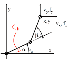
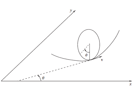
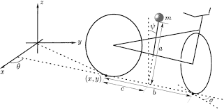
Example 2.16 A rigid rotation of the system of particles consists in a rotation of all vectors of the system through the same angle $\delta \theta$ about an axis defined by the unit vector $\hat{\mathbf{n}}$. Inspecting Fig. 2.7 one infers that $\left|\delta \mathbf{r}_i\right|=r_i \sin \alpha \delta \theta$, which has the appearence of magnitude of a vector product. In fact, defining the vector $\delta \theta=\delta \theta \hat{\mathbf{n}}$, it follows at once that the correct expression for the vector $\delta \mathbf{r}_i$ is $\delta \mathbf{r}_i=\delta \theta \times \mathbf{r}_i$. Since each velocity $\delta \mathbf{v}_i$ undergoes the same rotation, equations (2.131) are valid with
$$
\delta \mathbf{r}_i=\delta \theta \times \mathbf{r}_i, \quad \delta \mathbf{v}_i=\delta \theta \times \mathbf{v}_i, \quad \text { (rotation) }
$$
where $\delta \theta$ is the infinitesimal parameter associated with the transformation.

物理代写|分析力学代写Analytical Mechanics代考|Conservation Theorems

In order to state the results in a sufficiently general form, let us assume that the system described by the Lagrangian (2.132) is subject to the holonomic constraints
$$
f_s\left(\mathbf{r}1, \ldots, \mathbf{r}_N, t\right)=0, \quad s=1, \ldots, p . $$ Theorem 2.5.2 Let a mechanical system be described by the Lagrangian $L=T-V$, where $V$ is a velocity-independent potential. If the Lagrangian and the constraints (2.137) are invariant under an arbitrary rigid translation, then the total linear momentum of the system is conserved. Proof According to the discussion at the end of Section 2.4, the Lagrangian $$ \mathcal{L}=L(\mathbf{r}, \mathbf{v}, t)+\sum{s=1}^p \lambda_s f_s(\mathbf{r}, t)
$$
yields, in one fell swoop, the equations of motion and the constraint equations. Since $L$ and the constraint equations are invariant under arbitrary translations, so is $\mathcal{L}$. In particular, $\mathcal{L}$ is invariant under any infinitesimal translation and we have
$$
0=\delta \mathcal{L}=\sum_{i=1}^N \frac{\partial \mathcal{L}}{\partial \mathbf{r}i} \cdot(\epsilon \hat{\mathbf{n}})=\epsilon \hat{\mathbf{n}} \cdot \sum{i=1}^N \frac{\partial \mathcal{L}}{\partial \mathbf{r}i}, $$ where we have used (2.133) and (2.135). Since $\epsilon$ is arbitrary, we obtain $$ \hat{\mathbf{n}} \cdot \sum{i=1}^N \frac{\partial \mathcal{L}}{\partial \mathbf{r}_i}=0
$$
Noting that
$$
\frac{\partial \mathcal{L}}{\partial \mathbf{v}_i} \equiv \frac{\partial \mathcal{L}}{\partial \dot{\mathbf{r}}_i}=\frac{\partial L}{\partial \dot{\mathbf{r}}_i}=m_i \dot{\mathbf{r}}_i=\mathbf{p}_i,
$$
where $\mathbf{p}_i$ is the linear momentum of the $i$ th particle, Lagrange’s equations can be written in the form
$$
\frac{\partial \mathcal{L}}{\partial \mathbf{r}_i}=\frac{d}{d t}\left(\frac{\partial \mathcal{L}}{\partial \dot{\mathbf{r}}_i}\right)=\frac{d \mathbf{p}_i}{d t}
$$

分析力学代考

物理代写|分析力学代写Analytical Mechanics代考|Infinitesimal Translations and Rotations

考虑无穷小变换
$$
\mathbf{r} i \rightarrow \mathbf{r}_i^{\prime}=\mathbf{r}_i+\delta \mathbf{r}_i, \quad \mathbf{v}_i \rightarrow \mathbf{v}_i^{\prime}=\mathbf{v}_i+\delta \mathbf{v}_i
$$
在哪里 $\delta \mathbf{r}_i$ 和 $\delta \mathbf{v}_i$ 是一个系统的位置和速度的无穷小位移 $N$ 粒子。让
$$
L\left(\mathbf{r}_1, \ldots, \mathbf{r}_N, \dot{\mathbf{r}}_1, \ldots, \dot{\mathbf{r}}_N, t\right) \equiv L(\mathbf{r}, \mathbf{v}, t)
$$
是系统的拉格朗日量。的变化 $L$ 变换下 (2.131) 定义为
$$
\delta L=L\left(\mathbf{r}^{\prime}, \mathbf{v}^{\prime}, t\right)-L(\mathbf{r}, \mathbf{v}, t)=\sum i=1^N\left[\frac{\partial L}{\partial \mathbf{r}_i} \cdot \delta \mathbf{r}_i+\frac{\partial L}{\partial \mathbf{v}_i} \cdot \delta \mathbf{v}_i\right]
$$
我们在哪里使用了符号
$$
\frac{\partial L}{\partial \mathbf{r}_i} \equiv \frac{\partial L}{\partial x_i} \hat{\mathbf{x}}+\frac{\partial L}{\partial y_i} \hat{\mathbf{y}}+\frac{\partial L}{\partial z_i} \hat{\mathbf{z}}
$$
具有类似的定义 $\partial L / \partial \mathbf{v}_i$.
示例 2.15 粒子系统的刚性平移包含相同的位移 $\boldsymbol{\epsilon}=\epsilon \hat{\mathbf{n}}$ 系统的所有粒子，因此速度以及粒子的相对位置 保持不变。在这种情况下，等式 (2.131) 是有效的
$$
\delta \mathbf{r}_i=\epsilon \hat{\mathbf{n}}, \quad \delta \mathbf{v}_i=0, \quad(\text { translation })
$$
在哪里 $\epsilon$ 是具有长度维度的无穷小参数。
示例 2.16 粒子系统的刚性旋转包括系统的所有矢量旋转相同的角度 $\delta \theta$ 关于由单位向量定义的轴 $\hat{\mathbf{n}}$. 检查 图 2.7 可以推断出 $\left|\delta \mathbf{r}_i\right|=r_i \sin \alpha \delta \theta$ ，它具有矢量积的大小。事实上，定义向量 $\delta \theta=\delta \theta \hat{\mathbf{n}}$, 立即得出 向量的正确表达式 $\delta \mathbf{r}_i$ 是 $\delta \mathbf{r}_i=\delta \theta \times \mathbf{r}_i$. 由于每个速度 $\delta \mathbf{v}_i$ 经历相同的旋转，方程 (2.131) 是有效的
$$
\delta \mathbf{r}_i=\delta \theta \times \mathbf{r}_i, \quad \delta \mathbf{v}_i=\delta \theta \times \mathbf{v}_i, \quad \text { (rotation) }
$$
在哪里 $\delta \theta$ 是与变换相关联的无穷小参数。

物理代写|分析力学代写Analytical Mechanics代考|Conservation Theorems

为了以足够一般的形式陈述结果，让我们假设拉格朗日 (2.132) 描述的系统受制于完整约束
$$
f_s\left(\mathbf{r} 1, \ldots, \mathbf{r}N, t\right)=0, \quad s=1, \ldots, p . $$ 定理 2.5.2 让机械系统用拉格朗日量描述 $L=T-V$ ，在哪里 $V$ 是与速度无关的势能。如果拉格朗日量 和约束 (2.137) 在任意刚性平移下不变，则系统的总线性动量守恒。证明 根据 2.4 节末尾的讨论，拉格朗 日量 $$ \mathcal{L}=L(\mathbf{r}, \mathbf{v}, t)+\sum s=1^p \lambda_s f_s(\mathbf{r}, t) $$ 一举得出运动方程和约束方程。自从 $L$ 并且约束方程在任意平移下是不变的，因此是 $\mathcal{L}$. 尤其， $\mathcal{L}$ 在任何 无穷小平移下都是不变的，我们有 $$ 0=\delta \mathcal{L}=\sum{i=1}^N \frac{\partial \mathcal{L}}{\partial \mathbf{r} i} \cdot(\epsilon \hat{\mathbf{n}})=\epsilon \hat{\mathbf{n}} \cdot \sum i=1^N \frac{\partial \mathcal{L}}{\partial \mathbf{r} i},
$$
我们使用 (2.133) 和 (2.135) 的地方。自从 $\epsilon$ 是任意的，我们得到
$$
\hat{\mathbf{n}} \cdot \sum i=1^N \frac{\partial \mathcal{L}}{\partial \mathbf{r}_i}=0
$$
注意到
$$
\frac{\partial \mathcal{L}}{\partial \mathbf{v}_i} \equiv \frac{\partial \mathcal{L}}{\partial \dot{\mathbf{r}}_i}=\frac{\partial L}{\partial \dot{\mathbf{r}}_i}=m_i \dot{\mathbf{r}}_i=\mathbf{p}_i
$$
在哪里 $\mathbf{p}_i$ 是线性动量 $i$ th 粒子，拉格朗日方程可以写成以下形式
$$
\frac{\partial \mathcal{L}}{\partial \mathbf{r}_i}=\frac{d}{d t}\left(\frac{\partial \mathcal{L}}{\partial \dot{\mathbf{r}}_i}\right)=\frac{d \mathbf{p}_i}{d t}
$$

统计代写请认准statistics-lab™. statistics-lab™为您的留学生涯保驾护航。

金融工程代写

金融工程是使用数学技术来解决金融问题。金融工程使用计算机科学、统计学、经济学和应用数学领域的工具和知识来解决当前的金融问题，以及设计新的和创新的金融产品。

非参数统计代写

非参数统计指的是一种统计方法，其中不假设数据来自于由少数参数决定的规定模型；这种模型的例子包括正态分布模型和线性回归模型。

广义线性模型代考

广义线性模型（GLM）归属统计学领域，是一种应用灵活的线性回归模型。该模型允许因变量的偏差分布有除了正态分布之外的其它分布。

术语 广义线性模型（GLM）通常是指给定连续和/或分类预测因素的连续响应变量的常规线性回归模型。它包括多元线性回归，以及方差分析和方差分析（仅含固定效应）。

有限元方法代写

有限元方法（FEM）是一种流行的方法，用于数值解决工程和数学建模中出现的微分方程。典型的问题领域包括结构分析、传热、流体流动、质量运输和电磁势等传统领域。

有限元是一种通用的数值方法，用于解决两个或三个空间变量的偏微分方程（即一些边界值问题）。为了解决一个问题，有限元将一个大系统细分为更小、更简单的部分，称为有限元。这是通过在空间维度上的特定空间离散化来实现的，它是通过构建对象的网格来实现的：用于求解的数值域，它有有限数量的点。边界值问题的有限元方法表述最终导致一个代数方程组。该方法在域上对未知函数进行逼近。[1] 然后将模拟这些有限元的简单方程组合成一个更大的方程系统，以模拟整个问题。然后，有限元通过变化微积分使相关的误差函数最小化来逼近一个解决方案。

tatistics-lab作为专业的留学生服务机构，多年来已为美国、英国、加拿大、澳洲等留学热门地的学生提供专业的学术服务，包括但不限于Essay代写，Assignment代写，Dissertation代写，Report代写，小组作业代写，Proposal代写，Paper代写，Presentation代写，计算机作业代写，论文修改和润色，网课代做，exam代考等等。写作范围涵盖高中，本科，研究生等海外留学全阶段，辐射金融，经济学，会计学，审计学，管理学等全球99%专业科目。写作团队既有专业英语母语作者，也有海外名校硕博留学生，每位写作老师都拥有过硬的语言能力，专业的学科背景和学术写作经验。我们承诺100%原创，100%专业，100%准时，100%满意。

随机分析代写

随机微积分是数学的一个分支，对随机过程进行操作。它允许为随机过程的积分定义一个关于随机过程的一致的积分理论。这个领域是由日本数学家伊藤清在第二次世界大战期间创建并开始的。

时间序列分析代写

随机过程，是依赖于参数的一组随机变量的全体，参数通常是时间。 随机变量是随机现象的数量表现，其时间序列是一组按照时间发生先后顺序进行排列的数据点序列。通常一组时间序列的时间间隔为一恒定值（如1秒，5分钟，12小时，7天，1年），因此时间序列可以作为离散时间数据进行分析处理。研究时间序列数据的意义在于现实中，往往需要研究某个事物其随时间发展变化的规律。这就需要通过研究该事物过去发展的历史记录，以得到其自身发展的规律。

回归分析代写

多元回归分析渐进（Multiple Regression Analysis Asymptotics）属于计量经济学领域，主要是一种数学上的统计分析方法，可以分析复杂情况下各影响因素的数学关系，在自然科学、社会和经济学等多个领域内应用广泛。

MATLAB代写

MATLAB 是一种用于技术计算的高性能语言。它将计算、可视化和编程集成在一个易于使用的环境中，其中问题和解决方案以熟悉的数学符号表示。典型用途包括：数学和计算算法开发建模、仿真和原型制作数据分析、探索和可视化科学和工程图形应用程序开发，包括图形用户界面构建MATLAB 是一个交互式系统，其基本数据元素是一个不需要维度的数组。这使您可以解决许多技术计算问题，尤其是那些具有矩阵和向量公式的问题，而只需用 C 或 Fortran 等标量非交互式语言编写程序所需的时间的一小部分。MATLAB 名称代表矩阵实验室。MATLAB 最初的编写目的是提供对由 LINPACK 和 EISPACK 项目开发的矩阵软件的轻松访问，这两个项目共同代表了矩阵计算软件的最新技术。MATLAB 经过多年的发展，得到了许多用户的投入。在大学环境中，它是数学、工程和科学入门和高级课程的标准教学工具。在工业领域，MATLAB 是高效研究、开发和分析的首选工具。MATLAB 具有一系列称为工具箱的特定于应用程序的解决方案。对于大多数 MATLAB 用户来说非常重要，工具箱允许您学习和应用专业技术。工具箱是 MATLAB 函数（M 文件）的综合集合，可扩展 MATLAB 环境以解决特定类别的问题。可用工具箱的领域包括信号处理、控制系统、神经网络、模糊逻辑、小波、仿真等。

R语言代写	问卷设计与分析代写
PYTHON代写	回归分析与线性模型代写
MATLAB代写	方差分析与试验设计代写
STATA代写	机器学习/统计学习代写
SPSS代写	计量经济学代写
EVIEWS代写	时间序列分析代写
EXCEL代写	深度学习代写
SQL代写	各种数据建模与可视化代写

如果你也在 怎样代写分析力学Analytical Mechanics这个学科遇到相关的难题，请随时右上角联系我们的24/7代写客服。

分析力学是理论力学的一个分支，是对经典力学的高度数学化的表达。

statistics-lab™ 为您的留学生涯保驾护航 在代写分析力学Analytical Mechanics方面已经树立了自己的口碑, 保证靠谱, 高质且原创的统计Statistics代写服务。我们的专家在代写分析力学Analytical Mechanics代写方面经验极为丰富，各种代写分析力学Analytical Mechanics相关的作业也就用不着说。

我们提供的分析力学Analytical Mechanics及其相关学科的代写，服务范围广, 其中包括但不限于:

• Statistical Inference 统计推断
• Statistical Computing 统计计算
• Advanced Probability Theory 高等概率论
• Advanced Mathematical Statistics 高等数理统计学
• (Generalized) Linear Models 广义线性模型
• Statistical Machine Learning 统计机器学习
• Longitudinal Data Analysis 纵向数据分析
• Foundations of Data Science 数据科学基础

物理代写|分析力学代写Analytical Mechanics代考|Holonomic Constraints and Lagrange Multipliers

Although equations of the form (2.75) do not include the most general non-holonomic constraints, they do include the holonomic ones. Indeed, holonomic constraints take the form
$$
f_i(q, t)=0, \quad l=1, \ldots, p
$$
hence, by taking the total time derivative,
$$
\sum_{k=1}^n \frac{\partial f_i}{\partial q_k} \dot{q}_k+\frac{\partial f_l}{\partial t}=0, \quad l=1, \ldots, p
$$

These equations are of the form (2.75) with
$$
a_{l k}=\frac{\partial f_l}{\partial q_k}, \quad a_{l t}=\frac{\partial f_l}{\partial t} .
$$
Thus, the Lagrange multiplier method can be applied to holonomic systems when it is inconvenient to replace the $q$ s by a smaller set of independent variables or when one wishes to determine the constraint forces. By way of illustration, let us apply the Lagrange multiplier formalism to a holonomic case.

In the holonomic case it is possible to choose generalised coordinates in terms of which the constraint equations are identically satisfied. Nevertheless, in the discussion of certain general theoretical questions it is sometimes advantageous to use an excessive number of coordinates and treat the holonomic constraints by the Lagrange multiplier technique. Given the holonomic constraints (2.96), consider the new Lagrangian $\mathcal{L}$ defined by
$$
\mathcal{L}=L(q, \dot{q}, t)+\sum_{l=1}^p \lambda_l f_l(q, t) .
$$
Introducing the $n+p$ variables $\xi_1, \ldots, \xi_{n+p}$ defined by
$$
\xi_1=q_1, \ldots, \xi_n=q_n, \xi_{n+1}=\lambda_1, \ldots, \xi_{n+p}=\lambda_p
$$
and treating them as $n+p$ independent generalised coordinates, the equations of motion and the constraint equations can be written in one fell swoop as
$$
\frac{d}{d t}\left(\frac{\partial \mathcal{L}}{\partial \dot{\xi}_k}\right)-\frac{\partial \mathcal{L}}{\partial \xi_k}=0, \quad k=1, \ldots, n+p
$$

物理代写|分析力学代写Analytical Mechanics代考|Constants of the Motion

A constant of the motion is a conserved physical quantity – that is, a quantity associated with a mechanical system whose value does not change during the dynamical evolution of the system. Mathematically, a constant of the motion, an invariant, a first integral or simply an integral of a mechanichal system is a function $f$ of the coordinates, velocities and, possibly, time that remains constant throughout the motion of the system:
$$
\frac{d f}{d t}=0 \quad \text { or } \quad f\left(q_1(t), \ldots, q_n(t), \dot{q}_1(t), \ldots, \dot{q}_n(t), t\right)=\text { constant }
$$
where the functions $q_k(t)$ satisfy the equations of motion for the system.
Example 2.10 In the case of a harmonic oscillator with angular frequency $\omega$,
$$
f(x, \dot{x}, t)=\arctan \left(\frac{\omega x}{\dot{x}}\right)-\omega t
$$
is a constant of the motion. In order to check this claim we have to compute the total time derivative of $f$, which is given by
$$
\frac{d f}{d t}=\frac{\partial f}{\partial x} \frac{d x}{d t}+\frac{\partial f}{\partial \dot{x}} \frac{d \dot{x}}{d t}+\frac{\partial f}{\partial t}=\frac{1}{1+\omega^2 x^2 / \dot{x}^2} \frac{\omega}{\dot{x}} \dot{x}+\frac{1}{1+\omega^2 x^2 / \dot{x}^2}\left[-\frac{\omega x}{\dot{x}^2}\right] \ddot{x}-\omega .
$$
Using the oscillator equation of motion, $\ddot{x}=-\omega^2 x$, Eq. (2.122) reduces to
$$
\frac{d f}{d t}=\omega \frac{1+\omega^2 x^2 / \dot{x}^2}{1+\omega^2 x^2 / \dot{x}^2}-\omega=\omega-\omega=0
$$
and $f$ is indeed a constant of the motion.
Constants of the motion supply first-order differential equations that give important information about the time evolution of the system. Even though the exact solution to the equations of motion may be unknown, the knowledge of certain first integrals often reveals physically relevant facts regarding the nature of the motion. Sometimes it is possible to obtain exact answers to certain questions thanks to the constants of the motion, without having to completely solve the dynamical problem. Therefore, investigating general conditions that ensure the existence of constants of the motion is highly relevant. The first and simplest result of such an investigation will be stated after two useful definitions.

分析力学代考

物理代写|分析力学代写Analytical Mechanics代考|Holonomic Constraints and Lagrange Multipliers

尽管形式 (2.75) 的方程不包括最一般的非完整约束，但它们确实包括完整约束。事实上，完整约束采取 的形式
$$
f_i(q, t)=0, \quad l=1, \ldots, p
$$
因此，通过取总时间导数，
$$
\sum_{k=1}^n \frac{\partial f_i}{\partial q_k} \dot{q}k+\frac{\partial f_l}{\partial t}=0, \quad l=1, \ldots, p $$ 这些方程的形式为 (2.75)，其中 $$ a{l k}=\frac{\partial f_l}{\partial q_k}, \quad a_{l t}=\frac{\partial f_l}{\partial t}
$$
因此，当不方便替换 $q$ s 通过一组较小的自变量或当人们希望确定约束力时。作为说明，让我们将拉格朗 日乘数形式应用于完整情况。
在完整的情况下，可以选择广义坐标，根据该广义坐标，约束方程被相同地满足。然而，在讨论某些一 般性理论问题时，有时使用过多的坐标并通过拉格朗日乘子技术处理完整约束是有利的。给定完整约束 (2.96)，考虑新的拉格朗日 $\mathcal{L}$ 被定义为
$$
\mathcal{L}=L(q, \dot{q}, t)+\sum_{l=1}^p \lambda_l f_l(q, t)
$$
介绍 $n+p$ 变量 $\xi_1, \ldots, \xi_{n+p}$ 被定义为
$$
\xi_1=q_1, \ldots, \xi_n=q_n, \xi_{n+1}=\lambda_1, \ldots, \xi_{n+p}=\lambda_p
$$
并将它们视为 $n+p$ 独立的广义坐标，运动方程和约束方程可以一举写成
$$
\frac{d}{d t}\left(\frac{\partial \mathcal{L}}{\partial \dot{\xi}_k}\right)-\frac{\partial \mathcal{L}}{\partial \xi_k}=0, \quad k=1, \ldots, n+p
$$

物理代写|分析力学代写Analytical Mechanics代考|Constants of the Motion

运动常数是守恒的物理量，即与机械系统相关的量，其值在系统的动态演化过程中不会改变。在数学 上，运动常数、不变量、第一个积分或机械系统的简单积分是一个函数 $f$ 在整个系统运动过程中保持恒定 的坐标、速度和可能的时间:
$$
\frac{d f}{d t}=0 \quad \text { or } \quad f\left(q_1(t), \ldots, q_n(t), \dot{q}_1(t), \ldots, \dot{q}_n(t), t\right)=\text { constant }
$$
功能在哪里 $q_k(t)$ 满足系统的运动方程。
示例 2.10 在具有角频率的谐振子的情况下 $\omega$ ，
$$
f(x, \dot{x}, t)=\arctan \left(\frac{\omega x}{\dot{x}}\right)-\omega t
$$
是运动的常数。为了验证这个说法，我们必须计算总时间导数 $f$ ，这是由
$$
\frac{d f}{d t}=\frac{\partial f}{\partial x} \frac{d x}{d t}+\frac{\partial f}{\partial \dot{x}} \frac{d \dot{x}}{d t}+\frac{\partial f}{\partial t}=\frac{1}{1+\omega^2 x^2 / \dot{x}^2} \frac{\omega}{\dot{x}} \dot{x}+\frac{1}{1+\omega^2 x^2 / \dot{x}^2}\left[-\frac{\omega x}{\dot{x}^2}\right] \ddot{x}-\omega
$$
使用振荡器运动方程， $\ddot{x}=-\omega^2 x$ ，当量。(2.122)简化为
$$
\frac{d f}{d t}=\omega \frac{1+\omega^2 x^2 / \dot{x}^2}{1+\omega^2 x^2 / \dot{x}^2}-\omega=\omega-\omega=0
$$
和 $f$ 确实是运动的常数。
运动常数提供一阶微分方程，提供有关系统时间演化的重要信息。尽管运动方程的精确解可能是末知 的，但某些一阶积分的知识通常揭示了关于运动性质的物理相关事实。有时，由于运动的常数，有可能 获得某些问题的准确答案，而不必完全解决动力学问题。因此，研究确保运动常数存在的一般条件是高 度相关的。这种调查的第一个也是最简单的结果将在两个有用的定义之后说明。

统计代写请认准statistics-lab™. statistics-lab™为您的留学生涯保驾护航。

金融工程代写

金融工程是使用数学技术来解决金融问题。金融工程使用计算机科学、统计学、经济学和应用数学领域的工具和知识来解决当前的金融问题，以及设计新的和创新的金融产品。

非参数统计代写

非参数统计指的是一种统计方法，其中不假设数据来自于由少数参数决定的规定模型；这种模型的例子包括正态分布模型和线性回归模型。

广义线性模型代考

广义线性模型（GLM）归属统计学领域，是一种应用灵活的线性回归模型。该模型允许因变量的偏差分布有除了正态分布之外的其它分布。

术语 广义线性模型（GLM）通常是指给定连续和/或分类预测因素的连续响应变量的常规线性回归模型。它包括多元线性回归，以及方差分析和方差分析（仅含固定效应）。

有限元方法代写

有限元方法（FEM）是一种流行的方法，用于数值解决工程和数学建模中出现的微分方程。典型的问题领域包括结构分析、传热、流体流动、质量运输和电磁势等传统领域。

有限元是一种通用的数值方法，用于解决两个或三个空间变量的偏微分方程（即一些边界值问题）。为了解决一个问题，有限元将一个大系统细分为更小、更简单的部分，称为有限元。这是通过在空间维度上的特定空间离散化来实现的，它是通过构建对象的网格来实现的：用于求解的数值域，它有有限数量的点。边界值问题的有限元方法表述最终导致一个代数方程组。该方法在域上对未知函数进行逼近。[1] 然后将模拟这些有限元的简单方程组合成一个更大的方程系统，以模拟整个问题。然后，有限元通过变化微积分使相关的误差函数最小化来逼近一个解决方案。

tatistics-lab作为专业的留学生服务机构，多年来已为美国、英国、加拿大、澳洲等留学热门地的学生提供专业的学术服务，包括但不限于Essay代写，Assignment代写，Dissertation代写，Report代写，小组作业代写，Proposal代写，Paper代写，Presentation代写，计算机作业代写，论文修改和润色，网课代做，exam代考等等。写作范围涵盖高中，本科，研究生等海外留学全阶段，辐射金融，经济学，会计学，审计学，管理学等全球99%专业科目。写作团队既有专业英语母语作者，也有海外名校硕博留学生，每位写作老师都拥有过硬的语言能力，专业的学科背景和学术写作经验。我们承诺100%原创，100%专业，100%准时，100%满意。

随机分析代写

随机微积分是数学的一个分支，对随机过程进行操作。它允许为随机过程的积分定义一个关于随机过程的一致的积分理论。这个领域是由日本数学家伊藤清在第二次世界大战期间创建并开始的。

时间序列分析代写

随机过程，是依赖于参数的一组随机变量的全体，参数通常是时间。 随机变量是随机现象的数量表现，其时间序列是一组按照时间发生先后顺序进行排列的数据点序列。通常一组时间序列的时间间隔为一恒定值（如1秒，5分钟，12小时，7天，1年），因此时间序列可以作为离散时间数据进行分析处理。研究时间序列数据的意义在于现实中，往往需要研究某个事物其随时间发展变化的规律。这就需要通过研究该事物过去发展的历史记录，以得到其自身发展的规律。

回归分析代写

多元回归分析渐进（Multiple Regression Analysis Asymptotics）属于计量经济学领域，主要是一种数学上的统计分析方法，可以分析复杂情况下各影响因素的数学关系，在自然科学、社会和经济学等多个领域内应用广泛。

MATLAB代写

MATLAB 是一种用于技术计算的高性能语言。它将计算、可视化和编程集成在一个易于使用的环境中，其中问题和解决方案以熟悉的数学符号表示。典型用途包括：数学和计算算法开发建模、仿真和原型制作数据分析、探索和可视化科学和工程图形应用程序开发，包括图形用户界面构建MATLAB 是一个交互式系统，其基本数据元素是一个不需要维度的数组。这使您可以解决许多技术计算问题，尤其是那些具有矩阵和向量公式的问题，而只需用 C 或 Fortran 等标量非交互式语言编写程序所需的时间的一小部分。MATLAB 名称代表矩阵实验室。MATLAB 最初的编写目的是提供对由 LINPACK 和 EISPACK 项目开发的矩阵软件的轻松访问，这两个项目共同代表了矩阵计算软件的最新技术。MATLAB 经过多年的发展，得到了许多用户的投入。在大学环境中，它是数学、工程和科学入门和高级课程的标准教学工具。在工业领域，MATLAB 是高效研究、开发和分析的首选工具。MATLAB 具有一系列称为工具箱的特定于应用程序的解决方案。对于大多数 MATLAB 用户来说非常重要，工具箱允许您学习和应用专业技术。工具箱是 MATLAB 函数（M 文件）的综合集合，可扩展 MATLAB 环境以解决特定类别的问题。可用工具箱的领域包括信号处理、控制系统、神经网络、模糊逻辑、小波、仿真等。

R语言代写	问卷设计与分析代写
PYTHON代写	回归分析与线性模型代写
MATLAB代写	方差分析与试验设计代写
STATA代写	机器学习/统计学习代写
SPSS代写	计量经济学代写
EVIEWS代写	时间序列分析代写
EXCEL代写	深度学习代写
SQL代写	各种数据建模与可视化代写

如果你也在 怎样代写分析力学Analytical Mechanics这个学科遇到相关的难题，请随时右上角联系我们的24/7代写客服。

分析力学是理论力学的一个分支，是对经典力学的高度数学化的表达。

statistics-lab™ 为您的留学生涯保驾护航 在代写分析力学Analytical Mechanics方面已经树立了自己的口碑, 保证靠谱, 高质且原创的统计Statistics代写服务。我们的专家在代写分析力学Analytical Mechanics代写方面经验极为丰富，各种代写分析力学Analytical Mechanics相关的作业也就用不着说。

我们提供的分析力学Analytical Mechanics及其相关学科的代写，服务范围广, 其中包括但不限于:

• Statistical Inference 统计推断
• Statistical Computing 统计计算
• Advanced Probability Theory 高等概率论
• Advanced Mathematical Statistics 高等数理统计学
• (Generalized) Linear Models 广义线性模型
• Statistical Machine Learning 统计机器学习
• Longitudinal Data Analysis 纵向数据分析
• Foundations of Data Science 数据科学基础

物理代写|分析力学代写Analytical Mechanics代考|Virtual Work

The importance of introducing the notion of virtual displacement stems from the following observation: if the surface to which the particle is confined is ideally smooth, the contact force of the surface on the particle, which is the constraint force, has no tangential component and therefore is normal to the surface. Thus, the work done by the constraint force as the particle undergoes a virtual displacement is zero even if the surface is in mótion, differently from thé work donne during a reeal displaccement, which does nôt necessarily vanish. In most physically interesting cases, the total virtual work of the constraint forces is zero, as the next examples attest.

Example 1.10 Two particles joined by a rigid rod move in space. Let $\mathbf{f}_1$ and $\mathbf{f}_2$ be the constraint forces on the particles. By Newton’s third law $\mathbf{f}_1=-\mathbf{f}_2$ with both $\mathbf{f}_1$ and $\mathbf{f}_2$ parallel to the line connecting the particles. The virtual work done by the constraint forces is
$$
\delta W_v=\mathbf{f}_1 \cdot \delta \mathbf{r}_1+\mathbf{f}_2 \cdot \delta \mathbf{r}_2=\mathbf{f}_2 \cdot\left(\delta \mathbf{r}_2-\delta \mathbf{r}_1\right) .
$$
Setting $\mathbf{r}=\mathbf{r}_2-\mathbf{r}_1$, the constraint equation takes the form (1.38), namely $r^2-l^2=0$. In terms of the variable $\mathbf{r}$, the situation is equivalent to the one discussed in Example 1.9. Taking $f(\mathbf{r}, t)=r^2-l^2$, Eq. (1.51) reduces to $\mathbf{r} \cdot \delta \mathbf{r}=0$. Since $\mathbf{f}_2$ and $\mathbf{r}$ are collinear, there exists a scalar $\lambda$ such that $\mathbf{f}_2=\lambda \mathbf{r}$, hence $\delta W_v=\lambda \mathbf{r} \cdot \delta \mathbf{r}=0$. Inasmuch as a rigid body consists of a vast number of particles whose mutual distances are invariable, one concludes that the total virtual work done by the forces responsible for the body’s rigidity is zero.

Example 1.11 A rigid body rolls without slipping on a fixed surface. As a rule, in order to prevent slipping, a friction force between the fixed surface and the surface of the body is needed, that is, the surfaces in contact must be rough. Upon rolling without slipping, the body’s particles at each instant are rotating about an axis that contains the body’s point of contact with the surface. Thus, the friction force acts on a point of the body whose velocity at each instant is zero, because it is on the instantaneous axis of rotation. Virtual displacements are such that the body does not slip on the surface, that is, $\delta \mathbf{r}=0$ at the point of contact between the body and the fixed surface. Therefore, the virtual work done by the constraint force is $\delta W_v=\mathbf{f} \cdot \delta \mathbf{r}=0$ because $\delta \mathbf{r}=0$, even though $\mathbf{f} \neq 0$.

物理代写|分析力学代写Analytical Mechanics代考|Principle of Virtual Work

Newton’s formulation of mechanics is characterised by the set of differential equations
$$
m_i \ddot{\mathbf{r}}_i=\mathbf{F}_i, \quad i=1, \ldots, N,
$$
where $\mathbf{F}_i$ is the total or resultant force on the $i$ th particle, supposedly a known function of positions, velocities and time. This system of differential equations determines a unique solution for the $\mathbf{r}_i(t)$ once the positions and velocities are specified at an initial instant. ${ }^{10}$
In the presence of constraints, it is patently clear how inconvenient the Newtonian formulation is. First of all, it usually requires the use of more coordinates than are necessary to specify the configuration of the system. When the constraints are holonomic, for instance, the positions $\mathbf{r}_1, \ldots, \mathbf{r}_N$ are not mutually independent, making the Newtonian approach uneconomical by demanding the employment of redundant variables. Furthermore, the total force on the $i$ th particle can be decomposed as
$$
\mathbf{F}_i=\mathbf{F}_i^{(a)}+\mathbf{f}_i,
$$
where $\mathbf{F}_i^{(a)}$ is the applied force and $\mathbf{f}_i$ is the constraint force. In the case of the double pendulum in Example 1.4, $\mathbf{F}_1^{(a)}$ and $\mathbf{F}_2^{(a)}$ are the weights of the particles, whereas $\mathbf{f}_1$ and $\mathbf{f}_2$ are determined by the tensions on the rods or strings. The difficulty here lies in that one does not a priori know how the constraint forces depend on the positions and velocities. What one knows, in fact, are the effects produced by the constraint forces. One may also argue that the applied forces are the true causes of the motion, the constraint forces merely serving to ensure the preservation of the geometric or kinematic restrictions in the course of time. No less important is the fact that Newton’s laws – the second law together with the strong version of the third law – turn out to be incapable of correctly describing the motion of certain constrained systems (Stadler, 1982; Casey, 2014).

For all these reasons, it is highly desirable to obtain a formulation of classical mechanics as parsimonious as possible, namely involving only the applied forces and employing only independent coordinates. We shall soon see that this goal is achieved by the Lagrangian formalism when all constraints are holonomic. As an intermediate step towards Lagrange’s formulation, we shall discuss d’Alembert’s principle, which is a method of writing down the equations of motion in terms of the applied forces alone, the derivation of which explores the fact that the virtual work of the constraint forces is zero.

分析力学代考

物理代写|分析力学代写分析力学代考|虚拟功

.

引入虚位移概念的重要性来源于以下观察结果:如果质点所受限制的表面是理想光滑的，则表面对质点的接触力，即约束力，没有切向分量，因此垂直于表面。因此，当粒子经历虚位移时，约束力所做的功为零，即使表面在mótion，这与真实位移时所做的thé功不同，真实位移时所做的功nôt必然消失。在大多数物理上有趣的情况下，约束力的总虚功为零，正如下面的例子所证明的

两个由刚性杆连接的粒子在空间中运动。设$\mathbf{f}_1$和$\mathbf{f}_2$是对粒子的约束力。根据牛顿第三定律$\mathbf{f}_1=-\mathbf{f}_2$$\mathbf{f}_1$和$\mathbf{f}_2$都平行于连接粒子的直线。约束力所做的虚功为
$$
\delta W_v=\mathbf{f}_1 \cdot \delta \mathbf{r}_1+\mathbf{f}_2 \cdot \delta \mathbf{r}_2=\mathbf{f}_2 \cdot\left(\delta \mathbf{r}_2-\delta \mathbf{r}_1\right) .
$$
设$\mathbf{r}=\mathbf{r}_2-\mathbf{r}_1$，约束方程为(1.38)形式，即$r^2-l^2=0$。对于变量$\mathbf{r}$，情况等价于例1.9中讨论的情况。取$f(\mathbf{r}, t)=r^2-l^2$，式(1.51)化简为$\mathbf{r} \cdot \delta \mathbf{r}=0$。由于$\mathbf{f}_2$和$\mathbf{r}$共线，存在一个标量$\lambda$使得$\mathbf{f}_2=\lambda \mathbf{r}$，因此$\delta W_v=\lambda \mathbf{r} \cdot \delta \mathbf{r}=0$。由于刚体由大量相互距离不变的粒子组成，因此可以得出结论，使刚体具有刚性的力所作的虚功的总和为零

刚体在固定表面上滚动而不打滑。一般来说，为了防止打滑，固定表面和物体表面之间需要有摩擦力，即接触的表面必须是粗糙的。在不打滑地滚动时，物体的粒子在每个瞬间都绕着包含物体与表面接触点的轴旋转。因此，摩擦力作用在物体上的一个点上，它的速度在每一刻都为零，因为它在瞬时旋转轴上。虚位移是这样的，使物体在表面上不滑动，即$\delta \mathbf{r}=0$在物体和固定表面之间的接触点。因此，约束力所做的虚功是$\delta W_v=\mathbf{f} \cdot \delta \mathbf{r}=0$，因为$\delta \mathbf{r}=0$，即使$\mathbf{f} \neq 0$ .

物理代写|分析力学代写分析力学代考|虚功原理

牛顿的力学公式的特征是一组微分方程
$$
m_i \ddot{\mathbf{r}}_i=\mathbf{F}_i, \quad i=1, \ldots, N,
$$
，其中$\mathbf{F}_i$是作用在第$i$个粒子上的总力或合力，应该是位置、速度和时间的已知函数。这个微分方程组确定了$\mathbf{r}_i(t)$的唯一解，一旦在初始瞬间指定了位置和速度。${ }^{10}$
在存在约束条件的情况下，很明显牛顿公式是多么不方便。首先，它通常需要使用比指定系统配置所需的更多的坐标。例如，当约束是完整的，位置$\mathbf{r}_1, \ldots, \mathbf{r}_N$不是相互独立的，这使得牛顿方法不经济，因为它要求使用冗余变量。此外，第$i$个粒子上的总力可以分解为
$$
\mathbf{F}_i=\mathbf{F}_i^{(a)}+\mathbf{f}_i,
$$
，其中$\mathbf{F}_i^{(a)}$为施加力，$\mathbf{f}_i$为约束力。在例1.4中的双摆的情况下，$\mathbf{F}_1^{(a)}$和$\mathbf{F}_2^{(a)}$是粒子的重量，而$\mathbf{f}_1$和$\mathbf{f}_2$是由杆或弦上的张力决定的。这里的困难在于，我们不能先验地知道约束力如何依赖于位置和速度。事实上，我们所知道的是约束力所产生的效应。人们也可以争辩说，施加的力是运动的真正原因，约束力仅仅是为了确保在时间过程中几何或运动限制的保存。同样重要的是，牛顿定律——第二定律和第三定律的强版本——被证明不能正确描述某些受约束系统的运动(Stadler, 1982;Casey, 2014)。

由于所有这些原因，得到一个经典力学的公式是非常可取的，即只涉及施加的力和只使用独立的坐标。我们很快就会看到，当所有的约束都是完整的，拉格朗日形式主义就能达到这个目的。作为迈向拉格朗日公式的中间步骤，我们将讨论达朗伯特原理，这是一种仅根据施加的力来写下运动方程的方法，它的推导探讨了约束力的虚功为零的事实

统计代写请认准statistics-lab™. statistics-lab™为您的留学生涯保驾护航。

金融工程代写

金融工程是使用数学技术来解决金融问题。金融工程使用计算机科学、统计学、经济学和应用数学领域的工具和知识来解决当前的金融问题，以及设计新的和创新的金融产品。

非参数统计代写

非参数统计指的是一种统计方法，其中不假设数据来自于由少数参数决定的规定模型；这种模型的例子包括正态分布模型和线性回归模型。

广义线性模型代考

广义线性模型（GLM）归属统计学领域，是一种应用灵活的线性回归模型。该模型允许因变量的偏差分布有除了正态分布之外的其它分布。

术语 广义线性模型（GLM）通常是指给定连续和/或分类预测因素的连续响应变量的常规线性回归模型。它包括多元线性回归，以及方差分析和方差分析（仅含固定效应）。

有限元方法代写

有限元方法（FEM）是一种流行的方法，用于数值解决工程和数学建模中出现的微分方程。典型的问题领域包括结构分析、传热、流体流动、质量运输和电磁势等传统领域。

有限元是一种通用的数值方法，用于解决两个或三个空间变量的偏微分方程（即一些边界值问题）。为了解决一个问题，有限元将一个大系统细分为更小、更简单的部分，称为有限元。这是通过在空间维度上的特定空间离散化来实现的，它是通过构建对象的网格来实现的：用于求解的数值域，它有有限数量的点。边界值问题的有限元方法表述最终导致一个代数方程组。该方法在域上对未知函数进行逼近。[1] 然后将模拟这些有限元的简单方程组合成一个更大的方程系统，以模拟整个问题。然后，有限元通过变化微积分使相关的误差函数最小化来逼近一个解决方案。

tatistics-lab作为专业的留学生服务机构，多年来已为美国、英国、加拿大、澳洲等留学热门地的学生提供专业的学术服务，包括但不限于Essay代写，Assignment代写，Dissertation代写，Report代写，小组作业代写，Proposal代写，Paper代写，Presentation代写，计算机作业代写，论文修改和润色，网课代做，exam代考等等。写作范围涵盖高中，本科，研究生等海外留学全阶段，辐射金融，经济学，会计学，审计学，管理学等全球99%专业科目。写作团队既有专业英语母语作者，也有海外名校硕博留学生，每位写作老师都拥有过硬的语言能力，专业的学科背景和学术写作经验。我们承诺100%原创，100%专业，100%准时，100%满意。

随机分析代写

随机微积分是数学的一个分支，对随机过程进行操作。它允许为随机过程的积分定义一个关于随机过程的一致的积分理论。这个领域是由日本数学家伊藤清在第二次世界大战期间创建并开始的。

时间序列分析代写

随机过程，是依赖于参数的一组随机变量的全体，参数通常是时间。 随机变量是随机现象的数量表现，其时间序列是一组按照时间发生先后顺序进行排列的数据点序列。通常一组时间序列的时间间隔为一恒定值（如1秒，5分钟，12小时，7天，1年），因此时间序列可以作为离散时间数据进行分析处理。研究时间序列数据的意义在于现实中，往往需要研究某个事物其随时间发展变化的规律。这就需要通过研究该事物过去发展的历史记录，以得到其自身发展的规律。

回归分析代写

多元回归分析渐进（Multiple Regression Analysis Asymptotics）属于计量经济学领域，主要是一种数学上的统计分析方法，可以分析复杂情况下各影响因素的数学关系，在自然科学、社会和经济学等多个领域内应用广泛。

MATLAB代写

MATLAB 是一种用于技术计算的高性能语言。它将计算、可视化和编程集成在一个易于使用的环境中，其中问题和解决方案以熟悉的数学符号表示。典型用途包括：数学和计算算法开发建模、仿真和原型制作数据分析、探索和可视化科学和工程图形应用程序开发，包括图形用户界面构建MATLAB 是一个交互式系统，其基本数据元素是一个不需要维度的数组。这使您可以解决许多技术计算问题，尤其是那些具有矩阵和向量公式的问题，而只需用 C 或 Fortran 等标量非交互式语言编写程序所需的时间的一小部分。MATLAB 名称代表矩阵实验室。MATLAB 最初的编写目的是提供对由 LINPACK 和 EISPACK 项目开发的矩阵软件的轻松访问，这两个项目共同代表了矩阵计算软件的最新技术。MATLAB 经过多年的发展，得到了许多用户的投入。在大学环境中，它是数学、工程和科学入门和高级课程的标准教学工具。在工业领域，MATLAB 是高效研究、开发和分析的首选工具。MATLAB 具有一系列称为工具箱的特定于应用程序的解决方案。对于大多数 MATLAB 用户来说非常重要，工具箱允许您学习和应用专业技术。工具箱是 MATLAB 函数（M 文件）的综合集合，可扩展 MATLAB 环境以解决特定类别的问题。可用工具箱的领域包括信号处理、控制系统、神经网络、模糊逻辑、小波、仿真等。

R语言代写	问卷设计与分析代写
PYTHON代写	回归分析与线性模型代写
MATLAB代写	方差分析与试验设计代写
STATA代写	机器学习/统计学习代写
SPSS代写	计量经济学代写
EVIEWS代写	时间序列分析代写
EXCEL代写	深度学习代写
SQL代写	各种数据建模与可视化代写

如果你也在 怎样代写分析力学Analytical Mechanics这个学科遇到相关的难题，请随时右上角联系我们的24/7代写客服。

分析力学是理论力学的一个分支，是对经典力学的高度数学化的表达。

statistics-lab™ 为您的留学生涯保驾护航 在代写分析力学Analytical Mechanics方面已经树立了自己的口碑, 保证靠谱, 高质且原创的统计Statistics代写服务。我们的专家在代写分析力学Analytical Mechanics代写方面经验极为丰富，各种代写分析力学Analytical Mechanics相关的作业也就用不着说。

我们提供的分析力学Analytical Mechanics及其相关学科的代写，服务范围广, 其中包括但不限于:

• Statistical Inference 统计推断
• Statistical Computing 统计计算
• Advanced Probability Theory 高等概率论
• Advanced Mathematical Statistics 高等数理统计学
• (Generalized) Linear Models 广义线性模型
• Statistical Machine Learning 统计机器学习
• Longitudinal Data Analysis 纵向数据分析
• Foundations of Data Science 数据科学基础

物理代写|分析力学代写Analytical Mechanics代考|Holonomic Constraints

All of the above constraints are holonomic. If $\xi_1, \ldots, \xi_M$ are arbitrary coordinates employed to describe the configuration ${ }^6$ of a mechanical system, a constraint is said to be holonomic ${ }^7$ if it can be expressed by an equation of the form
$$
f\left(\xi_1, \ldots, \xi_M, t\right)=0,
$$
that is, by a functional relation among the coordinates alone, with a possible explicit time dependence. Constraints that cannot be so represented are said to be non-holonomic. For instance, the requirement that all molecules of a gas remain inside a vessel is described by inequalities: if the vessel is a box with sides $a, b, c$, we have $0<x_i<a, 0<y_i<b$, $0<z_i<c$, where $\mathbf{r}_i=\left(x_i, y_i, z_i\right)$ is the position vector of the $i$ th molecule (treated as a point particle).

Definition 1.2.1 A holonomic system is a mechanical system whose constraints are all of the form (1.41).

There often occur, especially in rigid-body dynamics, constraints that can be represented by equations involving the velocities, that is, differential equations of the form
$$
g\left(\xi_1, \ldots, \xi_M, \dot{\xi}_1, \ldots, \dot{\xi}_M, t\right)=0 .
$$
Example 1.5 A cylinder rolls without slipping on a straight track. With $x$ the position of the cylinder’s centre of mass and $\phi$ the angle of rotation about the centre of mass, the rolling condition is characterised by
$$
\dot{x}=R \dot{\phi},
$$
where $R$ is the cylinder’s radius.
Example 1.6 An upright disc rolls without slipping on a horizontal plane. Let $(x, y)$ be the position of the disc’s centre of mass, $\theta$ be the angle the plane of the disc makes with the $x$-axis, and $\phi$ be the angle of rotation of the disc about its symmetry axis (see Fig. 1.2). With $\mathbf{v}$ the centre-of-mass velocity, the disc rolls without slipping so long as $v=R \dot{\phi}$. Noting that $\dot{x} \equiv v_x=v \cos \theta$ and $\dot{y} \equiv v_y=v \sin \theta$, we are led to the first-order differential equations
$$
\dot{x}-R \dot{\phi} \cos \theta=0, \quad \dot{y}-R \dot{\phi} \sin \theta=0
$$
which mathematically express the rolling condition.

物理代写|分析力学代写Analytical Mechanics代考|Virtual Displacements

Infinitesimal displacements that change a possible configuration into another possible configuration at the same instant are called virtual displacements. More precisely, given a system of $N$ particles, the virtual displacements $\delta \mathbf{r}_i, i=1, \ldots, N$, are infinitesimal displacements from positions $\mathbf{r}_1, \ldots, \mathbf{r}_N$ carried out instantaneously ${ }^9$ and with the property of being compatible with the constraints. In short, the defining attributes of virtual displacements are: (1) they are infinitesimal; (2) they take place at a fixed instant; (3) they do not violate the constraints.

Example 1.9 A particle is confined to a moving surface. Let $f(\mathbf{r}, t)=0$ be the equation of the surface. A virtual displacement must be consistent with the constraint, that is, the point $\mathbf{r}$ and the displaced point $\mathbf{r}+\delta \mathbf{r}$ must belong to the surface at the same time $t$ :
$$
f(\mathbf{r}+\delta \mathbf{r}, t)=0 \Longrightarrow f(\mathbf{r}, t)+\nabla f \cdot \delta \mathbf{r}=0 \Longrightarrow \nabla f \cdot \delta \mathbf{r}=0 .
$$
Since $\nabla f$ is perpendicular to the surface at time $t$, the virtual displacement $\delta \mathbf{r}$ is tangent to the surface at this same instant (Fig. 1.4).

Note, however, that a real displacement $d \mathbf{r}$ takes place during a time interval $d t$. Therefore, in order that the particle remain on the surface, it is necessary that
$$
f(\mathbf{r}+d \mathbf{r}, t+d t)=0 \Longrightarrow \nabla f \cdot d \mathbf{r}+\frac{\partial f}{\partial t} d t=0 .
$$ It is clear that the real displacement $d \mathbf{r}$ is not tangent to the surface as long as $\partial f / \partial t \neq 0$. Only the virtual displacement $\delta \mathbf{r}$ performed at a fixed time is tangent to the surface even if it is moving. Fig. 1.4 illustrates the difference between virtual and real displacements for a particle confined to a surface that moves with velocity $\mathbf{u}$ at instant $t$.

分析力学代考

物理代写|分析力学代写分析力学代考|完整约束

以上所有约束都是完整的。如果$\xi_1, \ldots, \xi_M$是用来描述机械系统构型${ }^6$的任意坐标，那么如果一个约束可以用
$$
f\left(\xi_1, \ldots, \xi_M, t\right)=0,
$$
这样的方程表示，也就是说，通过坐标之间的函数关系，可能具有显式的时间依赖性，那么这个约束就是完整的${ }^7$。不能这样表示的约束称为非完整约束。例如，要求气体的所有分子都留在容器内可以用不等式来描述:如果容器是一个边为$a, b, c$的盒子，我们有$0<x_i<a, 0<y_i<b$, $0<z_i<c$，其中$\mathbf{r}_i=\left(x_i, y_i, z_i\right)$是$i$第th分子的位置向量(作为点粒子处理)

1.2.1完整系统是一个机械系统，它的约束条件都是形式(1.41)

经常出现，特别是在刚体动力学中，可以用涉及速度的方程来表示的约束，即形式为的微分方程$$
g\left(\xi_1, \ldots, \xi_M, \dot{\xi}_1, \ldots, \dot{\xi}_M, t\right)=0 .
$$例1.5圆柱体在直线轨道上滚动时不打滑。用 $x$ 圆柱体质心的位置和 $\phi$ 围绕质心的旋转角度，轧制条件的特征为
$$
\dot{x}=R \dot{\phi},
$$
where $R$ 是圆柱体的半径。
示例1.6竖直磁盘在水平面上滚动时不打滑。让 $(x, y)$ 是圆盘质心的位置， $\theta$ 为圆盘的平面与平面的夹角 $x$-轴，和 $\phi$ 为圆盘绕其对称轴旋转的角度(见图1.2)。用 $\mathbf{v}$ 质量中心速度，圆盘不滑动地滚动，只要 $v=R \dot{\phi}$。注意到 $\dot{x} \equiv v_x=v \cos \theta$ 和 $\dot{y} \equiv v_y=v \sin \theta$，我们得到一阶微分方程
$$
\dot{x}-R \dot{\phi} \cos \theta=0, \quad \dot{y}-R \dot{\phi} \sin \theta=0
$$
，用数学方法表示轧制条件

物理代写|分析力学代写分析力学代考|虚拟位移

.

在同一时刻将一种可能的构型变为另一种可能构型的无穷小位移称为虚位移。更准确地说，给定一个$N$粒子的系统，虚位移$\delta \mathbf{r}_i, i=1, \ldots, N$是来自位置$\mathbf{r}_1, \ldots, \mathbf{r}_N$的无穷小位移，瞬时执行${ }^9$，具有与约束相容的性质。简而言之，虚位移的定义属性是:(1)它们是无穷小的;(2)它们发生在固定的时刻;(3)它们不违反约束。

一个粒子被限制在一个移动的表面上。设$f(\mathbf{r}, t)=0$为曲面的方程。虚位移必须与约束一致，即点$\mathbf{r}$和位移点$\mathbf{r}+\delta \mathbf{r}$必须同时属于曲面$t$:
$$
f(\mathbf{r}+\delta \mathbf{r}, t)=0 \Longrightarrow f(\mathbf{r}, t)+\nabla f \cdot \delta \mathbf{r}=0 \Longrightarrow \nabla f \cdot \delta \mathbf{r}=0 .
$$
由于$\nabla f$在$t$时刻垂直于曲面，所以虚位移$\delta \mathbf{r}$在同一时刻与曲面相切(图1.4)

但是请注意，真正的位移$d \mathbf{r}$发生在$d t$的时间间隔内。因此，为了使粒子保持在表面上，有必要
$$
f(\mathbf{r}+d \mathbf{r}, t+d t)=0 \Longrightarrow \nabla f \cdot d \mathbf{r}+\frac{\partial f}{\partial t} d t=0 .
$$显然，只要$\partial f / \partial t \neq 0$，实位移$d \mathbf{r}$就不与表面相切。只有在固定时间执行的虚拟位移$\delta \mathbf{r}$与表面相切，即使它在移动。图1.4说明了限制在以速度$\mathbf{u}$在瞬间$t$运动的表面上的粒子的虚位移和实位移之间的差异。

统计代写请认准statistics-lab™. statistics-lab™为您的留学生涯保驾护航。

金融工程代写

金融工程是使用数学技术来解决金融问题。金融工程使用计算机科学、统计学、经济学和应用数学领域的工具和知识来解决当前的金融问题，以及设计新的和创新的金融产品。

非参数统计代写

非参数统计指的是一种统计方法，其中不假设数据来自于由少数参数决定的规定模型；这种模型的例子包括正态分布模型和线性回归模型。

广义线性模型代考

广义线性模型（GLM）归属统计学领域，是一种应用灵活的线性回归模型。该模型允许因变量的偏差分布有除了正态分布之外的其它分布。

术语 广义线性模型（GLM）通常是指给定连续和/或分类预测因素的连续响应变量的常规线性回归模型。它包括多元线性回归，以及方差分析和方差分析（仅含固定效应）。

有限元方法代写

有限元方法（FEM）是一种流行的方法，用于数值解决工程和数学建模中出现的微分方程。典型的问题领域包括结构分析、传热、流体流动、质量运输和电磁势等传统领域。

有限元是一种通用的数值方法，用于解决两个或三个空间变量的偏微分方程（即一些边界值问题）。为了解决一个问题，有限元将一个大系统细分为更小、更简单的部分，称为有限元。这是通过在空间维度上的特定空间离散化来实现的，它是通过构建对象的网格来实现的：用于求解的数值域，它有有限数量的点。边界值问题的有限元方法表述最终导致一个代数方程组。该方法在域上对未知函数进行逼近。[1] 然后将模拟这些有限元的简单方程组合成一个更大的方程系统，以模拟整个问题。然后，有限元通过变化微积分使相关的误差函数最小化来逼近一个解决方案。

tatistics-lab作为专业的留学生服务机构，多年来已为美国、英国、加拿大、澳洲等留学热门地的学生提供专业的学术服务，包括但不限于Essay代写，Assignment代写，Dissertation代写，Report代写，小组作业代写，Proposal代写，Paper代写，Presentation代写，计算机作业代写，论文修改和润色，网课代做，exam代考等等。写作范围涵盖高中，本科，研究生等海外留学全阶段，辐射金融，经济学，会计学，审计学，管理学等全球99%专业科目。写作团队既有专业英语母语作者，也有海外名校硕博留学生，每位写作老师都拥有过硬的语言能力，专业的学科背景和学术写作经验。我们承诺100%原创，100%专业，100%准时，100%满意。

随机分析代写

随机微积分是数学的一个分支，对随机过程进行操作。它允许为随机过程的积分定义一个关于随机过程的一致的积分理论。这个领域是由日本数学家伊藤清在第二次世界大战期间创建并开始的。

时间序列分析代写

随机过程，是依赖于参数的一组随机变量的全体，参数通常是时间。 随机变量是随机现象的数量表现，其时间序列是一组按照时间发生先后顺序进行排列的数据点序列。通常一组时间序列的时间间隔为一恒定值（如1秒，5分钟，12小时，7天，1年），因此时间序列可以作为离散时间数据进行分析处理。研究时间序列数据的意义在于现实中，往往需要研究某个事物其随时间发展变化的规律。这就需要通过研究该事物过去发展的历史记录，以得到其自身发展的规律。

回归分析代写

多元回归分析渐进（Multiple Regression Analysis Asymptotics）属于计量经济学领域，主要是一种数学上的统计分析方法，可以分析复杂情况下各影响因素的数学关系，在自然科学、社会和经济学等多个领域内应用广泛。

MATLAB代写

MATLAB 是一种用于技术计算的高性能语言。它将计算、可视化和编程集成在一个易于使用的环境中，其中问题和解决方案以熟悉的数学符号表示。典型用途包括：数学和计算算法开发建模、仿真和原型制作数据分析、探索和可视化科学和工程图形应用程序开发，包括图形用户界面构建MATLAB 是一个交互式系统，其基本数据元素是一个不需要维度的数组。这使您可以解决许多技术计算问题，尤其是那些具有矩阵和向量公式的问题，而只需用 C 或 Fortran 等标量非交互式语言编写程序所需的时间的一小部分。MATLAB 名称代表矩阵实验室。MATLAB 最初的编写目的是提供对由 LINPACK 和 EISPACK 项目开发的矩阵软件的轻松访问，这两个项目共同代表了矩阵计算软件的最新技术。MATLAB 经过多年的发展，得到了许多用户的投入。在大学环境中，它是数学、工程和科学入门和高级课程的标准教学工具。在工业领域，MATLAB 是高效研究、开发和分析的首选工具。MATLAB 具有一系列称为工具箱的特定于应用程序的解决方案。对于大多数 MATLAB 用户来说非常重要，工具箱允许您学习和应用专业技术。工具箱是 MATLAB 函数（M 文件）的综合集合，可扩展 MATLAB 环境以解决特定类别的问题。可用工具箱的领域包括信号处理、控制系统、神经网络、模糊逻辑、小波、仿真等。

R语言代写	问卷设计与分析代写
PYTHON代写	回归分析与线性模型代写
MATLAB代写	方差分析与试验设计代写
STATA代写	机器学习/统计学习代写
SPSS代写	计量经济学代写
EVIEWS代写	时间序列分析代写
EXCEL代写	深度学习代写
SQL代写	各种数据建模与可视化代写

如果你也在 怎样代写分析力学Analytical Mechanics这个学科遇到相关的难题，请随时右上角联系我们的24/7代写客服。

分析力学是理论力学的一个分支，是对经典力学的高度数学化的表达。

statistics-lab™ 为您的留学生涯保驾护航 在代写分析力学Analytical Mechanics方面已经树立了自己的口碑, 保证靠谱, 高质且原创的统计Statistics代写服务。我们的专家在代写分析力学Analytical Mechanics代写方面经验极为丰富，各种代写分析力学Analytical Mechanics相关的作业也就用不着说。

我们提供的分析力学Analytical Mechanics及其相关学科的代写，服务范围广, 其中包括但不限于:

• Statistical Inference 统计推断
• Statistical Computing 统计计算
• Advanced Probability Theory 高等概率论
• Advanced Mathematical Statistics 高等数理统计学
• (Generalized) Linear Models 广义线性模型
• Statistical Machine Learning 统计机器学习
• Longitudinal Data Analysis 纵向数据分析
• Foundations of Data Science 数据科学基础

物理代写|分析力学代写Analytical Mechanics代考|Principles of Newtonian Mechanics

A fair appreciation of the meaning and breadth of the general formulations of classical mechanics demands a brief overview of Newtonian mechanics, with which the reader is assumed to be familiar. Virtually ever since they first appeared in the Principia, Newton’s three laws of motion have been controversial regarding their physical content and logical consistency, giving rise to proposals to cast the traditional version in a new form free from criticism (Eisenbud, 1958; Weinstock, 1961). Although the first and second laws are sometimes interpreted as a definition of force (Marion \& Thornton, 1995; José \& Saletan, 1998; Fasano \& Marmi, 2006), we shall adhere to what we believe is the correct viewpoint that regards them as genuine laws and not mere definitions (Feynman, Leighton $\&$ Sands, 1963, p. 12-1; Anderson, 1990). A detailed analysis of the physical aspects and logical structure of Newton’s laws is beyond the scope of this section, whose main purpose is to serve as a reference for the rest of the exposition.

The postulates stated in this section are equivalent to Newton’s three laws of motion but seek to avoid certain logical difficulties of the original proposition.

LAW I There exist inertial reference frames with respect to which every isolated particle remains at rest or in uniform motion in a straight line.

The existence of one inertial reference frame implies the existence of infinitely many, all moving with respect to each other in a straight line with constant speed. Implicit in this postulate is the Newtonian notion of absolute time, which of itself, and from its own nature, flows equably without relation to anything external, and is the same in all inertial reference frames. A particle is said to be “isolated” if it is far enough from all material objects.

LAW II In any inertial reference frame the motion of a particle is governed by the equation
$$
m \mathbf{a}=\mathbf{F},
$$
where $\mathbf{a}$ is the particle’s acceleration, $m$ is its mass and $\mathbf{F}$ is the total force acting on the particle.

This postulate implicitly assumes that, associated with each particle, there is a positive constant $m$, called mass, which is the same in all inertial reference frames. Different types of force can be identified and the intuititive notion of force can be given an operational definition (Taylor, 2005, pp. 11-12). Force is supposed to have inherent properties that can be ascertained independently of Newton’s second law (Feynman, Leighton \& Sands, 1963, p. 12-1). Furthermore, Eq. (1.1) cannot be a mere definition of force because it is changed to Eq. (6.99) in the special theory of relativity.

物理代写|分析力学代写Analytical Mechanics代考|Conservation Theorems

By summing Eqs. (1.3) over all particles one finds ${ }^2$
$$
\sum_i m_i \frac{d^2 \mathbf{r}i}{d t^2}=\sum{\substack{i, j \ i \neq j}} \mathbf{F}{i j}+\sum_i \mathbf{F}_i^{(e)}=\sum_i \mathbf{F}_i^{(e)} $$ because $$ \sum{\substack{i, j \ i \neq j}} \mathbf{F}{i j}=\frac{1}{2} \sum{\substack{i, j \ i \neq j}}\left(\mathbf{F}{i j}+\mathbf{F}{j i}\right)=0,
$$
where we have used Eq. (A.9) from Appendix A as well as Eq. (1.2). Defining the centreof-mass position vector by
$$
\mathbf{R}=\frac{\sum_i m_i \mathbf{r}_i}{\sum_i m_i} \equiv \frac{\sum_i m_i \mathbf{r}_i}{M}
$$
Eq. (1.5) takes the form
$$
M \frac{d^2 \mathbf{R}}{d t^2}=\sum_i \mathbf{F}_i^{(e)} \stackrel{\text { def }}{=} \mathbf{F}^{(e)},
$$
where $\mathbf{F}^{(e)}$ is the total external force. This last equation can be written as
$$
\frac{d \mathbf{P}}{d t}=\mathbf{F}^{(e)}
$$
in terms of the total linear momentum of the system, defined by
$$
\mathbf{P}=\sum_i m_i \mathbf{v}_i=\sum_i m_i \frac{d \mathbf{r}_i}{d t}=M \frac{d \mathbf{R}}{d t} .
$$
Thus, an important conservation law is inferred.

分析力学代考

物理代写|分析力学代写分析力学代考|牛顿力学原理

要真正理解经典力学的一般公式的意义和广度，就需要对假定读者熟悉的牛顿力学作一个简要概述。事实上，自从牛顿的三大运动定律首次出现在《原理》中以来，它们的物理内容和逻辑一致性就一直备受争议，因此有人提议用一种不受批评的新形式来诠释传统版本(Eisenbud, 1958;温斯托克，1961)。尽管第一和第二定律有时被解释为力的定义(Marion ＆桑顿，1995年;José ＆萨莱坦，1998年;法萨诺＆Marmi, 2006)，我们应该坚持我们认为是正确的观点，将它们视为真正的定律，而不仅仅是定义(Feynman, Leighton $\&$ Sands, 1963, p. 12-1;安德森，1990)。对牛顿定律的物理方面和逻辑结构的详细分析超出了本节的范围，其主要目的是为其余的论述提供参考

本节所述的假设等同于牛顿的运动三定律，但试图避免原命题的某些逻辑上的困难

定律一存在惯性参考系，每一个孤立的质点都相对于它保持静止或在直线上匀速运动 一个惯性参考系的存在意味着无限多个惯性参考系的存在，所有参考系都以匀速在直线上相互相对运动。在这个假设中隐含着牛顿的绝对时间的概念。绝对时间本身，从它自身的性质来说，是平等地流动的，与任何外部的东西都没有关系，并且在所有的惯性参照系中都是一样的。如果一个粒子离所有物质物体足够远，就说它是“孤立的” 在任何惯性参考系中，质点的运动由
$$
m \mathbf{a}=\mathbf{F},
$$
决定，其中$\mathbf{a}$是质点的加速度，$m$是质点的质量，$\mathbf{F}$是作用在质点上的总力

这个假设隐含地假设，与每个粒子相关，有一个正常数$m$，称为质量，它在所有惯性参照系中都是相同的。可以识别不同类型的力，力的直观概念可以给出操作定义(Taylor, 2005, pp. 11-12)。力被认为具有可以独立于牛顿第二定律(Feynman, Leighton ＆桑兹，1963，第12-1页)。此外，Eq.(1.1)不能仅仅是力的定义，因为它在狭义相对论中被改为Eq. (6.99)

物理代写|分析力学代写分析力学代考|守恒定理

通过等式求和。(1.3)在所有粒子中，人们发现${ }^2$
$$
\sum_i m_i \frac{d^2 \mathbf{r}i}{d t^2}=\sum{\substack{i, j \ i \neq j}} \mathbf{F}{i j}+\sum_i \mathbf{F}_i^{(e)}=\sum_i \mathbf{F}_i^{(e)} $$，因为$$ \sum{\substack{i, j \ i \neq j}} \mathbf{F}{i j}=\frac{1}{2} \sum{\substack{i, j \ i \neq j}}\left(\mathbf{F}{i j}+\mathbf{F}{j i}\right)=0,
$$
，其中我们使用了来自附录A的Eq. (A.9)和Eq.(1.2)。通过
$$
\mathbf{R}=\frac{\sum_i m_i \mathbf{r}_i}{\sum_i m_i} \equiv \frac{\sum_i m_i \mathbf{r}_i}{M}
$$
Eq定义质心位置向量。(1.5)的形式为
$$
M \frac{d^2 \mathbf{R}}{d t^2}=\sum_i \mathbf{F}_i^{(e)} \stackrel{\text { def }}{=} \mathbf{F}^{(e)},
$$
，其中$\mathbf{F}^{(e)}$为总外力。最后一个方程可以写成系统的总线性动量
$$
\frac{d \mathbf{P}}{d t}=\mathbf{F}^{(e)}
$$
，定义为
$$
\mathbf{P}=\sum_i m_i \mathbf{v}_i=\sum_i m_i \frac{d \mathbf{r}_i}{d t}=M \frac{d \mathbf{R}}{d t} .
$$
因此，推导出一个重要的守恒定律

统计代写请认准statistics-lab™. statistics-lab™为您的留学生涯保驾护航。

金融工程代写

金融工程是使用数学技术来解决金融问题。金融工程使用计算机科学、统计学、经济学和应用数学领域的工具和知识来解决当前的金融问题，以及设计新的和创新的金融产品。

非参数统计代写

非参数统计指的是一种统计方法，其中不假设数据来自于由少数参数决定的规定模型；这种模型的例子包括正态分布模型和线性回归模型。

广义线性模型代考

广义线性模型（GLM）归属统计学领域，是一种应用灵活的线性回归模型。该模型允许因变量的偏差分布有除了正态分布之外的其它分布。

术语 广义线性模型（GLM）通常是指给定连续和/或分类预测因素的连续响应变量的常规线性回归模型。它包括多元线性回归，以及方差分析和方差分析（仅含固定效应）。

有限元方法代写

有限元方法（FEM）是一种流行的方法，用于数值解决工程和数学建模中出现的微分方程。典型的问题领域包括结构分析、传热、流体流动、质量运输和电磁势等传统领域。

有限元是一种通用的数值方法，用于解决两个或三个空间变量的偏微分方程（即一些边界值问题）。为了解决一个问题，有限元将一个大系统细分为更小、更简单的部分，称为有限元。这是通过在空间维度上的特定空间离散化来实现的，它是通过构建对象的网格来实现的：用于求解的数值域，它有有限数量的点。边界值问题的有限元方法表述最终导致一个代数方程组。该方法在域上对未知函数进行逼近。[1] 然后将模拟这些有限元的简单方程组合成一个更大的方程系统，以模拟整个问题。然后，有限元通过变化微积分使相关的误差函数最小化来逼近一个解决方案。

tatistics-lab作为专业的留学生服务机构，多年来已为美国、英国、加拿大、澳洲等留学热门地的学生提供专业的学术服务，包括但不限于Essay代写，Assignment代写，Dissertation代写，Report代写，小组作业代写，Proposal代写，Paper代写，Presentation代写，计算机作业代写，论文修改和润色，网课代做，exam代考等等。写作范围涵盖高中，本科，研究生等海外留学全阶段，辐射金融，经济学，会计学，审计学，管理学等全球99%专业科目。写作团队既有专业英语母语作者，也有海外名校硕博留学生，每位写作老师都拥有过硬的语言能力，专业的学科背景和学术写作经验。我们承诺100%原创，100%专业，100%准时，100%满意。

随机分析代写

随机微积分是数学的一个分支，对随机过程进行操作。它允许为随机过程的积分定义一个关于随机过程的一致的积分理论。这个领域是由日本数学家伊藤清在第二次世界大战期间创建并开始的。

时间序列分析代写

随机过程，是依赖于参数的一组随机变量的全体，参数通常是时间。 随机变量是随机现象的数量表现，其时间序列是一组按照时间发生先后顺序进行排列的数据点序列。通常一组时间序列的时间间隔为一恒定值（如1秒，5分钟，12小时，7天，1年），因此时间序列可以作为离散时间数据进行分析处理。研究时间序列数据的意义在于现实中，往往需要研究某个事物其随时间发展变化的规律。这就需要通过研究该事物过去发展的历史记录，以得到其自身发展的规律。

回归分析代写

多元回归分析渐进（Multiple Regression Analysis Asymptotics）属于计量经济学领域，主要是一种数学上的统计分析方法，可以分析复杂情况下各影响因素的数学关系，在自然科学、社会和经济学等多个领域内应用广泛。

MATLAB代写

MATLAB 是一种用于技术计算的高性能语言。它将计算、可视化和编程集成在一个易于使用的环境中，其中问题和解决方案以熟悉的数学符号表示。典型用途包括：数学和计算算法开发建模、仿真和原型制作数据分析、探索和可视化科学和工程图形应用程序开发，包括图形用户界面构建MATLAB 是一个交互式系统，其基本数据元素是一个不需要维度的数组。这使您可以解决许多技术计算问题，尤其是那些具有矩阵和向量公式的问题，而只需用 C 或 Fortran 等标量非交互式语言编写程序所需的时间的一小部分。MATLAB 名称代表矩阵实验室。MATLAB 最初的编写目的是提供对由 LINPACK 和 EISPACK 项目开发的矩阵软件的轻松访问，这两个项目共同代表了矩阵计算软件的最新技术。MATLAB 经过多年的发展，得到了许多用户的投入。在大学环境中，它是数学、工程和科学入门和高级课程的标准教学工具。在工业领域，MATLAB 是高效研究、开发和分析的首选工具。MATLAB 具有一系列称为工具箱的特定于应用程序的解决方案。对于大多数 MATLAB 用户来说非常重要，工具箱允许您学习和应用专业技术。工具箱是 MATLAB 函数（M 文件）的综合集合，可扩展 MATLAB 环境以解决特定类别的问题。可用工具箱的领域包括信号处理、控制系统、神经网络、模糊逻辑、小波、仿真等。

R语言代写	问卷设计与分析代写
PYTHON代写	回归分析与线性模型代写
MATLAB代写	方差分析与试验设计代写
STATA代写	机器学习/统计学习代写
SPSS代写	计量经济学代写
EVIEWS代写	时间序列分析代写
EXCEL代写	深度学习代写
SQL代写	各种数据建模与可视化代写