如果你也在 怎样代写原子物理Atomic and Molecular Physics这个学科遇到相关的难题，请随时右上角联系我们的24/7代写客服。

原子物理学是AMO的子领域，研究原子作为电子和原子核的孤立系统，而分子物理学是研究分子的物理特性。

statistics-lab™ 为您的留学生涯保驾护航 在代写原子物理Atomic and Molecular Physics方面已经树立了自己的口碑, 保证靠谱, 高质且原创的统计Statistics代写服务。我们的专家在代写原子物理Atomic and Molecular Physics代写方面经验极为丰富，各种代写原子物理Atomic and Molecular Physics相关的作业也就用不着说。

我们提供的原子物理Atomic and Molecular Physics及其相关学科的代写，服务范围广, 其中包括但不限于:

• Statistical Inference 统计推断
• Statistical Computing 统计计算
• Advanced Probability Theory 高等概率论
• Advanced Mathematical Statistics 高等数理统计学
• (Generalized) Linear Models 广义线性模型
• Statistical Machine Learning 统计机器学习
• Longitudinal Data Analysis 纵向数据分析
• Foundations of Data Science 数据科学基础

物理代写|原子物理代写Atomic and Molecular Physics代考|Back to atomic spectra: the Bohr model

The multiple and discrete nature of atomic emission spectra has been already invoked twice to invalidate, respectively, the Thomson model and the classical treatment of the Rutherford model. It is worth discussing in more detail the main spectral experimental findings with the aim of getting around the problems we have bumped into.

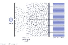
The first experimental evidence that atoms can absorb or emit e.m. energy was reported in 1859 by G Kirchhof and R Bunsen. It is possible to measure emission spectra, e.g. by recording the light emitted by a heated gas sample made of the same atoms and the absorption spectra by collimating a continuous light beam on a similar gas and detecting the transmitted signal. These experiments prove that: (i) the absorption/emission spectrum of any atom is specific to that atom, thus allowing unambiguous identification of any chemical species; (ii) both absorption and emission spectra consist in a series of discrete lines; (iii) absorption and emission lines of any given atom fall at the very same wavelengths.

In the specific case of hydrogen, spectral lines are found at wavelengths supplied by the phenomenological Rydberg equation
$$
\frac{1}{\lambda}=\mathcal{R}{\mathrm{H}}\left(\frac{1}{n_1^2}-\frac{1}{n_2^2}\right) $$ where $\mathcal{R}{\mathrm{H}}=109677 \mathrm{~cm}^{-1}$ is known as Rydberg constant. The $n_1$ and $n_2$ integer numbers identify the spectral series according to the following combination
$$
\begin{array}{lcc}
n_1=1 & \text { and } & n_2=2,3,4, \ldots \text { Lyman series } \
n_1=2 & \text { and } & n_2=3,4,5, \ldots \text { Balmer series } \
n_1=3 & \text { and } & n_2=4,5,6, \ldots \text { Paschen series } \
n_1=4 & \text { and } & n_2=5,6,7, \ldots \text { Brackett series } \
n_1=5 & \text { and } & n_2=6,7,8, \ldots \text { Pfund series }
\end{array}
$$
where each series is named after the scientist that first discovered it. Equation (1.16) holds for both absorbed or emitted light, consistently with experiments.

In order to allow the nuclear $\mathrm{H}$ atom to honour equation (1.16) we need to add some new hypotheses going beyond the unsuccessful classical model. They have been elaborated in 1913 by $\mathrm{N}$ Bohr who further exploited the new quantum approach pioneered by Planck and Einstein. The first step was to postulate that the electron could move only along those planar and circular orbits for which its angular momentum is an integer multiple of $\hbar=h / 2 \pi$. According to the first Bohr postulate, the modulus $l$ of the electron angular momentum is therefore given by ${ }^{13}$
$$
l=m_{\mathrm{e}} v r_n=n \hbar
$$
where $r_n$ is the radius of the orbit labelled by the integer number $n=1,2,3, \ldots$ and $v$ is the electron speed. The orbits allowed by equation (1.18) are named stationary states since Bohr further assumed that no emission of e.m. waves occurs when the electron is in such stable orbits.

物理代写|原子物理代写Atomic and Molecular Physics代考|The dual nature of physical phenomena

It is a matter of common experience that macroscopic physical phenomena reveal either as waves or as particles. By contrast, the Einstein hypothesis about the nature of e.m. waves as a flux of photons challenges this (pre)conception, which we now understand to be only due to the limits of our sensorial experience of the physical word. Light can in fact manifest either as a wave or as a beam of (pseudo)particles, according to the actual phenomenon we are addressing. Certainly the physics of our ocular vision or the propagation of light in vacuum are phenomena very well described by wave equations. On the other hand, the absorption/emission of light by an atomic system or the photoemission of electrons from a metal plate can only be explained by invoking the concept of photon.

In principle, we could speculate that this duality is similarly valid for massive particles, as first discussed by $\mathrm{L}$ de Broglie in 1924. If for a photon we can relate wave-like and particle-like properties through such relations as $E=h \nu$ or $\mathbf{p}=\hbar \mathbf{k}$ (where $\mathbf{p}$ is the photon momentum and $\mathbf{k}$ is the wavevector of the corresponding e.m. wave), then we could guess that a matter wave of wavelength $\lambda$ is associated with any particle with mass $m$ and moving with velocity $\mathbf{v}$ according to
$$
\lambda=\frac{h}{p}=\frac{h}{m v}=\frac{h}{2 m E_{\mathrm{kin}}}
$$
where $\mathbf{p}=m v$ is of course the particle momentum and $E_{\mathrm{kin}}=m v^2 / 2$ is its kinetic energy. This statement is nothing other than a speculation if no experimental evidence is supplied to support it.

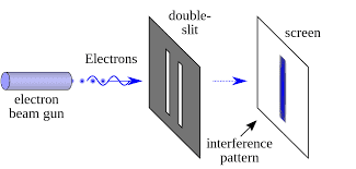
Interestingly enough, we have a convincing laboratory proof $[1,2,11]$ : a beam of electrons is diffracted by a crystalline sample giving rise to constructive/destructive interference phenomena as they were in fact waves. This experience, firstly performed by $\mathrm{C} \mathrm{L}$ Davisson and $\mathrm{L} \mathrm{H}$ Germer in 1926, provided a direct confirmation that the wavelength of diffracted electrons was exactly that predicted by de Broglie. So, electrons can be safely described as massive particles when studying electric phenomena (electrostatics or even the photoelectric effect), while they are better described as matter waves when diffracted by a crystal. Over the years, a large number of additional experiments proved that microscopic massive objects behave as waves (for instance, diffraction and interference have been observed in systems consisting of atom beams).

原子物理代考

物理代写|原子物理代写Atomic and Molecular Physics代考|Back to atomic spectra: the Bohr model

原子发射光谱的多重性和离散性已被引用两次，分别使汤姆森模型和卢瑟福模型的经典处理无效。值得更 详细地讨论主要的光谱实验结果，以解决我们遇到的问题。

G Kirchhof 和 R Bunsen 于 1859 年报告了原子可以吸收或发射 em 能量的第一个实验证据。可以测量发 射光谱，例如通过记录由相同原子制成的加热气体样品发射的光，以及通过将连续光束准直到类似气体上 并检测传输信号来测量吸收光谱。这些实验证明：(i) 任何原子的吸收/发射光谱都是特定于该原子的，因 此可以明确识别任何化学物质；(ii) 吸收光谱和发射光谱都由一系列离散的线组成；(iii) 任何给定原子的吸 收线和发射线都落在完全相同的波长处。
在氢的特定情况下，光谱线位于唯象里德堡方程 $\$ \$$
Ifrac ${1}{\backslash a m b d a}=I m a t h c a|{R}{\mid m a t h r m{H}}| l e f t\left(I f r a c{1)\right.$ 提供的波长处 $\left.\left.\left{n_{-} 1^{\wedge} 2\right}-\mid f r a c{1} n_{-} 2^{\wedge} 2\right} \mid r i g h t\right)$ $\$ \$$ 其中 $\$ 1$ mathcal{R} ${\backslash m a t h r m{\mathrm{H}}}=109677 \backslash$ mathrm ${\sim \mathrm{cm}} \wedge{-1}$
isknownasRydbergconstant.Then_1个andn_2
integernumbersidentifythespectralseriesaccordingtothe followingcombination
$n_1=1 \quad$ and $n_2=2,3,4, \ldots$ Lyman series $n_1=2 \quad$ and $n_2=3,4,5, \ldots$ Balmer series $\$$
其中每个系列都以第一个发现它的科学家的名字命名。方程式 (1.16) 对吸收光或发射光均成立，与实验一 致。
为了让核H为了尊重方程 (1.16)，我们需要添加一些超越不成功的经典模型的新假设。它们在 1913 年由 $\mathrm{N}$ 玻尔进一步开发了普朗克和爱因斯坦开创的新量子方法。第一步是假设电子只能沿着其角动量为整数倍 的平面和圆形轨道运动 $\hbar=h / 2 \pi$. 根据第一玻尔假设，模数l因此，电子角动量由下式给出 ${ }^{13}$
$$
l=m_{\mathrm{e}} v r_n=n \hbar
$$
在哪里 $r_n$ 是由整数标记的轨道的半径 $n=1,2,3, \ldots$ 和 $v$ 是电子速度。等式 (1.18) 允许的轨道被命名为静 止状态，因为玻尔进一步假设当电子处于这种稳定轨道时不会发生 em 波的发射。

物理代写|原子物理代写Atomic and Molecular Physics代考|The dual nature of physical phenomena

宏观物理现象要么表现为波，要么表现为粒子，这是一个普遍的经验问题。相比之下，爱因斯坦关于 em 波作为光子通量的性质的假设挑战了这个（预）概念，我们现在理解这只是由于我们对物理词的感官体验 的限制。根据我们正在处理的实际现象，光实际上可以表现为波或（伪）粒子束。当然，我们肉眼视觉的 物理学或光在真空中的传播都是用波动方程很好地描述的现象。另一方面，原子系统对光的吸收/发射或 金属板对电子的光电发射只能通过光子的概念来解释。
原则上，我们可以推测这种对偶性同样适用于大质量粒子，正如首先由L德布罗意 (de Broglie) 于 1924 年发表。如果对于光子，我们可以通过以下关系将波状和粒子状特性联系起来 $E=h \nu$ 或者 $\mathbf{p}=\hbar \mathbf{k}$ （在 哪里 $\mathbf{p}$ 是光子动量和 $\mathbf{k}$ 是对应的em波的波矢），则可以推测波长为 $\lambda$ 与任何有质量的粒子相关联 $m$ 并以速 度移动 $\mathbf{v}$ 根据
$$
\lambda=\frac{h}{p}=\frac{h}{m v}=\frac{h}{2 m E_{\mathrm{kin}}}
$$
在哪里 $\mathbf{p}=m v$ 当然是粒子动量和 $E_{\mathrm{kin}}=m v^2 / 2$ 是它的动能。如果没有提供实验证据支持，这种说法 只不过是一种推测。
有趣的是，我们有令人信服的实验室证明 $[1,2,11]$ ：电子束被晶体样品衍射，产生建设性/破坏性干涉现 象，因为它们实际上是波。此次体验，首先由CL戴维森和LHGermer 在 1926 年直接证实了衍射电子的 波长与德布罗意所预测的完全一致。因此，在研究电现象（静电学甚至光电效应) 时，电子可以安全地描 述为大质量粒子，而当它们被晶体衍射时，则更好地描述为物质波。多年来，大量额外的实验证明微观大 质量物体表现为波 (例如，在由原子束组成的系统中观察到衍射和干涉)。

统计代写请认准statistics-lab™. statistics-lab™为您的留学生涯保驾护航。

金融工程代写

金融工程是使用数学技术来解决金融问题。金融工程使用计算机科学、统计学、经济学和应用数学领域的工具和知识来解决当前的金融问题，以及设计新的和创新的金融产品。

非参数统计代写

非参数统计指的是一种统计方法，其中不假设数据来自于由少数参数决定的规定模型；这种模型的例子包括正态分布模型和线性回归模型。

广义线性模型代考

广义线性模型（GLM）归属统计学领域，是一种应用灵活的线性回归模型。该模型允许因变量的偏差分布有除了正态分布之外的其它分布。

术语 广义线性模型（GLM）通常是指给定连续和/或分类预测因素的连续响应变量的常规线性回归模型。它包括多元线性回归，以及方差分析和方差分析（仅含固定效应）。

有限元方法代写

有限元方法（FEM）是一种流行的方法，用于数值解决工程和数学建模中出现的微分方程。典型的问题领域包括结构分析、传热、流体流动、质量运输和电磁势等传统领域。

有限元是一种通用的数值方法，用于解决两个或三个空间变量的偏微分方程（即一些边界值问题）。为了解决一个问题，有限元将一个大系统细分为更小、更简单的部分，称为有限元。这是通过在空间维度上的特定空间离散化来实现的，它是通过构建对象的网格来实现的：用于求解的数值域，它有有限数量的点。边界值问题的有限元方法表述最终导致一个代数方程组。该方法在域上对未知函数进行逼近。[1] 然后将模拟这些有限元的简单方程组合成一个更大的方程系统，以模拟整个问题。然后，有限元通过变化微积分使相关的误差函数最小化来逼近一个解决方案。

tatistics-lab作为专业的留学生服务机构，多年来已为美国、英国、加拿大、澳洲等留学热门地的学生提供专业的学术服务，包括但不限于Essay代写，Assignment代写，Dissertation代写，Report代写，小组作业代写，Proposal代写，Paper代写，Presentation代写，计算机作业代写，论文修改和润色，网课代做，exam代考等等。写作范围涵盖高中，本科，研究生等海外留学全阶段，辐射金融，经济学，会计学，审计学，管理学等全球99%专业科目。写作团队既有专业英语母语作者，也有海外名校硕博留学生，每位写作老师都拥有过硬的语言能力，专业的学科背景和学术写作经验。我们承诺100%原创，100%专业，100%准时，100%满意。

随机分析代写

随机微积分是数学的一个分支，对随机过程进行操作。它允许为随机过程的积分定义一个关于随机过程的一致的积分理论。这个领域是由日本数学家伊藤清在第二次世界大战期间创建并开始的。

时间序列分析代写

随机过程，是依赖于参数的一组随机变量的全体，参数通常是时间。 随机变量是随机现象的数量表现，其时间序列是一组按照时间发生先后顺序进行排列的数据点序列。通常一组时间序列的时间间隔为一恒定值（如1秒，5分钟，12小时，7天，1年），因此时间序列可以作为离散时间数据进行分析处理。研究时间序列数据的意义在于现实中，往往需要研究某个事物其随时间发展变化的规律。这就需要通过研究该事物过去发展的历史记录，以得到其自身发展的规律。

回归分析代写

多元回归分析渐进（Multiple Regression Analysis Asymptotics）属于计量经济学领域，主要是一种数学上的统计分析方法，可以分析复杂情况下各影响因素的数学关系，在自然科学、社会和经济学等多个领域内应用广泛。

MATLAB代写

MATLAB 是一种用于技术计算的高性能语言。它将计算、可视化和编程集成在一个易于使用的环境中，其中问题和解决方案以熟悉的数学符号表示。典型用途包括：数学和计算算法开发建模、仿真和原型制作数据分析、探索和可视化科学和工程图形应用程序开发，包括图形用户界面构建MATLAB 是一个交互式系统，其基本数据元素是一个不需要维度的数组。这使您可以解决许多技术计算问题，尤其是那些具有矩阵和向量公式的问题，而只需用 C 或 Fortran 等标量非交互式语言编写程序所需的时间的一小部分。MATLAB 名称代表矩阵实验室。MATLAB 最初的编写目的是提供对由 LINPACK 和 EISPACK 项目开发的矩阵软件的轻松访问，这两个项目共同代表了矩阵计算软件的最新技术。MATLAB 经过多年的发展，得到了许多用户的投入。在大学环境中，它是数学、工程和科学入门和高级课程的标准教学工具。在工业领域，MATLAB 是高效研究、开发和分析的首选工具。MATLAB 具有一系列称为工具箱的特定于应用程序的解决方案。对于大多数 MATLAB 用户来说非常重要，工具箱允许您学习和应用专业技术。工具箱是 MATLAB 函数（M 文件）的综合集合，可扩展 MATLAB 环境以解决特定类别的问题。可用工具箱的领域包括信号处理、控制系统、神经网络、模糊逻辑、小波、仿真等。

R语言代写	问卷设计与分析代写
PYTHON代写	回归分析与线性模型代写
MATLAB代写	方差分析与试验设计代写
STATA代写	机器学习/统计学习代写
SPSS代写	计量经济学代写
EVIEWS代写	时间序列分析代写
EXCEL代写	深度学习代写
SQL代写	各种数据建模与可视化代写

如果你也在 怎样代写原子物理Atomic and Molecular Physics这个学科遇到相关的难题，请随时右上角联系我们的24/7代写客服。

原子物理学是AMO的子领域，研究原子作为电子和原子核的孤立系统，而分子物理学是研究分子的物理特性。

statistics-lab™ 为您的留学生涯保驾护航 在代写原子物理Atomic and Molecular Physics方面已经树立了自己的口碑, 保证靠谱, 高质且原创的统计Statistics代写服务。我们的专家在代写原子物理Atomic and Molecular Physics代写方面经验极为丰富，各种代写原子物理Atomic and Molecular Physics相关的作业也就用不着说。

我们提供的原子物理Atomic and Molecular Physics及其相关学科的代写，服务范围广, 其中包括但不限于:

• Statistical Inference 统计推断
• Statistical Computing 统计计算
• Advanced Probability Theory 高等概率论
• Advanced Mathematical Statistics 高等数理统计学
• (Generalized) Linear Models 广义线性模型
• Statistical Machine Learning 统计机器学习
• Longitudinal Data Analysis 纵向数据分析
• Foundations of Data Science 数据科学基础

物理代写|原子物理代写Atomic and Molecular Physics代考|The quantum nature of physical laws

The above achievements about the structure of matter clearly bring out the next objective, namely: understanding the inner physics of an interacting planetary system made by one or more electron(s) and a nucleus.

Let us consider the hydrogen atom and assume that for its ground state the radius of the circular electronic orbit is $a_0=0.529 \AA$, hereafter referred to as Bohr radius ${ }^8$. In this classical model, the electron is rotating at speed
$$
v_0=\sqrt{\frac{e^2}{4 \pi \varepsilon_0 m_{\mathrm{e}} a_0}} \sim 2 \times 10^6 \mathrm{~m} \mathrm{~s}^{-1}
$$
feeling a linear acceleration
$$
a=\frac{v_0^2}{a_0} \sim 9 \times 10^{22} \mathrm{~m} \mathrm{~s}^{-2}
$$
since it moves under the action of the Coulomb central field generated by the nucleus. Now, classical physics dictates [8] that any accelerated particle of charge $\pm e$ irradiates electromagnetic energy at power
$$
P=\frac{e^2 a^2}{6 \pi \varepsilon_0 c^3}
$$
where $c$ is the speed of light. In the atomic case we are discussing, this corresponds to $P_H \sim 4 \times 10^{11} \mathrm{eV} \mathrm{s}^{-1}$ representing the emission power of hydrogen ${ }^9$. Chemistry provides evidence that the ionisation energy of the $\mathrm{H}$ atom in its ground state is $13.6 \mathrm{eV}$, that we can consider as the net amount of energy stored in a bound electron-proton planetary system. Since such an energy is dissipated by irradiation at the rate $P_{\mathrm{H}}$, we immediately obtain that a hydrogen atom would lose all its energy in about $10^{-11} \mathrm{~s}$. Over such an astonishingly short lapse of time the electron speed would vanish, likewise the orbital radius: the electron ‘falls’ on the nucleus. By generalising this result we come to a rather disturbing conclusion, namely: according to classical physics matter should not be stable or, equivalently, we should not observe the Universe in its present appearance. Bad enough, this discouraging result is not the only failure of the classical planetary atomic model: the trajectory of the electron falling motion is predicted to be a spiral whose radius continuously varies as $r(t)=a_0-\mathcal{A} t^{1 / 3}$, where $\mathcal{A}$ is a suitable constant. This in turn implies that the emission spectrum of the hydrogen atom should be continuous, completely at odds with experimental evidence as already commented on in section 1.1.3.

The conclusion we can draw is unequivocal: the Rutherford model cannot be adopted in bundle with the laws of classical physics. Since such a model has proved to be very successful in describing $\alpha$ particle scattering, it is really hard to discard it: in fact, this was not the option chosen by scientists working in this field. Rather, some new physics is needed which must be inherently non-classical.

物理代写|原子物理代写Atomic and Molecular Physics代考|A necessary digression

In search for some non-classical concepts possibly useful to our advancement, we will briefly discuss the physics of blackbody radiation and the photoelectric effect. A more extensive treatment of both phenomena falls beyond the scope of this book and can be found elsewhere $[2,11]$. The emerging new concepts will be then applied to the interpretation of the atomic spectra in the next section.

It is known that any solid body can both absorb and emit light. These phenomena are typically described by the spectral absorption $a_\nu$ or spectral emission $e_\nu$, respectively defined as the e.m. power absorbed or emitted by the unit of surface area of the body at frequency $\nu$. While $a_\nu$ and $e_\nu$ individually depend on the actual physico-chemical properties of the solid and the morphological features of its surface, their ratio is given, at any frequency, by a universal function of the sole temperature $T$, as first discussed by G Kirchhoff in 1859-62. A blackbody is an ideal system characterised by $a_\nu=1$. In practice, it can be mimicked by a solid sample containing a cavity with blackened inner surfaces and a small hole through which e.m. radiation can be exchanged with the surrounding ambient: once a radiation penetrates into the cavity, it is very unlikely to be able to escape (absorption close to $100 \%$ ) because of the small size of the orifice; on the other hand, thermal radiation can be emitted through the very same aperture (blackbody radiation).

By bringing such a system to an equilibrium temperature $T$, it is possible to record its emission spectrum, customarily addressed as the blackbody radiation: it is a nonmonotonic function of the e.m. frequency, which also depends on temperature. The experimental findings are summarised by two laws, respectively: (i) in 1879 J Stefan derived that the total e.m. power $P_{\text {tot }}(T)$ emitted by the unit of surface area is given by
$$
P_{\mathrm{tot}}(T)=\sigma_{\mathrm{S}} T^4
$$
where $\sigma_{\mathrm{S}}=5.67 \times 10^{-8} \mathrm{~W} \mathrm{~m}^{-2} \mathrm{~K}^{-4}$ is nowadays known as Stefan constant; (ii) in $1893 \mathrm{~W}$ Wien proved that if $\nu_{\max }$ is defined as the frequency at which we observe the maximum emission intensity, then it holds
$$
\frac{\nu_{\max }}{T}=\text { constant }
$$ a result which is usually referred to as the Wien displacement law.

原子物理代考

物理代写|原子物理代写Atomic and Molecular Physics代考|The quantum nature of physical laws

上述关于物质结构的成就清楚地提出了下一个目标，即：了解由一个或多个电子和原子核构成的相互作用 行星系统的内部物理。
让我们考虑氢原子并假设其基态的圆形电子轨道半径为 $a_0=0.529 \backslash \mathrm{AA}$ ， 以下简称玻尔半径 ${ }^8$. 在这个经 典模型中，电子高速旋转
$$
v_0=\sqrt{\frac{e^2}{4 \pi \varepsilon_0 m_{\mathrm{e}} a_0}} \sim 2 \times 10^6 \mathrm{~m} \mathrm{~s}^{-1}
$$
感觉线性加速
$$
a=\frac{v_0^2}{a_0} \sim 9 \times 10^{22} \mathrm{~m} \mathrm{~s}^{-2}
$$
因为它在原子核产生的库仑中心场的作用下运动。现在，经典物理学规定 [8] 任何加速的电荷粒子 $\pm e$ 在功 率辐射电磁能
$$
P=\frac{e^2 a^2}{6 \pi \varepsilon_0 c^3}
$$
在哪里 $c$ 是光速。在我们讨论的原子情况下，这对应于 $P_H \sim 4 \times 10^{11} \mathrm{eVs}^{-1}$ 代表氢气的发射功率 ${ }^9$. 化 学提供的证据表明，H处于基态的原子是 $13.6 \mathrm{eV}$ ，我们可以将其视为束缚电子 – 质子行星系统中存储的 净能量。由于这样的能量通过辐射以以下速率耗散 $P_{\mathrm{H}}$ ，我们立即得到一个氢原子会在大约 $10^{-11} \mathrm{~s}$. 在如 此短得惊人的时间流逝后，电子速度将消失，轨道半径也将消失：电子”落”在原子核上。通过概括这个结 果，我们得出了一个相当令人不安的结论，即：根据经典物理学，物质不应该是稳定的，或者说，我们不 应该观察宇宙目前的样子。糟糕的是，这个令人沮丧的结果并不是经典行星原子模型的唯一失败：电子下 落运动的轨迹被预测为螺旋形，其半径连续变化为 $r(t)=a_0-\mathcal{A} t^{1 / 3}$ ，在哪里 $\mathcal{A}$ 是一个合适的常数。 这反过来意味着氢原子的发射光谱应该是连续的，这与 1.1.3 节中已经评论过的实验证据完全不一致。
我们可以得出的结论是明确的：卢瑟福模型不能与经典物理定律捆绑在一起采用。由于这样的模型已被证 明非常成功地描述了 $\alpha$ 粒子散射，真的很难丟弃它：事实上，这不是从事该领域工作的科学家选择的选 项。相反，需要一些本质上必须是非经典的新物理学。

物理代写|原子物理代写Atomic and Molecular Physics代考|A necessary digression

为了寻找一些可能对我们的进步有用的非经典概念，我们将简要讨论黑体辐射和光电效应的物理学。对这 两种现象的更广泛的处理超出了本书的范围，可以在别处找到 $[2,11]$. 新兴的新概念将在下一节中应用于 解释原子光谱。
众所周知，任何固体都可以吸收和发射光。这些现象通常用光谱吸收来描述 $a_\nu$ 或光谱发射 $e_\nu$ ，分别定义 为身体表面积单位在频率下吸收或发射的电磁功率 $\nu$. 尽管 $a_\nu$ 和 $e_\nu$ 分别取决于固体的实际物理化学性质及 其表面的形态特征，它们的比率在任何频率下由唯一温度的通用函数给出 $T$ ，正如 G Kirchhoff 在 185962 年首次讨论的那样。黑体是一个理想的系统，其特征是 $a_\nu=1$. 在实践中，它可以通过一个固体样品 来模拟，该样品包含一个内表面发黑的空腔和一个小孔，通过该小孔可以与周围环境交换电磁辐射：一旦 辐射穿透空腔，就不太可能逃逸（吸收接近 $100 \%$ ) 因为孔口尺寸小；另一方面，热辐射可以通过完全相 同的孔径 (黑体辐射) 发射。
通过使这样的系统达到平衡温度 $T$ ，可以记录其发射光谱，通常称为黑体辐射：它是 em 频率的非单调函 数，它也取决于温度。实验结果分别由两个定律总结：(i) 1879 年J Stefan 推导出总 em 功率 $P_{\text {tot }}(T)$ 由 表面积单位发出的由下式给出
$$
P_{\text {tot }}(T)=\sigma_{\mathrm{S}} T^4
$$
在哪里 $\sigma_{\mathrm{S}}=5.67 \times 10^{-8} \mathrm{~W} \mathrm{~m}^{-2} \mathrm{~K}^{-4}$ 现在被称为 Stefan 常数； (ii) 在 $1893 \mathrm{~W}$ 维恩证明如果 $\nu_{\text {max }}$ 被 定义为我们观察到最大发射强度的频率，那么它成立
$$
\frac{\nu_{\max }}{T}=\text { constant }
$$
通常称为维恩位移定律的结果。

统计代写请认准statistics-lab™. statistics-lab™为您的留学生涯保驾护航。

金融工程代写

金融工程是使用数学技术来解决金融问题。金融工程使用计算机科学、统计学、经济学和应用数学领域的工具和知识来解决当前的金融问题，以及设计新的和创新的金融产品。

非参数统计代写

非参数统计指的是一种统计方法，其中不假设数据来自于由少数参数决定的规定模型；这种模型的例子包括正态分布模型和线性回归模型。

广义线性模型代考

广义线性模型（GLM）归属统计学领域，是一种应用灵活的线性回归模型。该模型允许因变量的偏差分布有除了正态分布之外的其它分布。

术语 广义线性模型（GLM）通常是指给定连续和/或分类预测因素的连续响应变量的常规线性回归模型。它包括多元线性回归，以及方差分析和方差分析（仅含固定效应）。

有限元方法代写

有限元方法（FEM）是一种流行的方法，用于数值解决工程和数学建模中出现的微分方程。典型的问题领域包括结构分析、传热、流体流动、质量运输和电磁势等传统领域。

有限元是一种通用的数值方法，用于解决两个或三个空间变量的偏微分方程（即一些边界值问题）。为了解决一个问题，有限元将一个大系统细分为更小、更简单的部分，称为有限元。这是通过在空间维度上的特定空间离散化来实现的，它是通过构建对象的网格来实现的：用于求解的数值域，它有有限数量的点。边界值问题的有限元方法表述最终导致一个代数方程组。该方法在域上对未知函数进行逼近。[1] 然后将模拟这些有限元的简单方程组合成一个更大的方程系统，以模拟整个问题。然后，有限元通过变化微积分使相关的误差函数最小化来逼近一个解决方案。

tatistics-lab作为专业的留学生服务机构，多年来已为美国、英国、加拿大、澳洲等留学热门地的学生提供专业的学术服务，包括但不限于Essay代写，Assignment代写，Dissertation代写，Report代写，小组作业代写，Proposal代写，Paper代写，Presentation代写，计算机作业代写，论文修改和润色，网课代做，exam代考等等。写作范围涵盖高中，本科，研究生等海外留学全阶段，辐射金融，经济学，会计学，审计学，管理学等全球99%专业科目。写作团队既有专业英语母语作者，也有海外名校硕博留学生，每位写作老师都拥有过硬的语言能力，专业的学科背景和学术写作经验。我们承诺100%原创，100%专业，100%准时，100%满意。

随机分析代写

随机微积分是数学的一个分支，对随机过程进行操作。它允许为随机过程的积分定义一个关于随机过程的一致的积分理论。这个领域是由日本数学家伊藤清在第二次世界大战期间创建并开始的。

时间序列分析代写

随机过程，是依赖于参数的一组随机变量的全体，参数通常是时间。 随机变量是随机现象的数量表现，其时间序列是一组按照时间发生先后顺序进行排列的数据点序列。通常一组时间序列的时间间隔为一恒定值（如1秒，5分钟，12小时，7天，1年），因此时间序列可以作为离散时间数据进行分析处理。研究时间序列数据的意义在于现实中，往往需要研究某个事物其随时间发展变化的规律。这就需要通过研究该事物过去发展的历史记录，以得到其自身发展的规律。

回归分析代写

多元回归分析渐进（Multiple Regression Analysis Asymptotics）属于计量经济学领域，主要是一种数学上的统计分析方法，可以分析复杂情况下各影响因素的数学关系，在自然科学、社会和经济学等多个领域内应用广泛。

MATLAB代写

MATLAB 是一种用于技术计算的高性能语言。它将计算、可视化和编程集成在一个易于使用的环境中，其中问题和解决方案以熟悉的数学符号表示。典型用途包括：数学和计算算法开发建模、仿真和原型制作数据分析、探索和可视化科学和工程图形应用程序开发，包括图形用户界面构建MATLAB 是一个交互式系统，其基本数据元素是一个不需要维度的数组。这使您可以解决许多技术计算问题，尤其是那些具有矩阵和向量公式的问题，而只需用 C 或 Fortran 等标量非交互式语言编写程序所需的时间的一小部分。MATLAB 名称代表矩阵实验室。MATLAB 最初的编写目的是提供对由 LINPACK 和 EISPACK 项目开发的矩阵软件的轻松访问，这两个项目共同代表了矩阵计算软件的最新技术。MATLAB 经过多年的发展，得到了许多用户的投入。在大学环境中，它是数学、工程和科学入门和高级课程的标准教学工具。在工业领域，MATLAB 是高效研究、开发和分析的首选工具。MATLAB 具有一系列称为工具箱的特定于应用程序的解决方案。对于大多数 MATLAB 用户来说非常重要，工具箱允许您学习和应用专业技术。工具箱是 MATLAB 函数（M 文件）的综合集合，可扩展 MATLAB 环境以解决特定类别的问题。可用工具箱的领域包括信号处理、控制系统、神经网络、模糊逻辑、小波、仿真等。

R语言代写	问卷设计与分析代写
PYTHON代写	回归分析与线性模型代写
MATLAB代写	方差分析与试验设计代写
STATA代写	机器学习/统计学习代写
SPSS代写	计量经济学代写
EVIEWS代写	时间序列分析代写
EXCEL代写	深度学习代写
SQL代写	各种数据建模与可视化代写

如果你也在 怎样代写原子物理Atomic and Molecular Physics这个学科遇到相关的难题，请随时右上角联系我们的24/7代写客服。

原子物理学是AMO的子领域，研究原子作为电子和原子核的孤立系统，而分子物理学是研究分子的物理特性。

statistics-lab™ 为您的留学生涯保驾护航 在代写原子物理Atomic and Molecular Physics方面已经树立了自己的口碑, 保证靠谱, 高质且原创的统计Statistics代写服务。我们的专家在代写原子物理Atomic and Molecular Physics代写方面经验极为丰富，各种代写原子物理Atomic and Molecular Physics相关的作业也就用不着说。

我们提供的原子物理Atomic and Molecular Physics及其相关学科的代写，服务范围广, 其中包括但不限于:

• Statistical Inference 统计推断
• Statistical Computing 统计计算
• Advanced Probability Theory 高等概率论
• Advanced Mathematical Statistics 高等数理统计学
• (Generalized) Linear Models 广义线性模型
• Statistical Machine Learning 统计机器学习
• Longitudinal Data Analysis 纵向数据分析
• Foundations of Data Science 数据科学基础

物理代写|原子物理代写Atomic and Molecular Physics代考|The atomistic structure of matter

Matter offers to our senses as a continuum, categorised as a solid, liquid or gas by simply observing whether it has, respectively, a definite volume and shape, or just a definite volume, or none of them. According to this continuum picture, we can split (in the case of solids) or separate (in the case of liquids and gases) any given matter sample into two (or more) parts and, in principle, we can repeat this operation an arbitrary number of times, still obtaining continuum matter specimens (eventually very small).

This macroscopic description is contrasted by a more accurate observation of the structure of matter, as first elaborated at the dawn of the nineteenth century through the combined efforts of a number of scientists ${ }^1$. On the basis of chemical evidence, it was observed that matter can be formed either by pure substances (or elements) and by compounds mixing two or more elements. Next, a law of multiple definite proportions for any compound was formulated: the fixed amount of a given element and the corresponding amounts of any other element needed to form a compound are in the ratio of small integer numbers. For instance: for any given ‘quantity’ of, say, hydrogen there are needed two ‘quantities’ of oxygen to form that compound we name water. These empirical observations suggest that matter in fact cannot be arbitrarily divided into increasingly smaller parts, still maintaining its original chemical properties. Rather, a new picture was emerging: matter in whatever state of aggregation is made by elements or compounds; each element is made by elementary constituents, hereafter referred to as atoms; and compounds are formed by combining numbers of different atoms in simple ratios. It was a natural guess assuming that atoms of the same element are identical in nature and have just the same weight. Since the atomistic structure of matter cannot be addressed by our senses, it was further assumed that atoms are really very small.

Once that the concept of the atom is accepted, we can elaborate a picture of matter rather different than the continuum one, namely: any solid of fluid substance is formed either by an assembly of atoms of just one kind or by an assembly of molecules. These latter material entities are the smallest parts of any compound substance that determine its chemical properties. It is then straightforward to introduce the concept of mole as the most natural unit for quantifying the actual amount of matter forming a given specimen: a mole is that quantity weighting in grams the same number expressing the atomic or molecular weight ${ }^2$. Based on thermodynamical arguments, Avogadro argued that a mole of any substance contains the very same number $\mathcal{N}{\mathrm{A}}$ of atoms or molecules, whether the substance is respectively elemental or compound. Such a number was determined by several different experimental methods [2] based on thermodynamical, electrochemical, or $\mathrm{x}$-ray diffraction measurements; its more accurate value is $$ \mathcal{N}{\mathrm{A}}=6.0221415 \times 10^{23} \mathrm{~mole}^{-1}
$$
which allows for a qualitative estimation of the typical size of an atom. By assuming that a solid matter sample with uniform mass density $\rho$ is made by close-packed spherical atoms ${ }^3$ with diameter $d$, we simply obtain an order-of-magnitude estimation of the typical atom size: $d \sim 1-2 \times 10^{-10} \mathrm{~m}$.

物理代写|原子物理代写Atomic and Molecular Physics代考|What are atoms made of?

None of the experimental evidence discussed in the previous section provides information about the inner structure of an atom, nor do the phenomenological theories based on the early atomistic hypothesis indeed require any knowledge about this issue (for instance, the kinetic theory of gases assumes structureless atoms).
There is, however, direct and indirect evidence that matter-made of atomsdoes contain electrically charged particles. To name just a few examples: (i) by applying an electric field to a polar liquid, an electrolytic current is observed and explained, as originally proposed by M Faraday, in terms of dissociation of molecules into positive and negative constituents, hereafter referred to as ions, drifting in opposite directions; (ii) particles like $\alpha$ or $\beta$ ones (which we nowadays recognise as helium nuclei and electrons, respectively) emitted by radioactive substances are differently deflected by an external magnetic field due to the Lorentz force, thus proving that they carry a charge; (iii) an electrical current is observed in metals under bias, as proved by electrical measurements. We must eventually conclude not only that is matter made from atoms, but also that atoms are made by substructures with either positive or negative electric charge. The differently charged constituents of atoms have different masses as well.

Chemistry as a whole supplies evidence ${ }^6$ that the negative substructures are electrons, i.e. particles carrying just one elementary electric charge $e=1.60219 \times 10^{-19} \mathrm{C}$ with a mass $m_{\mathrm{e}}=9.10953 \times 10^{-31} \mathrm{~kg}=5.4858 \times 10^{-4}$ a.m.u. An accurate estimation of the $e / m_{\mathrm{e}}$ ratio was for the first time provided by the suspended oil droplet experiment performed by R A Millikan in 1909-10, while the concept that the electric charge was not infinitely divisible was previously elaborated by M Faraday in 1883 when he worked out the fundamental law of electrolysis in the form
$$
M=\frac{1}{F} \frac{w}{\zeta} Q
$$
stating that the mass $M$ of a substance liberated at an electrode over a given time is always proportional to the net charge $Q$ passed through the electrolytic solution in the same time. In equation (1.2) $\zeta$ is the valence of the atoms of the liberated substance, while $F=9.648646 \times 10^4 \mathrm{C} / \mathrm{mole}$ is the so-called Faraday constant. Since a charge $Q=964864.6 \mathrm{C}$ liberates exactly 1 mole of a monovalent $(\zeta=1)$ substance, the elementary electric charge is naturally defined as $e=F / \mathcal{N}_{\mathrm{A}}$, which provides the value of the electron charge reported above. The true existence of electrons is confirmed in many ways [2], including: the photoelectric effect (i.e. the emission of electrons by a metal surface illuminated by ultraviolet radiation), the deflection of cathode rays by a magnetic field or, finally, the thermionic emission phenomenon (i.e. the emission of electrons from solids heated to a suitably high temperature).

Since atoms in their normal state are electrically neutral (likewise condensed matter), we must conclude that each atom is an electrically complex system, containing an equal amount of negative and positive charge. While the former is provided by a given number of electrons, the latter is in a still unknown form. In brief: if an atom contains $Z$ electrons, it must also contain other constituents with a total positive charge $+Z e$. The number $Z$ is known as atomic number. A further observation consists in comparing $m_{\mathrm{e}}$ to the mass $m_{\mathrm{H}}$ of the lightest atom, namely hydrogen $(\mathrm{H})$, containing just one electron: it results $m_{\mathrm{H}} \gg m$, thus implying that most of the atomic mass must be associated with the positively charged constituents.

原子物理代考

物理代写|原子物理代写Atomic and Molecular Physics代考|The atomistic structure of matter

物质以连续体的形式提供给我们的感官，通过简单地观察它是否分别具有确定的体积和形状，或者只是确 定的体积，或者没有它们，将其分类为固体、液体或气体。根据这张连续谱图，我们可以将任何给定的物 质样本 (在固体的情况下) 或分离（在液体和气体的情况下) 分成两个（或更多) 部分，原则上，我们可 以任意重复此操作多次，仍然获得连续物质标本（最终非常小）。
这种宏观描述与对物质结构的更准确观察形成对比，正如十九世纪初通过许多科学家的共同努力首次阐述 的那样 ${ }^1$. 根据化学证据，人们观察到物质可以由纯物质 (或元素) 形成，也可以由混合两种或多种元素的 化合物形成。接下来，制定了任何化合物的多重定比定律：给定元素的固定量与形成化合物所需的任何其 他元素的相应量是小整数之比。例如：对于任何给定“量”的氢气，都需要两个“量”的氧来形成我们命名为 水的化合物。这些经验观察表明，物质实际上不能被任意分成越来越小的部分，仍然保持其原有的化学性 质。相反，一种新的图景正在出现：无论元素或化合物处于何种聚合状态的物质；每个元素都是由基本成 分构成的，以下称为原子；化合物是通过以简单的比例组合多个不同原子而形成的。这是一个自然的猜 测，假设相同元素的原子在性质上是相同的并且具有相同的重量。由于我们的感官无法解决物质的原子结 构，因此进一步假设原子确实非常小。
一旦接受了原子的概念，我们就可以描绘出一种与连续体截然不同的物质图景，即：任何固体或流体物质 要么由仅一种原子的集合形成，要么由分子集合形成。后面这些物质实体是决定其化学性质的任何复合物 质的最小部分。然后直接引入摩尔的概念作为量化形成给定样本的物质的实际量的最自然单位：摩尔是以 克为单位的重量与表示原子量或分子量的相同数字 ${ }^2$. 基于热力学论证，阿伏加德罗认为任何物质的一摩尔 都包含完全相同的数字 $\mathcal{N}$ 原子或分子的物质，无论物质分别是元素还是化合物。这个数字是通过几种不 同的实验方法 [2] 基于热力学、电化学或x-射线衍射测量；它更准确的值是
$$
\mathcal{N A}=6.0221415 \times 10^{23} \mathrm{~mole}^{-1}
$$
这允许对原子的典型大小进行定性估计。通过假设具有均匀质量密度的固体物质样品 $\rho$ 由紧密堆积的球形 原子构成 ${ }^3$ 直径 $d$ ，我们简单地获得典型原子大小的数量级估计： $d \sim 1-2 \times 10^{-10} \mathrm{~m}$.

物理代写|原子物理代写Atomic and Molecular Physics代考|What are atoms made of?

上一节中讨论的实验证据都没有提供有关原子内部结构的信息，基于早期原子假设的唯象理论也确实不需 要任何关于这个问题的知识 (例如，气体动力学理论假设无结构原子).
然而，有直接和间接的证据表明，由原子构成的物质确实包含带电粒子。仅举几个例子：（i）通过对极性 液体施加电场，观察并解释了电解电流，正如 M Faraday 最初提出的那样，根据分子离解成正负成分，
以下称为作为离子，向相反的方向漂移；(ii) 颗粒如 $\alpha$ 或者 $\beta$ 放射性物质发射的电子 (我们现在分别称为氦 核和电子) 由于洛伦兹力而被外部磁场不同地偏转，从而证明它们带有电荷；(iii) 电流在金属中观察到偏 压，正如电气测量所证明的那样。我们最终必须得出结论，不仅物质是由原子构成的，而且原子是由带有 正电荷或负电荷的子结构构成的。原子的不同电荷成分也有不同的质量。
化学作为一个整体提供了证据 ${ }^6$ 负子结构是电子，即只携带一个基本电荷的粒子 $e=1.60219 \times 10^{-19} \mathrm{C}$ 有质量 $m_{\mathrm{e}}=9.10953 \times 10^{-31} \mathrm{~kg}=5.4858 \times 10^{-4}$ amu 的准确估计 $/ / m_{\mathrm{e}}$ RA Millikan 在 1909-10 年进行的悬浮油滴实验首次提供了比值，而电荷不可无限分割的概念则由 M Faraday 在 1883 年提出电解 基本定律时阐述在形式
$$
M=\frac{1}{F} \frac{w}{\zeta} Q
$$
说明质量 $M$ 在给定时间内在电极处释放的物质的量始终与净电荷成正比 $Q$ 同时通过电解液。在等式
(1.2）中 $\zeta$ 是释放物质原子的化合价，而 $F=9.648646 \times 10^4 \mathrm{C} / \mathrm{mole}$ 是所谓的法拉第常数。自收费 $Q=964864.6 \mathrm{C}$ 正好释放出 1 摩尔的单价化合物 $(\zeta=1)$ 物质，基本电荷自然定义为 $e=F / \mathcal{N}{\mathrm{A}}$ ，它 提供了上面报告的电子电荷值。电子的真实存在以多种方式得到证实 [2]，包括：光电效应（即被紫外线 辐射照射的金属表面发射电子）、阴极射线被磁场偏转，或者最后，热电子效应发射现象（即从加热到适 当高温的固体发射电子)。 由于处于正常状态的原子是电中性的（凝聚态物质也是如此），我们必须得出结论，每个原子都是一个电 复杂系统，包含等量的负电荷和正电荷。前者是由给定数量的电子提供的，而后者的形式仍然末知。简而 言之：如果一个原子包含 $Z$ 电子，它还必须包含具有总正电荷的其他成分 $+Z e$. 号码 $Z$ 被称为原子序数。 进一步的观察包括比较 $m{\mathrm{e}}$ 大众 $m_{\mathrm{H}}$ 最轻的原子，即氢 $(\mathrm{H})$ ，只包含一个电子：结果 $m_{\mathrm{H}} \gg m$ ，因此意味 着大部分原子质量必须与带正电的成分相关联。

统计代写请认准statistics-lab™. statistics-lab™为您的留学生涯保驾护航。

金融工程代写

金融工程是使用数学技术来解决金融问题。金融工程使用计算机科学、统计学、经济学和应用数学领域的工具和知识来解决当前的金融问题，以及设计新的和创新的金融产品。

非参数统计代写

非参数统计指的是一种统计方法，其中不假设数据来自于由少数参数决定的规定模型；这种模型的例子包括正态分布模型和线性回归模型。

广义线性模型代考

广义线性模型（GLM）归属统计学领域，是一种应用灵活的线性回归模型。该模型允许因变量的偏差分布有除了正态分布之外的其它分布。

术语 广义线性模型（GLM）通常是指给定连续和/或分类预测因素的连续响应变量的常规线性回归模型。它包括多元线性回归，以及方差分析和方差分析（仅含固定效应）。

有限元方法代写

有限元方法（FEM）是一种流行的方法，用于数值解决工程和数学建模中出现的微分方程。典型的问题领域包括结构分析、传热、流体流动、质量运输和电磁势等传统领域。

有限元是一种通用的数值方法，用于解决两个或三个空间变量的偏微分方程（即一些边界值问题）。为了解决一个问题，有限元将一个大系统细分为更小、更简单的部分，称为有限元。这是通过在空间维度上的特定空间离散化来实现的，它是通过构建对象的网格来实现的：用于求解的数值域，它有有限数量的点。边界值问题的有限元方法表述最终导致一个代数方程组。该方法在域上对未知函数进行逼近。[1] 然后将模拟这些有限元的简单方程组合成一个更大的方程系统，以模拟整个问题。然后，有限元通过变化微积分使相关的误差函数最小化来逼近一个解决方案。

tatistics-lab作为专业的留学生服务机构，多年来已为美国、英国、加拿大、澳洲等留学热门地的学生提供专业的学术服务，包括但不限于Essay代写，Assignment代写，Dissertation代写，Report代写，小组作业代写，Proposal代写，Paper代写，Presentation代写，计算机作业代写，论文修改和润色，网课代做，exam代考等等。写作范围涵盖高中，本科，研究生等海外留学全阶段，辐射金融，经济学，会计学，审计学，管理学等全球99%专业科目。写作团队既有专业英语母语作者，也有海外名校硕博留学生，每位写作老师都拥有过硬的语言能力，专业的学科背景和学术写作经验。我们承诺100%原创，100%专业，100%准时，100%满意。

随机分析代写

随机微积分是数学的一个分支，对随机过程进行操作。它允许为随机过程的积分定义一个关于随机过程的一致的积分理论。这个领域是由日本数学家伊藤清在第二次世界大战期间创建并开始的。

时间序列分析代写

随机过程，是依赖于参数的一组随机变量的全体，参数通常是时间。 随机变量是随机现象的数量表现，其时间序列是一组按照时间发生先后顺序进行排列的数据点序列。通常一组时间序列的时间间隔为一恒定值（如1秒，5分钟，12小时，7天，1年），因此时间序列可以作为离散时间数据进行分析处理。研究时间序列数据的意义在于现实中，往往需要研究某个事物其随时间发展变化的规律。这就需要通过研究该事物过去发展的历史记录，以得到其自身发展的规律。

回归分析代写

多元回归分析渐进（Multiple Regression Analysis Asymptotics）属于计量经济学领域，主要是一种数学上的统计分析方法，可以分析复杂情况下各影响因素的数学关系，在自然科学、社会和经济学等多个领域内应用广泛。

MATLAB代写

MATLAB 是一种用于技术计算的高性能语言。它将计算、可视化和编程集成在一个易于使用的环境中，其中问题和解决方案以熟悉的数学符号表示。典型用途包括：数学和计算算法开发建模、仿真和原型制作数据分析、探索和可视化科学和工程图形应用程序开发，包括图形用户界面构建MATLAB 是一个交互式系统，其基本数据元素是一个不需要维度的数组。这使您可以解决许多技术计算问题，尤其是那些具有矩阵和向量公式的问题，而只需用 C 或 Fortran 等标量非交互式语言编写程序所需的时间的一小部分。MATLAB 名称代表矩阵实验室。MATLAB 最初的编写目的是提供对由 LINPACK 和 EISPACK 项目开发的矩阵软件的轻松访问，这两个项目共同代表了矩阵计算软件的最新技术。MATLAB 经过多年的发展，得到了许多用户的投入。在大学环境中，它是数学、工程和科学入门和高级课程的标准教学工具。在工业领域，MATLAB 是高效研究、开发和分析的首选工具。MATLAB 具有一系列称为工具箱的特定于应用程序的解决方案。对于大多数 MATLAB 用户来说非常重要，工具箱允许您学习和应用专业技术。工具箱是 MATLAB 函数（M 文件）的综合集合，可扩展 MATLAB 环境以解决特定类别的问题。可用工具箱的领域包括信号处理、控制系统、神经网络、模糊逻辑、小波、仿真等。

R语言代写	问卷设计与分析代写
PYTHON代写	回归分析与线性模型代写
MATLAB代写	方差分析与试验设计代写
STATA代写	机器学习/统计学习代写
SPSS代写	计量经济学代写
EVIEWS代写	时间序列分析代写
EXCEL代写	深度学习代写
SQL代写	各种数据建模与可视化代写