如果你也在 怎样代写量子光学Quantum Optics这个学科遇到相关的难题，请随时右上角联系我们的24/7代写客服。

量子光学是原子、分子和光学物理学的一个分支，处理单个光量子（称为光子）如何与原子和分子相互作用。它包括研究光子的类似粒子的特性。

statistics-lab™ 为您的留学生涯保驾护航 在代写量子光学Quantum Optics方面已经树立了自己的口碑, 保证靠谱, 高质且原创的统计Statistics代写服务。我们的专家在代写量子光学Quantum Optics代写方面经验极为丰富，各种代写量子光学Quantum Optics相关的作业也就用不着说。

我们提供的量子光学Quantum Optics及其相关学科的代写，服务范围广, 其中包括但不限于:

• Statistical Inference 统计推断
• Statistical Computing 统计计算
• Advanced Probability Theory 高等概率论
• Advanced Mathematical Statistics 高等数理统计学
• (Generalized) Linear Models 广义线性模型
• Statistical Machine Learning 统计机器学习
• Longitudinal Data Analysis 纵向数据分析
• Foundations of Data Science 数据科学基础

物理代写|量子光学代写Quantum Optics代考|Surface Plasmons

Consider the interface between two media as depicted in Fig. 8.1. The upper one is a dielectric with permittivity $\varepsilon_1>0$, the lower one a metal with a negative permittivity $\varepsilon_2<0$. For simplicity, in the following we ignore the imaginary part of $\varepsilon_2$ and discuss implications of lossy materials at the end. The magnetic permeabilities in both materials are set to $\mu_0$.

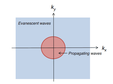
Suppose that an electromagnetic wave with wavevector $\boldsymbol{k}1=\left(k_x, 0,-k{1 z}\right)$ propagates in the negative $z$-direction and impinges on the interface. Because of the continuity of the tangential electromagnetic fields, the parallel component $k_x$ of the wavevector must be conserved at the interface. The $z$-component of the wavevector in the metal is determined from the dispersion relation
$$
k_x^2+k_{2 z}^2=\varepsilon_2 \mu_0 \omega^2
$$
Because of $\varepsilon_2<0$, the right-hand side of the equation is negative and we immediately find $k_{2 z}^2<0$, which can only be fulfilled for an imaginary wavenumber $k_{2 z}$. In other words, inside the metal the wave cannot propagate but has an evanescent character with an amplitude that decays exponentially when moving away from the interface. As a result, a wave impinging from the dielectric side on the metal becomes reflected, with only small losses due to ohmic dissipation caused by the exponentially decaying fields inside the metal. In Sect. 8.3.3 we will provide a more thorough discussion of this reflection.

From this analysis it seems that the dielectric-metal interface is a boring object. Fortunately, this hasty judgement is not true. We will show next that a novel type of wave exists at metal-dielectric interfaces, so-called surface plasmons, which are bound to the interface and have to be excited optically in a specific manner. In fact, we can distinguish two kinds of guided modes, namely
Transverse magnetic (TM): $\quad \boldsymbol{H}=H_y \hat{\boldsymbol{y}}$ is parallel to interface
Transverse electric (TE): $\quad \boldsymbol{E}=E_y \hat{\boldsymbol{y}}$ is parallel to interface.

物理代写|量子光学代写Quantum Optics代考|Kretschmann and Otto Geometry

In the previous section we have discussed that at the interface between a metal and a dielectric a novel type of excitations exists, so-called surface plasmons, associated with coherent surface charge excitations bound to light fields. However, we have also seen that these surface plasmons cannot be excited directly by optical means, or, as Harry Atwater has expressed it carefully, can only be excited “under the right circumstances.” To understand what these right circumstances are, we first analyze energy and momentum conservation in an optical excitation process.

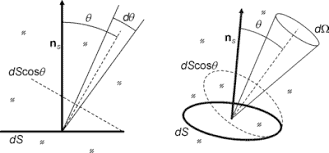
Light carries energy and momentum. In the following we adopt a photon language where the photon carries energy $\hbar \omega$ and momentum $\hbar \boldsymbol{k}$, but our reasoning works equally well for a purely classical electromagnetic description. Consider light oscillating with angular frequency $\omega$ and propagating in a medium with dielectric constant $\varepsilon_1$ that impinges on a metal surface located at $z=0$. The momentum carried by the photon is
$$
\hbar \boldsymbol{k}=[\sin \theta \hat{\boldsymbol{x}}+\cos \theta \hat{z}] \frac{\hbar k_0}{n_1},
$$
where $\theta$ is the angle of the incoming light with respect to the $z$-axis, $k_0=\frac{\omega}{c}$, and $n_1$ is the refractive index of the dielectric medium. In order to excite a surface plasmon the following quantities must be conserved:

• $\operatorname{energy} \hbar \omega$
• parallel momentum $\hbar k_x=\left(\hbar k_0 / n_1\right) \sin \theta$.
  Note that for the slab structure the translational symmetry along $z$ is broken and according to Noether’s theorem the momentum along $z$ is not conserved.

量子光学代考

物理代写|量子光学代写Quantum Optics代考|Surface Plasmons

考虑如图 8.1 所示的两种媒体之间的接口。上层是具有介电常数的电介质 $\varepsilon_1>0$, 较低的是一种具有负介 电常数的金属 $\varepsilon_2<0$. 为了简单起见，下面我们忽略虚部 $\varepsilon_2$ 并在最后讨论有损材料的影响。两种材料的磁 导率都设置为 $\mu_0$. – directionandimpingesontheinter face. Becauseofthecontinuityofthetangentialelect k_xofthewavevectormustbeconservedattheinter face. The和

• componentofthewavevectorinthemetalisdetermined fromthedispersionrelation $k_x^2+k_{2 z}^2=\varepsilon_2 \mu_0 \omega^2$ Becauseof ivarepsilon_2<0
  , theright – handsideoftheequationisnegativeandweimmediatelyfind $\left.\mathrm{k}{_}{2 \mathrm{z}}\right}^{\wedge} 2<0$ , whichcanonlybefulfilled foranimaginarywavenumberk ${2$ z $}$ \$。换句话说，在金属内部， 波不能传播，但具有渐逝特性，其振幅在远离界面时呈指数衰减。结果，从电介质侧撞击到金属上的波被 反射，由于金属内部呈指数衰减的场引起的欧姆耗散，只有很小的损失。昆虫。8.3.3 我们将对这种反思 进行更深入的讨论。
  从这个分析看来，介电金属界面是一个无聊的对象。幸运的是，这种仓促的判断并不正确。接下来我们将 展示一种新型的波存在于金属-电介质界面，即所谓的表面等离子体激元，它与界面结合并且必须以特定 方式进行光学激发。其实我们可以区分两种导模，即 横磁 (TM) : $\quad \boldsymbol{H}=H_y \hat{\boldsymbol{y}}$
  与接口横向电 (TE)平行: $\boldsymbol{E}=E_y \hat{\boldsymbol{y}}$ 与接口平行。

物理代写|量子光学代写Quantum Optics代考|Kretschmann and Otto Geometry

在上一节中，我们讨论了在金属和电介质之间的界面处存在一种新型的激发，即所谓的表面等离子体激 元，与束缚于光场的相干表面电荷激发有关。然而，我们也看到，这些表面等离子激元不能通过光学手段 直接激发，或者正如哈里·阿特沃特 (Harry Atwater) 仔细表述的那样，只能“在适当的情况下”激发。为了 理解这些正确的情况是什么，我们首先分析光激发过程中的能量和动量守恒。
光携带能量和动量。下面我们采用光子语言，其中光子携带能量 $\hbar \omega$ 和势头 $\hbar k$ ，但我们的推理同样适用于 纯经典电磁描述。考虑以角频率振荡的光 $\omega$ 并在具有介电常数的介质中传播唕撞击位于的金属表面 $z=0$. 光子携带的动量是
$$
\hbar \boldsymbol{k}=[\sin \theta \hat{\boldsymbol{x}}+\cos \theta \hat{z}] \frac{\hbar k_0}{n_1},
$$
在哪里 $\theta$ 是入射光相对于 $z$-轴， $k_0=\frac{\omega}{c}$ ，和 $n_1$ 是电介质的折射率。为了激发表面等离子体激元，必须守 恒以下量：

• energy $\hbar \omega$
• 平行矩 $\hbar k_x=\left(\hbar k_0 / n_1\right) \sin \theta$.
  请注意，对于平板结构，平移对称性沿 $z$ 被打破了，根据诺特定理，动量沿着 $z$ 不守恒。

统计代写请认准statistics-lab™. statistics-lab™为您的留学生涯保驾护航。

金融工程代写

金融工程是使用数学技术来解决金融问题。金融工程使用计算机科学、统计学、经济学和应用数学领域的工具和知识来解决当前的金融问题，以及设计新的和创新的金融产品。

非参数统计代写

非参数统计指的是一种统计方法，其中不假设数据来自于由少数参数决定的规定模型；这种模型的例子包括正态分布模型和线性回归模型。

广义线性模型代考

广义线性模型（GLM）归属统计学领域，是一种应用灵活的线性回归模型。该模型允许因变量的偏差分布有除了正态分布之外的其它分布。

术语 广义线性模型（GLM）通常是指给定连续和/或分类预测因素的连续响应变量的常规线性回归模型。它包括多元线性回归，以及方差分析和方差分析（仅含固定效应）。

有限元方法代写

有限元方法（FEM）是一种流行的方法，用于数值解决工程和数学建模中出现的微分方程。典型的问题领域包括结构分析、传热、流体流动、质量运输和电磁势等传统领域。

有限元是一种通用的数值方法，用于解决两个或三个空间变量的偏微分方程（即一些边界值问题）。为了解决一个问题，有限元将一个大系统细分为更小、更简单的部分，称为有限元。这是通过在空间维度上的特定空间离散化来实现的，它是通过构建对象的网格来实现的：用于求解的数值域，它有有限数量的点。边界值问题的有限元方法表述最终导致一个代数方程组。该方法在域上对未知函数进行逼近。[1] 然后将模拟这些有限元的简单方程组合成一个更大的方程系统，以模拟整个问题。然后，有限元通过变化微积分使相关的误差函数最小化来逼近一个解决方案。

tatistics-lab作为专业的留学生服务机构，多年来已为美国、英国、加拿大、澳洲等留学热门地的学生提供专业的学术服务，包括但不限于Essay代写，Assignment代写，Dissertation代写，Report代写，小组作业代写，Proposal代写，Paper代写，Presentation代写，计算机作业代写，论文修改和润色，网课代做，exam代考等等。写作范围涵盖高中，本科，研究生等海外留学全阶段，辐射金融，经济学，会计学，审计学，管理学等全球99%专业科目。写作团队既有专业英语母语作者，也有海外名校硕博留学生，每位写作老师都拥有过硬的语言能力，专业的学科背景和学术写作经验。我们承诺100%原创，100%专业，100%准时，100%满意。

随机分析代写

随机微积分是数学的一个分支，对随机过程进行操作。它允许为随机过程的积分定义一个关于随机过程的一致的积分理论。这个领域是由日本数学家伊藤清在第二次世界大战期间创建并开始的。

时间序列分析代写

随机过程，是依赖于参数的一组随机变量的全体，参数通常是时间。 随机变量是随机现象的数量表现，其时间序列是一组按照时间发生先后顺序进行排列的数据点序列。通常一组时间序列的时间间隔为一恒定值（如1秒，5分钟，12小时，7天，1年），因此时间序列可以作为离散时间数据进行分析处理。研究时间序列数据的意义在于现实中，往往需要研究某个事物其随时间发展变化的规律。这就需要通过研究该事物过去发展的历史记录，以得到其自身发展的规律。

回归分析代写

多元回归分析渐进（Multiple Regression Analysis Asymptotics）属于计量经济学领域，主要是一种数学上的统计分析方法，可以分析复杂情况下各影响因素的数学关系，在自然科学、社会和经济学等多个领域内应用广泛。

MATLAB代写

MATLAB 是一种用于技术计算的高性能语言。它将计算、可视化和编程集成在一个易于使用的环境中，其中问题和解决方案以熟悉的数学符号表示。典型用途包括：数学和计算算法开发建模、仿真和原型制作数据分析、探索和可视化科学和工程图形应用程序开发，包括图形用户界面构建MATLAB 是一个交互式系统，其基本数据元素是一个不需要维度的数组。这使您可以解决许多技术计算问题，尤其是那些具有矩阵和向量公式的问题，而只需用 C 或 Fortran 等标量非交互式语言编写程序所需的时间的一小部分。MATLAB 名称代表矩阵实验室。MATLAB 最初的编写目的是提供对由 LINPACK 和 EISPACK 项目开发的矩阵软件的轻松访问，这两个项目共同代表了矩阵计算软件的最新技术。MATLAB 经过多年的发展，得到了许多用户的投入。在大学环境中，它是数学、工程和科学入门和高级课程的标准教学工具。在工业领域，MATLAB 是高效研究、开发和分析的首选工具。MATLAB 具有一系列称为工具箱的特定于应用程序的解决方案。对于大多数 MATLAB 用户来说非常重要，工具箱允许您学习和应用专业技术。工具箱是 MATLAB 函数（M 文件）的综合集合，可扩展 MATLAB 环境以解决特定类别的问题。可用工具箱的领域包括信号处理、控制系统、神经网络、模糊逻辑、小波、仿真等。

R语言代写	问卷设计与分析代写
PYTHON代写	回归分析与线性模型代写
MATLAB代写	方差分析与试验设计代写
STATA代写	机器学习/统计学习代写
SPSS代写	计量经济学代写
EVIEWS代写	时间序列分析代写
EXCEL代写	深度学习代写
SQL代写	各种数据建模与可视化代写

如果你也在 怎样代写量子光学Quantum Optics这个学科遇到相关的难题，请随时右上角联系我们的24/7代写客服。

量子光学是原子、分子和光学物理学的一个分支，处理单个光量子（称为光子）如何与原子和分子相互作用。它包括研究光子的类似粒子的特性。

statistics-lab™ 为您的留学生涯保驾护航 在代写量子光学Quantum Optics方面已经树立了自己的口碑, 保证靠谱, 高质且原创的统计Statistics代写服务。我们的专家在代写量子光学Quantum Optics代写方面经验极为丰富，各种代写量子光学Quantum Optics相关的作业也就用不着说。

我们提供的量子光学Quantum Optics及其相关学科的代写，服务范围广, 其中包括但不限于:

• Statistical Inference 统计推断
• Statistical Computing 统计计算
• Advanced Probability Theory 高等概率论
• Advanced Mathematical Statistics 高等数理统计学
• (Generalized) Linear Models 广义线性模型
• Statistical Machine Learning 统计机器学习
• Longitudinal Data Analysis 纵向数据分析
• Foundations of Data Science 数据科学基础

物理代写|量子光学代写Quantum Optics代考|Kramers–Kronig Relation

For a response nonlocal in time, the dielectric displacement is related to the electric field through
$$
\boldsymbol{D}(\boldsymbol{r}, t)=\varepsilon_0\left{\boldsymbol{E}(\boldsymbol{r}, t)+\int_0^{\infty} \chi_e(\boldsymbol{r}, \tau) \boldsymbol{E}(\boldsymbol{r}, t-\tau) d \tau\right} .
$$
The important point about this expression is that only fields in the past contribute to the system’s response, and thus causality is fulfilled. As we will discuss in this section, as a consequence of this there exists a strict relation between the real and imaginary parts of the permittivity, the so-called Kramers-Kronig relation, and from the knowledge of the real part one can obtain the imaginary part and vice versa. The derivation of the relation is quite general, and the only ingredients needed are causality and linearity of the response.
From the Fourier transform of the above equation we find
$$
\varepsilon(\omega) / \varepsilon_0=1+\int_0^{\infty} e^{i \omega \tau} \chi_e(\tau) d \tau
$$
where from now on we suppress the $r$ dependence of $\chi_e$. Taking the complex conjugate of this, we can establish a relation between positive and negative frequencies $$
\varepsilon^(\omega) / \varepsilon_0=\varepsilon\left(-\omega^\right) / \varepsilon_0,
$$
where we have considered complex frequencies for reasons to become clear in a moment. In what follows, we will need an important theorem from complex analysis, the so-called Cauchy’s theorem, which we briefly discuss in Appendix A. It states that an integration in the complex plane along a closed contour $\mathcal{C}$ gives zero if the integrand is analytic within $\mathcal{C}$. In the following we apply Cauchy’s theorem to the response function
$$
\chi_e(z)=\int_0^{\infty} e^{i z \tau} \chi_e(\tau) d \tau
$$
where we have considered a complex frequency $z$. When $\chi_e(\omega)$ exists for real frequencies, nothing severe can happen when extending the frequencies to the upper complex plane with $z^{\prime \prime}>0$. There, the exponential reads
$$
e^{i\left(z^{\prime}+i z^{\prime \prime}\right) \tau}=e^{i z^{\prime} \tau} e^{-z^{\prime \prime} \tau}
$$

物理代写|量子光学代写Quantum Optics代考|Reciprocity Theorem in Optics

There exists an important theorem in optics, the so-called reciprocity theorem, from which one can derive a symmetry relation for the Green’s dyadics. Suppose that

• $\boldsymbol{J}_1$ is a current distribution which produces the fields $\boldsymbol{E}_1, \boldsymbol{H}_1$ and
• $J_2$ is a current distribution which produces the fields $\boldsymbol{E}_2, \boldsymbol{H}_2$.
  Then, one can derive the (Lorentz) reciprocity theorem
  Reciprocity Theorem of Optics
  $$
  \int \boldsymbol{J}_1 \cdot \boldsymbol{E}_2 d^3 r=\int \boldsymbol{J}_2 \cdot \boldsymbol{E}_1 d^3 r
  $$
  Here we assume that the integrals extend over the entire space. This theorem states that the relationship between an oscillating current distribution and the resulting electric field is unchanged if one interchanges the points where the current is placed and where the field is measured.

To prove the theorem, in the following we consider materials with frequencydependent and anisotropic permittivites and permeabilites $\overline{\bar{\varepsilon}}, \overline{\bar{\mu}}$. The curl equations of Maxwell’s equations then read
$$
\nabla \times \boldsymbol{E}=i \omega \overline{\bar{\mu}} \cdot \boldsymbol{H}, \quad \nabla \times \boldsymbol{H}=\boldsymbol{J}-i \omega \overline{\bar{\varepsilon}} \cdot \boldsymbol{E},
$$
where for simplicity we do not indicate the spatial and frequency dependence of the fields and material parameters. We next consider the vector identity $\nabla \cdot(\boldsymbol{E} \times \boldsymbol{H})=\boldsymbol{H} \cdot(\nabla \times \boldsymbol{E})-\boldsymbol{E} \cdot(\nabla \times \boldsymbol{H})$

量子光学代考

物理代写|量子光学代写Quantum Optics代考|Kramers–Kronig Relation

对于非局部时间响应，介电位移通过以下方式与电场相关
这个表达式的重点是，只有过去的字段有助于系统的响应，因此因果关系得到满足。正如我们将在本节中 讨论的那样，因此在介电常数的实部和虚部之间存在严格的关系，即所谓的 Kramers-Kronig 关系，并且 根据实部的知识，我们可以获得虚部部分，反之亦然。关系的推导非常普遍，唯一需要的成分是响应的因 果关系和线性。
由上式的傅里叶变换我们发现
$$
\varepsilon(\omega) / \varepsilon_0=1+\int_0^{\infty} e^{i \omega \tau} \chi_e(\tau) d \tau
$$
从现在开始我们压制 $r$ 的依赖 $\chi_e$. 取其复共轭，我们可以建立正负频率之间的关系
我们考虑复杂频率的原因稍后会变得清晰。接下来，我们将需要复分析中的一个重要定理，即所谓的柯西 定理，我们将在附录 $\mathrm{A}$ 中对其进行简要讨论。它指出复平面中沿闭合轮廓的积分C如果被积函数在内部是 解析的，则给出零 $\mathcal{C}$. 下面我们将柯西定理应用于响应函数
$$
\chi_e(z)=\int_0^{\infty} e^{i z \tau} \chi_e(\tau) d \tau
$$
我们考虑了一个复杂的频率 $z$. 什么时候 $\chi_e(\omega)$ 对于实频率存在，当将频率扩展到上复平面时，不会发生 任何严重的事情 $z^{\prime \prime}>0$. 在那里，指数读数
$$
e^{i\left(z^{\prime}+i z^{\prime \prime}\right) \tau}=e^{i z^{\prime} \tau} e^{-z^{\prime \prime} \tau}
$$

物理代写|量子光学代写Quantum Optics代考|Reciprocity Theorem in Optics

光学中有一个重要的定理，即所谓的互易定理，从中可以推导出格林并矢的对称关系。假设

• $\boldsymbol{J}_1$ 是产生场的电流分布 $\boldsymbol{E}_1, \boldsymbol{H}_1$ 和
• $J_2$ 是产生场的电流分布 $\boldsymbol{E}_2, \boldsymbol{H}_2$.
  然后，可以推导出 (洛伦兹) 互易定理
  Reciprocity Theorem of Optics
  $$
  \int \boldsymbol{J}_1 \cdot \boldsymbol{E}_2 d^3 r=\int \boldsymbol{J}_2 \cdot \boldsymbol{E}_1 d^3 r
  $$
  这里我们假设积分延伸到整个空间。该定理指出，如果互换放置电流的点和测量场的点，则振荡电 流分布与产生的电场之间的关系不会改变。
  为了证明该定理，下面我们考虑具有频率相关和各向异性介电常数和磁导率的材料 $\overline{\bar{\varepsilon}}, \overline{\bar{\mu}}$. 然后读取麦克斯 韦方程组的旋度方程
  $$
  \nabla \times \boldsymbol{E}=i \omega \overline{\bar{\mu}} \cdot \boldsymbol{H}, \quad \nabla \times \boldsymbol{H}=\boldsymbol{J}-i \omega \overline{\bar{\varepsilon}} \cdot \boldsymbol{E}
  $$
  其中为简单起见，我们没有指出场和材料参数的空间和频率依赖性。接下来我们考虑向量恒等式
  $$
  \nabla \cdot(\boldsymbol{E} \times \boldsymbol{H})=\boldsymbol{H} \cdot(\nabla \times \boldsymbol{E})-\boldsymbol{E} \cdot(\nabla \times \boldsymbol{H})
  $$

统计代写请认准statistics-lab™. statistics-lab™为您的留学生涯保驾护航。

金融工程代写

金融工程是使用数学技术来解决金融问题。金融工程使用计算机科学、统计学、经济学和应用数学领域的工具和知识来解决当前的金融问题，以及设计新的和创新的金融产品。

非参数统计代写

非参数统计指的是一种统计方法，其中不假设数据来自于由少数参数决定的规定模型；这种模型的例子包括正态分布模型和线性回归模型。

广义线性模型代考

广义线性模型（GLM）归属统计学领域，是一种应用灵活的线性回归模型。该模型允许因变量的偏差分布有除了正态分布之外的其它分布。

术语 广义线性模型（GLM）通常是指给定连续和/或分类预测因素的连续响应变量的常规线性回归模型。它包括多元线性回归，以及方差分析和方差分析（仅含固定效应）。

有限元方法代写

有限元方法（FEM）是一种流行的方法，用于数值解决工程和数学建模中出现的微分方程。典型的问题领域包括结构分析、传热、流体流动、质量运输和电磁势等传统领域。

有限元是一种通用的数值方法，用于解决两个或三个空间变量的偏微分方程（即一些边界值问题）。为了解决一个问题，有限元将一个大系统细分为更小、更简单的部分，称为有限元。这是通过在空间维度上的特定空间离散化来实现的，它是通过构建对象的网格来实现的：用于求解的数值域，它有有限数量的点。边界值问题的有限元方法表述最终导致一个代数方程组。该方法在域上对未知函数进行逼近。[1] 然后将模拟这些有限元的简单方程组合成一个更大的方程系统，以模拟整个问题。然后，有限元通过变化微积分使相关的误差函数最小化来逼近一个解决方案。

tatistics-lab作为专业的留学生服务机构，多年来已为美国、英国、加拿大、澳洲等留学热门地的学生提供专业的学术服务，包括但不限于Essay代写，Assignment代写，Dissertation代写，Report代写，小组作业代写，Proposal代写，Paper代写，Presentation代写，计算机作业代写，论文修改和润色，网课代做，exam代考等等。写作范围涵盖高中，本科，研究生等海外留学全阶段，辐射金融，经济学，会计学，审计学，管理学等全球99%专业科目。写作团队既有专业英语母语作者，也有海外名校硕博留学生，每位写作老师都拥有过硬的语言能力，专业的学科背景和学术写作经验。我们承诺100%原创，100%专业，100%准时，100%满意。

随机分析代写

随机微积分是数学的一个分支，对随机过程进行操作。它允许为随机过程的积分定义一个关于随机过程的一致的积分理论。这个领域是由日本数学家伊藤清在第二次世界大战期间创建并开始的。

时间序列分析代写

随机过程，是依赖于参数的一组随机变量的全体，参数通常是时间。 随机变量是随机现象的数量表现，其时间序列是一组按照时间发生先后顺序进行排列的数据点序列。通常一组时间序列的时间间隔为一恒定值（如1秒，5分钟，12小时，7天，1年），因此时间序列可以作为离散时间数据进行分析处理。研究时间序列数据的意义在于现实中，往往需要研究某个事物其随时间发展变化的规律。这就需要通过研究该事物过去发展的历史记录，以得到其自身发展的规律。

回归分析代写

多元回归分析渐进（Multiple Regression Analysis Asymptotics）属于计量经济学领域，主要是一种数学上的统计分析方法，可以分析复杂情况下各影响因素的数学关系，在自然科学、社会和经济学等多个领域内应用广泛。

MATLAB代写

MATLAB 是一种用于技术计算的高性能语言。它将计算、可视化和编程集成在一个易于使用的环境中，其中问题和解决方案以熟悉的数学符号表示。典型用途包括：数学和计算算法开发建模、仿真和原型制作数据分析、探索和可视化科学和工程图形应用程序开发，包括图形用户界面构建MATLAB 是一个交互式系统，其基本数据元素是一个不需要维度的数组。这使您可以解决许多技术计算问题，尤其是那些具有矩阵和向量公式的问题，而只需用 C 或 Fortran 等标量非交互式语言编写程序所需的时间的一小部分。MATLAB 名称代表矩阵实验室。MATLAB 最初的编写目的是提供对由 LINPACK 和 EISPACK 项目开发的矩阵软件的轻松访问，这两个项目共同代表了矩阵计算软件的最新技术。MATLAB 经过多年的发展，得到了许多用户的投入。在大学环境中，它是数学、工程和科学入门和高级课程的标准教学工具。在工业领域，MATLAB 是高效研究、开发和分析的首选工具。MATLAB 具有一系列称为工具箱的特定于应用程序的解决方案。对于大多数 MATLAB 用户来说非常重要，工具箱允许您学习和应用专业技术。工具箱是 MATLAB 函数（M 文件）的综合集合，可扩展 MATLAB 环境以解决特定类别的问题。可用工具箱的领域包括信号处理、控制系统、神经网络、模糊逻辑、小波、仿真等。

R语言代写	问卷设计与分析代写
PYTHON代写	回归分析与线性模型代写
MATLAB代写	方差分析与试验设计代写
STATA代写	机器学习/统计学习代写
SPSS代写	计量经济学代写
EVIEWS代写	时间序列分析代写
EXCEL代写	深度学习代写
SQL代写	各种数据建模与可视化代写

如果你也在 怎样代写量子光学Quantum Optics这个学科遇到相关的难题，请随时右上角联系我们的24/7代写客服。

量子光学是原子、分子和光学物理学的一个分支，处理单个光量子（称为光子）如何与原子和分子相互作用。它包括研究光子的类似粒子的特性。

statistics-lab™ 为您的留学生涯保驾护航 在代写量子光学Quantum Optics方面已经树立了自己的口碑, 保证靠谱, 高质且原创的统计Statistics代写服务。我们的专家在代写量子光学Quantum Optics代写方面经验极为丰富，各种代写量子光学Quantum Optics相关的作业也就用不着说。

我们提供的量子光学Quantum Optics及其相关学科的代写，服务范围广, 其中包括但不限于:

• Statistical Inference 统计推断
• Statistical Computing 统计计算
• Advanced Probability Theory 高等概率论
• Advanced Mathematical Statistics 高等数理统计学
• (Generalized) Linear Models 广义线性模型
• Statistical Machine Learning 统计机器学习
• Longitudinal Data Analysis 纵向数据分析
• Foundations of Data Science 数据科学基础

物理代写|量子光学代写Quantum Optics代考|Connection to Dielectric Media

Recall that the polarization density $\mathbf{P}$ is the dipole moment per unit volume. Thus, for an atomic vapor of number density $N$,
$$
\mathbf{P}^{(+)}=N \mathbf{d}^{(+)}=N \alpha(\omega) \mathbf{E}^{(+)}=\hat{\varepsilon} \frac{N e^2 / m}{\omega_0^2-\omega^2} E_0^{(+)} e^{-i \omega t} .
$$
This expression is valid for a rarefied medium, where the interactions between the atoms are negligible. In dense media, correlations between dipoles cause deviations from these results. We can thus write the susceptibility for the vapor as
$$
\chi(\omega)=\frac{N e^2 / m \epsilon_0}{\omega_0^2-\omega^2},
$$
(classical susceptibility)
in view of the defining relation $\mathbf{P}=\epsilon_0 \chi \mathbf{E}$. Keeping the polarizability as the fundamental microscopic quantity, we can of course also write
$$
\chi(\omega)=\frac{N}{\epsilon_0} \alpha(\omega)
$$
(susceptibility-polarizability relation)
for the susceptibility of a vapor of number density $N$ in terms of the polarizability.

物理代写|量子光学代写Quantum Optics代考|Lorentz Model

A better model of the atom is a damped harmonic oscillator. This improved model is known as the Lorentz model of the atom, and the equation of motion is
$$
m \ddot{\mathbf{x}}^{(+)}+m \gamma \dot{\mathbf{x}}^{(+)}+m \omega_0^2 \mathbf{x}^{(+)}=-\hat{\varepsilon} e E_0^{(+)} e^{-i \omega t} .
$$
(Lorentz model)
The damping (“friction”) term models radiation reaction due to the charge acceleration (the classical analogue of spontaneous emission) and collisions with other atoms. A quantum-mechanical calculation shows that for an isolated atom, the damping rate is the same as the Einstein $A$ coefficient (spontaneous emission rate): $\gamma=A_{21}$

Again, we assume a solution of the form $\mathbf{x}^{(+)}(t)=\hat{\varepsilon} x_0^{(+)} e^{-i \omega t}$. Following the method above, the solution is
$$
x_0^{(+)}=\frac{e E_0^{(+)} / m}{\omega^2-\omega_0^2+i \gamma \omega} .
$$
Now the displacement is complex, reflecting a phase lag of the displacement behind the field, with phase angle
$$
\delta=\tan ^{-1}\left(\frac{\gamma \omega}{\omega_0^2-\omega^2}\right)
$$

The phase lag approaches zero for $\omega \ll \omega_0$ and $\pi$ for $\omega \gg \omega_0(\delta=\pi / 2$ exactly on resonance). Then for this case, the polarizability becomes
$$
\alpha(\omega)=\frac{e^2 / m}{\omega_0^2-\omega^2-i \gamma \omega} .
$$
(polarizability with damping)
The susceptibility likewise becomes
$$
\chi(\omega)=\frac{N e^2 / m \epsilon_0}{\omega_0^2-\omega^2-i \gamma \omega} .
$$
(susceptibility with damping)
It is worth reiterating here that $\alpha$ and $\chi$ are complex quantities defined for the positive-rotating fields via $\mathbf{d}^{(+)}=\alpha(\omega) \mathbf{E}^{(+)}$and $\mathbf{P}^{(+)}=\epsilon_0 \chi \mathbf{E}^{(+)}$, and therefore must be treated appropriately.
If $\chi$ is small (as for a dilute vapor), the complex refractive index is
$$
\tilde{n}(\omega)=\sqrt{1+\chi(\omega)} \approx 1+\frac{\chi(\omega)}{2}=1+\frac{N e^2}{2 m \epsilon_0} \frac{\left(\omega_0^2-\omega^2\right)}{\left(\omega_0^2-\omega^2\right)^2+\gamma^2 \omega^2}+i \frac{N e^2}{2 m \epsilon_0} \frac{\gamma \omega}{\left(\omega_0^2-\omega^2\right)^2+\gamma^2 \omega^2} .
$$

量子光学代考

物理代写|量子光学代写Quantum Optics代考|Connection to Dielectric Media

回想一下极化密度 $\mathbf{P}$ 是每单位体积的偶极矩。因此，对于数密度的原子蒸汽 $N$ ，
$$
\mathbf{P}^{(+)}=N \mathbf{d}^{(+)}=N \alpha(\omega) \mathbf{E}^{(+)}=\hat{\varepsilon} \frac{N e^2 / m}{\omega_0^2-\omega^2} E_0^{(+)} e^{-i \omega t} .
$$
该表达式适用于稀薄介质，其中原子之间的相互作用可以忽略不计。在致密介质中，偶极子之间的相关 性导致与这些结果的偏差。因此，我们可以将蒸汽的磁化率写为
$$
\chi(\omega)=\frac{N e^2 / m \epsilon_0}{\omega_0^2-\omega^2}
$$
(经典敏感性)
鉴于定义关系 $\mathbf{P}=\epsilon_0 \chi \mathbf{E}$. 保持极化率作为基本的微观量，我们当然也可以写成
$$
\chi(\omega)=\frac{N}{\epsilon_0} \alpha(\omega)
$$
(磁化率-极化率关系)
对于数密度蒸气的磁化率 $N$ 在极化率方面。

物理代写|量子光学代写Quantum Optics代考|Lorentz Model

一个更好的原子模型是阻尼谐振子。这种改进的模型被称为原子的洛伦兹模型，运动方程为
$$
m \ddot{\mathbf{x}}^{(+)}+m \gamma \dot{\mathbf{x}}^{(+)}+m \omega_0^2 \mathbf{x}^{(+)}=-\hat{\varepsilon} e E_0^{(+)} e^{-i \omega t}
$$
(洛伦兹模型)
阻尼 (“摩擦”) 项模拟由于电荷加速（自发辐射的经典模拟) 和与其他原子碰撞引起的辐射反应。量子 力学计算表明，对于一个孤立的原子，阻尼率与爱因斯坦相同 $A$ 系数 (自发辐射率) : $\gamma=A_{21}$
同样，我们假设一个形式的解决方案 $\mathbf{x}^{(+)}(t)=\hat{\varepsilon} x_0^{(+)} e^{-i \omega t}$. 按照上面的方法，解决方法是
$$
x_0^{(+)}=\frac{e E_0^{(+)} / m}{\omega^2-\omega_0^2+i \gamma \omega} .
$$
现在位移很复杂，反映了场后位移的相位滞后，具有相位角
$$
\delta=\tan ^{-1}\left(\frac{\gamma \omega}{\omega_0^2-\omega^2}\right)
$$
相位滞后接近于零 $\omega \ll \omega_0$ 和 $\pi$ 为了 $\omega \gg \omega_0(\delta=\pi / 2$ 正好在共振上）。那么对于这种情况，极化率变 为
$$
\alpha(\omega)=\frac{e^2 / m}{\omega_0^2-\omega^2-i \gamma \omega}
$$
(带阻尼的极化率)
磁化率同样变为
$$
\chi(\omega)=\frac{N e^2 / m \epsilon_0}{\omega_0^2-\omega^2-i \gamma \omega}
$$
(阻尼敏感性)
这里值得重申的是 $\alpha$ 和 $\chi$ 是为正旋转场定义的复数，通过 $\mathbf{d}^{(+)}=\alpha(\omega) \mathbf{E}^{(+)}$和 $\mathbf{P}^{(+)}=\epsilon_0 \chi \mathbf{E}^{(+)}$，因 此必须适当对待。
如果 $\chi$ 很小 (对于稀蒸汽)，复折射率为
$$
\tilde{n}(\omega)=\sqrt{1+\chi(\omega)} \approx 1+\frac{\chi(\omega)}{2}=1+\frac{N e^2}{2 m \epsilon_0} \frac{\left(\omega_0^2-\omega^2\right)}{\left(\omega_0^2-\omega^2\right)^2+\gamma^2 \omega^2}+i \frac{N e^2}{2 m \epsilon_0} \frac{\gamma \omega}{\left(\omega_0^2-\omega^2\right)^2+\gamma^2}
$$

统计代写请认准statistics-lab™. statistics-lab™为您的留学生涯保驾护航。

金融工程代写

金融工程是使用数学技术来解决金融问题。金融工程使用计算机科学、统计学、经济学和应用数学领域的工具和知识来解决当前的金融问题，以及设计新的和创新的金融产品。

非参数统计代写

非参数统计指的是一种统计方法，其中不假设数据来自于由少数参数决定的规定模型；这种模型的例子包括正态分布模型和线性回归模型。

广义线性模型代考

广义线性模型（GLM）归属统计学领域，是一种应用灵活的线性回归模型。该模型允许因变量的偏差分布有除了正态分布之外的其它分布。

术语 广义线性模型（GLM）通常是指给定连续和/或分类预测因素的连续响应变量的常规线性回归模型。它包括多元线性回归，以及方差分析和方差分析（仅含固定效应）。

有限元方法代写

有限元方法（FEM）是一种流行的方法，用于数值解决工程和数学建模中出现的微分方程。典型的问题领域包括结构分析、传热、流体流动、质量运输和电磁势等传统领域。

有限元是一种通用的数值方法，用于解决两个或三个空间变量的偏微分方程（即一些边界值问题）。为了解决一个问题，有限元将一个大系统细分为更小、更简单的部分，称为有限元。这是通过在空间维度上的特定空间离散化来实现的，它是通过构建对象的网格来实现的：用于求解的数值域，它有有限数量的点。边界值问题的有限元方法表述最终导致一个代数方程组。该方法在域上对未知函数进行逼近。[1] 然后将模拟这些有限元的简单方程组合成一个更大的方程系统，以模拟整个问题。然后，有限元通过变化微积分使相关的误差函数最小化来逼近一个解决方案。

tatistics-lab作为专业的留学生服务机构，多年来已为美国、英国、加拿大、澳洲等留学热门地的学生提供专业的学术服务，包括但不限于Essay代写，Assignment代写，Dissertation代写，Report代写，小组作业代写，Proposal代写，Paper代写，Presentation代写，计算机作业代写，论文修改和润色，网课代做，exam代考等等。写作范围涵盖高中，本科，研究生等海外留学全阶段，辐射金融，经济学，会计学，审计学，管理学等全球99%专业科目。写作团队既有专业英语母语作者，也有海外名校硕博留学生，每位写作老师都拥有过硬的语言能力，专业的学科背景和学术写作经验。我们承诺100%原创，100%专业，100%准时，100%满意。

随机分析代写

随机微积分是数学的一个分支，对随机过程进行操作。它允许为随机过程的积分定义一个关于随机过程的一致的积分理论。这个领域是由日本数学家伊藤清在第二次世界大战期间创建并开始的。

时间序列分析代写

随机过程，是依赖于参数的一组随机变量的全体，参数通常是时间。 随机变量是随机现象的数量表现，其时间序列是一组按照时间发生先后顺序进行排列的数据点序列。通常一组时间序列的时间间隔为一恒定值（如1秒，5分钟，12小时，7天，1年），因此时间序列可以作为离散时间数据进行分析处理。研究时间序列数据的意义在于现实中，往往需要研究某个事物其随时间发展变化的规律。这就需要通过研究该事物过去发展的历史记录，以得到其自身发展的规律。

回归分析代写

多元回归分析渐进（Multiple Regression Analysis Asymptotics）属于计量经济学领域，主要是一种数学上的统计分析方法，可以分析复杂情况下各影响因素的数学关系，在自然科学、社会和经济学等多个领域内应用广泛。

MATLAB代写

MATLAB 是一种用于技术计算的高性能语言。它将计算、可视化和编程集成在一个易于使用的环境中，其中问题和解决方案以熟悉的数学符号表示。典型用途包括：数学和计算算法开发建模、仿真和原型制作数据分析、探索和可视化科学和工程图形应用程序开发，包括图形用户界面构建MATLAB 是一个交互式系统，其基本数据元素是一个不需要维度的数组。这使您可以解决许多技术计算问题，尤其是那些具有矩阵和向量公式的问题，而只需用 C 或 Fortran 等标量非交互式语言编写程序所需的时间的一小部分。MATLAB 名称代表矩阵实验室。MATLAB 最初的编写目的是提供对由 LINPACK 和 EISPACK 项目开发的矩阵软件的轻松访问，这两个项目共同代表了矩阵计算软件的最新技术。MATLAB 经过多年的发展，得到了许多用户的投入。在大学环境中，它是数学、工程和科学入门和高级课程的标准教学工具。在工业领域，MATLAB 是高效研究、开发和分析的首选工具。MATLAB 具有一系列称为工具箱的特定于应用程序的解决方案。对于大多数 MATLAB 用户来说非常重要，工具箱允许您学习和应用专业技术。工具箱是 MATLAB 函数（M 文件）的综合集合，可扩展 MATLAB 环境以解决特定类别的问题。可用工具箱的领域包括信号处理、控制系统、神经网络、模糊逻辑、小波、仿真等。

R语言代写	问卷设计与分析代写
PYTHON代写	回归分析与线性模型代写
MATLAB代写	方差分析与试验设计代写
STATA代写	机器学习/统计学习代写
SPSS代写	计量经济学代写
EVIEWS代写	时间序列分析代写
EXCEL代写	深度学习代写
SQL代写	各种数据建模与可视化代写

如果你也在 怎样代写量子光学Quantum Optics这个学科遇到相关的难题，请随时右上角联系我们的24/7代写客服。

量子光学是原子、分子和光学物理学的一个分支，处理单个光量子（称为光子）如何与原子和分子相互作用。它包括研究光子的类似粒子的特性。

statistics-lab™ 为您的留学生涯保驾护航 在代写量子光学Quantum Optics方面已经树立了自己的口碑, 保证靠谱, 高质且原创的统计Statistics代写服务。我们的专家在代写量子光学Quantum Optics代写方面经验极为丰富，各种代写量子光学Quantum Optics相关的作业也就用不着说。

我们提供的量子光学Quantum Optics及其相关学科的代写，服务范围广, 其中包括但不限于:

• Statistical Inference 统计推断
• Statistical Computing 统计计算
• Advanced Probability Theory 高等概率论
• Advanced Mathematical Statistics 高等数理统计学
• (Generalized) Linear Models 广义线性模型
• Statistical Machine Learning 统计机器学习
• Longitudinal Data Analysis 纵向数据分析
• Foundations of Data Science 数据科学基础

物理代写|量子光学代写Quantum Optics代考|Classical Atom–Field Interactions

We will now model the interaction between light and atoms, using a classical model of the atom. This will allow us to treat a variety of phenomena from the refractive index of atomic vapors to the conductivity of metals to laser cooling and trapping of atoms.

We will model the atom as a classical harmonic oscillator, an electron bound to the nucleus by a harmonic force (linear spring):
$$
m \ddot{\mathbf{x}}+m \omega_0^2 \mathbf{x}=0
$$
Here, $\mathbf{x}$ represents the average position of the electron, since quantum-mechanically, the electron is not localized, and $\omega_0$ is the resonant frequency of the harmonic potential. The above equation is also in centerof-mass coordinates, so that we can ignore the motion of the nucleus. Thus, $m$ is the reduced mass of the electron, given by
$$
m=\frac{m_{\mathrm{e}} m_{\mathrm{n}}}{m_{\mathrm{e}}+m_{\mathrm{n}}}
$$
where $m_{\mathrm{e}}$ is the electron mass, and $m_{\mathrm{n}}$ is the nuclear mass. Generally $m_{\mathrm{e}} \ll m_{\mathrm{n}}$, so
$$
m \approx m_{\mathrm{e}}\left(1-\frac{m_{\mathrm{e}}}{m_{\mathrm{n}}}\right),
$$
and generally, it is a good approximation to use $m \approx m_{\mathrm{e}}$.
Why use a classical calculation, when an atom is a manifestly quantum-mechanical object? It turns out that the classical calculation gets many phenomena correct, and these results can be justified by quantum calculations. Essentially, the classical calculation is good for weak atomic excitations, when the harmonic potential, the lowest-order approximation to an arbitrary potential, is an accurate model. (It is even a good approximation to treat the quantum electromagnetic field classically as long as many photons are present, since the field turns out to be a set of harmonic oscillators, which are “not very quantum-mechanical.” Then our requirement of weak excitation of the atom implies an atom-field coupling that is in some sense very weak; we will see that this is true when discussing the atomic cross section in Section 1.2.1.) In particular, the classical model does not predict any saturation effects, and as we will see, it requires a bit of patching to make it quantitatively correct, even in the limit of small intensity.

物理代写|量子光学代写Quantum Optics代考|Polarizability

We will now consider the interaction of the atom with a monochromatic field of the form
$$
\mathbf{E}^{(+)}(t)=\hat{\varepsilon} E_0^{(+)} e^{-i \omega t},
$$ where $\hat{\varepsilon}$ is the unit polarization vector. Here, we are using the complex notation for the field, where we separate according to the positive- and negative-frequency components:
$$
\begin{aligned}
\mathbf{E}(\mathbf{r}, t) & =\mathbf{E}(\mathbf{r}) \cos (\omega t+\phi) \
& =\mathbf{E}(\mathbf{r}) \frac{e^{-i \phi}}{2} e^{-i \omega t}+\mathbf{E}(\mathbf{r}) \frac{e^{i \phi}}{2} e^{i \omega t} \
& =: \mathbf{E}^{(+)}(\mathbf{r}) e^{-i \omega t}+\mathbf{E}^{(-)}(\mathbf{r}) e^{i \omega t}
\end{aligned}
$$
Recall that we are defining $\mathbf{E}^{( \pm)}$to go with $e^{\mp i \omega t}$, since by convention $e^{-i \omega t}$ corresponds to the positive frequency $\omega$ and $e^{i \omega t}=e^{-i(-\omega) t}$ corresponds to the negative frequency $(-\omega)$. The physical field is just the sum of the positive- and negative-frequency parts. But notice that these parts are complex conjugates, as is required to get a real (physical) field. Thus, we can always write the physical field as $E^{(+)}$with its conjugate:
$$
\mathbf{E}(\mathbf{r}, t)=\mathbf{E}^{(+)}(\mathbf{r}) e^{-i \omega t}+\text { c.c. }=2 \operatorname{Re}\left{\mathbf{E}^{(+)}(\mathbf{r}) e^{-i \omega t}\right} .
$$
Of course, we apply this notation to all other quantities driven by the field, such as the displacement of the electron that we consider below. Mathematically, it is simpler to keep only one part of the solution, but to obtain the physical result, you always need to add the complex conjugate (assuming that all the calculations are linear). Note that classically, this decomposition arises as a mathematical convenience. As we will see much later, in the quantum treatment of the field this decomposition is more fundamental and significant, since the two components will play the roles of photon creation and annihilation operators.

In writing down the expression (1.4), we are making the dipole approximation: we are assuming that the size of the atom is much smaller than the optical wavelength, so that the electron only sees the field at the nuclear position. Thus, we need not consider the spatial dependence or propagation direction of the field. The force on the electron due to the field is
$$
\mathbf{F}^{(+)}=-e \mathbf{E}^{(+)}
$$
where $e$ is the fundamental charge, the magnitude of the electron charge (so that the electron charge is $-e)$

量子光学代考

物理代写|量子光学代写Quantum Optics代考|Classical Atom–Field Interactions

我们现在将使用原子的经典模型来模拟光与原子之间的相互作用。这将使我们能够处理从原子蒸气的折 射率到金属的电导率再到激光冷却和原子捕获的各种现象。
我们将原子建模为经典谐振子，电子通过谐波力 (线性弹簧) 束缚在原子核上:
$$
m \ddot{\mathbf{x}}+m \omega_0^2 \mathbf{x}=0
$$
这里， $\mathbf{x}$ 代表电子的平均位置，因为在量子力学上，电子不是局域化的，并且 $\omega_0$ 是谐波电势的谐振频 率。上式也是在质心坐标下，所以我们可以忽略原子核的运动。因此， $m$ 是电子的约化质量，由下式给 出
$$
m=\frac{m_{\mathrm{e}} m_{\mathrm{n}}}{m_{\mathrm{e}}+m_{\mathrm{n}}}
$$
在哪里 $m_{\mathrm{e}}$ 是电子质量，和 $m_{\mathrm{n}}$ 是核质量。一般来说 $m_{\mathrm{e}} \ll m_{\mathrm{n}}$ ，所以
$$
m \approx m_{\mathrm{e}}\left(1-\frac{m_{\mathrm{e}}}{m_{\mathrm{n}}}\right),
$$
通常，它是一个很好的近似值 $m \approx m_{\mathrm{e}}$.
当原子明显是量子力学对象时，为什么要使用经典计算呢? 事实证明，经典计算对许多现象都是正确 的，而这些结果可以用量子计算来证明。本质上，当谐波势（任意势的最低阶近似值）是一个精确模型 时，经典计算适用于弱原子激发。（只要存在许多光子，经典地处理量子电磁场甚至是一个很好的近 似，因为该场结果是一组谐振子，“不是很量子力学”。那么我们的弱要求原子的激发意味着在某种意义 上非常弱的原子场耦合；我们将在 1.2.1 节讨论原子横截面时看到这是真的。）特别是，

物理代写|量子光学代写Quantum Optics代考|Polarizability

我们现在将考虑原子与形式的单色场的相互作用
$$
\mathbf{E}^{(+)}(t)=\hat{\varepsilon} E_0^{(+)} e^{-i \omega t}
$$
在哪里 $\hat{\varepsilon}$ 是单位偏振矢量。在这里，我们对字段使用复杂的表示法，我们根据正频率和负频率分量分 开:
$$
\mathbf{E}(\mathbf{r}, t)=\mathbf{E}(\mathbf{r}) \cos (\omega t+\phi) \quad=\mathbf{E}(\mathbf{r}) \frac{e^{-i \phi}}{2} e^{-i \omega t}+\mathbf{E}(\mathbf{r}) \frac{e^{i \phi}}{2} e^{i \omega t}=: \mathbf{E}^{(+)}(\mathbf{r}) e^{-i \omega t}+\mathbf{E}^{(-)}(\mathbf{r}) e^2
$$
回想一下，我们正在定义 $\mathbf{E}^{( \pm)}$一起去 $e^{\mp i \omega t}$ ，因为按照惯例 $e^{-i \omega t}$ 对应正频率 $\omega$ 和 $e^{i \omega t}=e^{-i(-\omega) t}$ 对应负 频率 $(-\omega)$. 物理场只是正频率部分和负频率部分的总和。但请注意，这些部分是复共轭，这是获得真实 (物理) 场所必需的。因此，我们总是可以将物理场写成 $E^{(+)}$及其共轭：
Imathbf ${E}}(\backslash m a t h b f{r}, t)=\backslash m a t h b f{E} \wedge{(+)}(\backslash m a t h b f{r}) e^{\wedge}{-i$ lomega t $}+\backslash t e x t{c c}=2$ loperatorname ${$ Re $} \backslash$ left ${\backslash m a t h b i$
当然，我们将此符号应用于场驱动的所有其他量，例如我们在下面考虑的电子位移。在数学上，只保留 一部分解比较简单，但要得到物理结果，总是需要加上复共轭（假设所有的计算都是线性的）。请注 意，经典地，这种分解是为了数学上的便利而出现的。正如我们稍后将看到的，在场的量子处理中，这 种分解更为基础和重要，因为这两个成分将扮演光子产生和湮灭算子的角色。
在写下表达式 (1.4) 时，我们正在做偶极子近似：我们假设原子的尺寸远小于光波长，因此电子只能看 到核位置的场。因此，我们不需要考虑场的空间依赖性或传播方向。电场对电子的作用力为
$$
\mathbf{F}^{(+)}=-e \mathbf{E}^{(+)}
$$
在哪里 $e$ 是基本电荷，电子电荷的大小 (因此电子电荷是 $-e$ )

统计代写请认准statistics-lab™. statistics-lab™为您的留学生涯保驾护航。

金融工程代写

金融工程是使用数学技术来解决金融问题。金融工程使用计算机科学、统计学、经济学和应用数学领域的工具和知识来解决当前的金融问题，以及设计新的和创新的金融产品。

非参数统计代写

非参数统计指的是一种统计方法，其中不假设数据来自于由少数参数决定的规定模型；这种模型的例子包括正态分布模型和线性回归模型。

广义线性模型代考

广义线性模型（GLM）归属统计学领域，是一种应用灵活的线性回归模型。该模型允许因变量的偏差分布有除了正态分布之外的其它分布。

术语 广义线性模型（GLM）通常是指给定连续和/或分类预测因素的连续响应变量的常规线性回归模型。它包括多元线性回归，以及方差分析和方差分析（仅含固定效应）。

有限元方法代写

有限元方法（FEM）是一种流行的方法，用于数值解决工程和数学建模中出现的微分方程。典型的问题领域包括结构分析、传热、流体流动、质量运输和电磁势等传统领域。

有限元是一种通用的数值方法，用于解决两个或三个空间变量的偏微分方程（即一些边界值问题）。为了解决一个问题，有限元将一个大系统细分为更小、更简单的部分，称为有限元。这是通过在空间维度上的特定空间离散化来实现的，它是通过构建对象的网格来实现的：用于求解的数值域，它有有限数量的点。边界值问题的有限元方法表述最终导致一个代数方程组。该方法在域上对未知函数进行逼近。[1] 然后将模拟这些有限元的简单方程组合成一个更大的方程系统，以模拟整个问题。然后，有限元通过变化微积分使相关的误差函数最小化来逼近一个解决方案。

tatistics-lab作为专业的留学生服务机构，多年来已为美国、英国、加拿大、澳洲等留学热门地的学生提供专业的学术服务，包括但不限于Essay代写，Assignment代写，Dissertation代写，Report代写，小组作业代写，Proposal代写，Paper代写，Presentation代写，计算机作业代写，论文修改和润色，网课代做，exam代考等等。写作范围涵盖高中，本科，研究生等海外留学全阶段，辐射金融，经济学，会计学，审计学，管理学等全球99%专业科目。写作团队既有专业英语母语作者，也有海外名校硕博留学生，每位写作老师都拥有过硬的语言能力，专业的学科背景和学术写作经验。我们承诺100%原创，100%专业，100%准时，100%满意。

随机分析代写

随机微积分是数学的一个分支，对随机过程进行操作。它允许为随机过程的积分定义一个关于随机过程的一致的积分理论。这个领域是由日本数学家伊藤清在第二次世界大战期间创建并开始的。

时间序列分析代写

随机过程，是依赖于参数的一组随机变量的全体，参数通常是时间。 随机变量是随机现象的数量表现，其时间序列是一组按照时间发生先后顺序进行排列的数据点序列。通常一组时间序列的时间间隔为一恒定值（如1秒，5分钟，12小时，7天，1年），因此时间序列可以作为离散时间数据进行分析处理。研究时间序列数据的意义在于现实中，往往需要研究某个事物其随时间发展变化的规律。这就需要通过研究该事物过去发展的历史记录，以得到其自身发展的规律。

回归分析代写

多元回归分析渐进（Multiple Regression Analysis Asymptotics）属于计量经济学领域，主要是一种数学上的统计分析方法，可以分析复杂情况下各影响因素的数学关系，在自然科学、社会和经济学等多个领域内应用广泛。

MATLAB代写

MATLAB 是一种用于技术计算的高性能语言。它将计算、可视化和编程集成在一个易于使用的环境中，其中问题和解决方案以熟悉的数学符号表示。典型用途包括：数学和计算算法开发建模、仿真和原型制作数据分析、探索和可视化科学和工程图形应用程序开发，包括图形用户界面构建MATLAB 是一个交互式系统，其基本数据元素是一个不需要维度的数组。这使您可以解决许多技术计算问题，尤其是那些具有矩阵和向量公式的问题，而只需用 C 或 Fortran 等标量非交互式语言编写程序所需的时间的一小部分。MATLAB 名称代表矩阵实验室。MATLAB 最初的编写目的是提供对由 LINPACK 和 EISPACK 项目开发的矩阵软件的轻松访问，这两个项目共同代表了矩阵计算软件的最新技术。MATLAB 经过多年的发展，得到了许多用户的投入。在大学环境中，它是数学、工程和科学入门和高级课程的标准教学工具。在工业领域，MATLAB 是高效研究、开发和分析的首选工具。MATLAB 具有一系列称为工具箱的特定于应用程序的解决方案。对于大多数 MATLAB 用户来说非常重要，工具箱允许您学习和应用专业技术。工具箱是 MATLAB 函数（M 文件）的综合集合，可扩展 MATLAB 环境以解决特定类别的问题。可用工具箱的领域包括信号处理、控制系统、神经网络、模糊逻辑、小波、仿真等。

R语言代写	问卷设计与分析代写
PYTHON代写	回归分析与线性模型代写
MATLAB代写	方差分析与试验设计代写
STATA代写	机器学习/统计学习代写
SPSS代写	计量经济学代写
EVIEWS代写	时间序列分析代写
EXCEL代写	深度学习代写
SQL代写	各种数据建模与可视化代写

如果你也在 怎样代写量子光学Quantum Optics这个学科遇到相关的难题，请随时右上角联系我们的24/7代写客服。

量子光学是原子、分子和光学物理学的一个分支，处理单个光量子（称为光子）如何与原子和分子相互作用。它包括研究光子的类似粒子的特性。

statistics-lab™ 为您的留学生涯保驾护航 在代写量子光学Quantum Optics方面已经树立了自己的口碑, 保证靠谱, 高质且原创的统计Statistics代写服务。我们的专家在代写量子光学Quantum Optics代写方面经验极为丰富，各种代写量子光学Quantum Optics相关的作业也就用不着说。

我们提供的量子光学Quantum Optics及其相关学科的代写，服务范围广, 其中包括但不限于:

• Statistical Inference 统计推断
• Statistical Computing 统计计算
• Advanced Probability Theory 高等概率论
• Advanced Mathematical Statistics 高等数理统计学
• (Generalized) Linear Models 广义线性模型
• Statistical Machine Learning 统计机器学习
• Longitudinal Data Analysis 纵向数据分析
• Foundations of Data Science 数据科学基础

物理代写|量子光学代写Quantum Optics代考|Green’s Function for the Helmholtz Equation

As a first example, we consider the Helmholtz equation
$$
\left(\nabla^2+k^2\right) f(\boldsymbol{r})=-Q(\boldsymbol{r}),
$$
where $k$ is a wavenumber. Following the prescription of the previous section we are seeking for the Green’s function solution
$$
\left(\nabla^2+k^2\right) G\left(\boldsymbol{r}, \boldsymbol{r}^{\prime}\right)=-\delta\left(\boldsymbol{r}-\boldsymbol{r}^{\prime}\right) .
$$
For an unbounded homogeneous medium the Green’s function can only depend on the distance $\left|\boldsymbol{r}-\boldsymbol{r}^{\prime}\right|$ such that $G\left(\boldsymbol{r}, \boldsymbol{r}^{\prime}\right)=g\left(\left|\boldsymbol{r}-\boldsymbol{r}^{\prime}\right|\right)$. Thus, we get for $r \neq 0$
$$
\frac{1}{r^2} \frac{\partial}{\partial r}\left(r^2 \frac{\partial g}{\partial r}\right)+k^2 g=0,
$$
where we have expressed the Laplace operator in spherical coordinates and have neglected all derivatives in the angular directions. As one can easily prove through explicit calculation, the solution of the above equation is provided by out- and ingoing spherical waves
$$
g(r)=C \frac{e^{i k r}}{r}+D \frac{e^{-i k r}}{r} .
$$
Here $C$ and $D$ are parameters to be determined from the boundary conditions for $g(r)$. As we are interested in solutions that preserve causality, we only keep the so-called retarded solutions [2] consisting of outgoing waves, and set $D=0$. The parameter $C$ can be determined by integrating Eq. (5.5) over a small sphere with radius $a$ and volume $\Omega_a$ which encloses the origin,
$$
\lim {a \rightarrow 0}\left(\int{\Omega_a} \nabla \cdot \nabla \frac{C e^{i k r}}{r} d^3 r+k^2 \int_{\Omega_a} \frac{C e^{i k r}}{r} d^3 r\right)=-1 .
$$

物理代写|量子光学代写Quantum Optics代考|Representation Formula for Helmholtz Equation

The Green’s function can be used to derive an extremely useful expression, the socalled representation formula, which will be used in later parts of this book. The situation we have in mind is depicted in Fig. $5.1$ and consists of a volume $\Omega$ with a sharp boundary $\partial \Omega$. We shall find it convenient to consider the interior and exterior of volume $\Omega$ separately.

• The region inside volume $\Omega$ is denoted with the subscript 1 throughout, the wavenumber and Green’s function in $\Omega_1$ are $k_1$ and $G_1$, respectively.
• The region outside volume $\Omega$ is denoted with the subscript 2 throughout, the wavenumber and Green’s function in $\Omega_2$ are $k_2$ and $G_2$, respectively.
• We start with the interior region and multiply Eq. (5.4) with $G_1\left(\boldsymbol{r}, \boldsymbol{r}^{\prime}\right)$ and Eq. (5.5) with $f(\boldsymbol{r})$. Upon interchanging $\boldsymbol{r} \leftrightarrow \boldsymbol{r}^{\prime}$ we get
• $$
• \begin{aligned}
• & G_1\left(\boldsymbol{r}, \boldsymbol{r}^{\prime}\right)\left(\nabla^{\prime 2}+k^2\right) f\left(\boldsymbol{r}^{\prime}\right)=-G_1\left(\boldsymbol{r}, \boldsymbol{r}^{\prime}\right) Q\left(\boldsymbol{r}^{\prime}\right) \
• & f\left(\boldsymbol{r}^{\prime}\right)\left(\nabla^{\prime 2}+k^2\right) G_1\left(\boldsymbol{r}^{\prime}, \boldsymbol{r}\right)=-f\left(\boldsymbol{r}^{\prime}\right) \delta\left(\boldsymbol{r}^{\prime}-\boldsymbol{r}\right) .
• \end{aligned}
• $$
• These equations are integrated over the volume $\Omega_1$. We introduce an incoming field that is generated by the source contributions located inside of volume $\Omega_1$,
• $$
• f_1^{\mathrm{inc}}(\boldsymbol{r})=\int_{\Omega_1} G_1\left(\boldsymbol{r}, \boldsymbol{r}^{\prime}\right) Q\left(\boldsymbol{r}^{\prime}\right) d^3 r^{\prime} .
• $$
• These are the fields that would be the solutions of Helmholtz equation for a homogeneous medium with wavenumber $k_1$ in absence of additional boundaries. The representation formula, to be derived in a moment, provides the field modifications in presence of such boundaries. When integrating Eq. (5.8) over the volume $\Omega_1$ we have to be careful about the last term in Eq. (5.8b) which vanishes when $\boldsymbol{r}$ and $\boldsymbol{r}^{\prime}$ are located in different volumes. We next subtract the two expressions in Eq. (5.8) and integrate over volume $\Omega_1$ to arrive at $\left.\begin{array}{ll}\boldsymbol{r} \in \Omega_1: & f(\boldsymbol{r}) \ \boldsymbol{r} \in \Omega_2: & 0\end{array}\right}=\int_{\Omega_1}\left(G_1\left(\boldsymbol{r}, \boldsymbol{r}^{\prime}\right) \nabla^{\prime 2} f\left(\boldsymbol{r}^{\prime}\right)-f\left(\boldsymbol{r}^{\prime}\right) \nabla^{\prime 2} G_1\left(\boldsymbol{r}^{\prime}, \boldsymbol{r}\right)\right) d^3 r^{\prime}+f_1^{\mathrm{inc}}$.

量子光学代考

物理代写|量子光学代写Quantum Optics代考|Green’s Function for the Helmholtz Equation

作为第一个例子，我们考虑亥姆霍兹方程
$$
\left(\nabla^2+k^2\right) f(\boldsymbol{r})=-Q(\boldsymbol{r})
$$
在哪里 $k$ 是一个波数。按照上一节的处方求格林函数解
$$
\left(\nabla^2+k^2\right) G\left(\boldsymbol{r}, \boldsymbol{r}^{\prime}\right)=-\delta\left(\boldsymbol{r}-\boldsymbol{r}^{\prime}\right) .
$$
对于无界均匀介质，格林函数只能取决于距离 $\left|\boldsymbol{r}-\boldsymbol{r}^{\prime}\right|$ 这样 $G\left(\boldsymbol{r}, \boldsymbol{r}^{\prime}\right)=g\left(\left|\boldsymbol{r}-\boldsymbol{r}^{\prime}\right|\right)$. 因此，我们得到 $r \neq 0$
$$
\frac{1}{r^2} \frac{\partial}{\partial r}\left(r^2 \frac{\partial g}{\partial r}\right)+k^2 g=0
$$
其中我们在球坐标中表达了拉普拉斯算子，并忽略了角方向上的所有导数。通过显式计算可以很容易地证 明，上述方程的解是由出射和入射球面波提供的
$$
g(r)=C \frac{e^{i k r}}{r}+D \frac{e^{-i k r}}{r} .
$$
这里 $C$ 和 $D$ 是从边界条件确定的参数 $g(r)$. 由于我们对保留因果关系的解决方案感兴趣，因此我们只保留 由输出波组成的所谓延迟解决方案 [2]，并设置 $D=0$. 参数 $C$ 可以通过积分方程来确定。(5.5) 在一个半 径为 $a$ 和体积 $\Omega_a$ 其中包含原点，
$$
\lim a \rightarrow 0\left(\int \Omega_a \nabla \cdot \nabla \frac{C e^{i k r}}{r} d^3 r+k^2 \int_{\Omega_a} \frac{C e^{i k r}}{r} d^3 r\right)=-1
$$

物理代写|量子光学代写Quantum Optics代考|Representation Formula for Helmholtz Equation

格林函数可以用来推导出一个非常有用的表达式，即所谓的表示公式，本书后面的部分将用到它。我们想 到的情况如图 1 所示。5.1并包含一个卷 $\Omega$ 边界清晰 $\partial \Omega$. 我们会发现考虑体积的内部和外部很方便 $\Omega$ 分别 地。

• 体积内的区域 $\Omega$ 始终用下标1表示，波数和格林函数在 $\Omega_1$ 是 $k_1$ 和 $G_1$ ，分别。
• 区域外体积 $\Omega$ 始终用下标 2 表示，波数和格林函数在 $\Omega_2$ 是 $k_2$ 和 $G_2$ ，分别。
• 我们从内部区域开始并乘以方程式。(5.4) 与 $G_1\left(\boldsymbol{r}, \boldsymbol{r}^{\prime}\right)$ 和方程式。(5.5) 与 $f(\boldsymbol{r})$. 互换时 $\boldsymbol{r} \leftrightarrow \boldsymbol{r}^{\prime}$ 我们 得到
• $\$ \$$
• Ibegin{对齐} Idelta $\backslash$ left(\boldsymbol{r}^{\prime $}-\backslash b o l d s y m b o l{r} \backslash$ 正确的)。
• \结束{对齐}
• $\$ \$$
• 这些方程在体积上积分 $\Omega_1$. 我们引入了一个传入字段，该字段由位于体积内部的源贡献生成 $\Omega_1$ ，
• $\$ \$$
• $\$ \$$
• 这些场将是具有波数的均匀介质的 Helmholtz 方程的解 $k_1$ 在没有额外边界的情况下。稍后将导出的 表示公式提供了在存在此类边界的情况下的场修改。整合方程式时。(5.8) 超量 $\Omega_1$ 我们必须小心方程 式中的最后一项。(5.8b) 当 $\boldsymbol{r}$ 和 $\boldsymbol{r}^{\prime}$ 位于不同的卷中。接下来我们减去方程式中的两个表达式。(5.8) 并 在体积上积分 $\Omega_1$ 到达

统计代写请认准statistics-lab™. statistics-lab™为您的留学生涯保驾护航。

金融工程代写

金融工程是使用数学技术来解决金融问题。金融工程使用计算机科学、统计学、经济学和应用数学领域的工具和知识来解决当前的金融问题，以及设计新的和创新的金融产品。

非参数统计代写

非参数统计指的是一种统计方法，其中不假设数据来自于由少数参数决定的规定模型；这种模型的例子包括正态分布模型和线性回归模型。

广义线性模型代考

广义线性模型（GLM）归属统计学领域，是一种应用灵活的线性回归模型。该模型允许因变量的偏差分布有除了正态分布之外的其它分布。

术语 广义线性模型（GLM）通常是指给定连续和/或分类预测因素的连续响应变量的常规线性回归模型。它包括多元线性回归，以及方差分析和方差分析（仅含固定效应）。

有限元方法代写

有限元方法（FEM）是一种流行的方法，用于数值解决工程和数学建模中出现的微分方程。典型的问题领域包括结构分析、传热、流体流动、质量运输和电磁势等传统领域。

有限元是一种通用的数值方法，用于解决两个或三个空间变量的偏微分方程（即一些边界值问题）。为了解决一个问题，有限元将一个大系统细分为更小、更简单的部分，称为有限元。这是通过在空间维度上的特定空间离散化来实现的，它是通过构建对象的网格来实现的：用于求解的数值域，它有有限数量的点。边界值问题的有限元方法表述最终导致一个代数方程组。该方法在域上对未知函数进行逼近。[1] 然后将模拟这些有限元的简单方程组合成一个更大的方程系统，以模拟整个问题。然后，有限元通过变化微积分使相关的误差函数最小化来逼近一个解决方案。

tatistics-lab作为专业的留学生服务机构，多年来已为美国、英国、加拿大、澳洲等留学热门地的学生提供专业的学术服务，包括但不限于Essay代写，Assignment代写，Dissertation代写，Report代写，小组作业代写，Proposal代写，Paper代写，Presentation代写，计算机作业代写，论文修改和润色，网课代做，exam代考等等。写作范围涵盖高中，本科，研究生等海外留学全阶段，辐射金融，经济学，会计学，审计学，管理学等全球99%专业科目。写作团队既有专业英语母语作者，也有海外名校硕博留学生，每位写作老师都拥有过硬的语言能力，专业的学科背景和学术写作经验。我们承诺100%原创，100%专业，100%准时，100%满意。

随机分析代写

随机微积分是数学的一个分支，对随机过程进行操作。它允许为随机过程的积分定义一个关于随机过程的一致的积分理论。这个领域是由日本数学家伊藤清在第二次世界大战期间创建并开始的。

时间序列分析代写

随机过程，是依赖于参数的一组随机变量的全体，参数通常是时间。 随机变量是随机现象的数量表现，其时间序列是一组按照时间发生先后顺序进行排列的数据点序列。通常一组时间序列的时间间隔为一恒定值（如1秒，5分钟，12小时，7天，1年），因此时间序列可以作为离散时间数据进行分析处理。研究时间序列数据的意义在于现实中，往往需要研究某个事物其随时间发展变化的规律。这就需要通过研究该事物过去发展的历史记录，以得到其自身发展的规律。

回归分析代写

多元回归分析渐进（Multiple Regression Analysis Asymptotics）属于计量经济学领域，主要是一种数学上的统计分析方法，可以分析复杂情况下各影响因素的数学关系，在自然科学、社会和经济学等多个领域内应用广泛。

MATLAB代写

MATLAB 是一种用于技术计算的高性能语言。它将计算、可视化和编程集成在一个易于使用的环境中，其中问题和解决方案以熟悉的数学符号表示。典型用途包括：数学和计算算法开发建模、仿真和原型制作数据分析、探索和可视化科学和工程图形应用程序开发，包括图形用户界面构建MATLAB 是一个交互式系统，其基本数据元素是一个不需要维度的数组。这使您可以解决许多技术计算问题，尤其是那些具有矩阵和向量公式的问题，而只需用 C 或 Fortran 等标量非交互式语言编写程序所需的时间的一小部分。MATLAB 名称代表矩阵实验室。MATLAB 最初的编写目的是提供对由 LINPACK 和 EISPACK 项目开发的矩阵软件的轻松访问，这两个项目共同代表了矩阵计算软件的最新技术。MATLAB 经过多年的发展，得到了许多用户的投入。在大学环境中，它是数学、工程和科学入门和高级课程的标准教学工具。在工业领域，MATLAB 是高效研究、开发和分析的首选工具。MATLAB 具有一系列称为工具箱的特定于应用程序的解决方案。对于大多数 MATLAB 用户来说非常重要，工具箱允许您学习和应用专业技术。工具箱是 MATLAB 函数（M 文件）的综合集合，可扩展 MATLAB 环境以解决特定类别的问题。可用工具箱的领域包括信号处理、控制系统、神经网络、模糊逻辑、小波、仿真等。

R语言代写	问卷设计与分析代写
PYTHON代写	回归分析与线性模型代写
MATLAB代写	方差分析与试验设计代写
STATA代写	机器学习/统计学习代写
SPSS代写	计量经济学代写
EVIEWS代写	时间序列分析代写
EXCEL代写	深度学习代写
SQL代写	各种数据建模与可视化代写

如果你也在 怎样代写量子光学Quantum Optics这个学科遇到相关的难题，请随时右上角联系我们的24/7代写客服。

量子光学是原子、分子和光学物理学的一个分支，处理单个光量子（称为光子）如何与原子和分子相互作用。它包括研究光子的类似粒子的特性。

statistics-lab™ 为您的留学生涯保驾护航 在代写量子光学Quantum Optics方面已经树立了自己的口碑, 保证靠谱, 高质且原创的统计Statistics代写服务。我们的专家在代写量子光学Quantum Optics代写方面经验极为丰富，各种代写量子光学Quantum Optics相关的作业也就用不着说。

我们提供的量子光学Quantum Optics及其相关学科的代写，服务范围广, 其中包括但不限于:

• Statistical Inference 统计推断
• Statistical Computing 统计计算
• Advanced Probability Theory 高等概率论
• Advanced Mathematical Statistics 高等数理统计学
• (Generalized) Linear Models 广义线性模型
• Statistical Machine Learning 统计机器学习
• Longitudinal Data Analysis 纵向数据分析
• Foundations of Data Science 数据科学基础

物理代写|量子光学代写Quantum Optics代考|Conservation of Momentum

We next analyze how momentum is transported by electromagnetic waves and transferred to mechanical momentum. This has already been discussed at the beginning of this chapter for small and large particles in the context of optical tweezers. Our derivation closely follows Poynting’s theorem, but is slightly more complicated. The force exerted on a point-like particle by electromagnetic fields is given by the Lorentz force
$$
\boldsymbol{F}=q(\boldsymbol{E}+\boldsymbol{v} \times \boldsymbol{B}) .
$$

We can generalize the force for a charge distribution, and express the change of mechanical momentum $\boldsymbol{P}$ through
$$
\frac{d \boldsymbol{P}}{d t}=\int_{\Omega}(\rho \boldsymbol{E}+\boldsymbol{J} \times \boldsymbol{B}) d^3 r=\int_{\Omega} \boldsymbol{f} d^3 r
$$
where we have introduced the force density $f$. As for the derivation of Poynting’s theorem, we relate the source terms $\rho, J$ to the electromagnetic fields using the inhomogeneous Maxwell’s equations,
$$
\boldsymbol{f}=(\varepsilon \nabla \cdot \boldsymbol{E}) \boldsymbol{E}+\left(\frac{1}{\mu} \nabla \times \boldsymbol{B}-\varepsilon \frac{\partial \boldsymbol{E}}{\partial t}\right) \times \boldsymbol{B}
$$
With
$$
\frac{\partial}{\partial t} \boldsymbol{E} \times \boldsymbol{B}=\frac{\partial \boldsymbol{E}}{\partial t} \times \boldsymbol{B}+\boldsymbol{E} \times \frac{\partial \boldsymbol{B}}{\partial t}=\frac{\partial \boldsymbol{E}}{\partial t} \times \boldsymbol{B}-\boldsymbol{E} \times(\nabla \times \boldsymbol{E})
$$
we can rewrite the last term on the right-hand side of Eq. (4.29), and get
$$
\begin{aligned}
& \frac{d \boldsymbol{P}}{d t}+\frac{d}{d t} \int_{\Omega} \varepsilon \boldsymbol{E} \times \boldsymbol{B} d^3 r=\int_{\Omega}[\varepsilon \boldsymbol{E}(\nabla \cdot \boldsymbol{E})-\varepsilon \boldsymbol{E} \times(\nabla \times \boldsymbol{E}) \
&\left.+\frac{1}{\mu} \boldsymbol{B}(\nabla \cdot \boldsymbol{B})-\frac{1}{\mu} \boldsymbol{B} \times(\nabla \times \boldsymbol{B})\right] d^3 r
\end{aligned}
$$
We have added the term $\nabla \cdot \boldsymbol{B}$ which is always zero to make the expression symmetric in $\boldsymbol{E}$ and $\boldsymbol{B}$. The second term on the left-hand side can be assigned to the total electromagnetic momentum $\boldsymbol{P}{\mathrm{em}}$ in the volume $\Omega$, $$ \boldsymbol{P}{\mathrm{em}}=\int_{\Omega} \varepsilon \boldsymbol{E} \times \boldsymbol{B} d^3 r=\int_{\Omega} \mu \varepsilon \boldsymbol{E} \times \boldsymbol{H} d^3 r
$$

物理代写|量子光学代写Quantum Optics代考|Optical Angular Momentum

In addition to linear momentum, light can also carry angular momentum. The most simple form is light with a circular polarization, as described through the (unnormalized) polarization vector $\boldsymbol{\epsilon}_{\pm}=\hat{\boldsymbol{x}} \pm i \hat{\boldsymbol{y}}$. Figure $4.7$ shows an example where a DNA strand is attached on one side to a substrate and on the other side to a quartz cylinder. By placing the system inside an optical trap and using light with circular polarization, one can transfer angular momentum from light to the quartz cylinder and wind up the DNA strand. Through measurement of the cylinder position, one obtains detailed information about the applied torque and the compression of the DNA strand.

Figure $4.8$ shows the creation of a light beam that carries an orbital angular momentum (OAM) $[16,17]$. A focused light beam passes through a dielectric spiral whose height depends on the azimuthal angle, such that after passage it has acquired an orbital angular momentum. There exist other ways for creating light with OAM, for instance, by using holograms. For the Gauss-Laguerre beams discussed in the previous chapter, the amplitude of the electric field can be expressed as

$$
E(\rho, \phi, z=0)=E_0\left[e^{i \ell \phi}\right] \tanh \left(\frac{\rho}{w_v}\right) \exp \left(-\frac{\rho^2}{w_0^2}\right)
$$
where $E_0$ characterizes the peak amplitude, $w_0$ is the waist of the Gaussian envelope, $\ell$ is an integer called the topological charge (or OAM quantum number), and $w_v$ is the vortex core size. The important contribution for our discussion is the $e^{i \ell \phi}$ term in brackets, which accounts for the orbital angular momentum. The intensity profile $|E|^2$ is given by a dark vortex core, owing to the total destructive interference at the origin where $\phi$ is undefined.

量子光学代考

物理代写|量子光学代写Quantum Optics代考|Conservation of Momentum

我们接下来分析动量是如何通过电磁波传输并转化为机械动量的。这已经在本章开头针对光镊中的小颗粒 和大颗粒进行了讨论。我们的推导与 Poynting 定理密切相关，但稍微复杂一些。电磁场施加在点状粒子 上的力由洛伦兹力给出
$$
\boldsymbol{F}=q(\boldsymbol{E}+\boldsymbol{v} \times \boldsymbol{B}) .
$$
我们可以概括电荷分布的力，并表达机械动量的变化 $\boldsymbol{P}$ 通过
$$
\frac{d \boldsymbol{P}}{d t}=\int_{\Omega}(\rho \boldsymbol{E}+\boldsymbol{J} \times \boldsymbol{B}) d^3 r=\int_{\Omega} \boldsymbol{f} d^3 r
$$
我们引入力密度的地方 $f$. 至于坡印亭定理的推导，我们联系源项 $\rho, J$ 使用非齐次麦克斯韦方程的电磁场，
$$
\boldsymbol{f}=(\varepsilon \nabla \cdot \boldsymbol{E}) \boldsymbol{E}+\left(\frac{1}{\mu} \nabla \times \boldsymbol{B}-\varepsilon \frac{\partial \boldsymbol{E}}{\partial t}\right) \times \boldsymbol{B}
$$
和
$$
\frac{\partial}{\partial t} \boldsymbol{E} \times \boldsymbol{B}=\frac{\partial \boldsymbol{E}}{\partial t} \times \boldsymbol{B}+\boldsymbol{E} \times \frac{\partial \boldsymbol{B}}{\partial t}=\frac{\partial \boldsymbol{E}}{\partial t} \times \boldsymbol{B}-\boldsymbol{E} \times(\nabla \times \boldsymbol{E})
$$
我们可以重写等式右边的最后一项。(4.29)，得到
$$
\frac{d \boldsymbol{P}}{d t}+\frac{d}{d t} \int_{\Omega} \varepsilon \boldsymbol{E} \times \boldsymbol{B} d^3 r=\int_{\Omega}\left[\varepsilon \boldsymbol{E}(\nabla \cdot \boldsymbol{E})-\varepsilon \boldsymbol{E} \times(\nabla \times \boldsymbol{E}) \quad+\frac{1}{\mu} \boldsymbol{B}(\nabla \cdot \boldsymbol{B})-\frac{1}{\mu} \boldsymbol{B} \times(\nabla\right.
$$
我们添加了术语 $\nabla \cdot \boldsymbol{B}$ 它始终为䨒以使表达式对称 $\boldsymbol{E}$ 和 $\boldsymbol{B}$. 左边的第二项可以分配给总电磁动量 $\boldsymbol{P e m}$ 在卷 中 $\Omega$,
$$
\boldsymbol{P e m}=\int_{\Omega} \varepsilon \boldsymbol{E} \times \boldsymbol{B} d^3 r=\int_{\Omega} \mu \varepsilon \boldsymbol{E} \times \boldsymbol{H} d^3 r
$$

物理代写|量子光学代写Quantum Optics代考|Optical Angular Momentum

除了线性动量，光还可以携带角动量。最简单的形式是具有圆偏振的光，如通过 (末归一化的) 偏振矢量 所描述的 $\epsilon_{\pm}=\hat{\boldsymbol{x}} \pm i \hat{\boldsymbol{y}}$. 数字 $4.7$ 显示了一个示例，其中 DNA 链的一侧连接到基板，另一侧连接到石英圆 柱体。通过将系统置于光洴内并使用圆偏振光，可以将角动量从光传递到石英圆柱体并缠绕 DNA 链。通 过测量圆柱位置，可以获得有关施加的扭矩和 DNA 链压缩的详细信息。
数字 $4.8$ 显示了携带轨道角动量 (OAM) 的光束的产生 $[16,17]$. 聚焦光束穿过高度取决于方位角的电介质螺 旋，这样在通过后它就获得了轨道角动量。存在使用 OAM 创建光的其他方法，例如，通过使用全息图。 对于上一章讨论的高斯-拉盖尔光束，电场的振幅可以表示为
$$
E(\rho, \phi, z=0)=E_0\left[e^{i \ell \phi}\right] \tanh \left(\frac{\rho}{w_v}\right) \exp \left(-\frac{\rho^2}{w_0^2}\right)
$$
在哪里 $E_0$ 表征峰值振幅， $w_0$ 是高斯包络线的腰部， $\ell$ 是一个称为拓扑电荷 (或 $\mathrm{OAM}$ 量子数) 的整数，并 且 $w_v$ 是涡核尺寸。我们讨论的重要贡献是 $e^{i \ell \phi}$ 括号中的术语，它解释了轨道角动量。强度分布 $|E|^2$ 由暗 涡核给出，由于原点处的总破坏性干扰 $\phi$未定义。

统计代写请认准statistics-lab™. statistics-lab™为您的留学生涯保驾护航。

金融工程代写

金融工程是使用数学技术来解决金融问题。金融工程使用计算机科学、统计学、经济学和应用数学领域的工具和知识来解决当前的金融问题，以及设计新的和创新的金融产品。

非参数统计代写

非参数统计指的是一种统计方法，其中不假设数据来自于由少数参数决定的规定模型；这种模型的例子包括正态分布模型和线性回归模型。

广义线性模型代考

广义线性模型（GLM）归属统计学领域，是一种应用灵活的线性回归模型。该模型允许因变量的偏差分布有除了正态分布之外的其它分布。

术语 广义线性模型（GLM）通常是指给定连续和/或分类预测因素的连续响应变量的常规线性回归模型。它包括多元线性回归，以及方差分析和方差分析（仅含固定效应）。

有限元方法代写

有限元方法（FEM）是一种流行的方法，用于数值解决工程和数学建模中出现的微分方程。典型的问题领域包括结构分析、传热、流体流动、质量运输和电磁势等传统领域。

有限元是一种通用的数值方法，用于解决两个或三个空间变量的偏微分方程（即一些边界值问题）。为了解决一个问题，有限元将一个大系统细分为更小、更简单的部分，称为有限元。这是通过在空间维度上的特定空间离散化来实现的，它是通过构建对象的网格来实现的：用于求解的数值域，它有有限数量的点。边界值问题的有限元方法表述最终导致一个代数方程组。该方法在域上对未知函数进行逼近。[1] 然后将模拟这些有限元的简单方程组合成一个更大的方程系统，以模拟整个问题。然后，有限元通过变化微积分使相关的误差函数最小化来逼近一个解决方案。

tatistics-lab作为专业的留学生服务机构，多年来已为美国、英国、加拿大、澳洲等留学热门地的学生提供专业的学术服务，包括但不限于Essay代写，Assignment代写，Dissertation代写，Report代写，小组作业代写，Proposal代写，Paper代写，Presentation代写，计算机作业代写，论文修改和润色，网课代做，exam代考等等。写作范围涵盖高中，本科，研究生等海外留学全阶段，辐射金融，经济学，会计学，审计学，管理学等全球99%专业科目。写作团队既有专业英语母语作者，也有海外名校硕博留学生，每位写作老师都拥有过硬的语言能力，专业的学科背景和学术写作经验。我们承诺100%原创，100%专业，100%准时，100%满意。

随机分析代写

随机微积分是数学的一个分支，对随机过程进行操作。它允许为随机过程的积分定义一个关于随机过程的一致的积分理论。这个领域是由日本数学家伊藤清在第二次世界大战期间创建并开始的。

时间序列分析代写

随机过程，是依赖于参数的一组随机变量的全体，参数通常是时间。 随机变量是随机现象的数量表现，其时间序列是一组按照时间发生先后顺序进行排列的数据点序列。通常一组时间序列的时间间隔为一恒定值（如1秒，5分钟，12小时，7天，1年），因此时间序列可以作为离散时间数据进行分析处理。研究时间序列数据的意义在于现实中，往往需要研究某个事物其随时间发展变化的规律。这就需要通过研究该事物过去发展的历史记录，以得到其自身发展的规律。

回归分析代写

多元回归分析渐进（Multiple Regression Analysis Asymptotics）属于计量经济学领域，主要是一种数学上的统计分析方法，可以分析复杂情况下各影响因素的数学关系，在自然科学、社会和经济学等多个领域内应用广泛。

MATLAB代写

MATLAB 是一种用于技术计算的高性能语言。它将计算、可视化和编程集成在一个易于使用的环境中，其中问题和解决方案以熟悉的数学符号表示。典型用途包括：数学和计算算法开发建模、仿真和原型制作数据分析、探索和可视化科学和工程图形应用程序开发，包括图形用户界面构建MATLAB 是一个交互式系统，其基本数据元素是一个不需要维度的数组。这使您可以解决许多技术计算问题，尤其是那些具有矩阵和向量公式的问题，而只需用 C 或 Fortran 等标量非交互式语言编写程序所需的时间的一小部分。MATLAB 名称代表矩阵实验室。MATLAB 最初的编写目的是提供对由 LINPACK 和 EISPACK 项目开发的矩阵软件的轻松访问，这两个项目共同代表了矩阵计算软件的最新技术。MATLAB 经过多年的发展，得到了许多用户的投入。在大学环境中，它是数学、工程和科学入门和高级课程的标准教学工具。在工业领域，MATLAB 是高效研究、开发和分析的首选工具。MATLAB 具有一系列称为工具箱的特定于应用程序的解决方案。对于大多数 MATLAB 用户来说非常重要，工具箱允许您学习和应用专业技术。工具箱是 MATLAB 函数（M 文件）的综合集合，可扩展 MATLAB 环境以解决特定类别的问题。可用工具箱的领域包括信号处理、控制系统、神经网络、模糊逻辑、小波、仿真等。

R语言代写	问卷设计与分析代写
PYTHON代写	回归分析与线性模型代写
MATLAB代写	方差分析与试验设计代写
STATA代写	机器学习/统计学习代写
SPSS代写	计量经济学代写
EVIEWS代写	时间序列分析代写
EXCEL代写	深度学习代写
SQL代写	各种数据建模与可视化代写

如果你也在 怎样代写量子光学Quantum Optics这个学科遇到相关的难题，请随时右上角联系我们的24/7代写客服。

量子光学是原子、分子和光学物理学的一个分支，处理单个光量子（称为光子）如何与原子和分子相互作用。它包括研究光子的类似粒子的特性。

statistics-lab™ 为您的留学生涯保驾护航 在代写量子光学Quantum Optics方面已经树立了自己的口碑, 保证靠谱, 高质且原创的统计Statistics代写服务。我们的专家在代写量子光学Quantum Optics代写方面经验极为丰富，各种代写量子光学Quantum Optics相关的作业也就用不着说。

我们提供的量子光学Quantum Optics及其相关学科的代写，服务范围广, 其中包括但不限于:

• Statistical Inference 统计推断
• Statistical Computing 统计计算
• Advanced Probability Theory 高等概率论
• Advanced Mathematical Statistics 高等数理统计学
• (Generalized) Linear Models 广义线性模型
• Statistical Machine Learning 统计机器学习
• Longitudinal Data Analysis 纵向数据分析
• Foundations of Data Science 数据科学基础

物理代写|量子光学代写Quantum Optics代考|Poynting’s Theorem

In the following we study energy transport in a linear and lossless material. This does not mean that these restrictions have to apply everywhere in space, but they should hold in the volume where we will explicitly describe the transport. Linear and lossy materials will be investigated in Chap. 7.

We start our analysis with a point-like charge that moves with velocity $v$ in presence of electromagnetic fields. The (infinitesimal) work performed by the fields on the charge while propagating the distance $d \ell=v d t$ in the time interval $d t$ can be expressed as
$$
d W=\boldsymbol{F} \cdot d \boldsymbol{\ell}=q(\boldsymbol{E}+\boldsymbol{v} \times \boldsymbol{B}) \cdot \boldsymbol{v} d t=q \boldsymbol{E} \cdot \boldsymbol{v} d t .
$$
We have used that magnetic fields perform no work because the force $q \boldsymbol{v} \times \boldsymbol{B}$ is perpendicular to $v d t$. We then obtain
$$
\frac{d W}{d t}=q \boldsymbol{v} \cdot \boldsymbol{E} \Longrightarrow \frac{d W}{d t}=\int_{\Omega} \boldsymbol{J} \cdot \boldsymbol{E} d^3 r,
$$

where we have generalized our result for a single charge to a charge distribution, see also Chap. 7 for details of such averaging. We next express the current distribution through Ampere’s law of Eq. (2.30) to the electromagnetic fields
$$
\frac{d W}{d t}=\int_{\Omega}\left(\nabla \times \frac{1}{\mu} \boldsymbol{B}-\varepsilon \frac{\partial \boldsymbol{E}}{\partial t}\right) \cdot \boldsymbol{E} d^3 r .
$$
The second term is simplified with
$$
\varepsilon \frac{\partial \boldsymbol{E}}{\partial t} \cdot \boldsymbol{E}=\frac{\partial}{\partial t}\left(\frac{\varepsilon}{2} \boldsymbol{E} \cdot \boldsymbol{E}\right),
$$
and we use in the first term the vector identity (see Exercise 4.3)
$$
\nabla \cdot \frac{1}{\mu} \boldsymbol{E} \times \boldsymbol{B}=\frac{1}{\mu} \boldsymbol{B} \cdot \nabla \times \boldsymbol{E}-\boldsymbol{E} \cdot \nabla \times \frac{1}{\mu} \boldsymbol{B} .
$$
Putting together the results, we are then led to
$$
\frac{d W}{d t}=\int_{\Omega}\left[\frac{1}{\mu} \boldsymbol{B} \cdot(\nabla \times \boldsymbol{E})-\nabla \cdot \frac{1}{\mu}(\boldsymbol{E} \times \boldsymbol{B})-\frac{\partial}{\partial t}\left(\frac{\varepsilon}{2} \boldsymbol{E} \cdot \boldsymbol{E}\right)\right] d^3 r .
$$
For the first term in brackets we use Faraday’s law to express $\nabla \times \boldsymbol{E}$ in terms of $\boldsymbol{B}$, and we finally get after a few rearrangements the Poynting’s theorem in integral form

物理代写|量子光学代写Quantum Optics代考|Optical Cross Sections

Poynting’s theorem plays an important role for the calculations of the so-called optical cross sections. The situation we have in mind is sketched in Fig. $4.6$ and consists of a plane wave that impinges on a particle. Part of the energy becomes scattered or absorbed by the particle. In the following we consider some boundary $\partial \Omega$ that surrounds the particle, and evaluate the energy flow into the boundary or out of it.

It turns out to be convenient to separate the electromagnetic fields into an incoming part, associated with the plane wave excitation, and a scattered part associated with the response of the particle,
$$
\boldsymbol{E}=\boldsymbol{E}{\mathrm{inc}}+\boldsymbol{E}{\mathrm{sca}}, \quad \boldsymbol{H}=\boldsymbol{H}{\mathrm{inc}}+\boldsymbol{H}{\text {sca }} .
$$
It is now easy to see that the absorbed power corresponds to the energy flow $\boldsymbol{E} \times \boldsymbol{H}$ of the total fields into the boundary $\partial \Omega$, whereas the scattered power corresponds to the energy flow $\boldsymbol{E}{\text {sca }} \times \boldsymbol{H}{\text {sca }}$ of the scattered fields out of the boundary. For timeharmonic fields and by averaging over an oscillation period, we then find for the absorbed and scattered power
Absorption and Scattering Power
$$
\begin{aligned}
P_{\mathrm{abs}} & =-\frac{1}{2} \oint_{\partial \Omega} \operatorname{Re}\left(\boldsymbol{E} \times \boldsymbol{H}^\right) \cdot d \boldsymbol{S} \ P_{\mathrm{sca}} & =\frac{1}{2} \oint_{\partial \Omega} \operatorname{Re}\left(\boldsymbol{E}{\text {sca }} \times \boldsymbol{H}{\mathrm{sca}}^\right) \cdot d \boldsymbol{S} .
\end{aligned}
$$
We have chosen a negative sign in the definition of $P_{\text {abs }}$ such that the expression becomes positive. Note that the above definitions also hold for excitations that are not plane waves, for instance, tightly focused laser beams.

For plane waves we can relate the absorbed or scattered power to the intensity of the incoming fields $I_{\text {inc }}$,
$$
I_{\mathrm{inc}}=\frac{1}{2} \operatorname{Re}\left(\hat{\boldsymbol{k}} \cdot \boldsymbol{E}{\mathrm{inc}} \times \boldsymbol{H}{\mathrm{inc}}^*\right)=\frac{1}{2} Z^{-1}\left|\boldsymbol{E}{\mathrm{inc}}\right|^2, $$ which has the dimension of power per area, and has previously been computed in Eq. (4.17). We can then define the optical cross sections as the ratio between the absorption or scattering power $P$ and $I{\text {inc }}$,
$$
\sigma_{\mathrm{abs}}=P_{\mathrm{abs}} / I_{\text {inc }}, \quad \sigma_{\text {sca }}=P_{\text {sca }} / I_{\text {inc }} .
$$

量子光学代考

物理代写|量子光学代写Quantum Optics代考|Poynting’s Theorem

下面我们研究线性无损材料中的能量传输。这并不意味着这些限制必须适用于空间的任何地方，但它们应 该适用于我们将明确描述传输的体积。第 1 章将研究线性和有损材料。7.
我们从以速度移动的点状电荷开始分析 $v$ 在存在电磁场的情况下。场在传播距离时对电荷所做的（无穷 小) 功 $d \ell=v d t$ 在时间间隔 $d t$ 可以表示为
$$
d W=\boldsymbol{F} \cdot d \boldsymbol{\ell}=q(\boldsymbol{E}+\boldsymbol{v} \times \boldsymbol{B}) \cdot \boldsymbol{v} d t=q \boldsymbol{E} \cdot \boldsymbol{v} d t
$$
我们用过磁场不做功，因为力 $q v \times B$ 垂直于 $v d t$. 然后我们得到
$$
\frac{d W}{d t}=q \boldsymbol{v} \cdot \boldsymbol{E} \Longrightarrow \frac{d W}{d t}=\int_{\Omega} \boldsymbol{J} \cdot \boldsymbol{E} d^3 r
$$
在我们将单个电荷的结果推广到电荷分布的地方，另请参见第 1 章。 7 有关此类平均的详细信息。接下 来，我们通过方程式的安培定律表示电流分布。(2.30) 到电磁场
$$
\frac{d W}{d t}=\int_{\Omega}\left(\nabla \times \frac{1}{\mu} \boldsymbol{B}-\varepsilon \frac{\partial \boldsymbol{E}}{\partial t}\right) \cdot \boldsymbol{E} d^3 r .
$$
第二项简化为
$$
\varepsilon \frac{\partial \boldsymbol{E}}{\partial t} \cdot \boldsymbol{E}=\frac{\partial}{\partial t}\left(\frac{\varepsilon}{2} \boldsymbol{E} \cdot \boldsymbol{E}\right),
$$
我们在第一项中使用向量身份（见练习 4.3)
$$
\nabla \cdot \frac{1}{\mu} \boldsymbol{E} \times \boldsymbol{B}=\frac{1}{\mu} \boldsymbol{B} \cdot \nabla \times \boldsymbol{E}-\boldsymbol{E} \cdot \nabla \times \frac{1}{\mu} \boldsymbol{B} .
$$
把结果放在一起，然后我们被引导到
$$
\frac{d W}{d t}=\int_{\Omega}\left[\frac{1}{\mu} \boldsymbol{B} \cdot(\nabla \times \boldsymbol{E})-\nabla \cdot \frac{1}{\mu}(\boldsymbol{E} \times \boldsymbol{B})-\frac{\partial}{\partial t}\left(\frac{\varepsilon}{2} \boldsymbol{E} \cdot \boldsymbol{E}\right)\right] d^3 r
$$
对于括号中的第一项，我们使用法拉第定律来表示 $\nabla \times \boldsymbol{E}$ 按照 $\boldsymbol{B}$ ，经过几次重新排列，我们终于得到积 分形式的坡印廷定理

物理代写|量子光学代写Quantum Optics代考|Optical Cross Sections

Poynting 定理对于计算所谓的光学截面起着重要作用。我们想到的情况如图 1 所示。4.6并且由撞击粒子 的平面波组成。部分能量被粒子散射或吸收。下面我们考虑一些边界 $\partial \Omega$ 围绕粒子，并评估流入或流出边 界的能量。
事实证明，将电磁场分成与平面波激发相关的入射部分和与粒子响应相关的散射部分很方便，
$$
\boldsymbol{E}=\boldsymbol{E} \text { inc }+\boldsymbol{E} \text { sca }, \quad \boldsymbol{H}=\boldsymbol{H} \text { inc }+\boldsymbol{H} \text { sca } .
$$
现在很容易看出吸收的功率对应于能量流 $\boldsymbol{E} \times \boldsymbol{H}$ 进入边界的总字段 $\partial \Omega$ ，而散射功率对应于能量流 $\boldsymbol{E}$ sca $\times \boldsymbol{H}$ sca 界外的散野。对于时谐场，通过对振荡周期进行平均，我们找到吸收和散射功率 Absorption and Scattering Power
我们在定义中选择了一个负号 $P_{\mathrm{abs}}$ 使得表达式变为正。请注意，上述定义也适用于非平面波的激发，例 如，紧密聚焦的激光束。
对于平面波，我们可以将吸收或散射功率与入射场的强度联系起来 $I_{\mathrm{inc}}$ ，
$$
I_{\mathrm{inc}}=\frac{1}{2} \operatorname{Re}\left(\hat{\boldsymbol{k}} \cdot \boldsymbol{E} \mathrm{inc} \times \boldsymbol{H} \mathrm{inc}^*\right)=\frac{1}{2} Z^{-1} \mid \boldsymbol{E} \text { inc }\left.\right|^2,
$$
它具有单位面积的功率维度，并且之前已在等式中计算过。(4.17)。然后我们可以将光学截面定义为吸收 或散射功率之间的比率 $P$ 和 $I$ inc，
$$
\sigma_{\mathrm{abs}}=P_{\mathrm{abs}} / I_{\mathrm{inc}}, \quad \sigma_{\mathrm{sca}}=P_{\mathrm{sca}} / I_{\mathrm{inc}} .
$$

统计代写请认准statistics-lab™. statistics-lab™为您的留学生涯保驾护航。

金融工程代写

金融工程是使用数学技术来解决金融问题。金融工程使用计算机科学、统计学、经济学和应用数学领域的工具和知识来解决当前的金融问题，以及设计新的和创新的金融产品。

非参数统计代写

非参数统计指的是一种统计方法，其中不假设数据来自于由少数参数决定的规定模型；这种模型的例子包括正态分布模型和线性回归模型。

广义线性模型代考

广义线性模型（GLM）归属统计学领域，是一种应用灵活的线性回归模型。该模型允许因变量的偏差分布有除了正态分布之外的其它分布。

术语 广义线性模型（GLM）通常是指给定连续和/或分类预测因素的连续响应变量的常规线性回归模型。它包括多元线性回归，以及方差分析和方差分析（仅含固定效应）。

有限元方法代写

有限元方法（FEM）是一种流行的方法，用于数值解决工程和数学建模中出现的微分方程。典型的问题领域包括结构分析、传热、流体流动、质量运输和电磁势等传统领域。

有限元是一种通用的数值方法，用于解决两个或三个空间变量的偏微分方程（即一些边界值问题）。为了解决一个问题，有限元将一个大系统细分为更小、更简单的部分，称为有限元。这是通过在空间维度上的特定空间离散化来实现的，它是通过构建对象的网格来实现的：用于求解的数值域，它有有限数量的点。边界值问题的有限元方法表述最终导致一个代数方程组。该方法在域上对未知函数进行逼近。[1] 然后将模拟这些有限元的简单方程组合成一个更大的方程系统，以模拟整个问题。然后，有限元通过变化微积分使相关的误差函数最小化来逼近一个解决方案。

tatistics-lab作为专业的留学生服务机构，多年来已为美国、英国、加拿大、澳洲等留学热门地的学生提供专业的学术服务，包括但不限于Essay代写，Assignment代写，Dissertation代写，Report代写，小组作业代写，Proposal代写，Paper代写，Presentation代写，计算机作业代写，论文修改和润色，网课代做，exam代考等等。写作范围涵盖高中，本科，研究生等海外留学全阶段，辐射金融，经济学，会计学，审计学，管理学等全球99%专业科目。写作团队既有专业英语母语作者，也有海外名校硕博留学生，每位写作老师都拥有过硬的语言能力，专业的学科背景和学术写作经验。我们承诺100%原创，100%专业，100%准时，100%满意。

随机分析代写

随机微积分是数学的一个分支，对随机过程进行操作。它允许为随机过程的积分定义一个关于随机过程的一致的积分理论。这个领域是由日本数学家伊藤清在第二次世界大战期间创建并开始的。

时间序列分析代写

随机过程，是依赖于参数的一组随机变量的全体，参数通常是时间。 随机变量是随机现象的数量表现，其时间序列是一组按照时间发生先后顺序进行排列的数据点序列。通常一组时间序列的时间间隔为一恒定值（如1秒，5分钟，12小时，7天，1年），因此时间序列可以作为离散时间数据进行分析处理。研究时间序列数据的意义在于现实中，往往需要研究某个事物其随时间发展变化的规律。这就需要通过研究该事物过去发展的历史记录，以得到其自身发展的规律。

回归分析代写

多元回归分析渐进（Multiple Regression Analysis Asymptotics）属于计量经济学领域，主要是一种数学上的统计分析方法，可以分析复杂情况下各影响因素的数学关系，在自然科学、社会和经济学等多个领域内应用广泛。

MATLAB代写

MATLAB 是一种用于技术计算的高性能语言。它将计算、可视化和编程集成在一个易于使用的环境中，其中问题和解决方案以熟悉的数学符号表示。典型用途包括：数学和计算算法开发建模、仿真和原型制作数据分析、探索和可视化科学和工程图形应用程序开发，包括图形用户界面构建MATLAB 是一个交互式系统，其基本数据元素是一个不需要维度的数组。这使您可以解决许多技术计算问题，尤其是那些具有矩阵和向量公式的问题，而只需用 C 或 Fortran 等标量非交互式语言编写程序所需的时间的一小部分。MATLAB 名称代表矩阵实验室。MATLAB 最初的编写目的是提供对由 LINPACK 和 EISPACK 项目开发的矩阵软件的轻松访问，这两个项目共同代表了矩阵计算软件的最新技术。MATLAB 经过多年的发展，得到了许多用户的投入。在大学环境中，它是数学、工程和科学入门和高级课程的标准教学工具。在工业领域，MATLAB 是高效研究、开发和分析的首选工具。MATLAB 具有一系列称为工具箱的特定于应用程序的解决方案。对于大多数 MATLAB 用户来说非常重要，工具箱允许您学习和应用专业技术。工具箱是 MATLAB 函数（M 文件）的综合集合，可扩展 MATLAB 环境以解决特定类别的问题。可用工具箱的领域包括信号处理、控制系统、神经网络、模糊逻辑、小波、仿真等。

R语言代写	问卷设计与分析代写
PYTHON代写	回归分析与线性模型代写
MATLAB代写	方差分析与试验设计代写
STATA代写	机器学习/统计学习代写
SPSS代写	计量经济学代写
EVIEWS代写	时间序列分析代写
EXCEL代写	深度学习代写
SQL代写	各种数据建模与可视化代写

如果你也在 怎样代写量子光学Quantum Optics这个学科遇到相关的难题，请随时右上角联系我们的24/7代写客服。

量子光学是原子、分子和光学物理学的一个分支，处理单个光量子（称为光子）如何与原子和分子相互作用。它包括研究光子的类似粒子的特性。

statistics-lab™ 为您的留学生涯保驾护航 在代写量子光学Quantum Optics方面已经树立了自己的口碑, 保证靠谱, 高质且原创的统计Statistics代写服务。我们的专家在代写量子光学Quantum Optics代写方面经验极为丰富，各种代写量子光学Quantum Optics相关的作业也就用不着说。

我们提供的量子光学Quantum Optics及其相关学科的代写，服务范围广, 其中包括但不限于:

• Statistical Inference 统计推断
• Statistical Computing 统计计算
• Advanced Probability Theory 高等概率论
• Advanced Mathematical Statistics 高等数理统计学
• (Generalized) Linear Models 广义线性模型
• Statistical Machine Learning 统计机器学习
• Longitudinal Data Analysis 纵向数据分析
• Foundations of Data Science 数据科学基础

物理代写|量子光学代写Quantum Optics代考|The Nabla Operator

Gradient. Consider a scalar function $f(x, y, z)$ that depends on all three spatial coordinates. The total derivative of $f$ becomes
$$
d f=\frac{\partial f}{\partial x} d x+\frac{\partial f}{\partial y} d y+\frac{\partial f}{\partial z} d z=\nabla f \cdot d \ell
$$
We have introduced the infinitesimal position change
$$
d \ell=\hat{\boldsymbol{x}} d x+\hat{\boldsymbol{y}} d y+\hat{z} d z,
$$
and the nabla operator
$$
\nabla=\hat{x} \frac{\partial}{\partial x}+\hat{y} \frac{\partial}{\partial y}+\hat{z} \frac{\partial}{\partial z}
$$
To be meaningful, $\nabla$ must act on some function such as $f(\boldsymbol{r})$ in Eq. (2.6). If we rewrite Eq. (2.6) in the form
$$
d f-|\nabla f||d \ell| \cos \theta
$$
where $\theta$ is the angle between $\nabla f$ and $d \ell$, we observe that $d f$ becomes largest when both vectors are parallel, this is for $\theta=0$. In other words, if we move in the same direction as $\nabla f$ the total change $d f$ is maximized. Thus $\nabla f$, which is usually called the “gradient” of $f$, points into the direction where $f(\boldsymbol{r})$ changes most.

物理代写|量子光学代写Quantum Optics代考|Gauss’ and Stokes’ Theorem

We will often employ two integral theorems. The first one is Gauss’ theorem
$$
\int_{\Omega} \nabla \cdot \boldsymbol{F}(\boldsymbol{r}) d^3 r=\oint_{\partial \Omega} \boldsymbol{F}(\boldsymbol{r}) \cdot d \boldsymbol{S},
$$
which states that the integral of $\nabla \cdot \boldsymbol{F}$ over a volume $\Omega$ equals the (directed) flow of the vector field through the boundary $\partial \Omega$ of the volume. Here $d S=\hat{n} d S$, where $\hat{n}$ is the outer surface normal and $d \boldsymbol{S}$ denotes an infinitesimal surface element. Figure 2.4a gives a graphical interpretation of this theorem in terms of the previously introduced plaquettes. As the divergence measures the net difference between inand out-flow in a given square element, the in and out fluxes $\Rightarrow \Leftrightarrow$ of two neighbor elements precisely cancel each other, and the only non-vanishing contributions are located at the boundary.
The second theorem is Stokes’ theorem
$$
\int_S \nabla \times \boldsymbol{F}(\boldsymbol{r}) \cdot d \boldsymbol{S}=\oint_{\partial S} \boldsymbol{F}(\boldsymbol{r}) \cdot d \boldsymbol{\ell},
$$
which states that the integration of the curl of a vector function over an open surface $S$ equals the line integral of $\boldsymbol{F}(\boldsymbol{r})$ along the boundary $\partial S$ of the surface. Figure $2.4 \mathrm{~b}$ gives a graphical interpretation of this theorem in terms of the previously introduced plaquettes. The curl contributions cancel each other at the edges of neighbor elements, such as $\langle\Omega$, and the only non-vanishing contributions are located at the surface boundary.

In which direction does the outer surface normal of $d \boldsymbol{S}=\hat{\boldsymbol{n}} d S$ point? And in which direction goes $d \ell$ ? In case of Gauss’ theorem $\hat{\boldsymbol{n}}$ points to the outside of the volume. If one wants to define the boundary differently, and we will do so in later parts of the book, one has to be careful about this point. Similarly, the direction of $d S$ dictates the circulation of $d \ell$ according to the right-hand rule, which means that if one points with the thumb of the right hand upwards (pointing in the direction of $\hat{\boldsymbol{n}}$ ) the other fingers point in the direction of $d \ell$.

量子光学代考

物理代写|量子光学代写Quantum Optics代考|纳布拉操作员

渐变。考虑一个标量函数$f(x, y, z)$，它依赖于所有三个空间坐标。$f$的总导数变为
$$
d f=\frac{\partial f}{\partial x} d x+\frac{\partial f}{\partial y} d y+\frac{\partial f}{\partial z} d z=\nabla f \cdot d \ell
$$
我们已经引入了无穷小的位置变化
$$
d \ell=\hat{\boldsymbol{x}} d x+\hat{\boldsymbol{y}} d y+\hat{z} d z,
$$
和nabla算子
$$
\nabla=\hat{x} \frac{\partial}{\partial x}+\hat{y} \frac{\partial}{\partial y}+\hat{z} \frac{\partial}{\partial z}
$$
，为了有意义，$\nabla$必须作用于某些函数，如式(2.6)中的$f(\boldsymbol{r})$。如果我们将式(2.6)改写为
$$
d f-|\nabla f||d \ell| \cos \theta
$$
，其中$\theta$是$\nabla f$和$d \ell$之间的夹角，我们观察到当两个向量平行时$d f$最大，这是对于$\theta=0$。换句话说，如果我们向$\nabla f$的同一个方向移动，那么$d f$的总变化是最大的。因此，$\nabla f$通常被称为$f$的“梯度”，它指向$f(\boldsymbol{r})$变化最大的方向

物理代写|量子光学代写量子光学代考|高斯和斯托克斯定理

我们经常使用两个积分定理。第一个是高斯定理
$$
\int_{\Omega} \nabla \cdot \boldsymbol{F}(\boldsymbol{r}) d^3 r=\oint_{\partial \Omega} \boldsymbol{F}(\boldsymbol{r}) \cdot d \boldsymbol{S},
$$
，它表明$\nabla \cdot \boldsymbol{F}$对体积$\Omega$的积分等于向量场通过体积边界$\partial \Omega$的(有向)流。这里是$d S=\hat{n} d S$，其中$\hat{n}$是外表面法线，$d \boldsymbol{S}$表示一个无穷小的表面元素。图2.4a给出了根据前面介绍的斑块对该定理的图解解释。由于散度度量的是给定正方形元素流入和流出之间的净差，两个相邻元素的流入和流出通量$\Rightarrow \Leftrightarrow$恰好相互抵消，唯一不消失的贡献位于边界。第二个定理是Stokes定理
$$
\int_S \nabla \times \boldsymbol{F}(\boldsymbol{r}) \cdot d \boldsymbol{S}=\oint_{\partial S} \boldsymbol{F}(\boldsymbol{r}) \cdot d \boldsymbol{\ell},
$$
，该定理指出向量函数的旋度在开放曲面$S$上的积分等于$\boldsymbol{F}(\boldsymbol{r})$沿曲面边界$\partial S$的线积分。图$2.4 \mathrm{~b}$给出了根据前面介绍的斑块对该定理的图形解释。旋度贡献在相邻元素的边缘相互抵消，例如$\langle\Omega$，唯一不消失的贡献位于曲面边界 $d \boldsymbol{S}=\hat{\boldsymbol{n}} d S$的外表面法线指向哪个方向?$d \ell$的方向是什么?在高斯定理的情况下$\hat{\boldsymbol{n}}$指向体积的外面。如果有人想用不同的方式定义边界，我们将在本书后面的部分中这么做，那么在这一点上必须小心。同样，根据右手规则，$d S$的方向决定了$d \ell$的循环，这意味着如果一个人用右手的拇指指向上面(指向$\hat{\boldsymbol{n}}$的方向)，其他手指指向$d \ell$的方向。

统计代写请认准statistics-lab™. statistics-lab™为您的留学生涯保驾护航。

金融工程代写

金融工程是使用数学技术来解决金融问题。金融工程使用计算机科学、统计学、经济学和应用数学领域的工具和知识来解决当前的金融问题，以及设计新的和创新的金融产品。

非参数统计代写

非参数统计指的是一种统计方法，其中不假设数据来自于由少数参数决定的规定模型；这种模型的例子包括正态分布模型和线性回归模型。

广义线性模型代考

广义线性模型（GLM）归属统计学领域，是一种应用灵活的线性回归模型。该模型允许因变量的偏差分布有除了正态分布之外的其它分布。

术语 广义线性模型（GLM）通常是指给定连续和/或分类预测因素的连续响应变量的常规线性回归模型。它包括多元线性回归，以及方差分析和方差分析（仅含固定效应）。

有限元方法代写

有限元方法（FEM）是一种流行的方法，用于数值解决工程和数学建模中出现的微分方程。典型的问题领域包括结构分析、传热、流体流动、质量运输和电磁势等传统领域。

有限元是一种通用的数值方法，用于解决两个或三个空间变量的偏微分方程（即一些边界值问题）。为了解决一个问题，有限元将一个大系统细分为更小、更简单的部分，称为有限元。这是通过在空间维度上的特定空间离散化来实现的，它是通过构建对象的网格来实现的：用于求解的数值域，它有有限数量的点。边界值问题的有限元方法表述最终导致一个代数方程组。该方法在域上对未知函数进行逼近。[1] 然后将模拟这些有限元的简单方程组合成一个更大的方程系统，以模拟整个问题。然后，有限元通过变化微积分使相关的误差函数最小化来逼近一个解决方案。

tatistics-lab作为专业的留学生服务机构，多年来已为美国、英国、加拿大、澳洲等留学热门地的学生提供专业的学术服务，包括但不限于Essay代写，Assignment代写，Dissertation代写，Report代写，小组作业代写，Proposal代写，Paper代写，Presentation代写，计算机作业代写，论文修改和润色，网课代做，exam代考等等。写作范围涵盖高中，本科，研究生等海外留学全阶段，辐射金融，经济学，会计学，审计学，管理学等全球99%专业科目。写作团队既有专业英语母语作者，也有海外名校硕博留学生，每位写作老师都拥有过硬的语言能力，专业的学科背景和学术写作经验。我们承诺100%原创，100%专业，100%准时，100%满意。

随机分析代写

随机微积分是数学的一个分支，对随机过程进行操作。它允许为随机过程的积分定义一个关于随机过程的一致的积分理论。这个领域是由日本数学家伊藤清在第二次世界大战期间创建并开始的。

时间序列分析代写

随机过程，是依赖于参数的一组随机变量的全体，参数通常是时间。 随机变量是随机现象的数量表现，其时间序列是一组按照时间发生先后顺序进行排列的数据点序列。通常一组时间序列的时间间隔为一恒定值（如1秒，5分钟，12小时，7天，1年），因此时间序列可以作为离散时间数据进行分析处理。研究时间序列数据的意义在于现实中，往往需要研究某个事物其随时间发展变化的规律。这就需要通过研究该事物过去发展的历史记录，以得到其自身发展的规律。

回归分析代写

多元回归分析渐进（Multiple Regression Analysis Asymptotics）属于计量经济学领域，主要是一种数学上的统计分析方法，可以分析复杂情况下各影响因素的数学关系，在自然科学、社会和经济学等多个领域内应用广泛。

MATLAB代写

MATLAB 是一种用于技术计算的高性能语言。它将计算、可视化和编程集成在一个易于使用的环境中，其中问题和解决方案以熟悉的数学符号表示。典型用途包括：数学和计算算法开发建模、仿真和原型制作数据分析、探索和可视化科学和工程图形应用程序开发，包括图形用户界面构建MATLAB 是一个交互式系统，其基本数据元素是一个不需要维度的数组。这使您可以解决许多技术计算问题，尤其是那些具有矩阵和向量公式的问题，而只需用 C 或 Fortran 等标量非交互式语言编写程序所需的时间的一小部分。MATLAB 名称代表矩阵实验室。MATLAB 最初的编写目的是提供对由 LINPACK 和 EISPACK 项目开发的矩阵软件的轻松访问，这两个项目共同代表了矩阵计算软件的最新技术。MATLAB 经过多年的发展，得到了许多用户的投入。在大学环境中，它是数学、工程和科学入门和高级课程的标准教学工具。在工业领域，MATLAB 是高效研究、开发和分析的首选工具。MATLAB 具有一系列称为工具箱的特定于应用程序的解决方案。对于大多数 MATLAB 用户来说非常重要，工具箱允许您学习和应用专业技术。工具箱是 MATLAB 函数（M 文件）的综合集合，可扩展 MATLAB 环境以解决特定类别的问题。可用工具箱的领域包括信号处理、控制系统、神经网络、模糊逻辑、小波、仿真等。

R语言代写	问卷设计与分析代写
PYTHON代写	回归分析与线性模型代写
MATLAB代写	方差分析与试验设计代写
STATA代写	机器学习/统计学习代写
SPSS代写	计量经济学代写
EVIEWS代写	时间序列分析代写
EXCEL代写	深度学习代写
SQL代写	各种数据建模与可视化代写

如果你也在 怎样代写量子光学Quantum Optics这个学科遇到相关的难题，请随时右上角联系我们的24/7代写客服。

量子光学是原子、分子和光学物理学的一个分支，处理单个光量子（称为光子）如何与原子和分子相互作用。它包括研究光子的类似粒子的特性。

statistics-lab™ 为您的留学生涯保驾护航 在代写量子光学Quantum Optics方面已经树立了自己的口碑, 保证靠谱, 高质且原创的统计Statistics代写服务。我们的专家在代写量子光学Quantum Optics代写方面经验极为丰富，各种代写量子光学Quantum Optics相关的作业也就用不着说。

我们提供的量子光学Quantum Optics及其相关学科的代写，服务范围广, 其中包括但不限于:

• Statistical Inference 统计推断
• Statistical Computing 统计计算
• Advanced Probability Theory 高等概率论
• Advanced Mathematical Statistics 高等数理统计学
• (Generalized) Linear Models 广义线性模型
• Statistical Machine Learning 统计机器学习
• Longitudinal Data Analysis 纵向数据分析
• Foundations of Data Science 数据科学基础

物理代写|量子光学代写Quantum Optics代考|The Realm of Nano Optics

Figure $1.7$ shows the wavelengths (bottom axis) and photon energies (top axis) for the near-infrared, visible, and ultraviolet part of the electromagnetic spectrum. The visible regime ranges from $380-750 \mathrm{~nm}$, and correspondingly the diffraction limit is in the micrometer rather than nanometer regime. Thus, optics and nanoscience do not come naturally together! Nano optics is the science that tries to push optics to the nanoscale despite these limitations.

First, and most importantly, we have to realize that the diffraction limit is based on fundamental laws of physics, most importantly the dispersion relation which is deeply rooted in the fundamental wave equation. From the dispersion relation we find that there exist two types of waves, propagating and evanescent ones, and the decay of the latter waves is responsible for the loss of resolution. Using conventional optics it is not possible to resolve objects that are closer to each other than the wavelength of light $\lambda$, and conversely we cannot focus light to spots that are smaller in dimension than $\lambda$. In order to overcome the diffraction limit of light we can hardly compete with the fundamental laws of physics, thus we have to change the rules of the game. Nano optics has come up with a number of successful solutions, which will be discussed in detail in this book. Figure $1.8$ shows three representative examples.

Nearfield Optics. In scanning nearfield optical microscopy (SNOM) an optical fiber is brought into close vicinity of a nano object, see panel (a). Through the fiber tip, the evanescent nearfields of the nano object can be converted into propagating photons, which are detected at the other end of the fiber. By raster-scanning the fiber over the specimen, one obtains information about the optical nearfields with nanometer resolution.

物理代写|量子光学代写Quantum Optics代考|The Concept of Fields

Electrostatics can be briefly summarized through Coulomb’s law that describes how a particle with charge $q_1$ situated at position $\boldsymbol{r}1$ becomes attracted or repelled by a second particle with charge $q_2$ situated at position $\boldsymbol{r}_2$, $$ \boldsymbol{F}{12}=\frac{1}{4 \pi \varepsilon_0} \frac{q_1 q_2}{r_{12}^2} \hat{\boldsymbol{r}}{12} $$ Here $\varepsilon_0$ is the vacuum permittivity, which appears because of the SI unit system under use, $r{12}=\boldsymbol{r}1-\boldsymbol{r}_2$ is the distance vector between the two charges, and $\hat{\boldsymbol{r}}{12}$ is the unit vector pointing in the direction of $\boldsymbol{r}_{12}$. Let me emphasize a few important points about Coulomb’s law of Eq. (2.1).

Symmetry. Coulomb’s law only depends on the relative distance vector $\boldsymbol{r}_{12}$. For this reason, it respects the homogeneity of space (no point of space is distinguished with respect to any other one) and the isotropy of space (no direction in space is distinguished with respect to another one). We will come back to this point in Chap. 4 when discussing the symmetries of the electromagnetic fields.

We also note in passing that the $1 / r^2$ dependence of Coulomb’s law is the only distance dependence compatible with massless photons as force carriers of the field [2].
Superposition. When two or more charged particles are present, the total force can be simply computed by adding the respective forces together,
$$
\boldsymbol{F}1=\boldsymbol{F}{12}+\boldsymbol{F}{13}+\cdots+\boldsymbol{F}{1 n}=\frac{1}{4 \pi \varepsilon_0} \sum_{j=2}^n \frac{q_1 q_j}{r_{1 j}^2} \hat{\boldsymbol{r}}_{1 j} .
$$
This is the essence of the so-called superposition principle that has been tested experimentally to the highest degree of precision [2], and which plays an important role in the theory of electromagnetism.
Charge Distribution. In many situations we do not want to deal with pointlike particles but with a continuous charge distribution $\rho(\boldsymbol{r})$. Suppose that many particles are present within a small volume element $\Delta V_i$ and we are only interested in the fields on sufficiently larger length scales. We may then group together the particles in small bunches $\Delta q_i$ and relate them to the charge distribution $\rho(\boldsymbol{r})$ via
$$
\Delta q_i \approx \rho\left(\boldsymbol{r}_i\right) \Delta V_i
$$
Although the limit $\Delta V \rightarrow 0$ is not meaningful for point-like particles, we can still introduce a continuous charge distribution $\rho(\boldsymbol{r})$, which is expected to vary smoothly as a function of $\boldsymbol{r}$ (see Chap.

量子光学代考

物理代写|量子光学代写Quantum Optics代考|纳米光学领域

图$1.7$显示了电磁波谱的近红外、可见光和紫外部分的波长(下轴)和光子能量(上轴)。可见范围为$380-750 \mathrm{~nm}$，相应的衍射极限是微米级而不是纳米级。因此，光学和纳米科学不能自然地结合在一起!纳米光学是一门不顾这些限制，试图将光学推进到纳米级别的科学

首先，也是最重要的是，我们必须认识到衍射极限是基于基本物理定律的，最重要的是色散关系是深深植根于基本波动方程的。由色散关系可知，系统中存在传播波和倏逝波两种类型的波，后者的衰减是导致分辨率损失的主要原因。使用传统光学是不可能分辨物体之间的距离比光的波长$\lambda$更近，相反，我们不能将光聚焦到比$\lambda$更小的点上。为了克服光的衍射极限，我们几乎无法与物理的基本定律竞争，因此我们必须改变游戏规则。纳米光学已经提出了许多成功的解决方案，这些方案将在本书中详细讨论。图$1.8$显示了三个典型的例子

近场光学。在扫描近场光学显微镜(SNOM)中，光纤被置于纳米物体的附近，见图(a)。通过光纤尖端，纳米物体的倏逝近场可以转换为传播光子，这些光子在光纤的另一端被检测到。通过光栅扫描样品上的光纤，可以获得纳米分辨率的光学近场信息

物理代写|量子光学代写量子光学代考|场的概念

静电学可以通过库仑定律来简单概括，库仑定律描述了一个位于$\boldsymbol{r}1$位置的带电荷$q_1$的粒子如何被另一个位于$\boldsymbol{r}2$位置的带电荷$q_2$的粒子吸引或排斥，$$ \boldsymbol{F}{12}=\frac{1}{4 \pi \varepsilon_0} \frac{q_1 q_2}{r{12}^2} \hat{\boldsymbol{r}}{12} $$这里$\varepsilon_0$是真空介电常数，这是由于使用的SI单位制而出现的，$r{12}=\boldsymbol{r}1-\boldsymbol{r}2$是两个电荷之间的距离矢量，$\hat{\boldsymbol{r}}{12}$是指向$\boldsymbol{r}{12}$方向的单位向量。让我强调一下关于式(2.1)库仑定律的几点要点

对称。库仑定律只依赖于相对距离向量$\boldsymbol{r}_{12}$。因此，它尊重空间的同质性(空间中的任何一点都不能相对于其他任何一点而有所区别)和空间的各向同性(空间中的任何方向都不能相对于另一个方向而有所区别)。我们将在第4章讨论电磁场的对称性时回到这一点 我们还顺便指出，库仑定律的$1 / r^2$依赖性是唯一与无质量光子作为场的载流子相兼容的距离依赖性。当存在两个或两个以上的带电粒子时，总力可以简单地通过将各自的力相加来计算，$$
\boldsymbol{F}1=\boldsymbol{F}{12}+\boldsymbol{F}{13}+\cdots+\boldsymbol{F}{1 n}=\frac{1}{4 \pi \varepsilon_0} \sum_{j=2}^n \frac{q_1 q_j}{r_{1 j}^2} \hat{\boldsymbol{r}}_{1 j} .
$$
这就是所谓的叠加原理的本质，该原理已经在实验中得到了最高程度的精确测试，[2]，它在电磁学理论中起着重要的作用。
电荷分布。在许多情况下，我们不想处理点状粒子，而想处理连续电荷分布$\rho(\boldsymbol{r})$。假设在一个小体积元素$\Delta V_i$中存在许多粒子，我们只对足够大的长度尺度上的场感兴趣。然后，我们可以将粒子分组为小束$\Delta q_i$，并通过
$$
\Delta q_i \approx \rho\left(\boldsymbol{r}_i\right) \Delta V_i
$$
将它们与电荷分布$\rho(\boldsymbol{r})$联系起来，尽管极限$\Delta V \rightarrow 0$对于点状粒子没有意义，我们仍然可以引入一个连续的电荷分布$\rho(\boldsymbol{r})$，它有望作为$\boldsymbol{r}$的函数平滑变化(参见第

章)

统计代写请认准statistics-lab™. statistics-lab™为您的留学生涯保驾护航。

金融工程代写

金融工程是使用数学技术来解决金融问题。金融工程使用计算机科学、统计学、经济学和应用数学领域的工具和知识来解决当前的金融问题，以及设计新的和创新的金融产品。

非参数统计代写

非参数统计指的是一种统计方法，其中不假设数据来自于由少数参数决定的规定模型；这种模型的例子包括正态分布模型和线性回归模型。

广义线性模型代考

广义线性模型（GLM）归属统计学领域，是一种应用灵活的线性回归模型。该模型允许因变量的偏差分布有除了正态分布之外的其它分布。

术语 广义线性模型（GLM）通常是指给定连续和/或分类预测因素的连续响应变量的常规线性回归模型。它包括多元线性回归，以及方差分析和方差分析（仅含固定效应）。

有限元方法代写

有限元方法（FEM）是一种流行的方法，用于数值解决工程和数学建模中出现的微分方程。典型的问题领域包括结构分析、传热、流体流动、质量运输和电磁势等传统领域。

有限元是一种通用的数值方法，用于解决两个或三个空间变量的偏微分方程（即一些边界值问题）。为了解决一个问题，有限元将一个大系统细分为更小、更简单的部分，称为有限元。这是通过在空间维度上的特定空间离散化来实现的，它是通过构建对象的网格来实现的：用于求解的数值域，它有有限数量的点。边界值问题的有限元方法表述最终导致一个代数方程组。该方法在域上对未知函数进行逼近。[1] 然后将模拟这些有限元的简单方程组合成一个更大的方程系统，以模拟整个问题。然后，有限元通过变化微积分使相关的误差函数最小化来逼近一个解决方案。

tatistics-lab作为专业的留学生服务机构，多年来已为美国、英国、加拿大、澳洲等留学热门地的学生提供专业的学术服务，包括但不限于Essay代写，Assignment代写，Dissertation代写，Report代写，小组作业代写，Proposal代写，Paper代写，Presentation代写，计算机作业代写，论文修改和润色，网课代做，exam代考等等。写作范围涵盖高中，本科，研究生等海外留学全阶段，辐射金融，经济学，会计学，审计学，管理学等全球99%专业科目。写作团队既有专业英语母语作者，也有海外名校硕博留学生，每位写作老师都拥有过硬的语言能力，专业的学科背景和学术写作经验。我们承诺100%原创，100%专业，100%准时，100%满意。

随机分析代写

随机微积分是数学的一个分支，对随机过程进行操作。它允许为随机过程的积分定义一个关于随机过程的一致的积分理论。这个领域是由日本数学家伊藤清在第二次世界大战期间创建并开始的。

时间序列分析代写

随机过程，是依赖于参数的一组随机变量的全体，参数通常是时间。 随机变量是随机现象的数量表现，其时间序列是一组按照时间发生先后顺序进行排列的数据点序列。通常一组时间序列的时间间隔为一恒定值（如1秒，5分钟，12小时，7天，1年），因此时间序列可以作为离散时间数据进行分析处理。研究时间序列数据的意义在于现实中，往往需要研究某个事物其随时间发展变化的规律。这就需要通过研究该事物过去发展的历史记录，以得到其自身发展的规律。

回归分析代写

多元回归分析渐进（Multiple Regression Analysis Asymptotics）属于计量经济学领域，主要是一种数学上的统计分析方法，可以分析复杂情况下各影响因素的数学关系，在自然科学、社会和经济学等多个领域内应用广泛。

MATLAB代写

MATLAB 是一种用于技术计算的高性能语言。它将计算、可视化和编程集成在一个易于使用的环境中，其中问题和解决方案以熟悉的数学符号表示。典型用途包括：数学和计算算法开发建模、仿真和原型制作数据分析、探索和可视化科学和工程图形应用程序开发，包括图形用户界面构建MATLAB 是一个交互式系统，其基本数据元素是一个不需要维度的数组。这使您可以解决许多技术计算问题，尤其是那些具有矩阵和向量公式的问题，而只需用 C 或 Fortran 等标量非交互式语言编写程序所需的时间的一小部分。MATLAB 名称代表矩阵实验室。MATLAB 最初的编写目的是提供对由 LINPACK 和 EISPACK 项目开发的矩阵软件的轻松访问，这两个项目共同代表了矩阵计算软件的最新技术。MATLAB 经过多年的发展，得到了许多用户的投入。在大学环境中，它是数学、工程和科学入门和高级课程的标准教学工具。在工业领域，MATLAB 是高效研究、开发和分析的首选工具。MATLAB 具有一系列称为工具箱的特定于应用程序的解决方案。对于大多数 MATLAB 用户来说非常重要，工具箱允许您学习和应用专业技术。工具箱是 MATLAB 函数（M 文件）的综合集合，可扩展 MATLAB 环境以解决特定类别的问题。可用工具箱的领域包括信号处理、控制系统、神经网络、模糊逻辑、小波、仿真等。

R语言代写	问卷设计与分析代写
PYTHON代写	回归分析与线性模型代写
MATLAB代写	方差分析与试验设计代写
STATA代写	机器学习/统计学习代写
SPSS代写	计量经济学代写
EVIEWS代写	时间序列分析代写
EXCEL代写	深度学习代写
SQL代写	各种数据建模与可视化代写