statistics-lab™ 为您的留学生涯保驾护航 在代写量子场论Quantum field theory方面已经树立了自己的口碑, 保证靠谱, 高质且原创的统计Statistics代写服务。我们的专家在代写量子场论Quantum field theory代写方面经验极为丰富,各种代写量子场论Quantum field theory相关的作业也就用不着说。
我们提供的量子场论Quantum field theory及其相关学科的代写,服务范围广, 其中包括但不限于:
Statistical Inference 统计推断
Statistical Computing 统计计算
Advanced Probability Theory 高等概率论
Advanced Mathematical Statistics 高等数理统计学
(Generalized) Linear Models 广义线性模型
Statistical Machine Learning 统计机器学习
Longitudinal Data Analysis 纵向数据分析
Foundations of Data Science 数据科学基础
物理代写|量子场论代写Quantum field theory代考|PHYS8302
物理代写|量子场论代写Quantum field theory代考|Interaction and Time Evolution
In quantum mechanics as well as in quantum field theory there are two versions to describe the time evolution of a physical system.
Heisenberg picture Observables are time dependent, $O(t)$, and their time evolution is determined by the Heisenberg equations of motion $$ i \frac{d O}{d t}=[O, H] $$
States are time dependent, $|\psi(t)\rangle$, and their time evolution is determined by a unitary operator $U\left(t, t_0\right)$ according to $$ |\psi(t)\rangle=U\left(t, t_0\right)\left|\psi\left(t_0\right)\right\rangle $$ with $U$ defined by the following differential equation and initial condition, $$ i \frac{d U}{d t}=H U, \quad U\left(t_0, t_0\right)=\mathbf{1} $$ In both pictures, the Hamiltonian $H$ is the fundamental dynamical quantity responsible for the time evolution of the system.
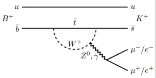
In QED the physical system consists of the electromagnetic field and (at least) one Dirac field. The system without interaction is described by the Hamiltonian $H_0=H_0^{\text {Dirac }}+H_0^{\text {em }}$ for the Dirac field and the electromagnetic field; the interaction between both fields is determined by the interaction Hamiltonian $$ H_{\mathrm{int}}=\int d^3 x \mathcal{H}{\text {int }}(x) $$ with a Hamiltonian density (conventionally denoted as Hamiltonian either) $$ \mathcal{H}{\text {int }}=e j^\mu A_\mu $$ involving the current $j^\mu$ of the Dirac field (see also Sec. $3.9$ and Sec. 4.4.5). The Hamiltonian of the entire system is thus given by $$ H=H_0+H_{\text {int }} . $$
物理代写|量子场论代写Quantum field theory代考|S-Matrix Elements and Feynman Graphs
For the matrix elements of the $S$-operator, the $S$-matrix elements, we introduce an abbreviated notation, $$ S_{f i}=\langle f|S| i\rangle $$ The $S$-operator transforms the initial state $|i\rangle$ by time evolution into $S|i\rangle \equiv\left|i^{\prime}\right\rangle$. The probability that the state $|f\rangle$ is contained in $\left|i^{\prime}\right\rangle$ is given by $$ \left|\left\langle f \mid i^{\prime}\right\rangle\right|^2=|\langle f|S| i\rangle|^2=\left|S_{f i}\right|^2 . $$ The calculation of the matrix elements for given particle processes is thus of crucial importance for the prediction of reaction rates and cross sections. The first-order approximation (3.51) for $S$ yields $$ S_{f i}=-i \int d^4 x\left\langle f\left|\mathcal{H}_{\text {int }}(x)\right| i\right\rangle $$ under the assumption that initial and final states are not identical. For the calculation of $S$-matrix elements a systematic method exists to display the matrix elements by Feynman graphs built by a set of Feynman rules. This would require, however, a somewhat extensive excursion into the formalism of quantum field theory and shall not be done within this introductory course. Instead, the procedure will be elucidated by means of a concrete example from which the Feynman rules can be read off that allow to obtain the matrix elements by graphical methods in an illustrative and efficient way.
statistics-lab™ 为您的留学生涯保驾护航 在代写量子场论Quantum field theory方面已经树立了自己的口碑, 保证靠谱, 高质且原创的统计Statistics代写服务。我们的专家在代写量子场论Quantum field theory代写方面经验极为丰富,各种代写量子场论Quantum field theory相关的作业也就用不着说。
我们提供的量子场论Quantum field theory及其相关学科的代写,服务范围广, 其中包括但不限于:
Statistical Inference 统计推断
Statistical Computing 统计计算
Advanced Probability Theory 高等概率论
Advanced Mathematical Statistics 高等数理统计学
(Generalized) Linear Models 广义线性模型
Statistical Machine Learning 统计机器学习
Longitudinal Data Analysis 纵向数据分析
Foundations of Data Science 数据科学基础
物理代写|量子场论代写Quantum field theory代考|PHYS3101
物理代写|量子场论代写Quantum field theory代考|Interacting Electromagnetic Field
Now we address the situation of the inhomogeneous wave equation (3.1) with the electromangetic current $j^\mu \sim \bar{\psi} \gamma^\mu \psi$, which is formed by the fermions $e^{\pm}, \mu^{\pm}, \ldots$ with the respective Dirac fields, according to Eq. (2.55). From now on we make use of the notation $$ \square A^\mu=e \bar{\psi} \gamma^\mu \psi \equiv e j^\mu $$ displaying the charge $e$ as a coupling constant explicitly. The solution of this inhomogenous differential equation for a given boundary condition is found with the help of the appropriate Green function $D_{\mu \nu}$ as follows, $$ A_\mu(x)=e \int d^4 y D_{\mu \nu}(x-y) j^\nu(y) . $$ $D_{\mu \nu}$ solves the inhomogeneous wave equation for a pointlike source, $$ \square_{(x)} D_{\mu \nu}(x-y)=g_{\mu \nu} \delta^4(x-y) . $$ Performing a Fourier transformation and using the formulae $$ \begin{aligned} \delta^4(x-y) & =\int \frac{d^4 Q}{(2 \pi)^4} e^{-i Q(x-y)}, \ D_{\mu \nu}(x-y) & =\int \frac{d^4 Q}{(2 \pi)^4} e^{-i Q(x-y)} D_{\mu \nu}(Q) \end{aligned} $$ one obtains an algebraic equation for the Fourier transformed $D_{\mu \nu}(Q)$, $$ -Q^2 D_{\mu \nu}(Q)=g_{\mu \nu} $$
物理代写|量子场论代写Quantum field theory代考|Interacting Dirac-Field
In Sec. $2.4$ the interaction of charged Dirac particles with an external electromagnetic field described by a classical vector potential was addressed. Now the complete interaction with the quantized electromagnetic field $A^\mu(x)$ is taken into account. For a given fermion species, for example electron/positron, with the respective Dirac field $\psi(x)$, the Dirac equation including the electromagnetic interaction follows fom the free Dirac equation (2.50) by means of the minimal substitution $i \partial_\mu \rightarrow i \partial_\mu-e A_\mu$, yielding $$ \left(i \gamma^\mu \partial_\mu-m\right) \psi=e \gamma^\mu A_\mu \psi $$ Treating the right-hand side as an inhomogeneity, a formal solution can specified by the method of Green functions, $$ \psi(x)=e \int d^4 y S(x-y) \gamma^\mu A_\mu(y) \psi(y) $$ Actually this formal “solution” is an integral equation for $\psi$; it is equivalent to the differential equation (3.32) together with a given boundary condition. The Green function $S(x-y)$ of the Dirac equation is a $4 \times 4$-matrix, defined as a solution of the Dirac equation for a pointline inhomogeneity, $$ \left(i \gamma^\mu \partial_\mu-m\right) S(x-y)=\mathbf{1} \delta^4(x-y) . $$ In analogy to the vector field one proceeds with the Fourier ansatz $$ S(x-y)=\int \frac{d^4 Q}{(2 \pi)^4} e^{-i Q(x-y)} S(Q) $$ converting Eq. (3.34) into an algebraic equation for $S(Q)$ in momentum space, $$ (\not-m) S(Q)=\mathbf{1} $$ with the solution
statistics-lab™ 为您的留学生涯保驾护航 在代写量子场论Quantum field theory方面已经树立了自己的口碑, 保证靠谱, 高质且原创的统计Statistics代写服务。我们的专家在代写量子场论Quantum field theory代写方面经验极为丰富,各种代写量子场论Quantum field theory相关的作业也就用不着说。
我们提供的量子场论Quantum field theory及其相关学科的代写,服务范围广, 其中包括但不限于:
Statistical Inference 统计推断
Statistical Computing 统计计算
Advanced Probability Theory 高等概率论
Advanced Mathematical Statistics 高等数理统计学
(Generalized) Linear Models 广义线性模型
Statistical Machine Learning 统计机器学习
Longitudinal Data Analysis 纵向数据分析
Foundations of Data Science 数据科学基础
物理代写|量子场论代写Quantum field theory代考|PHYSICS3544
物理代写|量子场论代写Quantum field theory代考|Quantized electromagnetic field
The quantized electromagnetic radiation field $A^\mu(x)$ represents the photon field, it is a field operator acting on the space of states of photons. Photons are particles with mass 0 and spin 1 ; the 4 -momentum $k^\mu$ thus fulfills the energy-momentum relation of a massless particle, $$ \left(k^0\right)^2-\vec{k}^2=0, \quad k^0=|\vec{k}| . $$ The space of states is constructed, in analogy to Klein-Gordon and Dirac particles, from the vacuum and the 1-particle states with momentum $k^\mu$ and helicity $\lambda=\pm 1$, vacuum (0-photon state) $\quad|0\rangle$ 1-photon states $\quad|k \lambda\rangle$ together with the two- and multi-particle states as symmetrized product states. The states are normalized according to $$ \langle 0 \mid 0\rangle=1, \quad\left\langle k \lambda \mid k^{\prime} \lambda^{\prime}\right\rangle=2 k^0 \delta_{\lambda \lambda^{\prime}} \delta^3\left(\vec{k}-\vec{k}^{\prime}\right) $$ The coefficients of the Fourier expansion of the field operator $A^\mu$ in terms of plane waves turn into the annihilation operators $a_\lambda(k)$ and creation operators $a_\lambda^{\dagger}(k)$ of photons with momentum $k^\mu$ und helicity $\lambda$, $$ A^\mu(x)=\frac{1}{(2 \pi)^{3 / 2}} \int \frac{d^3 k}{2 k^0} \sum_\lambda\left[a_\lambda(k) \epsilon_\lambda^\mu e^{-i k x}+a_\lambda^{\dagger}(k) \epsilon_\lambda^{\mu *} e^{i k x}\right] . $$ Since for photons particles and antiparticles are the same, there is only one species of annihilation and creation operators acting on the photon states as follows, $$ \begin{aligned} a_\lambda^{\dagger}(k)|0\rangle & =|k \lambda\rangle, \ a_\lambda(k)\left|k^{\prime} \lambda^{\prime}\right\rangle & =2 k^0 \delta^3\left(\vec{k}-\vec{k}^{\prime}\right) \delta_{\lambda \lambda^{\prime}}|0\rangle \end{aligned} $$ Being bosonic operators, $a_\lambda$ und $a_\lambda^{\dagger}$ fulfill canonical commutation rules like those for the scalar field, but with an additional spin index: $$ \left[a_\lambda(k), a_{\lambda^{\prime}}^{\dagger}\left(k^{\prime}\right)\right]=2 k^0 \delta^3\left(\vec{k}-\vec{k}^{\prime}\right) \delta_{\lambda \lambda^{\prime}}, \quad\left[a_\lambda(k), a_{\lambda^{\prime}}\left(k^{\prime}\right)\right]=0 . $$ Wave functions of 1-photon states are the matrix elements $$ \left\langle 0\left|A^\mu(x)\right| k \lambda\right\rangle=\frac{1}{(2 \pi)^{3 / 2}} \epsilon_\lambda^\mu(k) e^{-i k x},\left\langle k \lambda\left|A^\mu(x)\right| 0\right\rangle=\frac{1}{(2 \pi)^{3 / 2}} \epsilon_\lambda^{\mu *}(k) e^{i k x} . $$ They are used in the description of processes where photons are annihilated (left) or created (right).
物理代写|量子场论代写Quantum field theory代考|Mechanical observables
In correspondence to classical electrodynamics, Hamiltonian and momentum of the electromagnetic field are represented as integrals over the energy density and the momentum density in terms of the field operator, $$ \begin{aligned} H & =\frac{1}{2} \int d^3 x\left(\vec{E}^2+\vec{B}^2\right), \ \vec{P} & =\int d^3 x \vec{E} \times \vec{B} \end{aligned} $$ (see also Sec. 4.2.1). For the free radiation field in the radiation gauge (3.2) the field strengths are given by $$ \vec{E}=-\partial_0 \vec{A}, \quad \vec{B}=\nabla \times \vec{A} $$ Inserting the Fourier expansion (3.9) for $\vec{A}$ yields the instructive representation $$ \begin{aligned} & H=\int \frac{d^3 k}{2 k^0} \sum_\lambda k^0 N_\lambda(k), \ & \vec{P}=\int \frac{d^3 k}{2 k^0} \sum_\lambda \vec{k} N_\lambda(k) \end{aligned} $$ in terms of the number operators $N_\lambda(k)=a_\lambda^{\dagger}(k) a_\lambda(k)$ for photons. Using the relations $(3.10)$ it can easily be seen that the photon states $|p \sigma\rangle$ are eigenstates of $H$ and $\vec{P}$, $$ H|p \sigma\rangle=p^0|p \sigma\rangle, \quad \vec{P}|p \sigma\rangle=\vec{p}|p \sigma\rangle \text {. } $$ For photons as spin-1 particles the spin operator deserves an extra discussion. The spin operator for the radiation field is given by the expression $$ \vec{S}=\int d^3 x\left(i \partial_0 A_k\right)(\overrightarrow{\mathcal{S}})_l^k A^l $$ with the matrices $\overrightarrow{\mathcal{S}}=\left(\mathcal{S}^1, \mathcal{S}^2, \mathcal{S}^3\right)$ which are the generators of the 3-dimensional rotation group (see Sec. $4.2 .2$ for more details). For photons with momentum $p$ the helicity is defined, like for Dirac particles, as the projection of the spin on the momentum direction, $$ \vec{S} \cdot \frac{\vec{p}}{|\vec{p}|}=\vec{S} \cdot \vec{n}=\int d^3 x\left(i \partial_0 A_k\right)(\overrightarrow{\mathcal{S}} \cdot \vec{n})_l^k A^l $$
statistics-lab™ 为您的留学生涯保驾护航 在代写量子场论Quantum field theory方面已经树立了自己的口碑, 保证靠谱, 高质且原创的统计Statistics代写服务。我们的专家在代写量子场论Quantum field theory代写方面经验极为丰富,各种代写量子场论Quantum field theory相关的作业也就用不着说。
我们提供的量子场论Quantum field theory及其相关学科的代写,服务范围广, 其中包括但不限于:
Statistical Inference 统计推断
Statistical Computing 统计计算
Advanced Probability Theory 高等概率论
Advanced Mathematical Statistics 高等数理统计学
(Generalized) Linear Models 广义线性模型
Statistical Machine Learning 统计机器学习
Longitudinal Data Analysis 纵向数据分析
Foundations of Data Science 数据科学基础
物理代写|量子场论代写Quantum field theory代考|PHYS7076
物理代写|量子场论代写Quantum field theory代考|Covariant equation of motion
The correct relativistic version of Newton’s equation of motion can be formulated in terms of the 4-momentum and the proper time as follows, $$ \frac{d p^\mu}{d \tau}=K^\mu . $$ The quantity $K^\mu$ is a 4-vector, denoted as 4-force. Since all terms transform with the same matrix $\Lambda$, a Lorentz transformation into another reference frame, with $p^\mu \rightarrow p^{\prime \mu}, K^\mu \rightarrow K^{\prime \mu}$, yields the transformed equation of motion $$ \frac{d p^{\prime \mu}}{d \tau}=K^{\prime \mu} . $$ The individual components have changed, but the equation has the same form in different inertial frames; the equation is invariant in form, or covariant. In this context, covariant means that an equation can be written so that both sides have the same, well-defined, transformation properties under Lorentz transformations. This is an example for describing a physical law with the help of vector or tensor components, making Lorentz symmetry manifest. The 3-dimensional part of Eq. (1.44) can be cast into the form $$ \frac{d p^k}{d t}=K^k \sqrt{1-\frac{\vec{v}^2}{c^2}} \equiv F^k, $$ involving the 3 -dimensional force $\vec{F}$; an example will be given below. The physical meaning of the 0-component of the 4 -force follows from the indentity $$ p_\mu \frac{d p^\mu}{d \tau}=\frac{1}{2} \frac{d p^2}{d \tau}=0 \quad\left(\text { since } p^2=m^2 c^2\right) $$ together with $$ p_\mu \frac{d p^\mu}{d \tau}=p_\mu K^\mu=p_0 K^0-\vec{p} \vec{K}=0 $$ to become $$ p_0 K^0=\vec{p} \vec{K} . $$
物理代写|量子场论代写Quantum field theory代考|Free particle
Consider the free motion of a particle with mass $m$, described by the coordinates $x_i$ and the velocities $\dot{x}_i=v_i$. The corresponding Lagrangian is given by $$ L=-m \sqrt{1-\vec{v}^2} . $$ The equations of motions follow as the Euler-Lagrange equations, $$ \frac{d}{d t}\left(\frac{\partial L}{\partial v_i}\right)-\frac{\partial L}{\partial x_i}=0 $$ yielding $$ \frac{d}{d t}\left(\frac{m v_i}{\sqrt{1-\vec{v}^2}}\right)=0, \quad \frac{d \vec{p}}{d t}=0 . $$ They coincide with Eq. (1.46) for $\vec{F}=0$ and confirm Eq. (1.51) as the correct relativistic version for the Lagrangian of a free particle.
Hamiltonian. The Hamiltonian $H$ is derived from the Lagrangian $L$ by means of a Legrendre transformation, $$ H=\sum_i p_i v_i-L $$ with the canonical momenta $$ p_i=\frac{\partial L}{\partial v_i}, $$ where the velocities $v_i$ have to be substituted by the momenta $p_i$.
statistics-lab™ 为您的留学生涯保驾护航 在代写量子场论Quantum field theory方面已经树立了自己的口碑, 保证靠谱, 高质且原创的统计Statistics代写服务。我们的专家在代写量子场论Quantum field theory代写方面经验极为丰富,各种代写量子场论Quantum field theory相关的作业也就用不着说。
我们提供的量子场论Quantum field theory及其相关学科的代写,服务范围广, 其中包括但不限于:
Statistical Inference 统计推断
Statistical Computing 统计计算
Advanced Probability Theory 高等概率论
Advanced Mathematical Statistics 高等数理统计学
(Generalized) Linear Models 广义线性模型
Statistical Machine Learning 统计机器学习
Longitudinal Data Analysis 纵向数据分析
Foundations of Data Science 数据科学基础
物理代写|量子场论代写Quantum field theory代考|PHYS3101
物理代写|量子场论代写Quantum field theory代考|Lorentz Transformations
A Lorentz transformation from an inertial frame $K$ into another inertial frame $K^{\prime}$ is described by a linear transformation of the components $x^\mu$ in $K$ to $x^{\prime \mu}$ in $K^{\prime}$ with the help of a matrix $\Lambda=\left(\Lambda_\nu^\mu\right)$, $$ x^{\prime \mu}=\Lambda_\nu^\mu x^\nu \text {. } $$ The invariance of light propagation (1.1) is equivalent to the invariance of the scalar product under Lorentz transformations, which can be fomulated as a condition $$ g_{\rho \sigma} x^\rho x^\sigma=g_{\mu \nu} x^{\prime \mu} x^{\prime \nu}=g_{\mu \nu} \Lambda_\rho^\mu \Lambda_\sigma^\nu x^\rho x^\sigma $$ to be fulfilled for all $x^\mu$. Hence, Eq. (1.11) is a condition for the entries of $\Lambda$, $$ g_{\mu \nu} \Lambda_\rho^\mu \Lambda_\sigma^\nu=g_{\rho \sigma}, $$ or expressed in a compact way using the matrix $g=\left(g_{\mu \nu}\right)$ as follows, $$ \Lambda^T g \Lambda=g . $$ Applying the rules for determinants, $$ \operatorname{det}\left(\Lambda^T g \Lambda\right)=\operatorname{det}\left(\Lambda^T\right) \operatorname{det}(g) \operatorname{det}(\Lambda)=\operatorname{det}(g), $$ it immediately follows for the determinant of a Lorentz transformation that $$ \operatorname{det}(\Lambda)=\pm 1 . $$ As a consequence, the 4-dimensional volume element is invariant under Lorentz transformations, $$ \mathrm{d}^4 x=\mathrm{d} x^0 \mathrm{~d}^3 x \quad \rightarrow \quad \mathrm{d}^4 x^{\prime}=|\operatorname{det}(\Lambda)| \mathrm{d}^4 x=\mathrm{d}^4 x, $$ because $\Lambda$ is the Jacobian matrix of the transformation of variables $x^\mu \rightarrow x^{\prime \mu}$
物理代写|量子场论代写Quantum field theory代考|Mechanics
The motion of a particle with mass $m$ along a given trajectory is described by a time-dependent 3-dimensional vector $\vec{x}(t)$, with components $x^k(t)$, $k=1,2,3$. The velocity is as usual defined as the derivative $$ \vec{v}=\frac{d \vec{x}}{d t}=\left(v^1, v^2, v^3\right), \quad v^k=\frac{d x^k}{d t} . $$ The 4-dimensional trajectory is described by a curve in Minkowski space, $$ t \rightarrow x^\mu(t) \text { with } x^0(t)=c t, $$ denoted as the world line of the particle. For neighbouring points $x^\mu$ und $x^\mu+d x^\mu$ along the world line the difference is given by $$ d x^\mu=\frac{d x^\mu}{d t} d t $$ yielding the invariant 4-dimensional square, the line element of the world line, $$ \begin{aligned} d s^2 &=g_{\mu \nu} d x^\mu d x^\nu=g_{\mu \nu} \frac{d x^\mu}{d t} \frac{d x^\nu}{d t} d t^2 \ &=\left[\left(\frac{d x^0}{d t}\right)^2-\vec{v}^2\right] d t^2=c^2 d t^2\left[1-\frac{\vec{v}^2}{c^2}\right] \equiv c^2 d \tau^2 \end{aligned} $$
By this relation the invariant interval of the proper time is defined, $$ d \tau=d t \sqrt{1-\frac{\vec{v}^2}{c^2}} . $$ It is displayed by a co-moving clock.
statistics-lab™ 为您的留学生涯保驾护航 在代写量子场论Quantum field theory方面已经树立了自己的口碑, 保证靠谱, 高质且原创的统计Statistics代写服务。我们的专家在代写量子场论Quantum field theory代写方面经验极为丰富,各种代写量子场论Quantum field theory相关的作业也就用不着说。
我们提供的量子场论Quantum field theory及其相关学科的代写,服务范围广, 其中包括但不限于:
Statistical Inference 统计推断
Statistical Computing 统计计算
Advanced Probability Theory 高等概率论
Advanced Mathematical Statistics 高等数理统计学
(Generalized) Linear Models 广义线性模型
Statistical Machine Learning 统计机器学习
Longitudinal Data Analysis 纵向数据分析
Foundations of Data Science 数据科学基础
物理代写|量子场论代写Quantum field theory代考|PHYSICS3544
物理代写|量子场论代写Quantum field theory代考|Special Relativity
It is a assumed that the reader is already familiar with special relativity, e.g. at the level of a first course on electrodynamics. Thus, this chapter serves essentially as a summary of the relevant theoretical ingredients, to introduce notations and conventions, and to provide the classical basis for advancing to quantum theory in the subseqent chapters.
The Special Theory of Relativity is based on the following two fundamental principles. (1) Principle of relativity The laws of nature are in all inertial frames of the same form. (2) Invariance of light propagation The propagation of light is independent of the inertial frame. For a pointlike source at a space point $\vec{x}0$ and time $t_0$ in a given frame $K$ the outgoing lightfronts are spherical surfaces in all inertial frames, and propagate with $c$, the constant velocity of light, $$ \underbrace{c^2\left(t-t_0\right)^2-\left(\vec{x}-\vec{x}_0\right)^2}{\text {inertial frame } K}=0=\underbrace{c^2\left(t^{\prime}-t_0^{\prime}\right)^2-\left(\vec{x}^{\prime}-\vec{x}0^{\prime}\right)^2}{\text {inertial frame } K^{\prime}} . $$ Principle (2) is not valid for Galilei transformations between different frames. Thus, they have to be replaced by Lorentz transformations.
物理代写|量子场论代写Quantum field theory代考|Notations and Conventions
In a given inertial frame a space-time event is determined by a set of coordinates specifying the point $\vec{x}$ in space and $t$ in time. This information can be summarized by a four-component quantity $\left(x^\mu\right)$ according to $$ \left(x^\mu\right)=\left(x^0, x^1, x^2, x^3\right) \equiv\left(x^0, \vec{x}\right) $$ with $$ x^0=c t, \quad \vec{x}=\left(x^1, x^2, x^3\right) . $$ The $\left(x^\mu\right)$ form a 4-dimensional linear space, with elements denoted as 4-vectors and labeled by the symbol $x \equiv\left(x^\mu\right)$ as a short-hand notation. The quantities $x^\mu$ are called contravariant components. Convention: greek indices $\mu, \nu, \ldots=0,1,2,3$ latin indices $k, l, \ldots=1,2,3$. Metric. For the space of 4-vectors a scalar product is defined as a symmetric bilinear form as follows, $$ (x, y) \rightarrow x \cdot y=x^0 y^0-\vec{x} \cdot \vec{y}=g_{\mu \nu} x^\mu y^\nu $$ with the metric tensor $$ \left(g_{\mu \nu}\right)=\left(\begin{array}{cccc} 1 & 0 & 0 & 0 \ 0 & -1 & 0 & 0 \ 0 & 0 & -1 & 0 \ 0 & 0 & 0 & -1 \end{array}\right) $$ The square of a 4-vector is thus given by $$ x^2=x \cdot x=g_{\mu \nu} x^\mu x^\nu=\left(x^0\right)^2-\vec{x}^2 . $$ The 4-dimensional space of the $\left(x^\mu\right)$ with this metric is denoted as Minkowski space, the metric (1.4) as Minkowski metric.
statistics-lab™ 为您的留学生涯保驾护航 在代写量子场论Quantum field theory方面已经树立了自己的口碑, 保证靠谱, 高质且原创的统计Statistics代写服务。我们的专家在代写量子场论Quantum field theory代写方面经验极为丰富,各种代写量子场论Quantum field theory相关的作业也就用不着说。
我们提供的量子场论Quantum field theory及其相关学科的代写,服务范围广, 其中包括但不限于:
Statistical Inference 统计推断
Statistical Computing 统计计算
Advanced Probability Theory 高等概率论
Advanced Mathematical Statistics 高等数理统计学
(Generalized) Linear Models 广义线性模型
Statistical Machine Learning 统计机器学习
Longitudinal Data Analysis 纵向数据分析
Foundations of Data Science 数据科学基础
物理代写|量子场论代写Quantum field theory代考|PHYS8302
物理代写|量子场论代写Quantum field theory代考|Thermal Correlation Functions
The energies of excited states are encoded in the thermal correlation functions. These functions are expectation values of products of the position operator $$ \hat{q}{\mathrm{E}}(\tau)=\mathrm{e}^{\tau \hat{H} / \hbar} \hat{q} \mathrm{e}^{-\tau \hat{H} / \hbar}, \quad \hat{q}{\mathrm{E}}(0)=\hat{q}(0), $$ at different imaginary times in the canonical ensemble, $$ \left\langle\hat{q}{\mathrm{E}}\left(\tau{1}\right) \cdots \hat{q}{\mathrm{E}}\left(\tau{n}\right)\right\rangle_{\beta} \equiv \frac{1}{Z(\beta)} \operatorname{tr}\left(\mathrm{e}^{-\beta \hat{H}} \hat{q}{\mathrm{E}}\left(\tau{1}\right) \cdots \hat{q}{\mathrm{E}}\left(\tau{n}\right)\right) $$ The normalizing function $Z(\beta)$ is the partition function (2.56). From the thermal two-point function $$ \begin{aligned} \left\langle\hat{q}{\mathrm{E}}\left(\tau{1}\right) \hat{q}{\mathrm{E}}\left(\tau{2}\right)\right\rangle_{\beta} &=\frac{1}{Z(\beta)} \operatorname{tr}\left(\mathrm{e}^{-\beta \hat{H}} \hat{q}{\mathrm{E}}\left(\tau{1}\right) \hat{q}{\mathrm{E}}\left(\tau{2}\right)\right) \ &=\frac{1}{Z(\beta)} \operatorname{tr}\left(\mathrm{e}^{-\left(\beta-\tau_{1}\right) \hat{H}} \hat{q} \mathrm{e}^{-\left(\tau_{1}-\tau_{2}\right) \hat{H}} \hat{q} \mathrm{e}^{-\tau_{2} \hat{H}}\right) \end{aligned} $$ we can extract the energy gap between the ground state and the first excited state. For this purpose we use orthonormal energy eigenstates $|n\rangle$ to calculate the trace and in addition insert the resolution of the identity operator $\mathbb{1}=\sum|m\rangle\langle m|$. This yields $$ \langle\ldots\rangle_{\beta}=\frac{1}{Z(\beta)} \sum_{n, m} \mathrm{e}^{-\left(\beta-\tau_{1}+\tau_{2}\right) E_{n}} \mathrm{e}^{-\left(\tau_{1}-\tau_{2}\right) E_{\mathrm{m}}}\langle n|\hat{q}| m\rangle\langle m|\hat{q}| n\rangle $$ Note that in the sum over $n$ the contributions from the excited states are exponentially suppressed at low temperatures $\beta \rightarrow \infty$, implying that the thermal two-point function converges to the Schwinger function in this limit: $$ \left\langle\hat{q}{\mathrm{E}}\left(\tau{1}\right) \hat{q}{\mathrm{E}}\left(\tau{2}\right)\right\rangle_{\beta} \stackrel{\beta \rightarrow \infty}{\longrightarrow} \sum_{m>0} \mathrm{e}^{-\left(\tau_{1}-\tau_{2}\right)\left(E_{m}-E_{0}\right)}|\langle 0|\hat{q}| m\rangle|^{2}=\left\langle 0\left|\hat{q}{\mathrm{E}}\left(\tau{1}\right) \hat{q}{\mathrm{E}}\left(\tau{2}\right)\right| 0\right\rangle $$
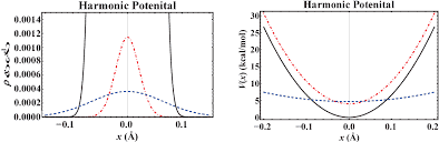
物理代写|量子场论代写Quantum field theory代考|The Harmonic Oscillator
We wish to study the path integral for the Euclidean oscillator with discretized time. The oscillator is one of the few systems for which the path integral can be calculated explicitly. For more such system, the reader may consult the text [19]. But the results for the oscillator are particularly instructive with regard to lattice field theories considered later in this book. So let us discretize the Euclidean time interval $[0, \tau]$ with $n$ sampling points separated by a lattice constant $\varepsilon=\tau / n$. For the Lagrangian $$ L=\frac{m}{2} \dot{q}^{2}+\mu q^{2} $$ the discretized path integral over periodic paths reads $$ \begin{aligned} Z &=\int \mathrm{d} q_{1} \cdots \mathrm{d} q_{n}\left(\frac{m}{2 \pi \varepsilon}\right)^{n / 2} \exp \left{-\varepsilon \sum_{j=0}^{n-1}\left(\frac{m}{2}\left(\frac{q_{j+1}-q_{j}}{\varepsilon}\right)^{2}+\mu q_{j}^{2}\right)\right} \ &=\left(\frac{m}{2 \pi \varepsilon}\right)^{n / 2} \int \mathrm{d} q_{1} \cdots \mathrm{d} q_{n} \exp \left(-\frac{1}{2}(\boldsymbol{q}, \mathrm{A} q)\right) \end{aligned} $$ where we assumed $q_{0}=q_{n}$ and introduced the symmetric matrix $$ \mathrm{A}=\frac{m}{\varepsilon}\left(\begin{array}{cccccc} \alpha & -1 & 0 & \cdots & 0 & -1 \ -1 & \alpha & -1 & \cdots & 0 & 0 \ & & \ddots & & & \ & & & \ddots & & \ 0 & 0 & \cdots & -1 & \alpha & -1 \ -1 & 0 & \cdots & 0 & -1 & \alpha \end{array}\right), \quad \alpha=2\left(1+\frac{\mu}{m} \varepsilon^{2}\right) $$ This is a Toeplitz matrix in which each descending diagonal from left to right is constant. This property results from the invariance of the action under lattice translations. For the explicit calculation of $Z$, we consider the generating function $$ \begin{aligned} Z[j] &=\left(\frac{m}{2 \pi \varepsilon}\right)^{n / 2} \int \mathrm{d}^{n} q \exp \left{-\frac{1}{2}(\boldsymbol{q}, \mathrm{A} q)+(\boldsymbol{j}, \boldsymbol{q})\right} \ &=\frac{(m / \varepsilon)^{n / 2}}{\sqrt{\operatorname{det} \mathrm{A}}} \exp \left{\frac{1}{2}\left(j, \mathrm{~A}^{-1} \boldsymbol{j}\right)\right} \end{aligned} $$
物理代写|量子场论代写Quantum field theory代考|Problems
2.1 (Gaussian Integral) Show that $$ \int \mathrm{d} z_{1} \mathrm{~d} \bar{z}{1} \ldots \mathrm{d} z{n} \mathrm{~d} \bar{z}{n} \exp \left(-\sum{i j} \bar{z}{i} A{i j} z_{j}\right)=\pi^{n}(\operatorname{det} \mathrm{A})^{-1} $$ with A being a positive Hermitian $n \times n$ matrix and $z_{i}$ complex integration variables. 2.2 (Harmonic Oscillator) In (2.43) we quoted the result for the kernel $K_{\omega}\left(\tau, q^{\prime}, q\right)$ of the $d$-dimensional harmonic oscillator with Hamiltonian $$ \hat{H}=\frac{1}{2 m} \hat{p}^{2}+\frac{m \omega^{2}}{2} \hat{q}^{2} $$ at imaginary time $\tau$. Derive this formula. Hint: Express the kernel in terms of the eigenfunctions of $\hat{H}$, which for $\hbar=m=$ $\omega=1$ are given by $$ \exp \left(-\xi^{2}-\eta^{2}\right) \sum_{n=0}^{\infty} \frac{\alpha^{n}}{2^{n} n !} H_{n}(\xi) H_{n}(\eta)=\frac{1}{\sqrt{1-\alpha^{2}}} \exp \left(\frac{-\left(\xi^{2}+\eta^{2}-2 \xi \eta \alpha\right)}{1-\alpha^{2}}\right) $$ The functions $H_{n}$ denote the Hermite polynomials. Comment: This result also follows from the direct evaluation of the path integral. 2.3 (Free Particle on a Circle) A free particle moves on an interval and obeys periodic boundary conditions. Compute the time evolution kernel $K\left(t_{b}-t_{a}, q_{b}, q_{a}\right)=$ $\left\langle q_{b}, t_{b} \mid q_{a}, t_{a}\right\rangle$. Use the familiar formula for the kernel of the free particle (2.26) and enforce the periodic boundary conditions by a suitable sum over the evolution kernel for the particle on $\mathbb{R}$.
statistics-lab™ 为您的留学生涯保驾护航 在代写量子场论Quantum field theory方面已经树立了自己的口碑, 保证靠谱, 高质且原创的统计Statistics代写服务。我们的专家在代写量子场论Quantum field theory代写方面经验极为丰富,各种代写量子场论Quantum field theory相关的作业也就用不着说。
我们提供的量子场论Quantum field theory及其相关学科的代写,服务范围广, 其中包括但不限于:
Statistical Inference 统计推断
Statistical Computing 统计计算
Advanced Probability Theory 高等概率论
Advanced Mathematical Statistics 高等数理统计学
(Generalized) Linear Models 广义线性模型
Statistical Machine Learning 统计机器学习
Longitudinal Data Analysis 纵向数据分析
Foundations of Data Science 数据科学基础
物理代写|量子场论代写Quantum field theory代考|PHYS3101
物理代写|量子场论代写Quantum field theory代考|Quantum Mechanics in Imaginary Time
The unitary time evolution operator has the spectral representation $$ \hat{K}(t)=\mathrm{e}^{-\mathrm{i} \hat{H} t}=\int \mathrm{e}^{-\mathrm{i} E t} \mathrm{~d} \hat{P}{\mathrm{E}}, $$ where $\hat{P}{\mathrm{E}}$ is the spectral family of the Hamiltonian. If $\hat{H}$ has discrete spectrum, then $\hat{P}{\mathrm{E}}$ is the orthogonal projector onto the subspace of $\mathscr{H}$ spanned by all eigenfunctions with energies less than $E$. In the following we assume that the Hamiltonian operator is bounded from below. Then we can subtract its ground state energy to obtain a non-negative $\hat{H}$ for which the integration limits in (2.35) are 0 and $\infty$. With the substitution $t \rightarrow t-\mathrm{i} \tau$, we obtain $$ \mathrm{e}^{-(\tau+\mathrm{i} t) \hat{H}}=\int{0}^{\infty} \mathrm{e}^{-E(\tau+\mathrm{i} t)} \mathrm{d} \hat{P}_{\mathrm{E}} $$ This defines a holomorphic semigroup in the lower complex half-plane $$ {z=t-\mathrm{i} \tau \in \mathbb{C}, \tau \geq 0} $$ If the operator $(2.36)$ is known on the negative imaginary axis $(t=0, \tau \geq 0)$, one can perform an analytic continuation to the real axis $(t, \tau=0)$. The analytic continuation to complex time $t \rightarrow-\mathrm{i} \tau$ corresponds to a transition from the Minkowski metric $\mathrm{d} s^{2}=d t^{2}-\mathrm{d} x^{2}-\mathrm{d} y^{2}-\mathrm{d} z^{2}$ to a metric with Euclidean signature. Hence a theory with imaginary time is called Euclidean theory.
The time evolution operator $\hat{K}(t)$ exists for real time and defines a oneparametric unitary group. It fulfills the Schrödinger equation $$ \mathrm{i} \frac{\mathrm{d}}{\mathrm{d} t} \hat{K}(t)=\hat{H} \hat{K}(t) $$ with a complex and oscillating kernel $K\left(t, q^{\prime}, q\right)=\left\langle q^{\prime}|\hat{K}(t)| q\right\rangle$. For imaginary time we have a Hermitian (and not unitary) evolution operator $$ \hat{K}(\tau)=\mathrm{e}^{-\tau \hat{H}} $$ with positive spectrum. The $\hat{K}(\tau)$ exist for positive $\tau$ and form a semi-group only. For almost all initial data, evolution back into the “imaginary past” is impossible. The evolution operator for imaginary time satisfies the heat equation $$ \frac{\mathrm{d}}{\mathrm{d} \tau} \hat{K}(\tau)=-\hat{H} \hat{K}(\tau) $$ instead of the Schrödinger equation and has kernel $$ K\left(\tau, q^{\prime}, q\right)=\left\langle q^{\prime}\left|\mathrm{e}^{-\tau \hat{H}}\right| q\right\rangle, \quad K\left(0, q^{\prime}, q\right)=\delta\left(q^{\prime}, q\right) $$ This kernel is real ${ }^{1}$ for a real Hamiltonian. Furthermore it is strictly positive:
物理代写|量子场论代写Quantum field theory代考|Imaginary Time Path Integral
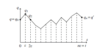
To formulate the path integral for imaginary time, we employ the product formula $(2.28)$, which follows from the product formula (2.27) through the substitution of it by $\tau$. For such systems the analog of $(2.31)$ for Euclidean time $\tau$ is obtained by the substitution of $i \varepsilon$ by $\varepsilon$. Thus we tind $$ \begin{aligned} K\left(\tau, q^{\prime}, q\right) &=\left\langle\hat{q}^{\prime}\left|\mathrm{e}^{-\tau \hat{H} / \hbar}\right| \hat{q}\right\rangle \ &=\lim {n \rightarrow \infty} \int \mathrm{d} q{1} \cdots \mathrm{d} q_{n-1}\left(\frac{m}{2 \pi \hbar \varepsilon}\right)^{n / 2} \mathrm{e}^{-S_{\mathrm{E}}\left(q_{0}, q_{1}, \ldots, q_{n}\right) / \hbar} \ S_{\mathrm{E}}(\ldots) &=\varepsilon \sum_{j=0}^{n-1}\left{\frac{m}{2}\left(\frac{q_{j+1}-q_{j}}{\varepsilon}\right)^{2}+V\left(q_{j}\right)\right} \end{aligned} $$ where $q_{0}=q$ and $q_{n}=q^{\prime}$. The multidimensional integral represents the sum over all broken-line paths from $q$ to $q^{\prime}$. Interpreting $S_{\mathrm{E}}$ as Hamiltonian of a classical lattice model and $\hbar$ as temperature, it is (up to the fixed endpoints) the partition function of a one-dimensional lattice model on a lattice with $n+1$ sites. The realvalued variable $q_{j}$ defined on site $j$ enters the action $S_{\mathrm{E}}$ which contains interactions between the variables $q_{j}$ and $q_{j+1}$ at neighboring sites. The values of the lattice field $$ {0,1, \ldots, n-1, n} \rightarrow\left{q_{0}, q_{1}, \ldots, q_{n-1}, q_{n}\right} $$ are prescribed at the endpoints $q_{0}=q$ and $q_{n}=q^{\prime}$. Note that the classical limit $\hbar \rightarrow 0$ corresponds to the low-temperature limit of the lattice system.
The multidimensional integral (2.52) corresponds to the summation over all path on the time lattice. What happens to the finite-dimensional integral when we take the continuum limit $n \rightarrow \infty$ ? Then we obtain the Euclidean path integral representation for the positive kernel $$ K\left(\tau, q^{\prime}, q\right)=\left\langle q^{\prime}\left|\mathrm{e}^{-\tau \hat{H} / h}\right| q\right\rangle=C \int_{q(0)=q}^{q(\tau)=q^{\prime}} \mathscr{D} q \mathrm{e}^{-S_{\mathrm{E}}[q] / h} $$ The integrand contains the Euclidean action $$ S_{\mathrm{E}}[q]=\int_{0}^{\tau} d \sigma\left{\frac{m}{2} \dot{q}^{2}+V(q(\sigma))\right} $$ which for many physical systems is bounded from below.
物理代写|量子场论代写Quantum field theory代考|Path Integral in Quantum Statistics
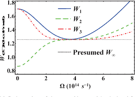
The Euclidean path integral formulation immediately leads to an interesting connection between quantum statistical mechanics and classical statistical physics. Indeed, if we set $\tau / \hbar \equiv \beta$ and integrate over $q=q^{\prime}$ in (2.53), then we end up with the path integral representation for the canonical partition function of a quantum system with Hamiltonian $\hat{H}$ at inverse temperature $\beta=1 / k_{B} T$. More precisely, setting $q=q^{\prime}$ and $\tau=\hbar \beta$ in the left-hand side of this formula, then the integral over $q$ yields the trace of $\exp (-\beta \hat{H})$, which is just the canonical partition function, $$ \int \mathrm{d} q K(\hbar \beta, q, q)=\operatorname{tr} \mathrm{e}^{-\beta \hat{H}}=Z(\beta)=\sum \mathrm{e}^{-\beta E_{n}} \quad \text { with } \quad \beta=\frac{1}{k_{B} T} $$ Setting $q=q^{\prime}$ in the Euclidean path integral in (2.53) means that we integrate over paths beginning and ending at $q$ during the imaginary time interval $[0, \hbar \beta]$. The final integral over $q$ leads to the path integral over all periodic paths with period $\hbar \beta$ $$ Z(\beta)=C \oint \mathscr{D} q \mathrm{e}^{-S_{\mathrm{E}}[q] / \hbar}, \quad q(\hbar \beta)=q(0) $$ For example, the kernell of the harmonic oscillator in $(2.43)$ on the diagonal is $$ K_{\omega}(\beta, q, q)=\sqrt{\frac{m \omega}{2 \pi \sinh (\omega \beta)}} \exp \left{-m \omega \tanh (\omega \beta / 2) q^{2}\right} $$ where we used units with $\hbar=1$. The integral over $q$ yields the partition function $$ \begin{aligned} Z(\beta) &=\sqrt{\frac{m \omega}{2 \pi \sinh (\omega \beta)}} \int \mathrm{d} q \exp \left{-m \omega \tanh (\omega \beta / 2) q^{2}\right} \ &=\frac{1}{2 \sinh (\omega \beta / 2)}=\frac{\mathrm{e}^{-\omega \beta / 2}}{1-\mathrm{e}^{-\omega \beta}}=\mathrm{e}^{-\omega \beta / 2} \sum_{n=0}^{\infty} \mathrm{e}^{-n \omega \beta} \end{aligned} $$ where we used $\sinh x=2 \sinh x / 2 \cosh x / 2$. A comparison with the spectral sum over all energies in (2.55) yields the energies of the oscillator with (angular) frequency $\omega$, $$ E_{n}=\omega\left(n+\frac{1}{2}\right), \quad n=0,1,2, \ldots $$ For large values of $\omega \beta$, i.e., for very low temperature, the spectral sum is dominated by the contribution of the ground state energy. Thus for cold systems, the free energy converges to the ground state energy $$ F(\beta) \equiv-\frac{1}{\beta} \log Z(\beta) \stackrel{\omega \beta \rightarrow \infty}{\longrightarrow} E_{0} $$ One often is interested in the energies and wave functions of excited states. We now discuss an elegant method to extract this information from the path integral.
S_{\mathrm{E}}[q]=\int_{0}^{\tau} d \sigma\left{\frac{m}{2} \dot{q}^{2}+V(q( \sigma))\对}S_{\mathrm{E}}[q]=\int_{0}^{\tau} d \sigma\left{\frac{m}{2} \dot{q}^{2}+V(q( \sigma))\对} 对于许多物理系统来说,它是从下面限定的。
物理代写|量子场论代写Quantum field theory代考|Path Integral in Quantum Statistics
statistics-lab™ 为您的留学生涯保驾护航 在代写量子场论Quantum field theory方面已经树立了自己的口碑, 保证靠谱, 高质且原创的统计Statistics代写服务。我们的专家在代写量子场论Quantum field theory代写方面经验极为丰富,各种代写量子场论Quantum field theory相关的作业也就用不着说。
我们提供的量子场论Quantum field theory及其相关学科的代写,服务范围广, 其中包括但不限于:
Statistical Inference 统计推断
Statistical Computing 统计计算
Advanced Probability Theory 高等概率论
Advanced Mathematical Statistics 高等数理统计学
(Generalized) Linear Models 广义线性模型
Statistical Machine Learning 统计机器学习
Longitudinal Data Analysis 纵向数据分析
Foundations of Data Science 数据科学基础
物理代写|量子场论代写Quantum field theory代考|PHYSICS 3544
物理代写|量子场论代写Quantum field theory代考|Path Integrals in Quantum and Statistical Mechanics
Already back in 1933 , Dirac asked himself whether the classical Lagrangian and action are as significant in quantum mechanics as they are in classical mechanics $[1,2]$. He observed that for simple systems, the probability amplitude $$ K\left(t, q^{\prime}, q\right)=\left\langle q^{\prime}\left|\mathrm{e}^{-\mathrm{i} \hat{A} t / h}\right| q\right\rangle $$ for the propagation from a point with coordinate $q$ to another point with coordinate $q^{\prime}$ in time $t$ is given by $$ K\left(t, q^{\prime}, q\right) \propto \mathrm{e}^{\mathrm{i} S\left[q_{\mathrm{cl}}\right] / h} $$ where $q_{\mathrm{cl}}$ denotes the classical trajectory from $q$ to $q^{\prime}$. In the exponent the action of this trajectory enters as a multiple of Planck’s reduced constant $h$. For a free particle with Lagrangian $$ L_{0}=\frac{m}{2} \dot{q}^{2} $$ the formula $(2.2)$ is verified easily: A free particle moves with constant velocity $\left(q^{\prime}-q\right) / t$ from $q$ to $q^{\prime}$ and the action of the classical trajectory is $$ S\left[q_{\mathrm{cl}}\right]=\int_{0}^{t} \mathrm{~d} s L_{0}\left[q_{\mathrm{cl}}(s)\right]=\frac{m}{2 t}\left(q^{\prime}-q\right)^{2} $$ The factor of proportionality in $(2.2)$ is then uniquely fixed by the condition $\mathrm{e}^{-\mathrm{i} \hat{H} t / \hbar} \longrightarrow 1$ for $t \rightarrow 0$ which in position space reads $$ \lim {t \rightarrow 0} K\left(t, q^{\prime}, q\right)=\delta\left(q^{\prime}, q\right) $$ Alternatively, it is fixed by the property $\mathrm{e}^{-\mathrm{i} \hat{H} t / h} \mathrm{e}^{-\mathrm{i} \hat{H} s / h}=\mathrm{e}^{-\mathrm{i} \hat{H}(t+s) / h}$ that takes the form $$ \int \mathrm{d} u K\left(t, q^{\prime}, u\right) K(s, u, q)=K\left(t+s, q^{\prime}, q\right) $$ in position space. Thus, the correct free particle propagator on a line is given by $$ K{0}\left(t, q^{\prime} \cdot q\right)=\left(\frac{m}{2 \pi \mathrm{i} \hbar t}\right)^{1 / 2} \mathrm{c}^{\mathrm{i} m\left(q^{\prime}-q\right)^{2} / 2 h t} $$ Similar results hold for the harmonic oscillator or systems for which $\langle\hat{q}(t)\rangle$ fulfills the classical equation of motion. For such systems $\left\langle V^{\prime}(\hat{q})\right\rangle=V^{\prime}(\langle\hat{q}\rangle)$ holds true. However, for general systems, the simple formula (2.2) must be extended, and it was Feynman who discovered this extension back in 1948. He realized that all paths from $q$ to $q^{\prime}$ (and not only the classical path) contribute to the propagator. This means that in quantum mechanics a particle can potentially move on any path $q(s)$ from the initial to the final destination, $$ q(0)=q \quad \text { and } \quad q(t)=q^{\prime} $$
物理代写|量子场论代写Quantum field theory代考|Recalling Quantum Mechanics
There are two well-established ways to quantize a classical system: canonical quantization and path integral quantization. For completeness and later use, we recall the main steps of canonical quantization both in Schrödinger’s wave mechanics and Heisenberg’s matrix mechanics.
A classical system is described by its coordinates $\left{q^{i}\right}$ and momenta $\left{p_{i}\right}$ on phase space $\Gamma$. An observable $O$ is a real-valued function on $\Gamma$. Examples are the coordinates on phase space and the energy $H(q, p)$. We assume that phase space comes along with a symplectic structure and has local coordinates with Poisson brackets $$ \left{q^{i}, p_{j}\right}=\delta_{j}^{i} $$ The brackets are extended to observables on through antisymmetry and the derivation rule ${O P, Q}=O{P, Q}+{O, Q} P$. The evolution in time of an observable is determined by $$ \dot{O}={O, H}, \quad \text { e.g. } \quad \dot{q}^{i}=\left{q^{i}, H\right} \quad \text { and } \quad \dot{p}{i}=\left{p{i}, H\right} $$ In the canonical quantization, functions on phase space are mapped to operators, and the Poisson brackets of two functions become commutators of the associated operators: $$ O(q, p) \rightarrow \hat{O}(\hat{q}, \hat{p}) \quad \text { and } \quad{O, P} \longrightarrow \frac{1}{\mathrm{i} \hbar}[\hat{O}, \hat{P}] $$
The time evolution of an (not explicitly time-dependent) observable is determined by Heisenberg’s equation $$ \frac{\mathrm{d} \hat{O}}{\mathrm{~d} t}=\frac{\mathrm{i}}{\hbar}[\hat{H}, \hat{O}] $$ In particular the phase space coordinates $\left(q^{l}, p_{i}\right)$ become operators with commutation relations $\left[\hat{q}^{i}, \hat{p}{j}\right]=\mathrm{i} \hbar \delta{j}^{i}$, and their time evolution is determined by $$ \frac{\mathrm{d} \hat{q}^{i}}{\mathrm{~d} t}=\frac{\mathrm{i}}{\hbar}\left[\hat{H}, \hat{q}^{i}\right] \quad \text { and } \quad \frac{\mathrm{d} \hat{p}{i}}{\mathrm{~d} t}=\frac{\mathrm{i}}{\hbar}\left[\hat{H}, \hat{p}{i}\right] $$ For a system of non-relativistic and spinless particles, the Hamiltonian reads $$ \hat{H}=\hat{H}{0}+\hat{V} \quad \text { with } \quad \hat{H}{0}=\frac{1}{2 m} \sum \hat{p}{i}^{2} $$ and one arrives at Heisenberg’s equations of motion $$ \frac{\mathrm{d} \hat{q}^{i}}{\mathrm{~d} t}=\frac{\hat{p}{i}}{m} \quad \text { and } \quad \frac{\mathrm{d} \hat{p}{i}}{\mathrm{~d} t}=-\hat{V}{, i} $$ Observables are represented by Hermitian operators on a Hilbert space $\mathscr{H}$, whose elements characterize the states of the system: $$ \hat{O}(\hat{q}, \hat{p}): \mathcal{H} \longrightarrow \mathcal{H} $$ Consider a particle confined to an endless wire. Its Hilbert space is $\mathcal{H}=L_{2}(\mathbb{R})$, and its position and momentum operator are represented in position space as $$ (\hat{q} \psi)(q)=q \psi(q) \quad \text { and } \quad(\hat{p} \psi)(q)=\frac{\hbar}{i} \partial_{q} \psi(q) $$
物理代写|量子场论代写Quantum field theory代考|Feynman–Kac Formula
We shall derive Feynman’s path integral representation for the unitary time evolution operator $\exp (-\mathrm{i} \hat{H} t)$ as well as Kac’s path integral representation for the positive operator $\exp (-\hat{H} \tau)$. Thereby we shall utilize the product formula of Trotter. In case of matrices, this formula was already verified by Lie and has the form: Theorem 2.1 (Lie’s Theorem) For two matrices $\mathrm{A}$ and $\mathrm{B}$ $$ \mathrm{e}^{\mathrm{A}+\mathrm{B}}=\lim {n \rightarrow \infty}\left(\mathrm{e}^{\mathrm{A} / n} \mathrm{e}^{\mathrm{B} / n}\right)^{n} $$ To prove this theorem, we define for each $n$ the two matrices $\mathrm{S}{n}:=\exp (\mathrm{A} / n+\mathrm{B} / n)$ and $\mathrm{T}{n}:=\exp (\mathrm{A} / n) \exp (\mathrm{B} / n)$ and telescope the difference of their $n$ ‘th powers, $$ \mathrm{S}{n}^{n}-\mathrm{T}{n}^{n}=\mathrm{S}{n}^{n-1}\left(\mathrm{~S}{n}-\mathrm{T}{n}\right)+\mathrm{S}{n}^{n-2}\left(\mathrm{~S}{n}-\mathrm{T}{n}\right) \mathrm{T}{n}+\cdots+\left(\mathrm{S}{n}-\mathrm{T}{n}\right) \mathrm{T}{n}^{n-1} $$ Now we choose any (sub-multiplicative) matrix norm, for example, the Frobenius norm. The triangle inequality together with $|X Y| \leq|X \mid| Y |$ imply the inequality $|\exp (X)| \leq \exp (|X|)$ such that $$ \left|\mathrm{S}{n}\right|,\left|\mathrm{T}{n}\right| \leq a^{1 / n} \quad \text { with } \quad a=\mathrm{e}^{|\mathrm{A}|+|\mathrm{B}|} $$ Thus we conclude $$ \left|\mathrm{S}{n}^{n}-\mathrm{T}{n}^{n}\right| \equiv\left|\mathrm{e}^{\mathrm{A}+B}-\left(\mathrm{e}^{\mathrm{A} / n} \mathrm{e}^{B / n}\right)^{n}\right| \leq n \times a^{(n-1) / n}\left|\mathrm{~S}{n}-\mathrm{T}{n}\right| $$ Finally, using $\mathrm{S}{n}-\mathrm{T}_{n}=-[\mathrm{A}, \mathrm{B}] / 2 n^{2}+O\left(1 / n^{3}\right)$, the product formula is verified for matrices. But the theorem also holds for self-adjoint operators.
Theorem $2.2$ (Trotter’s Theorem) If $\hat{A}$ and $\hat{B}$ are self-adjoint operators and $\hat{A}+$ $\hat{B}$ is essentially self-adjoint on the intersection $\mathscr{D}$ of their domains, then $$ \mathrm{e}^{-\mathrm{i} t(\hat{A}+\hat{B})}=s-\lim {n \rightarrow \infty}\left(\mathrm{e}^{-\mathrm{i} t \hat{A} / n} \mathrm{e}^{-\mathrm{i} t \hat{B} / n}\right)^{n} $$ If in addition $\hat{A}$ and $\hat{B}$ are bounded from below, then $$ \mathrm{e}^{-\tau(\hat{A}+\hat{B})}=s-\lim {n \rightarrow \infty}\left(\mathrm{e}^{-\tau \hat{A} / n} \mathrm{e}^{-\tau \hat{B} / n}\right)^{n} $$ The operators need not be bounded and the convergence is with respect to the strong operator topology. For operators $\hat{A}{n}$ and $\hat{A}$ on a common domain $\mathscr{D}$ in the Hilbert space, we have s- $\lim {n \rightarrow \infty} \hat{A}{n}=\hat{A}$ iff $\left|\hat{A}{n} \psi-\hat{A} \psi\right| \rightarrow 0$ for all $\psi \in \mathscr{D}$. Formula (2.27) is used in quantum mechanics, and formula $(2.28)$ finds its application in statistical physics and the Euclidean formulation of quantum mechanics [16].
Let us assume that $\hat{H}$ can be written as $\hat{H}=\hat{H}{0}+\hat{V}$ and apply the product formula to the evolution kernel in (2.22). With $\varepsilon=t / n$ and $\hbar=1$, we obtain $$ \begin{aligned} K\left(t, q^{\prime}, q\right) &=\lim {n \rightarrow \infty}\left\langle q^{\prime}\left|\left(\mathrm{e}^{-\mathrm{i} \varepsilon \hat{H}{0}} \mathrm{e}^{-\mathrm{i} \varepsilon \hat{V}}\right)^{n}\right| q\right\rangle \ &=\lim {n \rightarrow \infty} \int \mathrm{d} q_{1} \cdots \mathrm{d} q_{n-1} \prod_{j=0}^{j=n-1}\left|q_{j+1}\right| \mathrm{e}^{-\mathrm{i} \varepsilon \hat{H}{0}} \mathrm{e}^{-i \varepsilon \hat{V}}\left|q{j}\right\rangle \end{aligned} $$ where we repeatedly inserted the resolution of the identity $(2.21)$ and denoted the initial and final point by $q_{0}=q$ and $q_{n}=q^{\prime}$, respectively. The potential $\hat{V}$ is diagonal in position space such that $$ \left\langle q_{j+1}\left|\mathrm{e}^{-\mathrm{i} \varepsilon \hat{H}{0}} \mathrm{e}^{-\mathrm{i} \varepsilon \hat{V}}\right| q{j}\right\rangle=\left\langle q_{j+1}\left|\mathrm{e}^{-\mathrm{i} \varepsilon \hat{H}{0}}\right| q{j}\right\rangle \mathrm{e}^{-\mathrm{i} \varepsilon V\left(q_{j}\right)} $$
statistics-lab™ 为您的留学生涯保驾护航 在代写量子场论Quantum field theory方面已经树立了自己的口碑, 保证靠谱, 高质且原创的统计Statistics代写服务。我们的专家在代写量子场论Quantum field theory代写方面经验极为丰富,各种代写量子场论Quantum field theory相关的作业也就用不着说。
我们提供的量子场论Quantum field theory及其相关学科的代写,服务范围广, 其中包括但不限于:
Statistical Inference 统计推断
Statistical Computing 统计计算
Advanced Probability Theory 高等概率论
Advanced Mathematical Statistics 高等数理统计学
(Generalized) Linear Models 广义线性模型
Statistical Machine Learning 统计机器学习
Longitudinal Data Analysis 纵向数据分析
Foundations of Data Science 数据科学基础
物理代写|量子场论代写Quantum field theory代考|PHYS8302
物理代写|量子场论代写Quantum field theory代考|Symmetric Tensors
There is a very important twist to the notion of tensor product when one considers systems composed of several, say $n$ identical particles. Identical particles are indistinguishable from each other, even in principle. If an electron in motion scatters on an electron at rest, two moving electrons come out of the experiment and there is no way telling which of them was the electron at rest (and it can be argued that the question may not even make sense). This has to be built in the model. To this aim, we consider a Hilbert space $\mathcal{H}$ with a basis $\left(e_{i}\right){i \geq 1}$, a given integer $n$ and we denote by $\mathcal{H}{n}$ the tensor product of $n$ copies of it, in the above sense. We observe that a permutation $\sigma$ of ${1,2, \ldots, n}$ induces a transformation of $\mathcal{H}{n}$, simply by transforming the basis element $\bigotimes{k \leq n} e_{i_{k}}$ into $\bigotimes_{k \leq n} e_{i_{\sigma(k)}}$. If an element $x$ of $\mathcal{H}_{n}$ describes the state of a system consisting of $n$ identical particles, its image under this transformation describes the same particle system, so that it must be of the type $\lambda x$ for
$\lambda \in \mathbb{C}$. Since the transform of $x$ has the same norm as $x$ then $|\lambda|=1$, that is the transform of $x$ differs from $x$ only by a phase. 10
In Part I of this book we consider the simplest case where the transform of each state $x$ is $x$ itself. Particles with this property are called bosons. 11 These are not the most common and interesting particles, but must be understood first. Later on, we will meet fermions, which comprise most of the important particles (and in particular electrons). Let us denote by $\mathrm{S}_{n}$ the group of permutations of ${1, \ldots, n}$.
物理代写|量子场论代写Quantum field theory代考|Creation and Annihilation Operators
We define and study the operators $A_{n}(\xi)$ and $A_{n}^{\dagger}(\eta)$, which will play a crucial role in the next section. It is convenient here to define $\mathcal{H}{0, s}:=\mathbb{C}$. For $n \geq 1$ and $\xi \in \mathcal{H}$ the operator $A{n}(\xi): \mathcal{H}{n, s} \rightarrow \mathcal{H}{n-1, s}$ transforms an $n$-particle state into an $(n-1)$-particle state, and for this reason is called an annihilation operator. For $n \geq 0$ and $\eta \in \mathcal{H}$ the operator $A_{n}^{\dagger}(\eta)$ : $\mathcal{H}{n, s} \rightarrow \mathcal{H}{n+1, s}$ transforms an $n$-particle state into an $(n+1)$-particle state, and is called a creation operator.
In order to avoid writing formulas which are too abstract, we pick an orthonormal basis $\left(e_{i}\right){i \geq 1}$ of $\mathcal{H}$, so that an element $\eta$ of $\mathcal{H}$ identifies with a sequence $\left(\eta{i}\right){i \geq 1}{ }^{13}$ Similarly we think of an element $\alpha$ of $\mathcal{H}{n, s}$ as a symmetric tensor $\left(\alpha_{i_{1}, \ldots, i_{n}}\right){i{1}, \ldots, i_{n} \geq 1}$.
Let us then introduce an important notation: Given a sequence $i_{1}, \ldots, i_{n+1}$ of length $n+1$ we denote by $i_{1}, \ldots, \hat{i}{k}, \ldots i{n+1}$ the sequence of length $n$ where the term $i_{k}$ is omitted.
物理代写|量子场论代写Quantum field theory代考|Boson Fock Space
A relativistically correct version of Quantum Mechanics must describe systems with a variable number of particles, because the equivalence of mass and energy allows creation and destruction of particles. Let us assume that the space $\mathcal{H}$ describes a single particle. We have constructed in (3.7) the space $\mathcal{H}_{n, s}$ which describes a collection of $n$ identical particles. The boson Fock space will simply be the direct sum of these spaces (in the sense of Hilbert space) as $n \geq 0$ and will describe collections of any number of identical particles. ${ }^{16}$ We do not yet incorporate any idea from Special Relativity. The construction of the boson Fock space is almost trivial. The non-trivial structure of importance is a special family of operators described in Theorem 3.4.2.
For $n=0$ we define $\mathcal{H}{0, s}=\mathbb{C}$, and we denote by $e{\emptyset}$ its basis element (e.g. the number 1 ). The element $e_{\emptyset}$ represents the state where no particles are present, that is, the vacuum. It is of course of fundamental importance. Then we define $$ \mathcal{B}{0}=\bigoplus{n \geq 0} \mathcal{H}{n, s}, $$ the algebraic sum of the spaces $\mathcal{H}{n, s}$, where again $\mathcal{H}{n, s}$ is the space defined in (3.7). By definition of the algebraic sum, any element $\alpha$ of $\mathcal{B}{0}$ is a sequence $\alpha=(\alpha(n)){n \geq 0}$ with $\alpha(n) \in \mathcal{H}{n, s}$ and $\alpha(n)=0$ for $n$ large enough. Let us denote by $(\cdot, \cdot){n}$ the inner product on $\mathcal{H}{n, s}$. Consider $\alpha(n), \beta(n) \in \mathcal{H}{n, s}$ and $\alpha=(\alpha(n)){n \geq 0}, \beta=(\beta(n)){n \geq 0}$. We define $$ (\alpha, \beta):=\sum{n \geq 0}(\alpha(n), \beta(n)){n} . $$ The boson Fock space $\mathcal{B}$ is the space of sequences $(\alpha(n)){n \geq 0}$ such that $\alpha(n) \in \mathcal{H}{n, s}$ and $$ \left|(\alpha(n)){n \geq 0}\right|^{2}:=\sum_{n \geq 0}|\alpha(n)|^{2}<\infty, $$ where $|\alpha(n)|$ is the norm in $\mathcal{H}{n, s}$. We will hardly ever need to write down elements of $\mathcal{B}$ which are not in $\mathcal{B}{0}$.
We will somewhat abuse notation by considering each $\mathcal{H}{n, s}$, and in particular $\mathcal{H}=\mathcal{H}{1, s}$, as a subspace of $\mathcal{B}{0}$. Again, $\mathcal{H}{n, s}$ represents the $n$-particle states. Given $\xi, \eta$ in $\mathcal{H}$ we recall the operators $A_{n}(\xi)$ and $A_{n}^{\dagger}(\eta)$ of the previous section.