统计代写|最优控制作业代写optimal control代考|Differentiating Vectors and Matrices with Respect to Scalars
Let $f: E^{1} \rightarrow E^{k}$ be a $k$-dimensional function of a scalar variable $t$. If $f$ is a row vector, then we define $$ \frac{d f}{d t}=f_{t}=\left(f_{1 t}, f_{2 t}, \cdots, f_{k t}\right), \text { a row vector. } $$ We will also use the notation $f^{\prime}=\left(f_{1}^{\prime}, f_{2}^{\prime}, \cdots, f_{k}^{\prime}\right)$ and $f^{\prime}(t)$ in place of $f_{t}$. If $f$ is a column vector, then $$ \frac{d f}{d t}=f_{t}=\left[\begin{array}{c} f_{1 t} \ f_{2 t} \ \vdots \ f_{k t} \end{array}\right]=\left(f_{1 t}, f_{2 t}, \cdots, f_{k t}\right)^{T}, \text { a column vector. } $$ Once again, $f(t)$ may also be written as $f^{\prime}$ or $f^{\prime}(t)$. A similar rule applies if a matrix function is differentiated with respect to a scalar. Example 1.4 Let $f(t)=\left[\begin{array}{cc}t^{2} & 2 t+3 \ e^{3 t} & 1 / t\end{array}\right]$. Find $f_{t}$. Solution $f_{t}=\left[\begin{array}{cc}2 t & 2 \ 3 e^{3 t} & -1 / t^{2}\end{array}\right]$
统计代写|最优控制作业代写optimal control代考|Differentiating Scalars with Respect to Vectors
If $F(y, z)$ is a scalar function defined on $E^{n} \times E^{m}$ with $y$ an $n$-dimensional column vector and $z$ an $m$-dimensional row vector, then the gradients $F_{y}$ and $F_{z}$ are defined,respectively, as $$ F_{y}=\left(F_{y_{1}}, \cdots, F_{y_{n}}\right), \text { a row vector, } $$ and $$ F_{z}=\left(F_{z_{1}}, \cdots, F_{z m}\right) \text {, a row vector, } $$ where $F_{y_{i}}$ and $F_{z_{j}}$ denote the partial derivatives with respect to the subscripted variables.
Thus, we always define the gradient with respect to a row or column vector as a row vector. Alternatively, $F_{y}$ and $F_{z}$ are also denoted as $\nabla_{y} F$ and $\nabla_{z} F$, respectively. In this notation, if $F$ is a function of $y$ only or $z$ only, then the subscript can be dropped and the gradient of $F$ can be written simply as $\nabla F$.
Example $1.5$ Let $F(y, z)=y_{1}^{2} y_{3} z_{2}+3 y_{2} \ln z_{1}+y_{1} y_{2}$, where $y=\left(y_{1}, y_{2}, y_{3}\right)^{T}$ and $z=\left(z_{1}, z_{2}\right)$. Obtain $F_{y}$ and $F_{z}$.
统计代写|最优控制作业代写optimal control代考|History of Optimal Control Theory
Optimal control theory is an extension of the calculus of variations (see Appendix B), so we discuss the history of the latter first.
The creation of the calculus of variations occurred almost immediately after the formalization of calculus by Newton and Leibniz in the seventeenth century. An important problem in calculus is to find an argument of a function at which the function takes on its maximum or minimum. The extension of this problem posed in the calculus of variations is to find a function which maximizes or minimizes the value of an integral or functional of that function. As might be expected, the extremum problem in the calculus of variations is much harder than the extremum problem in differential calculus. Euler and Lagrange are generally considered to be the founders of the calculus of variations. Newton, Legendre, and the Bernoulli brothers also contributed much to the early development of the field.
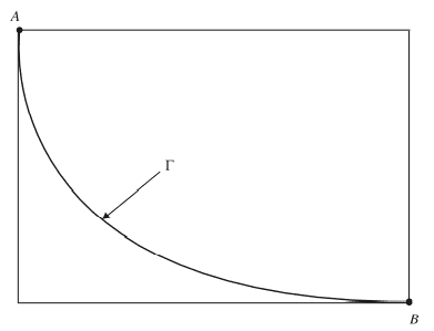
A celebrated problem first solved using the calculus of variations was the path of least time or the Brachistochrone problem. The problem is illustrated in Fig. 1.1. It involves finding the shape of a curve $\Gamma$ connecting the two points A and B in the vertical plane with the property that a bead sliding along the curve under the influence of gravity will move from A to B in the shortest possible time. The problem was posed by Johann Bernoulli in 1696, and it played an important part in the development of calculus of variations. It was solved by Johann Bernoulli, Jakob Bernoulli, Newton, Leibnitz, and L’Hôpital. In Sect. B.4, we provide a solution to the Brachistochrone problem by using what is known as the Euler-Lagrange equation, stated in Sect. B.2, and show that the shape of the solution curve is represented by a cycloid.
统计代写|最优控制作业代写optimal control代考|Notation and Concepts Used
In order to make the book readable, we will adopt the following notation which will hold throughout the book. In addition, we will define some important concepts that are required, including those of concave, convex and affine functions, and saddle points.
We use the symbol “=” to mean “is equal to” or “is defined to be equal to” or “is identically equal to” depending on the context. The symbol “:=” means “is defined to be equal to,” the symbol ” $\equiv$ ” means “is identically equal to,” and the symbol ” $\approx$ ” means “is approximately equal to.” The double arrow ” $\Rightarrow$ ” means “implies,” ” $\nabla$ ” means “for all,” and ” $\in$ ” means “is a member of.” The symbol $\square$ indicates the end of a proof.
Let $y$ be an $n$-component column vector and $z$ be an $m$-component row vector, i.e., $$ y=\left[\begin{array}{c} y_{1} \ y_{2} \ \vdots \ y_{n} \end{array}\right]=\left(y_{1}, \ldots, y_{n}\right)^{T} \text { and } z=\left(z_{1}, \ldots, z_{m}\right) $$ where the superscript ${ }^{T}$ on a vector (or, a matrix) denotes the transpose of the vector (or, the matrix). At times, when convenient and not confusing, we will use the superscript ${ }^{\prime}$ for the transpose operation. If $y$ and $z$ are functions of time $t$, a scalar, then the time derivatives $\dot{y}:=d y / d t$ and $\dot{z},=d z / d t$ are defined as $$ \dot{y}=\frac{d y}{d t}=\left(\dot{y}{1}, \cdots, \dot{y}{n}\right)^{T} \text { and } \dot{z}=\frac{d z}{d t}=\left(\dot{z}{1}, \ldots, \dot{z}{m}\right) $$ where $\dot{y}{i}$ and $\dot{z}{j}$ denote the time derivatives $d y_{i} / d t$ and $d z_{j} / d t$, respectively. Whēn $n=m$, we cann défine the iñner product $$ z y=\Sigma_{i=1}^{n} z_{i} y_{i} . $$
统计代写|最优控制作业代写optimal control代考|Basic Concepts and Definitions
We will use the word system as a primitive term in this book. The only property that we require of a system is that it is capable of existing in various states. Let the (real) variable $x(t)$ be the state variable of the system at time $t \in[0, T]$, where $T>0$ is a specified time horizon for the system under consideration. For example, $x(t)$ could measure the inventory level at time $t$, the amount of advertising goodwill at time $t$, or the amount of unconsumed wealth or natural resources at time $t$.
We assume that there is a way of controlling the state of the system. Let the (real) variable $u(t)$ be the control variable of the system at time $t$. For example, $u(t)$ could be the production rate at time $t$, the advertising rate at time $t$, etc.
Given the values of the state variable $x(t)$ and the control variable $u(t)$ at time $t$, the state equation, a differential equation, $$ \dot{x}(t)=f(x(t), u(t), t), \quad x(0)=x_{0}, $$ specifies the instantaneous rate of change in the state variable, where $\dot{x}(t)$ is a commonly used notation for $d x(t) / d t, f$ is a given function of $x, u$, and $t$, and $x_{0}$ is the initial value of the state variable. If we know the initial value $x_{0}$ and the control trajectory, i.e., the values of $u(t)$ over the whole time interval $0 \leq t \leq T$, then we can integrate (1.1) to get the state trajectory, i.e., the values of $x(t)$ over the same time interval. We want to choose the control trajectory so that the state and control trajectories maximize the objective functional, or simply the objective function, $$ J=\int_{0}^{T} F(x(t), u(t), t) d t+S[x(T), T] $$ In (1.2), $F$ is a given function of $x, u$, and $t$, which could measure the benefit minus the cost of advertising, the utility of consumption, the negative of the cost of inventory and production, etc. Also in (1.2), the function $S$ gives the salvage value of the ending state $x(T)$ at time $T$. The salvage value is needed so that the solution will make “good sense” at the end of the horizon.
统计代写|最优控制作业代写optimal control代考|Formulation of Simple Control Models
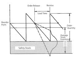
We now formulate three simple models chosen from the areas of production, advertising, and economics. Our only objective here is to identify and interpret in these models each of the variables and functions described in the previous section. The solutions for each of these models will be given in detail in later chapters. Example 1.1 A Production-Inventory Model. The various quantities that define this model are summarized in Table $1.1$ for easy comparison with the other models that rulluw.
We consider the production and inventory storage of a given good, such as steel, in order to meet an exogenous demand. The state variable $I(t)$ measures the number of tons of steel that we have on hand at time $t \in[0, T]$. There is an exogenous demand rate $S(t)$ tons of steel per day at time $t \in[0, T]$, and we must choose the production rate $P(t)$ tons of steel per day at time $t \in[0, T]$. Given the initial inventory of $I_{0}$ tons of steel on hand at $t=0$, the state equation $$ \dot{I}(t)=P(t)-S(t) $$ describes how the steel inventory changes over time. Since $h(I)$ is the cost of holding inventory $I$ in dollars per day, and $c(P)$ is the cost of producing steel at rate $P$, also in dollars per day, the objective function is to maximize the negative of the sum of the total holding and production costs over the period of $T$ days. Of course, maximizing the negative sum is the same as minimizing the sum of holding and production costs. The state variable constraint, $I(t) \geq 0$, is imposed so that the demand is satisfied for all $t$. In other words, backlogging of demand is not permitted. (An alternative formulation is to make $h(I)$ become very large when $I$ becomes negative, i.e., to impose a stockout penalty cost.) The control constraints keep the production rate $P(t)$ between a specified lower bound $P_{\min }$ and a specified upper bound $P_{\max }$. Finally, the terminal constraint $I(T) \geq I_{\min }$ is imposed so that the terminal inventory is at least $I_{\min }$.
The statement of the problem is lengthy because of the number of variables, functions, and parameters which are involved. However, with the production and inventory interpretations as given, it is not difficult to see the reasons for each condition. In Chap. 6, various versions of this model will be solved in detail. In Sect. $12.2$, we will deal with a stochastic version of this model.
统计代写|最优控制作业代写optimal control代考|Calculus of Variations
统计代写|最优控制作业代写optimal control代考|Calculus of Variations
We begin now the analysis of some optimization problems where the results about semiconcave functions and their singularities can be applied. In this chapter we consider what Fleming and Rishel [80] call “the simplest problem in the calculus of variations,” a case where the dynamic programming approach is particularly powerful, and which will serve as a guideline for the analysis of optimal control problems in the following.
The problem in the calculus of variations we study here has been introduced in Chapter 1, where some results have been given in the case where the integrand is independent of $t, x$. Here, we consider a general integrand, so that the minimizers no longer admit an explicit description as in the Hopf formula. However, the structure of minimizers is described by classical results: we give a result about existence and regularity of minimizers, and we show that they satisfy the well-known Euler-Lagrange equations. We then apply the dynamic programming approach and introduce the value function of the problem, which is semiconcave and is a viscosity solution of an associated Hamilton-Jacobi equation. The main purpose of our analysis is to study the singularities of the value function and their interpretation in the calculus of variations. For instance, we derive a correspondence between generalized gradients of the value function and the minimizing trajectories of the problem. This shows, in particular, that the singularities of the value function are exactly the endpoints for which the minimizer of the variational problem is not unique. In addition, we can bound the size of $\bar{\Sigma}$, the closure of the singular set, proving that it enjoys the same rectifiability properties of $\Sigma$ itself. This result is interesting because on the complement of $\bar{\Sigma}$ the value function has the same regularity as the data and can be computed by the method of characteristics.
The chapter is organized as follows. In Section $6.1$ we give the statement of the problem and the existence result for minimizers. In Section $6.2$ we show that minimizers are regular and derive the Euler-Lagrange equations. Starting from Section $6.3$ we focus our attention on problems with one free endpoint; we introduce the notions of irregular and conjugate point and we prove Jacobi’s necessary optimality condition. Then, in Section 6.4, we apply the dynamic programming approach to this problem. We show that the value function $u$ solves the associated Hamilton-Jacobi
equation in the viscosity sense and that it is semiconcave. In addition, the minimizers for the variational problem with a given final endpoint $(t, x)$ are in one-to-one correspondence with the elements of $D^{*} u(t, x)$; in particular, the differentiability of $u$ is equivalent to the uniqueness of the minimizer. We also show that $u$ is as regular as the data of the problem in the complement of the closure of its singular set $\Sigma$. The rest of the chapter is devoted to study the structure of $\bar{\Sigma}$. Since the properties of $\Sigma$ are well known from the general analysis of Chapter 4 , we focus our attention on the set $\bar{\Sigma} \backslash \Sigma$. The starting point is given in Section $6.5$, where we show that $\bar{\Sigma}=\Sigma \cup \Gamma$, where $\Gamma$ is the set of conjugate points. In addition, we prove some results about conjugate points showing, roughly speaking, that these are the points at which the singularities of $u$ are generated. Then, in Section $6.6$, we prove that $\Sigma$ has the same rectifiability property as $\Sigma$, i.e., it is a countably $\mathcal{H}^{\prime n}$-rectifiable subset of $\mathbb{R} \times \mathbb{R}^{n}$. By the previous remarks, this is equivalent to proving the rectifiability of $\Gamma \backslash \Sigma$. Combining a careful analysis of the hamiltonian system satisfied by the minimizing arcs with some tools from geometric measure theory, we obtain the finer estimate $$ \mathcal{H}^{n-1+\frac{2}{R-1}}(\Gamma \backslash \Sigma)=0, $$ where $k \geq 3$ is the differentiability class of the data. This yields in particular the desired Hausdorff estimate on $\bar{\Sigma}$, which shows that $u$ is as smooth as the data in the complement of a closed rectifiable set of codimension one.
统计代写|最优控制作业代写optimal control代考|Existence of minimizers
Let us consider the problem in the calculus of variations of Chapter 1 in a more general setting. We fix $T>0$, a connected open set $\Omega \subset \mathbb{R}^{n}$ and two closed subsets $S_{0}, S_{T} \subset \bar{\Omega}$. We denote by $\mathrm{AC}\left([0, T], \mathbb{R}^{n}\right)$ the class of all absolutely continuous arcs $\xi:[0, T] \rightarrow \mathbb{R}^{n}$ and define the set of admissible arcs by $$ \mathcal{A}=\left{\xi \in \mathrm{AC}\left([0, T], \mathbb{R}^{n}\right): \xi(t) \in \bar{\Omega} \text { for all } t \in[0, T], \xi(0) \in S_{0}, \xi(T) \in S_{T}\right} $$ Moreover, we define the functionals $\Lambda, J$ on $\mathcal{A}$ by $$ \Lambda(\xi)=\int_{0}^{T} L(s, \xi(s), \dot{\xi}(s)) d s $$ and $$ J(\xi)=\Lambda(\xi)+u_{0}(\xi(0))+u_{T}(\xi(T)) $$ Here $L:[0, T] \times \bar{\Omega} \times \mathbb{R}^{n} \rightarrow \mathbb{R}$ and $u_{0}, u_{T}: \bar{\Omega} \rightarrow \mathbb{R}$ are given continuous functions called running cost, initial cost and final cost, respectively, and $\Lambda$ is the action functional. We then consider the following minimization problem: (CV) Find $\xi_{} \in \mathcal{A}$ such that $J\left(\xi_{}\right)=\min {J(\xi): \xi \in \mathcal{A}}$.
统计代写|最优控制作业代写optimal control代考|Necessary conditions and regularity
We show in this section that the minimizing arcs for problem (CV) are regular and solve a system of equations called the Euler-Lagrange equations. Our analysis is restricted to those minimizers which are contained in $\Omega$; minimizers touching the boundary of $\Omega$ would require a longer analysis. We need some further assumptions on the data. Namely, we assume that the lagrangian $L$ is of class $C^{1}$ and that for all $r>0$ there exists $\mathcal{C}(r)>0$ such that $$ \begin{aligned} &\left|L_{x}(t, x, v)\right|+\left|L_{v}(t, x, v)\right| \leq \tilde{C}(r) \theta(|v|) \ &\forall t \in[0, T], x \in \bar{\Omega} \cap B_{r}, v \in \mathbb{R}^{n} \end{aligned} $$ where $\theta$ is the Nagumo function appearing in hypothesis (ii) of Theorem 6.1.2. Observe that property (iii) of the same theorem is implied by (6.6). In addition, we assume that $\theta$ satisfies $$ \theta(q+m) \leq K_{M}[1+\theta(q)] \quad \forall m \in[0, M], q \geq 0 $$ It is easily checked that assumption (6.7) is satisfied for many classes of superlinear functions $\theta$, such as powers or exponentials. It is violated in cases where $\theta$ grows “very fast”, e.g., $\theta(q)=e^{e q}, q \in \mathbb{R}$.
统计代写|最优控制作业代写optimal control代考|Calculus of Variations
Let $\Omega \subset \mathbb{R}^{n}$ be an open set and let $H \in C\left(\Omega \times \mathbb{R} \times \mathbb{R}^{n}\right)$. Let us again consider the general nonlinear first order equation $$ H(x, u, D u)=0, \quad x \in \Omega \subset \mathbb{R}^{n}, $$ in the unknown $u: \Omega \rightarrow \mathbb{R}$. As usual, evolution equations can be recast in this form by considering time as an additional space variable.
As we have already mentioned, when one considers boundary value problems or Cauchy problems for equations of the above form, one finds that in general no global smooth solutions exist even if the data are smooth. On the other hand, the property of being a Lipschitz continuous function satisfying the equation almost everywhere is usually too weak to have uniqueness results. Therefore, a crucial step in the analysis is to give a notion of a generalized solution such that global existence and uniqueness results can be obtained. In Chapter 1 we have seen a class of problems which are well posed in the class of semiconcave solutions. Here we present the notion of a viscosity solution, which has a much wider range of applicability.
Definition 5.2.1 A function $u \in C(\Omega)$ is called a viscosity subsolution of equation (5.14) if, for any $x \in \Omega$, it satisfies $$ H(x, u(x), p) \leq 0, \quad \forall p \in D^{+} u(x) . $$ Similarly, we say that $u$ is a viscosity supersolution of equation (5.14) if, for any $x \in \Omega$, we have $$ H(x, u(x), p) \geq 0, \quad \forall p \in D^{-} u(x) $$ If u satisfies both of the above properties, it is called a viscosity solution of equation (5.14).
Observe that, by virtue of Proposition 3.1.7, condition (5.15) (resp. (5.16)) can be restated in an equivalent way by requiring $$ H(x, u(x), D \phi(x)) \leq 0 \quad \text { (resp. } H(x, u(x), D \phi(x)) \geq 0 \text { ) } $$ for any $\phi \in C^{1}(\Omega)$ such that $u-\phi$ has a local maximum (resp. minimum) at $x$. We see that if $u$ is differentiable everywhere the notion of a viscosity solution coincides with the classical one since we have at any point $D^{+} u(x)=D^{-} u(x)=$ ${D u(x)}$. On the other hand, if $u$ is not differentiable everywhere, the definition of a viscosity solution includes additional requirements at the points of nondifferentiability. The reason for taking inequalities (5.15)-(5.16) as the definition of solution might not be clear at first sight, as well as the relation with the semiconcavity property considered in Chapter 1 . However, we will see that with this definition one can obtain existence and uniqueness results for many classes of Hamilton-Jacobi equations, and that the viscosity solution usually coincides with the one which is relevant for the applications, like the value function in optimal control. The relationship with semiconcavity will be examined in detail in the next section.
统计代写|最优控制作业代写optimal control代考|Semiconcavity and viscosity
We now analyze the relation between the notions of a semiconcave solution and a viscosity solution to Hamilton-Jacobi equations. We will see that the two notions are strictly related when the hamiltonian is a convex function of $D u$. We begin with the following result.
Proposition $5.3 .1$ Let u be a semiconcave function satisfying equation (5.14) almost everywhere. If $H$ is convex in the third argument, then $u$ is a viscosity solution of the equation.
Proof – As a first step. we show that $u$ satisfies the equation at all points of differentiability (our assumption is a priori slightly weaker). Let $u$ be differentiable at some $x_{0} \in \Omega$. Then there exists a sequence of points $x_{k}$ converging to $x_{0}$ such that (i) $u$ is differentiable at $x_{k}$; (ii) $H\left(x_{k}, u\left(x_{k}\right), D u\left(x_{k}\right)\right)=0$; (iii) $D u\left(x_{k}\right)$ has a limit for $k \rightarrow \infty$. From Proposition 3.3.4(a) we deduce that the limit of $D u\left(x_{k}\right)$ is $D u\left(x_{0}\right)$. By the continuity of $H$, the equation holds at $x_{0}$ as well.
Let us now take an arbitrary $x \in \Omega$ and check that (5.15) is satisfied. We first observe that $$ H(x, u(x), p)=0, \quad \forall p \in D^{} u(x) $$ This follows directly from the definition of $D^{} u$, the continuity of $H$ and the property that the equation holds at the points of differentiability. Since $D^{+} u(x)$ is the convex hull of $D^{*} u(x)$ (see Theorem $3.3 .6$ ) and $H$ is convex, inequality (5.15) follows. Now let us check inequality (5.16). For a given $x \in \Omega$, suppose that $D^{-} u(x)$ contains some vector $p$. Then, by Proposition 3.1.5(c) and Proposition 3.3.4(c), $u$ is differentiable at $x$ and $D u(x)=p$. Thus, $(5.16)$ holds as an equality by the first part of the proof.
Remark 5.3.2 A more careful analysis shows that the convexity of $H$ and the semiconcavity of $u$ play independent roles in the viscosity property. In fact, in the previous proof, the deduction that $u$ is a supersolution uses only semiconcavity and is valid also if $H$ is not convex. On the other hand, it is possible to prove (see see [110, p. 96] or [20, Prop. II.5.1]) that, if $H$ is convex, any Lipschitz continuous $u$ (not necessarily semiconcave) satisfying the equation almost everywhere is a viscosity subsolution of the equation.
统计代写|最优控制作业代写optimal control代考|Propagation of singularities
We now turn to the analysis of the singular set of semiconcave solutions to HamiltonJacobi equations. In Chapter 4 we have obtained results which are valid for any semiconcave function; here we focus our attention on semiconcave functions which are solutions to Hamilton-Jacobi equations and we obtain stronger results on the propagation of singularities in this case. As in the previous chapter, our discussion is restricted to semiconcave functions with linear modulus (some results in the case of a general modulus can be found in [1]). We consider again an equation of the form $$ F(x, u(x), D u(x))=0 \quad \text { a.e. in } \quad \Omega $$ Throughout the rest of this chapter, $F: \bar{\Omega} \times \mathbb{R} \times \mathbb{R}^{n} \rightarrow \mathbb{R}$ is a continuous function satisfying the following assumptions: (Al) $p \mapsto F(x, u, p)$ is convex; (A2) for any $(x, u) \in \Omega \times \mathbb{R}$ and any $p_{0}, p_{1} \in \mathbb{R}^{n}$, $$ \left\lfloor p_{0}, p_{1}\right] \subset\left{p \in \mathbb{R}^{n}: F(x, u, p)=0\right} \quad \Longrightarrow \quad p_{0}=p_{1} . $$ Condition (A2) requires that the 0 -level set $\left{p \in \mathbb{R}^{n}: F(x, u, p)=0\right}$ contains no straight line. Clearly, such a property holds, in particular, if $F$ is strictly convex with respect to $p$. Observe, however, that it also holds for functions like $F(x, u, p)=|p|$ which are not strictly convex.
Remark 5.4.1 In Proposition 5.3.1 we have seen that, under the convexity assumption (A1), any semiconcave function $u$ which solves equation (5.44) almost everywhere is also a viscosity solution of the equation. Thus, $u$ satisfies for all $x \in \Omega$ $$ \begin{array}{ll} F(x, u(x), p)=0 & \forall p \in D^{*} u(x) \ F(x, u(x), p) \leq 0 & \forall p \in D^{+} u(x) \end{array} $$ The first result we prove is that condition (4.8) is necessary and sufficient for the propagation of a singularity at $x_{0}$, if $u$ is a semiconcave solution of (5.44). Notice that, for a general semiconcave function, (4.8) is only a sufficient condition.
Theorem 5.4.2 Let (A1) and (A2) be satisfied. Let $u \in \mathrm{SCL}{l o c}(\Omega)$ be a solution of (5.44) and let $x{0} \in \Sigma(u)$. Then, the following properties are equivalent: (i) $\partial D^{+} u\left(x_{0}\right) \backslash D^{*} u\left(x_{0}\right) \neq \emptyset$; (ii) there exist a sequence $x_{i} \in \Sigma(u) \backslash\left{x_{0}\right}$, converging to $x_{0}$, and a number $\delta>0$ such that diam $D^{+} u\left(x_{i}\right) \geq \delta$, for any $i \in \mathbb{N}$.
统计代写|最优控制作业代写optimal control代考|Application to the distance function
统计代写|最优控制作业代写optimal control代考|Application to the distance function
In this section we examine some properties of the singular set of the distance function $d_{S}$ associated to a nonempty closed subset $S$ of $\mathbb{R}^{n}$. As in Section $3.4$, we denote by $\operatorname{proj}{S}(x)$ the set of closest points in $S$ to $x$, i.e., $$ \operatorname{proj}{S}(x)=\left{y \in S: d_{S}(x)=|x-y|\right} \quad x \in \mathbb{R}^{n} . $$ Our first result characterizes the isolated singularities of $d_{S}$. Theorem 4.4.1 Let $S$ be a nonempty closed subset of $\mathbb{R}^{n}$ and $x \notin S$ a singular point of $d_{5}$. Then the following properties are equivalent: (a) $x$ is an isolated point of $\Sigma\left(d_{S}\right)$. (b) $\partial D^{+} d_{S}(x)=D^{} d_{S}(x)$. (c) $\operatorname{proj}{S}(x)=\partial B{r}(x)$ where $r:=d_{S}(x)$. Proof – The implication (a) $\Rightarrow$ (b) is an immediate corollary of the propagation result of Section 4.2. Indeed, if $\partial D^{+} d_{S}(x) \backslash D^{} d S(x)$ is nonempty, then Theorem 4.2.2 ensures the existence of a nonconstant singular arc with initial point $x$. In particular, $x$ could not be isolated.
Let us now show that (b) implies (c). First, we claim that, if (b) holds, then $x$ must be a singular point of magnitude $\kappa(x)=n$, i.e., $\operatorname{dim} D^{+} d s(x)=n$. For suppose the strict inequality $\kappa(x)} d_{S}(x)$. Therefore, $D^{+} d_{S}(x) \subset \partial B_{1}$ as all reachable gradients of $d_{S}$ are unit vectors. But the last inclusion contradicts the fact that $D^{+} d S(x)$ is a convex set of dimension at least 1. Our claim is thus proved. Now, we use the fact that $D^{+} d_{S}(x)$ is an $n$-dimensional convex set with $$ \partial D^{+} d_{S}(x)=D^{} d_{S}(x) \subset \partial B_{1} $$ to conclude that $D^{+} d_{S}(x)=\bar{B}{1}$ and $D^{} d{S}(x)=\partial B_{1}$. Then, we invoke formula (3.40) to discover $$ \operatorname{proj}{S}(x)=x-d{S}(x) D^{} d_{S}(x)=\partial B_{r}(x), $$ which proves (c). Finally, let us show that (c) implies (a). From Corollary 3.4.5 (iii) we know that $d s$ is differentiable along each segment $] x, y\left[\right.$ with $y \in \operatorname{proj}{S}(x)=\partial B{r}(x)$. So, $d_{S} \in C^{1}\left(B_{r}(x) \backslash{x}\right)$ and the proof is complete.
In other words, the previous result shows that a point $x_{0}$ is an isolated singularity for the distance function from a set $S$ only if there exists an open sphere $B$ centered at $x_{0}$, such that $B \cap S=\emptyset$ and $\partial B \subset S$. In particular, if $S$ is a simply connected set in $\mathbb{R}^{2}$, or a set in $\mathbb{R}^{n}$ with trivial $n-1$ homotopy group, then the distance from $S$ has no isolated singularities in the complement of $S$.
Hamilton-Jacobi equations are nonlinear first order equations which have been first introduced in classical mechanics, but find application in many other fields of mathematics. Our interest in these equations lies mainly in the connection with calculus of variations and optimal control. We have seen in Chapter 1 how the dynamic programming approach leads to the analysis of a Hamilton-Jacobi equation and other examples will be considered in the remainder of the book. However, our point of view in this chapter will be to study Hamilton-Jacobi equations for their intrinsic interest without referring to specific applications.
We begin by giving, in Section 5.1, a fairly general exposition of the method of characteristics. This method allows us to construct smooth solutions of first order equations, and in general can be applied only locally. However, this method is interesting also for the study of solutions that are not smooth. As we will see in the following, characteristic curves (or suitable generalizations) often play an important role for generalized solutions and are related to the optimal trajectories of the associated control problem.
In Section $5.2$ we recall the basic definitions and results from the theory of viscosity solutions for Hamilton-Jacobi equations. In this theory solutions are defined by means of inequalities satisfied by the generalized differentials or by test functions. With such a definition it is possible to obtain existence and uniqueness theorems under quite general hypotheses. In addition, in most cases where the equation is associated to a control problem, the viscosity solution coincides with the value function of the problem. Although this section is meant to be a collection of results whose proof can be found in specialized monographs, we have included the proofs of some simple statements in order to give to the reader the flavor of the techniques of the theory.
In Section $5.3$ we analyze the relation between semiconcavity and the viscosity property. Roughly speaking, it turns out that the two properties are equivalent when the hamiltonian is a convex function of the gradient of the solution. However, it is also possible to obtain semiconcavity results under different assumptions on the hamiltonian.
统计代写|最优控制作业代写optimal control代考|Method of characteristics
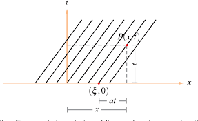
In Section $1.5$ we have introduced the method of characteristics to construct a local classical solution of the Cauchy problem for equations of the form $\partial_{t} u+H(\nabla u)=0$. We now show how this method can be extended to study general first order equations. As a first step, let us show how the procedure of Section $1.5$ can be generalized to Cauchy problems where the hamiltonian depends also on $t, x$. Let us consider the problem $$ \begin{gathered} \partial_{t} u(t, x)+H(t, x, \nabla u(t, x))=0, \quad(t, x) \in\left[0, \infty\left[\times \mathbb{R}^{n}\right.\right. \ u(0, x)=u_{0}(x), \quad x \in \mathbb{R}^{n}, \end{gathered} $$ with $H$ and $u_{0}$ of class $C^{2}$. Suppose, first, we have a solution $u \in C^{2}\left([0, T] \times \mathbb{R}^{n}\right)$ of the above problem. Given $z \in \mathbb{R}^{n}$, we call characteristic curve associated to $u$ starting from $z$ the curve $t \rightarrow(t, X(t ; z))$, where $X(* ; z)$ solves $$ \dot{X}=H_{p}(t, X, \nabla u(t, X)), \quad X(0)=z . $$ Here and in the following the dot denotes differentiation with respect to $t$. Now, if we set $$ U(t ; z)=u(t, X(t ; z)), \quad P(t ; z)=\nabla u(t, X(t ; z)) $$ we find that $$ \begin{gathered} \dot{U}=u_{t}(t, X)+\nabla u(t, X) \cdot \dot{X}=-H(t, X, P)+P \cdot H_{p}(t, X, P) \ \dot{P}=\nabla u_{t}(t, X)+\nabla^{2} u(t, X) H_{p}(t, X, \nabla u(t, X)) \end{gathered} $$ Taking into account that $$ \begin{aligned} 0 &=\nabla\left(u_{t}(t, x)+H(t, x, \nabla u(t, x))\right) \ &=\nabla u_{t}(t, x)+H_{x}(t, x, \nabla u(t, x))+\nabla^{2} u(t, x) H_{p}(t, x, \nabla u(t, x)) \end{aligned} $$ we obtain that $$ \dot{P}=-H_{x}(t, X, \nabla u(t, X))=-H_{x}(t, X, P) $$
统计代写|最优控制作业代写optimal control代考|Application to the distance function
统计代写|最优控制作业代写optimal control代考|Singularities of Semiconcave Functions
统计代写|最优控制作业代写optimal control代考|Singularities of Semiconcave Functions
By a singular point, or singularity, of a semiconcave function $u$ we mean a point where $u$ is not differentiable. This chapter is devoted to the analysis of the set of all singular points for $u$, which is called singular set and is denoted here by $\Sigma(u)$. As we have already remarked, the singular set of a semiconcave function has zero measure by Rademacher’s theorem. However, we will see that much more detailed properties can be proved.
In Section $4.1$ we study the rectifiability properties of the singular set. We divide the singular points according to the dimension of the superdifferential of $u$ denoting by $\Sigma^{k}(u)$ the set of points $x$ such that $D^{+} u(x)$ has dimension $k$. Then we show that $\Sigma^{k}(u)$ is countably $(n-k)$-rectifiable for all integers $k=1, \ldots, n$. In particular, the whole singular set $\Sigma(u)$ is countably ( $n-1)$-rectifiable.
Sections $4.2$ and $4.3$ are devoted to the propagation of singularities for semiconcave functions: given a singular point $x_{0}$, we look for conditions ensuring that $x_{0}$ belongs to a connected component of dimension $v \geq 1$ of the singular set. We study first the propagation along Lipschitz arcs and then along Lipschitz manifolds of higher dimension. In general we find that a sufficient condition for the propagation of singularities from $x_{0}$ is that the inclusion $D^{*} u\left(x_{0}\right) \subset \partial D^{+} u\left(x_{0}\right)$ (see Proposition 3.3.4-(b) ) is strict.
As an application of the previous analysis, we study in Section $4.4$ some properties of the distance function from a closed set $S$. Using our propagation results, we show that the distance function has no isolated singularities except for the special case when the singularity is the center of a spherical connected component of the complement of $S$. In general, we show that a point $x_{0}$ which is singular for the distance function belongs to a connected set of singular points whose Hausdorff dimension is at least $n-k$, with $k=\operatorname{dim}\left(D^{+} d\left(x_{0}\right)\right)$.
统计代写|最优控制作业代写optimal control代考|Rectifiability of the singular sets
Throughout this chapter $\Omega \subset \mathbb{R}^{n}$ is an open set and $u: \Omega \rightarrow \mathbb{R}$ is a semiconcave function. We denote by $\Sigma(u)$ the set of points of $\Omega$ where $u$ is not differentiable and
we call it the singular set of $u$. In the following we use some notions from measure theory, like Hausdorff measures and rectifiable sets, which are recalled in Appendix A. 3 .
We know from Theorem 2.3.1-(ii) that $D u$ is a function with bounded variation if $u$ is semiconcave with a linear modulus. For functions of bounded variation one can introduce the jump set, whose rectifiability properties have been widely studied (see Appendix A. 6). We now show that the jump set of $D u$ coincides with the singular set $\Sigma(u)$. To this purpose we need two preliminary results. The first one is a lemma about approximate limits (see Definition A. 6.2).
Lemma 4.1.1 Let $w \in L^{1}(A)$, with $A \subset \mathbb{R}^{n}$ open, let $\bar{x} \in A$, and let ap $\lim {x \rightarrow \bar{x}} w(x)=\bar{w}$. Then for any $\theta \in \mathbb{R}^{n}$ with $|\theta|=1$ we can find a sequence $\left{x{k}\right} \subset A$ such that $$ x_{k} \rightarrow \bar{x}, \quad \frac{x_{k}-\bar{x}}{\left|x_{k}-\bar{x}\right|} \rightarrow \theta, \quad w\left(x_{k}\right) \rightarrow \bar{w} \quad \text { as } k \rightarrow \infty $$ Proof – For any $k \in \mathbb{N}$, let us define $$ A_{k}=\left{x \in A \backslash{\bar{x}}:\left|\frac{x-\bar{x}}{|x-\bar{x}|}-\theta\right|<\frac{1}{k}\right} $$ Any such set $A_{k}$ is the intersection of $A$ with an open cone of vertex $\bar{x}$. Therefore $$ \lim {\rho \rightarrow 0^{+}} \frac{\text { meas }\left(B{\rho}(\bar{x}) \cap A_{k}\right)}{\rho^{n}}>0 . $$ By the definition of approximate limit we have $$ \lim {\rho \rightarrow 0^{+}} \frac{\operatorname{meas}\left(\left{x \in B{\rho}(\bar{x}) \cap A_{k}:|w(x)-\bar{w}|>1 / k\right}\right)}{\rho^{n}}=0 . $$ Comparing the above relations we see that the set $$ \left{x \in B_{\rho}(\bar{x}) \cap A_{k}:|w(x)-\bar{w}| \leq 1 / k\right} $$ is nonempty if $\rho$ is small enough. Thus, we can find $x_{k} \in A_{k}$ such that $\left|w\left(x_{k}\right)-\bar{w}\right| \leq$ $1 / k,\left|x_{k}-\bar{x}\right| \leq 1 / k$. Repeating this construction for all $k$ we obtain a sequence $\left{x_{k}\right}$ with the desired properties.
Next we give a result showing, roughly speaking, that for the gradient of a semiconcave function the notions of limit and of approximate limit coincide.
统计代写|最优控制作业代写optimal control代考|Propagation along Lipschitz arcs
Let $u$ be a semiconcave function in an open domain $\Omega \subseteq \mathbb{R}^{n}$. The rectiflability properties of $\Sigma(u)$, obtained in the previous section, can be regarded as “upper bounds” for $\Sigma(u)$. From now on, we shall study the singular set of $u$ trying to obtain “lower bounds” for such a set. In the rest of the chapter, we restrict our attention to semiconcave functions with a linear modulus.
Given a point $x_{0} \in \Sigma(u)$, we are interested in conditions ensuring the existence of other singular points approaching $x_{0}$. The following example explains the nature of such conditions. Example 4.2.1 The functions $$ u_{1}\left(x_{1}, x_{2}\right)=-\sqrt{x_{1}^{2}+x_{2}^{2}}, \quad u_{2}\left(x_{1}, x_{2}\right)=-\left|x_{1}\right|-\left|x_{2}\right| $$ are concave in $\mathbb{R}^{2}$, and $(0,0)$ is a singular point for both of them. Moreover, $(0,0)$ is the only singularity for $u_{1}$ while $$ \Sigma\left(u_{2}\right)=\left{\left(x_{1}, x_{2}\right): x_{1} x_{2}=0\right} $$ So, $(0,0)$ is the intersection point of two singular lines of $u_{2}$. Notice that $(0,0)$ has magnitude 2 with respect to both functions as $$ \begin{gathered} D^{+} u_{1}(0,0)=\left{\left(p_{1}, p_{2}\right): p_{1}^{2}+p_{2}^{2} \leq 1\right} \ D^{+} u_{2}(0,0)=\left{\left(p_{1}, p_{2}\right):\left|p_{1}\right| \leq 1,\left|p_{2}\right| \leq 1\right} \end{gathered} $$ The different structure of $\Sigma\left(u_{1}\right)$ and $\Sigma\left(u_{2}\right)$ in a neighborhood of $x_{0}$ is captured by the reachable gradients. In fact, $$ \begin{gathered} D^{} u_{1}(0,0)=\left{\left(p_{1}, p_{2}\right): p_{1}^{2}+p_{2}^{2}=1\right}=\partial D^{+} u_{1}(0,0) \ D^{} u_{2}(0,0)=\left{\left(p_{1}, p_{2}\right):\left|p_{1}\right|=1,\left|p_{2}\right|=1\right} \neq \partial D^{+} u_{2}(0,0) \end{gathered} $$ In other words, the inclusion $D^{*} u(x) \subset \partial D^{+} u(x)$ (see Proposition 3.3.4(b)) is an equality for $u_{1}$ and a proper inclusion for $u_{2}$.
The above example suggests that a sufficient condition to exclude that $x_{0}$ is an isolated point of $\Sigma(u)$ should be that $D^{*} u\left(x_{0}\right)$ fails to cover the whole boundary of $D^{+} u\left(x_{0}\right)$. As we shall see, such a condition implies a much stronger property, namely that $x_{0}$ is the initial point of a Lipschitz singular arc.
In the following we call an arc a continuous map $\mathbf{x}:[0, \rho] \rightarrow \mathbb{R}^{n}, \rho>0$. We shall say that the arc $\mathbf{x}$ is singular for $u$ if the support of $\mathbf{x}$ is contained in $\Omega$ and $\mathbf{x}(s) \in \Sigma(u)$ for every $s \in[0, \rho]$. The following result describes the “arc structure” of the singular set $\Sigma(u)$.
统计代写|最优控制作业代写optimal control代考|Singularities of Semiconcave Functions
统计代写|最优控制作业代写optimal control代考|Superdifferential of a semiconcave function
统计代写|最优控制作业代写optimal control代考|Superdifferential of a semiconcave function
The superdifferential of a semiconcave function enjoys many properties that are not valid for a general Lipschitz continuous function, and that can be regarded as extensions of analogous properties of concave functions. We start with the following basic estimate. Throughout the section $A \subset \mathbb{R}^{n}$ is an open set.
Proposition 3.3.1 Let $u: A \rightarrow \mathbb{R}$ be a semiconcave function with modulus $\omega$ and let $x \in A$. Then, a vector $p \in \mathbb{R}^{n}$ belongs to $D^{+} u(x)$ if and only if $$ u(y)-u(x)-\langle p, y-x\rangle \leq|y-x| \omega(|y-x|) $$ Jor any pont y EA such that $[y, r\rfloor$ s. $_{-}$
Proof – If $p \in \mathbb{R}^{n}$ satisfies (3.18), then, by the very definition of superdifferential, $p \in D^{+} u(x)$. In order to prove the converse, let $p \in D^{+} u(x)$. Then, dividing the semiconcavity inequality $(2.1)$ by $(1-\lambda)|x-y|$, we have $$ \left.\left.\frac{u(y)-u(x)}{|y-x|} \leq \frac{u(x+(1-\lambda)(y-x))-u(x)}{(1-\lambda)|y-x|}+\lambda \omega(|x-y|), \quad \forall \lambda \in\right] 0,1\right] . $$ Hence, taking the limit as $\lambda \rightarrow 1^{-}$, we obtain $$ \frac{u(y)-u(x)}{|y-x|} \leq \frac{\langle p, y-x\rangle}{|y-x|}+\omega(|x-y|), $$ since $p \in D^{+} u(x)$. Estimate (3.18) follows. Remark 3.3.2 In particular, if $u$ is concave on a convex set $A$. we find that $p \in$ $D^{+} u(x)$ if and only if $$ u(y) \geq u(x)+\langle p, y-x\rangle, \quad \forall y \in A . $$ In convex analysis (see Appendix A. 1) this property is usually taken as the definition of the superdifferential. Therefore, the Fréchet super- and subdifferential coincide with the classical semidifferentials of convex analysis in the case of a concave (resp. convex) function.
Before investigating further properties of the superdifferential, let us show how Proposition 3.3.1 easily yields a compactness property for semiconcave functions.
统计代写|最优控制作业代写optimal control代考|Marginal functions
A function $u: A \rightarrow \mathbb{R}$ is called a marginal function if it can be written in the form $$ u(x)=\inf _{s \in S} F(s, x), $$ where $S$ is some topological space and the function $F: S \times A \rightarrow \mathbb{R}$ depends smoothly on $x$. Functions of this kind appear often in the literature, sometimes with different names (see e.g., the lower $C^{k}$-functions in [123]).
Under suitable regularity assumptions for $F$, a marginal function is semiconcave. For instance, Corollary $2.1 .6$ immediately implies the following. Proposition 3.4.1 Let $A \subset \mathbb{R}^{n}$ be open and let $S \subset \mathbb{R}^{m}$ be compact. If $F=F(s, x)$ is continuous in $C(S \times A)$ together with its partial derivatives $D_{x} F$, then the function u defined in (3.34) belongs to $\mathrm{SC}{l o c}(A)$. If $D{x x}^{2} F$ also exists and is continuous in $S \times A$, then $u \in \mathrm{SCL}{l o c}(A)$. We now show that the converse also holds. Theorem 3.4.2 Let $u: A \rightarrow \mathbb{R}$ be a semiconcave function. Then $u$ can be locally written as the minimum of functions of class $C^{1}$. More precisely, for any $K \subset A$ compact, there exists a compact set $S \subset \mathbb{R}^{2 n}$ and a continuous function $F: S \times K \rightarrow$ $\mathbb{R}$ such that $F(s, \cdot)$ is $C^{1}$ for any $s \in S$, the gradients $D{x} F(s, \cdot)$ are equicontinuous, and $$ u(x)=\min _{s \in S} F(s, x), \quad \forall x \in K . $$ If the modulus of semiconcavity of $u$ is linear, then $F$ can be chosen such that $F(s,-)$ is $C^{2}$ for any $s$, with uniformly bounded $C^{2}$ norm.
Proof – Let $\omega$ be the modulus of semiconcavity of $u$ and let $\omega_{1}$ be a function such that $\omega_{1}(0)=0$, that $\omega_{1}(r) \geq \omega(r)$ and that the function $x \rightarrow|x| \omega_{1}(|x|)$ belongs to $C^{1}\left(\mathbb{R}^{n}\right)$. The existence of such an $\omega_{1}$ has been proved in Lemma 3.1.8. If $\omega$ is linear we simply take $\omega_{1} \equiv \omega$.
Let us set $S=\left{(y, p): y \in K, p \in D^{+} u(y)\right}$. By Proposition 3.3.4(a) and the local Lipschitz continuity of $u, S$ is a compact set. Then we define $$ F(y, p, x)=u(y)+\langle p, x-y\rangle+|y-x| \omega_{1}(|y-x|) $$ Then $F$ has the required regularity properties. In addition $F(y, p, x) \geq u(x)$ for all $(y, p, x) \in S \times K$ by Proposition 3.3.1. On the other hand, if $x \in K$, then $D+u(x)$ is nonempty and so thêré exists at lesast a vectō $p$ such that $(x, p) \in S$. Since $F(x, p, x)=u(x)$, we obtain $(3.35)$.
If $u$ is semiconcave with a linear modulus, then it admits another representation as the infimum of regular functions by a procedure that is very similar to the Legendre transformation.
统计代写|最优控制作业代写optimal control代考|Inf-convolutions
Given $g: \mathbb{R}^{n} \rightarrow \mathbb{R}$ and $\varepsilon>0$, the functions $$ x \rightarrow \inf {y \in \mathbb{R}^{n}}\left(g(y)+\frac{|x-y|^{2}}{2 \varepsilon}\right) \quad x \rightarrow \sup {y \in \mathbb{R}^{n}}\left(g(y)-\frac{|x-y|^{2}}{2 \varepsilon}\right) $$ are called inf- and sup-convolutions of $g$ respectively, due to the formal analogy with the usual convolution. They have been used in various contexts as a way to approximate $g$; one example is the uniqueness theory for viscosity solutions of HamiltonJacobi equations. In some cases it is useful to consider more general expressions, where the quadratic term above is replaced by some other coercive function. In this section we analyze such general convolutions, showing that their regularity properties are strictly related with the properties of semiconcave functions studied in the previous sections. Definition 3.5.1 Let $g \in C\left(\mathbb{R}^{n}\right)$ satisfy $$ |g(x)| \leq K(1+|x|) $$ for some $K>0$ and let $\phi \in C\left(\mathbb{R}^{n}\right)$ be such that
$$ \lim {|q| \rightarrow+\infty} \frac{\phi(q)}{|q|}=+\infty . $$ The inf-convolution of $g$ with kernel $\phi$ is the function $$ g \phi(x)=\inf {y \in \mathbb{R}^{a}}[g(y)+\phi(x-y)], $$ while the sup-convolution of $g$ with kernel $\phi$ is defined by $$ g^{\phi}(x)=\sup {y \in \mathbb{R}^{n}}[g(y)-\phi(x-y)] . $$ We observe that the function $u$ given by Hopf’s formula (1.10) is an infconvolution with respect to the $x$ variable for any fixed $t$. In addition, inf-convolutions are a particular case of the marginal functions introduced in the previous section. We give below some regularity properties of the inf-convolutions. The corresponding statements about the sup-convolutions are easily obtained observing that $g^{\phi}=-\left((-g){\phi}\right)$.
统计代写|最优控制作业代写optimal control代考|Superdifferential of a semiconcave function
统计代写|最优控制作业代写optimal control代考|Generalized Gradients and Semiconcavity
统计代写|最优控制作业代写optimal control代考|Generalized Gradients and Semiconcavity
In the last decades a branch of mathematics has developed called nonsmooth analysis, whose object is to generalize the basic tools of calculus to functions that are not differentiable in the classical sense. For this purpose, one introduces suitable notions of generalized differentials, which are extensions of the usual gradient; the best known example is the subdifferential of convex analysis. The motivation for this study is that in more and more fields of analysis, like the optimization problems considered in this book, the functions that come into play are often nondifferentiable. For semiconcave functions, the analysis of generalized gradients is important in view of applications to control theory. As we have already seen in a special case (Corollary 1.5.10), if the value function of a control problem is smooth, then one can design the optimal trajectories knowing the differential of the value function. In the general case, where the value function is not smooth but only semiconcave, one can try to follow a similar procedure starting from its generalized gradient.
In Section $3.1$ we define the generalized differentials which are relevant for our purposes and recall basic properties and equivalent characterizations of these objects. Then, we restrict ourselves to semiconcave functions. In Section $3.2$ we show that semiconcave functions possess one-sided directional derivatives everywhere, while in Section $3.3$ we describe the special properties of the superdifferential of a semiconcave function; in particular, we show that it is nonempty at every point and that it is a singleton exactly at the points of differentiability. These properties are classical in the case of concave functions; here we prove that they hold for semiconcave functions with arbitrary modulus.
Section $3.4$ is devoted to the so-called marginal functions, which are obtained as the infimum of smooth functions. We show that semiconcave functions can be characterized as suitable classes of marginal functions. In addition, we describe the semi-differentials of a marginal function using the general results of the previous sections. In Section $3.5$ we study the so-called inf-convolutions. They are marginal functions defined by a process which is a generalization of Hopf’s formula, and provide approximations to a given function which enjoy useful properties. Finally, in Section $3.6$ we introduce proximal gradients and proximally smooth sets, and we analyze how these notions are related to semiconcavity.
We begin with the definitions of some generalized differentials and derivatives from nonsmooth analysis. In this section $u$ is a real-valued function defined on an open set $A \subset \mathbb{R}^{n}$. Definition 3.1.1 For any $x \in A$, the sets $$ \begin{aligned} D^{-} u(x) &=\left{p \in \mathbb{R}^{n}: \liminf {y \rightarrow x} \frac{u(y)-u(x)-\langle p, y-x\rangle}{|y-x|} \geq 0\right} \ D^{+} u(x) &=\left{p \in \mathbb{R}^{n}: \limsup {y \rightarrow x} \frac{u(y)-u(x)-\langle p, y-x\rangle}{|y-x|} \leq 0\right} \end{aligned} $$ are called, respectively, the (Fréchet) superdifferential and subdifferential of $u$ at $x$. From the definition it follows that, for any $x \in A$, $$ D^{-}(-u)(x)=-D^{+} u(x) . $$ Example 3.1.2 Let $A=\mathbb{R}$ and let $u(x)=|x|$. Then it is easily seen that $D^{+} u(0)=\emptyset$ whereas $D^{-} u(0)=[-1,1] .$ Let $A=\mathbb{R}$ and let $u(x)=\sqrt{|x|}$. Then, $D^{+} u(0)=\emptyset$ whereas $D^{-} u(0)=\mathbb{R}$. Let $A=\mathbb{R}^{2}$ and $u(x, y)=|x|-|y|$. Then, $D^{+} u(0,0)=D^{-} u(0,0)=\emptyset$. Definition 3.1.3 Let $x \in A$ and $\theta \in \mathbb{R}^{n}$. The upper and lower Dini derivatives of $u$ at $x$ in the direction $\theta$ are defined as $$ \partial^{+} u(x, \theta)=\lim {h \rightarrow 0^{+}, \theta^{\prime} \rightarrow \theta} \frac{u\left(x+h \theta^{\prime}\right)-u(x)}{h} $$ and $$ \partial^{-} u(x, \theta)=\liminf {h \rightarrow 0^{+}, \theta^{\prime} \rightarrow \theta} \frac{u\left(x+h \theta^{\prime}\right)-u(x)}{h}, $$ respectively. It is readily seen that, for any $x \in A$ and $\theta \in \mathbb{R}^{n}$ $$ \partial^{-}(-u)(x, \theta)=-\partial^{+} u(x, \theta) . $$ Remark 3.1.4 Whenever $u$ is Lipschitz continuous in a neighborhood of $x$, the lower Dini derivative reduces to $$ \partial^{-} u(x, \theta)=\liminf _{h \rightarrow 0+} \frac{u(x+h \theta)-u(x)}{h} $$ for any $\theta \in \mathbb{R}^{n}$. Indeed, if $L>0$ is the Lipschitz constant of $u$ we have $$ \left|\frac{u\left(x+h \theta^{\prime}\right)-u(x)}{h}-\frac{u(x+h \theta)-u(x)}{h}\right| \leq L\left|\theta^{\prime}-\theta\right|, $$ and (3.5) easily follows. A similar property holds for the upper Dini derivative.
We begin our exposition of the differential properties of semiconcave functions showing that they possess (one-sided) directional derivatives $$ \partial u(x, \theta):=\lim {h \rightarrow 0^{+}} \frac{u(x+h \theta)-u(x)}{h} $$ at any point $x$ and in any direction $\theta$. Theorem 3.2.1 Let $u: A \rightarrow \mathbb{R}$ be semiconcave. Then, for any $x \in A$ and $\theta \in \mathbb{R}^{n}$, $$ \partial u(x, \theta)=\partial^{-} u(x, \theta)=\partial^{+} u(x, \theta)=u{-}^{0}(x, \theta) . $$ Proof – Let $\delta>0$ be fixed so that $B_{\delta|\theta|}(x) \subset A$. Then, for any pair of numbers $h_{1}, h_{2}$ satisfying $0<h_{1} \leq h_{2}<\delta$, estimate (2.1) yields $$ \left(1-\frac{h_{1}}{h_{2}}\right) u(x)+\frac{h_{1}}{h_{2}} u\left(x+h_{2} \theta\right)-u\left(x+h_{1} \theta\right) \leq h_{1}\left(1-\frac{h_{1}}{h_{2}}\right)|\theta| \omega\left(h_{2}|\theta|\right) . $$ Hence, $$ \begin{aligned} &\frac{u\left(x+h_{1} \theta\right)-u(x)}{h_{1}} \ &\geq \frac{u\left(x+h_{2} \theta\right)-u(x)}{h_{2}}-\left(1-\frac{h_{1}}{h_{2}}\right)|\theta| \omega\left(h_{2}|\theta|\right) . \end{aligned} $$ Taking the liminf as $h_{1} \rightarrow 0^{+}$in both sides of the above inequality, we obtain
$$ \partial^{-} u(x, \theta) \geq \frac{u\left(x+h_{2} \theta\right)-u(x)}{h_{2}}-|\theta| \omega\left(h_{2}|\theta|\right) $$ Now, taking the limsup as $h_{2} \rightarrow 0^{+}$, we conclude that $$ \partial^{-} u(x, \theta) \geq \partial^{+} u(x, \theta) . $$ So, $\partial u(x, \theta)$ exists and coincides with the lower and upper Dini derivatives. To complete the proof of $(3.15)$ it suffices to show that $$ \partial^{+} u(x, \theta) \leq u_{-}^{0}(x, \theta), $$ since the reverse inequality holds by definition and by Remark 3.1.4. For this purpose, let $\varepsilon>0, \lambda \in] 0, \delta[$ be fixed. Since $u$ is continuous, we can find $\alpha \in$ ] $0,(\delta-\lambda) \theta$ [ such that $$ \frac{u(x+\lambda \theta)-u(x)}{\lambda} \leq \frac{u(y+\lambda \theta)-u(y)}{\lambda}+\varepsilon, \quad \forall y \in B_{\alpha}(x) . $$ Using inequality (3.16) with $x$ replaced by $y$, we obtain $$ \left.\frac{u(y+\lambda \theta)-u(y)}{\lambda} \leq \frac{u(y+h \theta)-u(y)}{h}+|\theta| \omega(\lambda|\theta|), \quad \forall h \in\right] 0, \lambda[. $$ Therefore, $$ \frac{u(x+\lambda \theta)-u(x)}{\lambda} \leq \inf {y \in B{u}(x), h \in|0, \lambda|} \frac{u(y+h \theta)-u(y)}{h}+|\theta| \omega(\lambda|\theta|)+\varepsilon . $$ This implies, by definition of $u_{-}^{0}(x, \theta)$, that $$ \frac{u(x+\lambda \theta)-u(x)}{\lambda} \leq u_{-}^{0}(x, \theta)+|\theta| \omega(\lambda|\theta|)+\varepsilon . $$ Hence, taking the limit as $\varepsilon, \lambda \rightarrow 0$, we obtain inequality (3.17).
统计代写|最优控制作业代写optimal control代考|Generalized Gradients and Semiconcavity
统计代写|最优控制作业代写optimal control代考|Special properties of SCL
统计代写|最优控制作业代写optimal control代考|Special properties of SCL
While many properties of semiconcave functions are valid in the case of an arbitrary modulus of semiconcavity, there are some results which are peculiar to the case of a linear modulus; we collect in this section some important ones, in addition to those already given in Proposition 1.1.3.
We have seen in Proposition 1.1.3 that semiconcave functions with a linear modulus can be regarded as $C^{2}$ perturbations of concave functions. This allows to extend immediately some well-known properties of concave functions, such as the following.
Theorem 2.3.1 Let $u \in \mathrm{SCL}(A)$, with $A \subset \mathbb{R}^{n}$ open. Then the following properties hold. (i) (Alexandroff’s Theorem) $u$ is twice differentiable a.e, that is, for a.e. every $x_{0} \in A$, there exist a vector $p \in \mathbb{R}^{n}$ and a symmetric matrix $B$ such that $$ \lim {x \rightarrow x{0}} \frac{u(x)-u\left(x_{0}\right)-\left\langle p, x-x_{0}\right)+\left\langle B\left(x-x_{0}\right), x-x_{0}\right\rangle}{\left|x-x_{0}\right|^{2}}=0 . $$ (ii) The gradient of u, defined almost everywhere in A, belongs to the class $\mathrm{BV}_{\text {loc }}\left(A, \mathbb{R}^{n}\right)$. Proof – Properties (i) and (ii) hold for a convex function (see e.g., $[72$, Ch. 6.3]). Since $u$ is the difference of a smooth function and a convex one, $u$ also satisfies these properties.
The following result shows that semiconcave functions with linear modulus exhibit a behavior similar to $C^{2}$ functions near a minimum point.
Theorem 2.3.2 Let $u \in \mathrm{SCL}(A)$, with $A \subset \mathbb{R}^{n}$ open, and let $x_{0} \in A$ be a point of local minimum for $u$. Then there exist a sequence $\left{x_{h}\right} \subset A$ and an infinitesimal sequence $\left{\varepsilon_{h}\right} \subset \mathbb{R}+$ such that $u$ is $t$ wice differentiable in $x_{h}$ and that $$ \lim {h \rightarrow \infty} x{h}=x_{0}, \quad \lim {h \rightarrow \infty} D u\left(x{h}\right)=0, \quad D^{2} u\left(x_{h}\right) \geq-\varepsilon_{h} I \quad \forall h . $$ The proof of this theorem is based on the following result.
Let us consider the parabolic Hamilton-Jacobi equation $$ \partial_{f} u(t, x)+|\nabla u(t, x)|^{2}=\Delta u(t, x), \quad t \geq 0, x \in \mathbb{R}^{n} . $$ We have seen in Proposition 2.2.6 that the solutions to this equation are semiconcave. We now show how such a semiconcavity result is related to the classical Harnack inequality for the heat equation.
A remarkable feature of equation $(2.15)$ is that it can be reduced to the heat equation by a change of unknown called the Cole-Hopf transformation, or logarithmic transformation. In fact, if we set $w(t, x)=\exp (-u(t, x))$, a direct computation shows that $u$ satisfies $(2.15)$ if and only if $\partial_{t} w=\Delta w$. Let us investigate the properties of $w$ which follow from the semiconcavity of $u$.
Proposition 2.4.1 Let $w$ be a positive solution of the heat equation in $[0, T] \times \mathbb{R}^{n}$ whose first and second derivatives are bounded. Then w satisfies $$ \nabla^{2} w+\frac{w}{2 t} I-\frac{\nabla w \otimes \nabla w}{w} \geq 0 $$ Here $\nabla^{2} w$ denotes the hessian matrix of $w$ with respect to the space variables; inequality (2.16) means that the matrix on the left-hand side is positive semidefinite. Proof – It is not restrictive to assume that $w$ is greater than some positive constant; if this is not the case, we can replace $w$ by $w+\varepsilon$ and then let $\varepsilon \rightarrow 0^{+}$. Let us set $u(t, x)=-\ln (w(t, x))$. Then $u$ is a solution of equation (2.15). In addition, $u$ is bounded together with its first and second derivatives. Therefore, by Proposition $2.2 .6, u\left(t,{ }^{-}\right)$is semiconcave with modulus $\omega(\rho)=\rho /(4 t)$. Using the equivalent formulations of Proposition 1.1.3, we can restate this property as $$ \nabla^{2} u \leq \frac{1}{2 t} I $$ On the other hand, an easy computation shows that $$ \nabla^{2} u=-\frac{\nabla^{2} w}{w}+\frac{\nabla w \otimes \nabla w}{w^{2}} $$ and this proves (2.16). Taking the trace of the left-hand side of (2.16), we obtain $$ \Delta w+\frac{n w}{2 t}-\frac{|\nabla w|^{2}}{w} \geq 0 $$ which implies $(2.17)$, since $w$ solves the heat equation. Inequality (2.17) is called a differential Harnack estimate. The connection with the classical Harnack inequality is explained by the following result.
In this section we compare the semiconcavity estimate with another one-sided estimate, a priori weaker, which was introduced in [46]. We prove here that the two estimates are in some sense equivalent, and this has applications for the study of certain Hamilton-Jacobi equations, as we will see in the following (see Theorem $5.3 .7)$.
Let us consider a function $u: A \rightarrow \mathbb{R}$, with $A \subset \mathbb{R}^{n}$ open. Given $x 0 \in A$, we set, for $0<\delta<\operatorname{dist}\left(x_{0}, \partial A\right), x \in B_{1}$, $$ u_{x_{0}, \delta}(x)=\frac{u\left(x_{0}+\delta x\right)-u\left(x_{0}\right)}{\delta} $$
Definition 2.5.1 Let $C \subset A$ be a compact set. We say that u satisfies a generalized one-sided estimate in $C$ if there exist $\left.K \geq 0, \delta_{0} \in\right] 0$, $\operatorname{dist}(C, \partial A)[$ and a nondecreasing upper semicontinuous function $\tilde{\omega}:[0,1] \rightarrow \mathbb{R}{+}$, such that $\lim {h \rightarrow 0} \tilde{\omega}(h)=0$ and $$ \begin{aligned} &\lambda u_{x_{0}, \delta}(x)+(1-\lambda) u_{x_{0}, \delta}(y)-u_{x_{0}, \delta}(\lambda x+(1-\lambda) y) \ &\leq \lambda(1-\lambda)|x-y|{K \delta+\widetilde{\omega}(|x-y|)} \end{aligned} $$ for all $\left.x_{0} \in C, \delta \in\right] 0, \delta_{0}\left[, x, y \in B_{1}, \lambda \in[0,1]\right.$. It is easily seen that, if $u$ is semiconcave in $A$, then the above property is satisfied taking $\tilde{\omega}$ equal to a modulus of semiconcavity of $u$ in $A$ and $K=0$. Conversely, semiconcavity can be deduced from the one-sided estimate above, as the next result shows.
Theorem 2.5.2 Let $u: A \rightarrow \mathbb{R}$, with A open and let $C$ be a compact subset of $A$. If u satisfies a generalized one-sided estimate in $C$, then $u$ is semiconcave in $C$.
Proof – By hypothesis inequality $(2.20)$ holds for some $K, \delta_{0}, \tilde{\omega}$. Let us take $x, y \in$ $C$ such that $[x, y] \subset C$ and $\lambda \in[0,1]$. It is not restrictive to assume $|x-y|<\delta_{0} / 2$. For any $\delta$ with $|x-y|<\delta<\delta_{0}$, we set $$ x_{0}=\lambda x+(1-\lambda) y, x^{\prime}=\delta^{-1}(1-\lambda)(x-y), y^{\prime}=\delta^{-1} \lambda(y-x) . $$ From $(2.19)$ and $(2.20)$ we obtain $$ \begin{aligned} &\lambda u(x)+(1-\lambda) u(y)-u(\lambda x+(1-\lambda) y) \ &=\delta\left{\lambda u_{x_{0}, \delta}\left(x^{\prime}\right)+(1-\lambda) u_{x_{0}, \delta}\left(y^{\prime}\right)-u_{x_{0}, \delta}\left(\lambda x^{\prime}+(1-\lambda) y^{\prime}\right)\right} \ &\leq \delta \lambda(1-\lambda)\left|x^{\prime}-y^{\prime}\right|\left{K \delta+\widetilde{\omega}\left(\left|x^{\prime}-y^{\prime}\right|\right)\right} \ &=\lambda(1-\lambda)|x-y|\left{K \delta+\widetilde{\omega}\left(\delta^{-1}|x-y|\right)\right} . \end{aligned} $$ Therefore $$ \lambda u(x)+(1-\lambda) u(y)-u(\lambda x+(1-\lambda) y) \leq \lambda(1-\lambda)|x-y| \omega(|x-y|) $$ where $\omega(\rho):=\inf {\delta \in\rfloor \rho, \delta{0}[}\left{K \delta+\tilde{\omega}\left(\delta^{-1} \rho\right)\right}$. The function $\omega$ is upper semicontinuous and nondecreasing. The conclusion will follow if we show that $\lim {h \rightarrow 0} \omega(h)=0$. Given $\varepsilon \in 10.2 K \delta$ o $[$. we choose $\eta \in] 0$. 1[ such that $\tilde{\omega}(s)<\varepsilon / 2$ for $0{0}[$; therefore $$ \omega(\rho) \leq\left{K \frac{\varepsilon}{2 K}+\tilde{\omega}\left(\frac{2 K}{\varepsilon} \rho\right)\right}<\varepsilon . $$ This shows that $\lim _{\rho \rightarrow 0} \omega(\rho)=0$ and concludes the proof.
统计代写|最优控制作业代写optimal control代考|Special properties of SCL


![PDF] Method of Characteristics | Semantic Scholar](data:image/svg+xml,%3Csvg%20xmlns='http://www.w3.org/2000/svg'%20viewBox='0%200%20527%20323'%3E%3C/svg%3E)