如果你也在 怎样代写工程统计engineering statistics这个学科遇到相关的难题，请随时右上角联系我们的24/7代写客服。

工程统计结合了工程和统计，使用科学方法分析数据。工程统计涉及有关制造过程的数据，如：部件尺寸、公差、材料类型和制造过程控制。

statistics-lab™ 为您的留学生涯保驾护航 在代写工程统计engineering statistics方面已经树立了自己的口碑, 保证靠谱, 高质且原创的统计Statistics代写服务。我们的专家在代写工程统计engineering statistics代写方面经验极为丰富，各种代写工程统计engineering statistics相关的作业也就用不着说。

我们提供的工程统计engineering statistics及其相关学科的代写，服务范围广, 其中包括但不限于:

• Statistical Inference 统计推断
• Statistical Computing 统计计算
• Advanced Probability Theory 高等概率论
• Advanced Mathematical Statistics 高等数理统计学
• (Generalized) Linear Models 广义线性模型
• Statistical Machine Learning 统计机器学习
• Longitudinal Data Analysis 纵向数据分析
• Foundations of Data Science 数据科学基础

统计代写|工程统计代写engineering statistics代考|ALTERNATE REPRESENTATIONS

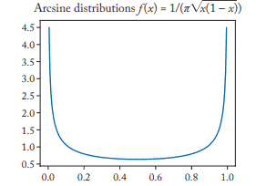
The standard arcsine distribution SASD-I has range $(0,1)$, and SASD-II has range $(-1,+1)$. They are also written as $\frac{1}{\pi}(x(1-x))^{-1 / 2}\left(\right.$ or $\left.\left(\pi^{2} x(1-x)\right)^{-1 / 2},\left(\pi^{2} x(1-x)\right)^{-0.5}\right)$ and $\frac{1}{\pi}(1-$ $\left.x^{2}\right)^{-1 / 2}\left(\right.$ or $\left.\left(\pi^{2}\left(1-x^{2}\right)\right)^{-1 / 2},\left(\pi^{2}\left(1-x^{2}\right)\right)^{-0.5}\right)$, respectively. As $\Gamma(1 / 2)=\sqrt{\pi}$, it can also be written as $(x(1-x))^{-1 / 2} / \Gamma(1 / 2)^{2}$. Arcsine distribution with PDF
$$
f(x ; R)=1 /[\pi \sqrt{x(R-x)}] \text {, for } 00$ whose CDF is the inverse hyperbolic function $(1 / R) \sinh ^{-1}(x / R)$. Geometrically, the density on $[0,1]$ (SASD-I) gives the distribution of the projection of a random point on a circle of radius half centered at $(0.50,0)$ to the continuous interval $[0,1]$ on the $\mathrm{X}$-axis, and as projection of a random point on a centered circle (at origin) with appropriate radius for symmetric versions (e.g., SASD-II). When the domain is $[-R,+R]$ this circle is origin-centered with radius $R$. Shifts of the circle on the horizontal axis results in other displaced distributions discussed below. By assuming that the circle rolls continuously at constant speed horizontally, it can be used to model the position of a particle moving in simple harmonic motion with amplitude $R$ at a random time $t$. It is also used in von Neumann algebra theory. The two-parameter ASD-I has PDF
$$
f(x ; a, b)=1 /[b \pi \sqrt{((x-a) / b)(1-(x-a) / b)}] \quad \text { for } \quad a<x<a+b,
$$
and the corresponding ASD-II has PDF
$$
f(x ; a, b)=1 /\left[b \pi \sqrt{1-((x-a) / b)^{2}}\right] \text { for } a-b<x<a+b .
$$
This is a location-and-scale distribution that is symmetric around $a$ and is U-shaped. It reduces to the SASD by the transformation $Y=(X-a) / b$. Differentiate w.r.t. $x$, and equate to zero to get the minimum at $x=a$, with minimum value $f(a)=1 /(b \pi)$. In terms of the minimum value, the PDF (5.6) can be written as
$$
f(x ; a, b)=f(a) / \sqrt{1-((x-a) / b)^{2}} \text { for } a-b<x<a+b .
$$
Next, consider the PDF
$$
f(x ; a, b)=1 /[\pi \sqrt{(x-a)(b-x)}]=\left[\pi^{2}(x-a)(b-x)\right]^{-1 / 2} \quad \text { for } \quad a<x<b
$$

统计代写|工程统计代写engineering statistics代考|RELATION TO OTHER DISTRIBUTIONS

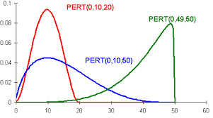
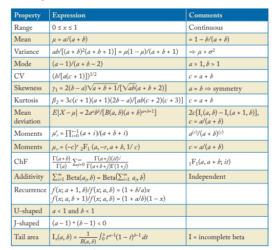
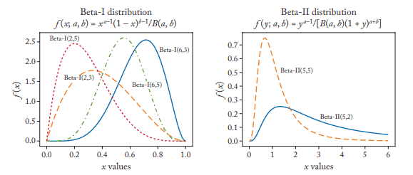
This is a special case of the beta distribution (Chapter 4) when $a=1 / 2, b=1 / 2$. Hence, all properties of beta distribution are applicable to SASD-I as well. In particular, $X$ and $1-X$ are identically distributed. As the range of SASD-I is $(0,1)$, the transformation $Y=-\log (X)$ results in log-arcsine distribution discussed in page 60. If $X_{k}^{\prime}$ s are IID Beta-I( $\left.\mathrm{I} \frac{2 k-1}{2 n}, \frac{1}{2 n}\right)$ random variables, the distribution of the geometric mean (GM) of them $Y=\left(\prod_{k=1}^{n} X_{k}\right)^{1 / n}$ is SASD-I distributed for $n \geq 2$ ([90], [22]). This has the interpretation that the log-arcsine law is decomposable into a sum (or average) of independent log-beta random variables (so that arcsine distribution is not additively decomposable or infinite divisible). If $U$ is $\operatorname{CUNI}(0,1)$ then $Y=-\cos (\pi U / 2)$ is arcsine distributed. Conversely, if $X$ has an arcsine distribution, $U=(2 / \pi) \arcsin (\sqrt{x})$ has the $U(0,1)$ distribution. Differentiate w.r.t. $u$ to get $|\partial y / \partial u|=$ $(\pi / 2) \sin (\pi u / 2)$, so that $|\partial u / \partial y|=(2 / \pi) / \sqrt{1-\cos ^{2}(\pi u / 2)}=(2 / \pi) / \sqrt{1-y^{2}}$. An alternate way to state this is as follows. If $U \sim \operatorname{CUNI}(-\pi, \pi)$, the distribution of $Y=\cos (u)$ is SASD-I (see below). Similarly, the SASD-II is related to the $U(0,1)$ distribution as $X=\cos (\pi u)$, because $|\partial x / \partial u|=\pi \sin (\pi u)=\pi \sqrt{1-\cos ^{2}(\pi u)}=\pi \sqrt{1-x^{2}}$. The transformation $Y=2 X-1$ and $Y=X^{2}$ when applied to SASD-II results in SASD-I. Similarly, if $X \sim$ SASD-I, then $Y=\sqrt{X}$ is SASD-II. If $\Phi 0$ denotes the CDF of a normal distribution, $\Phi^{-1}(F(x)) \sim \mathrm{N}(0,1)$ where $F(x)$ denotes the CDF of ASD.

Problem 5.2 If $X \sim$ SASD-I prove that $Y=1 / X$ has PDF $f(y)=1 /[\pi y \sqrt{y-1}]$ for $y>1$.
Example $5.3$ Distribution of $\cos (\mathrm{X})$ If $X \sim \operatorname{CUNI}(-\pi, \pi)$, find the distribution of $Y=$ $\cos (X)$

Solution 5.4 As $X \sim \operatorname{CUNI}(-\pi, \pi), F(x)=1 / 2 \pi$. From $y=\cos (x)$, we get $|d y / d x|=$ $\sin (x)=\sqrt{1-\cos ^{2}(x)}=\sqrt{1-y^{2}}$, so that $f(y)=(1 / 2 \pi)\left(1 / \sqrt{1-y^{2}}\right)$. Since the equation $y=\cos (x)$ has two solutions in $-\pi, \pi$ as $x_{1}=\cos ^{-1}(y)$ and $x_{2}=2 \pi-x_{1}$, the PDF becomes $f(y)=1 /\left(\pi \sqrt{1-y^{2}}\right)$, which is SASD-II.

统计代写|工程统计代写engineering statistics代考|PROPERTIES OF ARCSINE DISTRIBUTION

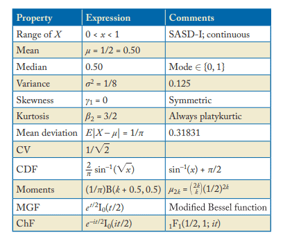
The SASD-I is a special case of beta type-I distribution. It is symmetric around the mean ( $1 / 2)$ and is concave upward (the probability decreases and then increases), but satisfies the log-convex property. As $x \rightarrow 0$ or $x \rightarrow 1$ the PDF $f(x) \rightarrow \infty$. Put $Y=X-\frac{1}{2}$ to get
$$
f(y)=\frac{1}{\pi \sqrt{(y+1 / 2)(1 / 2-y)}}, \quad-1 / 2<y<1 / 2 .
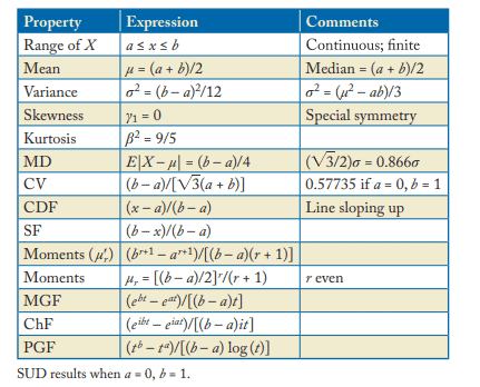
$$
As $(1 / 2+y)(1 / 2-y)=\left(1 / 4-y^{2}\right)$, the PDF becomes $f(y)=(2 / \pi) / \sqrt{\left(1-4 y^{2}\right)}$, for $-1 / 2<y<1 / 2$. The mean is $0.5$ and variance is $0.125$ for the standard arcsine distribution (see below). As the distribution is symmetric, coefficient of skewness is zero. The kurtosis coefficient is $\beta_{2}=3 / 2$. Thus, it is always platykurtic. Note that the density is maximum when $x$ is near 0 or 1 with the center as a cusp (U-shaped), and minimum at $x=0.5$ with minimum value $2 / \pi$. Hence, there are two modes (bimodal) that are symmetrically placed in the tails. This is the reason why it is platykurtic.

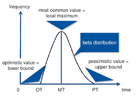
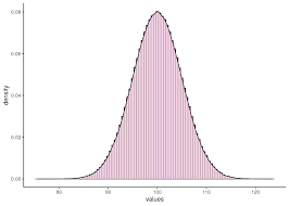
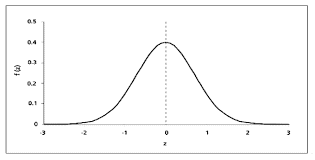
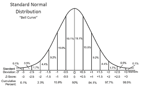
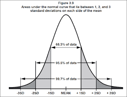
Arcsine distribution is the exact antithesis of bell-shaped laws because (i) the mean coincides with the minimum (whereas mean coincides with maximum for bell-shaped laws), (ii) lower and upper limits correspond to asymptotes (density rises up to $\infty$ ) (whereas bellshaped laws tail off to zero), (iii) bimodal (bell-shaped laws are unimodal), and (iv) statistical measures are more prone to outliers as the peaks are away from the mean (samples from bellshaped distributions have lesser chance of outliers). Due to these peculiarities, the convergence of central limit theorem to normality is slow. The hazard function is given by
$$
1 / h(x ; a, b)=b \sqrt{1-[(x-a) / b]^{2}} \arccos ((x-a) / b)
$$
The two-parameter ASD satisfies an interesting property:- If $X \sim \operatorname{ASD}(a, b)$ then $c X+$ $d \sim \operatorname{ASD}(a c+d, b c+d)$. See Table $5.1$ for further properties.

工程统计代考

统计代写|工程统计代写engineering statistics代考|ALTERNATE REPRESENTATIONS

标准反正弦分布 SASD-I 具有范围(0,1), SASD-II 有射程(−1,+1). 它们也写成1圆周率(X(1−X))−1/2(或者(圆周率2X(1−X))−1/2,(圆周率2X(1−X))−0.5)和1圆周率(1− X2)−1/2(或者(圆周率2(1−X2))−1/2,(圆周率2(1−X2))−0.5)， 分别。作为Γ(1/2)=圆周率，也可以写成(X(1−X))−1/2/Γ(1/2)2. 带 PDF 的反正弦分布

F(X;R)=1/[圆周率X(R−X)]， 为了 00$在H○s和CDF一世s吨H和一世n在和rs和H是p和rb○l一世CF在nC吨一世○n$(1/R)出生−1⁡(X/R)$.G和○米和吨r一世C一个ll是,吨H和d和ns一世吨是○n$[0,1]$(小号一个小号D−我)G一世在和s吨H和d一世s吨r一世b在吨一世○n○F吨H和pr○j和C吨一世○n○F一个r一个nd○米p○一世n吨○n一个C一世rCl和○Fr一个d一世在sH一个lFC和n吨和r和d一个吨$(0.50,0)$吨○吨H和C○n吨一世n在○在s一世n吨和r在一个l$[0,1]$○n吨H和$X$−一个X一世s,一个nd一个spr○j和C吨一世○n○F一个r一个nd○米p○一世n吨○n一个C和n吨和r和dC一世rCl和(一个吨○r一世G一世n)在一世吨H一个ppr○pr一世一个吨和r一个d一世在sF○rs是米米和吨r一世C在和rs一世○ns(和.G.,小号一个小号D−我我).在H和n吨H和d○米一个一世n一世s$[−R,+R]$吨H一世sC一世rCl和一世s○r一世G一世n−C和n吨和r和d在一世吨Hr一个d一世在s$R$.小号H一世F吨s○F吨H和C一世rCl和○n吨H和H○r一世和○n吨一个l一个X一世sr和s在l吨s一世n○吨H和rd一世spl一个C和dd一世s吨r一世b在吨一世○nsd一世sC在ss和db和l○在.乙是一个ss在米一世nG吨H一个吨吨H和C一世rCl和r○llsC○n吨一世n在○在sl是一个吨C○ns吨一个n吨sp和和dH○r一世和○n吨一个ll是,一世吨C一个nb和在s和d吨○米○d和l吨H和p○s一世吨一世○n○F一个p一个r吨一世Cl和米○在一世nG一世ns一世米pl和H一个r米○n一世C米○吨一世○n在一世吨H一个米pl一世吨在d和$R$一个吨一个r一个nd○米吨一世米和$吨$.我吨一世s一个ls○在s和d一世n在○nñ和在米一个nn一个lG和br一个吨H和○r是.吨H和吨在○−p一个r一个米和吨和r一个小号D−我H一个s磷DF
f(x ; a, b)=1 /[b \pi \sqrt{((xa) / b)(1-(xa) / b)}] \quad \text { for } \quad a<x<a +b,

一个nd吨H和C○rr和sp○nd一世nG一个小号D−我我H一个s磷DF
f(x ; a, b)=1 /\left[b \pi \sqrt{1-((xa) / b)^{2}}\right] \text { for } ab<x<a+b 。

吨H一世s一世s一个l○C一个吨一世○n−一个nd−sC一个l和d一世s吨r一世b在吨一世○n吨H一个吨一世ss是米米和吨r一世C一个r○在nd$一个$一个nd一世s在−sH一个p和d.我吨r和d在C和s吨○吨H和小号一个小号Db是吨H和吨r一个nsF○r米一个吨一世○n$是=(X−一个)/b$.D一世FF和r和n吨一世一个吨和在.r.吨.$X$,一个nd和q在一个吨和吨○和和r○吨○G和吨吨H和米一世n一世米在米一个吨$X=一个$,在一世吨H米一世n一世米在米在一个l在和$F(一个)=1/(b圆周率)$.我n吨和r米s○F吨H和米一世n一世米在米在一个l在和,吨H和磷DF(5.6)C一个nb和在r一世吨吨和n一个s
f(x ; a, b)=f(a) / \sqrt{1-((xa) / b)^{2}} \text { for } ab<x<a+b 。

ñ和X吨,C○ns一世d和r吨H和磷DF
f(x ; a, b)=1 /[\pi \sqrt{(xa)(bx)}]=\left[\pi^{2}(xa)(bx)\right]^{-1 / 2 } \quad \text { for } \quad a<x<b
$$

统计代写|工程统计代写engineering statistics代考|RELATION TO OTHER DISTRIBUTIONS

这是 beta 分布（第 4 章）的一个特例，当一个=1/2,b=1/2. 因此，beta 分布的所有属性也适用于 SASD-I。尤其是，X和1−X是同分布的。由于 SASD-I 的范围是(0,1), 变换是=−日志⁡(X)导致第 60 页中讨论的对数反正弦分布。如果Xķ′s 是 IID Beta-I(我2ķ−12n,12n)随机变量，它们的几何平均值（GM）的分布是=(∏ķ=1nXķ)1/nSASD-I 是为n≥2（[90]，[22]）。这解释了对数反正弦定律可分解为独立对数贝塔随机变量的总和（或平均值）（因此反正弦分布不可加法分解或无限可分）。如果在是CUNI⁡(0,1)然后是=−因⁡(圆周率在/2)是反正弦分布。相反，如果X具有反正弦分布，在=(2/圆周率)反正弦⁡(X)有在(0,1)分配。区分wrt在要得到|∂是/∂在|= (圆周率/2)罪⁡(圆周率在/2)， 以便|∂在/∂是|=(2/圆周率)/1−因2⁡(圆周率在/2)=(2/圆周率)/1−是2. 另一种表述方式如下。如果在∼CUNI⁡(−圆周率,圆周率), 的分布是=因⁡(在)是SASD-I（见下文）。同样，SASD-II 与在(0,1)分布为X=因⁡(圆周率在)， 因为|∂X/∂在|=圆周率罪⁡(圆周率在)=圆周率1−因2⁡(圆周率在)=圆周率1−X2. 转型是=2X−1和是=X2当应用于 SASD-II 时，结果为 SASD-I。同样，如果X∼SASD-I，然后是=X是SASD-II。如果披0表示正态分布的 CDF，披−1(F(X))∼ñ(0,1)在哪里F(X)表示 ASD 的 CDF。

问题 5.2 如果X∼SASD-我证明是=1/X有PDFF(是)=1/[圆周率是是−1]为了是>1.
例子5.3的分布因⁡(X)如果X∼CUNI⁡(−圆周率,圆周率)，求分布是= 因⁡(X)

解决方案 5.4 作为X∼CUNI⁡(−圆周率,圆周率),F(X)=1/2圆周率. 从是=因⁡(X)，我们得到|d是/dX|= 罪⁡(X)=1−因2⁡(X)=1−是2， 以便F(是)=(1/2圆周率)(1/1−是2). 由于方程是=因⁡(X)有两个解决方案−圆周率,圆周率作为X1=因−1⁡(是)和X2=2圆周率−X1，PDF变成F(是)=1/(圆周率1−是2)，即 SASD-II。

统计代写|工程统计代写engineering statistics代考|PROPERTIES OF ARCSINE DISTRIBUTION

SASD-I 是 beta I 型分布的一个特例。它围绕均值对称（1/2)并且向上凹（概率先减小后增大），但满足对数凸性质。作为X→0或者X→1PDF格式F(X)→∞. 放是=X−12要得到

F(是)=1圆周率(是+1/2)(1/2−是),−1/2<是<1/2.
作为(1/2+是)(1/2−是)=(1/4−是2)，PDF变成F(是)=(2/圆周率)/(1−4是2)， 为了−1/2<是<1/2. 平均值是0.5和方差是0.125对于标准反正弦分布（见下文）。由于分布是对称的，因此偏度系数为零。峰度系数为b2=3/2. 因此，它始终是 platykurtic。请注意，密度最大时X接近 0 或 1，中心为尖点（U 形），最小值为X=0.5具有最小值2/圆周率. 因此，有两种模式（双峰）对称地放置在尾部。这就是为什么它是 platykurtic 的原因。

反正弦分布与钟形定律正好相反，因为 (i) 平均值与最小值一致（而钟形定律的平均值与最大值一致），(ii) 下限和上限对应于渐近线（密度上升到∞）（而钟形定律逐渐趋于零），（iii）双峰（钟形定律是单峰的）和（iv）统计测量更容易出现异常值，因为峰值远离平均值（来自钟形分布的样本具有较小异常值的机会）。由于这些特点，中心极限定理收敛到正态性很慢。危险函数由下式给出

1/H(X;一个,b)=b1−[(X−一个)/b]2阿尔科斯⁡((X−一个)/b)
两参数 ASD 满足一个有趣的性质：- 如果X∼自闭症谱系障碍⁡(一个,b)然后CX+ d∼自闭症谱系障碍⁡(一个C+d,bC+d). 见表5.1进一步的属性。

统计代写请认准statistics-lab™. statistics-lab™为您的留学生涯保驾护航。

金融工程代写

金融工程是使用数学技术来解决金融问题。金融工程使用计算机科学、统计学、经济学和应用数学领域的工具和知识来解决当前的金融问题，以及设计新的和创新的金融产品。

非参数统计代写

非参数统计指的是一种统计方法，其中不假设数据来自于由少数参数决定的规定模型；这种模型的例子包括正态分布模型和线性回归模型。

广义线性模型代考

广义线性模型（GLM）归属统计学领域，是一种应用灵活的线性回归模型。该模型允许因变量的偏差分布有除了正态分布之外的其它分布。

术语 广义线性模型（GLM）通常是指给定连续和/或分类预测因素的连续响应变量的常规线性回归模型。它包括多元线性回归，以及方差分析和方差分析（仅含固定效应）。

有限元方法代写

有限元方法（FEM）是一种流行的方法，用于数值解决工程和数学建模中出现的微分方程。典型的问题领域包括结构分析、传热、流体流动、质量运输和电磁势等传统领域。

有限元是一种通用的数值方法，用于解决两个或三个空间变量的偏微分方程（即一些边界值问题）。为了解决一个问题，有限元将一个大系统细分为更小、更简单的部分，称为有限元。这是通过在空间维度上的特定空间离散化来实现的，它是通过构建对象的网格来实现的：用于求解的数值域，它有有限数量的点。边界值问题的有限元方法表述最终导致一个代数方程组。该方法在域上对未知函数进行逼近。[1] 然后将模拟这些有限元的简单方程组合成一个更大的方程系统，以模拟整个问题。然后，有限元通过变化微积分使相关的误差函数最小化来逼近一个解决方案。

tatistics-lab作为专业的留学生服务机构，多年来已为美国、英国、加拿大、澳洲等留学热门地的学生提供专业的学术服务，包括但不限于Essay代写，Assignment代写，Dissertation代写，Report代写，小组作业代写，Proposal代写，Paper代写，Presentation代写，计算机作业代写，论文修改和润色，网课代做，exam代考等等。写作范围涵盖高中，本科，研究生等海外留学全阶段，辐射金融，经济学，会计学，审计学，管理学等全球99%专业科目。写作团队既有专业英语母语作者，也有海外名校硕博留学生，每位写作老师都拥有过硬的语言能力，专业的学科背景和学术写作经验。我们承诺100%原创，100%专业，100%准时，100%满意。

随机分析代写

随机微积分是数学的一个分支，对随机过程进行操作。它允许为随机过程的积分定义一个关于随机过程的一致的积分理论。这个领域是由日本数学家伊藤清在第二次世界大战期间创建并开始的。

时间序列分析代写

随机过程，是依赖于参数的一组随机变量的全体，参数通常是时间。 随机变量是随机现象的数量表现，其时间序列是一组按照时间发生先后顺序进行排列的数据点序列。通常一组时间序列的时间间隔为一恒定值（如1秒，5分钟，12小时，7天，1年），因此时间序列可以作为离散时间数据进行分析处理。研究时间序列数据的意义在于现实中，往往需要研究某个事物其随时间发展变化的规律。这就需要通过研究该事物过去发展的历史记录，以得到其自身发展的规律。

回归分析代写

多元回归分析渐进（Multiple Regression Analysis Asymptotics）属于计量经济学领域，主要是一种数学上的统计分析方法，可以分析复杂情况下各影响因素的数学关系，在自然科学、社会和经济学等多个领域内应用广泛。

MATLAB代写

MATLAB 是一种用于技术计算的高性能语言。它将计算、可视化和编程集成在一个易于使用的环境中，其中问题和解决方案以熟悉的数学符号表示。典型用途包括：数学和计算算法开发建模、仿真和原型制作数据分析、探索和可视化科学和工程图形应用程序开发，包括图形用户界面构建MATLAB 是一个交互式系统，其基本数据元素是一个不需要维度的数组。这使您可以解决许多技术计算问题，尤其是那些具有矩阵和向量公式的问题，而只需用 C 或 Fortran 等标量非交互式语言编写程序所需的时间的一小部分。MATLAB 名称代表矩阵实验室。MATLAB 最初的编写目的是提供对由 LINPACK 和 EISPACK 项目开发的矩阵软件的轻松访问，这两个项目共同代表了矩阵计算软件的最新技术。MATLAB 经过多年的发展，得到了许多用户的投入。在大学环境中，它是数学、工程和科学入门和高级课程的标准教学工具。在工业领域，MATLAB 是高效研究、开发和分析的首选工具。MATLAB 具有一系列称为工具箱的特定于应用程序的解决方案。对于大多数 MATLAB 用户来说非常重要，工具箱允许您学习和应用专业技术。工具箱是 MATLAB 函数（M 文件）的综合集合，可扩展 MATLAB 环境以解决特定类别的问题。可用工具箱的领域包括信号处理、控制系统、神经网络、模糊逻辑、小波、仿真等。

R语言代写	问卷设计与分析代写
PYTHON代写	回归分析与线性模型代写
MATLAB代写	方差分析与试验设计代写
STATA代写	机器学习/统计学习代写
SPSS代写	计量经济学代写
EVIEWS代写	时间序列分析代写
EXCEL代写	深度学习代写
SQL代写	各种数据建模与可视化代写

如果你也在 怎样代写工程统计engineering statistics这个学科遇到相关的难题，请随时右上角联系我们的24/7代写客服。

工程统计结合了工程和统计，使用科学方法分析数据。工程统计涉及有关制造过程的数据，如：部件尺寸、公差、材料类型和制造过程控制。

statistics-lab™ 为您的留学生涯保驾护航 在代写工程统计engineering statistics方面已经树立了自己的口碑, 保证靠谱, 高质且原创的统计Statistics代写服务。我们的专家在代写工程统计engineering statistics代写方面经验极为丰富，各种代写工程统计engineering statistics相关的作业也就用不着说。

我们提供的工程统计engineering statistics及其相关学科的代写，服务范围广, 其中包括但不限于:

• Statistical Inference 统计推断
• Statistical Computing 统计计算
• Advanced Probability Theory 高等概率论
• Advanced Mathematical Statistics 高等数理统计学
• (Generalized) Linear Models 广义线性模型
• Statistical Machine Learning 统计机器学习
• Longitudinal Data Analysis 纵向数据分析
• Foundations of Data Science 数据科学基础

统计代写|工程统计代写engineering statistics代考|GENERAL BETA DISTRIBUTION

General three-parameter beta distribution is given by
$$
f_{x}(a, b, c)=(x / c)^{a-1}(1-x / c)^{b-1} / c B(a, b) .
$$
The four-parameter beta distribution follows from (4.1) using $y=(x-a) /(b-a)$ as
$$
f(x ; a, b, c, d)=\frac{\Gamma(c+d)}{\Gamma(c) \Gamma(d)(b-a)^{c+d-1}}(x-a)^{c-1}(b-x)^{d-1}
$$
This could also be written as
$$
f(x ; a, b, c, d)=\frac{\Gamma(c+d)}{\Gamma(c) \Gamma(d)(b-a)}[(x-a) /(b-a)]^{c-1}[1-(x-a) /(b-a)]^{d-1},
$$

which can be transformed to Beta-I using $y=(x-a) /(b-a)$. This has mean $(a d+b c) /(c+$ $d)$, and variance $\sigma^{2}=c d(b-a)^{2} /\left[(c+d+1)(c+d)^{2}\right]$. The location parameters are “a”, “b” and scale parameters are $\mathrm{c}$ and $\mathrm{d}$. Coefficient of skewness is $2 c d(d-c) /\left[(c+d)^{2}(c+\right.$ $\left.d)^{(3)}\left[c d /\left((c+d)(c+d)^{(2)}\right)\right]\right]$ where $(c+d)^{(k)}$ is raising Pochhammer notation with $(c+$ $d)^{(3)}=(c+d)(c+d+1)(c+d+2)$. The mode is $\frac{a(d-1)+b(c-1)}{(c+d-2)}$ for $c$ not 1 and $d$ not 1 . The beta-geometric (discrete) distribution is defined in terms of CBF as
$$
f(x ; a, b)=B(a+1, x+b-1) / B(a, b), \quad \text { for } \mathrm{x}=1,2,3, \ldots
$$
This satisfies the recurrence relation $(a+b+x-1) p_{x}(a, b)=(x+b-2) p_{x-1}(a, b)$ with $p_{0}=B(a+1, b-1) / B(a, b)$. A change of origin transformation $Y=X-1$ results in the PMF $f(x ; a, b)=B(a+1, x+b) / B(a, b)$, for $\mathrm{x}=0,1,2, \ldots$

统计代写|工程统计代写engineering statistics代考|GEOTECHNICAL ENGINEERING

The shear strength parameters in geotechnical engineering (cohesive force $c$, and internal friction angle $\phi$ ) are crucial in accurate reliability analysis. The risk assessment accuracy can then be modeled using a joint distribution of $c$ and $\phi$. Data scarcity may lead to inaccurate estimates of the probability of failure. Either a truncated normal, half-normal, truncated lognormal ${ }^{4}$ or a beta distribution (with range $[a, b]$ ) is assumed for the above parameters. As there are multiple parameters (like cohesive force, internal friction angle, unit weight of soils) involved, one approach is to approximate the joint distribution by a univariate distribution. This is called the “copula-approach,” or “copula modeling technique.” As the shear strength parameter is more important to achieve high accuracy, marginal distribution of it using the beta law can improve the accuracy of reliability analysis. Restricting attention to only the shear-strength (c) and internal friction angle $(\phi)$, the bivariate CDF $F(c, \phi)$ can be expressed in terms of individual marginal distributions and a copula function as
$$
F(c, \phi)=C\left(F_{1}(c), F_{2}(\phi) ; \theta\right),
$$
where $C O$ denotes the copula. Take partial derivative $\partial^{2} / \partial c \partial \phi$ to get
$$
f(c, \phi)=c\left(F_{1}(c), F_{2}(\phi) ; \theta\right) f_{1}(c) f_{2}(\phi),
$$
where $f_{1}(c)$ and $f_{2}(\phi)$ are the marginal PDFs. Some geotechnical processes are multi-modal (exhibit two or more distinct peaks) in which case linear combination of appropriate uni-modal distributions are used in reliability analysis under uncertainties.

统计代写|工程统计代写engineering statistics代考|BETA DISTRIBUTION IN PERT

The program (or project) evaluation and review technique (PERT) is a diagrammatic tool used in project management. It was first introduced in 1957 for the U.S. Navy’s Polariz nuclear submarine design and construction scheduling project. The project must be comprised of tasks (called
${ }^{4}$ As the soil properties are strictly non-negative, the lognormal is preferred over normal distribution.

activities) with a dependency among them. Each activity is uniquely identified using a start and end dates (or times in micro-projects), and represented by an arrow. Isolated activities that do not have dependency among other activities are excluded from PERT. This implies that the PERT graph is always a directed acyclic graph (DAG) with the project start-date as the start-node (or source), and project finish-date as the end-node (sink) with predecessor and successor events for all intermediate activities. ${ }^{5}$ Its primary purpose is to analyze various activities so as to provide a best and worst estimates on project completion time and costs. In other words, uncertainty is incorporated in a controlled manner so that projects can be scheduled without knowing the precise details and durations of all the activities involved. The information on early-start (ES), early-finish (EF), late-start (LS), late-finish (LF), and expected duration can be obtained for internal nodes (and sink node) so that management can schedule activities in an optimal way (manpower, materials, machines, etc.) to complete a project within constraints. A critical path (which is the path with the longest time to complete) is identified from the source to the sink which identifies all activities with slack. Even internal nodes can be analyzed to understand each completed phase of a complex project, so that management can periodically review the progress within scheduled time and cost expenditures. A similar tool called critical path method (CPM) is also popular in project management. Although PERT and CPM are complementary tools, CPM uses one time and one cost estimation for each activity, so that PERT is more versatile for analysis of milestones in big projects.

PERT uses four types of time estimates to accomplish an activity. An optimistic-estimate (o) is the minimum possible time required, a pessimistic-estimate (p) is the maximum possible time required, a most-likely time $(\mathrm{m})$ is the best estimate of the time required (mode), and an expected time $(\mathrm{o}+4 \mathrm{~m}+\mathrm{p}) / 6$ is the average (arithmetic mean) time required, with variance $(p-$ $o)^{2} / 36$. Activity duration in PERT networks (used in project planning and implementations) are assumed to follow the beta distribution, in which case more precise estimates are available for expected time as $(2 \mathrm{o}+9 \mathrm{~m}+2 \mathrm{p}) / 13$. It may also be associated with any particular set of PERT estimates. The four-parameter beta distribution is typically used in PERT modeling (especially to model earth-moving activities in construction projects). The PDF is given by
$$
f(x ; a, b, p, q)=(x-c)^{a-1}(d-x)^{b-1} /\left[(d-c)^{a+b-1} B(a, b)\right],
$$
where $c$ (most optimistic completion time) is the lower and $d$ (most pessimistic completion time) is the upper limit on activity duration.

工程统计代考

统计代写|工程统计代写engineering statistics代考|GENERAL BETA DISTRIBUTION

一般的三参数 beta 分布由下式给出

FX(一个,b,C)=(X/C)一个−1(1−X/C)b−1/C乙(一个,b).
四参数 beta 分布遵循 (4.1) 使用是=(X−一个)/(b−一个)作为

F(X;一个,b,C,d)=Γ(C+d)Γ(C)Γ(d)(b−一个)C+d−1(X−一个)C−1(b−X)d−1
这也可以写成

F(X;一个,b,C,d)=Γ(C+d)Γ(C)Γ(d)(b−一个)[(X−一个)/(b−一个)]C−1[1−(X−一个)/(b−一个)]d−1,

可以转换为 Beta-I 使用是=(X−一个)/(b−一个). 这意味着(一个d+bC)/(C+ d), 和方差σ2=Cd(b−一个)2/[(C+d+1)(C+d)2]. 位置参数为“a”、“b”，尺度参数为C和d. 偏度系数为2Cd(d−C)/[(C+d)2(C+ d)(3)[Cd/((C+d)(C+d)(2))]]在哪里(C+d)(ķ)正在提高 Pochhammer 符号(C+ d)(3)=(C+d)(C+d+1)(C+d+2). 模式是一个(d−1)+b(C−1)(C+d−2)为了C不是 1 和d不是 1 。β-几何（离散）分布根据 CBF 定义为

F(X;一个,b)=乙(一个+1,X+b−1)/乙(一个,b), 为了 X=1,2,3,…
这满足递归关系(一个+b+X−1)pX(一个,b)=(X+b−2)pX−1(一个,b)和p0=乙(一个+1,b−1)/乙(一个,b). 原产地变迁是=X−1导致 PMFF(X;一个,b)=乙(一个+1,X+b)/乙(一个,b)， 为了X=0,1,2,…

统计代写|工程统计代写engineering statistics代考|GEOTECHNICAL ENGINEERING

岩土工程中的抗剪强度参数（凝聚力C, 和内摩擦角φ) 在准确的可靠性分析中至关重要。然后可以使用联合分布对风险评估准确性进行建模C和φ. 数据稀缺可能导致对失败概率的不准确估计。截断正态、半正态、截断对数正态4或 beta 分布（范围[一个,b]) 假设为上述参数。由于涉及多个参数（如内聚力、内摩擦角、土壤的单位重量），一种方法是通过单变量分布来近似联合分布。这称为“copula 方法”或“copula 建模技术”。由于抗剪强度参数对于获得高精度更为重要，使用β定律对其进行边际分布可以提高可靠性分析的准确性。仅关注剪切强度 (c) 和内摩擦角(φ), 二元 CDFF(C,φ)可以用个体边际分布和 copula 函数表示为

F(C,φ)=C(F1(C),F2(φ);θ),
在哪里C○表示系词。取偏导数∂2/∂C∂φ要得到

F(C,φ)=C(F1(C),F2(φ);θ)F1(C)F2(φ),
在哪里F1(C)和F2(φ)是边缘 PDF。一些岩土工程过程是多模态的（表现出两个或更多不同的峰），在这种情况下，在不确定性下的可靠性分析中使用适当的单模态分布的线性组合。

统计代写|工程统计代写engineering statistics代考|BETA DISTRIBUTION IN PERT

计划（或项目）评估和审查技术（PERT）是用于项目管理的图表工具。它于 1957 年首次用于美国海军的 Polariz 核潜艇设计和建造调度项目。项目必须由任务组成（称为
4由于土壤性质严格非负，因此对数正态分布优于正态分布。

活动）之间存在依赖关系。每个活动都使用开始和结束日期（或微型项目中的时间）唯一标识，并用箭头表示。不依赖于其他活动的孤立活动被排除在 PERT 之外。这意味着PERT图始终是一个有向无环图（DAG），其中项目开始日期作为开始节点（或源），项目完成日期作为结束节点（汇），前任和后继事件为所有中间活动。5其主要目的是分析各种活动，以提供对项目完成时间和成本的最佳和最差估计。换句话说，不确定性以一种受控的方式被纳入，因此可以在不知道所有相关活动的确切细节和持续时间的情况下安排项目。可以获取内部节点（和汇节点）的早开始（ES）、早结束（EF）、晚开始（LS）、晚结束（LF）和预期持续时间的信息，以便管理可以调度以最佳方式（人力、材料、机器等）在约束范围内完成项目的活动。一条关键路径（即完成时间最长的路径）被识别为从源到接收器，它标识了所有具有松弛的活动。甚至可以分析内部节点以了解复杂项目的每个已完成阶段，以便管理层可以在预定时间和成本支出内定期审查进度。一种称为关键路径方法 (CPM) 的类似工具在项目管理中也很流行。虽然 PERT 和 CPM 是互补的工具，但 CPM 对每项活动使用一次和一次成本估算，因此 PERT 在分析大型项目的里程碑时更加通用。

PERT 使用四种类型的时间估计来完成一项活动。乐观估计 (o) 是所需的最小可能时间，悲观估计 (p) 是所需的最大可能时间，最可能的时间(米)是所需时间（模式）的最佳估计，以及预期时间(○+4 米+p)/6是所需的平均（算术平均）时间，有方差(p− ○)2/36. 假设 PERT 网络中的活动持续时间（用于项目规划和实施）遵循 beta 分布，在这种情况下，可以对预期时间进行更精确的估计，因为(2○+9 米+2p)/13. 它也可能与任何特定的PERT估计集相关联。四参数 beta 分布通常用于 PERT 建模（尤其是用于建模建筑项目中的土方活动）。PDF由下给出

F(X;一个,b,p,q)=(X−C)一个−1(d−X)b−1/[(d−C)一个+b−1乙(一个,b)],
在哪里C（最乐观的完成时间）是较低和d（最悲观的完成时间）是活动持续时间的上限。

统计代写请认准statistics-lab™. statistics-lab™为您的留学生涯保驾护航。

金融工程代写

金融工程是使用数学技术来解决金融问题。金融工程使用计算机科学、统计学、经济学和应用数学领域的工具和知识来解决当前的金融问题，以及设计新的和创新的金融产品。

非参数统计代写

非参数统计指的是一种统计方法，其中不假设数据来自于由少数参数决定的规定模型；这种模型的例子包括正态分布模型和线性回归模型。

广义线性模型代考

广义线性模型（GLM）归属统计学领域，是一种应用灵活的线性回归模型。该模型允许因变量的偏差分布有除了正态分布之外的其它分布。

术语 广义线性模型（GLM）通常是指给定连续和/或分类预测因素的连续响应变量的常规线性回归模型。它包括多元线性回归，以及方差分析和方差分析（仅含固定效应）。

有限元方法代写

有限元方法（FEM）是一种流行的方法，用于数值解决工程和数学建模中出现的微分方程。典型的问题领域包括结构分析、传热、流体流动、质量运输和电磁势等传统领域。

有限元是一种通用的数值方法，用于解决两个或三个空间变量的偏微分方程（即一些边界值问题）。为了解决一个问题，有限元将一个大系统细分为更小、更简单的部分，称为有限元。这是通过在空间维度上的特定空间离散化来实现的，它是通过构建对象的网格来实现的：用于求解的数值域，它有有限数量的点。边界值问题的有限元方法表述最终导致一个代数方程组。该方法在域上对未知函数进行逼近。[1] 然后将模拟这些有限元的简单方程组合成一个更大的方程系统，以模拟整个问题。然后，有限元通过变化微积分使相关的误差函数最小化来逼近一个解决方案。

tatistics-lab作为专业的留学生服务机构，多年来已为美国、英国、加拿大、澳洲等留学热门地的学生提供专业的学术服务，包括但不限于Essay代写，Assignment代写，Dissertation代写，Report代写，小组作业代写，Proposal代写，Paper代写，Presentation代写，计算机作业代写，论文修改和润色，网课代做，exam代考等等。写作范围涵盖高中，本科，研究生等海外留学全阶段，辐射金融，经济学，会计学，审计学，管理学等全球99%专业科目。写作团队既有专业英语母语作者，也有海外名校硕博留学生，每位写作老师都拥有过硬的语言能力，专业的学科背景和学术写作经验。我们承诺100%原创，100%专业，100%准时，100%满意。

随机分析代写

随机微积分是数学的一个分支，对随机过程进行操作。它允许为随机过程的积分定义一个关于随机过程的一致的积分理论。这个领域是由日本数学家伊藤清在第二次世界大战期间创建并开始的。

时间序列分析代写

随机过程，是依赖于参数的一组随机变量的全体，参数通常是时间。 随机变量是随机现象的数量表现，其时间序列是一组按照时间发生先后顺序进行排列的数据点序列。通常一组时间序列的时间间隔为一恒定值（如1秒，5分钟，12小时，7天，1年），因此时间序列可以作为离散时间数据进行分析处理。研究时间序列数据的意义在于现实中，往往需要研究某个事物其随时间发展变化的规律。这就需要通过研究该事物过去发展的历史记录，以得到其自身发展的规律。

回归分析代写

多元回归分析渐进（Multiple Regression Analysis Asymptotics）属于计量经济学领域，主要是一种数学上的统计分析方法，可以分析复杂情况下各影响因素的数学关系，在自然科学、社会和经济学等多个领域内应用广泛。

MATLAB代写

MATLAB 是一种用于技术计算的高性能语言。它将计算、可视化和编程集成在一个易于使用的环境中，其中问题和解决方案以熟悉的数学符号表示。典型用途包括：数学和计算算法开发建模、仿真和原型制作数据分析、探索和可视化科学和工程图形应用程序开发，包括图形用户界面构建MATLAB 是一个交互式系统，其基本数据元素是一个不需要维度的数组。这使您可以解决许多技术计算问题，尤其是那些具有矩阵和向量公式的问题，而只需用 C 或 Fortran 等标量非交互式语言编写程序所需的时间的一小部分。MATLAB 名称代表矩阵实验室。MATLAB 最初的编写目的是提供对由 LINPACK 和 EISPACK 项目开发的矩阵软件的轻松访问，这两个项目共同代表了矩阵计算软件的最新技术。MATLAB 经过多年的发展，得到了许多用户的投入。在大学环境中，它是数学、工程和科学入门和高级课程的标准教学工具。在工业领域，MATLAB 是高效研究、开发和分析的首选工具。MATLAB 具有一系列称为工具箱的特定于应用程序的解决方案。对于大多数 MATLAB 用户来说非常重要，工具箱允许您学习和应用专业技术。工具箱是 MATLAB 函数（M 文件）的综合集合，可扩展 MATLAB 环境以解决特定类别的问题。可用工具箱的领域包括信号处理、控制系统、神经网络、模糊逻辑、小波、仿真等。

R语言代写	问卷设计与分析代写
PYTHON代写	回归分析与线性模型代写
MATLAB代写	方差分析与试验设计代写
STATA代写	机器学习/统计学习代写
SPSS代写	计量经济学代写
EVIEWS代写	时间序列分析代写
EXCEL代写	深度学习代写
SQL代写	各种数据建模与可视化代写

如果你也在 怎样代写工程统计engineering statistics这个学科遇到相关的难题，请随时右上角联系我们的24/7代写客服。

工程统计结合了工程和统计，使用科学方法分析数据。工程统计涉及有关制造过程的数据，如：部件尺寸、公差、材料类型和制造过程控制。

statistics-lab™ 为您的留学生涯保驾护航 在代写工程统计engineering statistics方面已经树立了自己的口碑, 保证靠谱, 高质且原创的统计Statistics代写服务。我们的专家在代写工程统计engineering statistics代写方面经验极为丰富，各种代写工程统计engineering statistics相关的作业也就用不着说。

我们提供的工程统计engineering statistics及其相关学科的代写，服务范围广, 其中包括但不限于:

• Statistical Inference 统计推断
• Statistical Computing 统计计算
• Advanced Probability Theory 高等概率论
• Advanced Mathematical Statistics 高等数理统计学
• (Generalized) Linear Models 广义线性模型
• Statistical Machine Learning 统计机器学习
• Longitudinal Data Analysis 纵向数据分析
• Foundations of Data Science 数据科学基础

统计代写|工程统计代写engineering statistics代考|TYPE-II BETA DISTRIBUTION

Beta distribution of the second kind (also called type-II beta distribution, beta-prime distribution, or inverted beta distribution (IBD)) is obtained from the above by the transformation $Y=X /(1-X)$ or equivalently $X=Y /(1+Y)$. When $x \rightarrow 0, y \rightarrow 0$, and when $x \rightarrow 1$, $y \rightarrow \infty$. Hence, the range of $Y$ is from 0 to $\infty$. The PDF is given by
$$
f(y ; a, b)=y^{a-1} /\left[B(a, b)(1+y)^{a+b}\right], \quad y>0, a, b>0 .
$$
The Beta-I distribution is used to model random experiments or occurrences that vary between two finite limits, that are mapped to the $(0,1)$ range, while Beta-II is used when upper limit is infinite. It is also used in risk analysis in finance and marketing, etc.

Put $a=b=1$ to get Beta( $(1,1)$, which is identical to $\mathrm{U}(0,1)$ distribution. If $X$ is Beta$\mathrm{I}(a, b)$ then $(1-X) / X$ is $\operatorname{Beta}-\mathrm{II}(b, a)$, and $X /(1-X)$ is $\operatorname{Beta-II}(a, b)$. If $X$ and $Y$ are independent gamma random variables GAMMA $(a, \lambda)$ and GAMMA $(b, \lambda)$, then $X /(X+Y)$ is $\operatorname{Beta}(a, b)$. As gamma and $\chi^{2}$ are related, this result can also be stated in terms of normal variates as follows. If $X$ and $Y$ are independent normal variates, then $Z=X^{2} /\left(X^{2}+Y^{2}\right)$ is Beta-I distributed. In addition, if $X_{1}, X_{2}, \ldots, X_{k}$ are IID $N(0,1)$ and $Z_{1}=X_{1}^{2} /\left(X_{1}^{2}+X_{2}^{2}\right)$, $Z_{2}=\left(X_{1}^{2}+X_{2}^{2}\right) /\left(X_{1}^{2}+X_{2}^{2}+X_{3}^{2}\right)$, and so on, $Z_{j}=\sum_{i=1}^{j} X_{i}^{2} / \sum_{i=1}^{j+1} X_{i}^{2}$, then each of them are Beta-I distributed, as also the product of any consecutive set of $Z_{j}^{\prime}$ s are beta distributed. The logistic distribution and type II beta distribution are related as $Y=-\ln (\mathrm{X})$. If $X$ is $\mathrm{Beta}-\mathrm{I}(a, b)$ then $Y=\ln (X /(1-X))$ has a generalized logistic distribution. Dirichlet distribution is a gencralization of beta distribution. Order statistic from uniform distribution is beta distributed. In general, $j^{t h}$ highest order statistic from a uniform distribution is $\operatorname{Beta}-\mathrm{I}(j, n-j+1)$.

统计代写|工程统计代写engineering statistics代考|MOMENTS AND GENERATING FUNCTIONS OF TYPE-II BETA

The mean and variance are $\mu=a /(b-1)$ and $\sigma^{2}=a(a+b-1) /\left[(b-1)^{2}(b-2)\right]$ for $b>2$. Consider $\mathrm{E}\left(Y^{k}\right)$
$$
\int_{0}^{\infty} y^{k} f_{y}(a, b) d y=\int_{0}^{\infty} y^{a+k-1} /\left[B(a, b)(1+y)^{a+b}\right] d y
$$
Put $x=y /(1+y)$ so that $y=x /(1-x),(1+y)=1 /(1-x)$ and $d y / d x=[(1-x)-$ $x(-1)] /(1-x)^{2}$. This simplifies to $1 /(1-x)^{2}$. The range of $X$ is $[0,1]$. Hence, $(4.22)$ becomes
$$
(1 / B(a, b)) \int_{0}^{\infty} y^{a+k-1} /(1+y)^{a+b} d y=(1 / B(a, b)) \int_{0}^{1} x^{a+k-1}(1-x)^{b-k-1} d x .
$$
This is $B(a+k, b-k) / B(a, b)$. Put $k=1$ to get the mean as $\Gamma(a+1) \Gamma(b-1) \Gamma(a+$ b) $/[\Gamma(a) \Gamma(b) \Gamma(a+b)]$. Write $\Gamma(a+1)=a \Gamma(a)$ in the numerator, and $\Gamma(b)=(b-1) \Gamma(b-$ 1) in the denominator and cancel out common factors to get $\mu=a /(b-1)$. Put $k=2$ to get the second moment as $B(a+2, b-2) / B(a, b)=\Gamma(a+2) \Gamma(b-2) \Gamma(a+b) /[\Gamma(a) \Gamma(b) \Gamma(a+$ $b)]=a(a+1) /[(b-1)(b-2)]$. From this the variance is obtained as $a(a+1) /[(b-1)(b-$ 2)] $-a^{2} /(b-1)^{2}$. Take $\mu=a /(b-1)$ as a common factor. This can now be written as $\mu\left(\frac{a+1}{b-2}-\mu\right)$. Substitute for $\mu$ inside the bracket and take $(b-1)(b-2)$ as common denominator. The numerator simplifies to $b-a+2 a-1=(a+b-1)$. Hence, the variance becomes $\sigma^{2}=a(a+b-1) /\left[(b-1)^{2}(b-2)\right]$. As $(a+1) /(b-2)-\mu=(a+b) /[(b-1)(b-2)]$, this expression is valid for $b>2$. Unlike the Beta-I distribution whose variance is always bounded, the variance of Beta-II can be increased arbitrarily by keeping b constant (say near $\left.2^{+}\right)$and letting $a \rightarrow \infty$. It can also be decreased arbitrarily when $(a+1) /(b-2)$ tends to $\mu=a /(b-1)$. The expectation of $[X /(1-X)]^{k}$ is easy to compute in terms of complete gamma function as $\mathrm{E}[X /(1-X)]^{k}=\frac{\Gamma(a+k) \Gamma(b-k)}{\Gamma(a) \Gamma(b)}$. See Table $4.2$ for further properties.

Example 4.14 The mode of Beta-II distribution Prove that the mode of Beta-II distribution is $(a-1) /(b+1)$.
Solution 4.15 Differentiate the PDF (without constant multiplier) w.r.t. $y$ to get
$$
f^{\prime}(y)=\left[(1+y)^{a+b}(a-1) y^{a-2}-y^{a-1}(a+b)(1+y)^{a+b-1}\right] /(1+y)^{2(a+b)}
$$

Equate the numerator to zero and solve for $y$ to get $y[a+b-a+1]=(a-1)$, or $y=(a-$ 1) $/(b+1)$As the Beta-I random variable takes values in $[0,1]$, any CDF can be substituted for $x$ to get a variety of new distributions (Chattamvelli (2012) [36]). For instance, put $x=\Phi(x)$, the CDF of a normal variate to get the beta-normal distribution with PDF
$$
f(x ; a, b)=(1 / B[a, b]) \phi(x)[\Phi(x)]^{a-1}[1-\Phi(x)]^{b-1}
$$

统计代写|工程统计代写engineering statistics代考|TAIL AREAS USING IBF

Tail areas of several statistical distributions are related to the beta CDF, as discussed below. The survival function of a binomial distribution $\operatorname{BINO}(n, p)$ is related to the left tail areas of Beta-I distribution as:
$$
\sum_{x=a}^{n}\left(\begin{array}{l}
n \
x
\end{array}\right) p^{x} q^{n-x}=\mathrm{I}{p}(a, n-a+1) $$ Using the symmetry relationship, the CDF becomes $$ \sum{x=0}^{a-1}\left(\begin{array}{l}
n \
x
\end{array}\right) p^{x} q^{n-x}=\mathrm{I}_{q}(n-a+1, a) .
$$

When both $a$ and $b$ are integers, this has a compact representation as
$$
\mathrm{I}{x}(a, b)=1-\sum{k=0}^{a-1}\left(\begin{array}{c}
a+b-1 \
k
\end{array}\right) x^{k}(1-x)^{a+b-1-k} .
$$
The survival function of negative binomial distribution is related as follows:
$$
\sum_{x=a}^{n}\left(\begin{array}{c}
n+x-1 \
x
\end{array}\right) p^{n} q^{x}=\mathrm{I}{q}(a, n)=1-\mathrm{I}{p}(n, a)
$$
The relationship between the CDF of central $F$ distribution and the IBF is
$$
\mathrm{F}{m, n}(x)=\mathrm{I}{y}(m / 2, n / 2),
$$
where $(m, n)$ are the numerator and denominator $\mathrm{DoF}$ and $y=m x /(n+m x)$. Similarly, Student’s $t$ CDF is evaluated as
$$
\mathrm{T}{n}(t)=(1 / 2)\left(1+\operatorname{sign}(\mathrm{t}) \mathrm{I}{x}(1 / 2, n / 2)\right)=(1 / 2)\left(1+\operatorname{sign}(\mathrm{t})\left[1-\mathrm{I}_{y}(n / 2,1 / 2)\right]\right),
$$
where $x=t^{2} /\left(n+t^{2}\right), y=1-x=n /\left(n+t^{2}\right), \operatorname{sign}(\mathrm{t})=+1$ if $\mathrm{t}>0,-1$ if $\mathrm{t}<0$ and is zero for $t=0$.

The IBF is related to the tail areas of binomial, negative binomial, Student’s $t$, central $F$ distributions. It is also related to the confluent hypergeometric function, generalized logistic distribution, the distribution of order statistics from uniform populations, and the Hotelling’s $\mathrm{T}^{2}$ statistic. The hypergeometric function can be approximated using the IBF also [145]. The Dirichlet (and its inverse) distribution can be expressed in terms of IBF [140]. It is related to the CDF of noncentral distributions. For instance, the CDF of singly noncentral beta (Seber (1963) [121]), singly type-II noncentral beta, and doubly noncentral beta (Chattamvelli (1995) [31]), noncentral T (Chattamvelli (2012) [36], Craig (1941) [48]), noncentral F (Chattamvelli (1996) [33], Patnaik (1949) [107]), and the sample multiple correlation coefficient (Ding and Bargmann (1991) [53], Ding (1996) [52]) could all be evaluated as infinite mixtures of IBF. It is used in string theory to calculate and reproduce the scattering amplitude in terms of Regge trajectories, and to model properties of strong nuclear force.

工程统计代考

统计代写|工程统计代写engineering statistics代考|TYPE-II BETA DISTRIBUTION

第二类 Beta 分布（也称为 II 型 beta 分布、beta-prime 分布或倒置 beta 分布 (IBD)）由上述变换得到是=X/(1−X)或等效地X=是/(1+是). 什么时候X→0,是→0， 什么时候X→1, 是→∞. 因此，范围是是从 0 到∞. PDF由下给出

F(是;一个,b)=是一个−1/[乙(一个,b)(1+是)一个+b],是>0,一个,b>0.
Beta-I 分布用于模拟在两个有限限制之间变化的随机实验或事件，这些限制映射到(0,1)范围，而 Beta-II 用于上限为无限时。它还用于金融和营销等领域的风险分析。

放一个=b=1获得 Beta((1,1), 这等同于在(0,1)分配。如果X是贝塔我(一个,b)然后(1−X)/X是贝塔−我我(b,一个)， 和X/(1−X)是乙和吨一个-我我⁡(一个,b). 如果X和是是独立的伽马随机变量 GAMMA(一个,λ)和伽玛(b,λ)， 然后X/(X+是)是贝塔⁡(一个,b). 作为伽马和χ2是相关的，这个结果也可以用正态变量表示如下。如果X和是是独立的正态变量，那么从=X2/(X2+是2)是 Beta-I 分布的。此外，如果X1,X2,…,Xķ是 IIDñ(0,1)和从1=X12/(X12+X22), 从2=(X12+X22)/(X12+X22+X32)， 等等，从j=∑一世=1jX一世2/∑一世=1j+1X一世2，那么它们中的每一个都是 Beta-I 分布的，也是任何连续集合的乘积从j′s 是 beta 分布的。Logistic 分布和 II 型 beta 分布相关为是=−ln⁡(X). 如果X是乙和吨一个−我(一个,b)然后是=ln⁡(X/(1−X))具有广义的逻辑分布。Dirichlet 分布是 beta 分布的一般化。来自均匀分布的订单统计量是 beta 分布的。一般来说，j吨H来自均匀分布的最高阶统计量是贝塔−我(j,n−j+1).

统计代写|工程统计代写engineering statistics代考|MOMENTS AND GENERATING FUNCTIONS OF TYPE-II BETA

均值和方差是μ=一个/(b−1)和σ2=一个(一个+b−1)/[(b−1)2(b−2)]为了b>2. 考虑和(是ķ)

∫0∞是ķF是(一个,b)d是=∫0∞是一个+ķ−1/[乙(一个,b)(1+是)一个+b]d是
放X=是/(1+是)以便是=X/(1−X),(1+是)=1/(1−X)和d是/dX=[(1−X)− X(−1)]/(1−X)2. 这简化为1/(1−X)2. 的范围X是[0,1]. 因此，(4.22)变成

(1/乙(一个,b))∫0∞是一个+ķ−1/(1+是)一个+bd是=(1/乙(一个,b))∫01X一个+ķ−1(1−X)b−ķ−1dX.
这是乙(一个+ķ,b−ķ)/乙(一个,b). 放ķ=1得到平均值Γ(一个+1)Γ(b−1)Γ(一个+b)/[Γ(一个)Γ(b)Γ(一个+b)]. 写Γ(一个+1)=一个Γ(一个)在分子中，和Γ(b)=(b−1)Γ(b−1）在分母中消去公因数得到μ=一个/(b−1). 放ķ=2得到第二个时刻乙(一个+2,b−2)/乙(一个,b)=Γ(一个+2)Γ(b−2)Γ(一个+b)/[Γ(一个)Γ(b)Γ(一个+ b)]=一个(一个+1)/[(b−1)(b−2)]. 由此得出方差为一个(一个+1)/[(b−1)(b− 2)] −一个2/(b−1)2. 拿μ=一个/(b−1)作为一个共同因素。现在可以写成μ(一个+1b−2−μ). 替代品μ在括号内并采取(b−1)(b−2)作为共同点。分子简化为b−一个+2一个−1=(一个+b−1). 因此，方差变为σ2=一个(一个+b−1)/[(b−1)2(b−2)]. 作为(一个+1)/(b−2)−μ=(一个+b)/[(b−1)(b−2)], 这个表达式适用于b>2. 与方差总是有界的 Beta-I 分布不同，Beta-II 的方差可以通过保持 b 恒定（比如在2+)并让一个→∞. 也可以任意减少(一个+1)/(b−2)倾向于μ=一个/(b−1). 的期望[X/(1−X)]ķ很容易根据完整的伽马函数计算为和[X/(1−X)]ķ=Γ(一个+ķ)Γ(b−ķ)Γ(一个)Γ(b). 见表4.2进一步的属性。

例 4.14 Beta-II 分布的模式 证明 Beta-II 分布的模式是(一个−1)/(b+1).
解决方案 4.15 区分 PDF（没有常数乘数）wrt是要得到

F′(是)=[(1+是)一个+b(一个−1)是一个−2−是一个−1(一个+b)(1+是)一个+b−1]/(1+是)2(一个+b)

使分子等于零并求解是要得到是[一个+b−一个+1]=(一个−1)， 或者是=(一个− 1) /(b+1)由于 Beta-I 随机变量取值[0,1], 任何 CDF 都可以代替X获得各种新的分布（Chattamvelli (2012) [36]）。例如，放X=披(X), 正态变量的 CDF 以获得具有 PDF 的 beta 正态分布

F(X;一个,b)=(1/乙[一个,b])φ(X)[披(X)]一个−1[1−披(X)]b−1

统计代写|工程统计代写engineering statistics代考|TAIL AREAS USING IBF

几个统计分布的尾部区域与 beta CDF 相关，如下所述。二项分布的生存函数这个⁡(n,p)与 Beta-I 分布的左尾区域相关为：

∑X=一个n(n X)pXqn−X=我p(一个,n−一个+1)使用对称关系，CDF 变为

∑X=0一个−1(n X)pXqn−X=我q(n−一个+1,一个).

当两个一个和b是整数，这有一个紧凑的表示为

我X(一个,b)=1−∑ķ=0一个−1(一个+b−1 ķ)Xķ(1−X)一个+b−1−ķ.
负二项分布的生存函数关系如下：

∑X=一个n(n+X−1 X)pnqX=我q(一个,n)=1−我p(n,一个)
中央CDF之间的关系F分布和 IBF 是

F米,n(X)=我是(米/2,n/2),
在哪里(米,n)是分子和分母D○F和是=米X/(n+米X). 同样，学生吨CDF 被评估为

吨n(吨)=(1/2)(1+符号⁡(吨)我X(1/2,n/2))=(1/2)(1+符号⁡(吨)[1−我是(n/2,1/2)]),
在哪里X=吨2/(n+吨2),是=1−X=n/(n+吨2),符号⁡(吨)=+1如果吨>0,−1如果吨<0并且为零吨=0.

IBF 与二项式、负二项式、Student’s 的尾部区域有关吨, 中央F分布。它还与汇合的超几何函数、广义逻辑分布、均匀总体的顺序统计分布以及 Hotelling 的吨2统计。超几何函数也可以使用 IBF 来近似 [145]。Dirichlet（及其逆）分布可以用 IBF [140] 来表示。它与非中心分布的 CDF 有关。例如，单非中心 beta (Seber (1963) [121])、单 II 型非中心 beta 和双重非中心 beta (Chattamveli (1995) [31])、非中心 T (Chattamveli (2012) [36] 的 CDF , Craig (1941) [48]), noncentral F (Chattamveli (1996) [33], Patnaik (1949) [107]) 和样本多重相关系数 (Ding and Bargmann (1991) [53], Ding (1996) ) [52]) 都可以被评估为 IBF 的无限混合。它在弦理论中用于根据雷格轨迹计算和再现散射幅度，并模拟强核力的特性。

统计代写请认准statistics-lab™. statistics-lab™为您的留学生涯保驾护航。

金融工程代写

金融工程是使用数学技术来解决金融问题。金融工程使用计算机科学、统计学、经济学和应用数学领域的工具和知识来解决当前的金融问题，以及设计新的和创新的金融产品。

非参数统计代写

非参数统计指的是一种统计方法，其中不假设数据来自于由少数参数决定的规定模型；这种模型的例子包括正态分布模型和线性回归模型。

广义线性模型代考

广义线性模型（GLM）归属统计学领域，是一种应用灵活的线性回归模型。该模型允许因变量的偏差分布有除了正态分布之外的其它分布。

术语 广义线性模型（GLM）通常是指给定连续和/或分类预测因素的连续响应变量的常规线性回归模型。它包括多元线性回归，以及方差分析和方差分析（仅含固定效应）。

有限元方法代写

有限元方法（FEM）是一种流行的方法，用于数值解决工程和数学建模中出现的微分方程。典型的问题领域包括结构分析、传热、流体流动、质量运输和电磁势等传统领域。

有限元是一种通用的数值方法，用于解决两个或三个空间变量的偏微分方程（即一些边界值问题）。为了解决一个问题，有限元将一个大系统细分为更小、更简单的部分，称为有限元。这是通过在空间维度上的特定空间离散化来实现的，它是通过构建对象的网格来实现的：用于求解的数值域，它有有限数量的点。边界值问题的有限元方法表述最终导致一个代数方程组。该方法在域上对未知函数进行逼近。[1] 然后将模拟这些有限元的简单方程组合成一个更大的方程系统，以模拟整个问题。然后，有限元通过变化微积分使相关的误差函数最小化来逼近一个解决方案。

tatistics-lab作为专业的留学生服务机构，多年来已为美国、英国、加拿大、澳洲等留学热门地的学生提供专业的学术服务，包括但不限于Essay代写，Assignment代写，Dissertation代写，Report代写，小组作业代写，Proposal代写，Paper代写，Presentation代写，计算机作业代写，论文修改和润色，网课代做，exam代考等等。写作范围涵盖高中，本科，研究生等海外留学全阶段，辐射金融，经济学，会计学，审计学，管理学等全球99%专业科目。写作团队既有专业英语母语作者，也有海外名校硕博留学生，每位写作老师都拥有过硬的语言能力，专业的学科背景和学术写作经验。我们承诺100%原创，100%专业，100%准时，100%满意。

随机分析代写

随机微积分是数学的一个分支，对随机过程进行操作。它允许为随机过程的积分定义一个关于随机过程的一致的积分理论。这个领域是由日本数学家伊藤清在第二次世界大战期间创建并开始的。

时间序列分析代写

随机过程，是依赖于参数的一组随机变量的全体，参数通常是时间。 随机变量是随机现象的数量表现，其时间序列是一组按照时间发生先后顺序进行排列的数据点序列。通常一组时间序列的时间间隔为一恒定值（如1秒，5分钟，12小时，7天，1年），因此时间序列可以作为离散时间数据进行分析处理。研究时间序列数据的意义在于现实中，往往需要研究某个事物其随时间发展变化的规律。这就需要通过研究该事物过去发展的历史记录，以得到其自身发展的规律。

回归分析代写

多元回归分析渐进（Multiple Regression Analysis Asymptotics）属于计量经济学领域，主要是一种数学上的统计分析方法，可以分析复杂情况下各影响因素的数学关系，在自然科学、社会和经济学等多个领域内应用广泛。

MATLAB代写

MATLAB 是一种用于技术计算的高性能语言。它将计算、可视化和编程集成在一个易于使用的环境中，其中问题和解决方案以熟悉的数学符号表示。典型用途包括：数学和计算算法开发建模、仿真和原型制作数据分析、探索和可视化科学和工程图形应用程序开发，包括图形用户界面构建MATLAB 是一个交互式系统，其基本数据元素是一个不需要维度的数组。这使您可以解决许多技术计算问题，尤其是那些具有矩阵和向量公式的问题，而只需用 C 或 Fortran 等标量非交互式语言编写程序所需的时间的一小部分。MATLAB 名称代表矩阵实验室。MATLAB 最初的编写目的是提供对由 LINPACK 和 EISPACK 项目开发的矩阵软件的轻松访问，这两个项目共同代表了矩阵计算软件的最新技术。MATLAB 经过多年的发展，得到了许多用户的投入。在大学环境中，它是数学、工程和科学入门和高级课程的标准教学工具。在工业领域，MATLAB 是高效研究、开发和分析的首选工具。MATLAB 具有一系列称为工具箱的特定于应用程序的解决方案。对于大多数 MATLAB 用户来说非常重要，工具箱允许您学习和应用专业技术。工具箱是 MATLAB 函数（M 文件）的综合集合，可扩展 MATLAB 环境以解决特定类别的问题。可用工具箱的领域包括信号处理、控制系统、神经网络、模糊逻辑、小波、仿真等。

R语言代写	问卷设计与分析代写
PYTHON代写	回归分析与线性模型代写
MATLAB代写	方差分析与试验设计代写
STATA代写	机器学习/统计学习代写
SPSS代写	计量经济学代写
EVIEWS代写	时间序列分析代写
EXCEL代写	深度学习代写
SQL代写	各种数据建模与可视化代写

如果你也在 怎样代写工程统计engineering statistics这个学科遇到相关的难题，请随时右上角联系我们的24/7代写客服。

工程统计结合了工程和统计，使用科学方法分析数据。工程统计涉及有关制造过程的数据，如：部件尺寸、公差、材料类型和制造过程控制。

statistics-lab™ 为您的留学生涯保驾护航 在代写工程统计engineering statistics方面已经树立了自己的口碑, 保证靠谱, 高质且原创的统计Statistics代写服务。我们的专家在代写工程统计engineering statistics代写方面经验极为丰富，各种代写工程统计engineering statistics相关的作业也就用不着说。

我们提供的工程统计engineering statistics及其相关学科的代写，服务范围广, 其中包括但不限于:

• Statistical Inference 统计推断
• Statistical Computing 统计计算
• Advanced Probability Theory 高等概率论
• Advanced Mathematical Statistics 高等数理统计学
• (Generalized) Linear Models 广义线性模型
• Statistical Machine Learning 统计机器学习
• Longitudinal Data Analysis 纵向数据分析
• Foundations of Data Science 数据科学基础

统计代写|工程统计代写engineering statistics代考|INTRODUCTION

The beta distribution has a long history that can be traced back to the year 1676 in a letter from Issac Newton to Henry Oldenbeg (see Dutka (1981) [55]). It is widely used in civil, geotechnical, earthquake, and metallurgical engineering due to its close relationship with other continuous distributions. The PDF of Beta-I $(a, b)$ is given by ${ }^{1}$
$$
f(x ; a, b)=x^{a-1}(1-x)^{b-1} / B(a, b)
$$
where $00$ and $b>0$ results in a variety of distributional shapes. The Beta-I distribution is a proper choice in risk-modeling because the risks in many applications can be lower and upper bounded, and scaled to any desired range (say $(0,1)$ range) [78]. Events constrained to happen within a finite interval can be modeled due to the wide variety of shapes assumed by this distribution.

It is also used in Bayesian models with unknown probabilities, in order-statistics and reliability analysis. In Bayesian analysis, the prior distribution is assumed to be Beta-I for binomial proportions. It is used to model the proportion of fat (by weight) in processed or canned food, percentage of impurities in some manufactured products like food items, cosmetics, laboratory chemicals, etc. Data in the form of proportions arise in many applied fields like marketing, toxicology, bioinformatics, genomics, etc. Beta distribution is the preferred choice when these quantities exhibit extra variation than expected. Important distributions belonging to the beta family are discussed below. These include type I and type-II beta distributions. We will use the respective notations $\operatorname{Beta}-\mathrm{I}(a, b)$, and $\operatorname{Beta}-\mathrm{II}(a, b) .{ }^{2}$ Beta distributions with three or more parameters are also briefly mentioned.

统计代写|工程统计代写engineering statistics代考|ALTERNATE REPRESENTATIONS

Write $c=a-1$ and $d=b-1$ to get the alternate form
$$
f(x ; c, d)=x^{c}(1-x)^{d} / B(c+1, d+1) .
$$ Put $x=\sin ^{2}(\theta)$ in (4.2) to get
$$
f(\theta ; c, d)=\sin ^{2 c}(\theta) \cos ^{2 d}(\theta) / B(c+1, d+1) \text { for } 0<\theta<\pi / 2
$$
Some applications use $a$ and $n-a+1$ as parameters resulting in
$$
f(x ; a, b, n)=x^{a-1}(1-x)^{n-a} / B(a, n-a+1) .
$$
A symmetric beta distribution results when $a=b$ with PDF
$$
f(x ; a)=x^{a-1}(1-x)^{a-1} / B(a, a)=[x(1-x)]^{a-1} \Gamma(2 a) /[\Gamma(a)]^{2} .
$$
Beta distributions defined on $(-1,+1)$ are encountered in some applications. Using the transformation $Y=2 X-1$ we get $f(y)=f(x) / 2=f((y+1) / 2) / 2$. This results in the PDF
$$
f(y ; a, b)=[(y+1) / 2]^{a-1}[(1-y) / 2]^{b-1} /[2 B(a, b)] .
$$
This simplifies to
$\left.f(y ; a, b)=C(1+y)^{a-1}(1-y)\right]^{b-1}$ where $-1<y<1$, and $C=1 /\left[2^{a+b-1} B(a, b)\right] .$
This also can be generalized to 4-parameters as
$$
\left.f(x ; a, b, c, d)=C(1+x / c)^{a-1}(1-x / d)\right]^{b-1}
$$
and to the 6-parameters as
$$
\left.f(x ; a, b, c, d, p, q)=C(1+(x-p) / c)^{a-1}(1-(x-q) / d)\right]^{b-1},
$$
where $C$ is the normalizing constant, which is found using the well-known integral
$$
\int_{a}^{b}(x-a)^{a-1}(b-x)^{b-1} d x=(b-a)^{a+b-1} B(a, b) .
$$
These are related to the Berstein-type basis functions $Y_{k}^{n}(x ; a, b, m)=\left(\begin{array}{c}m \ k\end{array}\right)(x-a)^{k}(b-$ $x)^{n-k} /(b-a)^{m}[147]$. Truncated and size-biased versions of them are used in several engineering fields.

统计代写|工程统计代写engineering statistics代考|RELATION TO OTHER DISTRIBUTIONS

It is a special case of gamma distribution with $m=1$. It reduces to uniform (rectangular) distribution $\mathrm{U}(0,1)$ for $a=b=1$. A triangular-shaped distribution results for $a=1$ and $b=2$, or vice versa. When $a=b=1 / 2$, this distribution reduces to the arcsine distribution of first kind (Chapter 5). If $b=1$ and $a \neq 1$, it reduces to power-series distribution $f(x ; a)=a x^{a-1}$ using the result $\Gamma(a+1)=a * \Gamma(a)$. A J-shaped distribution is obtained when $a$ or $b$ is less than one. If $X$ and $Y$ are IID gamma distributed with parameters $a$ and $b$, the ratio $Z=X /(X+Y)$ is Beta-I $(a, b)$ distributed. If $X_{k}^{\prime}$ s are IID Beta-I $\left(\frac{2 k-1}{2 n}, \frac{1}{2 n}\right)$ random variables, the distribution of the geometric mean (GM) of them $Y=\left(\prod_{k=1}^{n} X_{k}\right)^{17 n}$ is SASD-I distributed (Chapter 5) for $n \geq 2([90],[22])$. This has the interpretation that the GM of Beta-I $\left(\frac{2 k-1}{2 n}, \frac{1}{2 n}\right)$ random variables converges to arcsine law whereas the AM tends to the normal law (central limit theorem). As $\chi^{2}$ distribution is a special case of gamma distribution, a similar result follows as $Z=\chi_{m}^{2} /\left(\chi_{m}^{2}+\chi_{n}^{2}\right) \sim \operatorname{Beta}-\mathrm{I}(m / 2, n / 2)$

As $\left(\chi_{m}^{2}+\chi_{n}^{2}\right)$ is independent of $Z$, the above result can be generalized as follows: If $X_{1}, X_{2}, \ldots X_{n}$ are IID normal variates with zero means and variance $\sigma_{k}^{2}$, then $Z_{1}=X_{1}^{2} /\left(X_{1}^{2}+\right.$ $\left.X_{2}^{2}\right), Z_{2}=\left(X_{1}^{2}+X_{2}^{2}\right) /\left(X_{1}^{2}+X_{2}^{2}+X_{3}^{2}\right)$, and so on are mutually independent beta random variables. If $X$ has an $F(m, n)$ distribution, then $Y=(m / n) X /[1+(m / n) X]$ is beta distributed. The beta distribution is also related to the Student’s $t$ distribution under the transformation $x=1 /\left(1+t^{2} / n\right)$. Similarly, $y=-\log (x)$ has PDF
$$
f(y ; a, b)=\exp (-a y)(1-\exp (-y))^{b-1}
$$
and $y=x /(1-x)$ results in beta-prime distribution (page 48). The positive eigenvalue of Roy’s $\theta_{\max }$-criterion used in MANOVA has a Beta-I distribution when $s=\max \left(p, n_{h}\right)=1$, where $p$ is the dimensionality and $n_{h}$ is the DoF of the hypothesis.

Problem 4.1 Prove that $B(a+1, b)=[a /(a+b)] B(a, b)$ where $B(a, b)$ denotes the CBF. What is the value of $B(.5, .5)$ ?

Problem 4.2 If $X \sim \operatorname{Beta}-\mathrm{I}(a, b)$, find the distribution of $Y=(1-X) / X$, and obtain its mean and variance. Find the ordinary moments.

Problem 4.3 If $X$ and $Y$ are independent gamma random variables GAMMA $(a, \lambda)$ and $\operatorname{GAMMA}(b, \lambda)$, then prove that $X /(X+Y)$ is $\operatorname{Beta}(a, b)$

Problem 4.4 Verify whether $f(x ; c, d)=(1+x)^{c-1}(1-x)^{d-1} /\left[2^{c+d-1} \mathrm{~B}(c, d)\right]$ is a PDF for $-1<x<1$, where $B(c, d)$ is the complete beta function.

工程统计代考

统计代写|工程统计代写engineering statistics代考|INTRODUCTION

Beta 分布有很长的历史，可以追溯到 1676 年 Issac Newton 给 Henry Oldenbeg 的一封信（参见 Dutka (1981) [55]）。由于与其他连续分布关系密切，它被广泛应用于土木、岩土、地震和冶金工程。Beta-I 的 PDF(一个,b)是（谁）给的1

F(X;一个,b)=X一个−1(1−X)b−1/乙(一个,b)
在哪里00和b>0导致各种分布形状。Beta-I 分布是风险建模中的正确选择，因为许多应用程序中的风险可以上下限，并且可以缩放到任何所需的范围（例如(0,1)范围）[78]。由于该分布假设的形状多种多样，因此可以对限制在有限区间内发生的事件进行建模。

它还用于概率未知的贝叶斯模型、顺序统计和可靠性分析。在贝叶斯分析中，假设二项式比例的先验分布是 Beta-I。它用于模拟加工食品或罐头食品中的脂肪比例（按重量计），某些制成品（如食品、化妆品、实验室化学品等）中的杂质百分比。比例形式的数据出现在营销等许多应用领域，毒理学，生物信息学，基因组学等。当这些数量表现出超出预期的变化时，Beta分布是首选。属于 beta 系列的重要发行版将在下面讨论。这些包括 I 型和 II 型 beta 分布。我们将使用各自的符号贝塔−我(一个,b)， 和贝塔−我我(一个,b).2还简要提到了具有三个或更多参数的 Beta 分布。

统计代写|工程统计代写engineering statistics代考|ALTERNATE REPRESENTATIONS

写C=一个−1和d=b−1获得替代形式

F(X;C,d)=XC(1−X)d/乙(C+1,d+1).放X=罪2⁡(θ)在 (4.2) 中得到

F(θ;C,d)=罪2C⁡(θ)因2d⁡(θ)/乙(C+1,d+1) 为了 0<θ<圆周率/2
一些应用程序使用一个和n−一个+1作为参数导致

F(X;一个,b,n)=X一个−1(1−X)n−一个/乙(一个,n−一个+1).
当一个=b带PDF

F(X;一个)=X一个−1(1−X)一个−1/乙(一个,一个)=[X(1−X)]一个−1Γ(2一个)/[Γ(一个)]2.
Beta 分布定义于(−1,+1)在某些应用程序中遇到。使用转换是=2X−1我们得到F(是)=F(X)/2=F((是+1)/2)/2. 这导致PDF

F(是;一个,b)=[(是+1)/2]一个−1[(1−是)/2]b−1/[2乙(一个,b)].
这简化为
F(是;一个,b)=C(1+是)一个−1(1−是)]b−1在哪里−1<是<1， 和C=1/[2一个+b−1乙(一个,b)].
这也可以推广到 4 参数为

F(X;一个,b,C,d)=C(1+X/C)一个−1(1−X/d)]b−1
和 6 参数为

F(X;一个,b,C,d,p,q)=C(1+(X−p)/C)一个−1(1−(X−q)/d)]b−1,
在哪里C是归一化常数，它是使用众所周知的积分找到的

∫一个b(X−一个)一个−1(b−X)b−1dX=(b−一个)一个+b−1乙(一个,b).
这些与 Berstein 型基函数有关是ķn(X;一个,b,米)=(米 ķ)(X−一个)ķ(b− X)n−ķ/(b−一个)米[147]. 它们的截断和大小偏差版本用于多个工程领域。

统计代写|工程统计代写engineering statistics代考|RELATION TO OTHER DISTRIBUTIONS

这是伽马分布的一个特例米=1. 它减少到均匀（矩形）分布在(0,1)为了一个=b=1. 三角形分布结果为一个=1和b=2， 或相反亦然。什么时候一个=b=1/2，该分布简化为第一类反正弦分布（第 5 章）。如果b=1和一个≠1, 它简化为幂级数分布F(X;一个)=一个X一个−1使用结果Γ(一个+1)=一个∗Γ(一个). 当得到 J 形分布时一个或者b小于一。如果X和是是随参数分布的 IID gamma一个和b， 比例从=X/(X+是)是 Beta-I(一个,b)分散式。如果Xķ′s 是 IID Beta-I(2ķ−12n,12n)随机变量，它们的几何平均值（GM）的分布是=(∏ķ=1nXķ)17nSASD-I 是否分发（第 5 章）用于n≥2([90],[22]). 这有解释为 Beta-I 的 GM(2ķ−12n,12n)随机变量收敛于反正弦定律，而 AM 趋于正态定律（中心极限定理）。作为χ2分布是伽马分布的一个特例，类似的结果如下从=χ米2/(χ米2+χn2)∼贝塔−我(米/2,n/2)

作为(χ米2+χn2)独立于从, 上述结果可以概括如下： 如果X1,X2,…Xn是具有零均值和方差的 IID 正态变量σķ2， 然后从1=X12/(X12+ X22),从2=(X12+X22)/(X12+X22+X32), 等等是相互独立的 beta 随机变量。如果X有一个F(米,n)分布，那么是=(米/n)X/[1+(米/n)X]是 beta 分布的。贝塔分布也与学生的吨转型下的分布X=1/(1+吨2/n). 相似地，是=−日志⁡(X)有PDF

F(是;一个,b)=经验⁡(−一个是)(1−经验⁡(−是))b−1
和是=X/(1−X)导致 beta-prim 分布（第 48 页）。Roy 的正特征值θ最大限度-MANOVA 中使用的标准在以下情况下具有 Beta-I 分布s=最大限度(p,nH)=1， 在哪里p是维度和nH是假设的自由度。

问题 4.1 证明乙(一个+1,b)=[一个/(一个+b)]乙(一个,b)在哪里乙(一个,b)表示 CBF。什么是价值乙(.5,.5) ?

问题 4.2 如果X∼贝塔−我(一个,b)，求分布是=(1−X)/X，并获得其均值和方差。寻找平凡的时刻。

问题 4.3 如果X和是是独立的伽马随机变量 GAMMA(一个,λ)和伽玛⁡(b,λ)，然后证明X/(X+是)是贝塔⁡(一个,b)

问题 4.4 验证是否F(X;C,d)=(1+X)C−1(1−X)d−1/[2C+d−1 乙(C,d)]是一个PDF−1<X<1， 在哪里乙(C,d)是完整的 beta 函数。

统计代写请认准statistics-lab™. statistics-lab™为您的留学生涯保驾护航。

金融工程代写

金融工程是使用数学技术来解决金融问题。金融工程使用计算机科学、统计学、经济学和应用数学领域的工具和知识来解决当前的金融问题，以及设计新的和创新的金融产品。

非参数统计代写

非参数统计指的是一种统计方法，其中不假设数据来自于由少数参数决定的规定模型；这种模型的例子包括正态分布模型和线性回归模型。

广义线性模型代考

广义线性模型（GLM）归属统计学领域，是一种应用灵活的线性回归模型。该模型允许因变量的偏差分布有除了正态分布之外的其它分布。

术语 广义线性模型（GLM）通常是指给定连续和/或分类预测因素的连续响应变量的常规线性回归模型。它包括多元线性回归，以及方差分析和方差分析（仅含固定效应）。

有限元方法代写

有限元方法（FEM）是一种流行的方法，用于数值解决工程和数学建模中出现的微分方程。典型的问题领域包括结构分析、传热、流体流动、质量运输和电磁势等传统领域。

有限元是一种通用的数值方法，用于解决两个或三个空间变量的偏微分方程（即一些边界值问题）。为了解决一个问题，有限元将一个大系统细分为更小、更简单的部分，称为有限元。这是通过在空间维度上的特定空间离散化来实现的，它是通过构建对象的网格来实现的：用于求解的数值域，它有有限数量的点。边界值问题的有限元方法表述最终导致一个代数方程组。该方法在域上对未知函数进行逼近。[1] 然后将模拟这些有限元的简单方程组合成一个更大的方程系统，以模拟整个问题。然后，有限元通过变化微积分使相关的误差函数最小化来逼近一个解决方案。

tatistics-lab作为专业的留学生服务机构，多年来已为美国、英国、加拿大、澳洲等留学热门地的学生提供专业的学术服务，包括但不限于Essay代写，Assignment代写，Dissertation代写，Report代写，小组作业代写，Proposal代写，Paper代写，Presentation代写，计算机作业代写，论文修改和润色，网课代做，exam代考等等。写作范围涵盖高中，本科，研究生等海外留学全阶段，辐射金融，经济学，会计学，审计学，管理学等全球99%专业科目。写作团队既有专业英语母语作者，也有海外名校硕博留学生，每位写作老师都拥有过硬的语言能力，专业的学科背景和学术写作经验。我们承诺100%原创，100%专业，100%准时，100%满意。

随机分析代写

随机微积分是数学的一个分支，对随机过程进行操作。它允许为随机过程的积分定义一个关于随机过程的一致的积分理论。这个领域是由日本数学家伊藤清在第二次世界大战期间创建并开始的。

时间序列分析代写

随机过程，是依赖于参数的一组随机变量的全体，参数通常是时间。 随机变量是随机现象的数量表现，其时间序列是一组按照时间发生先后顺序进行排列的数据点序列。通常一组时间序列的时间间隔为一恒定值（如1秒，5分钟，12小时，7天，1年），因此时间序列可以作为离散时间数据进行分析处理。研究时间序列数据的意义在于现实中，往往需要研究某个事物其随时间发展变化的规律。这就需要通过研究该事物过去发展的历史记录，以得到其自身发展的规律。

回归分析代写

多元回归分析渐进（Multiple Regression Analysis Asymptotics）属于计量经济学领域，主要是一种数学上的统计分析方法，可以分析复杂情况下各影响因素的数学关系，在自然科学、社会和经济学等多个领域内应用广泛。

MATLAB代写

MATLAB 是一种用于技术计算的高性能语言。它将计算、可视化和编程集成在一个易于使用的环境中，其中问题和解决方案以熟悉的数学符号表示。典型用途包括：数学和计算算法开发建模、仿真和原型制作数据分析、探索和可视化科学和工程图形应用程序开发，包括图形用户界面构建MATLAB 是一个交互式系统，其基本数据元素是一个不需要维度的数组。这使您可以解决许多技术计算问题，尤其是那些具有矩阵和向量公式的问题，而只需用 C 或 Fortran 等标量非交互式语言编写程序所需的时间的一小部分。MATLAB 名称代表矩阵实验室。MATLAB 最初的编写目的是提供对由 LINPACK 和 EISPACK 项目开发的矩阵软件的轻松访问，这两个项目共同代表了矩阵计算软件的最新技术。MATLAB 经过多年的发展，得到了许多用户的投入。在大学环境中，它是数学、工程和科学入门和高级课程的标准教学工具。在工业领域，MATLAB 是高效研究、开发和分析的首选工具。MATLAB 具有一系列称为工具箱的特定于应用程序的解决方案。对于大多数 MATLAB 用户来说非常重要，工具箱允许您学习和应用专业技术。工具箱是 MATLAB 函数（M 文件）的综合集合，可扩展 MATLAB 环境以解决特定类别的问题。可用工具箱的领域包括信号处理、控制系统、神经网络、模糊逻辑、小波、仿真等。

R语言代写	问卷设计与分析代写
PYTHON代写	回归分析与线性模型代写
MATLAB代写	方差分析与试验设计代写
STATA代写	机器学习/统计学习代写
SPSS代写	计量经济学代写
EVIEWS代写	时间序列分析代写
EXCEL代写	深度学习代写
SQL代写	各种数据建模与可视化代写

如果你也在 怎样代写工程统计engineering statistics这个学科遇到相关的难题，请随时右上角联系我们的24/7代写客服。

工程统计结合了工程和统计，使用科学方法分析数据。工程统计涉及有关制造过程的数据，如：部件尺寸、公差、材料类型和制造过程控制。

statistics-lab™ 为您的留学生涯保驾护航 在代写工程统计engineering statistics方面已经树立了自己的口碑, 保证靠谱, 高质且原创的统计Statistics代写服务。我们的专家在代写工程统计engineering statistics代写方面经验极为丰富，各种代写工程统计engineering statistics相关的作业也就用不着说。

我们提供的工程统计engineering statistics及其相关学科的代写，服务范围广, 其中包括但不限于:

• Statistical Inference 统计推断
• Statistical Computing 统计计算
• Advanced Probability Theory 高等概率论
• Advanced Mathematical Statistics 高等数理统计学
• (Generalized) Linear Models 广义线性模型
• Statistical Machine Learning 统计机器学习
• Longitudinal Data Analysis 纵向数据分析
• Foundations of Data Science 数据科学基础

统计代写|工程统计代写engineering statistics代考|RELATION TO OTHER DISTRIBUTIONS

It is a special case of gamma distribution with $m=1$ (Chapter 6), and Weibull distribution. The Rosin-Rammler-Bennett (RRB) distribution used in mineral engineering is a special case of one-parameter exponential distribution. If $X \sim \operatorname{EXP}(\lambda)$, and $b$ is a constant, then $Y=X^{1 / b} \sim \operatorname{WEIB}(\lambda, b)$. The sum of $n$ IID exponential variates with the same parameter is gamma (also called Erlang) distributed, and with different parameters has a hyper-exponential distribution. Similarly, if $X_{1}, X_{2}, \ldots, X_{n}$ are IID $\operatorname{EXP}(\lambda)$ and $S_{n}=X_{1}+X_{2}+\cdots+X_{n}$, then $\operatorname{Pr}\left[S_{n}<t<S_{n+1}\right]$ has a Poisson distribution with parameter $\lambda t$. It is also related to the $\mathrm{U}(0,1)$ distribution, and power-law distribution, which is another discrete analogue of this distribution [34]. The extreme value distribution can be considered as a nonlinear generalization of $\operatorname{EXP}(\lambda)$. Its relationship with zero-truncated Poisson (ZTP) distribution is used to generate random numbers [98]. If $X_{1}$ and $X_{2}$ are IID $\operatorname{EXP}(\lambda)$, then $Y=X_{1} /\left(X_{1}+X_{2}\right) \sim \mathrm{U}(0,1)$. This has the implication that “if two random numbers between 0 and 1 are chosen from $\mathrm{U}(0,1)$, the ratio of one of them to their sum is more likely to be close to half; but when the two numbers are chosen from an exponential distribution, the same ratio is uniform between 0 and 1 .” Putting $Y=1 / X$ results in the inverse exponential distribution (Figure 3.2) with PDF
$$
f(y ; \lambda)=\left(\lambda / y^{2}\right) \exp (-\lambda / y)
$$
If $X_{1}$ and $X_{2}$ are IID EXP(1) random variables, $Y=X_{1}-X_{2}$ has standard Laplace distribution. A mixture of exponential distributions with gamma mixing weights gives rise to Lomax distribution.

统计代写|工程统计代写engineering statistics代考|PROPERTIES OF EXPONENTIAL DISTRIBUTION

This distribution has a single parameter, which is positive. It is a reverse-J shaped distribution which is always positively skewed (see Figure 3.1; page 28). Variance of this distribution is the square of the mean, as shown below. This means that when $\lambda \rightarrow 0$, the variance and kurtosis increases without limit (see Figure 3.1; page 28). The CDF is given by
$$
F(x ; \lambda)=\left{\begin{array}{cl}
1-\exp (-\lambda x), x \geq 0 & \
0 & \text { otherwise. }
\end{array}\right.
$$
The SF is $S(x ; \lambda)=1-\mathrm{CDF}=\exp (-\lambda x)$, so that $f(x ; \lambda)=\lambda S(x ; \lambda)$. From this the hazard function is obtained as
$$
h(x)=f(x) /[1-F(x)]=f(x) / S(x)=\lambda,
$$

which is constant. When a device or an equipment approximately exhibits constant hazard rate, it is an indication that the $\operatorname{EXP}(\lambda)$ may be a good choice to model the lifetime. If $x_{\alpha}$ is the $\alpha^{\text {th }}$ percentage point, $\alpha=1-\exp \left(-\lambda x_{\alpha}\right)$ from which $x_{\alpha}=-\log (1-\alpha) / \lambda$

Problem 3.1 A left-truncated exponential distribution with truncation point $c$ has PDF $f(x ; \lambda)=\lambda e^{-\lambda x} /\left[1-e^{-c \lambda}\right]$ for $x>c$. Obtain the mean and variance.

Problem 3.2 Prove that the exponential distribution is the continuous-time analog of the geometric distribution.

Solution 3.3 Let $T$ denote the lifetime of a non-repairable item (like light-bulbs, transistors, micro-batteries used in watches, etc.) that wears out over time. Divide $T$ into discrete time units of equal duration $($ say $c)$. This duration may be counted in hours for light bulbs, days for transistors, and so on. Thus, the time-clicks are counted in unit multiples of $c$ (say 1200 hours for light bulbs). Let $N$ denote the number of time-clicks until the item fails, so that $T=N c$. This equation connects the continuous lifetime with discrete time-clicks. Assume that $N$ has a geometric distribution $\mathrm{GEO}(c \lambda)$ where $c \lambda$ denotes the failure probability for each time-click. Then $\operatorname{Pr}[N=n]=(1-c \lambda)^{n-1}(c \lambda)$, where $(1-c \lambda)^{n-1}$ denotes the probability that the unit did not fail during the first $(n-1)$ time-clicks. As the $\mathrm{SF}$ of $T$ is $\operatorname{Pr}[T>k]=\operatorname{Pr}[N c>k]=$ $\operatorname{Pr}[N>\lfloor k / c\rfloor]=(1-c \lambda)^{\lfloor k / c\rfloor}$, where the integer part is taken because $N$ is discrete. This is of the form $(1-\lambda / m)^{m}$, which as $m \rightarrow \infty$ tends to $\exp (-\lambda)$ with $m=1 / c$. As $c \rightarrow 0$, the SF approaches $\exp (-k \lambda)$, which is the SF of exponential distribution.

Problem 3.4 If $X \sim E X P(\lambda)$, find (i) $\operatorname{Pr}[1 \leq X \leq 2]$ and (ii) $\operatorname{Pr}[X \geq x]$ when $\lambda=\ln (2)$.
Problem 3.5 If $\mathrm{X} \sim \mathrm{EXP}(\lambda)$ and $\mathrm{Y} \sim \operatorname{EXP}(\mu)$ prove that $\operatorname{Pr}(X<Y)=\lambda /(\lambda+\mu)$.
This distribution represents the time for a continuous process to change state (from working to non-working, from infected to recovery, detected to non-detected or vice versa). For example, the time between detection of radioactivity by a Geiger counter (absence to presence) is approximately exponentially distributed.

统计代写|工程统计代写engineering statistics代考|RANDOM NUMBERS

The easiest way to generate random numbers is using the inverse CDF method. As the quantiles of the distribution are given by $u=F(x)=1-\exp (-\lambda x)$, we get $x=F^{-1}(u)=-\log (1-$ $u) / \lambda$. This becomes $-\theta \log (1-u)$ for the alternate form $f(x, \theta)=(1 / \theta) \exp (-x / \theta)$. As $U(0,1)$ and $1-U$ are identically distributed (page 20 ), we could generate a random number in $[0,1$ ) and obtain $u=-\log (u) / \lambda$ as the required random number (Marsaglia (1961) [98]).

Problem $3.41$ If $X, Y$ are IID $\operatorname{EXP}(1 / 2)$, prove that $Z=(X-Y) / 2$ is Laplace distributed.
Problem 3.42 Find $k$ for the PDF $f(x)=k x^{-p} \exp (-c / x), \quad 00, p>1$.
Show that the $r^{t h}$ moment is $E\left(x^{r}\right)=c^{r} \Gamma(p-r+1) / \Gamma(p-1)$ for $r \leq(p+1)$.
Example 3.43 Mean deviation of exponential distribution Find the mean deviation of the exponential distribution $\mathrm{f}(\mathrm{x}, \lambda)=\lambda e^{-\lambda x}$.
Solution 3.44 We know that the CDF is $1-e^{-\lambda x}$. Thus, the MD is given by
$$
\mathrm{MD}=2 \int_{0}^{1 / \lambda}\left(1-e^{-\lambda x}\right) d x
$$
Split this into two integrals and evaluate each to get
$$
\mathrm{MD}=2[1 / \lambda+(1 / \lambda) \exp (-1)-(1 / \lambda)]=2 /(e \lambda)=2 \mu_{2} * f_{m}
$$
where $f_{m}=\lambda e^{-1}=\lambda / e$. Alternatively, use the $\mathrm{SF}()$ version as the exponential distribution tails off to the upper limit.

工程统计代考

统计代写|工程统计代写engineering statistics代考|RELATION TO OTHER DISTRIBUTIONS

这是伽马分布的一个特例米=1（第 6 章）和 Weibull 分布。矿物工程中使用的 Rosin-Rammler-Bennett (RRB) 分布是单参数指数分布的一种特殊情况。如果X∼经验值⁡(λ)， 和b是一个常数，那么是=X1/b∼女士⁡(λ,b). 总数是n具有相同参数的 IID 指数变量是 gamma（也称为 Erlang）分布，而具有不同参数的 IID 指数变量具有超指数分布。同样，如果X1,X2,…,Xn是 IID经验值⁡(λ)和小号n=X1+X2+⋯+Xn， 然后公关⁡[小号n<吨<小号n+1]具有带参数的泊松分布λ吨. 这也与在(0,1)分布和幂律分布，这是该分布的另一个离散模拟[34]。极值分布可以看作是经验值⁡(λ). 它与零截断泊松 (ZTP) 分布的关系用于生成随机数 [98]。如果X1和X2是 IID经验值⁡(λ)， 然后是=X1/(X1+X2)∼在(0,1). 这意味着“如果从 0 和 1 之间选择两个随机数在(0,1)，其中一个与其总和的比率更可能接近一半；但是当这两个数字是从指数分布中选择时，相同的比率在 0 和 1 之间是一致的。” 推杆是=1/X导致反指数分布（图 3.2）与 PDF

F(是;λ)=(λ/是2)经验⁡(−λ/是)
如果X1和X2是 IID EXP(1) 随机变量，是=X1−X2具有标准的拉普拉斯分布。指数分布与 gamma 混合权重的混合产生 Lomax 分布。

统计代写|工程统计代写engineering statistics代考|PROPERTIES OF EXPONENTIAL DISTRIBUTION

这个分布有一个参数，它是正的。它是一个反向 J 形分布，始终呈正偏态（参见图 3.1；第 28 页）。该分布的方差是均值的平方，如下所示。这意味着当λ→0，方差和峰度无限增加（参见图 3.1；第 28 页）。CDF 由
$$
F(x ; \lambda)=\left{给出

1−经验⁡(−λX),X≥0 0 否则。 \正确的。

吨H和小号F一世s$小号(X;λ)=1−CDF=经验⁡(−λX)$,s○吨H一个吨$F(X;λ)=λ小号(X;λ)$.Fr○米吨H一世s吨H和H一个和一个rdF在nC吨一世○n一世s○b吨一个一世n和d一个s
h(x)=f(x) /[1-F(x)]=f(x) / S(x)=\lambda,
$$

这是恒定的。当一个装置或设备大致表现出恒定的危险率时，它表明经验值⁡(λ)可能是一个很好的选择来模拟寿命。如果X一个是个一个th 百分点，一个=1−经验⁡(−λX一个)从中X一个=−日志⁡(1−一个)/λ

问题 3.1 具有截断点的左截断指数分布C有PDFF(X;λ)=λ和−λX/[1−和−Cλ]为了X>C. 获得均值和方差。

问题 3.2 证明指数分布是几何分布的连续时间模拟。

解决方案 3.3 让吨表示随着时间的推移而磨损的不可修复物品（如灯泡、晶体管、手表中使用的微型电池等）的使用寿命。划分吨成等长的离散时间单位(说C). 对于灯泡，这个持续时间可以用小时来计算，对于晶体管来说，可以用天来计算，等等。因此，点击次数以单位倍数计算C（比如灯泡需要 1200 小时）。让ñ表示直到项目失败的时间点击次数，因此吨=ñC. 该方程将连续寿命与离散时间点击联系起来。假使，假设ñ有几何分布G和○(Cλ)在哪里Cλ表示每次点击的失败概率。然后公关⁡[ñ=n]=(1−Cλ)n−1(Cλ)， 在哪里(1−Cλ)n−1表示该单元在第一次失败的概率(n−1)时间点击。作为小号F的吨是公关⁡[吨>ķ]=公关⁡[ñC>ķ]= 公关⁡[ñ>⌊ķ/C⌋]=(1−Cλ)⌊ķ/C⌋, 取整数部分是因为ñ是离散的。这是形式(1−λ/米)米，它作为米→∞倾向于经验⁡(−λ)和米=1/C. 作为C→0, SF 方法经验⁡(−ķλ)，即指数分布的 SF。

问题 3.4 如果X∼和X磷(λ), 找到 (i)公关⁡[1≤X≤2](ii)公关⁡[X≥X]什么时候λ=ln⁡(2).
问题 3.5 如果X∼和X磷(λ)和是∼经验值⁡(μ)证明公关⁡(X<是)=λ/(λ+μ).
此分布表示连续过程更改状态的时间（从工作到非工作，从感染到恢复，检测到未检测到，反之亦然）。例如，盖革计数器检测到放射性之间的时间（从不存在到存在）大致呈指数分布。

统计代写|工程统计代写engineering statistics代考|RANDOM NUMBERS

生成随机数的最简单方法是使用逆 CDF 方法。由于分布的分位数由下式给出在=F(X)=1−经验⁡(−λX)，我们得到X=F−1(在)=−日志⁡(1− 在)/λ. 这变成−θ日志⁡(1−在)对于替代形式F(X,θ)=(1/θ)经验⁡(−X/θ). 作为在(0,1)和1−在同分布（第 20 页），我们可以在[0,1) 并获得在=−日志⁡(在)/λ作为所需的随机数（Marsaglia (1961) [98]）。

问题3.41如果X,是是 IID经验值⁡(1/2)， 证明从=(X−是)/2是拉普拉斯分布。
问题 3.42 查找ķ对于 PDFF(X)=ķX−p经验⁡(−C/X),00,p>1.
表明r吨H时刻是和(Xr)=CrΓ(p−r+1)/Γ(p−1)为了r≤(p+1).
示例 3.43 指数分布的平均偏差 求指数分布的平均偏差F(X,λ)=λ和−λX.
解 3.44 我们知道 CDF 是1−和−λX. 因此，MD 由下式给出

米D=2∫01/λ(1−和−λX)dX
将其分成两个积分并评估每个积分以获得

米D=2[1/λ+(1/λ)经验⁡(−1)−(1/λ)]=2/(和λ)=2μ2∗F米
在哪里F米=λ和−1=λ/和. 或者，使用小号F()版本随着指数分布逐渐接近上限。

统计代写请认准statistics-lab™. statistics-lab™为您的留学生涯保驾护航。

金融工程代写

金融工程是使用数学技术来解决金融问题。金融工程使用计算机科学、统计学、经济学和应用数学领域的工具和知识来解决当前的金融问题，以及设计新的和创新的金融产品。

非参数统计代写

非参数统计指的是一种统计方法，其中不假设数据来自于由少数参数决定的规定模型；这种模型的例子包括正态分布模型和线性回归模型。

广义线性模型代考

广义线性模型（GLM）归属统计学领域，是一种应用灵活的线性回归模型。该模型允许因变量的偏差分布有除了正态分布之外的其它分布。

术语 广义线性模型（GLM）通常是指给定连续和/或分类预测因素的连续响应变量的常规线性回归模型。它包括多元线性回归，以及方差分析和方差分析（仅含固定效应）。

有限元方法代写

有限元方法（FEM）是一种流行的方法，用于数值解决工程和数学建模中出现的微分方程。典型的问题领域包括结构分析、传热、流体流动、质量运输和电磁势等传统领域。

有限元是一种通用的数值方法，用于解决两个或三个空间变量的偏微分方程（即一些边界值问题）。为了解决一个问题，有限元将一个大系统细分为更小、更简单的部分，称为有限元。这是通过在空间维度上的特定空间离散化来实现的，它是通过构建对象的网格来实现的：用于求解的数值域，它有有限数量的点。边界值问题的有限元方法表述最终导致一个代数方程组。该方法在域上对未知函数进行逼近。[1] 然后将模拟这些有限元的简单方程组合成一个更大的方程系统，以模拟整个问题。然后，有限元通过变化微积分使相关的误差函数最小化来逼近一个解决方案。

tatistics-lab作为专业的留学生服务机构，多年来已为美国、英国、加拿大、澳洲等留学热门地的学生提供专业的学术服务，包括但不限于Essay代写，Assignment代写，Dissertation代写，Report代写，小组作业代写，Proposal代写，Paper代写，Presentation代写，计算机作业代写，论文修改和润色，网课代做，exam代考等等。写作范围涵盖高中，本科，研究生等海外留学全阶段，辐射金融，经济学，会计学，审计学，管理学等全球99%专业科目。写作团队既有专业英语母语作者，也有海外名校硕博留学生，每位写作老师都拥有过硬的语言能力，专业的学科背景和学术写作经验。我们承诺100%原创，100%专业，100%准时，100%满意。

随机分析代写

随机微积分是数学的一个分支，对随机过程进行操作。它允许为随机过程的积分定义一个关于随机过程的一致的积分理论。这个领域是由日本数学家伊藤清在第二次世界大战期间创建并开始的。

时间序列分析代写

随机过程，是依赖于参数的一组随机变量的全体，参数通常是时间。 随机变量是随机现象的数量表现，其时间序列是一组按照时间发生先后顺序进行排列的数据点序列。通常一组时间序列的时间间隔为一恒定值（如1秒，5分钟，12小时，7天，1年），因此时间序列可以作为离散时间数据进行分析处理。研究时间序列数据的意义在于现实中，往往需要研究某个事物其随时间发展变化的规律。这就需要通过研究该事物过去发展的历史记录，以得到其自身发展的规律。

回归分析代写

多元回归分析渐进（Multiple Regression Analysis Asymptotics）属于计量经济学领域，主要是一种数学上的统计分析方法，可以分析复杂情况下各影响因素的数学关系，在自然科学、社会和经济学等多个领域内应用广泛。

MATLAB代写

MATLAB 是一种用于技术计算的高性能语言。它将计算、可视化和编程集成在一个易于使用的环境中，其中问题和解决方案以熟悉的数学符号表示。典型用途包括：数学和计算算法开发建模、仿真和原型制作数据分析、探索和可视化科学和工程图形应用程序开发，包括图形用户界面构建MATLAB 是一个交互式系统，其基本数据元素是一个不需要维度的数组。这使您可以解决许多技术计算问题，尤其是那些具有矩阵和向量公式的问题，而只需用 C 或 Fortran 等标量非交互式语言编写程序所需的时间的一小部分。MATLAB 名称代表矩阵实验室。MATLAB 最初的编写目的是提供对由 LINPACK 和 EISPACK 项目开发的矩阵软件的轻松访问，这两个项目共同代表了矩阵计算软件的最新技术。MATLAB 经过多年的发展，得到了许多用户的投入。在大学环境中，它是数学、工程和科学入门和高级课程的标准教学工具。在工业领域，MATLAB 是高效研究、开发和分析的首选工具。MATLAB 具有一系列称为工具箱的特定于应用程序的解决方案。对于大多数 MATLAB 用户来说非常重要，工具箱允许您学习和应用专业技术。工具箱是 MATLAB 函数（M 文件）的综合集合，可扩展 MATLAB 环境以解决特定类别的问题。可用工具箱的领域包括信号处理、控制系统、神经网络、模糊逻辑、小波、仿真等。

R语言代写	问卷设计与分析代写
PYTHON代写	回归分析与线性模型代写
MATLAB代写	方差分析与试验设计代写
STATA代写	机器学习/统计学习代写
SPSS代写	计量经济学代写
EVIEWS代写	时间序列分析代写
EXCEL代写	深度学习代写
SQL代写	各种数据建模与可视化代写

如果你也在 怎样代写工程统计engineering statistics这个学科遇到相关的难题，请随时右上角联系我们的24/7代写客服。

工程统计结合了工程和统计，使用科学方法分析数据。工程统计涉及有关制造过程的数据，如：部件尺寸、公差、材料类型和制造过程控制。

statistics-lab™ 为您的留学生涯保驾护航 在代写工程统计engineering statistics方面已经树立了自己的口碑, 保证靠谱, 高质且原创的统计Statistics代写服务。我们的专家在代写工程统计engineering statistics代写方面经验极为丰富，各种代写工程统计engineering statistics相关的作业也就用不着说。

我们提供的工程统计engineering statistics及其相关学科的代写，服务范围广, 其中包括但不限于:

• Statistical Inference 统计推断
• Statistical Computing 统计计算
• Advanced Probability Theory 高等概率论
• Advanced Mathematical Statistics 高等数理统计学
• (Generalized) Linear Models 广义线性模型
• Statistical Machine Learning 统计机器学习
• Longitudinal Data Analysis 纵向数据分析
• Foundations of Data Science 数据科学基础

统计代写|工程统计代写engineering statistics代考|MOMENTS AND GENERATING FUNCTIONS

The moments are easy to find using the MGF. The mean is directly obtained as $\mu=[1 /(b-$ $a)] \int_{a}^{b} x d x=[1 /(b-a)] \frac{x^{2}}{2} |_{a}^{b}=\left(b^{2}-a^{2}\right) /[2(b-a)]=(a+b) / 2$. Higher-order moments are found using the MGF. Thus,
$$
E\left(X^{n}\right)=(1 /(n+1)) \sum_{k=0}^{n} a^{k} b^{n-k}
$$
The MGF is
$$
M_{x}(t)=E\left(e^{t x}\right)=\int_{x=a}^{b}[1 /(b-a)] e^{t x} d x=[1 /(b-a)] e^{t x} /\left.t\right|{a} ^{b}=\left(e^{b t}-e^{a t}\right) /[(b-a) t] $$ The characteristic function $(\mathrm{ChF})$ is $$ \phi{x}(t)=(\exp (i b t)-\exp (i a t)) /[(b-a) i t] \quad \text { for } \quad t \neq 0 .
$$
This reduces to $\sinh (a t) / a t$ for $\operatorname{CUNI}(-a,+a)$.
Moments can be found from the MGF as follows. Consider $e^{b t} / t=1 / t+b+b^{2} t / 2 !+$ $\cdots+b^{k} t^{k-1} / k !+\cdots .$ As $(1 / t)$ is common in both $e^{b t} / t$ and $e^{a t} / t$, it cancels out. The second term is $(b-a) /(b-a)=1$. Thus,
$$
\left(e^{b t}-e^{a t}\right) /[(b-a) t]=1+\frac{1}{b-a}\left(\sum_{k=2}^{\infty}\left[\left(b^{k}-a^{k}\right) /(b-a)\right] t^{k-1} / k !\right) \text {. }
$$
If we differentiate $(2.13)(k-1)$ times w.r.t. $t$, all terms below the $(k-1)^{t h}$ term will vanish (as they are derivatives of constants independent of $t$ ‘s) and all terms beyond the $k^{t h}$ term will contain powers of $t$. Only the $(k-1)^{t h}$ term is a constant with a $(k-1)$ ! in the numerator, which cancels out with the $k !$ giving a $k$ in the denominator. By taking the limit as $t \rightarrow 0$, we get
$$
\mu_{k-1}^{\prime}=\left.\left(\partial^{k-1} / \partial t^{k-1}\right) M_{x}(t)\right|_{t=0}=\left(b^{k}-a^{k}\right) /[(b-a) k]
$$

统计代写|工程统计代写engineering statistics代考|TRUNCATED UNIFORM DISTRIBUTIONS

Truncation in the left-tail or right-tail results in the same distribution with a reduced range. Suppose $X \sim \operatorname{CUNI}(a, b)$. If truncation occurs in the left-tail at $x=c$ where $a<c<b$, the PDF is given by
$$
g(x ; a, b, c)=f(x ; a, b) /(1-F(c))=(1 /(b-a))[1 /(1-(c-a) /(b-a))]=1 /(b-c) .
$$
If truncation occurs at $c$ in the left-tail and $d$ in the right-tail, the PDF is given by
$$
g(x ; a, b, c, d)=f(x ; a, b) /(F(d)-F(c))=1 /(d-c)
$$
This shows that truncation results in rectangular distributions.
Example 2.34 Even moments of rectangular distribution Prove that the $k^{\text {th }}$ central moment is zero for $k$ odd, and is given by $\mu_{k}=(b-a)^{k} /\left[2^{k}(k+1)\right]$ for $k$ even.

Solution 2.35 By definition, $\mu_{k}=\frac{1}{b-a} \int_{a}^{b}\left(x-\frac{a+b}{2}\right)^{k} d x$. Make the change of variable $y=$ $x-(a+b) / 2$. For $x=a$, we get $y=a-(a+b) / 2=(a-b) / 2=-(b-a) / 2$. Similarly for $x=b$, we get $y=b-(a+b) / 2=(b-a) / 2$. As the Jacobian is $\partial y / \partial x=1$, the integral becomes $\mu_{k}=\frac{1}{b-a} \int_{-(b-a) / 2}^{(b-a) / 2} y^{k} d y$. When $k$ is odd, this is an integral of an odd function in symmetric range, which is identically zero. For $k$ even, we have $\mu_{k}=\frac{2}{b-a} \int_{0}^{(b-a) / 2} y^{k} d y$ $=\left.\frac{2}{b-a}\left[y^{k+1} /(k+1)\right]\right|_{0} ^{(b-a) / 2}=(b-a)^{k} /\left[2^{k}(k+1)\right]$, as the constant $2 /(b-a)$ cancels out.
Example 2.36 Ratio of independent uniform distributions If $X$ and $Y$ are IID CUNI$(0, b)$ variates, find the distribution of $U=X / Y$.

Solution 2.37 Let $U=X / Y, V=Y$ so that the inverse mapping is $Y=V, X=U V$. The Jacobian is $|J|=v$. The joint PDF is $f(x, y)=1 / b^{2}$. Hence, $f(u, v)=v / b^{2}$. The PDF of $u$ is obtained by integrating out $v$. The region of interest is a rectangle of sides $1 \times b$ at the left,and a curve $u v=b$ to its right. Integrating out $v$, we obtain $f(u)=\int_{0}^{b} \frac{v}{b^{2}} d v$ for $0<u \leq 1$, and $f(u)=\int_{0}^{b / u} v / b^{2} d v=1 /\left(2 u^{2}\right)$ for $1<u<\infty .$
$$
f(u)=\left{\begin{array}{rll}
1 / 2 & \text { for } \quad 0<u<1 \
1 /\left(2 u^{2}\right) & \text { for } \quad 1<u<\infty
\end{array}\right.
$$
which is independent of the parameter $b$.

统计代写|工程统计代写engineering statistics代考|APPLICATIONS

This distribution finds applications in many fields. For instance, heat conductivity, thermal diffusion, and voltage fluctuations in a short time period (temporal dimension) are assumed to be uniform distributed. Some of these properties can also be extended to spatial dimensions (areas that are unit distance away from the source). It is used in nonparametric tests like KolmogorovSmirnov test. The rounding errors resulting from grouping data into classes uses a $U(0,1)$ to obtain a correction factor known as Sheppard’s correction. Quantization errors in audio-coding (compression) use this distribution. It is also used in stratified sampling, non-random clustering, etc. Random numbers from other distributions are easy to generate using $\mathrm{U}[0,1]$. These are discussed in subsequent chapters.

Example 2.38 Estimating proportions A jar contains a mixture of two liquids, $\mathrm{L}{1}$ and $\mathrm{L}{2}$, that mixes well in each other (as water and wine, or acid and water). All that is known is that “there is at most three times as much of one as the other.” Find the probability that (i) $\mathrm{L}{1} / \mathrm{L}{2} \leq 2$ and (ii) $\mathrm{L}{1} / \mathrm{L}{2} \geq 1$.

Solution $2.39$ The given condition is $\frac{1}{3} \leq \mathrm{L}{1} / \mathrm{L}{2} \leq 3$. Let $\mathrm{U}=\mathrm{L}{1} / \mathrm{L}{2}$. Assume that $U$ is uniformly distributed in $[1 / 3,3]$. As $3-1 / 3=8 / 3$, we take the density function as $\mathrm{f}(\mathrm{x})=3 / 8$, $\frac{1}{3} \leq x \leq 3$. The required answer for (i) is $\mathrm{P}[\mathrm{U} \leq 2]=\int_{1 / 3}^{2} f(x) d x=\left.(3 / 8) * x\right|{1 / 3} ^{2}=(3 / 8) *$ $(2-1 / 3)=5 / 8$; and (ii) $\mathrm{L}{1} / \mathrm{L}{2} \geq 1=\int{1}^{3} \mathrm{f}(\mathrm{x}) \mathrm{dx}=\left.(3 / 8) * x\right|_{1} ^{3}=6 / 8=0.75$

工程统计代考

统计代写|工程统计代写engineering statistics代考|MOMENTS AND GENERATING FUNCTIONS

使用 MGF 很容易找到这些时刻。均值直接获得为μ=[1/(b− 一个)]∫一个bXdX=[1/(b−一个)]X22|一个b=(b2−一个2)/[2(b−一个)]=(一个+b)/2. 使用 MGF 可以找到高阶矩。因此，

和(Xn)=(1/(n+1))∑ķ=0n一个ķbn−ķ
MGF 是

米X(吨)=和(和吨X)=∫X=一个b[1/(b−一个)]和吨XdX=[1/(b−一个)]和吨X/吨|一个b=(和b吨−和一个吨)/[(b−一个)吨]特征函数(CHF)是

φX(吨)=(经验⁡(一世b吨)−经验⁡(一世一个吨))/[(b−一个)一世吨] 为了 吨≠0.
这减少到出生⁡(一个吨)/一个吨为了CUNI⁡(−一个,+一个).
矩可以从 MGF 中找到，如下所示。考虑和b吨/吨=1/吨+b+b2吨/2!+ ⋯+bķ吨ķ−1/ķ!+⋯.作为(1/吨)两者都很常见和b吨/吨和和一个吨/吨, 它抵消了。第二项是(b−一个)/(b−一个)=1. 因此，

(和b吨−和一个吨)/[(b−一个)吨]=1+1b−一个(∑ķ=2∞[(bķ−一个ķ)/(b−一个)]吨ķ−1/ķ!). 
如果我们区分(2.13)(ķ−1)时间吨, 以下所有项(ķ−1)吨H项将消失（因为它们是独立于吨’s) 以及超出的所有条款ķ吨H术语将包含以下权力吨. 只有(ķ−1)吨Hterm 是一个常数(ķ−1)！在分子中，它与ķ!给一个ķ在分母中。通过将极限作为吨→0，我们得到

μķ−1′=(∂ķ−1/∂吨ķ−1)米X(吨)|吨=0=(bķ−一个ķ)/[(b−一个)ķ]

统计代写|工程统计代写engineering statistics代考|TRUNCATED UNIFORM DISTRIBUTIONS

左尾或右尾的截断导致相同的分布，但范围缩小。认为X∼CUNI⁡(一个,b). 如果截断发生在左尾X=C在哪里一个<C<b，PDF由下式给出

G(X;一个,b,C)=F(X;一个,b)/(1−F(C))=(1/(b−一个))[1/(1−(C−一个)/(b−一个))]=1/(b−C).
如果截断发生在C在左尾和d在右尾，PDF 由下式给出

G(X;一个,b,C,d)=F(X;一个,b)/(F(d)−F(C))=1/(d−C)
这表明截断导致矩形分布。
例 2.34 矩形分布的偶矩证明ķth 中心矩为零ķ奇数，并且由下式给出μķ=(b−一个)ķ/[2ķ(ķ+1)]为了ķ甚至。

解 2.35 根据定义，μķ=1b−一个∫一个b(X−一个+b2)ķdX. 改变变量是= X−(一个+b)/2. 为了X=一个，我们得到是=一个−(一个+b)/2=(一个−b)/2=−(b−一个)/2. 同样对于X=b，我们得到是=b−(一个+b)/2=(b−一个)/2. 正如雅可比行列式一样∂是/∂X=1，积分变为μķ=1b−一个∫−(b−一个)/2(b−一个)/2是ķd是. 什么时候ķ是奇数，这是对称范围内奇函数的积分，该整数为零。为了ķ甚至，我们有μķ=2b−一个∫0(b−一个)/2是ķd是 =2b−一个[是ķ+1/(ķ+1)]|0(b−一个)/2=(b−一个)ķ/[2ķ(ķ+1)], 作为常数2/(b−一个)取消。
示例 2.36 独立均匀分布的比率 IfX和是是 IID CUNI(0,b)变量，求分布在=X/是.

解 2.37 让在=X/是,在=是所以逆映射是是=在,X=在在. 雅可比是|Ĵ|=在. 联合PDF是F(X,是)=1/b2. 因此，F(在,在)=在/b2. 的PDF在通过积分得到在. 感兴趣的区域是一个边长方形1×b在左边，还有一条曲线在在=b在它的右边。整合出来在， 我们获得F(在)=∫0b在b2d在为了0<在≤1， 和F(在)=∫0b/在在/b2d在=1/(2在2)为了1<在<∞.
$$
f(u)=\左{

1/2 为了 0<在<1 1/(2在2) 为了 1<在<∞\正确的。
$$
与参数无关b.

统计代写|工程统计代写engineering statistics代考|APPLICATIONS

这种分布在许多领域都有应用。例如，假设短时间内（时间维度）内的热导率、热扩散和电压波动是均匀分布的。其中一些属性也可以扩展到空间维度（距离源单位距离的区域）。它用于非参数测试，如 KolmogorovSmirnov 测试。将数据分组到类中产生的舍入误差使用在(0,1)获得称为 Sheppard 校正的校正因子。音频编码（压缩）中的量化误差使用此分布。它还用于分层抽样、非随机聚类等。来自其他分布的随机数很容易生成使用在[0,1]. 这些将在后续章节中讨论。

例 2.38 估计比例 一个罐子里有两种液体的混合物，大号1和大号2，彼此混合得很好（如水和酒，或酸和水）。所知道的是“一个最多是另一个的三倍”。找出 (i) 的概率大号1/大号2≤2(ii)大号1/大号2≥1.

解决方案2.39给定的条件是13≤大号1/大号2≤3. 让在=大号1/大号2. 假使，假设在均匀分布在[1/3,3]. 作为3−1/3=8/3, 我们取密度函数为F(X)=3/8, 13≤X≤3. (i) 的要求答案是磷[在≤2]=∫1/32F(X)dX=(3/8)∗X|1/32=(3/8)∗ (2−1/3)=5/8; (ii)大号1/大号2≥1=∫13F(X)dX=(3/8)∗X|13=6/8=0.75

统计代写请认准statistics-lab™. statistics-lab™为您的留学生涯保驾护航。

金融工程代写

金融工程是使用数学技术来解决金融问题。金融工程使用计算机科学、统计学、经济学和应用数学领域的工具和知识来解决当前的金融问题，以及设计新的和创新的金融产品。

非参数统计代写

非参数统计指的是一种统计方法，其中不假设数据来自于由少数参数决定的规定模型；这种模型的例子包括正态分布模型和线性回归模型。

广义线性模型代考

广义线性模型（GLM）归属统计学领域，是一种应用灵活的线性回归模型。该模型允许因变量的偏差分布有除了正态分布之外的其它分布。

术语 广义线性模型（GLM）通常是指给定连续和/或分类预测因素的连续响应变量的常规线性回归模型。它包括多元线性回归，以及方差分析和方差分析（仅含固定效应）。

有限元方法代写

有限元方法（FEM）是一种流行的方法，用于数值解决工程和数学建模中出现的微分方程。典型的问题领域包括结构分析、传热、流体流动、质量运输和电磁势等传统领域。

有限元是一种通用的数值方法，用于解决两个或三个空间变量的偏微分方程（即一些边界值问题）。为了解决一个问题，有限元将一个大系统细分为更小、更简单的部分，称为有限元。这是通过在空间维度上的特定空间离散化来实现的，它是通过构建对象的网格来实现的：用于求解的数值域，它有有限数量的点。边界值问题的有限元方法表述最终导致一个代数方程组。该方法在域上对未知函数进行逼近。[1] 然后将模拟这些有限元的简单方程组合成一个更大的方程系统，以模拟整个问题。然后，有限元通过变化微积分使相关的误差函数最小化来逼近一个解决方案。

tatistics-lab作为专业的留学生服务机构，多年来已为美国、英国、加拿大、澳洲等留学热门地的学生提供专业的学术服务，包括但不限于Essay代写，Assignment代写，Dissertation代写，Report代写，小组作业代写，Proposal代写，Paper代写，Presentation代写，计算机作业代写，论文修改和润色，网课代做，exam代考等等。写作范围涵盖高中，本科，研究生等海外留学全阶段，辐射金融，经济学，会计学，审计学，管理学等全球99%专业科目。写作团队既有专业英语母语作者，也有海外名校硕博留学生，每位写作老师都拥有过硬的语言能力，专业的学科背景和学术写作经验。我们承诺100%原创，100%专业，100%准时，100%满意。

随机分析代写

随机微积分是数学的一个分支，对随机过程进行操作。它允许为随机过程的积分定义一个关于随机过程的一致的积分理论。这个领域是由日本数学家伊藤清在第二次世界大战期间创建并开始的。

时间序列分析代写

随机过程，是依赖于参数的一组随机变量的全体，参数通常是时间。 随机变量是随机现象的数量表现，其时间序列是一组按照时间发生先后顺序进行排列的数据点序列。通常一组时间序列的时间间隔为一恒定值（如1秒，5分钟，12小时，7天，1年），因此时间序列可以作为离散时间数据进行分析处理。研究时间序列数据的意义在于现实中，往往需要研究某个事物其随时间发展变化的规律。这就需要通过研究该事物过去发展的历史记录，以得到其自身发展的规律。

回归分析代写

多元回归分析渐进（Multiple Regression Analysis Asymptotics）属于计量经济学领域，主要是一种数学上的统计分析方法，可以分析复杂情况下各影响因素的数学关系，在自然科学、社会和经济学等多个领域内应用广泛。

MATLAB代写

MATLAB 是一种用于技术计算的高性能语言。它将计算、可视化和编程集成在一个易于使用的环境中，其中问题和解决方案以熟悉的数学符号表示。典型用途包括：数学和计算算法开发建模、仿真和原型制作数据分析、探索和可视化科学和工程图形应用程序开发，包括图形用户界面构建MATLAB 是一个交互式系统，其基本数据元素是一个不需要维度的数组。这使您可以解决许多技术计算问题，尤其是那些具有矩阵和向量公式的问题，而只需用 C 或 Fortran 等标量非交互式语言编写程序所需的时间的一小部分。MATLAB 名称代表矩阵实验室。MATLAB 最初的编写目的是提供对由 LINPACK 和 EISPACK 项目开发的矩阵软件的轻松访问，这两个项目共同代表了矩阵计算软件的最新技术。MATLAB 经过多年的发展，得到了许多用户的投入。在大学环境中，它是数学、工程和科学入门和高级课程的标准教学工具。在工业领域，MATLAB 是高效研究、开发和分析的首选工具。MATLAB 具有一系列称为工具箱的特定于应用程序的解决方案。对于大多数 MATLAB 用户来说非常重要，工具箱允许您学习和应用专业技术。工具箱是 MATLAB 函数（M 文件）的综合集合，可扩展 MATLAB 环境以解决特定类别的问题。可用工具箱的领域包括信号处理、控制系统、神经网络、模糊逻辑、小波、仿真等。

R语言代写	问卷设计与分析代写
PYTHON代写	回归分析与线性模型代写
MATLAB代写	方差分析与试验设计代写
STATA代写	机器学习/统计学习代写
SPSS代写	计量经济学代写
EVIEWS代写	时间序列分析代写
EXCEL代写	深度学习代写
SQL代写	各种数据建模与可视化代写

如果你也在 怎样代写工程统计engineering statistics这个学科遇到相关的难题，请随时右上角联系我们的24/7代写客服。

工程统计结合了工程和统计，使用科学方法分析数据。工程统计涉及有关制造过程的数据，如：部件尺寸、公差、材料类型和制造过程控制。

statistics-lab™ 为您的留学生涯保驾护航 在代写工程统计engineering statistics方面已经树立了自己的口碑, 保证靠谱, 高质且原创的统计Statistics代写服务。我们的专家在代写工程统计engineering statistics代写方面经验极为丰富，各种代写工程统计engineering statistics相关的作业也就用不着说。

我们提供的工程统计engineering statistics及其相关学科的代写，服务范围广, 其中包括但不限于:

• Statistical Inference 统计推断
• Statistical Computing 统计计算
• Advanced Probability Theory 高等概率论
• Advanced Mathematical Statistics 高等数理统计学
• (Generalized) Linear Models 广义线性模型
• Statistical Machine Learning 统计机器学习
• Longitudinal Data Analysis 纵向数据分析
• Foundations of Data Science 数据科学基础

统计代写|工程统计代写engineering statistics代考|ALTERNATE REPRESENTATIONS

The range of the distribution is symmetric around the origin (say $-a$ to $+a$ ), or centered around a fixed constant (say $\theta-1 / 2, \theta+1 / 2$ ) in several practical applications:
$$
f(x ; a, \theta)=\left{\begin{array}{rll}
1 / \theta & \text { for } & a \leq x \leq a+\theta \
1 /(2 \theta) & \text { for } & a-\theta \leq x \leq a+\theta \
0 & & \text { otherwise. }
\end{array}\right.
$$
For $a=1$ we get $f(x ; a, b)=1 / 2$ for $-1<x<1$; and for $a=1 / 2$ we get $f(u ; a, b)=1$ for $-1 / 2<u<1 / 2$

The mean and variance are $\mu=(a+b) / 2$, and $\sigma^{2}=(b-a)^{2} / 12$, as shown on page 21 . Write $\mu=(a+b) / 2$ and $\sigma=(b-a) /(2 \sqrt{3})$. Cross multiply to get $(a+b)=2 \mu$, and $(b-$ $a)=(2 \sqrt{3}) \sigma$. Add them to get $b=\mu+\sqrt{3} \sigma$. Subtracting gives $a=\mu-\sqrt{3} \sigma$, from which $(b-a)=(2 \sqrt{3}) \sigma$. Thus, the PDF becomes
$$
f(x ; \mu, \sigma)=1 /(2 \sqrt{3} \sigma), \mu-\sqrt{3} \sigma \leq x \leq \mu+\sqrt{3} \sigma
$$
The CDF is
$$
F(x ; a, b)=\left{\begin{aligned}
0 & \text { for } x<\mu-\sqrt{3} \sigma \ 0.50(1+(x-\mu) /(\sqrt{3} \sigma)) & \text { for } \mu-\sqrt{3} \sigma \leq x \leq \mu+\sqrt{3} \sigma \ 1 & \text { for } x>\mu+\sqrt{3} \sigma
\end{aligned}\right.
$$
and inverse CDF is $F^{-1}(p)=\mu+\sqrt{3} \sigma(2 p-1)$ for $0<p<1$. Put $\sigma=1$ to get the standardized $\operatorname{CUNI}(-\sqrt{3},+\sqrt{3})$ that has mean zero and variance unity.

Some applications in engineering, theoretical computer science, and number theory use the uniform distribution modulo $k$. This allows the distribution to be extended to the entire real line (because the “mod $\mathrm{k}$ ” maps all such real numbers to $(0, k)$ range), and are more applicable to discrete uniform distribution. The uniform distribution on a circle has PDF $f(x)=1 /(2 \pi)$, for $0<x \leq 2 \pi$.

统计代写|工程统计代写engineering statistics代考|RELATED DISTRIBUTIONS

Due to its relationship with many other distributions, it is extensively used in computer generation of random variables. $U(0,1)$ is a special case of Beta-I $(a, b)$ when $a=b=1$. If $X \sim U(0,1)$ then $Y=-\log (X) \sim \mathrm{SED}$ (i.e., $\operatorname{EXP}(1))$, and $Y=-2 \log (X)$ has a $\chi_{2}^{2}$ distribution. If $x_{1}, x_{2}, \ldots, x_{k}$ are independent samples from possibly $k$ different $\mathrm{U}(0,1)$ populations,

$P_{k}=\sum_{j=1}^{k}-2 \ln \left(x_{j}\right)$ being the sum of $k$ IID $\chi_{2}^{2}$ variates has $\chi_{2 k}^{2}$ distribution. This is called Pearson’s statistic in tests of significance [114]. A simple change of variable transformation $Y=(X-a) /(b-a)$ in the general PDF results in the SUD (i.e., $\mathrm{U}(0,1)) . \mathrm{U}(0,1)$ is also related to arcsine distribution as $Y=-\cos (\pi U / 2)$ (Chapter 5). If $X$ is any continuous random variable with CDF $F(x)$, then $U=F(x) \sim U[0,1]$.
Example 2.1 Distribution of $F(x)$
If $X$ is a continuous variate, find the distribution of $U=F(x)$.
Solution 2.2 Consider
$$
\mathrm{F}(\mathrm{u})=\operatorname{Pr}(\mathrm{U} \leq u)=\operatorname{Pr}(\mathrm{F}(\mathrm{x}) \leq u)=\operatorname{Pr}\left(\mathrm{x} \leq \mathrm{F}^{-1}(u)\right)=\mathrm{F}\left[\mathrm{F}^{-1}(u)\right]=\mathrm{u}
$$
The CDF of a rectangular distribution $\operatorname{CUNI}(a, b)$ is $(x-a) /(b-a)$. Put $a=0, b=1$ to get $F(x)=x$. Equation (2.6) then shows that $U$ is an SUD.

This property can be used to generate random numbers from a distribution if the expression for its CDF (or SF) involves simple or invertible arithmetic or transcendental functions. For example, the CDF of an exponential distribution is $F(x)=1-\exp (-\lambda x)$. Equating to a random number $u$ in the range $[0,1]$ and solving for $x$, we get $1-e^{-\lambda x}=u$ or $x=-\log (1-u) / \lambda$, using which random numbers from exponential distributions can be generated.

Problem 2.3 If a doctor and a nurse arrive a hospital independently and uniformly during $8 \mathrm{AM}$ and $9 \mathrm{AM}$, find the probability that the first patient to arrive has to wait longer than 10 $\mathrm{min}$, if consultation is possible only when both the doctor and nurse are in office.

Problem 2.4 If three random variables $X, Y, Z$ are independently and uniformly distributed over $(0,1)$, show that $\operatorname{Pr}(X>Y Z)=3 / 4$

统计代写|工程统计代写engineering statistics代考|PROPERTIES OF RECTANGULAR DISTRIBUTION

This distribution has a special type of symmetry called flat-symmetry. Hence, all odd central moments $\mu_{2 r+1}$ except the first one are zeros. The median always coincides with the mean, and the mode can be any value within the range. As the probability is constant throughout the interval, the range is always finite (and quite often small). As $F(x)=(x-a) /(b-a)$, its inverse is
$$
F^{-1}(p)=a+p(b-a), \quad \text { for } 0<p<1 .
$$
A uniform distribution defined in an interval $(c, c+\theta)$ has PDF
$$
f(x ; \theta)=1 / \theta \text { for } c \leq x \leq c+\theta .
$$

Take $c=0$ to get the standard form $f(x ; \theta)=1 / \theta, 0<x<\theta$. This is the analogue of the $\operatorname{DUNI}(\mathrm{N})$ with probability function $f(x ; N)=1 / N$, for $x=0,1,2, \ldots, N-1$ discussed in Chapter 3 of Chattamvelli and Shanmugam (2020) [42]. The transformation $Y=(b-a)-X$ results in the same distribution. In particular, if $X \sim U(0,1)$ then $Y=1-X \sim U(0,1)$. This property of $U(0,1)$ is used in generating random samples from other distributions like the exponential distribution (page 35). Only the extremes of a sample $x_{(1)}$ and $x_{(n)}$ are sufficient to fit this distribution.
Problem 2.18 If $X \sim \mathrm{U}[0,1]$, find the distribution of $Y=\exp (X)$, and its variance.
Problem $2.19$ If $X \sim U(0,1)$, find the distribution of $Y=X /(1-X)$.

工程统计代考

统计代写|工程统计代写engineering statistics代考|ALTERNATE REPRESENTATIONS

分布的范围围绕原点对称（例如−一个至+一个），或以固定常数为中心（例如θ−1/2,θ+1/2) 在几个实际应用中：
$$
f(x ; a, \theta)=\left{

1/θ 为了 一个≤X≤一个+θ 1/(2θ) 为了 一个−θ≤X≤一个+θ 0 否则。 \正确的。
$$
对于一个=1我们得到F(X;一个,b)=1/2为了−1<X<1; 并且对于一个=1/2我们得到F(在;一个,b)=1为了−1/2<在<1/2

均值和方差是μ=(一个+b)/2， 和σ2=(b−一个)2/12，如第 21 页所示。写μ=(一个+b)/2和σ=(b−一个)/(23). 交叉乘法得到(一个+b)=2μ， 和(b− 一个)=(23)σ. 添加它们以获得b=μ+3σ. 减法给出一个=μ−3σ， 从中(b−一个)=(23)σ. 因此，PDF变成

F(X;μ,σ)=1/(23σ),μ−3σ≤X≤μ+3σ
CDF 是
$$
F(x ; a, b)=\left{

0 为了 X<μ−3σ 0.50(1+(X−μ)/(3σ)) 为了 μ−3σ≤X≤μ+3σ 1 为了 X>μ+3σ\正确的。
$$
和逆 CDF 是F−1(p)=μ+3σ(2p−1)为了0<p<1. 放σ=1获得标准化CUNI⁡(−3,+3)这具有均值零和方差统一。

工程、理论计算机科学和数论中的一些应用使用均匀分布模ķ. 这允许分布扩展到整个实线（因为“modķ” 将所有这些实数映射到(0,ķ)range），更适用于离散均匀分布。圆上的均匀分布有 PDFF(X)=1/(2圆周率)， 为了0<X≤2圆周率.

统计代写|工程统计代写engineering statistics代考|RELATED DISTRIBUTIONS

由于它与许多其他分布的关系，它被广泛用于随机变量的计算机生成。在(0,1)是 Beta-I 的一个特例(一个,b)什么时候一个=b=1. 如果X∼在(0,1)然后是=−日志⁡(X)∼小号和D（IE，经验值⁡(1))， 和是=−2日志⁡(X)有个χ22分配。如果X1,X2,…,Xķ是来自可能的独立样本ķ不同的在(0,1)人口，

磷ķ=∑j=1ķ−2ln⁡(Xj)是的总和ķ独立身份证χ22变量有χ2ķ2分配。这在显着性检验中称为 Pearson 统计量 [114]。变量变换的简单变化是=(X−一个)/(b−一个)在 SUD 中的一般 PDF 结果中（即，在(0,1)).在(0,1)也与反正弦分布有关是=−因⁡(圆周率在/2)（第 5 章）。如果X是任何具有 CDF 的连续随机变量F(X)， 然后在=F(X)∼在[0,1].
例 2.1 分布F(X)
如果X是一个连续变量，求分布在=F(X).
解决方案 2.2 考虑

F(在)=公关⁡(在≤在)=公关⁡(F(X)≤在)=公关⁡(X≤F−1(在))=F[F−1(在)]=在
矩形分布的 CDFCUNI⁡(一个,b)是(X−一个)/(b−一个). 放一个=0,b=1要得到F(X)=X. 等式 (2.6) 然后表明在是一个 SUD。

如果其 CDF（或 SF）的表达式涉及简单或可逆算术或超越函数，则此属性可用于从分布生成随机数。例如，指数分布的 CDF 为F(X)=1−经验⁡(−λX). 等于一个随机数在在范围内[0,1]并解决X，我们得到1−和−λX=在或者X=−日志⁡(1−在)/λ，使用这些随机数可以从指数分布中生成。

问题 2.3 如果医生和护士在住院期间独立统一到达医院8一个米和9一个米, 求第一个到达的患者等待时间超过 10 的概率米一世n, 如果只有当医生和护士都在办公室时才能进行咨询。

问题 2.4 如果三个随机变量X,是,从独立且均匀地分布在(0,1)， 显示公关⁡(X>是从)=3/4

统计代写|工程统计代写engineering statistics代考|PROPERTIES OF RECTANGULAR DISTRIBUTION

这种分布有一种特殊的对称性，称为平面对称。因此，所有奇数中心矩μ2r+1除了第一个是零。中位数总是与平均值重合，众数可以是范围内的任何值。由于概率在整个区间内是恒定的，因此范围总是有限的（而且通常很小）。作为F(X)=(X−一个)/(b−一个), 它的倒数是

F−1(p)=一个+p(b−一个), 为了 0<p<1.
在区间内定义的均匀分布(C,C+θ)有PDF

F(X;θ)=1/θ 为了 C≤X≤C+θ.

拿C=0获取标准表格F(X;θ)=1/θ,0<X<θ. 这是杜尼⁡(ñ)有概率函数F(X;ñ)=1/ñ， 为了X=0,1,2,…,ñ−1Chattamvelli 和 Shanmugam (2020) [42] 第 3 章中讨论过。转型是=(b−一个)−X导致相同的分布。特别是，如果X∼在(0,1)然后是=1−X∼在(0,1). 这个属性在(0,1)用于从其他分布（如指数分布）生成随机样本（第 35 页）。仅样本的极端情况X(1)和X(n)足以适应这种分布。
问题 2.18 如果X∼在[0,1]，求分布是=经验⁡(X), 及其方差。
问题2.19如果X∼在(0,1)，求分布是=X/(1−X).

统计代写请认准statistics-lab™. statistics-lab™为您的留学生涯保驾护航。

金融工程代写

金融工程是使用数学技术来解决金融问题。金融工程使用计算机科学、统计学、经济学和应用数学领域的工具和知识来解决当前的金融问题，以及设计新的和创新的金融产品。

非参数统计代写

非参数统计指的是一种统计方法，其中不假设数据来自于由少数参数决定的规定模型；这种模型的例子包括正态分布模型和线性回归模型。

广义线性模型代考

广义线性模型（GLM）归属统计学领域，是一种应用灵活的线性回归模型。该模型允许因变量的偏差分布有除了正态分布之外的其它分布。

术语 广义线性模型（GLM）通常是指给定连续和/或分类预测因素的连续响应变量的常规线性回归模型。它包括多元线性回归，以及方差分析和方差分析（仅含固定效应）。

有限元方法代写

有限元方法（FEM）是一种流行的方法，用于数值解决工程和数学建模中出现的微分方程。典型的问题领域包括结构分析、传热、流体流动、质量运输和电磁势等传统领域。

有限元是一种通用的数值方法，用于解决两个或三个空间变量的偏微分方程（即一些边界值问题）。为了解决一个问题，有限元将一个大系统细分为更小、更简单的部分，称为有限元。这是通过在空间维度上的特定空间离散化来实现的，它是通过构建对象的网格来实现的：用于求解的数值域，它有有限数量的点。边界值问题的有限元方法表述最终导致一个代数方程组。该方法在域上对未知函数进行逼近。[1] 然后将模拟这些有限元的简单方程组合成一个更大的方程系统，以模拟整个问题。然后，有限元通过变化微积分使相关的误差函数最小化来逼近一个解决方案。

tatistics-lab作为专业的留学生服务机构，多年来已为美国、英国、加拿大、澳洲等留学热门地的学生提供专业的学术服务，包括但不限于Essay代写，Assignment代写，Dissertation代写，Report代写，小组作业代写，Proposal代写，Paper代写，Presentation代写，计算机作业代写，论文修改和润色，网课代做，exam代考等等。写作范围涵盖高中，本科，研究生等海外留学全阶段，辐射金融，经济学，会计学，审计学，管理学等全球99%专业科目。写作团队既有专业英语母语作者，也有海外名校硕博留学生，每位写作老师都拥有过硬的语言能力，专业的学科背景和学术写作经验。我们承诺100%原创，100%专业，100%准时，100%满意。

随机分析代写

随机微积分是数学的一个分支，对随机过程进行操作。它允许为随机过程的积分定义一个关于随机过程的一致的积分理论。这个领域是由日本数学家伊藤清在第二次世界大战期间创建并开始的。

时间序列分析代写

随机过程，是依赖于参数的一组随机变量的全体，参数通常是时间。 随机变量是随机现象的数量表现，其时间序列是一组按照时间发生先后顺序进行排列的数据点序列。通常一组时间序列的时间间隔为一恒定值（如1秒，5分钟，12小时，7天，1年），因此时间序列可以作为离散时间数据进行分析处理。研究时间序列数据的意义在于现实中，往往需要研究某个事物其随时间发展变化的规律。这就需要通过研究该事物过去发展的历史记录，以得到其自身发展的规律。

回归分析代写

多元回归分析渐进（Multiple Regression Analysis Asymptotics）属于计量经济学领域，主要是一种数学上的统计分析方法，可以分析复杂情况下各影响因素的数学关系，在自然科学、社会和经济学等多个领域内应用广泛。

MATLAB代写

MATLAB 是一种用于技术计算的高性能语言。它将计算、可视化和编程集成在一个易于使用的环境中，其中问题和解决方案以熟悉的数学符号表示。典型用途包括：数学和计算算法开发建模、仿真和原型制作数据分析、探索和可视化科学和工程图形应用程序开发，包括图形用户界面构建MATLAB 是一个交互式系统，其基本数据元素是一个不需要维度的数组。这使您可以解决许多技术计算问题，尤其是那些具有矩阵和向量公式的问题，而只需用 C 或 Fortran 等标量非交互式语言编写程序所需的时间的一小部分。MATLAB 名称代表矩阵实验室。MATLAB 最初的编写目的是提供对由 LINPACK 和 EISPACK 项目开发的矩阵软件的轻松访问，这两个项目共同代表了矩阵计算软件的最新技术。MATLAB 经过多年的发展，得到了许多用户的投入。在大学环境中，它是数学、工程和科学入门和高级课程的标准教学工具。在工业领域，MATLAB 是高效研究、开发和分析的首选工具。MATLAB 具有一系列称为工具箱的特定于应用程序的解决方案。对于大多数 MATLAB 用户来说非常重要，工具箱允许您学习和应用专业技术。工具箱是 MATLAB 函数（M 文件）的综合集合，可扩展 MATLAB 环境以解决特定类别的问题。可用工具箱的领域包括信号处理、控制系统、神经网络、模糊逻辑、小波、仿真等。

R语言代写	问卷设计与分析代写
PYTHON代写	回归分析与线性模型代写
MATLAB代写	方差分析与试验设计代写
STATA代写	机器学习/统计学习代写
SPSS代写	计量经济学代写
EVIEWS代写	时间序列分析代写
EXCEL代写	深度学习代写
SQL代写	各种数据建模与可视化代写

如果你也在 怎样代写工程统计engineering statistics这个学科遇到相关的难题，请随时右上角联系我们的24/7代写客服。

工程统计结合了工程和统计，使用科学方法分析数据。工程统计涉及有关制造过程的数据，如：部件尺寸、公差、材料类型和制造过程控制。

statistics-lab™ 为您的留学生涯保驾护航 在代写工程统计engineering statistics方面已经树立了自己的口碑, 保证靠谱, 高质且原创的统计Statistics代写服务。我们的专家在代写工程统计engineering statistics代写方面经验极为丰富，各种代写工程统计engineering statistics相关的作业也就用不着说。

我们提供的工程统计engineering statistics及其相关学科的代写，服务范围广, 其中包括但不限于:

• Statistical Inference 统计推断
• Statistical Computing 统计计算
• Advanced Probability Theory 高等概率论
• Advanced Mathematical Statistics 高等数理统计学
• (Generalized) Linear Models 广义线性模型
• Statistical Machine Learning 统计机器学习
• Longitudinal Data Analysis 纵向数据分析
• Foundations of Data Science 数据科学基础

统计代写|工程统计代写engineering statistics代考|MOMENTS AND CUMULANTS

The concept of moments is used in several applied fields like mechanics, particle physics, kinetic gas theory, etc. Moments and cumulants are important characteristics of a statistical distribution and plays an important role in understanding respective distributions. The population moments (also called raw moments or moments around zero) are mathematical expectations of powers of the random variable. They are denoted by Greek letters as $\mu_{r}^{\prime}=\mathrm{E}\left(X^{r}\right)$, and the corresponding sample moment by $m_{r}^{\prime}$. The zeroth moment being the total probability is obviously one. The first moment is the population mean (i.e., expected value of $X, \mu=E(X)$ ). There exist an alternative expectation formula for non-negative continuous distributions as $E(X)=\int_{l l}^{u l}(1-F(x)) d x$, where $l l$ is the lower and $u l$ is the upper limit. This takes the simple and more familiar form $E(X)=\int_{0}^{\infty}(1-F(x)) d x=\int_{0}^{\infty} S(x) d x$ when the range is $(0, \infty)$. Positive moments are obtained when $r$ is a positive integer, negative moments when $r$ is a negative integer, and fractional moments when $r$ is a real number. Alternate expectation formulas exist for higher-order moments as well (see [60]):
$$
E\left(X^{r}\right)=\int_{0}^{\infty} r x^{r-1}(1-F(x)) d x=\int_{0}^{\infty} r x^{r-1} S(x) d x ; \quad \text { for } \quad r \geq 1 .
$$
Central moments are moments around the mean, denoted by $\mu_{r}=\mathrm{E}\left((X-\mu)^{r}\right)$. As $E(X)=\mu$, the first central moment is always zero, the second central moment is the variance, the third standardized moment is the skewness, and the fourth standardized moment is the kurtosis.
There are several measures of dispersion available. Examples are mean absolute deviation, variance (and standard deviation (SD)), range, and coefficient of variation (CV) (the ratio of SD and the mean $\left(s / \bar{x}{n}\right)$ for a sample, and $\sigma / \mu$ for a population). A property of the variance is that the variance of a linear combination is independent of the constant term, if any. Mathematically, $\operatorname{Var}(c+b X)=|b| \operatorname{Var}(X)$ (which is devoid of the constant c). Similarly, the variance of a linear combination is the sum of the variances if the variables are independent $(\operatorname{Var}(X+Y)=\operatorname{Var}(X)+\operatorname{Var}(Y))$. The $\mathrm{SD}$ is the positive square root of variance, and is called volatility in finance and econometrics. It is used for data normalization as $z{i}=\left(x_{i}-\bar{x}\right) / s$ where $s$ is the $\mathrm{SD}$ of a sample $\left(x_{1}, x_{2}, \ldots, x_{n}\right)$. Data normalized to the same scale or frequency can be combined. This technique is used in several applied fields like spectroscopy, thermodynamics, machine learning, etc. The CV quantifies relative variation within a sample or population. Very low CV values indicate relatively little variation within the groups, and very large values do not provide much useful information. It is used in bioinformatics to filter genes, which are usually combined in a serial manner. It also finds applications in manufacturing engineering, education, and psychology to compare variations among heterogeneous groups as it captures the level of variation relative to the mean.

The inverse moments (also called reciprocal moments) are mathematical expectations of negative powers of the random variable. A necessary condition for the existence of inverse moments is that $f(0)=0$, which is true for $\chi^{2}, F$, beta, Weibull, Pareto, Rayleigh, and Maxwell distributions. More specifically, $E(1 / X)$ exists for a non-negative random variable $X$ iff $\int_{0}^{\delta}(f(x) / x) d x$ converges for some small $\delta>0$. Although factorial moments can be defined in terms of Stirling numbers, they are not popular for continuous distributions. The absolute moments for random variables that take both negative and positive values are defined as $v_{k}=E\left(|X|^{k}\right)=\int_{-\infty}^{\infty}|x|^{k} f(x) d x=\int_{-\infty}^{\infty}|x|^{k} d F(x)$

统计代写|工程统计代写engineering statistics代考|SIZE-BIASED DISTRIBUTIONS

Any statistical distribution with finite mean can be extended by multiplying the PDF or PMF by $C(1+k x)$, and choosing $C$ such that the total probability becomes one ( $k$ is a user-chosen nonzero constant). This reduces to the original distribution for $k=0$ (in which case $C=1$ ). The unknown $C$ is found by summing over the range for discrete, and by integrating for continuous and mixed distributions. This is called size-biased distribution (SBD), which is a special case of weighted distributions. Consider the continuous uniform distribution with PDF $f(x ; a, b)=1 /(b-a)$ for $a<x<b$, denoted by CUNI $(a, b)$. The size-biased distribution is $g(y ; a, b, k)=[C /(b-a)](1+k y)$. This means that any discrete, continuous, or mixed distribution for which $\mu=E(X)$ exists can provide a size-biased distribution. As shown in Chapter $2, \operatorname{CUNI}(a, b)$ has mean $\mu=(a+b) / 2$. Integrate the above from $a$ to $b$, and use the above result to get $[C /(b-a)] \int_{a}^{b}(1+k y) d y=1$, from which $C=2 /[2+k(a+b)]=1 /(1+k \mu)$. Similarly, the exponential SBD is $g(y ; k, \lambda)=C \lambda(1+k y) \exp (-\lambda y)$ where $C=\lambda^{2} /(k+\lambda)$. As another example, the well-known Rayleigh and Maxwell distributions (discussed in Part II) are not actually new distributions, but simply size-biased Gaussian distributions $\mathrm{N}\left(0, a^{2}\right)$ with biasing term $x$, and $\mathrm{N}(0, k T / m)$ with biasing term $x^{2}$, respectively. Other SBDs are discussed in respective chapters.

We used expectation of a linear function $(1+k x)$ in the above formulation. This technique can be extended to higher-order polynomials acting as weights $\left(\right.$ e.g., $\left.\left(1+b x+c x^{2}\right)\right)$, as also first- or higher-order inverse moments, if the respective moments exist. Thus, if $E(1 /(a+$ $b x)$ ) exists for a distribution with PDF $f(x)$, we could form a new SBD as $g(x ; a, b, C)=$ $C f(x) /(a+b x)$ by choosing $C$ so as to make the total probability unity. This concept was introduced by Fisher (1934) [61] to model ascertainment bias in the estimation of frequencies, and extended by Rao $(1965,1984)[113,115]$. More generally, if $w(x)$ is a non-negative weight function with finite expectation $(E(w(x))<\infty)$, then $w(x) f(x) / E(w(x))$ is the PDF of weighted distribution (in the continuous case; or PMF in discrete case). It is sometimes called lengthbiased distribution when $w(x)=x$, with PDF $g(x)=x f(x) / \mu$ (because the weight $x$ acts as a length from some fixed point of reference). As a special case, we could weigh using $E\left(x^{k}\right)$ and $E\left(x^{-k}\right)$ when the respective moments of order $k$ exists with PDF $x^{\pm k} f(x) / \mu_{\pm k}^{\prime}$. This results in either distributions belonging to the same family (as in $\chi^{2}$, gamma, Pareto, Weibull, F, beta, and power laws), different known families (size-biasing exponential distribution by $E\left(x^{k}\right)$ results in gamma law, and uniform distribution in power law), or entirely new distributions (Student’s T, Laplace, Inverse Gaussian, etc.). Absolute-moment-based weighted distributions can be defined when ordinary moments do not exist as in the case of Cauchy distribution (see Section 9.4, page 124). Fractional powers can also be used to get new distributions for positive random variables. Other functions like logarithmic (for $x \geq 0$ ) and exponential can be used to get nonlinearly weighted distributions. The concept of SBD is applicable to classical (discrete and continuous) distributions as well as to truncated, transmuted, exponentiated, skewed, mixed, and other extended distributions.

统计代写|工程统计代写engineering statistics代考|LOCATION-AND-SCALE DISTRIBUTIONS

The LaS distributions are those in which the location information (central tendency) is captured in one parameter, and scale (spread and skewness) is captured in another.

Definition 1.11 A parameter $\theta$ is called a location parameter if the PDF is of the form $f(x \mp$ $\theta)$, and a scale parameter if the PDF is of the form $(1 / \theta) f(x / \theta)$.

Most of the LaS distributions are of the continuous type. Examples are the general normal, Cauchy, and double-exponential (Laplace) distributions. If $\mu$ is the mean and $\sigma$ is the standard deviation of a univariate random variable $X$, and $Z=(X-\mu) / \sigma$ results in a standard distribution (devoid of parameters; see Section 1.1.2 in page 2), we say that $X$ belongs to the LaS family. This definition can easily be extended to the multivariate case where $\mu$ is a vector and $\Sigma$ is a matrix so that $Z=(X-\mu)^{\prime} \Sigma^{-1}(X-\mu)$ is in standard form. Sample data values are standardized using the transformation $z_{k}=\left(x_{k}-\bar{x}\right) / s_{x}$, where $s_{x}$ is the sample standard deviation, which can be applied to samples from any population including $\mathrm{LaS}$ distributions. The resulting values are called $z$-values or $z$-scores.

Write the above in univariate case as $X=\mu+\sigma Z$. As $\sigma$ is positive, a linear transformation with positive slope of any standard distribution results in a location-scale family for the underlying distribution. When $\sigma=1$, we get the one-parameter location family, and when $\mu=0$, we get the scale family. The exponential, gamma, Maxwell, Pareto, Rayleigh, Weibull, and halfnormal are scale-family distributions. The CDF of $X$ and $Z$ are related as $F((x-\mu) / \sigma)=G(x)$, and the quantile functions of $X$ and $Z$ are related as $F^{-1}(p)=\mu+\sigma G^{-1}(p)$. For $X$ continuous, the densities are related as $g(x)=(1 / \sigma) f((x-\mu) / \sigma)$. Maximum likelihood estimates (MLE) of the parameters of LaS distributions have some desirable properties. They are also easy to fit using available data. Extensions of this include $\log$-location-scale (LLS) distributions, nonlinearly transformed $\mathrm{LaS}$ distributions (like trigonometric, transcendental, and other functions of it, etc.) (Jones (2015) [80], Jones and Angela (2015) [81]).

工程统计代考

统计代写|工程统计代写engineering statistics代考|MOMENTS AND CUMULANTS

矩的概念在力学、粒子物理学、动力学气体理论等多个应用领域中都有使用。矩和累积量是统计分布的重要特征，对理解各自的分布起着重要作用。总体矩（也称为原始矩或零附近的矩）是随机变量幂的数学期望。它们用希腊字母表示为μr′=和(Xr), 对应的样本矩由米r′. 总概率的零时刻显然是一。第一个时刻是总体均值（即期望值X,μ=和(X))。对于非负连续分布，存在另一种期望公式和(X)=∫ll在l(1−F(X))dX， 在哪里ll是较低的和在l是上限。这采用简单且更熟悉的形式和(X)=∫0∞(1−F(X))dX=∫0∞小号(X)dX当范围是(0,∞). 当获得正矩时r是一个正整数，负时刻r是一个负整数，小数时刻r是一个实数。高阶矩也存在替代期望公式（参见[60]）：

和(Xr)=∫0∞rXr−1(1−F(X))dX=∫0∞rXr−1小号(X)dX; 为了 r≥1.
中心矩是均值附近的矩，表示为μr=和((X−μ)r). 作为和(X)=μ，第一个中心矩总是为零，第二个中心矩是方差，第三个标准化矩是偏度，第四个标准化矩是峰度。
有几种可用的分散度量。示例是平均绝对偏差、方差（和标准偏差 (SD)）、范围和变异系数 (CV)（SD 与平均值的比率(s/X¯n)对于一个样本，和σ/μ对于一个人口）。方差的一个特性是线性组合的方差独立于常数项（如果有）。数学上，曾是⁡(C+bX)=|b|曾是⁡(X)（没有常数 c）。类似地，如果变量是独立的，则线性组合的方差是方差的总和(曾是⁡(X+是)=曾是⁡(X)+曾是⁡(是)). 这小号D是方差的正平方根，在金融和计量经济学中称为波动率。它用于数据标准化和一世=(X一世−X¯)/s在哪里s是个小号D一个样本(X1,X2,…,Xn). 可以组合归一化到相同比例或频率的数据。该技术用于光谱学、热力学、机器学习等多个应用领域。CV 量化了样本或总体内的相对变化。非常低的 CV 值表明组内的变化相对较小，而非常大的值不会提供太多有用的信息。它在生物信息学中用于过滤基因，这些基因通常以串行方式组合。它还在制造工程、教育和心理学中找到了应用，以比较异类群体之间的差异，因为它捕获了相对于平均值的变化水平。

反矩（也称为互反矩）是随机变量负幂的数学期望。逆矩存在的必要条件是F(0)=0, 对于χ2,F、beta、Weibull、Pareto、Rayleigh 和 Maxwell 分布。进一步来说，和(1/X)对于非负随机变量存在X当且当∫0d(F(X)/X)dX收敛一些小的d>0. 虽然阶乘矩可以用斯特林数来定义，但它们在连续分布中并不流行。具有负值和正值的随机变量的绝对矩定义为在ķ=和(|X|ķ)=∫−∞∞|X|ķF(X)dX=∫−∞∞|X|ķdF(X)

统计代写|工程统计代写engineering statistics代考|SIZE-BIASED DISTRIBUTIONS

任何具有有限平均值的统计分布都可以通过将 PDF 或 PMF 乘以C(1+ķX), 并选择C使得总概率变为一（ķ是用户选择的非零常数）。这减少到原始分布ķ=0（在这种情况下C=1)。未知C通过对离散的范围求和，对连续分布和混合分布进行积分来找到。这称为大小偏向分布 (SBD)，它是加权分布的一种特殊情况。考虑 PDF 的连续均匀分布F(X;一个,b)=1/(b−一个)为了一个<X<b, 用 CUNI 表示(一个,b). 大小偏分布是G(是;一个,b,ķ)=[C/(b−一个)](1+ķ是). 这意味着任何离散的、连续的或混合的分布μ=和(X)存在可以提供大小有偏的分布。如章节所示2,CUNI⁡(一个,b)有意思μ=(一个+b)/2. 综合以上从一个至b，并使用上面的结果得到[C/(b−一个)]∫一个b(1+ķ是)d是=1， 从中C=2/[2+ķ(一个+b)]=1/(1+ķμ). 类似地，指数 SBD 是G(是;ķ,λ)=Cλ(1+ķ是)经验⁡(−λ是)在哪里C=λ2/(ķ+λ). 再举一个例子，著名的瑞利和麦克斯韦分布（在第二部分中讨论）实际上并不是新分布，而是简单的尺寸偏高斯分布ñ(0,一个2)带有偏置项X， 和ñ(0,ķ吨/米)带有偏置项X2， 分别。其他 SBD 将在各自的章节中讨论。

我们使用线性函数的期望(1+ķX)在上述公式中。这种技术可以扩展到作为权重的高阶多项式(例如，(1+bX+CX2))，以及一阶或更高阶的反矩，如果相应的矩存在的话。因此，如果和(1/(一个+ bX)) 存在于带有 PDF 的发行版中F(X), 我们可以形成一个新的 SBDG(X;一个,b,C)= CF(X)/(一个+bX)通过选择C从而使总概率统一。这个概念是由 Fisher (1934) [61] 引入的，用于模拟频率估计中的确定偏差，并由 Rao 扩展(1965,1984)[113,115]. 更一般地说，如果在(X)是具有有限期望的非负权函数(和(在(X))<∞)， 然后在(X)F(X)/和(在(X))是加权分布的 PDF（在连续情况下；或 PMF 在离散情况下）。它有时被称为长度偏分布，当在(X)=X, 带 PDFG(X)=XF(X)/μ（因为重量X充当从某个固定参考点的长度）。作为一种特殊情况，我们可以使用和(Xķ)和和(X−ķ)当各自的秩序时刻ķ与 PDF 一起存在X±ķF(X)/μ±ķ′. 这导致属于同一家族的任一分布（如χ2, gamma, Pareto, Weibull, F, beta 和 power 定律），不同的已知族（大小偏置指数分布和(Xķ)导致伽马定律和幂律均匀分布），或全新的分布（学生 T、拉普拉斯、逆高斯等）。当普通矩不存在时，可以定义基于绝对矩的加权分布，如柯西分布（参见第 9.4 节，第 124 页）。分数幂也可用于获得正随机变量的新分布。其他函数，如对数（对于X≥0) 和指数可用于获得非线性加权分布。SBD 的概念适用于经典（离散和连续）分布以及截断、变换、取幂、偏斜、混合和其他扩展分布。

统计代写|工程统计代写engineering statistics代考|LOCATION-AND-SCALE DISTRIBUTIONS

LaS 分布是在一个参数中捕获位置信息（集中趋势）而在另一个参数中捕获尺度（分布和偏度）的分布。

定义 1.11 参数θ如果 PDF 的格式为，则称为位置参数F(X∓ θ), 如果 PDF 是以下形式，则为比例参数(1/θ)F(X/θ).

大多数 LaS 分布是连续类型的。示例是一般正态分布、柯西分布和双指数 (拉普拉斯) 分布。如果μ是平均值并且σ是单变量随机变量的标准差X， 和从=(X−μ)/σ导致标准分布（没有参数；参见第 2 页中的第 1.1.2 节），我们说X属于 LaS 家族。这个定义可以很容易地扩展到多元情况，其中μ是一个向量并且Σ是一个矩阵，所以从=(X−μ)′Σ−1(X−μ)是标准形式。使用转换对样本数据值进行标准化和ķ=(Xķ−X¯)/sX， 在哪里sX是样本标准差，它可以应用于来自任何总体的样本，包括大号一个小号分布。结果值被称为和-值或和-分数。

将上述单变量情况写为X=μ+σ从. 作为σ是正的，任何标准分布的正斜率的线性变换都会导致基础分布的位置尺度族。什么时候σ=1，我们得到单参数位置族，当μ=0，我们得到规模族。指数、伽马、麦克斯韦、帕累托、瑞利、威布尔和半正态分布是尺度系列分布。CDF 的X和从相关为F((X−μ)/σ)=G(X), 和分位数函数X和从相关为F−1(p)=μ+σG−1(p). 为了X连续，密度相关为G(X)=(1/σ)F((X−μ)/σ). LaS 分布参数的最大似然估计 (MLE) 具有一些理想的特性。它们也很容易使用可用数据进行拟合。对此的扩展包括日志-位置尺度（LLS）分布，非线性变换大号一个小号分布（如三角函数、超越函数和它的其他函数等）（Jones (2015) [80]、Jones and Angela (2015) [81]）。

统计代写请认准statistics-lab™. statistics-lab™为您的留学生涯保驾护航。

金融工程代写

金融工程是使用数学技术来解决金融问题。金融工程使用计算机科学、统计学、经济学和应用数学领域的工具和知识来解决当前的金融问题，以及设计新的和创新的金融产品。

非参数统计代写

非参数统计指的是一种统计方法，其中不假设数据来自于由少数参数决定的规定模型；这种模型的例子包括正态分布模型和线性回归模型。

广义线性模型代考

广义线性模型（GLM）归属统计学领域，是一种应用灵活的线性回归模型。该模型允许因变量的偏差分布有除了正态分布之外的其它分布。

术语 广义线性模型（GLM）通常是指给定连续和/或分类预测因素的连续响应变量的常规线性回归模型。它包括多元线性回归，以及方差分析和方差分析（仅含固定效应）。

有限元方法代写

有限元方法（FEM）是一种流行的方法，用于数值解决工程和数学建模中出现的微分方程。典型的问题领域包括结构分析、传热、流体流动、质量运输和电磁势等传统领域。

有限元是一种通用的数值方法，用于解决两个或三个空间变量的偏微分方程（即一些边界值问题）。为了解决一个问题，有限元将一个大系统细分为更小、更简单的部分，称为有限元。这是通过在空间维度上的特定空间离散化来实现的，它是通过构建对象的网格来实现的：用于求解的数值域，它有有限数量的点。边界值问题的有限元方法表述最终导致一个代数方程组。该方法在域上对未知函数进行逼近。[1] 然后将模拟这些有限元的简单方程组合成一个更大的方程系统，以模拟整个问题。然后，有限元通过变化微积分使相关的误差函数最小化来逼近一个解决方案。

tatistics-lab作为专业的留学生服务机构，多年来已为美国、英国、加拿大、澳洲等留学热门地的学生提供专业的学术服务，包括但不限于Essay代写，Assignment代写，Dissertation代写，Report代写，小组作业代写，Proposal代写，Paper代写，Presentation代写，计算机作业代写，论文修改和润色，网课代做，exam代考等等。写作范围涵盖高中，本科，研究生等海外留学全阶段，辐射金融，经济学，会计学，审计学，管理学等全球99%专业科目。写作团队既有专业英语母语作者，也有海外名校硕博留学生，每位写作老师都拥有过硬的语言能力，专业的学科背景和学术写作经验。我们承诺100%原创，100%专业，100%准时，100%满意。

随机分析代写

随机微积分是数学的一个分支，对随机过程进行操作。它允许为随机过程的积分定义一个关于随机过程的一致的积分理论。这个领域是由日本数学家伊藤清在第二次世界大战期间创建并开始的。

时间序列分析代写

随机过程，是依赖于参数的一组随机变量的全体，参数通常是时间。 随机变量是随机现象的数量表现，其时间序列是一组按照时间发生先后顺序进行排列的数据点序列。通常一组时间序列的时间间隔为一恒定值（如1秒，5分钟，12小时，7天，1年），因此时间序列可以作为离散时间数据进行分析处理。研究时间序列数据的意义在于现实中，往往需要研究某个事物其随时间发展变化的规律。这就需要通过研究该事物过去发展的历史记录，以得到其自身发展的规律。

回归分析代写

多元回归分析渐进（Multiple Regression Analysis Asymptotics）属于计量经济学领域，主要是一种数学上的统计分析方法，可以分析复杂情况下各影响因素的数学关系，在自然科学、社会和经济学等多个领域内应用广泛。

MATLAB代写

MATLAB 是一种用于技术计算的高性能语言。它将计算、可视化和编程集成在一个易于使用的环境中，其中问题和解决方案以熟悉的数学符号表示。典型用途包括：数学和计算算法开发建模、仿真和原型制作数据分析、探索和可视化科学和工程图形应用程序开发，包括图形用户界面构建MATLAB 是一个交互式系统，其基本数据元素是一个不需要维度的数组。这使您可以解决许多技术计算问题，尤其是那些具有矩阵和向量公式的问题，而只需用 C 或 Fortran 等标量非交互式语言编写程序所需的时间的一小部分。MATLAB 名称代表矩阵实验室。MATLAB 最初的编写目的是提供对由 LINPACK 和 EISPACK 项目开发的矩阵软件的轻松访问，这两个项目共同代表了矩阵计算软件的最新技术。MATLAB 经过多年的发展，得到了许多用户的投入。在大学环境中，它是数学、工程和科学入门和高级课程的标准教学工具。在工业领域，MATLAB 是高效研究、开发和分析的首选工具。MATLAB 具有一系列称为工具箱的特定于应用程序的解决方案。对于大多数 MATLAB 用户来说非常重要，工具箱允许您学习和应用专业技术。工具箱是 MATLAB 函数（M 文件）的综合集合，可扩展 MATLAB 环境以解决特定类别的问题。可用工具箱的领域包括信号处理、控制系统、神经网络、模糊逻辑、小波、仿真等。

R语言代写	问卷设计与分析代写
PYTHON代写	回归分析与线性模型代写
MATLAB代写	方差分析与试验设计代写
STATA代写	机器学习/统计学习代写
SPSS代写	计量经济学代写
EVIEWS代写	时间序列分析代写
EXCEL代写	深度学习代写
SQL代写	各种数据建模与可视化代写

如果你也在 怎样代写工程统计engineering statistics这个学科遇到相关的难题，请随时右上角联系我们的24/7代写客服。

工程统计结合了工程和统计，使用科学方法分析数据。工程统计涉及有关制造过程的数据，如：部件尺寸、公差、材料类型和制造过程控制。

statistics-lab™ 为您的留学生涯保驾护航 在代写工程统计engineering statistics方面已经树立了自己的口碑, 保证靠谱, 高质且原创的统计Statistics代写服务。我们的专家在代写工程统计engineering statistics代写方面经验极为丰富，各种代写工程统计engineering statistics相关的作业也就用不着说。

我们提供的工程统计engineering statistics及其相关学科的代写，服务范围广, 其中包括但不限于:

• Statistical Inference 统计推断
• Statistical Computing 统计计算
• Advanced Probability Theory 高等概率论
• Advanced Mathematical Statistics 高等数理统计学
• (Generalized) Linear Models 广义线性模型
• Statistical Machine Learning 统计机器学习
• Longitudinal Data Analysis 纵向数据分析
• Foundations of Data Science 数据科学基础

统计代写|工程统计代写engineering statistics代考|CONTINUOUS MODELS

Continuous distributions are more important in industrial experiments and research studies. Measurement of quantities (like height, weight, length, temperature, conductivity, resistance, etc.) on the ratio scale is continuous or quantitative data.

Definition 1.1 The stochastic variable that underlies quantitative data is called a continuous random variable, as they can take a continuum of possible values in a finite or infinite interval with an associated probability.

This can be thought of as the limiting form of a point probability function, as the possible values of the underlying continuous random variable become more and more of fine granularity. Thus, the mark in an exam (say between 0 and 100 ) is assumed to be a continuous random variable, even if fractional marks are not permitted. In other words, marks can be modeled by a continuous law even though it is not measured at the finest possible granularity level of fractions. If all students scored between 50 and 100 in an exam, the observed range for that exam is of course $50 \leq x \leq 100$. This range may vary from exam to exam, so that the lower limit could differ from 50 , and the upper limit of 100 is never achieved (nobody got a perfect 100 ). This range is in fact immaterial in several statistical procedures.

All continuous variables need not follow a statistical law. But there are many chance phenomena and physical laws that can be approximated by one of the continuous distributions like the normal law, if not exact. For instance, errors in various measurements are assumed to be normally distributed with zero mean. Similarly, symmetric measurement variations in physical properties like diameter, size of manufactured products, exceedences of dams and reservoirs, and so on, are assumed to follow a continuous uniform law centered around an ideal value $\theta$. This is because they can vary in both directions from an ideal value called its central value.

统计代写|工程统计代写engineering statistics代考|STANDARD DISTRIBUTIONS

Most of the statistical distributions have one or more parameters. These parameters describe the location (central tendency), spread (dispersion), and other shape characteristics of the distribution. There exist several distributions for which the location information is captured by one, and scale information by another parameter. These are called location-and-scale (LaS) distributions (page 7). There are some distributions called standard probability distributions (SPD) for which the parameters are universally fixed. This applies not only to LaS distributions, but to others as well.

Definition 1.2 A standard probability distribution is a specific member of a parametric family in which all the parameters are fixed so that every member of the family can be obtained by arithmetic transformations of variates.

These are also called “parameter-free” distributions (although location parameter is most often 0 , and scale parameter is 1). Examples in univariate case are the standard normal $\mathrm{N}(0,1)$ with PDF $f(z)=(1 / \sqrt{2 \pi}) \exp \left(-z^{2} / 2\right)$, for which location parameter is 0 , and scale parameter is 1 ; unit rectangular $\mathrm{U}(0,1)$, standard exponential distribution (SED) with PDF $f(x)=$ $\exp (-x)$, standard Laplace distribution with PDF $f(x)=\frac{1}{2} \exp (-|x|)$, standard Cauchy distribution with PDF $f(x)=1 /\left(\pi\left(1+x^{2}\right)\right)$, standard lognormal distribution with PDF $f(x)=$ $\exp \left(-(\log (x))^{2} / 2\right) /(\sqrt{2 \pi} x)$, and so on. This concept can easily be extended to the bivariate and multivariate probability distributions too. Simple change of origin and scale transformation can be used on the SPD to obtain all other members of its family as $X=\mu+\sigma Z$. Not all statistical distributions have meaningful SPD forms, however. Examples are $\chi^{2}, F$, and $T$ distributions that depend on one or more degrees of freedom (DoF) parameters, and gamma distribution with two parameters that has PDF $f(x ; a, m)=a^{m} x^{m-1} \exp (-a x) / \Gamma(m)$. This is because setting special values to the respective parameters results in other distributions. ${ }^{2}$ As examples, the $\mathrm{T}$ distribution becomes Cauchy distribution for DoF $n=1$, and $\chi^{2}$ distribution with $n=2$ becomes exponential distribution with parameter $1 / 2$.

The notion of SPD is important from many perspectives: (i) tables of the distributions are easily developed for standard forms; (ii) all parametric families of a distribution can be obtained from the SPD form using appropriate variate transformations; (iii) asymptotic convergence of various distributions are better understood using the SPD (for instance, the Student’s $t$ distribution tends to the standard normal when the DoF parameter becomes large); and (iv) test statistics and confidence intervals used in statistical inference are easier derived using the respective SPD.

统计代写|工程统计代写engineering statistics代考|TAIL AREAS

The area from the lower limit to a particular value of $x$ is called the CDF (left-tail area). It is called “probability content” in physics and some engineering fields, although statisticians seem to use “probability content” to mean the volume under bivariate or multivariate distributions. The PDF is usually denoted by lowercase English letters, and the CDF by uppercase letters. Thus, $f(x ; \mu)$ denotes the PDF (called Lebesque density in some fields), and $F(x ; \mu)=$ $\int_{l l}^{x} f(y) d y=\int_{l l}^{x} d F(y)$, where $l l$ is the lower limit, the CDF ( $\mu$ denotes unknown parameters). It follows that $(\partial / \partial x) F(x)=f(x)$, and $\operatorname{Pr}[a<X \leq b]=F(b)-F(a)=\int_{a}^{b} f(x) d x$. The differential operator $d x, d y$, etc. are written in the beginning in some non-mathematics fields (especially physics, astronomy, etc.) as $F(x ; \mu)=\int_{l l}^{x} d y f(y)$. Although a notational issue, we will use it at the end of an integral, especially in multiple integrals involving $d x d y$, etc. The quantity $f(x) d x$ is called probability differential in physical sciences. Note that $f(x)$ (density function evaluated at a particular value of $x$ within its domain) need not represent a probability, and in fact could sometimes exceed one in magnitude. For instance, Beta-I $(p, q)$ for $p=8, q=3$ evaluated at $x=0.855$ returns $2.528141$. However, $f(x) d x$ always represents the probability $\operatorname{Pr}(x-d x / 2 \leq X \leq x+d x / 2)$, which is in $[0,1]$.

Alternate notations for the PDF are $f(x \mid \mu), f_{x}(\mu)$, and $f(x ; \mu) d x$, and corresponding $\mathrm{CDF}$ are $F(x \mid \mu)$ and $F_{x}(\mu)$. These are written simply as $f(x)$ and $F(x)$ when general statements (without regard to the parameters) are made that hold for all continuous distributions. If $X$ is any continuous random variable with CDF $F(x)$, then $U=F(x) \sim U[0,1]$ (Chapter 2). This fact is used to generate random numbers from continuous distributions when the CDF or SF has closed form. The right-tail area (i.e., SF) is denoted by $S(x)$. As the total area is unity, we get $F(x)+S(x)=1$. Many other functions are defined in terms of $F(x)$ or $S(x)$. The hazard function used in reliability is defined as
$$
h(x)=f(x) /(1-F(x))=f(x) / S(x)
$$

工程统计代考

统计代写|工程统计代写engineering statistics代考|CONTINUOUS MODELS

连续分布在工业实验和研究中更为重要。比例尺上的量（如高度、重量、长度、温度、电导率、电阻等）的测量是连续的或定量的数据。

定义 1.1 构成定量数据基础的随机变量称为连续随机变量，因为它们可以在具有相关概率的有限或无限区间内获取连续的可能值。

这可以被认为是点概率函数的极限形式，因为底层连续随机变量的可能值变得越来越细粒度。因此，考试中的分数（例如 0 到 100 之间）被假定为连续随机变量，即使分数分数是不允许的。换句话说，标记可以通过连续定律建模，即使它不是在可能的最细粒度级别的分数上测量的。如果所有学生在考试中得分在 50 到 100 之间，那么该考试的观测范围当然是50≤X≤100. 这个范围可能因考试而异，因此下限可能与 50 不同，并且永远不会达到 100 的上限（没有人得到完美的 100 ）。这个范围实际上在一些统计程序中并不重要。

所有连续变量都不需要遵循统计规律。但是有许多偶然现象和物理定律可以通过像正态定律这样的连续分布之一来近似，如果不精确的话。例如，假设各种测量中的误差呈正态分布，均值为零。类似地，物理特性的对称测量变化，如直径、制成品的尺寸、水坝和水库的超出范围等，被假定遵循以理想值为中心的连续均匀定律θ. 这是因为它们可以从称为中心值的理想值在两个方向上变化。

统计代写|工程统计代写engineering statistics代考|STANDARD DISTRIBUTIONS

大多数统计分布都有一个或多个参数。这些参数描述了分布的位置（集中趋势）、散布（分散）和其他形状特征。存在几种分布，其中位置信息由一个捕获，而尺度信息由另一个参数捕获。这些称为位置和规模 (LaS) 分布（第 7 页）。有一些分布称为标准概率分布 (SPD)，其参数是普遍固定的。这不仅适用于 LaS 发行版，也适用于其他发行版。

定义 1.2 标准概率分布是参数族的特定成员，其中所有参数都是固定的，因此该族的每个成员都可以通过变量的算术变换获得。

这些也称为“无参数”分布（尽管位置参数通常为 0，尺度参数为 1）。单变量情况下的示例是标准正态ñ(0,1)带PDFF(和)=(1/2圆周率)经验⁡(−和2/2), 其中位置参数为 0 , 尺度参数为 1 ; 单位 长方形在(0,1), 标准指数分布 (SED) 与 PDFF(X)= 经验⁡(−X), 标准拉普拉斯分布与 PDFF(X)=12经验⁡(−|X|), 标准柯西分布与 PDFF(X)=1/(圆周率(1+X2)), 标准对数正态分布与 PDFF(X)= 经验⁡(−(日志⁡(X))2/2)/(2圆周率X)， 等等。这个概念也可以很容易地扩展到双变量和多变量概率分布。可以在 SPD 上使用简单的原点变化和比例变换来获得其家族的所有其他成员：X=μ+σ从. 然而，并非所有统计分布都具有有意义的 SPD 形式。例子是χ2,F， 和吨取决于一个或多个自由度 (DoF) 参数的分布，以及具有 PDF 的两个参数的伽马分布F(X;一个,米)=一个米X米−1经验⁡(−一个X)/Γ(米). 这是因为为各个参数设置特殊值会导致其他分布。2例如，吨分布变为自由度的柯西分布n=1， 和χ2分布与n=2变成带参数的指数分布1/2.

从许多角度来看，SPD 的概念都很重要：(i) 分布表很容易为标准形式开发；(ii) 可以使用适当的变量变换从 SPD 形式获得分布的所有参数族；(iii) 使用 SPD 可以更好地理解各种分布的渐近收敛（例如，Student’s吨自由度参数变大时分布趋于标准正态）；(iv) 统计推断中使用的测试统计量和置信区间更容易使用相应的 SPD 导出。

统计代写|工程统计代写engineering statistics代考|TAIL AREAS

从下限到特定值的区域X称为CDF（左尾区）。它在物理学和一些工程领域被称为“概率内容”，尽管统计学家似乎使用“概率内容”来表示二元或多变量分布下的体积。PDF 通常用小写英文字母表示，CDF 用大写字母表示。因此，F(X;μ)表示 PDF（在某些领域称为 Lebesque 密度），并且F(X;μ)= ∫llXF(是)d是=∫llXdF(是)， 在哪里ll是下限，CDF (μ表示未知参数）。它遵循(∂/∂X)F(X)=F(X)， 和公关⁡[一个<X≤b]=F(b)−F(一个)=∫一个bF(X)dX. 微分算子dX,d是等在一些非数学领域（尤其是物理学、天文学等）一开始就写成F(X;μ)=∫llXd是F(是). 虽然是一个符号问题，但我们将在积分的末尾使用它，尤其是在涉及的多重积分中dXd是等数量F(X)dX在物理科学中称为概率微分。注意F(X)（密度函数在特定值评估X在其域内）不需要表示概率，实际上有时可能会超过 1。例如，Beta-I(p,q)为了p=8,q=3评价为X=0.855返回2.528141. 然而，F(X)dX总是代表概率公关⁡(X−dX/2≤X≤X+dX/2)，这是在[0,1].

PDF 的替代符号是F(X∣μ),FX(μ)， 和F(X;μ)dX, 和对应的CDF是F(X∣μ)和FX(μ). 这些简单地写成F(X)和F(X)当做出适用于所有连续分布的一般陈述（不考虑参数）时。如果X是任何具有 CDF 的连续随机变量F(X)， 然后在=F(X)∼在[0,1]（第2章）。当 CDF 或 SF 具有闭合形式时，此事实用于从连续分布中生成随机数。右尾区域（即SF）表示为小号(X). 由于总面积是一单位，我们得到F(X)+小号(X)=1. 许多其他功能是根据以下定义的F(X)或者小号(X). 可靠性中使用的风险函数定义为

H(X)=F(X)/(1−F(X))=F(X)/小号(X)

统计代写请认准statistics-lab™. statistics-lab™为您的留学生涯保驾护航。

金融工程代写

金融工程是使用数学技术来解决金融问题。金融工程使用计算机科学、统计学、经济学和应用数学领域的工具和知识来解决当前的金融问题，以及设计新的和创新的金融产品。

非参数统计代写

非参数统计指的是一种统计方法，其中不假设数据来自于由少数参数决定的规定模型；这种模型的例子包括正态分布模型和线性回归模型。

广义线性模型代考

广义线性模型（GLM）归属统计学领域，是一种应用灵活的线性回归模型。该模型允许因变量的偏差分布有除了正态分布之外的其它分布。

术语 广义线性模型（GLM）通常是指给定连续和/或分类预测因素的连续响应变量的常规线性回归模型。它包括多元线性回归，以及方差分析和方差分析（仅含固定效应）。

有限元方法代写

有限元方法（FEM）是一种流行的方法，用于数值解决工程和数学建模中出现的微分方程。典型的问题领域包括结构分析、传热、流体流动、质量运输和电磁势等传统领域。

有限元是一种通用的数值方法，用于解决两个或三个空间变量的偏微分方程（即一些边界值问题）。为了解决一个问题，有限元将一个大系统细分为更小、更简单的部分，称为有限元。这是通过在空间维度上的特定空间离散化来实现的，它是通过构建对象的网格来实现的：用于求解的数值域，它有有限数量的点。边界值问题的有限元方法表述最终导致一个代数方程组。该方法在域上对未知函数进行逼近。[1] 然后将模拟这些有限元的简单方程组合成一个更大的方程系统，以模拟整个问题。然后，有限元通过变化微积分使相关的误差函数最小化来逼近一个解决方案。

tatistics-lab作为专业的留学生服务机构，多年来已为美国、英国、加拿大、澳洲等留学热门地的学生提供专业的学术服务，包括但不限于Essay代写，Assignment代写，Dissertation代写，Report代写，小组作业代写，Proposal代写，Paper代写，Presentation代写，计算机作业代写，论文修改和润色，网课代做，exam代考等等。写作范围涵盖高中，本科，研究生等海外留学全阶段，辐射金融，经济学，会计学，审计学，管理学等全球99%专业科目。写作团队既有专业英语母语作者，也有海外名校硕博留学生，每位写作老师都拥有过硬的语言能力，专业的学科背景和学术写作经验。我们承诺100%原创，100%专业，100%准时，100%满意。

随机分析代写

随机微积分是数学的一个分支，对随机过程进行操作。它允许为随机过程的积分定义一个关于随机过程的一致的积分理论。这个领域是由日本数学家伊藤清在第二次世界大战期间创建并开始的。

时间序列分析代写

随机过程，是依赖于参数的一组随机变量的全体，参数通常是时间。 随机变量是随机现象的数量表现，其时间序列是一组按照时间发生先后顺序进行排列的数据点序列。通常一组时间序列的时间间隔为一恒定值（如1秒，5分钟，12小时，7天，1年），因此时间序列可以作为离散时间数据进行分析处理。研究时间序列数据的意义在于现实中，往往需要研究某个事物其随时间发展变化的规律。这就需要通过研究该事物过去发展的历史记录，以得到其自身发展的规律。

回归分析代写

多元回归分析渐进（Multiple Regression Analysis Asymptotics）属于计量经济学领域，主要是一种数学上的统计分析方法，可以分析复杂情况下各影响因素的数学关系，在自然科学、社会和经济学等多个领域内应用广泛。

MATLAB代写

MATLAB 是一种用于技术计算的高性能语言。它将计算、可视化和编程集成在一个易于使用的环境中，其中问题和解决方案以熟悉的数学符号表示。典型用途包括：数学和计算算法开发建模、仿真和原型制作数据分析、探索和可视化科学和工程图形应用程序开发，包括图形用户界面构建MATLAB 是一个交互式系统，其基本数据元素是一个不需要维度的数组。这使您可以解决许多技术计算问题，尤其是那些具有矩阵和向量公式的问题，而只需用 C 或 Fortran 等标量非交互式语言编写程序所需的时间的一小部分。MATLAB 名称代表矩阵实验室。MATLAB 最初的编写目的是提供对由 LINPACK 和 EISPACK 项目开发的矩阵软件的轻松访问，这两个项目共同代表了矩阵计算软件的最新技术。MATLAB 经过多年的发展，得到了许多用户的投入。在大学环境中，它是数学、工程和科学入门和高级课程的标准教学工具。在工业领域，MATLAB 是高效研究、开发和分析的首选工具。MATLAB 具有一系列称为工具箱的特定于应用程序的解决方案。对于大多数 MATLAB 用户来说非常重要，工具箱允许您学习和应用专业技术。工具箱是 MATLAB 函数（M 文件）的综合集合，可扩展 MATLAB 环境以解决特定类别的问题。可用工具箱的领域包括信号处理、控制系统、神经网络、模糊逻辑、小波、仿真等。

R语言代写	问卷设计与分析代写
PYTHON代写	回归分析与线性模型代写
MATLAB代写	方差分析与试验设计代写
STATA代写	机器学习/统计学习代写
SPSS代写	计量经济学代写
EVIEWS代写	时间序列分析代写
EXCEL代写	深度学习代写
SQL代写	各种数据建模与可视化代写