标签： STA 321

统计代写|线性回归分析代写linear regression analysis代考|What model diagnostics should you do?

Posted on 2023年4月30日2023年4月25日 by statistics-lab

如果你也在怎样代写线性回归分析linear regression analysis这个学科遇到相关的难题，请随时右上角联系我们的24/7代写客服。

回归分析是一种强大的统计方法，允许你检查两个或多个感兴趣的变量之间的关系。虽然有许多类型的回归分析，但它们的核心都是考察一个或多个自变量对因变量的影响。

statistics-lab™ 为您的留学生涯保驾护航在代写线性回归分析linear regression analysis方面已经树立了自己的口碑, 保证靠谱, 高质且原创的统计Statistics代写服务。我们的专家在代写线性回归分析linear regression analysis代写方面经验极为丰富，各种代写线性回归分析linear regression analysis相关的作业也就用不着说。

我们提供的线性回归分析linear regression analysis及其相关学科的代写，服务范围广, 其中包括但不限于:

Statistical Inference 统计推断
Statistical Computing 统计计算
Advanced Probability Theory 高等楖率论
Advanced Mathematical Statistics 高等数理统计学
(Generalized) Linear Models 广义线性模型
Statistical Machine Learning 统计机器学习
Longitudinal Data Analysis 纵向数据分析
Foundations of Data Science 数据科学基础

统计代写|线性回归分析代写linear regression analysis代考|What model diagnostics should you do?

None! Well, most of the time, none. This is my view, and I might be wrong. Others (including your professor) may have valid reasons to disagree. But here is the argument why, in most cases, there is no need to perform any model diagnostics.
The two most common model diagnostics that are conducted are:

checking for heteroskedasticity
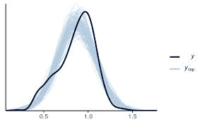
checking for non-normal error terms (Assumption A3 in Section 2.10).
One problem is that the tests are not great. The tests will indicate whether there is statisticallysignificant evidence for heteroskedasticity or non-normal error terms, but they certainly cannot prove that there is not any heteroskedasticity or non-normal error terms.

Regarding heteroskedasticity, your regression probably has heteroskedasticity. And, given that it is costless and painless to fix, you should probably include the heteroskedasticity correction.

Regarding non-normal error terms, recall that, due to the Central Limit Theorem, error terms will be approximately normal if the sample size is large enough (i.e., at least 200 observations at worst, and perhaps only 15 observations would suffice). However, this is not necessarily the case if: (1) the dependent variable is a dummy variable; and (2) there is not a large-enough set of explanatory variables. That said, a problem is that the test for non-normality (which tests for skewness and kurtosis) is highly unstable for small samples.

Having non-normal error terms means that the t-distribution would not apply to the standard errors, so the $t$-stats, standard levels of significance, confidence intervals, and $\mathrm{p}$-values would be a little off-target. The simple solution for cases in which there is the potential for non-normal errors is to require a lower $\mathrm{p}$-value than you otherwise would to conclude that there is a relationship between the explanatory and dependent variables.

I am not overly concerned by problems with non-normal errors because they are small potatoes when weighed against the Bayes critique of $\mathrm{p}$-values and the potential biases from PITFALLS (Chapter 6). If you have a valid study that is pretty convincing in terms of the PITFALLS being unlikely and having low-enough p-values in light of the Bayes critique, then having non-normal error terms would most likely not matter.

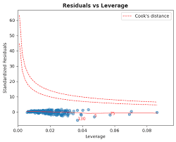
One potentially-useful diagnostic would be to check for outliers having large effects on the coefficient estimates. This would likely not be a concern with dependent variables that have a compact range of possible values, such as academic achievement test scores. But it could be the case with dependent variables on individual/family income or corporate profits/revenue, among other such outcomes with potentially large-outlying values of the dependent variable. Extreme values of explanatory variables could also be problematic. In these situations, it could be worth a diagnostic check of outliers for the dependent variable or the residuals. One could estimate the model without the big outliers to see how the results are affected. Of course, the outliers are supposedly legitimate observations, so any results without the outliers are not necessarily more correct. The ideal situation would be that the direction and magnitude of the estimates are consistent between the models with and without the outliers.
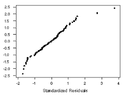
Outliers, if based on residuals, could be detected by residual plots. Alternatively, one potential rule that could be used for deleting outliers is based on calculating the standardized residual, which is the actual residual divided by the standard deviation of the residual-there is no need to subtract the mean of the residual since it is zero. The standardized residual indicates how many standard deviations away from zero a residual is. One could use an outlier rule, such as deleting observations with the absolute value of the standardized residual greater than some value, say, 5. With the adjusted sample, one would re-estimate a model to determine how stable the main results are.

统计代写|线性回归分析代写linear regression analysis代考|What the research on the hot hand in basketball tells us about

A friend of mine, drawn to the larger questions on life, called me recently and said that we are all alone – that humans are the only intelligent life in the universe. Rather than questioning him on the issue I have struggled with (whether humans, such as myself, should be categorized as “intelligent” life), I decided to focus on the main issue he raised and asked how he came to such a conclusion. Apparently, he had installed one of those contraptions in his backyard that searches for aliens. Honestly, he has so much junk in his backyard that I hadn’t even noticed. He said that he hadn’t received any signals in two years, so we must be alone.

While I have no idea whether we are alone in the universe, I know that my curious friend is not alone in his logic. A recent Wall Street Journal article made a similar logical conclusion in an article with some plausible arguments on why humans may indeed be alone in the universe. One of those arguments was based on the “deafening silence” from the 40-plus-year Search for Extraterrestrial Intelligence (SETI) project, with the conclusion that this is strong evidence that there is no other intelligent life (Metaxas, 2014). Never mind that SETI only searches our galaxy (of the estimated 170-plus billion galaxies in the universe) and that for us to find life on some planet, we have to be aiming our SETI at that planet (instead of the other 100 billion or so planets in our galaxy) at the same time (within the 13.6 billion years our galaxy has been in existence) that the alien geeks on that planet are emitting strong-enough radio signals in our direction (with a 600-plus-year lag for the radio signals to reach us). It may be that some form of aliens sent radio signals our way 2.8 billion years ago (before they went extinct after elininating their Environmental Protection Ageney), purposefully-striked-through and our amoeba-like ancestors had not yet developed the SETI technology to detect the signals.

The flawed logic here, as you have probably determined, is that lack of evidence is not proof of non-existence. This is particularly the case when you have a weak test for what you are looking for.
This logic flaw happens to be very common among academics. One line of research that has been subject to such faulty logic is that on the hot hand in basketball. The “hot hand” is a situation in which a player has a period (often within a single game) with a systematically higher probability of making shots (adjusting for the difficulty of the shot) than the player normally would have. The hot hand can occur in just about any other sport or activity, such as baseball, bowling, dance, test-taking, etc. In basketball, virtually all players and fans believe in the hot hand, based on witnessing players such as Stephen Curry go through stretches in which they make a series of high-difficulty shots. Yet, from 1985 to 2009 , plenty of researchers tested for the hot hand in basketball by using various tests to essentially determine whether a player was more likely to make a shot after a made shot (or consecutive made shots) than after a missed shot. They found no evidence of the hot hand. Their conclusion was “the hot hand is a myth.”
But then a few articles, starting in 2010, found evidence for the hot hand. And, as Stone (2012), Arkes (2013), and Miller and Sanjurjo (2018) show, the tests for the studies in the first 25 years were pretty weak tests for the hot hand because of some modeling problems, one of which I will describe in Box 6.4 in the next chapter.

The conclusions from those pre-2010 studies should not have been “the hot hand is a myth,” but rather “there is no evidence for the hot hand in basketball.” The lack of evidence was not proof of the non-existence of the hot hand. Using the same logic, in the search for aliens, the lack of evidence is not proof of non-existence, especially given that the tests have been weak. ${ }^5 \mathrm{I}$ ‘d bet my friend’s SETI machine that the other life forms out there, if they exist, would make proper conclusions on the basketball hot hand (and that they won’t contact us until we collectively get it right on the hot hand).

线性回归代写

统计代写|线性回归分析代写linear regression analysis代考|What model diagnostics should you do?

没有任何！好吧，大多数时候，没有。这是我的观点，我可能是错的。其他人（包括你的教授）可能有正当理由不同意。但这是为什么在大多数情况下不需要执行任何模型诊断的论点。
进行的两种最常见的模型诊断是：

检查异方差
检查非正态误差项（第 2.10 节中的假设 A3）。
一个问题是测试不是很好。检验将表明是否存在异方差或非正态误差项的统计显着证据，但它们当然不能证明不存在任何异方差或非正态误差项。

关于异方差性，您的回归可能具有异方差性。而且，鉴于修复起来既无成本又无痛，您可能应该包括异方差校正。

关于非正态误差项，回想一下，根据中心极限定理，如果样本量足够大（即最坏情况下至少有 200 个观测值，也许只有 15 个观测值就足够了），误差项将近似为正态。但是，如果出现以下情况则不一定如此： (1) 因变量是虚拟变量；(2) 没有足够大的解释变量集。也就是说，一个问题是非正态性测试（测试偏度和峰度）对于小样本来说非常不稳定。

具有非正态误差项意味着 t 分布不适用于标准误差，因此吨-统计、显着性标准水平、置信区间和p-values 会有点偏离目标。对于可能出现非正态错误的情况，简单的解决方案是要求较低的p-value 比你否则得出的结论是解释变量和因变量之间存在关系。

我并不过分担心非正态误差的问题，因为当与贝叶斯对p-来自 PITFALLS（第 6 章）的价值观和潜在偏见。如果您有一项有效的研究，就 PITFALLS 不太可能并且根据贝叶斯批判具有足够低的 p 值而言，该研究非常有说服力，那么具有非正态误差项很可能无关紧要。

一种可能有用的诊断方法是检查对系数估计值有很大影响的异常值。对于具有紧凑可能值范围的因变量（例如学业成绩测试分数），这可能不是一个问题。但是，个人/家庭收入或公司利润/收入的因变量可能就是这种情况，以及其他具有因变量的潜在大异常值的结果。解释变量的极值也可能有问题。在这些情况下，可能值得对因变量或残差的异常值进行诊断检查。人们可以在没有大异常值的情况下估计模型，看看结果是如何受到影响的。当然，离群值应该是合法的观察结果，所以没有异常值的任何结果都不一定更正确。理想情况是估计的方向和大小在有和没有异常值的模型之间是一致的。
如果基于残差，则可以通过残差图检测异常值。或者，可用于删除离群值的一个潜在规则是基于计算标准化残差，即实际残差除以残差的标准差——无需减去残差的均值，因为它为零。标准化残差表示残差与零的标准差有多少。可以使用异常值规则，例如删除标准化残差的绝对值大于某个值（例如 5）的观测值。使用调整后的样本，可以重新估计模型以确定主要结果的稳定性。

统计代写|线性回归分析代写linear regression analysis代考|What the research on the hot hand in basketball tells us about

我的一个朋友被生命中更大的问题所吸引，最近给我打电话说我们都是孤独的——人类是宇宙中唯一的智慧生命。我没有就我一直在纠结的问题（人类，比如我自己，是否应该被归类为“智能”生命）质疑他，而是决定专注于他提出的主要问题，并询问他是如何得出这样的结论的。显然，他在自家后院安装了其中一个搜索外星人的装置。老实说，他的后院有那么多垃圾，我什至都没注意到。他说他已经两年没有收到任何信号了，所以我们肯定是一个人。

虽然我不知道我们在宇宙中是否是孤独的，但我知道我好奇的朋友在他的逻辑上并不孤单。《华尔街日报》最近的一篇文章在一篇文章中得出了类似的逻辑结论，并就为什么人类在宇宙中确实可能是孤独的提出了一些似是而非的论据。其中一个论点是基于 40 多年的搜寻外星智能 (SETI) 项目的“震耳欲聋的沉默”，得出的结论是，这是不存在其他智慧生命的有力证据（Metaxas，2014 年）。不要介意 SETI 只搜索我们的星系（宇宙中估计有 170 多亿个星系），为了让我们在某个星球上找到生命，我们必须将 SETI 瞄准那个星球（而不是其他 1000 亿或所以我们银河系中的行星）同时（在 13. 我们的银河系已经存在了 60 亿年），那个星球上的外星极客正在向我们的方向发射足够强的无线电信号（无线电信号到达我们有 600 多年的滞后）。可能是某种形式的外星人在 28 亿年前（在他们取消环境保护署后灭绝之前）向我们发送了无线电信号，有目的地通过，而我们的变形虫类祖先尚未开发出 SETI 技术来检测信号。

正如您可能已经确定的那样，这里有缺陷的逻辑是缺乏证据并不能证明不存在。当您对要查找的内容进行弱测试时尤其如此。
这种逻辑缺陷恰好在学术界非常普遍。受制于这种错误逻辑的一项研究是关于篮球的热手。“热手”是这样一种情况，在这种情况下，一名球员有一段时间（通常在一场比赛中）比球员通常有更高的投篮概率（根据投篮难度进行调整）。热手几乎可以发生在任何其他运动或活动中，例如棒球、保龄球、舞蹈、应试等。在篮球运动中，几乎所有球员和球迷都相信热手，这是基于斯蒂芬库里等球员的见证经历他们进行一系列高难度投篮的阶段。然而，从 1985 年到 2009 年，许多研究人员通过各种测试来测试篮球中的热手，从根本上确定一名球员在投篮命中（或连续投篮命中）后是否比投丢后更有可能投篮。他们没有发现热手的证据。他们的结论是“热手是一个神话”。
但是从 2010 年开始的几篇文章找到了热手的证据。而且，正如 Stone（2012 年）、Arkes（2013 年）以及 Miller 和 Sanjurjo（2018 年）所表明的那样，由于某些建模问题，前 25 年的研究测试对热手的测试非常薄弱，其中之一是我将在下一章专栏 6.4 中描述。

那些 2010 年之前的研究得出的结论不应该是“热手是一个神话”，而是“篮球中没有热手的证据”。缺乏证据并不能证明热手不存在。使用相同的逻辑，在寻找外星人时，缺乏证据并不是不存在的证据，特别是考虑到测试一直很薄弱。5我我敢打赌我朋友的 SETI 机器，如果存在其他生命形式，他们会在篮球热手上做出正确的结论（并且他们不会联系我们，直到我们共同在热手上找到它）。

统计代写|线性回归分析代写linear regression analysis代考请认准statistics-lab™

统计代写请认准statistics-lab™. statistics-lab™为您的留学生涯保驾护航。

随机过程代考

在概率论概念中，随机过程是随机变量的集合。若一随机系统的样本点是随机函数，则称此函数为样本函数，这一随机系统全部样本函数的集合是一个随机过程。实际应用中，样本函数的一般定义在时间域或者空间域。 随机过程的实例如股票和汇率的波动、语音信号、视频信号、体温的变化，随机运动如布朗运动、随机徘徊等等。

贝叶斯方法代考

贝叶斯统计概念及数据分析表示使用概率陈述回答有关未知参数的研究问题以及统计范式。后验分布包括关于参数的先验分布，和基于观测数据提供关于参数的信息似然模型。根据选择的先验分布和似然模型，后验分布可以解析或近似，例如，马尔科夫链蒙特卡罗 (MCMC) 方法之一。贝叶斯统计概念及数据分析使用后验分布来形成模型参数的各种摘要，包括点估计，如后验平均值、中位数、百分位数和称为可信区间的区间估计。此外，所有关于模型参数的统计检验都可以表示为基于估计后验分布的概率报表。

广义线性模型代考

广义线性模型（GLM）归属统计学领域，是一种应用灵活的线性回归模型。该模型允许因变量的偏差分布有除了正态分布之外的其它分布。

statistics-lab作为专业的留学生服务机构，多年来已为美国、英国、加拿大、澳洲等留学热门地的学生提供专业的学术服务，包括但不限于Essay代写，Assignment代写，Dissertation代写，Report代写，小组作业代写，Proposal代写，Paper代写，Presentation代写，计算机作业代写，论文修改和润色，网课代做，exam代考等等。写作范围涵盖高中，本科，研究生等海外留学全阶段，辐射金融，经济学，会计学，审计学，管理学等全球99%专业科目。写作团队既有专业英语母语作者，也有海外名校硕博留学生，每位写作老师都拥有过硬的语言能力，专业的学科背景和学术写作经验。我们承诺100%原创，100%专业，100%准时，100%满意。

机器学习代写

随着AI的大潮到来，Machine Learning逐渐成为一个新的学习热点。同时与传统CS相比，Machine Learning在其他领域也有着广泛的应用，因此这门学科成为不仅折磨CS专业同学的“小恶魔”，也是折磨生物、化学、统计等其他学科留学生的“大魔王”。学习Machine learning的一大绊脚石在于使用语言众多，跨学科范围广，所以学习起来尤其困难。但是不管你在学习Machine Learning时遇到任何难题，StudyGate专业导师团队都能为你轻松解决。

多元统计分析代考

基础数据: $N$ 个样本， $P$ 个变量数的单样本，组成的横列的数据表
变量定性: 分类和顺序；变量定量：数值
数学公式的角度分为: 因变量与自变量

时间序列分析代写

随机过程，是依赖于参数的一组随机变量的全体，参数通常是时间。随机变量是随机现象的数量表现，其时间序列是一组按照时间发生先后顺序进行排列的数据点序列。通常一组时间序列的时间间隔为一恒定值（如1秒，5分钟，12小时，7天，1年），因此时间序列可以作为离散时间数据进行分析处理。研究时间序列数据的意义在于现实中，往往需要研究某个事物其随时间发展变化的规律。这就需要通过研究该事物过去发展的历史记录，以得到其自身发展的规律。

回归分析代写

多元回归分析渐进（Multiple Regression Analysis Asymptotics）属于计量经济学领域，主要是一种数学上的统计分析方法，可以分析复杂情况下各影响因素的数学关系，在自然科学、社会和经济学等多个领域内应用广泛。

MATLAB代写

MATLAB 是一种用于技术计算的高性能语言。它将计算、可视化和编程集成在一个易于使用的环境中，其中问题和解决方案以熟悉的数学符号表示。典型用途包括：数学和计算算法开发建模、仿真和原型制作数据分析、探索和可视化科学和工程图形应用程序开发，包括图形用户界面构建MATLAB 是一个交互式系统，其基本数据元素是一个不需要维度的数组。这使您可以解决许多技术计算问题，尤其是那些具有矩阵和向量公式的问题，而只需用 C 或 Fortran 等标量非交互式语言编写程序所需的时间的一小部分。MATLAB 名称代表矩阵实验室。MATLAB 最初的编写目的是提供对由 LINPACK 和 EISPACK 项目开发的矩阵软件的轻松访问，这两个项目共同代表了矩阵计算软件的最新技术。MATLAB 经过多年的发展，得到了许多用户的投入。在大学环境中，它是数学、工程和科学入门和高级课程的标准教学工具。在工业领域，MATLAB 是高效研究、开发和分析的首选工具。MATLAB 具有一系列称为工具箱的特定于应用程序的解决方案。对于大多数 MATLAB 用户来说非常重要，工具箱允许您学习和应用专业技术。工具箱是 MATLAB 函数（M 文件）的综合集合，可扩展 MATLAB 环境以解决特定类别的问题。可用工具箱的领域包括信号处理、控制系统、神经网络、模糊逻辑、小波、仿真等。

R语言代写	问卷设计与分析代写
PYTHON代写	回归分析与线性模型代写
MATLAB代写	方差分析与试验设计代写
STATA代写	机器学习/统计学习代写
SPSS代写	计量经济学代写
EVIEWS代写	时间序列分析代写
EXCEL代写	深度学习代写
SQL代写	各种数据建模与可视化代写

统计代写|线性回归分析代写linear regression analysis代考|Consequences of measurement error

Posted on 2023年4月28日2023年4月28日 by statistics-lab

如果你也在怎样代写线性回归分析linear regression analysis这个学科遇到相关的难题，请随时右上角联系我们的24/7代写客服。

我们提供的线性回归分析linear regression analysis及其相关学科的代写，服务范围广, 其中包括但不限于:

Statistical Inference 统计推断
Statistical Computing 统计计算
Advanced Probability Theory 高等楖率论
Advanced Mathematical Statistics 高等数理统计学
(Generalized) Linear Models 广义线性模型
Statistical Machine Learning 统计机器学习
Longitudinal Data Analysis 纵向数据分析
Foundations of Data Science 数据科学基础

统计代写|线性回归分析代写linear regression analysis代考|Consequences of measurement error

Suppose that the average income for those without and with a college degree is as depicted in Figure 6.8. On average, those with a college degree earn $\$ 40,000$ more than those without a college degree.
Now suppose that a random sample of people with a college degree were misassigned to the no-college-degree group. Assuming that this sample of the misassigned were fairly representative of the college-degree group, this would raise the average income for the no-college-degree group. This would then reduce the difference in average income between the two groups. Conversely, let’s say that part of the no-college-degree group is misassigned to the college-degree group. This would likely lower the average income of the college-degree group, again reducing the difference. The measurement error would cause the observed difference in incomes between the two groups to be lower than the actual differences.

This demonstrates the effects of an explanatory variable being measured with error. It typically causes the coefficient estimate to be biased towards zero, which is called attenuation bias. If the explanatory variable were a variable with many possible values (such as years-of-schooling) rather than just a dummy variable, the same concept applies: the misclassification from measurement error would typically cause a bias towards zero in the coefficient estimate on the variable.

Let’s use some actual data to test for the effects of measurement error. In Table 6.6, I show the results of two models:

Column (1) is the same as the Multiple Regression model from Table 5.1 in Section 5.1, except that a dummy variable for having a “college degree” is used instead of “years-of-schooling” and the standard errors are now corrected for heteroskedasticity
Column (2) is the same except that I switched the “college degree” assignment for a randomly-selected part of the sample. That is, for about $10 \%$ of the sample (those who had a randomly-generated variable in the $[0,1]$ range be $<0.1)$, I set the college-degree variable equal to 1 if it was originally 0 and vice versa.

What we see is that the coefficient estimate on “college degree” is reduced significantly: from $\$ 28,739$ to $\$ 15,189$. Thus, the measurement error in the college-degree variable is causing a bias in the coefficient estimate towards zero. (Note that if you try to replicate this with the code on the book’s website, you will obtain different numbers due to the randomization, but the general story should be the same.)

统计代写|线性回归分析代写linear regression analysis代考|An example of including mediating factors as control variables

Let’s consider a case that comes from one of my publications (Arkes, 2007). In that study, I examined what happens to teenage drug use when the state unemployment rate increases, similar to the basic regression from Section 3.3. From the more-recent NLSY (starting in 1997), I had individual-level data of teenagers from all states and over several years. I specified the model as follows:
$$
Y_{i s t}=X_{i s t} \beta_1+\beta_2 U R_{s t}+\varepsilon_{\text {ist }}
$$
where $Y$ is the measure of teenage drug use, $U R$ is the state unemployment rate for state $s$ in year $t$. The vector $X$ would include a set of demographic variables, year dummy variables, and state dummy variables. This is nearly equivalent to using state and year fixed effects, which will be covered in Section 8.1. The $i$ subscript indicates that individual-level data is used.

When writing this article, I conceived of several mechanisms for how a higher unemployment rate could lead to a change in teenage drug use. They are represented in the top chart in Figure 6.9, which is similar in nature to Figures $4.7 \mathrm{a}$ and $4.7 \mathrm{~b}$. The first set of arrows on the left represents how an increase in the unemployment rate (by one percentage point) would affect three mediating factors.
Recall from Chapter 4 that mediating factors (also called “intervening factors” or “mechanism variables”) are factors through which the key-explanatory variable affects the dependent variable. For example, in the lemon-tree example, the tree’s height was a mediating factor for how watering affected the number of lemons the tree produced.

The second set of arrows represents how one-unit increases in those mediating factors would affect teenage drug use. Decreases in the mediating factors would cause the opposite effect. A mechanism would be a full reason why a change in the unemployment rate caused a change in teenage drug use, represented in Figure 6.9 as a full pathway, or one set of the left and right arrows. There are three mechanisms, labeled with circled M1, M2, and M3. Properly estimating the values of these mechanisms would be impossible because two of the mediating factors are unobservable and non-quantifiable, and there would be numerous biases in estimating how teenage income affected teen drug use. Furthermore, there could be a correlation between the various mechanisms, so the sum of the three mechanisms, if this were the complete set of mechanisms, would not necessarily be the true causal effect. Nevertheless, all of the mechanisms contribute to the overall effect of the unemployment rate on teen drug use, along with other mechanisms I might have missed.

线性回归代写

统计代写|线性回归分析代写linear regression analysis代考|Consequences of measurement error

假设没有和拥有大学学位的人的平均收入如图 6.8 所示。平均而言，拥有大学学位的人收入$40,000比没有大学学历的人多。
现在假设随机抽样的具有大学学位的人被错误地分配到没有大学学位的组中。假设这个被错误分配的样本在大学学历组中具有相当的代表性，这将提高没有大学学历组的平均收入。这将缩小两组之间平均收入的差异。相反，假设没有大学学位组的一部分被错误分配到大学学位组。这可能会降低大学学历人群的平均收入，再次缩小差距。测量误差会导致观察到的两组收入差异低于实际差异。

这证明了用误差测量的解释变量的影响。它通常会导致系数估计值偏向于零，这称为衰减偏差。如果解释变量是一个具有许多可能值的变量（例如受教育年限）而不仅仅是一个虚拟变量，则适用相同的概念：测量误差造成的错误分类通常会导致系数估计值偏向零多变的。

让我们使用一些实际数据来测试测量误差的影响。在表 6.6 中，我展示了两个模型的结果：

第 (1) 列与第 5.1 节表 5.1 中的多元回归模型相同，不同之处在于使用“大学学位”虚拟变量而不是“受教育年限”，标准误差现在已针对异方差性
第 (2) 列是相同的，只是我为随机选择的样本部分切换了“大学学位”分配。也就是说，对于大约10%的样本（那些在[0,1]范围是<0.1)，我将 college-degree 变量设置为等于 1，如果它最初是 0，反之亦然。

我们看到的是“大学学位”的系数估计值显着降低：来自$28,739到$15,189. 因此，大学学位变量的测量误差导致系数估计偏向于零。（请注意，如果您尝试使用本书网站上的代码复制它，由于随机化，您将获得不同的数字，但总体情况应该是相同的。）

统计代写|线性回归分析代写linear regression analysis代考|An example of including mediating factors as control variables

让我们考虑一个来自我的出版物 (Arkes，2007) 的案例。在那项研究中，我研究了当州失业率上升时青少年吸毒会发生什么情况，类似于第 3.3 节中的基本回归。从最近的 NLSY (从 1997 年开始)，我获得了来自所有州的青少年的个人水平数据，这些数据持续了数年。我指定的模型如下:
$$
Y_{i s t}=X_{i s t} \beta_1+\beta_2 U R_{s t}+\varepsilon_{\text {ist }}
$$
在哪里 $Y$ 是青少年吸毒的衡量标准， $U R$ 是州的州失业率 $s$ 在一年 $t$. 载体 $X$ 将包括一组人口统计变量、年份虚拟变量和州虚拟变量。这几乎等同于使用州和年份固定效应，这将在第 8.1 节中介绍。这 $i$ 下标表示使用个体水平的数据。
在撰写本文时，我设想了几种机制来解释较高的失业率如何导致青少年吸毒情况发生变化。它们在图 6.9 的顶部图表中表示，这在本质上类似于图4.7a和 $4.7 \mathrm{~b}$. 左边的第一组箭头表示失业率增加 (一个百分点）将如何影响三个中介因素。
回顾第 4 章，中介因素（也称为“干预因素”或“机制变量”）是关键解释变量影响因变量的因素。例如，在柠檬树的例子中，树的高度是浇水如何影响树产生的柠檬数量的中介因素。
第二组箭头表示这些中介因素增加一个单位将如何影响青少年吸毒。中介因素的减少会导致相反的效果。机制将是失业率变化导致青少年吸毒变化的完整原因，在图 6.9 中表示为完整路径，或一组左右箭头。共有三种机制，标有带圆圈的 M1、M2 和 M3。正确估计这些机制的价值是不可能的，因为其中两个中介因素是不可观察和不可量化的，而且在估计青少年收入如何影响青少年吸毒时会存在许多偏差。此外，各种机制之间可能存在相关性，因此三种机制的总和，如果这是一套完整的机制，不一定是真正的因果关系。尽管如此，所有这些机制都有助于失业率对青少年吸毒的总体影响，以及我可能错过的其他机制。

统计代写请认准statistics-lab™. statistics-lab™为您的留学生涯保驾护航。

随机过程代考

贝叶斯方法代考

广义线性模型代考

广义线性模型（GLM）归属统计学领域，是一种应用灵活的线性回归模型。该模型允许因变量的偏差分布有除了正态分布之外的其它分布。

机器学习代写

多元统计分析代考

基础数据: $N$ 个样本， $P$ 个变量数的单样本，组成的横列的数据表
变量定性: 分类和顺序；变量定量：数值
数学公式的角度分为: 因变量与自变量

时间序列分析代写

回归分析代写

MATLAB代写

R语言代写	问卷设计与分析代写
PYTHON代写	回归分析与线性模型代写
MATLAB代写	方差分析与试验设计代写
STATA代写	机器学习/统计学习代写
SPSS代写	计量经济学代写
EVIEWS代写	时间序列分析代写
EXCEL代写	深度学习代写
SQL代写	各种数据建模与可视化代写

统计代写|线性回归分析代写linear regression analysis代考|An example with a wider range of effects

Posted on 2023年4月28日2023年4月28日 by statistics-lab

如果你也在怎样代写线性回归分析linear regression analysis这个学科遇到相关的难题，请随时右上角联系我们的24/7代写客服。

我们提供的线性回归分析linear regression analysis及其相关学科的代写，服务范围广, 其中包括但不限于:

Statistical Inference 统计推断
Statistical Computing 统计计算
Advanced Probability Theory 高等楖率论
Advanced Mathematical Statistics 高等数理统计学
(Generalized) Linear Models 广义线性模型
Statistical Machine Learning 统计机器学习
Longitudinal Data Analysis 纵向数据分析
Foundations of Data Science 数据科学基础

统计代写|线性回归分析代写linear regression analysis代考|An example with a wider range of effects

Consider another example of the optimal assignment of military recruiters. Military personnel assigned as recruiters can typically request their duty locations, and many often request locations near their family or where they grew up. A service, say the Army, may be interested in estimating how assigning recruiters to their home county, on average, affects their productivity as a recruiter, or the number of contracts they get. The Army may estimate the following model:
$$
C_i=X_i \beta_1+\beta_2 H_i+\varepsilon_i
$$
where

$C=#$ contracts (or recruits) for a given recruiter in a given time period
$X=$ a set of characteristics of the recruiter and the location
$H=$ an indicator for being assigned to one’s home county.
The effect of recruiting in one’s home county would not be the same for all recruiters. Being back at home may positively affect productivity if the recruiter has old contacts or if the recruiter would be more trustworthy to potential recruits, being from the neighborhood, than other recruiters would be. On the other hand, for some people, being back home could negatively affect productivity because the recruiter spends more time with family and his/her homies.

Self-selection bias would apply if those who would be more successful at recruiting back home (relative to other areas) were more likely to be assigned to their home county (likely by requesting to do so). In contrast, the ideal situation for the researcher would be that recruiters are assigned to their home county regardless of their individual causal effect.

As a visual depiction, consider the sample of seven recruiters in Figure 6.7, which shows in the top chart the frequency distribution of the true effect for a sample of seven recruiters. So the effect of home-county $(H)$ on the number of monthly contracts varies from -0.3 to 0.3 in 0.1 increments, with each recruiter having their own effect. The Average Treatment Effect is 0.0 , which is the average of the seven individual effects. This would be the average impact on recruiting if all seven were assigned to their home county.

In the bottom chart, I show a likely situation in which only some of the recruiters are assigned to their home county, marked by the bars being filled in for the four recruiters assigned to their home county $(H=1)$ and the bars being unfilled for the other three $(H=0)$. I purposefully made it so it is not just those with the higher effects who are assigned to their home state, as recruiters might not correctly predict how successful they would be back home, and other factors, such as the Army’s needs, could determine where a recruiter would be assigned.

What the researcher observes is the impact just for those who receive the treatment. For completeness of the example, let me assume that the recruiters would be equally successful if all were not assigned to their home county. The average effect we would observe would be $(-0.1+0+0.2+$ $0.3) \div 4=0.1$. This overstates the true average effect of 0.0 . Thus, there is a positive bias from the tendency of recruiters to request their home county if they think they’d be successful there.

统计代写|线性回归分析代写linear regression analysis代考|An example of the effects of minimum-wage increases

At the time I write this, there has not been a U.S. federal minimum-wage increase in 13 years, as it currently stands at $\$ 7.20$. There have been discussions to raise it to $\$ 15$, but there is great opposition to that proposal. At the same time, some high-cost cities have already raised the minimum wage to around that figure (e.g., $\$ 14.49$ in Seattle and $\$ 16.32$ in San Francisco).

There have been hundreds of studies examining how minimum-wage increases affect employment levels. The results have been all over the map, with some studies finding negative impacts and other studies finding positive impacts, but they tend towards minimum-wage increases leading to reduced employment.
This is a classic case of there not being a single effect for all subjects (in this case, the subject is a city or state). For example, if the federal minimum wage were increased to $\$ 15$, there would be minimalto-no impact in Seattle, San Francisco, and many other high-cost cities and states in which wages are already fairly high. In contrast, in low-cost areas (e.g., Mississippi), there is the potential for greater negative effects on employment.

Most minimum-wage studies rely on data on state-level (or city-level) minimum-wage changes. However, because of these varying effects, there is great potential for self-selection bias in such studies. It is not random as to which cities or states enact minimum-wage increases, as they would tend to be the ones that would be able to more easily absorb the minimum-wage increase. Perhaps average wages for low-skill workers are already high, or maybe a city has such strong economic growth that people would pay higher prices for their coffee or other products that would have greater costs with the minimum-wage increase.

This would mean that we would have self-selection bias in that we would be more likely to observe minimum-wage increases with less-harmful or less-negative effects than would be the average effect across the country. Again, this would bias the estimated effect in the more-beneficial direction, which would be less employment loss in this case.

线性回归代写

统计代写|线性回归分析代写linear regression analysis代考|An example with a wider range of effects

考虑另一个军事招募人员最佳分配的例子。被指派为招聘人员的军事人员通常可以请求他们的工作地点，许多人经常请求靠近他们家人或他们长大的地方。陆军说，某项服务可能有兴趣估计平均而言，将招聘人员分配到他们所在的县对他们作为招聘人员的生产力或他们获得的合同数量有何影响。陆军可能会估计以下模型:
$$
C_i=X_i \beta_1+\beta_2 H_i+\varepsilon_i
$$
在哪里

$C=#$ 给定时间段内给定招聘人员的合同（或招聘)
$X=$ 招聘人员的一组特征和位置
$H=$ 被分配到一个人的家乡的指标。
在家乡招聘的效果对所有招聘人员来说都是不一样的。如果招聘人员有老联系人，或者如果招聘人员来自附近，比其他招聘人员更值得潜在招聘人员信任，那么回到家里可能会对工作效率产生积极影响。另一方面，对于某些人来说，回家可能会对工作效率产生负面影响，因为招聘人员会花更多的时间与家人和他/她的朋友在一起。
如果那些在家乡 (相对于其他地区) 招募更成功的人更有可能被分配到他们的家乡 (可能通过要求伩样做），那么自我选择偏差就会适用。相比之下，研究人员的理想情况是招聘人员被分配到他们的家乡，而不考虑他们的个人因果效应。
作为可视化描述，请考虑图 6.7 中七名招聘人员的样本，该图在顶部图表中显示了七名招聘人员样本的真实效果的频率分布。所以家乡的效果 $(H)$ 每月合同的数量从 -0.3 到 0.3 不等，增量为 0.1 ，每个招聘人员都有自己的影响。平均处理效果为 0.0 ，这是七个单独效果的平均值。如果所有七人都被分配到他们的家乡，这将是对招聘的平均影响。
在底部的图表中，我展示了一种可能的情况，其中只有一些招聘人员被分配到他们所在的县，由分配到他们所在县的四名招聘人员填充的条形标记 $(H=1)$ 并且其他三个末填充的条形图 $(H=0)$. 我是故意这样做的，这样不仅那些影响力较高的人会被分配到他们的家乡，因为招聘人员可能无法正确预测他们在家乡的成功程度，而其他因素 (例如军队的需求) 可以确定他们在哪里将分配招聘人员。
研究人员观察到的只是对接受治疗的人的影响。为了示例的完整性，让我假设如果不是所有人都被分配到他们的家乡，招聘人员也会同样成功。我们观察到的平均效果是 $(-0.1+0+0.2+0.3) \div 4=0.1$. 这夸大 30.0 的真实平均效果。因此，如果招聘人员认为他们会在家乡取得成功，他们倾向于要求他们所在的县，这是一种积极的偏见。

统计代写|线性回归分析代写linear regression analysis代考|An example of the effects of minimum-wage increases

在我写这篇文章的时候，美国联邦最低工资已经 13 年没有增加了，目前是$7.20. 已经有人讨论将其提高到$15，但该提议遭到强烈反对。与此同时，一些高成本城市已经将最低工资提高到这个数字附近（例如，$14.49在西雅图和$16.32在旧金山）。

已有数百项研究探讨最低工资增长如何影响就业水平。结果无处不在，一些研究发现了负面影响，而另一些研究则发现了积极影响，但它们倾向于提高最低工资，从而导致就业减少。
这是一个经典案例，没有对所有主题（在这种情况下，主题是城市或州）产生单一影响。例如，如果联邦最低工资提高到$15，对西雅图、旧金山和许多其他工资已经相当高的高成本城市和州，影响很小甚至没有。相比之下，在低成本地区（例如密西西比州），可能会对就业产生更大的负面影响。

大多数最低工资研究依赖于州级（或城市级）最低工资变化的数据。然而，由于这些不同的影响，在此类研究中存在很大的自我选择偏差的可能性。哪些城市或州实施最低工资增长并不是随机的，因为它们往往是能够更容易吸收最低工资增长的城市或州。也许低技能工人的平均工资已经很高，或者也许一个城市的经济增长如此强劲，以至于人们会为他们的咖啡或其他产品支付更高的价格，而最低工资的增加会增加成本。

这意味着我们会有自我选择偏差，因为我们更有可能观察到最低工资的增加带来的危害或负面影响小于全国的平均影响。同样，这会使估计的影响偏向更有利的方向，在这种情况下，这将减少就业损失。

统计代写请认准statistics-lab™. statistics-lab™为您的留学生涯保驾护航。

随机过程代考

贝叶斯方法代考

广义线性模型代考

广义线性模型（GLM）归属统计学领域，是一种应用灵活的线性回归模型。该模型允许因变量的偏差分布有除了正态分布之外的其它分布。

机器学习代写

多元统计分析代考

基础数据: $N$ 个样本， $P$ 个变量数的单样本，组成的横列的数据表
变量定性: 分类和顺序；变量定量：数值
数学公式的角度分为: 因变量与自变量

时间序列分析代写

回归分析代写

MATLAB代写

R语言代写	问卷设计与分析代写
PYTHON代写	回归分析与线性模型代写
MATLAB代写	方差分析与试验设计代写
STATA代写	机器学习/统计学习代写
SPSS代写	计量经济学代写
EVIEWS代写	时间序列分析代写
EXCEL代写	深度学习代写
SQL代写	各种数据建模与可视化代写

统计代写|线性回归分析代写linear regression analysis代考|Plots for the Multivariate Linear Regression Model

Posted on 2023年4月26日2023年4月26日 by statistics-lab

如果你也在怎样代写线性回归分析linear regression analysis这个学科遇到相关的难题，请随时右上角联系我们的24/7代写客服。

我们提供的线性回归分析linear regression analysis及其相关学科的代写，服务范围广, 其中包括但不限于:

Statistical Inference 统计推断
Statistical Computing 统计计算
Advanced Probability Theory 高等楖率论
Advanced Mathematical Statistics 高等数理统计学
(Generalized) Linear Models 广义线性模型
Statistical Machine Learning 统计机器学习
Longitudinal Data Analysis 纵向数据分析
Foundations of Data Science 数据科学基础

统计代写|线性回归分析代写linear regression analysis代考|Plots for the Multivariate Linear Regression Model

This section suggests using residual plots, response plots, and the DD plot to examine the multivariate linear model. The residual plots are often used to check for lack of fit of the multivariate linear model. The response plots are used to check linearity and to detect influential cases and outliers. The response and residual plots are used exactly as in the $m=1$ case corresponding to multiple linear regression and experimental design models. See earlier chapters of this book, Olive et al. (2015), Olive and Hawkins (2005), and Cook and Weisberg (1999a, p. 432; 1999b).

Notation. Plots will be used to simplify the regression analysis, and in this text a plot of $W$ versus $Z$ uses $W$ on the horizontal axis and $Z$ on the vertical axis.

Definition 12.5. A response plot for the $j$ th response variable is a plot of the fitted values $\widehat{Y}{i j}$ versus the response $Y{i j}$. The identity line with slope one and zero intercept is added to the plot as a visual aid. A residual plot corresponding to the $j$ th response variable is a plot of $\hat{Y}{i j}$ versus $r{i j}$.

Remark 12.1. Make the $m$ response and residual plots for any multivariate linear regression. In a response plot, the vertical deviations from the identity line are the residuals $r_{i j}=Y_{i j}-\hat{Y}_{i j}$. Suppose the model is good, the $j$ th error distribution is unimodal and not highly skewed for $j=1, \ldots, m$, and $n \geq 10 p$. Then the plotted points should cluster about the identity line in each of the $m$ response plots. If outliers are present or if the plot is not linear, then the current model or data need to be transformed or corrected. If the model is good, then each of the $m$ residual plots should be ellipsoidal with no trend and should be centered about the $r=0$ line. There should not be any pattern in the residual plot: as a narrow vertical strip is moved from left to right, the behavior of the residuals within the strip should show little change. Outliers and patterns such as curvature or a fan shaped plot are bad.

统计代写|线性回归分析代写linear regression analysis代考|Asymptotically Optimal Prediction Regions

In this section, we will consider a more general multivariate regression model, and then consider the multivariate linear model as a special case. Given $n$ cases of training or past data $\left(\boldsymbol{x}_1, \boldsymbol{y}_1\right), \ldots,\left(\boldsymbol{x}_n, \boldsymbol{y}_n\right)$ and a vector of predictors $\boldsymbol{x}_f$, suppose it is desired to predict a future test vector $\boldsymbol{y}_f$.

Definition 12.8. A large sample $100(1-\delta) \%$ prediction region is a set $\mathcal{A}_n$ such that $P\left(\boldsymbol{y}_f \in \mathcal{A}_n\right) \rightarrow 1-\delta$ as $n \rightarrow \infty$, and is asymptotically optimal if the volume of the region converges in probability to the volume of the population minimum volume covering region.

The classical large sample $100(1-\delta) \%$ prediction region for a future value $\boldsymbol{x}f$ given iid data $\boldsymbol{x}_1, \ldots, \boldsymbol{x}_n$ is $\left{\boldsymbol{x}: D{\boldsymbol{x}}^2(\overline{\boldsymbol{x}}, \boldsymbol{S}) \leq \chi_{p, 1-\delta}^2\right}$, while for multivariate linear regression, the classical large sample $100(1-\delta) \%$ prediction region for a future value $\boldsymbol{y}f$ given $\boldsymbol{x}_f$ and past data $\left(\boldsymbol{x}_1, \boldsymbol{y}_i\right), \ldots,\left(\boldsymbol{x}_n, \boldsymbol{y}_n\right)$ is $\left{\boldsymbol{y}: D{\boldsymbol{y}}^2\left(\hat{\boldsymbol{y}}f, \hat{\boldsymbol{\Sigma}}{\boldsymbol{\epsilon}}\right) \leq \chi_{m, 1-\delta}^2\right}$. See Johnson and Wichern (1988, pp. 134, 151, $312)$. By equation $(10.10)$, these regions may work for multivariate normal $\boldsymbol{x}i$ or $\boldsymbol{\epsilon}_i$, but otherwise tend to have undercoverage. Olive (2013a) replaced $\chi{p, 1-\delta}^2$ by the order statistic $D_{\left(U_n\right)}^2$ where $U_n$ decreases to $\lceil n(1-\delta)\rceil$. This section will use a similar technique from Olive (2016b) to develop possibly the first practical large sample prediction region for the multivariate linear model with unknown error distribution. The following technical theorem will be needed to prove Theorem 12.4.

Theorem 12.3. Let $a>0$ and assume that $\left(\hat{\boldsymbol{\mu}}n, \hat{\boldsymbol{\Sigma}}_n\right)$ is a consistent estimator of $(\boldsymbol{\mu}, a \boldsymbol{\Sigma})$. a) $D{\boldsymbol{x}}^2\left(\hat{\boldsymbol{\mu}}n, \hat{\boldsymbol{\Sigma}}_n\right)-\frac{1}{a} D{\boldsymbol{x}}^2(\boldsymbol{\mu}, \boldsymbol{\Sigma})=o_P(1)$.
b) Let $0<\delta \leq 0.5$. If $\left(\hat{\boldsymbol{\mu}}n, \hat{\boldsymbol{\Sigma}}_n\right)-(\boldsymbol{\mu}, a \boldsymbol{\Sigma})=O_p\left(n^{-\delta}\right)$ and $a \hat{\boldsymbol{\Sigma}}_n^{-1}-\boldsymbol{\Sigma}^{-1}=$ $O_P\left(n^{-\delta}\right)$, then $$ D{\boldsymbol{x}}^2\left(\hat{\boldsymbol{\mu}}n, \hat{\boldsymbol{\Sigma}}_n\right)-\frac{1}{a} D{\boldsymbol{x}}^2(\boldsymbol{\mu}, \boldsymbol{\Sigma})=O_P\left(n^{-\delta}\right)
$$

线性回归代写

统计代写|线性回归分析代写linear regression analysis代考|Plots for the Multivariate Linear Regression Model

本节建议使用残差图、响应图和 DD 图来检查多元线性模型。残差图通常用于检查多元线性模型的拟合不足。响应图用于检查线性并检测有影响的个案和离群值。响应图和残差图的使用与 $m=1$ 对应于多元线性回归和实验设计模型的案例。请参阅本书的前几章，Olive 等人。(2015)、Olive 和 Hawkins (2005)，以及 Cook 和 Weisberg (1999a, p. 432; 1999b)。
符号。绘图将用于简化回归分析，在本文中的绘图 $W$ 相对 $Z$ 使用 $W$ 在水平轴上和 $Z$ 在垂直轴上。
定义 12.5。的响应图 $j$ 第一个响应变量是拟合值图 $\widehat{Y} i j$ 与响应 $Y i j$. 带有斜率 1 和零截距的标识线作为视觉辅助添加到图中。残差图对应于 $j$ 第一个响应变量是 $\hat{Y} i j$ 相对 $r i j$.
备注 12.1。让 $m$ 任何多元线性回归的响应和残差图。在响应图中，与标识线的垂直偏差是残差 $r_{i j}=Y_{i j}-\hat{Y}_{i j}$. 假设模型很好，则 $j$ th 错误分布是单峰的并且不是高度偏斜的 $j=1, \ldots, m$ ，和 $n \geq 10 p$. 然后绘制的点应该聚集在每个 $m$ 响应图。如果存在异常值或绘图不是线性的，则需要转换或校正当前模型或数据。如果模型很好，那么每个 $m$ 残差图应该是没有趋势的椭圆形，并且应该以 $r=0$ 线。残差图中不应该有任何模式：当一个宱的垂直条带从左向右移动时，条带内残差的行为应该显示出很小的变化。曲率或扇形图等异常值和模式是不好的。

统计代写|线性回归分析代写linear regression analysis代考|Asymptotically Optimal Prediction Regions

在本节中，我们将考虑更一般的多元回归模型，然后将多元线性模型视为特例。鉴于 $n$ 训练案例或过去的数据 $\left(\boldsymbol{x}1, \boldsymbol{y}_1\right), \ldots,\left(\boldsymbol{x}_n, \boldsymbol{y}_n\right)$ 和一个预测向量 $\boldsymbol{x}_f$ ，假设需要预测末来的测试向量 $\boldsymbol{y}_f$. 定义 12.8。大样本 $100(1-\delta) \%$ 预测区域是一个集合 $\mathcal{A}_n$ 这样 $P\left(\boldsymbol{y}_f \in \mathcal{A}_n\right) \rightarrow 1-\delta$ 作为 $n \rightarrow \infty$ ，并且如果该区域的体积在概率上收敛于人口最小体积覆盖区域的体积，则它是渐近最优的。经典大样本 $100(1-\delta) \%$ 末来值的预测区域 $\boldsymbol{x}$ 给定的 iid 数据 $\boldsymbol{x}_1, \ldots, \boldsymbol{x}_n$ 是，而对于多元线性回归，经典的大样本 $100(1-\delta) \%$ 末来值的预测区域 $\boldsymbol{y} f$ 给予 $\boldsymbol{x}_f$ 和过去的数据 $\left(\boldsymbol{x}_1, \boldsymbol{y}_i\right), \ldots,\left(\boldsymbol{x}_n, \boldsymbol{y}_n\right)$ 是 . 参见 Johnson 和 Wichern (1988 年，第 134、151 页，312). 通过等式 (10.10)，这些区域可能适用于多元正态 $\boldsymbol{x} i$ 或者 $\boldsymbol{\epsilon}_i$ ，但在其他方面往往有隐蔽性。橄榄 (2013a) 替换 $\chi p, 1-\delta^2$ 按顺序统计 $D{\left(U_n\right)}^2$ 在哪里 $U_n$ 减少到 $\lceil n(1-\delta)\rceil$. 本节将使用 Olive (2016b) 中的类似技术，为具有末知误差分布的多元线性模型开发可能是第一个实用的大样本预测区域。需要下面的技术定理来证明定理 12.4。
定理 12.3。让 $a>0$ 并假设 $\left(\hat{\boldsymbol{\mu}} n, \hat{\boldsymbol{\Sigma}}_n\right)$ 是一致的估计量 $(\boldsymbol{\mu}, a \boldsymbol{\Sigma})$. A)
$$
D \boldsymbol{x}^2\left(\hat{\boldsymbol{\mu}} n, \hat{\boldsymbol{\Sigma}}_n\right)-\frac{1}{a} D \boldsymbol{x}^2(\boldsymbol{\mu}, \boldsymbol{\Sigma})=o_P(1)
$$
b) 让 $0<\delta \leq 0.5$. 如果 $\left(\hat{\boldsymbol{\mu}} n, \hat{\mathbf{\Sigma}}_n\right)-(\boldsymbol{\mu}, a \boldsymbol{\Sigma})=O_p\left(n^{-\delta}\right)$ 和 $a \hat{\mathbf{\Sigma}}_n^{-1}-\boldsymbol{\Sigma}^{-1}=O_P\left(n^{-\delta}\right)$ ，然后
$$
D \boldsymbol{x}^2\left(\hat{\boldsymbol{\mu}} n, \hat{\boldsymbol{\Sigma}}_n\right)-\frac{1}{a} D \boldsymbol{x}^2(\boldsymbol{\mu}, \mathbf{\Sigma})=O_P\left(n^{-\delta}\right)
$$

统计代写请认准statistics-lab™. statistics-lab™为您的留学生涯保驾护航。

随机过程代考

贝叶斯方法代考

广义线性模型代考

广义线性模型（GLM）归属统计学领域，是一种应用灵活的线性回归模型。该模型允许因变量的偏差分布有除了正态分布之外的其它分布。

机器学习代写

多元统计分析代考

基础数据: $N$ 个样本， $P$ 个变量数的单样本，组成的横列的数据表
变量定性: 分类和顺序；变量定量：数值
数学公式的角度分为: 因变量与自变量

时间序列分析代写

回归分析代写

MATLAB代写

R语言代写	问卷设计与分析代写
PYTHON代写	回归分析与线性模型代写
MATLAB代写	方差分析与试验设计代写
STATA代写	机器学习/统计学习代写
SPSS代写	计量经济学代写
EVIEWS代写	时间序列分析代写
EXCEL代写	深度学习代写
SQL代写	各种数据建模与可视化代写

统计代写|线性回归分析代写linear regression analysis代考|Nonfull Rank Linear Models

Posted on 2023年4月26日2023年4月26日 by statistics-lab

如果你也在怎样代写线性回归分析linear regression analysis这个学科遇到相关的难题，请随时右上角联系我们的24/7代写客服。

我们提供的线性回归分析linear regression analysis及其相关学科的代写，服务范围广, 其中包括但不限于:

Statistical Inference 统计推断
Statistical Computing 统计计算
Advanced Probability Theory 高等楖率论
Advanced Mathematical Statistics 高等数理统计学
(Generalized) Linear Models 广义线性模型
Statistical Machine Learning 统计机器学习
Longitudinal Data Analysis 纵向数据分析
Foundations of Data Science 数据科学基础

统计代写|线性回归分析代写linear regression analysis代考|Nonfull Rank Linear Models

Definition 11.25. The nonfull rank linear model is $\boldsymbol{Y}=\boldsymbol{X} \boldsymbol{\beta}+e$ where $\boldsymbol{X}$ has rank $r<p \leq n$, and $\boldsymbol{X}$ is an $n \times p$ matrix.

Nonfull rank models are often used in experimental design. Much of the nonfull rank model theory is similar to that of the full rank model, but there are some differences. Now the generalized inverse $\left(\boldsymbol{X}^T \boldsymbol{X}\right)^{-}$is not unique. Similarly, $\hat{\boldsymbol{\beta}}$ is a solution to the normal equations, but depends on the generalized inverse and is not unique. Some properties of the least squares estimators are summarized below. Let $\boldsymbol{P}=\boldsymbol{P}_{\boldsymbol{X}}$ be the projection matrix on $C(\boldsymbol{X})$. Recall that projection matrices are symmetric and idempotent but singular unless $\boldsymbol{P}=\boldsymbol{I}$. Also recall that $\boldsymbol{P X}=\boldsymbol{X}$, so $\boldsymbol{X}^T \boldsymbol{P}=\boldsymbol{X}^T$.

Theorem 11.27. i) $\boldsymbol{P}=\boldsymbol{X}\left(\boldsymbol{X}^T \boldsymbol{X}\right)^{-} \boldsymbol{X}^T$ is the unique projection matrix on $C(\boldsymbol{X})$ and does not depend on the generalized inverse $\left(\boldsymbol{X}^T \boldsymbol{X}\right)^{-}$.
ii) $\hat{\boldsymbol{\beta}}=\left(\boldsymbol{X}^T \boldsymbol{X}\right)^{-} \boldsymbol{X}^T \boldsymbol{Y}$ does depend on $\left(\boldsymbol{X}^T \boldsymbol{X}\right)^{-}$and is not unique.
iii) $\hat{\boldsymbol{Y}}=\boldsymbol{X} \hat{\boldsymbol{\beta}}=\boldsymbol{P} \boldsymbol{Y}, \boldsymbol{r}=\boldsymbol{Y}-\hat{\boldsymbol{Y}}=\boldsymbol{Y}-\boldsymbol{X} \hat{\boldsymbol{\beta}}=(\boldsymbol{I}-\boldsymbol{P}) \boldsymbol{Y}$ and $R S S=\boldsymbol{r}^T \boldsymbol{r}$ are unique and so do not depend on $\left(\boldsymbol{X}^T \boldsymbol{X}\right)^{-}$.
iv) $\hat{\boldsymbol{\beta}}$ is a solution to the normal equations: $\boldsymbol{X}^T \boldsymbol{X} \hat{\boldsymbol{\beta}}=\boldsymbol{X}^T \boldsymbol{Y}$.
v) $\operatorname{Rank}(\boldsymbol{P})=r$ and $\operatorname{rank}(\boldsymbol{I}-\boldsymbol{P})=n-r$.
vi) Let $\hat{\boldsymbol{\theta}}=\boldsymbol{X} \hat{\boldsymbol{\beta}}$ and $\boldsymbol{\theta}=\boldsymbol{X} \boldsymbol{\beta}$. Suppose there exists a constant vector $\boldsymbol{c}$ such that $E\left(\boldsymbol{c}^T \hat{\boldsymbol{\theta}}\right)=\boldsymbol{c}^T \boldsymbol{\theta}$. Then among the class of linear unbiased estimators of $\boldsymbol{c}^T \boldsymbol{\theta}$, the least squares estimator $\boldsymbol{c}^T \hat{\boldsymbol{\theta}}$ is BLUE.
vii) If $\operatorname{Cov}(\boldsymbol{Y})=\operatorname{Cov}(\boldsymbol{e})=\sigma^2 \boldsymbol{I}$, then $M S E=\frac{R S S}{n-r}=\frac{\boldsymbol{r}^T \boldsymbol{r}}{n-r}$ is an unbiased estimator of $\sigma^2$.
viii) Let the columns of $\boldsymbol{X}_1$ form a basis for $C(\boldsymbol{X})$. For example, take $r$ linearly independent columns of $\boldsymbol{X}$ to form $\boldsymbol{X}_1$. Then $\boldsymbol{P}=\boldsymbol{X}_1\left(\boldsymbol{X}_1^T \boldsymbol{X}_1\right)^{-1} \boldsymbol{X}_1^T$.
Definition 11.26. Let $\boldsymbol{a}$ and $\boldsymbol{b}$ be constant vectors. Then $\boldsymbol{a}^T \boldsymbol{\beta}$ is estimable if there exists a linear unbiased estimator $\boldsymbol{b}^T \boldsymbol{Y}$ so $E\left(\boldsymbol{b}^T \boldsymbol{Y}\right)=\boldsymbol{a}^T \boldsymbol{\beta}$.

统计代写|线性回归分析代写linear regression analysis代考|Multivariate Linear Regression

Definition 12.1. The response variables are the variables that you want to predict. The predictor variables are the variables used to predict the response variables.
Definition 12.2. The multivariate linear regression model
$$
\boldsymbol{y}i=\boldsymbol{B}^T \boldsymbol{x}_i+\boldsymbol{\epsilon}_i $$ for $i=1, \ldots, n$ has $m \geq 2$ response variables $Y_1, \ldots, Y_m$ and $p$ predictor variables $x_1, x_2, \ldots, x_p$ where $x_1 \equiv 1$ is the trivial predictor. The $i$ th case is $\left(\boldsymbol{x}_i^T, \boldsymbol{y}_i^T\right)=\left(1, x{i 2}, \ldots, x_{i p}, Y_{i 1}, \ldots, Y_{i m}\right)$ where the 1 could be omitted. The model is written in matrix form as $\boldsymbol{Z}=\boldsymbol{X} \boldsymbol{B}+\boldsymbol{E}$ where the matrices are defined below. The model has $E\left(\boldsymbol{\epsilon}k\right)=\mathbf{0}$ and $\operatorname{Cov}\left(\boldsymbol{\epsilon}_k\right)=\boldsymbol{\Sigma}{\boldsymbol{\epsilon}}=\left(\sigma_{i j}\right)$ for $k=1, \ldots, n$. Then the $p \times m$ coefficient matrix $\boldsymbol{B}=\left[\begin{array}{llll}\boldsymbol{\beta}1 & \boldsymbol{\beta}_2 & \ldots & \boldsymbol{\beta}_m\end{array}\right]$ and the $m \times m$ covariance matrix $\boldsymbol{\Sigma}{\boldsymbol{\epsilon}}$ are to be estimated, and $E(\boldsymbol{Z})=\boldsymbol{X} \boldsymbol{B}$ while $E\left(Y_{i j}\right)=\boldsymbol{x}_i^T \boldsymbol{\beta}_j$. The $\boldsymbol{\epsilon}_i$ are assumed to be iid. Multiple linear regression corresponds to $m=1$ response variable, and is written in matrix form as $\boldsymbol{Y}=$ $\boldsymbol{X} \boldsymbol{\beta}+e$. Subscripts are needed for the $m$ multiple linear regression models $\boldsymbol{Y}j=\boldsymbol{X} \boldsymbol{\beta}_j+\boldsymbol{e}_j$ for $j=1, \ldots, m$ where $E\left(\boldsymbol{e}_j\right)=\mathbf{0}$. For the multivariate linear regression model, $\operatorname{Cov}\left(\boldsymbol{e}_i, \boldsymbol{e}_j\right)=\sigma{i j} \boldsymbol{I}_n$ for $i, j=1, \ldots, m$ where $\boldsymbol{I}_n$ is the $n \times n$ identity matrix.

Notation. The multiple linear regression model uses $m=1$. The multivariate linear model $\boldsymbol{y}_i=\boldsymbol{B}^T \boldsymbol{x}_i+\boldsymbol{\epsilon}_i$ for $i=1, \ldots, n$ has $m \geq 2$, and multivariate linear regression and MANOVA models are special cases. This chapter will use $x_1 \equiv 1$ for the multivariate linear regression model. The multivariate location and dispersion model is the special case where $\boldsymbol{X}=\mathbf{1}$ and $p=1$. See Chapter 10 .

线性回归代写

统计代写|线性回归分析代写linear regression analysis代考|Nonfull Rank Linear Models

定义 11.25。非满秩线性模型是 $\boldsymbol{Y}=\boldsymbol{X} \boldsymbol{\beta}+e$ 在哪里 $\boldsymbol{X}$ 有排名 $r<p \leq n$ ，和 $\boldsymbol{X}$ 是一个 $n \times p$ 矩阵。
非满秩模型常用于实验设计。许多非满秩模型理论与满秩模型相似，但存在一些差异。现在广义逆 $\left(\boldsymbol{X}^T \boldsymbol{X}\right)^{-}$不是唯一的。相似地， $\hat{\boldsymbol{\beta}}$ 是正规方程的解，但取决于广义逆并且不是唯一的。下面总结了最小二乘估计量的一些性质。让 $\boldsymbol{P}=\boldsymbol{P}_{\boldsymbol{X}}$ 是投影矩阵 $C(\boldsymbol{X})$. 回想一下，投影矩阵是对称的和幂等的，但奇异的，除非 $\boldsymbol{P}=\boldsymbol{I}$. 还记得 $\boldsymbol{P} \boldsymbol{X}=\boldsymbol{X}$ ，所以 $\boldsymbol{X}^T \boldsymbol{P}=\boldsymbol{X}^T$.
定理 11.27。我) $\boldsymbol{P}=\boldsymbol{X}\left(\boldsymbol{X}^T \boldsymbol{X}\right)^{-} \boldsymbol{X}^T$ 是上的唯一投影矩阵 $C(\boldsymbol{X})$ 并且不依赖于广义逆 $\left(\boldsymbol{X}^T \boldsymbol{X}\right)^{-}$. 二) $\hat{\boldsymbol{\beta}}=\left(\boldsymbol{X}^T \boldsymbol{X}\right)^{-} \boldsymbol{X}^T \boldsymbol{Y}$ 确实取决于 $\left(\boldsymbol{X}^T \boldsymbol{X}\right)^{-}$并且不是唯一的。
三) $\hat{\boldsymbol{Y}}=\boldsymbol{X} \hat{\boldsymbol{\beta}}=\boldsymbol{P} \boldsymbol{Y}, \boldsymbol{r}=\boldsymbol{Y}-\hat{\boldsymbol{Y}}=\boldsymbol{Y}-\boldsymbol{X} \hat{\boldsymbol{\beta}}=(\boldsymbol{I}-\boldsymbol{P}) \boldsymbol{Y}$ 和 $R S S=\boldsymbol{r}^T \boldsymbol{r}$ 是独一无二的，所以不依赖于 $\left(\boldsymbol{X}^T \boldsymbol{X}\right)^{-}$.
iv) $\hat{\boldsymbol{\beta}}$ 是正规方程的解: $\boldsymbol{X}^T \boldsymbol{X} \hat{\boldsymbol{\beta}}=\boldsymbol{X}^T \boldsymbol{Y}$.
在) $\operatorname{Rank}(\boldsymbol{P})=r$ 和 $\operatorname{rank}(\boldsymbol{I}-\boldsymbol{P})=n-r$.
vi) 简单 $\hat{\boldsymbol{\theta}}=\boldsymbol{X} \hat{\boldsymbol{\beta}}$ 和 $\boldsymbol{\theta}=\boldsymbol{X} \boldsymbol{\beta}$. 假设存在一个常数向量 $\boldsymbol{c}$ 这样 $E\left(\boldsymbol{c}^T \hat{\boldsymbol{\theta}}\right)=\boldsymbol{c}^T \boldsymbol{\theta}$. 然后在线性无偏估计器类中 $\boldsymbol{c}^T \boldsymbol{\theta}$,最小二乘估计量 $\boldsymbol{c}^T \hat{\boldsymbol{\theta}}$ 是蓝色的。
vii) 如果 $\operatorname{Cov}(\boldsymbol{Y})=\operatorname{Cov}(\boldsymbol{e})=\sigma^2 \boldsymbol{I}$ ，然后 $M S E=\frac{R S S}{n-r}=\frac{r^T r}{n-r}$ 是一个无偏估计量 $\sigma^2$.
viii) 让列 $\boldsymbol{X}_1$ 打下基础 $C(\boldsymbol{X})$. 例如，拿 $r$ 的线性独立列 $\boldsymbol{X}$ 来形成 $\boldsymbol{X}_1$. 然后 $\boldsymbol{P}=\boldsymbol{X}_1\left(\boldsymbol{X}_1^T \boldsymbol{X}_1\right)^{-1} \boldsymbol{X}_1^T$.
定义 11.26。让 $\boldsymbol{a}$ 和 $\boldsymbol{b}$ 是常数向量。然后 $\boldsymbol{a}^T \boldsymbol{\beta}$ 是可估计的，如果存在线性无偏估计 $\boldsymbol{b}^T \boldsymbol{Y}$ 所以 $E\left(\boldsymbol{b}^T \boldsymbol{Y}\right)=\boldsymbol{a}^T \boldsymbol{\beta}$

统计代写|线性回归分析代写linear regression analysis代考|Multivariate Linear Regression

定义 12.1。响应变量是您要预测的变量。预测变量是用于预测响应变量的变量。
定义 12.2。多元线性回归模型
$$
\boldsymbol{y} i=\boldsymbol{B}^T \boldsymbol{x}i+\boldsymbol{\epsilon}_i $$ 为了 $i=1, \ldots, n$ 有 $m \geq 2$ 响应变量 $Y_1, \ldots, Y_m$ 和 $p$ 预测变量 $x_1, x_2, \ldots, x_p$ 在哪里 $x_1 \equiv 1$ 是平凡的预测变量。这 $i$ 第一种情况是 $\left(\boldsymbol{x}_i^T, \boldsymbol{y}_i^T\right)=\left(1, x i 2, \ldots, x{i p}, Y_{i 1}, \ldots, Y_{i m}\right)$ 其中 1 可以省略。该模型写成矩阵形式为 $\boldsymbol{Z}=\boldsymbol{X} \boldsymbol{B}+\boldsymbol{E}$ 其中矩阵定义如下。该模型有 $E(\boldsymbol{\epsilon} k)=\mathbf{0}$ 和
$\operatorname{Cov}\left(\boldsymbol{\epsilon}k\right)=\boldsymbol{\Sigma} \boldsymbol{\epsilon}=\left(\sigma{i j}\right)$ 为了 $k=1, \ldots, n$. 然后 $p \times m$ 系数矩阵 $\boldsymbol{B}=\left[\begin{array}{llll}\boldsymbol{\beta} 1 & \boldsymbol{\beta}2 & \ldots & \boldsymbol{\beta}_m\end{array}\right]$ 和 $m \times m$ 协方差矩阵 $\boldsymbol{\Sigma} \boldsymbol{\epsilon}$ 是要估计的，并且 $E(\boldsymbol{Z})=\boldsymbol{X} \boldsymbol{B}$ 尽管 $E\left(Y{i j}\right)=\boldsymbol{x}_i^T \boldsymbol{\beta}_j$. 这 $\boldsymbol{\epsilon}_i$ 被假定为独立同分布。多元线性回归对应于 $m=1$ 响应变量，写成矩阵形式为 $\boldsymbol{Y}=\boldsymbol{X} \boldsymbol{\beta}+e$. 需要下标 $m$ 多元线性回归模型 $\boldsymbol{Y} j=\boldsymbol{X} \boldsymbol{\beta}_j+\boldsymbol{e}_j$ 为了 $j=1, \ldots, m$ 在哪里 $E\left(\boldsymbol{e}_j\right)=\mathbf{0}$. 对于多元线性回归模型，
$\operatorname{Cov}\left(\boldsymbol{e}_i, \boldsymbol{e}_j\right)=\sigma i j \boldsymbol{I}_n$ 为了 $i, j=1, \ldots, m$ 在哪里 $\boldsymbol{I}_n$ 是个 $n \times n$ 单位矩阵。
符号。多元线性回归模型使用 $m=1$. 多元线性模型 $\boldsymbol{y}_i=\boldsymbol{B}^T \boldsymbol{x}_i+\boldsymbol{\epsilon}_i$ 为了 $i=1, \ldots, n$ 有 $m \geq 2$, 多元线性回归和 MANOVA 模型是特例。本章将使用 $x_1 \equiv 1$ 对于多元线性回归模型。多元位置和分散模型是其中的特例 $\boldsymbol{X}=\mathbf{1}$ 和 $p=1$. 请参阅第 10 章。

统计代写请认准statistics-lab™. statistics-lab™为您的留学生涯保驾护航。

随机过程代考

贝叶斯方法代考

广义线性模型代考

广义线性模型（GLM）归属统计学领域，是一种应用灵活的线性回归模型。该模型允许因变量的偏差分布有除了正态分布之外的其它分布。

机器学习代写

多元统计分析代考

基础数据: $N$ 个样本， $P$ 个变量数的单样本，组成的横列的数据表
变量定性: 分类和顺序；变量定量：数值
数学公式的角度分为: 因变量与自变量

时间序列分析代写

回归分析代写

MATLAB代写

R语言代写	问卷设计与分析代写
PYTHON代写	回归分析与线性模型代写
MATLAB代写	方差分析与试验设计代写
STATA代写	机器学习/统计学习代写
SPSS代写	计量经济学代写
EVIEWS代写	时间序列分析代写
EXCEL代写	深度学习代写
SQL代写	各种数据建模与可视化代写

统计代写|线性回归分析代写linear regression analysis代考|Factorial Designs

Posted on 2023年4月18日2023年4月18日 by statistics-lab

如果你也在怎样代写线性回归分析linear regression analysis这个学科遇到相关的难题，请随时右上角联系我们的24/7代写客服。

我们提供的线性回归分析linear regression analysis及其相关学科的代写，服务范围广, 其中包括但不限于:

Statistical Inference 统计推断
Statistical Computing 统计计算
Advanced Probability Theory 高等楖率论
Advanced Mathematical Statistics 高等数理统计学
(Generalized) Linear Models 广义线性模型
Statistical Machine Learning 统计机器学习
Longitudinal Data Analysis 纵向数据分析
Foundations of Data Science 数据科学基础

统计代写|线性回归分析代写linear regression analysis代考|Factorial Designs

Factorial designs are a special case of the $k$ way Anova designs of Chapter 6 , and these designs use factorial crossing to compare the effects (main effects, pairwise interactions, $\ldots$, k-fold interaction) of the $k$ factors. If $A_1, \ldots, A_k$ are the factors with $l_i$ levels for $i=1, \ldots, k$ then there are $l_1 l_2 \cdots l_k$ treatments where each treatment uses exactly one level from each factor. The sample size $n=m \prod_{i=1}^k l_i \geq m 2^k$. Hence the sample size grows exponentially fast with $k$. Often the number of replications $m=1$.

Definition 8.1. An experiment has $n$ runs where a run is used to measure a response. A run is a treatment $=$ a combination of $k$ levels. So each run uses exactly one level from each of the $k$ factors.

Often each run is expensive, for example, in industry and medicine. A goal is to improve the product in terms of higher quality or lower cost. Often the subject matter experts can think of many factors that might improve the product. The number of runs $n$ is minimized by taking $l_i=2$ for $i=1, \ldots, k$.
Definition 8.2. A $2^k$ factorial design is a $k$ way Anova design where each factor has two levels: low $=-1$ and high $=1$. The design uses $n=m 2^k$ runs. Often the number of replications $m=1$. Then the sample size $n=2^k$.

A $2^k$ factorial design is used to screen potentially useful factors. Usually at least $k=3$ factors are used, and then $2^3=8$ runs are needed. Often the units are time slots, and each time slot is randomly assigned to a run $=$ treatment. The subject matter experts should choose the two levels. For example, a quantitative variable such as temperature might be set at $80^{\circ} \mathrm{F}$ coded as -1 and $100^{\circ} \mathrm{F}$ coded as 1 , while a qualitative variable such as type of catalyst might have catalyst $\mathrm{A}$ coded as -1 and catalyst B coded as 1 .
Improving a process is a sequential, iterative process. Often high values of the response are desirable (e.g. yield), but often low values of the response are desirable (e.g. number of defects). Industrial experiments have a budget. The initial experiment may suggest additional factors that were omitted, suggest new sets of two levels, and suggest that many initial factors were not important or that the factor is important, but the level of the factor is not. (For example, one factor could be a catalyst with chemical yield as the response. It is possible that both levels of the catalyst produce about the same yield, but the yield would be 0 if the catalyst was not used. Then the catalyst is an important factor, but the yield did not depend on the level of catalyst used in the experiment.)

Suppose $k=5$ and $A, B, C, D$, and $E$ are factors. Assume high response is desired and high levels of $A$ and $C$ correspond to high response where $A$ is qualitative (e.g. 2 brands) and $C$ is quantitative but set at two levels (e.g. temperature at 80 and $100^{\circ} \mathrm{F}$ ). Then the next stage may use an experiment with factor $A$ at its high level and at a new level (e.g. a new brand) and $C$ at the highest level from the previous experiment and at a higher level determined by subject matter experts (e.g. at 100 and $120^{\circ} \mathrm{F}$ ).

统计代写|线性回归分析代写linear regression analysis代考|Fractional Factorial Designs

Factorial designs are expensive since $n=m 2^k$ when there are $k$ factors and $m$ replications. A fractional factorial design uses $n=m 2^{k-f}$ where $f$ is defined below, and so costs much less. Such designs can be useful when the higher order interactions are not significant.

Definition 8.10. A $2_R^{k-f}$ fractional factorial design has $k$ factors and takes $m 2^{k-f}$ runs where the number of replications $m$ is usually 1 . The design is an orthogonal design and each factor has two levels low $=-1$ and high $=$ 1. $R$ is the resolution of the design.

Definition 8.11. A main effect or $q$ factor interaction is confounded or aliased with another effect if it is not possible to distinguish between the two effects.

Remark 8.2. A $2_R^{k-f}$ design has no $q$ factor interaction (or main effect for $q=1$ ) confounded with any other effect consisting of less than $R-q$ factors. So a $2_{I I I}^{k-f}$ design has $R=3$ and main effects are confounded with 2 factor interactions. In a $2_{I V}^{k-f}$ design, $R=4$ and main effects are not confounded with 2 factor interactions but 2 factor interactions are confounded with other 2 factor interactions. In a $2_V^{k-f}$ design, $R=5$ and main effects and 2 factor interactions are only confounded with 4 and 3 way or higher interactions respectively. The $R=4$ and $R=5$ designs are good because the 3 way and higher interactions are rarely significant, but these designs are more expensive than the $\mathrm{R}=3$ designs.

In a $2_R^{k-f}$ design, each effect is confounded or aliased with $2^{f-1}$ other effects. Thus the $M$ th main effect is really an estimate of the $M$ th main effect plus $2^{f-1}$ other effects. If $R \geq 3$ and none of the two factor interactions are significant, then the $M$ th main effect is typically a useful estimator of the population $M$ th main effect.

Rule of thumb 8.8. Main effects tend to be larger than $q$ factor interaction effects, and the lower order interaction effects tend to be larger than the higher order interaction effects. So two way interaction effects tend to be larger than three way interaction effects.

线性回归代写

统计代写|线性回归分析代写linear regression analysis代考|Factorial Designs

因子设计是 $k$ 第 6 章的 Anova 设计方法，这些设计使用因子交叉来比较效果（主要效果、成对交互作用、 $\ldots, \mathrm{k}$-fold interaction) 的 $k$ 因素。如果 $A_1, \ldots, A_k$ 是因素与 $l_i$ 水平 $i=1, \ldots, k$ 然后有 $l_1 l_2 \cdots l_k$ 处理，其中每个处理仅使用每个因素的一个水平。样本量 $n=m \prod_{i=1}^k l_i \geq m 2^k$. 因此，样本量呈指数级快速增长 $k$. 经常重复的次数 $m=1$.
定义 8.1。一个实验有 $n$ 运行，其中运行用于测量响应。跑步是一种治疗＝的组合 $k$ 水平。所以每次运行只使用每个级别中的一个级别 $k$ 因素。
通常每次运行都很昂贵，例如在工业和医学领域。目标是在更高质量或更低成本方面改进产品。通常，主题专家可以想到许多可能改进产品的因素。运行次数 $n$ 通过采取最小化 $l_i=2$ 为了 $i=1, \ldots, k$.
定义 8.2。A $2^k$ 析因设计是 $k$ 方式方差分析设计，其中每个因素有两个水平：低 $=-1$ 和高 $=1$. 设计采用 $n=m 2^k$ 运行。经常重复的次数 $m=1$. 那么样本量 $n=2^k$.
$\mathrm{A} 2^k$ 析因设计用于筞选潜在有用的因素。通常至少 $k=3$ 使用因素，然后 $2^3=8$ 需要运行。通常单位是时隙，每个时隙随机分配到一个运行=治疗。主题专家应选择这两个级别。例如，温度等定量变量可能设置为 $80^{\circ} \mathrm{F}$ 编码为 -1 和 $100^{\circ} \mathrm{F}$ 编码为 1 ，而催化剂类型等定性变量可能有催化剂 $A$ 编码为-1，催化剂 $B$ 编码为 1 。
改进过程是一个连续的、迭代的过程。通常需要较高的响应值 (例如产量)，但通常需要较低的响应值 (例如缺陷数) 。工业实验有预算。初始实验可能会提示被遗漏的其他因素，建议新的两个水平集，并表明许多初始因素不重要或该因素很重要，但该因素的水平并不重要。（例如，一个因素可能是一种以化学产率作为响应的催化剂。两种水平的催化剂可能产生大致相同的产率，但如果不使用该催化剂，产率将为 0。那么该催化剂是一种重要因素，但产率并不取决于实验中使用的催化剂水平。)
认为 $k=5$ 和 $A, B, C, D$ ，和 $E$ 是因素。假设需要高响应并且高水平 $A$ 和 $C$ 对应于高响应，其中 $A$ 是定性的 (例如 2 个品牌) 并且 $C$ 是定量的，但设置为两个水平 (例如温度在 80 和 $100^{\circ} \mathrm{F}$ ). 那么下一阶段可能会使用一个带有因子的实验 $A$ 在高水平和新水平 (例如新品牌) 和 $C$ 在先前实验的最高级别和由主题专家确定的更高级别（例如，在 100 和 $120^{\circ} \mathrm{F}$ ).

统计代写|线性回归分析代写linear regression analysis代考|Fractional Factorial Designs

因子设计是昆贵的，因为 $n=m 2^k$ 当有 $k$ 因素和 $m$ 复制。部分因子设计使用 $n=m 2^{k-f}$ 在哪里 $f$ 定义如下，因此成本要低得多。当高阶交互不重要时，此类设计可能很有用。设计，每个因素都有两个低水平 $=-1$ 和高 $=1 . R$ 是设计的分辨率。
定义 8.11。主效应或 $q$ 如果无法区分两种效应，则因子交互作用与另一种效应混淆或混洧。
备注 8.2。 $\mathrm{A} 2_R^{k-f}$ 设计没有 $q$ 因素相互作用 (或主要影响 $q=1$ ) 与由小于 $R-q$ 因素。所以一个 $2_{I I I}^{k-f}$ 设计有 $R=3$ 主效应与 2 因子交互作用混楕。在一个 $2_{I V}^{k-f}$ 设计， $R=4$ 并且主效应不与 2 因子交互作用混淆，但 2 因子交互作用与其他 2 因子交互作用混㪯。在一个 $2_V^{k-f}$ 设计， $R=5$ 主效应和 2 因子交互作用仅分别与 4 和 3 向或更高交互作用混淆。这 $R=4$ 和 $R=5$ 设计很好，因为 3 向和更高的交互作用很少很重要，但这些设计比 $R=3$ 设计。
在一个 $2_R^{k-f}$ 设计，每个效果都混淆或别名 $2^{f-1}$ 其他影响。就这样 $M$ 主效应实际上是对 $M$ 第 th 主效应加上 $2^{f-1}$ 其他影响。如果 $R \geq 3$ 并且两个因素的交互作用都不显着，那么 $M$ 主效应通常是总体的有用估计量 $M$ th 主要影响。
经验法则 8.8。主效应往往大于 $q$ 因素交互作用，低阶交互作用往往大于高阶交互作用。因此，双向交互效应往往大于三向交互效应。

统计代写请认准statistics-lab™. statistics-lab™为您的留学生涯保驾护航。

随机过程代考

贝叶斯方法代考

广义线性模型代考

广义线性模型（GLM）归属统计学领域，是一种应用灵活的线性回归模型。该模型允许因变量的偏差分布有除了正态分布之外的其它分布。

机器学习代写

多元统计分析代考

基础数据: $N$ 个样本， $P$ 个变量数的单样本，组成的横列的数据表
变量定性: 分类和顺序；变量定量：数值
数学公式的角度分为: 因变量与自变量

时间序列分析代写

回归分析代写

MATLAB代写

R语言代写	问卷设计与分析代写
PYTHON代写	回归分析与线性模型代写
MATLAB代写	方差分析与试验设计代写
STATA代写	机器学习/统计学习代写
SPSS代写	计量经济学代写
EVIEWS代写	时间序列分析代写
EXCEL代写	深度学习代写
SQL代写	各种数据建模与可视化代写

统计代写|线性回归分析代写linear regression analysis代考|Blocking with the K Way Anova Design

Posted on 2023年4月18日2023年4月18日 by statistics-lab

如果你也在怎样代写线性回归分析linear regression analysis这个学科遇到相关的难题，请随时右上角联系我们的24/7代写客服。

我们提供的线性回归分析linear regression analysis及其相关学科的代写，服务范围广, 其中包括但不限于:

Statistical Inference 统计推断
Statistical Computing 统计计算
Advanced Probability Theory 高等楖率论
Advanced Mathematical Statistics 高等数理统计学
(Generalized) Linear Models 广义线性模型
Statistical Machine Learning 统计机器学习
Longitudinal Data Analysis 纵向数据分析
Foundations of Data Science 数据科学基础

统计代写|线性回归分析代写linear regression analysis代考|Blocking with the K Way Anova Design

Blocking is used to reduce the MSE so that inference such as tests and confidence intervals are more precise. Below is a partial ANOVA table for a $k$ way Anova design with one block where the degrees of freedom are left blank. For $A$, use $H_0: \mu_{10 \cdots 0}=\cdots=\mu_{l_1 0 \cdots 0}$. The other main effects have similar null hypotheses. For interaction, use $H_0$ : no interaction.

These models get complex rapidly as $k$ and the number of levels $l_i$ increase. As $k$ increases, there are a large number of models to consider. For experiments, usually the 3 way and higher order interactions are not significant. Hence a full model that includes the blocks, all $k$ main effects, and all $\left(\begin{array}{c}k \ 2\end{array}\right)$ two way interactions is a useful starting point for response, residual, and transformation plots. The higher order interactions can be treated as potential terms and checked for significance. As a rule of thumb, significant interactions tend to involve significant main effects.

The following example has one block and 3 factors. Hence there are 3 two way interactions and 1 three way interaction.

Example 7.4. Snedecor and Cochran (1967, pp. 361-364) describe a block design (2 levels) with three factors: food supplements Lysine (4 levels), Methionine (3 levels), and Protein (2 levels). Male pigs were fed the supplements in a $4 \times 3 \times 2$ factorial arrangement and the response was average daily weight gain. The ANOVA table is shown on the following page. The model could be described as $Y_{i j k l}=\mu_{i j k l}+e_{i j k l}$ for $i=1,2,3,4 ; j=1,2,3 ; k=1,2$; and $l=1,2$ where $i, j, k$ are for $\mathrm{L}, \mathrm{M}, \mathrm{P}$ and $l$ is for block. Note that $\mu_{i 000}$ is the mean corresponding to the $i$ th level of $\mathrm{L}$.
a) There were 24 pigs in each block. How were they assigned to the $24=$ $4 \times 3 \times 2$ runs (a run is an L,M,P combination forming a pig diet)?
b) Was blocking useful?
c) Perform a 4 step test for the significant main effect.
d) Which, if any, of the interactions were significant?
Solution: a) Randomly.
b) Yes, $0.0379<0.05$.
c) $H_0: \mu_{0010}=\mu_{0020} H_A:$ not $H_0$
$F_P=19.47$
pval $=0.0002$
Reject $H_0$, the mean weight gain depends on the protein level.
d) None.

统计代写|线性回归分析代写linear regression analysis代考|Latin Square Designs

Latin square designs have a lot of structure. The design contains a row block factor, a column block factor, and a treatment factor, each with $a$ levels. The two blocking factors, and the treatment factor are crossed, but it is assumed that there is no interaction. A capital letter is used for each of the $a$ treatment levels. So $a=3$ uses A, B, C while $a=4$ uses A, B, C, D.

Definition 7.5. In an $a \times a$ Latin square, each letter appears exactly once in each row and in each column. A standard Latin square has letters written in alphabetical order in the first row and in the first column.

Five Latin squares are shown below. The first, third, and fifth are standard. If $a=5$, there are 56 standard Latin squares.
$\begin{array}{lllllllllllll}\text { A B C } & \text { A B C } & \text { A B C D } & \text { A B C D E } & \text { A B C D E } \ \text { B C A } & \text { C A B } & \text { B A D C } & \text { E A B C D } & \text { B A E C D } \ \text { C A B } & \text { B C A } & \text { C D A B } & \text { D E A B C } & \text { C D A A E B } \ & & & \text { D C B A } & \text { C D E A B } & \text { D E B A C } \ & & & & & \text { B C D E A } & \text { E C D B A }\end{array}$
Definition 7.6. The model for the Latin square design is
$$
Y_{i j k}=\mu+\tau_i+\beta_j+\gamma_k+e_{i j k}
$$
where $\tau_i$ is the $i$ th treatment effect, $\beta_j$ is the $j$ th row block effect, $\gamma_k$ is the $k$ th column block effect with $i, j$, and $k=1, \ldots, a$. The errors $e_{i j k}$ are iid with 0 mean and constant variance $\sigma^2$. The $i$ th treatment mean $\mu_i=\mu+\tau_i$.
Shown below is an ANOVA table for the Latin square model given in symbols. Sometimes “Error” is replaced by “Residual,” or “Within Groups.” Sometimes rblocks and cblocks are replaced by the names of the blocking factors. Sometimes “p-value” is replaced by “P,” “Pr(>F),” or “PR $>$ F.”

线性回归代写

统计代写|线性回归分析代写linear regression analysis代考|Blocking with the K Way Anova Design

分块用于降低 MSE，从而使测试和置信区间等推理更加精确。下面是一个部分方差分析表 $k$ 方法 Anova 设计一个块，其中自由度留空。为了 $A$ ，使用 $H_0: \mu_{10} \cdots 0=\cdots=\mu_{l_1 0 \cdots 0}$. 其他主效应具有类似的原假设。对于交互，使用 $H_0$ : 没有互动。
这些模型迅速变得复杂，因为 $k$ 和级别数 $l_i$ 增加。作为 $k$ 增加，有大量模型需要考虑。对于实验，通常 3 次和更高阶交互作用并不显着。因此，一个完整的模型包括块，所有 $k$ 主效应和所有 $(k 2)$ 双向交互是响应图、残差图和变换图的有用起点。可以将高阶交互视为潜在项并检查其重要性。根据经验，显着的交互作用往往涉及显着的主效应。
以下示例具有 1 个区组和 3 个因子。因此，有 3 个双向交互和 1 个三向交互。
示例 7.4。Snedecor 和 Cochran（1967 年，第 361-364 页) 描述了一个包含三个因素的区组设计（2个水平）：食品补充剂赖氨酸 (4个水平) 、甲硫氨酸（3 个水平）和蛋白质（2个水平）。公猪在 $4 \times 3 \times 2$ 阶乘排列，响应是平均每日体重增加。方差分析表显示在下一页。该模型可以描述为 $Y_{i j k l}=\mu_{i j k l}+e_{i j k l}$ 为了 $i=1,2,3,4 ; j=1,2,3 ; k=1,2$; 和 $l=1,2$ 在哪里 $i, j, k$ 是给 $\mathrm{L}, \mathrm{M}, \mathrm{P}$ 和 $l$ 是块。注意 $\mu_{i 000}$ 是对应于 $i$ 第级L.
a) 每个街区有 24 头猪。他们是如何被分配到 $24=4 \times 3 \times 2$ 运行（运行是形成猪饮食的 $L 、 M 、 P$ 组合) ?
b) 阻止有用吗?
c) 对显着的主效应进行 4 步检验。
d) 如果有的话，哪些相互作用是重要的?
解决方案： a) 随机。
b) 是的， $0.0379<0.05$.
C) $H_0: \mu_{0010}=\mu_{0020} H_A$ :不是 $H_0$
$F_P=19.47$
$\mathrm{pval}=0.0002$
拒绝 $H_0$ ，平均体重增加取决于蛋白质水平。
d) 无。

统计代写|线性回归分析代写linear regression analysis代考|Latin Square Designs

拉丁方设计有很多结构。该设计包含一个行块因子、一个列块因子和一个处理因子，每个因子都有 $a$ 水平。两个区组因子和处理因子交叉，但假定没有交互作用。大写字母用于每个 $a$ 治疗水平。所以 $a=3$ 使用 A、B、C而 $a=4$ 使用 A、B、C、D。
定义 7.5。在一个 $a \times a$ 拉丁方，每个字母在每一行和每一列中只出现一次。一个标准的拉丁方块在第一行和第一列中按字母顺序书写字母。
五个拉丁方块如下所示。第一、第三和第五个是标准的。如果 $a=5$ ，有 56 个标准拉丁方。
A B C A BC ABCD ABCDE ABCDE BCA C A B B A DC 定义 7.6。拉丁方设计的模型是
$$
Y_{i j k}=\mu+\tau_i+\beta_j+\gamma_k+e_{i j k}
$$
在哪里 $\tau_i$ 是个 $i$ 治疗效果， $\beta_j$ 是个 $j$ 第 th 行块效应， $\gamma_k$ 是个 $k$ 第 th 列块效果与 $i, j$ ，和 $k=1, \ldots, a$. 错误 $e_{i j k}$ 具有 0 均值和恒定方差的 $\mathrm{iid} \sigma^2$. 这 $i$ 治疗均值 $\mu_i=\mu+\tau_i$.
下面显示的是以符号给出的拉丁方模型的方差分析表。有时“错误”被“残差”或“组内”代替。有时 rblocks 和 cblocks 被区组因子的名称代替。有时” $p$ 值”被” $P “$ “Pr $(>F)$ “或”PR $>F_{\text {。” }}$ “

统计代写请认准statistics-lab™. statistics-lab™为您的留学生涯保驾护航。

随机过程代考

贝叶斯方法代考

广义线性模型代考

广义线性模型（GLM）归属统计学领域，是一种应用灵活的线性回归模型。该模型允许因变量的偏差分布有除了正态分布之外的其它分布。

机器学习代写

多元统计分析代考

基础数据: $N$ 个样本， $P$ 个变量数的单样本，组成的横列的数据表
变量定性: 分类和顺序；变量定量：数值
数学公式的角度分为: 因变量与自变量

时间序列分析代写

回归分析代写

MATLAB代写

R语言代写	问卷设计与分析代写
PYTHON代写	回归分析与线性模型代写
MATLAB代写	方差分析与试验设计代写
STATA代写	机器学习/统计学习代写
SPSS代写	计量经济学代写
EVIEWS代写	时间序列分析代写
EXCEL代写	深度学习代写
SQL代写	各种数据建模与可视化代写

统计代写|线性回归分析代写linear regression analysis代考|Variable Selection

Posted on 2023年4月14日2023年4月14日 by statistics-lab

如果你也在怎样代写线性回归分析linear regression analysis这个学科遇到相关的难题，请随时右上角联系我们的24/7代写客服。

我们提供的线性回归分析linear regression analysis及其相关学科的代写，服务范围广, 其中包括但不限于:

Statistical Inference 统计推断
Statistical Computing 统计计算
Advanced Probability Theory 高等楖率论
Advanced Mathematical Statistics 高等数理统计学
(Generalized) Linear Models 广义线性模型
Statistical Machine Learning 统计机器学习
Longitudinal Data Analysis 纵向数据分析
Foundations of Data Science 数据科学基础

统计代写|线性回归分析代写linear regression analysis代考|Variable Selection

Variable selection, also called subset or model selection, is the search for a subset of predictor variables that can be deleted without important loss of information. A model for variable selection in multiple linear regression can be described by
$$
Y=\boldsymbol{x}^T \boldsymbol{\beta}+e=\boldsymbol{\beta}^T \boldsymbol{x}+e=\boldsymbol{x}_S^T \boldsymbol{\beta}_S+\boldsymbol{x}_E^T \boldsymbol{\beta}_E+e=\boldsymbol{x}_S^T \boldsymbol{\beta}_S+e
$$
where $e$ is an error, $Y$ is the response variable, $\boldsymbol{x}=\left(\boldsymbol{x}_S^T, \boldsymbol{x}_E^T\right)^T$ is a $p \times 1$ vector of predictors, $\boldsymbol{x}_S$ is a $k_S \times 1$ vector, and $\boldsymbol{x}_E$ is a $\left(p-k_S\right) \times 1$ vector. Given that $\boldsymbol{x}_S$ is in the model, $\boldsymbol{\beta}_E=\mathbf{0}$ and $E$ denotes the subset of terms that can be eliminated given that the subset $S$ is in the model.

Since $S$ is unknown, candidate subsets will be examined. Let $x_I$ be the vector of $k$ terms from a candidate subset indexed by $I$, and let $\boldsymbol{x}_O$ be the vector of the remaining predictors (out of the candidate submodel). Then
$$
Y=\boldsymbol{x}_I^T \boldsymbol{\beta}_I+\boldsymbol{x}_O^T \boldsymbol{\beta}_O+e .
$$
Definition 3.7. The model $Y=\boldsymbol{x}^T \boldsymbol{\beta}+e$ that uses all of the predictors is called the full model. A model $Y=\boldsymbol{x}_I^T \boldsymbol{\beta}_I+e$ that only uses a subset $\boldsymbol{x}_I$ of the predictors is called a submodel. The full model is always a submodel. The sufficient predictor (SP) is the linear combination of the predictor variables used in the model. Hence the full model has $S P=\boldsymbol{x}^T \boldsymbol{\beta}$ and the submodel has $S P=\boldsymbol{x}_I^T \boldsymbol{\beta}_I$.

统计代写|线性回归分析代写linear regression analysis代考|Bootstrapping Variable Selection

The bootstrap will be described and then applied to variable selection. Suppose there is data $\boldsymbol{w}_1, \ldots, \boldsymbol{w}_n$ collected from a distribution with cdf $F$ into an $n \times p$ matrix $\boldsymbol{W}$. The empirical distribution, with cdf $F_n$, gives each observed data case $\boldsymbol{w}_i$ probability $1 / n$. Let the statistic $T_n=t(\boldsymbol{W})=t\left(F_n\right)$ be computed from the data. Suppose the statistic estimates $\boldsymbol{\mu}=t(F)$. Let $t\left(\boldsymbol{W}^\right)=t\left(F_n^\right)=T_n^*$ indicate that $t$ was computed from an iid sample from the empirical distribution $F_n$ : a sample of size $n$ was drawn with replacement from the observed sample $\boldsymbol{w}_1, \ldots, \boldsymbol{w}_n$.

Some notation is needed to give the Olive (2013a) prediction region used to bootstrap a hypothesis test. Suppose $\boldsymbol{w}1, \ldots, \boldsymbol{w}_n$ are iid $p \times 1$ random vectors with mean $\boldsymbol{\mu}$ and nonsingular covariance matrix $\boldsymbol{\Sigma}{\boldsymbol{w}}$. Let a future test observation $\boldsymbol{w}f$ be independent of the $\boldsymbol{w}_i$ but from the same distribution. Let $(\overline{\boldsymbol{w}}, \boldsymbol{S})$ be the sample mean and sample covariance matrix where $$ \overline{\boldsymbol{w}}=\frac{1}{n} \sum{i=1}^n \boldsymbol{w}i \text { and } \boldsymbol{S}=\boldsymbol{S}{\boldsymbol{w}}=\frac{1}{\mathrm{n}-1} \sum_{\mathrm{i}=1}^{\mathrm{n}}\left(\boldsymbol{w}{\mathrm{i}}-\overline{\boldsymbol{w}}\right)\left(\boldsymbol{w}{\mathrm{i}}-\overline{\boldsymbol{w}}\right)^{\mathrm{T}}
$$
Then the $i$ th squared sample Mahalanobis distance is the scalar
$$
D_{\boldsymbol{w}}^2=D_{\boldsymbol{w}}^2(\overline{\boldsymbol{w}}, \boldsymbol{S})=(\boldsymbol{w}-\overline{\boldsymbol{w}})^T \boldsymbol{S}^{-1}(\boldsymbol{w}-\overline{\boldsymbol{w}})
$$
Let $D_i^2=D_{\boldsymbol{w}i}^2$ for each observation $\boldsymbol{w}_i$. Let $D{(c)}$ be the $c$ th order statistic of $D_1, \ldots, D_n$. Consider the hyperellipsoid
$$
\mathcal{A}n=\left{\boldsymbol{w}: D{\boldsymbol{w}}^2(\overline{\boldsymbol{w}}, \boldsymbol{S}) \leq D_{(c)}^2\right}=\left{\boldsymbol{w}: D_{\boldsymbol{w}}(\overline{\boldsymbol{w}}, \boldsymbol{S}) \leq D_{(c)}\right}
$$
If $n$ is large, we can use $c=k_n=\lceil n(1-\delta)\rceil$. If $n$ is not large, using $c=$ $U_n$ where $U_n$ decreases to $k_n$, can improve small sample performance. Olive (2013a) showed that $(3.10)$ is a large sample $100(1-\delta) \%$ prediction region for a large class of distributions, although regions with smaller volumes may exist. Note that the result follows since if $\boldsymbol{\Sigma} \boldsymbol{w}$ and $\boldsymbol{S}$ are nonsingular, then the Mahalanobis distance is a continuous function of $(\overline{\boldsymbol{w}}, \boldsymbol{S})$. Let $D=D(\boldsymbol{\mu}, \boldsymbol{\Sigma} \boldsymbol{w})$. Then $D_i \stackrel{D}{\rightarrow} D$ and $D_i^2 \stackrel{D}{\rightarrow} D^2$. Hence the sample percentiles of the $D_i$ are consistent estimators of the population percentiles of $D$ at continuity points of the cumulative distribution function (cdf) of $D$. Prediction region (3.10) estimates the highest density region for a large class of elliptically contoured distributions. Some of the above terms appear in Chapter 10.

线性回归代写

统计代写|线性回归分析代写linear regression analysis代考|Variable Selection

变量选择，也称为子集或模型选择，是搜索可以删除而不会丢失重要信息的预测变量的子集。多元线性回归中的变量选择模型可以描述为
$$
Y=\boldsymbol{x}^T \boldsymbol{\beta}+e=\boldsymbol{\beta}^T \boldsymbol{x}+e=\boldsymbol{x}_S^T \boldsymbol{\beta}_S+\boldsymbol{x}_E^T \boldsymbol{\beta}_E+e=\boldsymbol{x}_S^T \boldsymbol{\beta}_S+e
$$
在哪里 $e$ 是一个错误， $Y$ 是响应变量， $\boldsymbol{x}=\left(\boldsymbol{x}_S^T, \boldsymbol{x}_E^T\right)^T$ 是一个 $p \times 1$ 预测变量的向量， $\boldsymbol{x}_S$ 是一个 $k_S \times 1$ 矢量，和 $\boldsymbol{x}_E$ 是一个 $\left(p-k_S\right) \times 1$ 向量。鉴于 $\boldsymbol{x}_S$ 在模型中， $\boldsymbol{\beta}_E=\mathbf{0}$ 和 $E$ 表示在给定子集的情况下可以消除的项的子集 $S$ 在模型中。
自从 $S$ 末知，将检查候选子集。让 $x_I$ 是向量 $k$ 来自由索引的候选子集的术语 $I ，$ 然后让 $x_O$ 是剩余预测变量的向量（来自候选子模型）。然后
$$
Y=\boldsymbol{x}_I^T \boldsymbol{\beta}_I+\boldsymbol{x}_O^T \boldsymbol{\beta}_O+e
$$
定义 3.7。该模型 $Y=\boldsymbol{x}^T \boldsymbol{\beta}+e$ 使用所有预测变量的模型称为完整模型。一个模型 $Y=\boldsymbol{x}_I^T \boldsymbol{\beta}_I+e$ 只使用一个子集 $\boldsymbol{x}_I$ 的预测变量称为子模型。完整模型始终是子模型。充分预测变量 (SP) 是模型中使用的预测变量的线性组合。因此完整模型有 $S P=\boldsymbol{x}^T \boldsymbol{\beta}$ 子模型有 $S P=\boldsymbol{x}_I^T \boldsymbol{\beta}_I$.

统计代写|线性回归分析代写linear regression analysis代考|Bootstrapping Variable Selection

引导程序将被描述，然后应用于变量选择。假设有数据 $\boldsymbol{w}1, \ldots, \boldsymbol{w}_n$ 使用 cdf 从分布中收集 $F$ 进入一个 $n \times p$ 矩阵 $\boldsymbol{W}$. 经验分布， $\mathrm{cdf} F_n$ ，给出每个观察到的数据案例 $\boldsymbol{w}_i$ 可能性 $1 / n$. 让统计 $T_n=t(\boldsymbol{W})=t\left(F_n\right)$ 从数据中计算出来。假设统计估计 $\boldsymbol{\mu}=t(F)$. 令 $\$ t \backslash \backslash e f t(\backslash b o l d s y m b o \mid{\mathrm{W}} \wedge$ |right) $=t 1$ left $\left(F{-} n^{\wedge} \backslash r i g h t\right)=T_{-} n^{\wedge *}$ indicatethat 吨
wascomputed fromaniidsamplefromtheempiricaldistribution $\mathrm{F}{-} \mathrm{n}$ : asampleofsizen lboldsymbol ${w} _n \$$ 需要一些符号来给出用于引导假设检验的 Olive (2013a) 预测区域。认为 $\boldsymbol{w} 1, \ldots, \boldsymbol{w}_n$ 是同龄人 $p \times 1$ 具有均值的随机向量 $\boldsymbol{\mu}$ 和非奇异协方差矩阵 $\boldsymbol{\Sigma} \boldsymbol{w}$. 让末来的测试观察 $\boldsymbol{w} f$ 独立于 $\boldsymbol{w}_i$ 但来自相同的分布。让 $(\overline{\boldsymbol{w}}, \boldsymbol{S})$ 是样本均值和样本协方差矩阵，其中 $$ \overline{\boldsymbol{w}}=\frac{1}{n} \sum i=1^n \boldsymbol{w} i \text { and } \boldsymbol{S}=\boldsymbol{S} \boldsymbol{w}=\frac{1}{\mathrm{n}-1} \sum{\mathrm{i}=1}^{\mathrm{n}}(\boldsymbol{w} \mathrm{i}-\overline{\boldsymbol{w}})(\boldsymbol{w} \mathrm{i}-\overline{\boldsymbol{w}})^{\mathrm{T}}
$$
然后 $i$ th 平方样本马氏距离是标量
$$
D_{\boldsymbol{w}}^2=D_{\boldsymbol{w}}^2(\overline{\boldsymbol{w}}, \boldsymbol{S})=(\boldsymbol{w}-\overline{\boldsymbol{w}})^T \boldsymbol{S}^{-1}(\boldsymbol{w}-\overline{\boldsymbol{w}})
$$
让 $D_i^2=D_{w i}^2$ 对于每个观察 $\boldsymbol{w}_i$. 让 $D(c)$ 成为 $c$ 的阶次统计量 $D_1, \ldots, D_n$. 考虑超椭圆体
如果 $n$ 很大，我们可以用 $c=k_n=\lceil n(1-\delta)\rceil$. 如果 $n$ 不大，用 $c=U_n$ 在哪里 $U_n$ 减少到 $k_n$ ，可以提高小样本性能。Olive (2013a) 表明 $(3.10)$ 是大样本 $100(1-\delta) \%$ 大类分布的预测区域，尽管可能存在体积较小的区域。请注意，结果如下，因为如果 $\boldsymbol{\Sigma} \boldsymbol{w}$ 和 $\boldsymbol{S}$ 是非奇异的，则马氏距离是以下的连续函数 $(\overline{\boldsymbol{w}}, \boldsymbol{S})$. 让 $D=D(\boldsymbol{\mu}, \boldsymbol{\Sigma} \boldsymbol{w})$. 然后 $D_i \stackrel{D}{\rightarrow} D$ 和 $D_i^2 \stackrel{D}{\rightarrow} D^2$. 因此，样本百分位数 $D_i$ 是人口百分位数的一致估计量 $D$ 在㽧积分布函数 (cdf) 的连续点处 $D$. 预测区域 (3.10) 估计一大类椭圆轮廓分布的最高密度区域。上面的一些术语出现在第 10 章中。

统计代写请认准statistics-lab™. statistics-lab™为您的留学生涯保驾护航。

随机过程代考

贝叶斯方法代考

广义线性模型代考

广义线性模型（GLM）归属统计学领域，是一种应用灵活的线性回归模型。该模型允许因变量的偏差分布有除了正态分布之外的其它分布。

机器学习代写

多元统计分析代考

基础数据: $N$ 个样本， $P$ 个变量数的单样本，组成的横列的数据表
变量定性: 分类和顺序；变量定量：数值
数学公式的角度分为: 因变量与自变量

时间序列分析代写

回归分析代写

MATLAB代写

R语言代写	问卷设计与分析代写
PYTHON代写	回归分析与线性模型代写
MATLAB代写	方差分析与试验设计代写
STATA代写	机器学习/统计学习代写
SPSS代写	计量经济学代写
EVIEWS代写	时间序列分析代写
EXCEL代写	深度学习代写
SQL代写	各种数据建模与可视化代写

统计代写|线性回归分析代写linear regression analysis代考|Graphical Methods for Response Transformations

Posted on 2023年4月14日2023年4月14日 by statistics-lab

如果你也在怎样代写线性回归分析linear regression analysis这个学科遇到相关的难题，请随时右上角联系我们的24/7代写客服。

我们提供的线性回归分析linear regression analysis及其相关学科的代写，服务范围广, 其中包括但不限于:

Statistical Inference 统计推断
Statistical Computing 统计计算
Advanced Probability Theory 高等楖率论
Advanced Mathematical Statistics 高等数理统计学
(Generalized) Linear Models 广义线性模型
Statistical Machine Learning 统计机器学习
Longitudinal Data Analysis 纵向数据分析
Foundations of Data Science 数据科学基础

统计代写|线性回归分析代写linear regression analysis代考|Graphical Methods for Response Transformations

If the ratio of largest to smallest value of $y$ is substantial, we usually begin by looking at $\log y$.
Mosteller and Tukey (1977, p. 91)
The applicability of the multiple linear regression model can be expanded by allowing response transformations. An important class of response transformation models adds an additional unknown transformation parameter $\lambda_o$, such that
$$
Y_i=t_{\lambda_o}\left(Z_i\right) \equiv Z_i^{\left(\lambda_o\right)}=E\left(Y_i \mid \boldsymbol{x}i\right)+e_i=\boldsymbol{x}_i^T \boldsymbol{\beta}+e_i . $$ If $\lambda_o$ was known, then $Y_i=t{\lambda_o}\left(Z_i\right)$ would follow a multiple linear regression model with $p$ predictors including the constant. Here, $\boldsymbol{\beta}$ is a $p \times 1$ vector of unknown coefficients depending on $\lambda_o, \boldsymbol{x}$ is a $p \times 1$ vector of predictors that are assumed to be measured with negligible error, and the errors $e_i$ are assumed to be iid with zero mean.

Definition 3.2. Assume that all of the values of the “response” $Z_i$ are positive. A power transformation has the form $Y=t_\lambda(Z)=Z^\lambda$ for $\lambda \neq 0$ and $Y=t_0(Z)=\log (Z)$ for $\lambda=0$ where
$$
\lambda \in \Lambda_L={-1,-1 / 2,-1 / 3,0,1 / 3,1 / 2,1}
$$

Definition 3.3. Assume that all of the values of the “response” $Z_i$ are positive. Then the modified power transformation family
$$
t_\lambda\left(Z_i\right) \equiv Z_i^{(\lambda)}=\frac{Z_i^\lambda-1}{\lambda}
$$
for $\lambda \neq 0$ and $Z_i^{(0)}=\log \left(Z_i\right)$. Generally $\lambda \in \Lambda$ where $\Lambda$ is some interval such as $[-1,1]$ or a coarse subset such as $\Lambda_L$. This family is a special case of the response transformations considered by Tukey (1957).

A graphical method for response transformations refits the model using the same fitting method: changing only the “response” from $Z$ to $t_\lambda(Z)$. Compute the “fitted values” $\hat{W}i$ using $W_i=t\lambda\left(Z_i\right)$ as the “response.” Then a transformation plot of $\hat{W}i$ versus $W_i$ is made for each of the seven values of $\lambda \in \Lambda_L$ with the identity line added as a visual aid. Vertical deviations from the identity line are the “residuals” $r_i=W_i-\hat{W}_i$. Then a candidate response transformation $Y=t{\lambda^*}(Z)$ is reasonable if the plotted points follow the identity line in a roughly evenly populated band if the unimodal MLR model is reasonable for $Y=W$ and $\boldsymbol{x}$. See Definition 2.6. Curvature from the identity line suggests that the candidate response transformation is inappropriate.

统计代写|线性回归分析代写linear regression analysis代考|Main Effects, Interactions, and Indicators

Section 1.4 explains interactions, factors, and indicator variables in an abstract setting when $Y \Perp \boldsymbol{x} \mid \boldsymbol{x}^T \boldsymbol{\beta}$ where $\boldsymbol{x}^T \boldsymbol{\beta}$ is the sufficient predictor (SP). MLR is such a model. The Section 1.4 interpretations given in terms of the SP can be given in terms of $E(Y \mid \boldsymbol{x})$ for MLR since $E(Y \mid \boldsymbol{x})=\boldsymbol{x}^T \boldsymbol{\beta}=S P$ for MLR.

Definition 3.5. Suppose that the explanatory variables have the form $x_2, \ldots, x_k, x_{j j}=x_j^2, x_{i j}=x_i x_j, x_{234}=x_2 x_3 x_4$, et cetera. Then the variables $x_2, \ldots, x_k$ are main effects. A product of two or more different main effects is an interaction. A variable such as $x_2^2$ or $x_7^3$ is a power. An $x_2 x_3$ interaction will sometimes also be denoted as $x_2: x_3$ or $x_2 * x_3$.

Definition 3.6. A factor $W$ is a qualitative random variable. Suppose $W$ has $c$ categories $a_1, \ldots, a_c$. Then the factor is incorporated into the MLR model by using $c-1$ indicator variables $x_{W j}=1$ if $W=a_j$ and $x_{W j}=0$ otherwise, where one of the levels $a_j$ is omitted, e.g. use $j=1, \ldots, c-1$. Each indicator variable has 1 degree of freedom. Hence the degrees of freedom of the $c-1$ indicator variables associated with the factor is $c-1$.

Rule of thumb 3.3. Suppose that the MLR model contains at least one power or interaction. Then the corresponding main effects that make up the powers and interactions should also be in the MLR model.

Rule of thumb 3.3 suggests that if $x_3^2$ and $x_2 x_7 x_9$ are in the MLR model, then $x_2, x_3, x_7$, and $x_9$ should also be in the MLR model. A quick way to check whether a term like $x_3^2$ is needed in the model is to fit the main effects models and then make a scatterplot matrix of the predictors and the residuals, where the residuals $r$ are on the top row. Then the top row shows plots of $x_k$ versus $r$, and if a plot is parabolic, then $x_k^2$ should be added to the model. Potential predictors $w_j$ could also be added to the scatterplot matrix. If the plot of $w_j$ versus $r$ shows a positive or negative linear trend, add $w_j$ to the model. If the plot is quadratic, add $w_j$ and $w_j^2$ to the model. This technique is for quantitative variables $x_k$ and $w_j$.

线性回归代写

统计代写|线性回归分析代写linear regression analysis代考|Graphical Methods for Response Transformations

如果最大值与最小值之比 $y$ 是实质性的，我们通常首先看 $\log y$.
Mosteller 和 Tukey (1977, p. 91)
可以通过允许响应转换来扩展多元线性回归模型的适用性。一类重要的响应转换模型增加了一个额外的末知转换参数 $\lambda_o$, 这样
$$
Y_i=t_{\lambda_o}\left(Z_i\right) \equiv Z_i^{\left(\lambda_o\right)}=E\left(Y_i \mid \boldsymbol{x} i\right)+e_i=\boldsymbol{x}i^T \boldsymbol{\beta}+e_i $$ 如果 $\lambda_o$ 众所周知，然后 $Y_i=t \lambda_o\left(Z_i\right)$ 将遵循多元线性回归模型 $p$ 预测变量包括常量。这里， $\beta$ 是一个 $p \times 1$ 末知系数的向量取决于 $\lambda_o, \boldsymbol{x}$ 是一个 $p \times 1$ 假定误差可忽略不计的预测变量向量，以及误差 $e_i$ 被假定为具有零均值的 iid。定义 3.2。假设响应”的所有值 $Z_i$ 是积极的。幂变换具有以下形式 $Y=t\lambda(Z)=Z^\lambda$ 为了 $\lambda \neq 0$ 和 $Y=t_0(Z)=\log (Z)$ 为了 $\lambda=0$ 在哪里
$$
\lambda \in \Lambda_L=-1,-1 / 2,-1 / 3,0,1 / 3,1 / 2,1
$$
定义 3.3。假设响应”的所有值 $Z_i$ 是积极的。再改装动力改造家族
$$
t_\lambda\left(Z_i\right) \equiv Z_i^{(\lambda)}=\frac{Z_i^\lambda-1}{\lambda}
$$
为了 $\lambda \neq 0$ 和 $Z_i^{(0)}=\log \left(Z_i\right)$. 一般来说 $\lambda \in \Lambda$ 在哪里 $\Lambda$ 是一些间隔，例如 $[-1,1]$ 或粗略的子集，例如 $\Lambda_L \cdot$ 该族是 Tukey (1957) 考虑的响应变换的特例。
响应转换的图形方法使用相同的拟合方法重新拟合模型：仅更改来自 $Z$ 到 $t_\lambda(Z)$. 计算“拟合值” $\hat{W} i$ 使用 $W_i=t \lambda\left(Z_i\right)$ 作为“回应”。然后是一个变换图 $\hat{W} i$ 相对 $W_i$ 是为每个的七个值 $\lambda \in \Lambda_L$ 添加标识线作为视觉辅助。与身份线的垂直偏差是”残差” $r_i=W_i-\hat{W}_i$. 然后是候选响应转换 $Y=t \lambda^*(Z)$ 如果单峰 MLR 模型对于 $Y=W$ 和 $\boldsymbol{x}$. 见定义 2.6。身份线的曲率表明候选响应转换不合适。

统计代写|线性回归分析代写linear regression analysis代考|Main Effects, Interactions, and Indicators

(SP)。MLR就是这样一个模型。根据 SP 给出的第 1.4 节解释可以根据 $E(Y \mid \boldsymbol{x})$ 对于 MLR 因为 $E(Y \mid \boldsymbol{x})=\boldsymbol{x}^T \boldsymbol{\beta}=S P$ 为国土资源部。
定义 3.5。假设解释变量具有以下形式 $x_2, \ldots, x_k, x_{j j}=x_j^2, x_{i j}=x_i x_j, x_{234}=x_2 x_3 x_4$ 等等。然后是变量 $x_2, \ldots, x_k$ 是主要影响。两个或多个不同主效应的乘积是交互作用。一个变量，例如 $x_2^2$ 或者 $x_7^3$ 是一种力量。一个 $x_2 x_3$ 相互作用有时也被表示为 $x_2: x_3$ 或者 $x_2 * x_3$.
定义 3.6。一个因素 $W$ 是定性随机变量。认为 $W$ 有 $c$ 类别 $a_1, \ldots, a_c$. 然后通过使用将该因子合并到 MLR 模型中 $c-1$ 指标变量 $x_{W j}=1$ 如果 $W=a_j$ 和 $x_{W j}=0$ 否则，其中一个级别 $a_j$ 被省略，例如使用 $j=1, \ldots, c-1$. 每个指示变量有 1 个自由度。因此，自由度 $c-1$ 与该因素相关的指标变量是 $c-1$.
经验法则 3.3。假设 MLR 模型至少包含一种幕或交互作用。那么对应的构成幕和交互作用的主效应也应该在MLR模型中。
经验法则 3.3 建议如果 $x_3^2$ 和 $x_2 x_7 x_9$ 在 MLR 模型中，那么 $x_2, x_3, x_7$ ，和 $x_9$ 也应该在 MLR 模型中。一种快速检查术语是否类似于 $x_3^2$ 模型中需要的是拟合主效应模型，然后制作预测变量和残差的散点图矩阵，其中残差 $r$ 在第一行。然后顶行显示的图 $x_k$ 相对 $r$ ，如果情节是抛物线的，那么 $x_k^2$ 应该添加到模型中。潜在的预测因素 $w_j$ 也可以添加到散点图矩阵。如果情节 $w_j$ 相对 $r$ 显示正或负的线性趋势，添加 $w_j$ 到模型。如果情节是二次的，添加 $w_j$ 和 $w_j^2$ 到模型。该技术适用于定量变量 $x_k$ 和 $w_j$.

统计代写请认准statistics-lab™. statistics-lab™为您的留学生涯保驾护航。

随机过程代考

贝叶斯方法代考

广义线性模型代考

广义线性模型（GLM）归属统计学领域，是一种应用灵活的线性回归模型。该模型允许因变量的偏差分布有除了正态分布之外的其它分布。

机器学习代写

多元统计分析代考

基础数据: $N$ 个样本， $P$ 个变量数的单样本，组成的横列的数据表
变量定性: 分类和顺序；变量定量：数值
数学公式的角度分为: 因变量与自变量

时间序列分析代写

回归分析代写

MATLAB代写

R语言代写	问卷设计与分析代写
PYTHON代写	回归分析与线性模型代写
MATLAB代写	方差分析与试验设计代写
STATA代写	机器学习/统计学习代写
SPSS代写	计量经济学代写
EVIEWS代写	时间序列分析代写
EXCEL代写	深度学习代写
SQL代写	各种数据建模与可视化代写

统计代写|线性回归分析代写linear regression analysis代考|Variable Selection

Posted on 2023年4月7日2023年4月7日 by statistics-lab

如果你也在怎样代写线性回归分析linear regression analysis这个学科遇到相关的难题，请随时右上角联系我们的24/7代写客服。

我们提供的线性回归分析linear regression analysis及其相关学科的代写，服务范围广, 其中包括但不限于:

Statistical Inference 统计推断
Statistical Computing 统计计算
Advanced Probability Theory 高等楖率论
Advanced Mathematical Statistics 高等数理统计学
(Generalized) Linear Models 广义线性模型
Statistical Machine Learning 统计机器学习
Longitudinal Data Analysis 纵向数据分析
Foundations of Data Science 数据科学基础

统计代写|线性回归分析代写linear regression analysis代考|Variable Selection

A standard problem in 1D regression is variable selection, also called subset or model selection. Assume that the 1D regression model uses a linear predictor
$$
Y \Perp \boldsymbol{x} \mid\left(\alpha+\boldsymbol{\beta}^T \boldsymbol{x}\right),
$$
that a constant $\alpha$ is always included, that $\boldsymbol{x}=\left(x_1, \ldots, x_{p-1}\right)^T$ are the $p-1$ nontrivial predictors, and that the $n \times p$ matrix $\boldsymbol{X}$ with $i$ th row $\left(1, \boldsymbol{x}_i^T\right)$ has full rank $p$. Then variable selection is a search for a subset of predictor variables that can be deleted without important loss of information.

To clarify ideas, assume that there exists a subset $S$ of predictor variables such that if $\boldsymbol{x}_S$ is in the 1D model, then none of the other predictors are needed in the model. Write $E$ for these (‘extraneous’) variables not in $S$, partitioning $\boldsymbol{x}=\left(\boldsymbol{x}_S^T, \boldsymbol{x}_E^T\right)^T$. Then
$$
S P=\alpha+\boldsymbol{\beta}^T \boldsymbol{x}=\alpha+\boldsymbol{\beta}_S^T \boldsymbol{x}_S+\boldsymbol{\beta}_E^T \boldsymbol{x}_E=\alpha+\boldsymbol{\beta}_S^T \boldsymbol{x}_S .
$$
The extraneous terms that can be eliminated given that the subset $S$ is in the model have zero coefficients: $\boldsymbol{\beta}_E=\mathbf{0}$.

Now suppose that $I$ is a candidate subset of predictors, that $S \subseteq I$ and that $O$ is the set of predictors not in $I$. Then
$$
S P=\alpha+\boldsymbol{\beta}^T \boldsymbol{x}=\alpha+\boldsymbol{\beta}S^T \boldsymbol{x}_S=\alpha+\boldsymbol{\beta}_S^T \boldsymbol{x}_S+\boldsymbol{\beta}{(I / S)}^T \boldsymbol{x}{I / S}+\mathbf{0}^T \boldsymbol{x}_O=\alpha+\boldsymbol{\beta}_I^T \boldsymbol{x}_I, $$ where $\boldsymbol{x}{I / S}$ denotes the predictors in $I$ that are not in $S$. Since this is true regardless of the values of the predictors, $\boldsymbol{\beta}O=\mathbf{0}$ if $S \subseteq I$. Hence for any subset $I$ that includes all relevant predictors, the population correlation $$ \operatorname{corr}\left(\alpha+\boldsymbol{\beta}^{\mathrm{T}} \boldsymbol{x}{\mathrm{i}}, \alpha+\boldsymbol{\beta}{\mathrm{I}}^{\mathrm{T}} \boldsymbol{x}{\mathrm{I}, \mathrm{i}}\right)=1 .
$$

统计代写|线性回归分析代写linear regression analysis代考|Other Issues

The $1 \mathrm{D}$ regression models offer a unifying framework for many of the most used regression models. By writing the model in terms of the sufficient predictor $S P=h(\boldsymbol{x})$, many important topics valid for all 1D regression models can be explained compactly. For example, the previous section presented variable selection, and equation (1.14) can be used to motivate the test for whether the reduced model can be used instead of the full model. Similarly, the sufficient predictor can be used to unify the interpretation of coefficients and to explain models that contain interactions and factors.
Interpretation of Coefficients
One interpretation of the coefficients in a 1D model (1.11) is that $\beta_i$ is the rate of change in the SP associated with a unit increase in $x_i$ when all other predictor variables $x_1, \ldots, x_{i-1}, x_{i+1}, \ldots, x_p$ are held fixed. Denote a model by $S P=\alpha+\boldsymbol{\beta}^T \boldsymbol{x}=\alpha+\beta_1 x_1+\cdots+\beta_p x_p$. Then
$$
\beta_i=\frac{\partial S P}{\partial x_i} \text { for } \mathrm{i}=1, \ldots, \mathrm{p}
$$
Of course, holding all other variables fixed while changing $x_i$ may not be possible. For example, if $x_1=x, x_2=x^2$ and $S P=\alpha+\beta_1 x+\beta_2 x^2$, then $x_2$ cannot be held fixed when $x_1$ increases by one unit, but
$$
\frac{d S P}{d x}=\beta_1+2 \beta_2 x
$$
The interpretation of $\beta_i$ changes with the model in two ways. First, the interpretation changes as terms are added and deleted from the SP. Hence the interpretation of $\beta_1$ differs for models $S P=\alpha+\beta_1 x_1$ and $S P=\alpha+\beta_1 x_1+\beta_2 x_2$. Secondly, the interpretation changes as the parametric or semiparametric form of the model changes. For multiple linear regression, $E(Y \mid S P)=S P$ and an increase in one unit of $x_i$ increases the conditional expectation by $\beta_i$. For binary logistic regression,
$$
E(Y \mid S P)=\rho(S P)=\frac{\exp (S P)}{1+\exp (S P)}
$$
and the change in the conditional expectation associated with a one unit increase in $x_i$ is more complex.

线性回归代写

统计代写|线性回归分析代写linear regression analysis代考|Variable Selection

一维回归中的一个标准问题是变量选择，也称为子集或模型选择。假设一维回归模型使用线性预测器
$$
Y \backslash \operatorname{Perp} \boldsymbol{x} \mid\left(\alpha+\boldsymbol{\beta}^T \boldsymbol{x}\right)
$$
那是一个常数 $\alpha$ 总是包括在内，即 $\boldsymbol{x}=\left(x_1, \ldots, x_{p-1}\right)^T$ 是 $p-1$ 非平凡的预测因子，并且 $n \times p$ 矩阵 $\boldsymbol{X}$ 和 $i$ 扔 $\left(1, \boldsymbol{x}_i^T\right)$ 满级 $p$. 然后变量选择是搜索预测变量的一个子集，这些变量可以被删除而不会丟失重要的信息。
为了澄清想法，假设存在一个子集 $S$ 的预测变量，如果 $\boldsymbol{x}_S$ 在一维模型中，则模型中不需要任何其他预测变量。写 $E$ 对于这些 (“无关的”) 变量不在 $S$, 分区 $\boldsymbol{x}=\left(\boldsymbol{x}_S^T, \boldsymbol{x}_E^T\right)^T$.然后
$$
S P=\alpha+\boldsymbol{\beta}^T \boldsymbol{x}=\alpha+\boldsymbol{\beta}_S^T \boldsymbol{x}_S+\boldsymbol{\beta}_E^T \boldsymbol{x}_E=\alpha+\boldsymbol{\beta}_S^T \boldsymbol{x}_S
$$
给定子集可以消除的无关项 $S$ 在模型中具有零系数： $\beta_E=\mathbf{0}$.
现在假设 $I$ 是预测变量的候选子集，即 $S \subseteq I$ 然后 $O$ 是一组预测变量不在 $I$. 然后
$$
S P=\alpha+\boldsymbol{\beta}^T \boldsymbol{x}=\alpha+\boldsymbol{\beta} S^T \boldsymbol{x}_S=\alpha+\boldsymbol{\beta}_S^T \boldsymbol{x}_S+\boldsymbol{\beta}(I / S)^T \boldsymbol{x} I / S+\mathbf{0}^T \boldsymbol{x}_O=\alpha+\boldsymbol{\beta}_I^T \boldsymbol{x}_I,
$$
在哪里 $\boldsymbol{x} I / S$ 表示预测变量 $I$ 不在 $S$. 由于无论预测变量的值如何，这都是正确的， $\beta O=0$ 如果 $S \subseteq I$. 因此对于任何子集 $I$ 包括所有相关预测因子，人口相关性
$$
\operatorname{corr}\left(\alpha+\boldsymbol{\beta}^{\mathrm{T}} \boldsymbol{x} \mathrm{i}, \alpha+\boldsymbol{\beta}^{\mathrm{T}} \boldsymbol{x} \mathrm{I}, \mathrm{i}\right)=1
$$

统计代写|线性回归分析代写linear regression analysis代考|Other Issues

这 $1 \mathrm{D}$ 回归模型为许多最常用的回归模型提供了一个统一的框架。通过根据充分预测变量编写模型 $S P=h(\boldsymbol{x})$ ，许多对所有一维回归模型有效的重要主题都可以得到简洁的解释。例如，上一节介绍了变量选择，方程 (1.14) 可用于激励是否可以使用简化模型代替完整模型的测试。同样，充分预测变量可用于统一系数的解释并解释包含交互作用和因子的模型。
系数的解释
一维模型 (1.11) 中系数的一种解释是 $\beta_i$ 是与单位增加相关的 SP 的变化率 $x_i$ 当所有其他预测变量 $x_1, \ldots, x_{i-1}, x_{i+1}, \ldots, x_p$ 被固定。表示一个模型 $S P=\alpha+\boldsymbol{\beta}^T \boldsymbol{x}=\alpha+\beta_1 x_1+\cdots+\beta_p x_p$. 然后
$$
\beta_i=\frac{\partial S P}{\partial x_i} \text { for } \mathrm{i}=1, \ldots, \mathrm{p}
$$
当然，在更改时保持所有其他变量不变 $x_i$ 可能不可能。例如，如果 $x_1=x, x_2=x^2$ 和 $S P=\alpha+\beta_1 x+\beta_2 x^2$ ，然后 $x_2$ 不能保持固定时 $x_1$ 增加一个单位，但
$$
\frac{d S P}{d x}=\beta_1+2 \beta_2 x
$$
的解释 $\beta_i$ 以两种方式随模型变化。首先，解释会随着 SP 中术语的添加和删除而变化。因此解释 $\beta_1$ 因型号而异 $S P=\alpha+\beta_1 x_1$ 和 $S P=\alpha+\beta_1 x_1+\beta_2 x_2$. 其次，解释随着模型的参数或半参数形式的变化而变化。对于多元线性回归， $E(Y \mid S P)=S P$ 并增加一个单位 $x_i$ 通过增加条件期望 $\beta_i$. 对于二元逻辑回归，
$$
E(Y \mid S P)=\rho(S P)=\frac{\exp (S P)}{1+\exp (S P)}
$$
以及与一个单位增加相关的条件期望的变化 $x_i$ 更复杂。

统计代写请认准statistics-lab™. statistics-lab™为您的留学生涯保驾护航。

R语言代写	问卷设计与分析代写
PYTHON代写	回归分析与线性模型代写
MATLAB代写	方差分析与试验设计代写
STATA代写	机器学习/统计学习代写
SPSS代写	计量经济学代写
EVIEWS代写	时间序列分析代写
EXCEL代写	深度学习代写
SQL代写	各种数据建模与可视化代写