标签: STA 4210

统计代写|回归分析作业代写Regression Analysis代考|STAT311

如果你也在 怎样代写回归分析Regression Analysis 这个学科遇到相关的难题,请随时右上角联系我们的24/7代写客服。回归分析Regression Analysis是一种显示两个或多个变量之间关系的统计方法。通常用图表表示,该方法检验因变量与自变量之间的关系。通常,自变量随因变量而变化,回归分析试图回答哪些因素对这种变化最重要。

回归分析Regression Analysis中的预测可以涵盖各种各样的情况和场景。例如,预测有多少人会看到广告牌可以帮助管理层决定投资广告是否是个好主意;在哪种情况下,这个广告牌能提供良好的投资回报?保险公司和银行大量使用回归分析的预测。有多少抵押贷款持有人会按时偿还贷款?有多少投保人会遭遇车祸或家中被盗?这些预测允许进行风险评估,但也可以预测最佳费用和溢价。

statistics-lab™ 为您的留学生涯保驾护航 在代写回归分析Regression Analysis方面已经树立了自己的口碑, 保证靠谱, 高质且原创的统计Statistics代写服务。我们的专家在代写回归分析Regression Analysis代写方面经验极为丰富,各种代写回归分析Regression Analysis相关的作业也就用不着说。

统计代写|回归分析作业代写Regression Analysis代考|STAT311

统计代写|回归分析作业代写Regression Analysis代考|The Independence Assumption and Repeated Measurements

You know what? All the analyses we did on the charitable contributions prior to the subject/indicator variable model were grossly in error because the independence assumption was so badly violated. You may assume, nearly without question, that these 47 taxpayers are independent of one another. But you may not assume that the repeated observations on a given taxpayer are independent. Charitable behavior in different years is similar for given taxpayers; i.e., the observations are dependent rather than independent. It was wrong for us to assume that there were 470 independent observations in the data set. As you recall, the standard error formula has an ” $n$ ” in the denominator, so it makes a big difference whether you use $n=470$ or $n=47$. In particular, all the standard errors for models prior to the analysis above were too small.

Sorry about that! We would have warned you that all those analyses were questionable earlier, but there were other points that we needed to make. Those were all valid points for cases where the observations are independent, so please do not forget what you learned.
But now that you know, please realize that you must consider the dependence issue carefully. You simply cannot, and must not, treat repeated observations as independent. All of the standard errors will be grossly incorrect when you assume independence; the easiest way to understand the issue is to recognize that $n=470$ is quite a bit different from $n=47$.
Confused? Simulation to the rescue! The following R code simulates and analyzes data where there are 3 subjects, with 100 replications on each, and with a strong correlation (similarity) of the data on each subject.
$$
\begin{aligned}
& \mathrm{s}=3 \quad # \text { subjects } \
& r=100 \quad # \text { replications within subject } \
& \mathrm{X}=\operatorname{rnorm}(\mathrm{s}) ; \mathrm{X}=\operatorname{rep}(\mathrm{X}, \text { each }=r) \text { +rnorm }\left(r^{\star} s, 0, .001\right) \
& \mathrm{a}=\operatorname{rnorm}(\mathrm{s}) ; \mathrm{a}=\operatorname{rep}(\mathrm{a}, \text { each }=r)
\end{aligned}
$$

$e=\operatorname{rnorm}(s \star r, 0, .001)$
epsilon $=\mathrm{a}+\mathrm{e}$
$\mathrm{Y}=0+0 \star \mathrm{X}+\operatorname{rnorm}\left(\mathrm{S}^* \mathrm{r}\right)$ tepsilon # $\mathrm{Y}$ unrelated to $\mathrm{X}$
sub $=\operatorname{rep}(1: s$, each $=r)$
summary $(\operatorname{lm}(\mathrm{Y} \sim \mathrm{X}))$ # Highly significant $\mathrm{X}$ effect
$\operatorname{summary}(\operatorname{lm}(\mathrm{Y} \sim \mathrm{X}+$ as.factor $($ sub $)))$ # Insignificant $\mathrm{X}$ effect

统计代写|回归分析作业代写Regression Analysis代考|Predicting Hans’ Graduate GPA: Theory Versus Practice

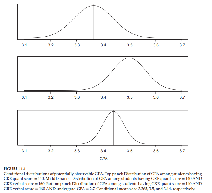
Hans is applying for graduate school at Calisota Tech University (CTU). He sends CTU his quantitative score on the GRE entrance examination $\left(X_1=140\right)$, his verbal score on the $\operatorname{GRE}\left(X_2=160\right)$, and his undergraduate GPA $\left(X_3=2.7\right)$. What would be his final graduate GPA at CTU?

Of course, no one can say. But what we do know, from the Law of Total Variance discussed in Chapter 6, is that the variance of the conditional distribution of $Y=$ final CTU GPA is smaller on average when you consider additional variables. Specifically,
$$
\mathrm{E}\left{\operatorname{Var}\left(Y \mid X_1, X_2, X_3\right)\right} \leq \mathrm{E}\left{\operatorname{Var}\left(Y \mid X_1, X_2\right)\right} \leq \mathrm{E}\left{\operatorname{Var}\left(Y \mid X_1\right)\right}
$$

Figure 11.1 shows how these inequalities might appear, as they relate to Hans. The variation in potentially observable GPAs among students who are like Hans in that they have GRE Math $=140$ is shown in the top panel. Some of that variation is explained by different verbal abilities among students, and the second panel removes that source of variation by considering GPA variation among students who, like Hans, have GRE Math $=140$, and GRE Verbal $=160$. But some of that variation is explained by the general student diligence. Assuming undergraduate GPA is a reasonable measure of such “diligence,” the final panel removes that source of variation by considering GPA variation among students who, like Hans, have GRE Math $=140$, and GRE verbal $=160$, and undergrad GPA $=2.7$. Of course, this can go on and on if additional variables were available, with each additional variable removing a source of variation, leading to distributions with smaller and smaller variances.

The means of the distributions shown in Figure 11.1 are $3.365,3.5$, and 3.44 , respectively. If you were to use one of the distributions to predict Hans, which one would you pick? Clearly, you should pick the one with the smallest variance. His ultimate GPA will be the same number under all three distributions, and since the third distribution has the smallest variance, his GPA will likely be closer to its mean (3.44) than to the other distribution means (3.365 or 3.5).

统计代写|回归分析作业代写Regression Analysis代考|STAT311

回归分析代写

统计代写|回归分析作业代写Regression Analysis代考|The Independence Assumption and Repeated Measurements

你知道吗?在主体/指标变量模型之前,我们对慈善捐款所做的所有分析都是严重错误的,因为独立性假设被严重违反了。你可以毫无疑问地假设,这47个纳税人是相互独立的。但你可能不会认为,对某一特定纳税人的反复观察是独立的。同一纳税人不同年度的慈善行为相似;也就是说,观测结果是依赖的,而不是独立的。假设数据集中有470个独立的观测值是错误的。正如您所记得的,标准误差公式的分母中有一个“$n$”,因此使用$n=470$还是$n=47$有很大的不同。特别是,在上述分析之前,所有模型的标准误差都太小。

很抱歉!我们早就警告过你们,所有这些分析都是有问题的,但我们还需要说明其他几点。这些都是有效点在观察是独立的情况下,所以请不要忘记你学过的东西。
但是现在您知道了,请意识到您必须仔细考虑依赖性问题。你不能,也不应该,把重复的观察看作是独立的。当你假设独立时所有的标准误差都是非常不正确的;理解这个问题的最简单方法是认识到$n=470$与$n=47$有很大的不同。
困惑了吗?模拟救援!下面的R代码模拟和分析了有3个受试者的数据,每个受试者有100个重复,并且每个受试者的数据具有很强的相关性(相似性)。
$$
\begin{aligned}
& \mathrm{s}=3 \quad # \text { subjects } \
& r=100 \quad # \text { replications within subject } \
& \mathrm{X}=\operatorname{rnorm}(\mathrm{s}) ; \mathrm{X}=\operatorname{rep}(\mathrm{X}, \text { each }=r) \text { +rnorm }\left(r^{\star} s, 0, .001\right) \
& \mathrm{a}=\operatorname{rnorm}(\mathrm{s}) ; \mathrm{a}=\operatorname{rep}(\mathrm{a}, \text { each }=r)
\end{aligned}
$$

$e=\operatorname{rnorm}(s \star r, 0, .001)$
$=\mathrm{a}+\mathrm{e}$
$\mathrm{Y}=0+0 \star \mathrm{X}+\operatorname{rnorm}\left(\mathrm{S}^* \mathrm{r}\right)$ tempsilon # $\mathrm{Y}$与$\mathrm{X}$无关
子$=\operatorname{rep}(1: s$,每个$=r)$
总结$(\operatorname{lm}(\mathrm{Y} \sim \mathrm{X}))$ #高度显著$\mathrm{X}$效应
$\operatorname{summary}(\operatorname{lm}(\mathrm{Y} \sim \mathrm{X}+$ as。因子$($ sub $)))$ #不显著$\mathrm{X}$效应

统计代写|回归分析作业代写Regression Analysis代考|Predicting Hans’ Graduate GPA: Theory Versus Practice

汉斯正在申请加州理工大学(CTU)的研究生院。他把GRE入学考试的定量成绩$\left(X_1=140\right)$、口头成绩$\operatorname{GRE}\left(X_2=160\right)$和本科GPA $\left(X_3=2.7\right)$发给CTU。他在CTU毕业时的平均绩点是多少?

当然,谁也说不准。但是我们确实知道,从第6章讨论的总方差定律,当你考虑额外的变量时,$Y=$最终CTU GPA的条件分布的方差平均较小。具体来说,
$$
\mathrm{E}\left{\operatorname{Var}\left(Y \mid X_1, X_2, X_3\right)\right} \leq \mathrm{E}\left{\operatorname{Var}\left(Y \mid X_1, X_2\right)\right} \leq \mathrm{E}\left{\operatorname{Var}\left(Y \mid X_1\right)\right}
$$

图11.1显示了这些不平等在与Hans相关时可能出现的情况。像汉斯一样有GRE数学$=140$的学生的潜在可观察到的gpa的变化显示在顶部的面板中。这种差异的部分原因是学生的语言表达能力不同,第二个小组通过考虑像汉斯这样有GRE数学$=140$和GRE语言$=160$的学生的GPA差异,消除了这种差异的来源。但这种差异的一部分可以用学生的勤奋程度来解释。假设本科GPA是衡量这种“勤奋”的一个合理标准,那么最后的小组就会考虑像汉斯这样拥有GRE数学$=140$、GRE语言$=160$和本科GPA $=2.7$的学生的GPA差异,从而消除这种差异的来源。当然,如果有额外的变量可用,这种情况还会继续下去,每个额外的变量都会消除一个变异源,导致方差越来越小的分布。

图11.1所示分布的均值分别为$3.365,3.5$和3.44。如果你要用其中一个分布来预测汉斯,你会选哪个?显然,你应该选择方差最小的那个。他的最终GPA在所有三个分布下都是相同的数字,并且由于第三个分布的方差最小,他的GPA可能更接近其平均值(3.44),而不是另一个分布的平均值(3.365或3.5)。

统计代写|回归分析作业代写Regression Analysis代考 请认准statistics-lab™

统计代写请认准statistics-lab™. statistics-lab™为您的留学生涯保驾护航。

微观经济学代写

微观经济学是主流经济学的一个分支,研究个人和企业在做出有关稀缺资源分配的决策时的行为以及这些个人和企业之间的相互作用。my-assignmentexpert™ 为您的留学生涯保驾护航 在数学Mathematics作业代写方面已经树立了自己的口碑, 保证靠谱, 高质且原创的数学Mathematics代写服务。我们的专家在图论代写Graph Theory代写方面经验极为丰富,各种图论代写Graph Theory相关的作业也就用不着 说。

线性代数代写

线性代数是数学的一个分支,涉及线性方程,如:线性图,如:以及它们在向量空间和通过矩阵的表示。线性代数是几乎所有数学领域的核心。

博弈论代写

现代博弈论始于约翰-冯-诺伊曼(John von Neumann)提出的两人零和博弈中的混合策略均衡的观点及其证明。冯-诺依曼的原始证明使用了关于连续映射到紧凑凸集的布劳威尔定点定理,这成为博弈论和数学经济学的标准方法。在他的论文之后,1944年,他与奥斯卡-莫根斯特恩(Oskar Morgenstern)共同撰写了《游戏和经济行为理论》一书,该书考虑了几个参与者的合作游戏。这本书的第二版提供了预期效用的公理理论,使数理统计学家和经济学家能够处理不确定性下的决策。

微积分代写

微积分,最初被称为无穷小微积分或 “无穷小的微积分”,是对连续变化的数学研究,就像几何学是对形状的研究,而代数是对算术运算的概括研究一样。

它有两个主要分支,微分和积分;微分涉及瞬时变化率和曲线的斜率,而积分涉及数量的累积,以及曲线下或曲线之间的面积。这两个分支通过微积分的基本定理相互联系,它们利用了无限序列和无限级数收敛到一个明确定义的极限的基本概念 。

计量经济学代写

什么是计量经济学?
计量经济学是统计学和数学模型的定量应用,使用数据来发展理论或测试经济学中的现有假设,并根据历史数据预测未来趋势。它对现实世界的数据进行统计试验,然后将结果与被测试的理论进行比较和对比。

根据你是对测试现有理论感兴趣,还是对利用现有数据在这些观察的基础上提出新的假设感兴趣,计量经济学可以细分为两大类:理论和应用。那些经常从事这种实践的人通常被称为计量经济学家。

Matlab代写

MATLAB 是一种用于技术计算的高性能语言。它将计算、可视化和编程集成在一个易于使用的环境中,其中问题和解决方案以熟悉的数学符号表示。典型用途包括:数学和计算算法开发建模、仿真和原型制作数据分析、探索和可视化科学和工程图形应用程序开发,包括图形用户界面构建MATLAB 是一个交互式系统,其基本数据元素是一个不需要维度的数组。这使您可以解决许多技术计算问题,尤其是那些具有矩阵和向量公式的问题,而只需用 C 或 Fortran 等标量非交互式语言编写程序所需的时间的一小部分。MATLAB 名称代表矩阵实验室。MATLAB 最初的编写目的是提供对由 LINPACK 和 EISPACK 项目开发的矩阵软件的轻松访问,这两个项目共同代表了矩阵计算软件的最新技术。MATLAB 经过多年的发展,得到了许多用户的投入。在大学环境中,它是数学、工程和科学入门和高级课程的标准教学工具。在工业领域,MATLAB 是高效研究、开发和分析的首选工具。MATLAB 具有一系列称为工具箱的特定于应用程序的解决方案。对于大多数 MATLAB 用户来说非常重要,工具箱允许您学习应用专业技术。工具箱是 MATLAB 函数(M 文件)的综合集合,可扩展 MATLAB 环境以解决特定类别的问题。可用工具箱的领域包括信号处理、控制系统、神经网络、模糊逻辑、小波、仿真等。

R语言代写问卷设计与分析代写
PYTHON代写回归分析与线性模型代写
MATLAB代写方差分析与试验设计代写
STATA代写机器学习/统计学习代写
SPSS代写计量经济学代写
EVIEWS代写时间序列分析代写
EXCEL代写深度学习代写
SQL代写各种数据建模与可视化代写

统计代写|回归分析作业代写Regression Analysis代考|The Quadratic Model in Two or More $X$ Variables

如果你也在 怎样代写回归分析Regression Analysis 这个学科遇到相关的难题,请随时右上角联系我们的24/7代写客服。回归分析Regression Analysis回归中的概率观点具体体现在给定X数据的特定固定值的Y数据的可变性模型中。这种可变性是用条件分布建模的;因此,副标题是:“条件分布方法”。回归的整个主题都是用条件分布来表达的;这种观点统一了不同的方法,如经典回归、方差分析、泊松回归、逻辑回归、异方差回归、分位数回归、名义Y数据模型、因果模型、神经网络回归和树回归。所有这些都可以方便地用给定特定X值的Y条件分布模型来看待。

回归分析Regression Analysis条件分布是回归数据的正确模型。它们告诉你,对于变量X的给定值,可能存在可观察到的变量Y的分布。如果你碰巧知道这个分布,那么你就知道了你可能知道的关于响应变量Y的所有信息,因为它与预测变量X的给定值有关。与基于R^2统计量的典型回归方法不同,该模型解释了100%的潜在可观察到的Y数据,后者只解释了Y数据的一小部分,而且在假设几乎总是被违反的情况下也是不正确的。

statistics-lab™ 为您的留学生涯保驾护航 在代写回归分析Regression Analysis方面已经树立了自己的口碑, 保证靠谱, 高质且原创的统计Statistics代写服务。我们的专家在代写回归分析Regression Analysis代写方面经验极为丰富,各种代写回归分析Regression Analysis相关的作业也就用不着说。

统计代写|回归分析作业代写Regression Analysis代考|Parameter Interpretation in Interaction Models

统计代写|回归分析作业代写Regression Analysis代考|The Quadratic Model in Two or More $X$ Variables

The general quadratic response surface as given in the introduction to this chapter is $f\left(x_1, x_2\right)=\beta_0+\beta_1 x_1+\beta_2 x_1^2+\beta_3 x_2+\beta_4 x_2^2+\beta_5 x_1 x_2$. An example for particular choices of the coefficients $\beta$ is shown in Figure 9.3. Notice that the response function is curved, not planar, and is, therefore, more realistic. The term “response surface” is sometimes used instead of “response function” in the case of two or more $X$ variables; the “surface” term is explained by the appearance of the graph of the function in Figure 9.3.
In addition to modeling and testing for curvature in higher dimensional space, quadratic models are also useful for identifying an optimal combination of $X$ values that maximizes or minimizes the response function; see the “rsm” package of $\mathrm{R}$ for more information. While quadratic models are more flexible (and therefore more realistic) than planar models, they can have poor extrapolation properties and are often less realistic than the similarly flexible, curved class of response surfaces known as neural network regression models. In Chapter 17, we compare polynomial regression models with neural network regression models.

统计代写|回归分析作业代写Regression Analysis代考|Interaction (or Moderator) Analysis

The commonly-used interaction model is a special case of the general quadratic model, involving the interaction term but no quadratic terms. When performing interaction analysis, you typically will assume the following conditional mean function:
$$
\mathrm{E}\left(Y \mid X_1=x_1, X_2=x_2\right)=\beta_0+\beta_1 x_1+\beta_2 x_2+\beta_3 x_1 x_2
$$
A slight modification of the Product Complexity example provides a case study in which interaction is needed. Suppose you measure $Y=$ Intent to Purchase a Luxury Product, say expensive jewelry, using a survey of consumers. You also measure the attractiveness $\left(X_1\right)$ of a web design used to display and promote the product, say measured in a scale from 1 to 10 , with $10=$ most attractive design, and the person’s income $\left(X_2\right)$ in a scale from 1 to 5 , with $5=$ most wealthy.

Figure 9.4 shows an example of how this conditional mean function might look. Like the quadratic response surface, it is a curved function in space, not a plane. But note in particular that the effect of $X_1$, Attractiveness of Web Design, on $Y=$ Intent to Purchase, depends on the value of $X_2$, Income: For consumers with the lowest income, $X_2=1$, the slice of the surface corresponding to $X_2=1$ is nearly flat as a function of $X_1=$ Attractiveness of Web Design. That is to say, for people with the lowest income, Attractiveness of Web Design has little effect on Intent to Purchase this luxury product. No surprise! They do not have enough money to purchase luxury items, so the web design is mostly irrelevant to them. On the other hand, for people with the highest income $\left(X_2=5\right)$, the slice of the surface corresponding to $X_2=5$ increases substantially as a function of $X_1=$ Attractiveness of Web Design. Thus, this single model states both (i) that Attractiveness of Web Design $\left(X_1\right)$ has little effect on Intention to Purchase a Luxury Product for people with little money, and (ii) that Attractiveness of Web Design $\left(X_1\right)$ has a substantial effect on Intention to Purchase a Luxury Product for people with lots of money.

统计代写|回归分析作业代写Regression Analysis代考|The Quadratic Model in Two or More $X$ Variables

回归分析代写

统计代写|回归分析作业代写Regression Analysis代考|The Quadratic Model in Two or More $X$ Variables

本章导言中给出的一般二次响应面是$f\left(x_1, x_2\right)=\beta_0+\beta_1 x_1+\beta_2 x_1^2+\beta_3 x_2+\beta_4 x_2^2+\beta_5 x_1 x_2$。图9.3显示了系数$\beta$的特定选择示例。请注意,响应函数是弯曲的,而不是平面的,因此更真实。在两个或多个$X$变量的情况下,有时使用术语“响应面”代替“响应函数”;“面”一词由图9.3所示的函数图来解释。
除了对高维空间中的曲率进行建模和测试外,二次模型还可用于识别使响应函数最大化或最小化的$X$值的最佳组合;有关更多信息,请参阅$\mathrm{R}$的“rsm”包。虽然二次模型比平面模型更灵活(因此也更现实),但它们的外推特性很差,而且往往不如类似灵活的曲线响应面(即神经网络回归模型)真实。在第17章中,我们比较了多项式回归模型和神经网络回归模型。

统计代写|回归分析作业代写Regression Analysis代考|Interaction (or Moderator) Analysis

常用的交互模型是一般二次模型的一种特殊情况,只涉及交互项而不涉及二次项。在进行交互分析时,您通常会假设以下条件平均函数:
$$
\mathrm{E}\left(Y \mid X_1=x_1, X_2=x_2\right)=\beta_0+\beta_1 x_1+\beta_2 x_2+\beta_3 x_1 x_2
$$
对Product Complexity示例稍加修改,提供了一个需要交互的案例研究。假设你通过对消费者的调查来衡量$Y=$购买奢侈品的意向,比如昂贵的珠宝。你还测量了用于展示和推广产品的网页设计的吸引力$\left(X_1\right)$,比如用1到10的等级来衡量,$10=$是最吸引人的设计,而这个人的收入$\left(X_2\right)$用1到5的等级来衡量,$5=$是最富有的。

图9.4显示了这个条件平均函数的示例。和二次响应曲面一样,它是空间中的一个曲线函数,而不是一个平面。但要特别注意的是,$X_1$网页设计吸引力对$Y=$购买意愿的影响取决于$X_2$收入的值:对于收入最低的$X_2=1$消费者来说,$X_2=1$对应的表面片几乎是平坦的,作为$X_1=$网页设计吸引力的函数。也就是说,对于收入最低的人群来说,网页设计的吸引力对购买这一奢侈品的意愿影响不大。一点也不奇怪!他们没有足够的钱去购买奢侈品,所以网页设计基本上与他们无关。另一方面,对于收入最高的人$\left(X_2=5\right)$,对应于$X_2=5$的表面的切片作为$X_1=$的函数显著增加。因此,这个单一的模型表明(i)网页设计的吸引力$\left(X_1\right)$对没有钱的人购买奢侈品的意愿影响很小,(ii)网页设计的吸引力$\left(X_1\right)$对有钱的人购买奢侈品的意愿有实质性的影响。

统计代写|回归分析作业代写Regression Analysis代考 请认准statistics-lab™

统计代写请认准statistics-lab™. statistics-lab™为您的留学生涯保驾护航。

R语言代写问卷设计与分析代写
PYTHON代写回归分析与线性模型代写
MATLAB代写方差分析与试验设计代写
STATA代写机器学习/统计学习代写
SPSS代写计量经济学代写
EVIEWS代写时间序列分析代写
EXCEL代写深度学习代写
SQL代写各种数据建模与可视化代写

统计代写|回归分析作业代写Regression Analysis代考|The Adjusted R-Squared Statistic

如果你也在 怎样代写回归分析Regression Analysis 这个学科遇到相关的难题,请随时右上角联系我们的24/7代写客服。回归分析Regression Analysis回归中的概率观点具体体现在给定X数据的特定固定值的Y数据的可变性模型中。这种可变性是用条件分布建模的;因此,副标题是:“条件分布方法”。回归的整个主题都是用条件分布来表达的;这种观点统一了不同的方法,如经典回归、方差分析、泊松回归、逻辑回归、异方差回归、分位数回归、名义Y数据模型、因果模型、神经网络回归和树回归。所有这些都可以方便地用给定特定X值的Y条件分布模型来看待。

回归分析Regression Analysis条件分布是回归数据的正确模型。它们告诉你,对于变量X的给定值,可能存在可观察到的变量Y的分布。如果你碰巧知道这个分布,那么你就知道了你可能知道的关于响应变量Y的所有信息,因为它与预测变量X的给定值有关。与基于R^2统计量的典型回归方法不同,该模型解释了100%的潜在可观察到的Y数据,后者只解释了Y数据的一小部分,而且在假设几乎总是被违反的情况下也是不正确的。

statistics-lab™ 为您的留学生涯保驾护航 在代写回归分析Regression Analysis方面已经树立了自己的口碑, 保证靠谱, 高质且原创的统计Statistics代写服务。我们的专家在代写回归分析Regression Analysis代写方面经验极为丰富,各种代写回归分析Regression Analysis相关的作业也就用不着说。

统计代写|回归分析作业代写Regression Analysis代考|The Adjusted R-Squared Statistic

统计代写|回归分析作业代写Regression Analysis代考|The Adjusted R-Squared Statistic

Recall that, in the classical model, $\Omega^2=1-\sigma^2 / \sigma_Y^2$, and that the standard $R^2$ statistic replaces the two variances with their maximum likelihood estimates. Recall also that maximum likelihood estimates of variance are biased. With a larger number of predictor variables (i.e., larger $k$ ), the estimate $\hat{\sigma}^2=$ SSE $/ n$ becomes increasingly biased downward, implying in turn that the ordinary $R^2$ becomes increasingly biased upward.
Replacing the two variances with their unbiased estimates gives the adjusted $R^2$ statistic:
$$
R_a^2=1-{\mathrm{SSE} /(n-k-1)} /{\mathrm{SST} /(n-1)}
$$
The adjusted $R^2$ statistic is still biased as an estimator of $\Omega^2=1-\sigma^2 / \sigma_Y^2$ because of Jensen’s inequality, but it is less biased than the ordinary $R^2$ statistic. You can interpret the adjusted $R^2$ statistic in the same way as the ordinary one.

Which estimate is best, adjusted $R^2$ or ordinary $R^2$ ? You guessed it: Use simulation to find out. Despite its reduced bias, the adjusted $R^2$ is not necessarily closer to the true $\Omega^2$, as simulations will show. In addition, the adjusted $R^2$ statistic can be less than 0.0 , which is clearly undesirable. The ordinary $R^2$, like the estimand $\Omega^2$, always lies between 0 and 1 (inclusive).
The following $R$ code locates these $R^2$ statistics in the $1 \mathrm{~m}$ output, and computes them “by hand” as well, using the model where Car Sales is predicted using a quadratic function of Interest Rate.

统计代写|回归分析作业代写Regression Analysis代考|The $F$ Test

See the $\mathrm{R}$ output a few lines above: Underneath the $R^2$ statistic is the $F$-statistic. This statistic is related to the $R^2$ statistic in that it is also a function of SST and SSE (review Figure 8.2). It is given by
$$
F={(\mathrm{SST}-\mathrm{SSE}) / k} /{\mathrm{SSE} /(n-k-1)}
$$
If you add the line ((SST-SSE)/2)/(SSE/(n-3)) to the $\mathrm{R}$ code above, you will get the reported $F$-statistic, although with more decimals: 62.21945.

With a little algebra, you can relate the $F$-statistic directly to the $R^2$ statistic, showing that for fixed $k$ and $n$, larger $R^2$ corresponds to larger $F$ :
$$
F={(n-k-1) / k} \times R^2 /\left(1-R^2\right)
$$
Self-study question: Why is the equation relating $F$ to $R^2$ true?
The $F$-statistic is used to test the global null hypothesis $\mathrm{H}0: \beta_1=\beta_2=\ldots=\beta_k=0$, which states that none of the regression variables $X_1, X_2, \ldots$, or $X_k$ is related to $Y$. Under the classical model where $\mathrm{H}_0: \beta_1=\beta_2=\ldots=\beta_k=0$ is true, the $F$-statistic has a precise and well-known distribution. Distribution of the $F$-statistic under the classical model where $\beta_1=\beta_2=\ldots=\beta_k=0$ $$ F \sim F{k, n-k-1}
$$
where $F_{k, n-k-1}$ is the $F$ distribution with $k$ numerator degrees of freedom and $n-k-1$ denominator degrees of freedom.

统计代写|回归分析作业代写Regression Analysis代考|The Adjusted R-Squared Statistic

回归分析代写

统计代写|回归分析作业代写Regression Analysis代考|The Adjusted R-Squared Statistic

回想一下,在经典模型$\Omega^2=1-\sigma^2 / \sigma_Y^2$中,标准$R^2$统计量用它们的最大似然估计替换了两个方差。还记得方差的最大似然估计是有偏的。随着预测变量数量的增加(即$k$的增大),估计的$\hat{\sigma}^2=$ SSE $/ n$越来越偏向于向下,这反过来意味着普通的$R^2$越来越偏向于向上。
用它们的无偏估计值替换这两个方差,得到调整后的$R^2$统计量:
$$
R_a^2=1-{\mathrm{SSE} /(n-k-1)} /{\mathrm{SST} /(n-1)}
$$
由于Jensen不等式,调整后的$R^2$统计量作为$\Omega^2=1-\sigma^2 / \sigma_Y^2$的估计量仍然有偏倚,但它比普通的$R^2$统计量偏倚小。您可以用与普通统计数据相同的方式解释调整后的$R^2$统计数据。

哪一个估计是最好的,调整$R^2$还是普通$R^2$ ?你猜对了:用模拟来找出答案。尽管偏差减少了,但调整后的$R^2$并不一定更接近真实的$\Omega^2$,正如模拟将显示的那样。此外,调整后的$R^2$统计值可能小于0.0,这显然是不希望看到的。普通的$R^2$和估计的$\Omega^2$一样,总是在0和1之间(含0和1)。
下面的$R$代码在$1 \mathrm{~m}$输出中找到这些$R^2$统计数据,并使用使用利率的二次函数预测汽车销售的模型“手工”计算它们。

统计代写|回归分析作业代写Regression Analysis代考|The $F$ Test

请参阅上面几行$\mathrm{R}$输出:$R^2$统计数据下面是$F$ -统计数据。该统计量与$R^2$统计量相关,因为它也是SST和SSE的函数(参见图8.2)。它是由
$$
F={(\mathrm{SST}-\mathrm{SSE}) / k} /{\mathrm{SSE} /(n-k-1)}
$$
如果在上面的$\mathrm{R}$代码中添加((SST-SSE)/2)/(SSE/(n-3))行,您将得到报告的$F$ -统计数据,尽管有更多的小数:62.21945。

使用一点代数,您可以将$F$ -统计直接与$R^2$统计关联起来,表明对于固定的$k$和$n$,较大的$R^2$对应较大的$F$:
$$
F={(n-k-1) / k} \times R^2 /\left(1-R^2\right)
$$
自习题:为什么$F$和$R^2$的等式是正确的?
$F$ -统计量用于检验全局零假设$\mathrm{H}0: \beta_1=\beta_2=\ldots=\beta_k=0$,它表明回归变量$X_1, X_2, \ldots$或$X_k$都与$Y$无关。在$\mathrm{H}0: \beta_1=\beta_2=\ldots=\beta_k=0$为真的经典模型下,$F$ -统计量具有精确且众所周知的分布。经典模型下$F$ -统计量的分布,其中$\beta_1=\beta_2=\ldots=\beta_k=0$$$ F \sim F{k, n-k-1} $$ 其中$F{k, n-k-1}$为分子自由度为$k$,分母自由度为$n-k-1$的$F$分布。

统计代写|回归分析作业代写Regression Analysis代考 请认准statistics-lab™

统计代写请认准statistics-lab™. statistics-lab™为您的留学生涯保驾护航。

R语言代写问卷设计与分析代写
PYTHON代写回归分析与线性模型代写
MATLAB代写方差分析与试验设计代写
STATA代写机器学习/统计学习代写
SPSS代写计量经济学代写
EVIEWS代写时间序列分析代写
EXCEL代写深度学习代写
SQL代写各种数据建模与可视化代写

统计代写|回归分析作业代写Regression Analysis代考|Multiple Regression from the Matrix Point of View

如果你也在 怎样代写回归分析Regression Analysis 这个学科遇到相关的难题,请随时右上角联系我们的24/7代写客服。回归分析Regression Analysis回归中的概率观点具体体现在给定X数据的特定固定值的Y数据的可变性模型中。这种可变性是用条件分布建模的;因此,副标题是:“条件分布方法”。回归的整个主题都是用条件分布来表达的;这种观点统一了不同的方法,如经典回归、方差分析、泊松回归、逻辑回归、异方差回归、分位数回归、名义Y数据模型、因果模型、神经网络回归和树回归。所有这些都可以方便地用给定特定X值的Y条件分布模型来看待。

回归分析Regression Analysis条件分布是回归数据的正确模型。它们告诉你,对于变量X的给定值,可能存在可观察到的变量Y的分布。如果你碰巧知道这个分布,那么你就知道了你可能知道的关于响应变量Y的所有信息,因为它与预测变量X的给定值有关。与基于R^2统计量的典型回归方法不同,该模型解释了100%的潜在可观察到的Y数据,后者只解释了Y数据的一小部分,而且在假设几乎总是被违反的情况下也是不正确的。

statistics-lab™ 为您的留学生涯保驾护航 在代写回归分析Regression Analysis方面已经树立了自己的口碑, 保证靠谱, 高质且原创的统计Statistics代写服务。我们的专家在代写回归分析Regression Analysis代写方面经验极为丰富,各种代写回归分析Regression Analysis相关的作业也就用不着说。

统计代写|回归分析作业代写Regression Analysis代考|Multiple Regression from the Matrix Point of View

统计代写|回归分析作业代写Regression Analysis代考|Multiple Regression from the Matrix Point of View

In the case of simple regression, you saw that the OLS estimate of slope has a simple form: It is the estimated covariance of the $(X, Y)$ distribution, divided by the estimated variance of the $X$ distribution, or $\hat{\beta}1=\hat{\sigma}{x y} / \hat{\sigma}_x^2$. There is no such simple formula in multiple regression. Instead, you must use matrix algebra, involving matrix multiplication and matrix inverses. If you are unfamiliar with basic matrix algebra, including multiplication, addition, subtraction, transpose, identity matrix, and matrix inverse, you should take some time now to get acquainted with those particular concepts before reading on. (Perhaps you can locate a “matrix algebra for beginners” type of web page.)
Done? Ok, read on.
Our first use of matrix algebra in regression is to give a concise representation of the regression model. Multiple regression models refer to $n$ observations and $k$ variables, both of which can be in the thousands or even millions. The following matrix form of the model provides a very convenient shorthand to represent all this information.
$$
Y=\mathrm{X} \beta+\varepsilon
$$
This concise form covers all the $n$ observations and all the $X$ variables ( $k$ of them) in one simple equation. Note that there are boldface non-italic terms and boldface italic terms in the expression. To make the material easier to read, we use the convention that boldface means a matrix, while boldface italic refers to a vector, which is a matrix with a single column. Thus $\boldsymbol{Y}, \boldsymbol{\beta}$, and $\varepsilon$, are vectors (single-column matrices), while $\mathbf{X}$ is a matrix having multiple columns.

统计代写|回归分析作业代写Regression Analysis代考|The Least Squares Estimates in Matrix Form

One use of matrix algebra is to display the model for all $n$ observations and all $X$ variables succinctly as shown above. Another use is to identify the OLS estimates of the $\beta$ ‘s. There is simply no way to display the OLS estimates other than by using matrix algebra, as follows:
$$
\hat{\boldsymbol{\beta}}=\left(\mathbf{X}^{\mathrm{T}} \mathbf{X}\right)^{-1} \mathbf{X}^{\mathrm{T}} Y
$$
(The ” $\mathrm{T}$ ” symbol denotes transpose of the matrix.) To see why the OLS estimates have this matrix representation, recall that in the simple, classical regression model, the maximum likelihood (ML) estimates must minimize the sum of squared “errors” called SSE. The same is true in multiple regression: The ML estimates must minimize the function
$$
\operatorname{SSE}\left(\beta_0, \beta_1, \ldots, \beta_k\right)=\sum_{i=1}^n\left{y_i-\left(\beta_0+\beta_1 x_{i 1}+\cdots+\beta_k x_{i k}\right)\right}^2
$$

In the case of two $X$ variables $(k=2)$, you are to choose $\hat{\beta}0, \hat{\beta}_1$, and $\hat{\beta}_2$ that define the plane, $f\left(x_1, x_2\right)=\hat{\beta}_0+\hat{\beta}_1 x_1+\hat{\beta}_2 x_2$, such as the one shown in Figure 6.3 , that minimizes the sum of squared vertical deviations from the 3-dimensional point cloud $\left(x{i 1}, x_{i 2}, y_i\right), i=1,2, \ldots, n$. Figure 7.1 illustrates the concept.

统计代写|回归分析作业代写Regression Analysis代考|Multiple Regression from the Matrix Point of View

回归分析代写

统计代写|回归分析作业代写Regression Analysis代考|Multiple Regression from the Matrix Point of View

在简单回归的情况下,您看到斜率的OLS估计有一个简单的形式:它是$(X, Y)$分布的估计协方差除以$X$分布或$\hat{\beta}1=\hat{\sigma}{x y} / \hat{\sigma}_x^2$的估计方差。在多元回归中没有这样简单的公式。相反,你必须使用矩阵代数,包括矩阵乘法和矩阵逆。如果您不熟悉基本的矩阵代数,包括乘法、加法、减法、转置、单位矩阵和矩阵逆,那么在继续阅读之前,您应该花一些时间熟悉这些特定的概念。(也许你可以找到一个“矩阵代数初学者”类型的网页。)
搞定了?好吧,继续读下去。
我们在回归中首先使用矩阵代数是为了给出回归模型的简明表示。多元回归模型涉及$n$观测值和$k$变量,这两个变量都可以是数千甚至数百万。该模型的以下矩阵形式提供了一种非常方便的速记方式来表示所有这些信息。
$$
Y=\mathrm{X} \beta+\varepsilon
$$
这个简洁的形式在一个简单的方程中涵盖了所有的$n$观测值和所有的$X$变量(其中的$k$变量)。请注意,表达式中有黑体非斜体项和黑体斜体项。为了使材料更容易阅读,我们使用约定,黑体表示矩阵,而黑体斜体表示向量,这是一个具有单列的矩阵。因此$\boldsymbol{Y}, \boldsymbol{\beta}$和$\varepsilon$是向量(单列矩阵),而$\mathbf{X}$是具有多列的矩阵。

统计代写|回归分析作业代写Regression Analysis代考|The Least Squares Estimates in Matrix Form

矩阵代数的一种用法是简洁地显示所有$n$观测值和所有$X$变量的模型,如上所示。另一个用途是识别$\beta$的OLS估计。除了使用矩阵代数之外,根本没有办法显示OLS估计,如下所示:
$$
\hat{\boldsymbol{\beta}}=\left(\mathbf{X}^{\mathrm{T}} \mathbf{X}\right)^{-1} \mathbf{X}^{\mathrm{T}} Y
$$
(“$\mathrm{T}$”符号表示矩阵的转置。)要了解为什么OLS估计具有这种矩阵表示,请回忆一下,在简单的经典回归模型中,最大似然(ML)估计必须最小化称为SSE的平方“误差”的总和。在多元回归中也是如此:机器学习估计必须最小化函数
$$
\operatorname{SSE}\left(\beta_0, \beta_1, \ldots, \beta_k\right)=\sum_{i=1}^n\left{y_i-\left(\beta_0+\beta_1 x_{i 1}+\cdots+\beta_k x_{i k}\right)\right}^2
$$

在有两个$X$变量$(k=2)$的情况下,您将选择$\hat{\beta}0, \hat{\beta}1$和$\hat{\beta}_2$来定义平面$f\left(x_1, x_2\right)=\hat{\beta}_0+\hat{\beta}_1 x_1+\hat{\beta}_2 x_2$,如图6.3所示,它最小化与三维点云$\left(x{i 1}, x{i 2}, y_i\right), i=1,2, \ldots, n$垂直偏差的平方和。图7.1说明了这个概念。

统计代写|回归分析作业代写Regression Analysis代考 请认准statistics-lab™

统计代写请认准statistics-lab™. statistics-lab™为您的留学生涯保驾护航。

R语言代写问卷设计与分析代写
PYTHON代写回归分析与线性模型代写
MATLAB代写方差分析与试验设计代写
STATA代写机器学习/统计学习代写
SPSS代写计量经济学代写
EVIEWS代写时间序列分析代写
EXCEL代写深度学习代写
SQL代写各种数据建模与可视化代写

统计代写|回归分析作业代写Regression Analysis代考|Evaluating the Linearity Assumption Using Hypothesis Testing Methods

如果你也在 怎样代写回归分析Regression Analysis这个学科遇到相关的难题,请随时右上角联系我们的24/7代写客服。

回归分析是一种强大的统计方法,允许你检查两个或多个感兴趣的变量之间的关系。虽然有许多类型的回归分析,但它们的核心都是考察一个或多个自变量对因变量的影响。

statistics-lab™ 为您的留学生涯保驾护航 在代写回归分析Regression Analysis方面已经树立了自己的口碑, 保证靠谱, 高质且原创的统计Statistics代写服务。我们的专家在代写回归分析Regression Analysis代写方面经验极为丰富,各种代写回归分析Regression Analysis相关的作业也就用不着说。

统计代写|回归分析作业代写Regression Analysis代考|Evaluating the Linearity Assumption Using Hypothesis Testing Methods

统计代写|回归分析作业代写Regression Analysis代考|Evaluating the Linearity Assumption Using Hypothesis Testing Methods

Here, we will get slightly ahead of the flow of the book, because multiple regression is covered in the next chapter. A simple, powerful way to test for curvature is to use a multiple regression model that includes a quadratic term. The quadratic regression model is given by:
$$
Y=\beta_0+\beta_1 X+\beta_2 X^2+\varepsilon
$$
This model assumes that, if there is curvature, then it takes a quadratic form. Logic for making this assumption is given by “Taylor’s Theorem,” which states that many types of curved functions are well approximated by quadratic functions.

Testing methods require restricted (null) and unrestricted (alternative) models. Here, the null model enforces the restriction that $\beta_2=0$; thus the null model states that the mean response is a linear (not curved) function of $x$. So-called “insignificance” (determined historically by $p>0.05$ ) of the estimate of $\beta_2$ means that the evidence of curvature in the observed data, as indicated by a non-zero estimate of $\beta_2$ or by a curved LOESS fit, is explainable by chance alone under the linear model. “Significance” (determined historically by $p<0.05$ ) means that such evidence of curvature is not easily explained by chance alone under the linear model.

But you should not take the result of this $p$-value based test as a “recipe” for model construction. If “significant,” you should not automatically assume a curved model. Instead, you should ask, “Is the curvature dramatic enough to warrant the additional modeling complexity?” and “Do the predictions differ much, whether you use a model for curvature or the ordinary linear model?” If the answers to those questions are “No,” then you should use the linear model anyway, even if it was “rejected” by the $p$-value based test.

In addition, models employing curvature (particularly quadratics) are notoriously poor at the extremes of the $x$-range(s). So again, you can easily prefer the linear model, even if the curvature is “significant” $(p<0.05)$.

统计代写|回归分析作业代写Regression Analysis代考|Testing for Curvature with the Production Cost Data

The following R code illustrates the method.
ProdC $=$ read.table(“https://raw.githubusercontent.com/andrea2719/
URA-DataSets/master/ProdC.txt”)
attach(ProdC)
plot (Widgets, Cost); abline(lsfit(Widgets, Cost))
Widgets.squared = Widgets^2
Prodc $=$ read.table $($ “https $: / /$ raw.githubusercontent.com/andrea2719/
URA-Datasets/master/ProdC.txt”)
attach (ProdC)
plot (Widgets, Cost); abline(lsfit(Widgets, Cost))
Widgets.squared $=$ Widgets $^{\wedge} 2$

fit.quad $=1 \mathrm{~m}$ (Cost $~$ Widgets + Widgets.squared); summary (fit.quad)
lines(spline(Widgets, predict(fit.quad)), col = “gray”, lty=2)
Figure 4.3 shows both the linear and quadratic (curved) fit to the data. Since the linear and quadratic fits are so similar, it (again) appears that there is no need to model the curvature explicitly in this example.
Relevant lines from the summary of fit are shown as follows:
Coefficients :
(Intercept)
widgets
Widgets.squared
$\begin{array}{cccc}\text { Estimate } & \text { Std. Error } & t \text { value } & \operatorname{Pr}(>|t|) \ 4.564 e+02 & 7.493 e+02 & 0.609 & 0.546 \ 9.149 e-01 & 1.290 e+00 & 0.709 & 0.483 \ 2.923 e-04 & 5.322 e-04 & 0.549 & 0.586\end{array}$
Residual standard error: 241.3 on 37 degrees of freedom
Multiple R-squared: 0.7987 , Adjusted R-squared: 0.7878
F-statistic: 73.42 on 2 and $37 \mathrm{DF}$, p-value: $1.318 \mathrm{e}-13$
Notice the $p$-value for testing the $\beta_2=0$ restriction: Since the $p$-value is 0.586 , the difference between the coefficient 0.0002923 (2.923e-04) and 0.0 is explainable by chance alone. That is, even if the process were truly linear (i.e., even if $\beta_2=0$ ), you would often see quadratic coefficient estimates $\left(\hat{\beta}_2\right)$ as large as 0.0002923 when you fit a quadratic model to similar data. If this is confusing to you, just run a simulation from a similar linear process (where $\beta_2=0$ ), and fit a quadratic model. You will see a non-zero $\hat{\beta}_2$ in every simulated data set, and most will be within 2 standard errors of 0.0 (the $\hat{\beta}_2$ above is $T=0.549$ standard errors from 0.0 ).

统计代写|回归分析作业代写Regression Analysis代考|Evaluating the Linearity Assumption Using Hypothesis Testing Methods

回归分析代写

统计代写|回归分析作业代写Regression Analysis代考|Evaluating the Linearity Assumption Using Hypothesis Testing Methods

在这里,我们将略超前于本书的流程,因为多元回归将在下一章中讨论。测试曲率的一个简单而有力的方法是使用包含二次项的多元回归模型。二次回归模型为:
$$
Y=\beta_0+\beta_1 X+\beta_2 X^2+\varepsilon
$$
这个模型假设,如果存在曲率,那么它是二次型的。做出这种假设的逻辑是由“泰勒定理”给出的,该定理指出,许多类型的曲线函数都可以很好地近似于二次函数。

测试方法需要受限制(null)和不受限制(alternative)的模型。在这里,null模型强制限制$\beta_2=0$;因此,零模型表明平均响应是$x$的线性(而不是曲线)函数。所谓的$\beta_2$估计的“不显著性”(历史上由$p>0.05$确定)意味着观测数据中的曲率证据,如$\beta_2$的非零估计或弯曲的黄土拟合所表明的那样,在线性模型下只能由偶然解释。“重要性”(历史上由$p<0.05$决定)意味着这种曲率的证据在线性模型下不容易单独用偶然来解释。

但是,您不应该将这个基于$p$值的测试的结果作为模型构建的“配方”。如果“重要”,您不应该自动假设一个曲线模型。相反,您应该问:“曲率是否足够大,足以保证额外的建模复杂性?”以及“使用曲率模型还是普通线性模型,预测的差异是否很大?”如果这些问题的答案是“否”,那么无论如何都应该使用线性模型,即使它被基于$p$值的测试“拒绝”。

此外,采用曲率(特别是二次曲线)的模型在$x$ -范围的极值处是出了名的差。所以,你可以很容易地选择线性模型,即使曲率是“显著的”$(p<0.05)$。

统计代写|回归分析作业代写Regression Analysis代考|Testing for Curvature with the Production Cost Data

下面的R代码演示了该方法。
ProdC $=$ read.table(“https://raw.githubusercontent.com/andrea2719/
“ura – dataset /master/ product .txt”)
附件(产品)
plot (Widgets, Cost);abline(lsfit(Widgets, Cost))
小部件。^2 = Widgets^2
产品$=$阅读。表$($ “https $: / /$ raw.githubusercontent.com/andrea2719/
“ura – dataset /master/ product .txt”)
附件(产品)
plot (Widgets, Cost);abline(lsfit(Widgets, Cost))
小部件。squared $=$小部件 $^{\wedge} 2$

适合。quad $=1 \mathrm{~m}$(成本$~$ Widgets + Widgets.squared);总结(fit.quad)
线条(样条(Widgets, predict(fit.quad)), col = “gray”, lty=2)
图4.3显示了数据的线性拟合和二次(曲线)拟合。由于线性拟合和二次拟合是如此相似,它(再次)似乎没有必要在这个例子中明确地建模曲率。
拟合总结的相关行如下:
系数:
(截语)
小部件
widgets。squared
$\begin{array}{cccc}\text { Estimate } & \text { Std. Error } & t \text { value } & \operatorname{Pr}(>|t|) \ 4.564 e+02 & 7.493 e+02 & 0.609 & 0.546 \ 9.149 e-01 & 1.290 e+00 & 0.709 & 0.483 \ 2.923 e-04 & 5.322 e-04 & 0.549 & 0.586\end{array}$
37个自由度的残差标准误差:241.3
多元r平方:0.7987,调整r平方:0.7878
f统计量:73.42对2和$37 \mathrm{DF}$, p值:$1.318 \mathrm{e}-13$
请注意用于测试$\beta_2=0$限制的$p$ -值:由于$p$ -值为0.586,因此系数0.0002923 (2.923e-04)和0.0之间的差异只能通过偶然来解释。也就是说,即使这个过程是真正线性的(即,即使$\beta_2=0$),当您将二次模型拟合到类似的数据时,您经常会看到二次系数估计$\left(\hat{\beta}_2\right)$大到0.0002923。如果这让您感到困惑,只需从类似的线性过程($\beta_2=0$)运行模拟,并拟合二次模型。您将在每个模拟数据集中看到一个非零$\hat{\beta}_2$,并且大多数将在0.0的2个标准误差范围内(上面的$\hat{\beta}_2$是0.0的$T=0.549$标准误差)。

统计代写|回归分析作业代写Regression Analysis代考 请认准statistics-lab™

统计代写请认准statistics-lab™. statistics-lab™为您的留学生涯保驾护航。

随机过程代考

在概率论概念中,随机过程随机变量的集合。 若一随机系统的样本点是随机函数,则称此函数为样本函数,这一随机系统全部样本函数的集合是一个随机过程。 实际应用中,样本函数的一般定义在时间域或者空间域。 随机过程的实例如股票和汇率的波动、语音信号、视频信号、体温的变化,随机运动如布朗运动、随机徘徊等等。

贝叶斯方法代考

贝叶斯统计概念及数据分析表示使用概率陈述回答有关未知参数的研究问题以及统计范式。后验分布包括关于参数的先验分布,和基于观测数据提供关于参数的信息似然模型。根据选择的先验分布和似然模型,后验分布可以解析或近似,例如,马尔科夫链蒙特卡罗 (MCMC) 方法之一。贝叶斯统计概念及数据分析使用后验分布来形成模型参数的各种摘要,包括点估计,如后验平均值、中位数、百分位数和称为可信区间的区间估计。此外,所有关于模型参数的统计检验都可以表示为基于估计后验分布的概率报表。

广义线性模型代考

广义线性模型(GLM)归属统计学领域,是一种应用灵活的线性回归模型。该模型允许因变量的偏差分布有除了正态分布之外的其它分布。

statistics-lab作为专业的留学生服务机构,多年来已为美国、英国、加拿大、澳洲等留学热门地的学生提供专业的学术服务,包括但不限于Essay代写,Assignment代写,Dissertation代写,Report代写,小组作业代写,Proposal代写,Paper代写,Presentation代写,计算机作业代写,论文修改和润色,网课代做,exam代考等等。写作范围涵盖高中,本科,研究生等海外留学全阶段,辐射金融,经济学,会计学,审计学,管理学等全球99%专业科目。写作团队既有专业英语母语作者,也有海外名校硕博留学生,每位写作老师都拥有过硬的语言能力,专业的学科背景和学术写作经验。我们承诺100%原创,100%专业,100%准时,100%满意。

机器学习代写

随着AI的大潮到来,Machine Learning逐渐成为一个新的学习热点。同时与传统CS相比,Machine Learning在其他领域也有着广泛的应用,因此这门学科成为不仅折磨CS专业同学的“小恶魔”,也是折磨生物、化学、统计等其他学科留学生的“大魔王”。学习Machine learning的一大绊脚石在于使用语言众多,跨学科范围广,所以学习起来尤其困难。但是不管你在学习Machine Learning时遇到任何难题,StudyGate专业导师团队都能为你轻松解决。

多元统计分析代考


基础数据: $N$ 个样本, $P$ 个变量数的单样本,组成的横列的数据表
变量定性: 分类和顺序;变量定量:数值
数学公式的角度分为: 因变量与自变量

时间序列分析代写

随机过程,是依赖于参数的一组随机变量的全体,参数通常是时间。 随机变量是随机现象的数量表现,其时间序列是一组按照时间发生先后顺序进行排列的数据点序列。通常一组时间序列的时间间隔为一恒定值(如1秒,5分钟,12小时,7天,1年),因此时间序列可以作为离散时间数据进行分析处理。研究时间序列数据的意义在于现实中,往往需要研究某个事物其随时间发展变化的规律。这就需要通过研究该事物过去发展的历史记录,以得到其自身发展的规律。

回归分析代写

多元回归分析渐进(Multiple Regression Analysis Asymptotics)属于计量经济学领域,主要是一种数学上的统计分析方法,可以分析复杂情况下各影响因素的数学关系,在自然科学、社会和经济学等多个领域内应用广泛。

MATLAB代写

MATLAB 是一种用于技术计算的高性能语言。它将计算、可视化和编程集成在一个易于使用的环境中,其中问题和解决方案以熟悉的数学符号表示。典型用途包括:数学和计算算法开发建模、仿真和原型制作数据分析、探索和可视化科学和工程图形应用程序开发,包括图形用户界面构建MATLAB 是一个交互式系统,其基本数据元素是一个不需要维度的数组。这使您可以解决许多技术计算问题,尤其是那些具有矩阵和向量公式的问题,而只需用 C 或 Fortran 等标量非交互式语言编写程序所需的时间的一小部分。MATLAB 名称代表矩阵实验室。MATLAB 最初的编写目的是提供对由 LINPACK 和 EISPACK 项目开发的矩阵软件的轻松访问,这两个项目共同代表了矩阵计算软件的最新技术。MATLAB 经过多年的发展,得到了许多用户的投入。在大学环境中,它是数学、工程和科学入门和高级课程的标准教学工具。在工业领域,MATLAB 是高效研究、开发和分析的首选工具。MATLAB 具有一系列称为工具箱的特定于应用程序的解决方案。对于大多数 MATLAB 用户来说非常重要,工具箱允许您学习应用专业技术。工具箱是 MATLAB 函数(M 文件)的综合集合,可扩展 MATLAB 环境以解决特定类别的问题。可用工具箱的领域包括信号处理、控制系统、神经网络、模糊逻辑、小波、仿真等。

R语言代写问卷设计与分析代写
PYTHON代写回归分析与线性模型代写
MATLAB代写方差分析与试验设计代写
STATA代写机器学习/统计学习代写
SPSS代写计量经济学代写
EVIEWS代写时间序列分析代写
EXCEL代写深度学习代写
SQL代写各种数据建模与可视化代写

统计代写|回归分析作业代写Regression Analysis代考|Simulation Study to Understand the Null Distribution of the $T$ Statistic

如果你也在 怎样代写回归分析Regression Analysis这个学科遇到相关的难题,请随时右上角联系我们的24/7代写客服。

回归分析是一种强大的统计方法,允许你检查两个或多个感兴趣的变量之间的关系。虽然有许多类型的回归分析,但它们的核心都是考察一个或多个自变量对因变量的影响。

statistics-lab™ 为您的留学生涯保驾护航 在代写回归分析Regression Analysis方面已经树立了自己的口碑, 保证靠谱, 高质且原创的统计Statistics代写服务。我们的专家在代写回归分析Regression Analysis代写方面经验极为丰富,各种代写回归分析Regression Analysis相关的作业也就用不着说。

统计代写|回归分析作业代写Regression Analysis代考|Simulation Study to Understand the Null Distribution of the $T$ Statistic

统计代写|回归分析作业代写Regression Analysis代考|Simulation Study to Understand the Null Distribution of the $T$ Statistic

The following $\mathrm{R}$ code generates the data under the null model. It is the same model used in the SSN/Height example above, but re-written in a way to make the constraint $\beta_1=0$ explicit. Because we did not use set.seed as in the previous code, the output is random. Your results will differ, but that is good because the point here is to understand randomness.

$\mathrm{n}=100$
beta $0=70 ;$ betal $=0 \quad #$ The null model; true betal = 0
ssn = sample $(0: 9,100$, replace=T)
height = beta + betal*ssn + rnorm $(100,0,4)$
ssn.data = data.frame (ssn, height)
fit. $1=$ lm (height ssn, data=ssn.data)
summary (fit. 1$)$
$\mathrm{n}=100$
beta $0=70 ;$ betal $=0 \quad #$ The null model; true betal $=0$
ssn $=$ sample $(0: 9,100$, replace $=T)$
height $=$ beta $0+\operatorname{beta} 1 * \operatorname{ssn}+\operatorname{rnorm}(100,0,4)$
ssn. data = data. frame (ssn, height)
fit. 1 = $\operatorname{lm}($ height ssn, datasssn. data)
summary (fit.l)
This code gives the following output (yours will vary by randomness):
Cal :
$\operatorname{lm}$ (formula $=$ height $\sim$ ssn, data $=$ ssn. data)
Residuals:
Min $1 Q$ Median $3 Q$ Max
$-9.4952-2.8261-0.3936 \quad 2.252111 .6764$
Coefficients :
Estimate std. Error $t$ value $\operatorname{Pr}(>|t|)$
(Intercept) $69.77372 \quad 0.71865 \quad 97.089<2 \mathrm{e}-16 \star \star $ $\operatorname{ssn} 0.019150 .14336 \quad 0.134 \quad 0.894$ Signif. Codes: 0 ‘‘ 0.001 ‘‘ 0.01 ‘*’ 0.05 ‘. 0.1 ‘ 1
Residual standard error: 4.155 on 98 degrees of freedom
Multiple R-squared: 0.000182 , Adjusted R-squared: 0.01002
F-statistic: 0.01784 on 1 and $98 \mathrm{DF}$, p-value: 0.894
In our simulation, the estimate $\hat{\beta}_1=0.01915$ is $T=0.134$ standard errors from zero, and you know that this difference is explained by chance alone because the data are simulated from the null model where $\beta_1=0$.

统计代写|回归分析作业代写Regression Analysis代考|The $p$-Value

In the example above, the thresholds to determine which real $T$ values are explainable by chance alone are the numbers that put $95 \%$ of the $T$ values that are explained by chance alone between them; these are -1.9845 and +1.9845 in the case of the $T_{98}$ distribution. If the observed $T$ statistic falls outside that range, then we can say that the difference between $\hat{\beta}_1$ and 0 is not easily explained by chance alone.

See Figure 3.7 again. Notice that there is $5 \%$ total probability outside the \pm 1.9845 range, simply because there is $95 \%$ probability inside the range. Now, if the $T$ statistic falls inside the $95 \%$ range, then there has to be more than $5 \%$ total probability outside the $\pm T$ range. See Figure 3.7 again, and suppose $T=1.7$, which is inside the range. Then there has to be more than $5 \%$ probability outside the \pm 1.7 range, right? See Figure 3.7 again, and locate \pm 1.7 on the graph. Make sure you understand this; it is not hard at all. Do not just read the words, because then you will not understand. Instead, look at Figure 3.7, put your finger on the graph at 1.7 , and think about the area outside the \pm 1.7 range. It is more than 0.05 , do you see?

Now, suppose $T=2.5$, and look at Figure 3.7 again. Then there has to be less than $5 \%$ probability outside the \pm 2.5 range, right? See Figure 3.7 again, and locate \pm 2.5 on the graph. Make sure you understand this; it is not hard at all. Look at the graph! Do not just read the words! Instead, put your finger on the graph at 2.5 and think about the area outside the \pm 2.5 range. It is less than 0.05 , do you see?

统计代写|回归分析作业代写Regression Analysis代考|Simulation Study to Understand the Null Distribution of the $T$ Statistic

回归分析代写

统计代写|回归分析作业代写Regression Analysis代考|Simulation Study to Understand the Null Distribution of the $T$ Statistic

下面的$\mathrm{R}$代码生成null模型下的数据。它与上面的SSN/Height示例中使用的模型相同,但是以一种使约束$\beta_1=0$显式的方式重新编写。因为我们没有用集合。与前面的代码一样,输出是随机的。你的结果可能会有所不同,但这很好,因为这里的重点是理解随机性。

$\mathrm{n}=100$
beta $0=70 ;$ betal $=0 \quad #$ null模型;True betal = 0
ssn = sample $(0: 9,100$, replace=T)
高度= beta + beta *ssn + rnorm $(100,0,4)$
ssn. ssn.Data = Data .frame (ssn, height)
适合。$1=$ lm(高度ssn,数据=ssn.data)
总结(适合)1 $)$
$\mathrm{n}=100$
beta $0=70 ;$ betal $=0 \quad #$ null模型;真betal $=0$
SSN $=$样例$(0: 9,100$,替换$=T)$
身高$=$ beta $0+\operatorname{beta} 1 * \operatorname{ssn}+\operatorname{rnorm}(100,0,4)$
ssn. ssn.数据=数据。框架(ssn, height)
适合。1 = $\operatorname{lm}($ height ssn, datasssn。数据)
摘要(fit. 1)
这段代码给出了以下输出(你的输出会随随机而变化):
卡尔:
$\operatorname{lm}$(公式$=$高度$\sim$ ssn,数据$=$ ssn。数据)
残差:
最小值$1 Q$中值$3 Q$最大值
$-9.4952-2.8261-0.3936 \quad 2.252111 .6764$
系数:
估计std误差$t$值$\operatorname{Pr}(>|t|)$
(截音)$69.77372 \quad 0.71865 \quad 97.089<2 \mathrm{e}-16 \star \star $$\operatorname{ssn} 0.019150 .14336 \quad 0.134 \quad 0.894$代码:0“0.001”“0.01”*“0.05”。0.1 ‘ 1
剩余标准误差:在98自由度上为4.155
多元r平方:0.000182,调整r平方:0.01002
f统计量:0.01784对1和$98 \mathrm{DF}$, p值:0.894
在我们的模拟中,估计值$\hat{\beta}_1=0.01915$是$T=0.134$离零的标准误差,并且您知道这种差异完全是偶然的,因为数据是从null模型模拟的,其中$\beta_1=0$。

统计代写|回归分析作业代写Regression Analysis代考|The $p$-Value

在上面的例子中,确定哪些真实的$T$值只能由偶然解释的阈值是将只能由偶然解释的$T$值中的$95 \%$放在它们之间的数字;在$T_{98}$分布的情况下,它们是-1.9845和+1.9845。如果观察到的$T$统计值超出了这个范围,那么我们可以说$\hat{\beta}_1$和0之间的差异不容易单独用偶然来解释。

再次参见图3.7。注意,在\pm 1.9845范围之外有$5 \%$总概率,因为在范围内有$95 \%$概率。现在,如果$T$统计值落在$95 \%$范围内,那么在$\pm T$范围外的总概率必须大于$5 \%$。再次参见图3.7,假设$T=1.7$在范围内。那么在\pm 1.7范围之外的概率必须大于$5 \%$,对吧?再次参见图3.7,并在图中找到\pm 1.7。确保你理解了这一点;这一点也不难。不要只看文字,因为那样你不会明白。相反,请查看图3.7,将手指放在1.7处的图形上,并考虑\pm 1.7范围之外的区域。它大于0.05,你看到了吗?

现在,假设$T=2.5$,再次查看图3.7。那么在\pm 2.5范围之外的概率必须小于$5 \%$,对吧?再次参见图3.7,在图中找到\pm 2.5。确保你理解了这一点;这一点也不难。看这个图表!不要只看单词!相反,将手指放在2.5的图形上,并考虑\pm 2.5范围之外的区域。它小于0.05,你看到了吗?

统计代写|回归分析作业代写Regression Analysis代考 请认准statistics-lab™

统计代写请认准statistics-lab™. statistics-lab™为您的留学生涯保驾护航。

随机过程代考

在概率论概念中,随机过程随机变量的集合。 若一随机系统的样本点是随机函数,则称此函数为样本函数,这一随机系统全部样本函数的集合是一个随机过程。 实际应用中,样本函数的一般定义在时间域或者空间域。 随机过程的实例如股票和汇率的波动、语音信号、视频信号、体温的变化,随机运动如布朗运动、随机徘徊等等。

贝叶斯方法代考

贝叶斯统计概念及数据分析表示使用概率陈述回答有关未知参数的研究问题以及统计范式。后验分布包括关于参数的先验分布,和基于观测数据提供关于参数的信息似然模型。根据选择的先验分布和似然模型,后验分布可以解析或近似,例如,马尔科夫链蒙特卡罗 (MCMC) 方法之一。贝叶斯统计概念及数据分析使用后验分布来形成模型参数的各种摘要,包括点估计,如后验平均值、中位数、百分位数和称为可信区间的区间估计。此外,所有关于模型参数的统计检验都可以表示为基于估计后验分布的概率报表。

广义线性模型代考

广义线性模型(GLM)归属统计学领域,是一种应用灵活的线性回归模型。该模型允许因变量的偏差分布有除了正态分布之外的其它分布。

statistics-lab作为专业的留学生服务机构,多年来已为美国、英国、加拿大、澳洲等留学热门地的学生提供专业的学术服务,包括但不限于Essay代写,Assignment代写,Dissertation代写,Report代写,小组作业代写,Proposal代写,Paper代写,Presentation代写,计算机作业代写,论文修改和润色,网课代做,exam代考等等。写作范围涵盖高中,本科,研究生等海外留学全阶段,辐射金融,经济学,会计学,审计学,管理学等全球99%专业科目。写作团队既有专业英语母语作者,也有海外名校硕博留学生,每位写作老师都拥有过硬的语言能力,专业的学科背景和学术写作经验。我们承诺100%原创,100%专业,100%准时,100%满意。

机器学习代写

随着AI的大潮到来,Machine Learning逐渐成为一个新的学习热点。同时与传统CS相比,Machine Learning在其他领域也有着广泛的应用,因此这门学科成为不仅折磨CS专业同学的“小恶魔”,也是折磨生物、化学、统计等其他学科留学生的“大魔王”。学习Machine learning的一大绊脚石在于使用语言众多,跨学科范围广,所以学习起来尤其困难。但是不管你在学习Machine Learning时遇到任何难题,StudyGate专业导师团队都能为你轻松解决。

多元统计分析代考


基础数据: $N$ 个样本, $P$ 个变量数的单样本,组成的横列的数据表
变量定性: 分类和顺序;变量定量:数值
数学公式的角度分为: 因变量与自变量

时间序列分析代写

随机过程,是依赖于参数的一组随机变量的全体,参数通常是时间。 随机变量是随机现象的数量表现,其时间序列是一组按照时间发生先后顺序进行排列的数据点序列。通常一组时间序列的时间间隔为一恒定值(如1秒,5分钟,12小时,7天,1年),因此时间序列可以作为离散时间数据进行分析处理。研究时间序列数据的意义在于现实中,往往需要研究某个事物其随时间发展变化的规律。这就需要通过研究该事物过去发展的历史记录,以得到其自身发展的规律。

回归分析代写

多元回归分析渐进(Multiple Regression Analysis Asymptotics)属于计量经济学领域,主要是一种数学上的统计分析方法,可以分析复杂情况下各影响因素的数学关系,在自然科学、社会和经济学等多个领域内应用广泛。

MATLAB代写

MATLAB 是一种用于技术计算的高性能语言。它将计算、可视化和编程集成在一个易于使用的环境中,其中问题和解决方案以熟悉的数学符号表示。典型用途包括:数学和计算算法开发建模、仿真和原型制作数据分析、探索和可视化科学和工程图形应用程序开发,包括图形用户界面构建MATLAB 是一个交互式系统,其基本数据元素是一个不需要维度的数组。这使您可以解决许多技术计算问题,尤其是那些具有矩阵和向量公式的问题,而只需用 C 或 Fortran 等标量非交互式语言编写程序所需的时间的一小部分。MATLAB 名称代表矩阵实验室。MATLAB 最初的编写目的是提供对由 LINPACK 和 EISPACK 项目开发的矩阵软件的轻松访问,这两个项目共同代表了矩阵计算软件的最新技术。MATLAB 经过多年的发展,得到了许多用户的投入。在大学环境中,它是数学、工程和科学入门和高级课程的标准教学工具。在工业领域,MATLAB 是高效研究、开发和分析的首选工具。MATLAB 具有一系列称为工具箱的特定于应用程序的解决方案。对于大多数 MATLAB 用户来说非常重要,工具箱允许您学习应用专业技术。工具箱是 MATLAB 函数(M 文件)的综合集合,可扩展 MATLAB 环境以解决特定类别的问题。可用工具箱的领域包括信号处理、控制系统、神经网络、模糊逻辑、小波、仿真等。

R语言代写问卷设计与分析代写
PYTHON代写回归分析与线性模型代写
MATLAB代写方差分析与试验设计代写
STATA代写机器学习/统计学习代写
SPSS代写计量经济学代写
EVIEWS代写时间序列分析代写
EXCEL代写深度学习代写
SQL代写各种数据建模与可视化代写

统计代写|回归分析作业代写Regression Analysis代考|Unbiasedness of OLS Estimates Assuming the Classical Model: A Simulation Study

如果你也在 怎样代写回归分析Regression Analysis这个学科遇到相关的难题,请随时右上角联系我们的24/7代写客服。

回归分析是一种强大的统计方法,允许你检查两个或多个感兴趣的变量之间的关系。虽然有许多类型的回归分析,但它们的核心都是考察一个或多个自变量对因变量的影响。

statistics-lab™ 为您的留学生涯保驾护航 在代写回归分析Regression Analysis方面已经树立了自己的口碑, 保证靠谱, 高质且原创的统计Statistics代写服务。我们的专家在代写回归分析Regression Analysis代写方面经验极为丰富,各种代写回归分析Regression Analysis相关的作业也就用不着说。

统计代写|回归分析作业代写Regression Analysis代考|Unbiasedness of OLS Estimates Assuming the Classical Model: A Simulation Study

统计代写|回归分析作业代写Regression Analysis代考|Unbiasedness of OLS Estimates Assuming the Classical Model: A Simulation Study

To start a simulation study, you must specify the model and its parameter values, which in the case of the classical model will be the $\mathrm{N}\left(\beta_0+\beta_1 x, \sigma^2\right)$ probability distribution, along with the three parameters $\left(\beta_0, \beta_1, \sigma\right)$. These parameters are unknown, so just pick any values that make sense. No matter what values you pick for those parameters, the estimates you get are (i) random, and (ii) when unbiased, neither systematically above nor below those parameter values, in an average sense.

In reality, Nature picks the actual values of the parameters $\left(\beta_0, \beta_1, \sigma\right)$, and you do not know their values. In simulation studies, you pick the values $\left(\beta_0, \beta_1, \sigma\right)$. The estimates $\left(\hat{\beta}_0, \hat{\beta}_1\right.$, and $\left.\hat{\sigma}\right)$ target those particular values, but with error that you know precisely because you know both the estimates and the true values. In the real world, with your real (not simulated) data, your estimates $\hat{\beta}_0, \hat{\beta}_1$, and $\hat{\sigma}$ also target the true values $\beta_0, \beta_1$, and $\sigma$, but since you do not know the true values for your real data, you also do not know the error. Simulation allows you to understand this error, so you can better understand how your estimates $\hat{\beta}_0$, $\hat{\beta}_1$, and $\hat{\sigma}$ relate to Nature’s true values $\beta_0, \beta_1$, and $\sigma$.

In the Production Cost example, the values $\beta_0=55, \beta_1=1.5, \sigma^2=250^2$ produce data that look reasonably similar to the actual data, as shown in Chapter 1. So let’s pick those values for the simulation. No matter which values you pick for your simulation parameters $\beta_0, \beta_1$, and $\sigma$, the statistical estimates $\hat{\beta}_0, \hat{\beta}_1$, and $\hat{\sigma}$ “target” those values.

To make the abstractions concrete and understandable, run the following simulation code, which produces data exactly as indicated in Table 3.3.
beta0 $=55 ;$ betal $=1.5 ;$ sigma $=250 #$ Nature’s parameters
Widgets $=\mathrm{c}(1500,800,1500,1400,900,800,1400,1400,1300,1400,700$,
$\quad 1000,1200,1200,900,1200,1700,1600,1200,1400,1400,1000$,
$\quad 1200,800,1000,1400,1400,1500,1500,1600,1700,900,800,1300$,
$\quad 1000,1600,900,1300,1600,1000)$
n = length(Widgets)
# Examples of potentially observable data sets:
Sim. Cost = beta0 + betal*Widgets + rnorm(n, 0, sigma)
head(cbind(Widgets, Sim.Cost))
beta $0=55 ;$ betal $=1.5 ;$ sigma $=250$ # Nature’s parameters
Widgets $=c(1500,800,1500,1400,900,800,1400,1400,1300,1400,700$,
$1000,1200,1200,900,1200,1700,1600,1200,1400,1400,1000$,
$1200,800,1000,1400,1400,1500,1500,1600,1700,900,800,1300$,
$1000,1600,900,1300,1600,1000)$
$\mathrm{n}=$ length (widgets)
# Examples of potentially observable data sets:
sim. Cost $=$ beta $0+\operatorname{beta} 1 *$ widgets $+\operatorname{rnorm}(n, 0$, sigma $)$
head (cbind (Widgets, Sim.Cost))

统计代写|回归分析作业代写Regression Analysis代考|Biasedness of OLS Estimates When the Classical Model Is Wrong

Unbiasedness of the estimates $\hat{\beta}_0$ and $\hat{\beta}_1$ also implies unbiasedness of the OLS-estimated conditional mean value, $\hat{\mu}_x=\hat{\beta}_0+\hat{\beta}_1 x$, when the classical model is valid. But when the classical model does not correspond to Nature’s model, the OLS-estimated conditional mean value $\hat{\mu}_x=\hat{\beta}_0+\hat{\beta}_1 x$ can be biased. Motivated by the Product Complexity example of Figure 1.16, where $Y=$ Preference and $X=$ Complexity, suppose that Nature’s mean function is not linear, but instead a curved function $\mathrm{E}(Y \mid X=x)=f(x)$. But you do not know Nature’s ways, so you assume the classical model $Y \mid X=x \sim \mathrm{N}\left(\beta_0+\beta_1 x, \sigma^2\right)$. Then your OLS-estimated conditional mean value, $\hat{\mu}_x=\hat{\beta}_0+\hat{\beta}_1 x$, is biased.

Suppose in particular that Nature’s data-generating process is $Y \mid X=x \sim \mathrm{N}$ $\left(7+x-0.03 x^2, 10^2\right)$, where $X \sim \mathrm{N}\left(15,5^2\right)$. A scatterplot of $n=1,000$ data values from this process is shown in the left panel of Figure 3.2, with OLS line and LOESS fit superimposed. Notice that the LOESS fit looks more like the true, quadratic function than the incorrect linear function.

The right panel of Figure 3.2 shows that the OLS estimates $\hat{\mu}_{15}=\hat{\beta}_0+\hat{\beta}_1(15)$, based on samples of size $n=1,000$, are biased (low) estimates of the true mean.

统计代写|回归分析作业代写Regression Analysis代考|Unbiasedness of OLS Estimates Assuming the Classical Model: A Simulation Study

回归分析代写

统计代写|回归分析作业代写Regression Analysis代考|Unbiasedness of OLS Estimates Assuming the Classical Model: A Simulation Study

要开始模拟研究,必须指定模型及其参数值,在经典模型的情况下,这些参数值将是$\mathrm{N}\left(\beta_0+\beta_1 x, \sigma^2\right)$概率分布,以及三个参数$\left(\beta_0, \beta_1, \sigma\right)$。这些参数是未知的,所以只要选择任何有意义的值。无论你为这些参数选择什么值,你得到的估计都是(i)随机的,(ii)无偏的,在平均意义上既不高于也不低于这些参数值。

实际上,Nature会选择参数的实际值$\left(\beta_0, \beta_1, \sigma\right)$,而您并不知道它们的值。在模拟研究中,您选择值$\left(\beta_0, \beta_1, \sigma\right)$。估计值$\left(\hat{\beta}_0, \hat{\beta}_1\right.$和$\left.\hat{\sigma}\right)$针对这些特定的值,但是由于您既知道估计值又知道真实值,因此您可以精确地知道其中的误差。在现实世界中,使用真实(非模拟)数据,您的估计值$\hat{\beta}_0, \hat{\beta}_1$和$\hat{\sigma}$也针对真实值$\beta_0, \beta_1$和$\sigma$,但是由于您不知道真实数据的真实值,因此也不知道误差。模拟可以让您理解这个错误,因此您可以更好地理解您的估计$\hat{\beta}_0$、$\hat{\beta}_1$和$\hat{\sigma}$与Nature的真实值$\beta_0, \beta_1$和$\sigma$之间的关系。

在Production Cost示例中,值$\beta_0=55, \beta_1=1.5, \sigma^2=250^2$生成的数据看起来与实际数据非常相似,如第1章所示。让我们为模拟选择这些值。无论您为模拟参数$\beta_0, \beta_1$和$\sigma$选择哪个值,统计都会估计$\hat{\beta}_0, \hat{\beta}_1$和$\hat{\sigma}$“以”这些值为目标。

为了使抽象具体化和易于理解,运行下面的仿真代码,生成的数据如表3.3所示。
beta0 $=55 ;$ betal $=1.5 ;$ sigma $=250 #$自然参数
Widgets $=\mathrm{c}(1500,800,1500,1400,900,800,1400,1400,1300,1400,700$,
$\quad 1000,1200,1200,900,1200,1700,1600,1200,1400,1400,1000$,
$\quad 1200,800,1000,1400,1400,1500,1500,1600,1700,900,800,1300$,
$\quad 1000,1600,900,1300,1600,1000)$
n =长度(Widgets)
#潜在可观察数据集的例子:
Sim。成本= beta0 + betal*Widgets + rnorm(n, 0, sigma)
head(cbind(Widgets, Sim.Cost))
beta $0=55 ;$ betal $=1.5 ;$ sigma $=250$ #自然参数
Widgets $=c(1500,800,1500,1400,900,800,1400,1400,1300,1400,700$,
$1000,1200,1200,900,1200,1700,1600,1200,1400,1400,1000$,
$1200,800,1000,1400,1400,1500,1500,1600,1700,900,800,1300$,
$1000,1600,900,1300,1600,1000)$
$\mathrm{n}=$长度(部件)
#潜在可观察数据集的例子:
sim。成本$=$ beta $0+\operatorname{beta} 1 *$ widgets $+\operatorname{rnorm}(n, 0$, sigma $)$
head (cbind (Widgets, Sim.Cost))

统计代写|回归分析作业代写Regression Analysis代考|Biasedness of OLS Estimates When the Classical Model Is Wrong

当经典模型有效时,估计$\hat{\beta}_0$和$\hat{\beta}_1$的无偏性也意味着ols估计的条件平均值$\hat{\mu}_x=\hat{\beta}_0+\hat{\beta}_1 x$的无偏性。但是,当经典模型与自然模型不对应时,ols估计的条件平均值$\hat{\mu}_x=\hat{\beta}_0+\hat{\beta}_1 x$可能存在偏差。受图1.16的Product Complexity示例的启发,其中$Y=$ Preference和$X=$ Complexity假设Nature的均值函数不是线性的,而是一个曲线函数$\mathrm{E}(Y \mid X=x)=f(x)$。但你不知道自然的方式,所以你假设经典模型$Y \mid X=x \sim \mathrm{N}\left(\beta_0+\beta_1 x, \sigma^2\right)$。那么你的ols估计的条件平均值$\hat{\mu}_x=\hat{\beta}_0+\hat{\beta}_1 x$是有偏差的。

特别假设自然的数据生成过程是$Y \mid X=x \sim \mathrm{N}$$\left(7+x-0.03 x^2, 10^2\right)$,其中$X \sim \mathrm{N}\left(15,5^2\right)$。图3.2左面板为该过程中$n=1,000$数据值的散点图,OLS线与黄土拟合叠加。注意,黄土拟合看起来更像真实的二次函数,而不是不正确的线性函数。

图3.2的右面板显示,基于样本规模$n=1,000$的OLS估计$\hat{\mu}_{15}=\hat{\beta}_0+\hat{\beta}_1(15)$是对真实平均值的有偏(低)估计。

统计代写|回归分析作业代写Regression Analysis代考 请认准statistics-lab™

统计代写请认准statistics-lab™. statistics-lab™为您的留学生涯保驾护航。

随机过程代考

在概率论概念中,随机过程随机变量的集合。 若一随机系统的样本点是随机函数,则称此函数为样本函数,这一随机系统全部样本函数的集合是一个随机过程。 实际应用中,样本函数的一般定义在时间域或者空间域。 随机过程的实例如股票和汇率的波动、语音信号、视频信号、体温的变化,随机运动如布朗运动、随机徘徊等等。

贝叶斯方法代考

贝叶斯统计概念及数据分析表示使用概率陈述回答有关未知参数的研究问题以及统计范式。后验分布包括关于参数的先验分布,和基于观测数据提供关于参数的信息似然模型。根据选择的先验分布和似然模型,后验分布可以解析或近似,例如,马尔科夫链蒙特卡罗 (MCMC) 方法之一。贝叶斯统计概念及数据分析使用后验分布来形成模型参数的各种摘要,包括点估计,如后验平均值、中位数、百分位数和称为可信区间的区间估计。此外,所有关于模型参数的统计检验都可以表示为基于估计后验分布的概率报表。

广义线性模型代考

广义线性模型(GLM)归属统计学领域,是一种应用灵活的线性回归模型。该模型允许因变量的偏差分布有除了正态分布之外的其它分布。

statistics-lab作为专业的留学生服务机构,多年来已为美国、英国、加拿大、澳洲等留学热门地的学生提供专业的学术服务,包括但不限于Essay代写,Assignment代写,Dissertation代写,Report代写,小组作业代写,Proposal代写,Paper代写,Presentation代写,计算机作业代写,论文修改和润色,网课代做,exam代考等等。写作范围涵盖高中,本科,研究生等海外留学全阶段,辐射金融,经济学,会计学,审计学,管理学等全球99%专业科目。写作团队既有专业英语母语作者,也有海外名校硕博留学生,每位写作老师都拥有过硬的语言能力,专业的学科背景和学术写作经验。我们承诺100%原创,100%专业,100%准时,100%满意。

机器学习代写

随着AI的大潮到来,Machine Learning逐渐成为一个新的学习热点。同时与传统CS相比,Machine Learning在其他领域也有着广泛的应用,因此这门学科成为不仅折磨CS专业同学的“小恶魔”,也是折磨生物、化学、统计等其他学科留学生的“大魔王”。学习Machine learning的一大绊脚石在于使用语言众多,跨学科范围广,所以学习起来尤其困难。但是不管你在学习Machine Learning时遇到任何难题,StudyGate专业导师团队都能为你轻松解决。

多元统计分析代考


基础数据: $N$ 个样本, $P$ 个变量数的单样本,组成的横列的数据表
变量定性: 分类和顺序;变量定量:数值
数学公式的角度分为: 因变量与自变量

时间序列分析代写

随机过程,是依赖于参数的一组随机变量的全体,参数通常是时间。 随机变量是随机现象的数量表现,其时间序列是一组按照时间发生先后顺序进行排列的数据点序列。通常一组时间序列的时间间隔为一恒定值(如1秒,5分钟,12小时,7天,1年),因此时间序列可以作为离散时间数据进行分析处理。研究时间序列数据的意义在于现实中,往往需要研究某个事物其随时间发展变化的规律。这就需要通过研究该事物过去发展的历史记录,以得到其自身发展的规律。

回归分析代写

多元回归分析渐进(Multiple Regression Analysis Asymptotics)属于计量经济学领域,主要是一种数学上的统计分析方法,可以分析复杂情况下各影响因素的数学关系,在自然科学、社会和经济学等多个领域内应用广泛。

MATLAB代写

MATLAB 是一种用于技术计算的高性能语言。它将计算、可视化和编程集成在一个易于使用的环境中,其中问题和解决方案以熟悉的数学符号表示。典型用途包括:数学和计算算法开发建模、仿真和原型制作数据分析、探索和可视化科学和工程图形应用程序开发,包括图形用户界面构建MATLAB 是一个交互式系统,其基本数据元素是一个不需要维度的数组。这使您可以解决许多技术计算问题,尤其是那些具有矩阵和向量公式的问题,而只需用 C 或 Fortran 等标量非交互式语言编写程序所需的时间的一小部分。MATLAB 名称代表矩阵实验室。MATLAB 最初的编写目的是提供对由 LINPACK 和 EISPACK 项目开发的矩阵软件的轻松访问,这两个项目共同代表了矩阵计算软件的最新技术。MATLAB 经过多年的发展,得到了许多用户的投入。在大学环境中,它是数学、工程和科学入门和高级课程的标准教学工具。在工业领域,MATLAB 是高效研究、开发和分析的首选工具。MATLAB 具有一系列称为工具箱的特定于应用程序的解决方案。对于大多数 MATLAB 用户来说非常重要,工具箱允许您学习应用专业技术。工具箱是 MATLAB 函数(M 文件)的综合集合,可扩展 MATLAB 环境以解决特定类别的问题。可用工具箱的领域包括信号处理、控制系统、神经网络、模糊逻辑、小波、仿真等。

R语言代写问卷设计与分析代写
PYTHON代写回归分析与线性模型代写
MATLAB代写方差分析与试验设计代写
STATA代写机器学习/统计学习代写
SPSS代写计量经济学代写
EVIEWS代写时间序列分析代写
EXCEL代写深度学习代写
SQL代写各种数据建模与可视化代写

统计代写|回归分析作业代写Regression Analysis代考|Estimating Regression Models via Maximum Likelihood

如果你也在 怎样代写回归分析Regression Analysis这个学科遇到相关的难题,请随时右上角联系我们的24/7代写客服。

回归分析是一种强大的统计方法,允许你检查两个或多个感兴趣的变量之间的关系。虽然有许多类型的回归分析,但它们的核心都是考察一个或多个自变量对因变量的影响。

statistics-lab™ 为您的留学生涯保驾护航 在代写回归分析Regression Analysis方面已经树立了自己的口碑, 保证靠谱, 高质且原创的统计Statistics代写服务。我们的专家在代写回归分析Regression Analysis代写方面经验极为丰富,各种代写回归分析Regression Analysis相关的作业也就用不着说。

统计代写|回归分析作业代写Regression Analysis代考|Estimating Regression Models via Maximum Likelihood

统计代写|回归分析作业代写Regression Analysis代考|Estimating Regression Models via Maximum Likelihood

Table 1.3 of Chapter 1 is reproduced here as Table 2.1. This table shows how you should view regression data.

Table 2.1 also shows you how to get the likelihood function and the associated maximum likelihood estimates: Just plug the observed $y_i$ values into the conditional distributions and multiply them. Table 2.2 shows how you can obtain the likelihood function.
Now, under particular regression assumptions, each distribution $p\left(y \mid X=x_i\right)$ is a function of parameters $\boldsymbol{\theta}$, where $\boldsymbol{\theta}$ is a vector (or list) containing all the $\beta^{\prime}$ s and other parameters such as $\sigma$. Displaying this dependence explicitly, Table 2.2 becomes Table 2.3.

By assuming conditional independence of the potentially observable $Y_i \mid X_i=x_i$ observations, you then can multiply the individual likelihoods to get the joint likelihood as follows:
$$
L(\boldsymbol{\theta} \mid \text { data })=p\left(y_1 \mid X=x_1, \boldsymbol{\theta}\right) \times p\left(y_2 \mid X=x_2, \boldsymbol{\theta}\right) \times p\left(y_3 \mid X=x_3, \boldsymbol{\theta}\right) \times \ldots \times p\left(y_n \mid X=x_n, \boldsymbol{\theta}\right)
$$
To estimate the parameters $\boldsymbol{\theta}$ via maximum likelihood, you must identify the specific $\hat{\boldsymbol{\theta}}$ that maximizes $L(\boldsymbol{\theta} \mid$ data $)$. The resulting values of the vector $\hat{\boldsymbol{\theta}}$ are called the maximum likelihood estimates.

统计代写|回归分析作业代写Regression Analysis代考|Maximum Likelihood in the Classical (Normally Distributed) Regression Model, Which Gives You Ordinary Least Squares

When you assume the classical regression model (see Section 1.7), where the distributions are all normal, homoscedastic, and linked to $x$ linearly, the probability distributions $p(y \mid X=x)$ that you assume to produce your $Y \mid X=x$ data are the $\mathrm{N}\left(\beta_0+\beta_1 x, \sigma^2\right)$ distributions. These distributions have mathematical form given by:
$$
p(y \mid X=x, \theta)=p\left(y \mid X=x, \beta_0, \beta_1, \sigma\right)=\frac{1}{\sqrt{2 \pi} \sigma} \exp \left[-\frac{\left{y-\left(\beta_0+\beta_1 x\right)\right}^2}{2 \sigma^2}\right]
$$
You need this mathematical form to construct the likelihood function.
See Figure 1.7 (again!) for a graphic illustration of these models. Notice that the parameter vector is $\theta=\left{\beta_0, \beta_1, \sigma\right}$; i.e., there are three unknown parameters of this model that you must estimate using maximum likelihood. Assuming conditional independence, the likelihood function is

$$
\begin{aligned}
L(\theta \mid \text { data })= & p\left(y_1 \mid X=x_1, \theta\right) \times p\left(y_2 \mid X=x_2, \theta\right) \times \ldots \times p\left(y_n \mid X=x_n, \theta\right) \
= & \frac{1}{\sqrt{2 \pi} \sigma} \exp \left[-\frac{\left{y_1-\left(\beta_0+\beta_1 x_1\right)\right}^2}{2 \sigma^2}\right] \times \frac{1}{\sqrt{2 \pi} \sigma} \exp \left[-\frac{\left{y_2-\left(\beta_0+\beta_1 x_2\right)\right}^2}{2 \sigma^2}\right] \
& \times \cdots \times \frac{1}{\sqrt{2 \pi} \sigma} \exp \left[-\frac{\left{y_n-\left(\beta_0+\beta_1 x_n\right)\right}^2}{2 \sigma^2}\right] \
= & (2 \pi)^{-n / 2}\left(\sigma^2\right)^{-n / 2} \exp \left[-\frac{\sum_{i=1}^n\left{y_i-\left(\beta_0+\beta_1 x_i\right)\right}^2}{2 \sigma^2}\right]
\end{aligned}
$$
A technical note: In the random- $X$ case, the likelihood should also contain the multiplicative terms $p\left(x_1\right) \times p\left(x_2\right) \times \ldots \times p\left(x_n\right)$. But as long as $p(x)$ does not depend on the unknown parameters $\left(\beta_0, \beta_1, \sigma\right)$, these extra terms have no effect and are thus usually left off of the likelihood function.

Taking the logarithm of the likelihood function and simplifying, you get the loglikelihood function.
The log-likelihood function for the classical regression model
$$
L L(\theta \mid \text { data })=-\frac{n}{2} \ln (2 \pi)-\frac{n}{2} \ln \left(\sigma^2\right)-\frac{1}{2 \sigma^2} \sum_{i=1}^n\left{y_i-\left(\beta_0+\beta_1 x_i\right)\right}^2
$$

统计代写|回归分析作业代写Regression Analysis代考|Estimating Regression Models via Maximum Likelihood

回归分析代写

统计代写|回归分析作业代写Regression Analysis代考|Estimating Regression Models via Maximum Likelihood

第1章表1.3在此复制为表2.1。此表显示了您应该如何查看回归数据。

表2.1还向您展示了如何获得似然函数和相关的最大似然估计:只需将观察到的$y_i$值插入条件分布并将它们相乘。表2.2显示了如何获得似然函数。
现在,在特定的回归假设下,每个分布$p\left(y \mid X=x_i\right)$是参数$\boldsymbol{\theta}$的函数,其中$\boldsymbol{\theta}$是包含所有$\beta^{\prime}$ s和其他参数(如$\sigma$)的向量(或列表)。显式显示这种依赖关系,表2.2变成了表2.3。

通过假设潜在可观察到的$Y_i \mid X_i=x_i$观测值的条件独立性,然后您可以将单个可能性相乘,得到如下所示的联合可能性:
$$
L(\boldsymbol{\theta} \mid \text { data })=p\left(y_1 \mid X=x_1, \boldsymbol{\theta}\right) \times p\left(y_2 \mid X=x_2, \boldsymbol{\theta}\right) \times p\left(y_3 \mid X=x_3, \boldsymbol{\theta}\right) \times \ldots \times p\left(y_n \mid X=x_n, \boldsymbol{\theta}\right)
$$
要通过最大似然估计参数$\boldsymbol{\theta}$,必须确定使$L(\boldsymbol{\theta} \mid$数据最大化的特定$\hat{\boldsymbol{\theta}}$$)$。向量$\hat{\boldsymbol{\theta}}$的结果值称为最大似然估计。

统计代写|回归分析作业代写Regression Analysis代考|Maximum Likelihood in the Classical (Normally Distributed) Regression Model, Which Gives You Ordinary Least Squares

当您假设经典回归模型(参见1.7节),其中分布都是正态的、均方差的,并且与$x$线性关联,那么您假设产生$Y \mid X=x$数据的概率分布$p(y \mid X=x)$就是$\mathrm{N}\left(\beta_0+\beta_1 x, \sigma^2\right)$分布。这些分布的数学形式为:
$$
p(y \mid X=x, \theta)=p\left(y \mid X=x, \beta_0, \beta_1, \sigma\right)=\frac{1}{\sqrt{2 \pi} \sigma} \exp \left[-\frac{\left{y-\left(\beta_0+\beta_1 x\right)\right}^2}{2 \sigma^2}\right]
$$
你需要这种数学形式来构造似然函数。
参见图1.7(再次!),以获得这些模型的图形说明。注意参数向量是$\theta=\left{\beta_0, \beta_1, \sigma\right}$;也就是说,这个模型有三个未知的参数,你必须使用最大似然来估计。假设条件无关,似然函数为

$$
\begin{aligned}
L(\theta \mid \text { data })= & p\left(y_1 \mid X=x_1, \theta\right) \times p\left(y_2 \mid X=x_2, \theta\right) \times \ldots \times p\left(y_n \mid X=x_n, \theta\right) \
= & \frac{1}{\sqrt{2 \pi} \sigma} \exp \left[-\frac{\left{y_1-\left(\beta_0+\beta_1 x_1\right)\right}^2}{2 \sigma^2}\right] \times \frac{1}{\sqrt{2 \pi} \sigma} \exp \left[-\frac{\left{y_2-\left(\beta_0+\beta_1 x_2\right)\right}^2}{2 \sigma^2}\right] \
& \times \cdots \times \frac{1}{\sqrt{2 \pi} \sigma} \exp \left[-\frac{\left{y_n-\left(\beta_0+\beta_1 x_n\right)\right}^2}{2 \sigma^2}\right] \
= & (2 \pi)^{-n / 2}\left(\sigma^2\right)^{-n / 2} \exp \left[-\frac{\sum_{i=1}^n\left{y_i-\left(\beta_0+\beta_1 x_i\right)\right}^2}{2 \sigma^2}\right]
\end{aligned}
$$
一个技术说明:在随机- $X$的情况下,似然也应该包含乘法项$p\left(x_1\right) \times p\left(x_2\right) \times \ldots \times p\left(x_n\right)$。但只要$p(x)$不依赖于未知参数$\left(\beta_0, \beta_1, \sigma\right)$,这些额外的项就没有影响,因此通常被排除在似然函数之外。

取似然函数的对数并化简,就得到了对数似然函数。
经典回归模型的对数似然函数
$$
L L(\theta \mid \text { data })=-\frac{n}{2} \ln (2 \pi)-\frac{n}{2} \ln \left(\sigma^2\right)-\frac{1}{2 \sigma^2} \sum_{i=1}^n\left{y_i-\left(\beta_0+\beta_1 x_i\right)\right}^2
$$

统计代写|回归分析作业代写Regression Analysis代考 请认准statistics-lab™

统计代写请认准statistics-lab™. statistics-lab™为您的留学生涯保驾护航。

随机过程代考

在概率论概念中,随机过程随机变量的集合。 若一随机系统的样本点是随机函数,则称此函数为样本函数,这一随机系统全部样本函数的集合是一个随机过程。 实际应用中,样本函数的一般定义在时间域或者空间域。 随机过程的实例如股票和汇率的波动、语音信号、视频信号、体温的变化,随机运动如布朗运动、随机徘徊等等。

贝叶斯方法代考

贝叶斯统计概念及数据分析表示使用概率陈述回答有关未知参数的研究问题以及统计范式。后验分布包括关于参数的先验分布,和基于观测数据提供关于参数的信息似然模型。根据选择的先验分布和似然模型,后验分布可以解析或近似,例如,马尔科夫链蒙特卡罗 (MCMC) 方法之一。贝叶斯统计概念及数据分析使用后验分布来形成模型参数的各种摘要,包括点估计,如后验平均值、中位数、百分位数和称为可信区间的区间估计。此外,所有关于模型参数的统计检验都可以表示为基于估计后验分布的概率报表。

广义线性模型代考

广义线性模型(GLM)归属统计学领域,是一种应用灵活的线性回归模型。该模型允许因变量的偏差分布有除了正态分布之外的其它分布。

statistics-lab作为专业的留学生服务机构,多年来已为美国、英国、加拿大、澳洲等留学热门地的学生提供专业的学术服务,包括但不限于Essay代写,Assignment代写,Dissertation代写,Report代写,小组作业代写,Proposal代写,Paper代写,Presentation代写,计算机作业代写,论文修改和润色,网课代做,exam代考等等。写作范围涵盖高中,本科,研究生等海外留学全阶段,辐射金融,经济学,会计学,审计学,管理学等全球99%专业科目。写作团队既有专业英语母语作者,也有海外名校硕博留学生,每位写作老师都拥有过硬的语言能力,专业的学科背景和学术写作经验。我们承诺100%原创,100%专业,100%准时,100%满意。

机器学习代写

随着AI的大潮到来,Machine Learning逐渐成为一个新的学习热点。同时与传统CS相比,Machine Learning在其他领域也有着广泛的应用,因此这门学科成为不仅折磨CS专业同学的“小恶魔”,也是折磨生物、化学、统计等其他学科留学生的“大魔王”。学习Machine learning的一大绊脚石在于使用语言众多,跨学科范围广,所以学习起来尤其困难。但是不管你在学习Machine Learning时遇到任何难题,StudyGate专业导师团队都能为你轻松解决。

多元统计分析代考


基础数据: $N$ 个样本, $P$ 个变量数的单样本,组成的横列的数据表
变量定性: 分类和顺序;变量定量:数值
数学公式的角度分为: 因变量与自变量

时间序列分析代写

随机过程,是依赖于参数的一组随机变量的全体,参数通常是时间。 随机变量是随机现象的数量表现,其时间序列是一组按照时间发生先后顺序进行排列的数据点序列。通常一组时间序列的时间间隔为一恒定值(如1秒,5分钟,12小时,7天,1年),因此时间序列可以作为离散时间数据进行分析处理。研究时间序列数据的意义在于现实中,往往需要研究某个事物其随时间发展变化的规律。这就需要通过研究该事物过去发展的历史记录,以得到其自身发展的规律。

回归分析代写

多元回归分析渐进(Multiple Regression Analysis Asymptotics)属于计量经济学领域,主要是一种数学上的统计分析方法,可以分析复杂情况下各影响因素的数学关系,在自然科学、社会和经济学等多个领域内应用广泛。

MATLAB代写

MATLAB 是一种用于技术计算的高性能语言。它将计算、可视化和编程集成在一个易于使用的环境中,其中问题和解决方案以熟悉的数学符号表示。典型用途包括:数学和计算算法开发建模、仿真和原型制作数据分析、探索和可视化科学和工程图形应用程序开发,包括图形用户界面构建MATLAB 是一个交互式系统,其基本数据元素是一个不需要维度的数组。这使您可以解决许多技术计算问题,尤其是那些具有矩阵和向量公式的问题,而只需用 C 或 Fortran 等标量非交互式语言编写程序所需的时间的一小部分。MATLAB 名称代表矩阵实验室。MATLAB 最初的编写目的是提供对由 LINPACK 和 EISPACK 项目开发的矩阵软件的轻松访问,这两个项目共同代表了矩阵计算软件的最新技术。MATLAB 经过多年的发展,得到了许多用户的投入。在大学环境中,它是数学、工程和科学入门和高级课程的标准教学工具。在工业领域,MATLAB 是高效研究、开发和分析的首选工具。MATLAB 具有一系列称为工具箱的特定于应用程序的解决方案。对于大多数 MATLAB 用户来说非常重要,工具箱允许您学习应用专业技术。工具箱是 MATLAB 函数(M 文件)的综合集合,可扩展 MATLAB 环境以解决特定类别的问题。可用工具箱的领域包括信号处理、控制系统、神经网络、模糊逻辑、小波、仿真等。

R语言代写问卷设计与分析代写
PYTHON代写回归分析与线性模型代写
MATLAB代写方差分析与试验设计代写
STATA代写机器学习/统计学习代写
SPSS代写计量经济学代写
EVIEWS代写时间序列分析代写
EXCEL代写深度学习代写
SQL代写各种数据建模与可视化代写

统计代写|回归分析代写Regression analysis代考|Correct Functional Specification

如果你也在 怎样代写线性回归分析linear regression analysis这个学科遇到相关的难题,请随时右上角联系我们的24/7代写客服。

回归分析是一种强大的统计方法,允许你检查两个或多个感兴趣的变量之间的关系。虽然有许多类型的回归分析,但它们的核心都是考察一个或多个自变量对因变量的影响。

statistics-lab™ 为您的留学生涯保驾护航 在代写线性回归分析linear regression analysis方面已经树立了自己的口碑, 保证靠谱, 高质且原创的统计Statistics代写服务。我们的专家在代写线性回归分析linear regression analysis代写方面经验极为丰富,各种代写线性回归分析linear regression analysis相关的作业也就用不着说。

我们提供的线性回归分析linear regression analysis及其相关学科的代写,服务范围广, 其中包括但不限于:

  • Statistical Inference 统计推断
  • Statistical Computing 统计计算
  • Advanced Probability Theory 高等楖率论
  • Advanced Mathematical Statistics 高等数理统计学
  • (Generalized) Linear Models 广义线性模型
  • Statistical Machine Learning 统计机器学习
  • Longitudinal Data Analysis 纵向数据分析
  • Foundations of Data Science 数据科学基础
统计代写|线性回归分析代写linear regression analysis代考|Correct Functional Specification

统计代写|线性回归分析代写linear regression analysis代考|Correct Functional Specification

The conditional mean function is $f(x)=\mathrm{E}(Y \mid X=x)$, the collection of means of the conditional distributions $p(y \mid x)$ (a different mean for every $x$ ), viewed as a function of $x$. The conditional mean function $f(x)$ is the deterministic portion of the more general regression model $Y \mid X=x \sim p(y \mid x)$.
Definition of the true conditional mean function
The true conditional mean function is given by $f(x)=\mathrm{E}(Y \mid X=x)$.
Note that the true conditional mean function is different from the true regression model, which was already given in Section 1.1, but is repeated here to make the distinction clear.
Definition of the true regression model
The true regression model is given by $Y \mid X=x \sim p(y \mid x)$.
When the distributions $p(y \mid x)$ are continuous, you can obtain the true conditional mean function from the true regression model via $\mathrm{E}(Y \mid X=x)=\int y p(y \mid x) d y$. However, you cannot obtain the true regression model from the true conditional mean function, for the simple reason that you cannot tell anything about a distribution from its mean. For example, even if you know that the mean of $Y$ is 10.0 (for any $X=x$ ), you still do not know anything about the distribution of $Y$ (normal, lognormal, Poisson, etc.), or even its variance.
Whether you realize it or not, whenever you instruct the computer to analyze your regression data, you are making an assumption about the mean function. The correct functional specification assumption is simply the assumption that the mean function that you assume correctly specifies the true mean function of the data-generating process.
Correct functional specification assumption
The collection of true conditional means $f(x)=\mathrm{E}(Y \mid X=x)$ fall exactly on a function that is in the family of functions $f(x ; \boldsymbol{\beta})$ that you assume when you analyze your data, for some vector $\beta$ of fixed, unknown parameters.

统计代写|线性回归分析代写linear regression analysis代考|Constant Variance (Homoscedasticity)

The correct functional specification assumption refers to the means of the conditional distributions $p(y \mid x)$, as a function of $x$. The constant variance assumption refers to the variances of the conditional distributions $p(y \mid x)$, as a function of $x$. Letting $\mu_x=\mathrm{E}(Y \mid X=x)$, these conditional variances are calculated as $\sigma_x^2=\operatorname{Var}(Y \mid X=x)=\int_{\text {all } y}\left(y-\mu_x\right)^2 p(y \mid x) d y$.
Like the conditional mean function, the conditional variance function can have any function form in reality, linear, exponential, or any generic form whatsoever, provided that the function is non-negative. However, in the classical regression model, this function is assumed to have a very restrictive form: It is assumed to be a flat function that gives the same function value, regardless of the value of $x$.
The constant variance (homoscedasticity) assumption
The variances of the conditional distributions $p(y \mid x)$ are constant (i.e., they are all the same number, $\sigma^2$ ) for all specific values $X=x$.

Unlike the previous assumptions, which do not refer to any specific data set, this assumption refers to the data that you can collect, with observations $i=1,2, \ldots, n$.
Uncorrelated errors (or conditional independence) assumption
The potentially observable “error term,” $\varepsilon_i=Y_i-f\left(x_i ; \boldsymbol{\beta}\right)$, is uncorrelated with the potentially observable error $\varepsilon_j=Y_j-f\left(\boldsymbol{x}_j ; \boldsymbol{\beta}\right)$, for all sample pairs $(i, j), 1 \leq i, j \leq n$.
Alternatively, you can assume that the $Y_i$ are independent, given all the $X$ data. This alternative form is used in the construction of likelihood functions for maximum likelihood estimation and Bayesian analysis.

统计代写|线性回归分析代写linear regression analysis代考|Correct Functional Specification

线性回归代写

统计代写|线性回归分析代写linear regression analysis代考|Correct Functional Specification

条件均值函数是$f(x)=\mathrm{E}(Y \mid X=x)$,是条件分布$p(y \mid x)$的均值的集合(每个$x$都有不同的均值),可以看作是$x$的函数。条件平均函数$f(x)$是更一般的回归模型$Y \mid X=x \sim p(y \mid x)$的确定性部分。
真条件平均函数的定义
真实的条件平均函数由$f(x)=\mathrm{E}(Y \mid X=x)$给出。
请注意,真正的条件平均函数不同于真正的回归模型,这在1.1节中已经给出了,但在这里重复一遍,以明确区分。
真回归模型的定义
真实回归模型由$Y \mid X=x \sim p(y \mid x)$给出。
当分布$p(y \mid x)$连续时,可以通过$\mathrm{E}(Y \mid X=x)=\int y p(y \mid x) d y$从真回归模型中获得真条件均值函数。然而,你不能从真正的条件均值函数中得到真正的回归模型,原因很简单,你不能从一个分布的均值中得到任何信息。例如,即使您知道$Y$的平均值是10.0(对于任何$X=x$),您仍然不知道$Y$的分布(正态、对数正态、泊松等),甚至不知道它的方差。
不管你是否意识到,每当你让计算机分析你的回归数据时,你都是在对均值函数做一个假设。正确的功能规格假设只是假设您正确假设的平均函数指定了数据生成过程的真实平均函数。
正确的功能规格假设
true条件意味着$f(x)=\mathrm{E}(Y \mid X=x)$的集合恰好落在函数族$f(x ; \boldsymbol{\beta})$中的一个函数上,该函数是您在分析数据时假设的,用于某个具有固定未知参数的向量$\beta$。

统计代写|线性回归分析代写linear regression analysis代考|Constant Variance (Homoscedasticity)

正确的功能规范假设是指条件分布$p(y \mid x)$的均值,作为$x$的函数。常方差假设是指条件分布$p(y \mid x)$的方差,是$x$的函数。设$\mu_x=\mathrm{E}(Y \mid X=x)$,这些条件方差计算为$\sigma_x^2=\operatorname{Var}(Y \mid X=x)=\int_{\text {all } y}\left(y-\mu_x\right)^2 p(y \mid x) d y$。
就像条件均值函数一样,条件方差函数在现实中可以有任何函数形式,线性、指数或任何一般形式,只要函数是非负的。然而,在经典回归模型中,该函数被假定为具有非常严格的形式:假定它是一个平面函数,无论$x$的值如何,它都给出相同的函数值。
常方差(均方差)假设
对于所有特定值$X=x$,条件分布的方差$p(y \mid x)$是恒定的(即,它们都是相同的数字,$\sigma^2$)。

与前面的假设不同,前面的假设不涉及任何特定的数据集,这个假设涉及您可以通过观察$i=1,2, \ldots, n$收集到的数据。
不相关错误(或条件独立)假设
潜在可观察的“误差项”$\varepsilon_i=Y_i-f\left(x_i ; \boldsymbol{\beta}\right)$与所有样本对$(i, j), 1 \leq i, j \leq n$的潜在可观察误差$\varepsilon_j=Y_j-f\left(\boldsymbol{x}_j ; \boldsymbol{\beta}\right)$不相关。
或者,给定所有的$X$数据,您可以假设$Y_i$是独立的。这种替代形式用于构造最大似然估计和贝叶斯分析的似然函数。

统计代写|线性回归分析代写linear regression analysis代考 请认准statistics-lab™

统计代写请认准statistics-lab™. statistics-lab™为您的留学生涯保驾护航。

随机过程代考

在概率论概念中,随机过程随机变量的集合。 若一随机系统的样本点是随机函数,则称此函数为样本函数,这一随机系统全部样本函数的集合是一个随机过程。 实际应用中,样本函数的一般定义在时间域或者空间域。 随机过程的实例如股票和汇率的波动、语音信号、视频信号、体温的变化,随机运动如布朗运动、随机徘徊等等。

贝叶斯方法代考

贝叶斯统计概念及数据分析表示使用概率陈述回答有关未知参数的研究问题以及统计范式。后验分布包括关于参数的先验分布,和基于观测数据提供关于参数的信息似然模型。根据选择的先验分布和似然模型,后验分布可以解析或近似,例如,马尔科夫链蒙特卡罗 (MCMC) 方法之一。贝叶斯统计概念及数据分析使用后验分布来形成模型参数的各种摘要,包括点估计,如后验平均值、中位数、百分位数和称为可信区间的区间估计。此外,所有关于模型参数的统计检验都可以表示为基于估计后验分布的概率报表。

广义线性模型代考

广义线性模型(GLM)归属统计学领域,是一种应用灵活的线性回归模型。该模型允许因变量的偏差分布有除了正态分布之外的其它分布。

statistics-lab作为专业的留学生服务机构,多年来已为美国、英国、加拿大、澳洲等留学热门地的学生提供专业的学术服务,包括但不限于Essay代写,Assignment代写,Dissertation代写,Report代写,小组作业代写,Proposal代写,Paper代写,Presentation代写,计算机作业代写,论文修改和润色,网课代做,exam代考等等。写作范围涵盖高中,本科,研究生等海外留学全阶段,辐射金融,经济学,会计学,审计学,管理学等全球99%专业科目。写作团队既有专业英语母语作者,也有海外名校硕博留学生,每位写作老师都拥有过硬的语言能力,专业的学科背景和学术写作经验。我们承诺100%原创,100%专业,100%准时,100%满意。

机器学习代写

随着AI的大潮到来,Machine Learning逐渐成为一个新的学习热点。同时与传统CS相比,Machine Learning在其他领域也有着广泛的应用,因此这门学科成为不仅折磨CS专业同学的“小恶魔”,也是折磨生物、化学、统计等其他学科留学生的“大魔王”。学习Machine learning的一大绊脚石在于使用语言众多,跨学科范围广,所以学习起来尤其困难。但是不管你在学习Machine Learning时遇到任何难题,StudyGate专业导师团队都能为你轻松解决。

多元统计分析代考


基础数据: $N$ 个样本, $P$ 个变量数的单样本,组成的横列的数据表
变量定性: 分类和顺序;变量定量:数值
数学公式的角度分为: 因变量与自变量

时间序列分析代写

随机过程,是依赖于参数的一组随机变量的全体,参数通常是时间。 随机变量是随机现象的数量表现,其时间序列是一组按照时间发生先后顺序进行排列的数据点序列。通常一组时间序列的时间间隔为一恒定值(如1秒,5分钟,12小时,7天,1年),因此时间序列可以作为离散时间数据进行分析处理。研究时间序列数据的意义在于现实中,往往需要研究某个事物其随时间发展变化的规律。这就需要通过研究该事物过去发展的历史记录,以得到其自身发展的规律。

回归分析代写

多元回归分析渐进(Multiple Regression Analysis Asymptotics)属于计量经济学领域,主要是一种数学上的统计分析方法,可以分析复杂情况下各影响因素的数学关系,在自然科学、社会和经济学等多个领域内应用广泛。

MATLAB代写

MATLAB 是一种用于技术计算的高性能语言。它将计算、可视化和编程集成在一个易于使用的环境中,其中问题和解决方案以熟悉的数学符号表示。典型用途包括:数学和计算算法开发建模、仿真和原型制作数据分析、探索和可视化科学和工程图形应用程序开发,包括图形用户界面构建MATLAB 是一个交互式系统,其基本数据元素是一个不需要维度的数组。这使您可以解决许多技术计算问题,尤其是那些具有矩阵和向量公式的问题,而只需用 C 或 Fortran 等标量非交互式语言编写程序所需的时间的一小部分。MATLAB 名称代表矩阵实验室。MATLAB 最初的编写目的是提供对由 LINPACK 和 EISPACK 项目开发的矩阵软件的轻松访问,这两个项目共同代表了矩阵计算软件的最新技术。MATLAB 经过多年的发展,得到了许多用户的投入。在大学环境中,它是数学、工程和科学入门和高级课程的标准教学工具。在工业领域,MATLAB 是高效研究、开发和分析的首选工具。MATLAB 具有一系列称为工具箱的特定于应用程序的解决方案。对于大多数 MATLAB 用户来说非常重要,工具箱允许您学习应用专业技术。工具箱是 MATLAB 函数(M 文件)的综合集合,可扩展 MATLAB 环境以解决特定类别的问题。可用工具箱的领域包括信号处理、控制系统、神经网络、模糊逻辑、小波、仿真等。

R语言代写问卷设计与分析代写
PYTHON代写回归分析与线性模型代写
MATLAB代写方差分析与试验设计代写
STATA代写机器学习/统计学习代写
SPSS代写计量经济学代写
EVIEWS代写时间序列分析代写
EXCEL代写深度学习代写
SQL代写各种数据建模与可视化代写

统计代写|回归分析代写linear regression analysis代考|Data Used in Regression Analysis

如果你也在 怎样代写线性回归分析linear regression analysis这个学科遇到相关的难题,请随时右上角联系我们的24/7代写客服。

回归分析是一种强大的统计方法,允许你检查两个或多个感兴趣的变量之间的关系。虽然有许多类型的回归分析,但它们的核心都是考察一个或多个自变量对因变量的影响。

statistics-lab™ 为您的留学生涯保驾护航 在代写线性回归分析linear regression analysis方面已经树立了自己的口碑, 保证靠谱, 高质且原创的统计Statistics代写服务。我们的专家在代写线性回归分析linear regression analysis代写方面经验极为丰富,各种代写线性回归分析linear regression analysis相关的作业也就用不着说。

我们提供的线性回归分析linear regression analysis及其相关学科的代写,服务范围广, 其中包括但不限于:

  • Statistical Inference 统计推断
  • Statistical Computing 统计计算
  • Advanced Probability Theory 高等楖率论
  • Advanced Mathematical Statistics 高等数理统计学
  • (Generalized) Linear Models 广义线性模型
  • Statistical Machine Learning 统计机器学习
  • Longitudinal Data Analysis 纵向数据分析
  • Foundations of Data Science 数据科学基础
统计代写|线性回归分析代写linear regression analysis代考|Data Used in Regression Analysis

统计代写|线性回归分析代写linear regression analysis代考|Data Used in Regression Analysis

A typical data set used in simple regression analysis looks as shown in Table 1.2.
In Table 1.2, “Obs” refers to “observation number.” It is important to recognize what the observations refer to, because the regression model $p(y \mid x)$ describes variation in $Y$ at that level of observation, as discussed in the following examples. For example, with person-level data, each “Obs” is a different person, person 1, person 2, etc. The variation in $Y$ modeled by $p(y \mid x)$ refers to variation between people. For example, $p(y \mid X=27)$ might refer to the potentially observable variation in Assets among people who are 27 years old. With firm-level data, each “Obs” is a different firm, e.g. firm 1 is Pfizer, firm 2 is Microsoft, etc., and the variation in $Y$ modeled by $p(y \mid x)$ refers to variation between firms. For example, $p(y \mid X=2,000)$ might refer to the potentially observable variation in net worth among firms that have 2,000 employees.

As a reminder, it is essential for understanding this entire book, to always remember the following two points:
The regression model $p(y \mid x)$ does not come from the data. Rather, the regression model $p(y \mid x)$ is assumed to produce the data.
To illustrate the crucial concept that the regression model is a producer of data, consider the data set, available in R, called “EuStockMarkets,” having Daily Closing Prices of Major European Stock Indices, from 1991 to 1998. These data are time-series data, where the “Obs” are consecutive trading days.

data (EustockMarkets)
$>\operatorname{tail}$ (EuStockMarkets $[, 1: 2])[1: 5$,
DAX SMI
$[1855] 5598.32 \quad$,
$[1856]$,
$[1857] 5285.78 \quad$,
$[1858] 5386.94 \quad$,
$[1859]$,
[1860,] 5473.72 ?????

统计代写|线性回归分析代写linear regression analysis代考|The Trashcan Experiment: Random- $X$ Versus Fixed- $X$

Here is something you can do (or at least imagine doing) with a group of people. You need a crumpled piece of paper (call it a “ball”), a tape measure, and a clean trashcan. Let each person attempt to throw the ball into the trashcan. The goal of the study is to identify the relationship between success at throwing the ball into the trash can $(Y)$, and distance from the trashcan $(X)$.

In a fixed- $X$ version of the experiment, place markers 5 feet, 10 feet, 15 feet and 20 feet from the trashcan. Have all people attempt to throw the ball into the trashcan from all those distances. Here the $X$ ‘s are fixed because they are known in advance. If you imagine doing another experiment just like this one (say in a different class), then the X’s would be the same: $5,10,15$ and 20.

In a random- $X$ version of the same experiment, you give a person the ball, then tell the person to pick a spot where he or she thinks the probability of making the shot might be around $50 \%$. Have the person attempt to throw the ball into the trashcan multiple times from that distance that he or she selected. Repeat for all people, letting each person pick where they want to stand. Here the X’s are random because they are not known in advance. If you imagine doing another experiment just like this one (say in a different class), then the X’s would be different because different people will choose different places to stand.

The fixed- $X$ version gives rise to experimental data. In experiments, the experimenter first sets the $X$ and then observes the $Y$. The random- $X$ version gives rise to observational data, where the X’s are simply observed, and not controlled by the researcher.

Experimental data are the gold standard, because with observational data the observed effect of $X$ on $Y$ may not be a causal effect. With experimental data, the observed effect of $X$ on $Y$ can be more easily interpreted as a causal effect. Issues of causality in more detail in later chapters.

统计代写|线性回归分析代写linear regression analysis代考|Data Used in Regression Analysis

线性回归代写

统计代写|线性回归分析代写linear regression analysis代考|Data Used in Regression Analysis

简单回归分析中使用的典型数据集如表1.2所示。
表1.2中“Obs”为“观测数”。重要的是要认识到观测值指的是什么,因为回归模型p(y \mid x)描述了在该观测水平上y $的变化,如下面的示例所述。例如,对于个人级别的数据,每个“Obs”是一个不同的人,人1、人2等等。由p(Y \mid x)$模拟的Y$的变化是指人与人之间的变化。例如,$p(y \mid X=27)$可能指的是27岁人群中潜在的可观察到的资产变化。对于公司层面的数据,每个“Obs”是一个不同的公司,例如公司1是辉瑞公司,公司2是微软公司,等等,而由p(Y \mid x)$建模的$Y$的变化指的是公司之间的变化。例如,$p(y \mid X=2,000)$可能指的是拥有2,000名员工的公司之间潜在的可观察到的净值变化。

提醒一下,要理解整本书,必须记住以下两点:
回归模型$p(y \mid x)$不是来自数据。相反,假设回归模型p(y \mid x)$产生数据。
为了说明回归模型是数据生产者的关键概念,考虑R中可用的数据集,称为“EuStockMarkets”,其中包含1991年至1998年欧洲主要股票指数的每日收盘价。这些数据是时间序列数据,其中“Obs”是连续的交易日。

数据(EustockMarkets)
$ > \ operatorname{尾巴}$(美元EuStockMarkets[1: 2])[1: 5美元,
DAX重度
$[1855] 5598.32 \quad$,
[1856],美元
$[1857] 5285.78 \quad$
$[1858] $ $,
[1859],美元
[1860,] 5473.72 ?????

统计代写|线性回归分析代写linear regression analysis代考|The Trashcan Experiment: Random- $X$ Versus Fixed- $X$

这里有一些你可以和一群人一起做(或者至少想象一下)的事情。你需要一张皱巴巴的纸(叫它“球”),一个卷尺和一个干净的垃圾桶。让每个人试着把球扔进垃圾桶。这项研究的目的是确定成功将球扔进垃圾桶$(Y)$和距离垃圾桶$(X)$之间的关系。

在一个固定的X版本的实验中,在距离垃圾桶5英尺、10英尺、15英尺和20英尺的地方放置标记。让所有的人都试着把球扔进垃圾桶。这里的X是固定的,因为它们是提前知道的。如果你想象做另一个和这个实验一样的实验(比如在不同的课堂上),那么X将是相同的:5美元、10美元、15美元和20美元。

在同一实验的随机版本中,你给一个人一个球,然后告诉这个人选择一个他或她认为投中概率在50%左右的位置。让这个人尝试从他或她选择的距离将球扔进垃圾桶多次。对所有人重复一遍,让每个人选择自己想站的位置。这里的X是随机的,因为它们事先不知道。如果你想象做另一个和这个实验一样的实验(比如在不同的课堂上),那么X就会不同,因为不同的人会选择不同的站立位置。

固定$X$版本产生实验数据。在实验中,实验者首先设置X,然后观察Y。随机- $X$版本产生了观测数据,其中X只是被观察到,而不是由研究人员控制。

实验数据是金标准,因为对于观测数据,观察到的X对Y的影响可能不是因果关系。根据实验数据,观察到的X对Y的影响可以更容易地解释为因果效应。因果关系的问题将在后面的章节中详细讨论。

统计代写|线性回归分析代写linear regression analysis代考 请认准statistics-lab™

统计代写请认准statistics-lab™. statistics-lab™为您的留学生涯保驾护航。

随机过程代考

在概率论概念中,随机过程随机变量的集合。 若一随机系统的样本点是随机函数,则称此函数为样本函数,这一随机系统全部样本函数的集合是一个随机过程。 实际应用中,样本函数的一般定义在时间域或者空间域。 随机过程的实例如股票和汇率的波动、语音信号、视频信号、体温的变化,随机运动如布朗运动、随机徘徊等等。

贝叶斯方法代考

贝叶斯统计概念及数据分析表示使用概率陈述回答有关未知参数的研究问题以及统计范式。后验分布包括关于参数的先验分布,和基于观测数据提供关于参数的信息似然模型。根据选择的先验分布和似然模型,后验分布可以解析或近似,例如,马尔科夫链蒙特卡罗 (MCMC) 方法之一。贝叶斯统计概念及数据分析使用后验分布来形成模型参数的各种摘要,包括点估计,如后验平均值、中位数、百分位数和称为可信区间的区间估计。此外,所有关于模型参数的统计检验都可以表示为基于估计后验分布的概率报表。

广义线性模型代考

广义线性模型(GLM)归属统计学领域,是一种应用灵活的线性回归模型。该模型允许因变量的偏差分布有除了正态分布之外的其它分布。

statistics-lab作为专业的留学生服务机构,多年来已为美国、英国、加拿大、澳洲等留学热门地的学生提供专业的学术服务,包括但不限于Essay代写,Assignment代写,Dissertation代写,Report代写,小组作业代写,Proposal代写,Paper代写,Presentation代写,计算机作业代写,论文修改和润色,网课代做,exam代考等等。写作范围涵盖高中,本科,研究生等海外留学全阶段,辐射金融,经济学,会计学,审计学,管理学等全球99%专业科目。写作团队既有专业英语母语作者,也有海外名校硕博留学生,每位写作老师都拥有过硬的语言能力,专业的学科背景和学术写作经验。我们承诺100%原创,100%专业,100%准时,100%满意。

机器学习代写

随着AI的大潮到来,Machine Learning逐渐成为一个新的学习热点。同时与传统CS相比,Machine Learning在其他领域也有着广泛的应用,因此这门学科成为不仅折磨CS专业同学的“小恶魔”,也是折磨生物、化学、统计等其他学科留学生的“大魔王”。学习Machine learning的一大绊脚石在于使用语言众多,跨学科范围广,所以学习起来尤其困难。但是不管你在学习Machine Learning时遇到任何难题,StudyGate专业导师团队都能为你轻松解决。

多元统计分析代考


基础数据: $N$ 个样本, $P$ 个变量数的单样本,组成的横列的数据表
变量定性: 分类和顺序;变量定量:数值
数学公式的角度分为: 因变量与自变量

时间序列分析代写

随机过程,是依赖于参数的一组随机变量的全体,参数通常是时间。 随机变量是随机现象的数量表现,其时间序列是一组按照时间发生先后顺序进行排列的数据点序列。通常一组时间序列的时间间隔为一恒定值(如1秒,5分钟,12小时,7天,1年),因此时间序列可以作为离散时间数据进行分析处理。研究时间序列数据的意义在于现实中,往往需要研究某个事物其随时间发展变化的规律。这就需要通过研究该事物过去发展的历史记录,以得到其自身发展的规律。

回归分析代写

多元回归分析渐进(Multiple Regression Analysis Asymptotics)属于计量经济学领域,主要是一种数学上的统计分析方法,可以分析复杂情况下各影响因素的数学关系,在自然科学、社会和经济学等多个领域内应用广泛。

MATLAB代写

MATLAB 是一种用于技术计算的高性能语言。它将计算、可视化和编程集成在一个易于使用的环境中,其中问题和解决方案以熟悉的数学符号表示。典型用途包括:数学和计算算法开发建模、仿真和原型制作数据分析、探索和可视化科学和工程图形应用程序开发,包括图形用户界面构建MATLAB 是一个交互式系统,其基本数据元素是一个不需要维度的数组。这使您可以解决许多技术计算问题,尤其是那些具有矩阵和向量公式的问题,而只需用 C 或 Fortran 等标量非交互式语言编写程序所需的时间的一小部分。MATLAB 名称代表矩阵实验室。MATLAB 最初的编写目的是提供对由 LINPACK 和 EISPACK 项目开发的矩阵软件的轻松访问,这两个项目共同代表了矩阵计算软件的最新技术。MATLAB 经过多年的发展,得到了许多用户的投入。在大学环境中,它是数学、工程和科学入门和高级课程的标准教学工具。在工业领域,MATLAB 是高效研究、开发和分析的首选工具。MATLAB 具有一系列称为工具箱的特定于应用程序的解决方案。对于大多数 MATLAB 用户来说非常重要,工具箱允许您学习应用专业技术。工具箱是 MATLAB 函数(M 文件)的综合集合,可扩展 MATLAB 环境以解决特定类别的问题。可用工具箱的领域包括信号处理、控制系统、神经网络、模糊逻辑、小波、仿真等。

R语言代写问卷设计与分析代写
PYTHON代写回归分析与线性模型代写
MATLAB代写方差分析与试验设计代写
STATA代写机器学习/统计学习代写
SPSS代写计量经济学代写
EVIEWS代写时间序列分析代写
EXCEL代写深度学习代写
SQL代写各种数据建模与可视化代写