统计代写|多元统计分析代写Multivariate Statistical Analysis代考|Elementary Properties of the Multinormal
如果你也在 怎样代写多元统计分析Multivariate Statistical Analysis这个学科遇到相关的难题,请随时右上角联系我们的24/7代写客服。
多元统计分析Multivariate Statistical Analysis是基于多变量统计的原理。通常情况下,MVA用于解决对每个实验单元进行多次测量的情况,这些测量之间的关系及其结构很重要。现代的、重叠的MVA分类包括:正态和一般多变量模型和分布理论、关系的研究和测量、多维区域的概率计算、对数据结构和模式的探索、由于希望包括基于物理学的分析,以计算变量对分层 “系统中的系统 “的影响,多变量分析可能变得复杂。通常情况下,希望使用多变量分析的研究会因为问题的维度而停滞。这些问题通常通过使用代理模型来缓解,代理模型是基于物理学的代码的高度精确的近似。由于代用模型采取方程的形式,它们可以被快速评估。这成为大规模MVA研究的一个有利因素:在基于物理学的代码中,整个设计空间的蒙特卡洛模拟是困难的,而在评估代用模型时,它变得微不足道,代用模型通常采取响应面方程式的形式。
statistics-lab™ 为您的留学生涯保驾护航 在代写多元统计分析Multivariate Statistical Analysis方面已经树立了自己的口碑, 保证靠谱, 高质且原创的统计Statistics代写服务。我们的专家在代写多元统计分析Multivariate Statistical Analysis代写方面经验极为丰富,各种代写多元统计分析Multivariate Statistical Analysis相关的作业也就用不着说。
统计代写|多元统计分析代写Multivariate Statistical Analysis代考|Elementary Properties of the Multinormal
Let us first summarize some properties which were already derived in the previous chapter.
The pdf of $X \sim N_p(\mu, \Sigma)$ is
$$
f(x)=|2 \pi \Sigma|^{-1 / 2} \exp \left{-\frac{1}{2}(x-\mu)^{\top} \Sigma^{-1}(x-\mu)\right} .
$$
The expectation is $E(X)=\mu$, the covariance can be calculated as $\operatorname{Var}(X)=$ $E(X-\mu)(X-\mu)^{\top}=\Sigma$.
Linear transformations turn normal random variables into normal random variables. If $X \sim N_p(\mu, \Sigma)$ and $\mathcal{A}(p \times p), c \in \mathbb{R}^p$, then $Y=\mathcal{A} X+c$ is $p$-variate Normal, i.e.,
$$
Y \sim N_p\left(\mathcal{A} \mu+c, \mathcal{A} \Sigma \mathcal{A}^{\top}\right)
$$
If $X \sim N_p(\mu, \Sigma)$, then the Mahalanobis transformation is
$$
Y=\Sigma^{-1 / 2}(X-\mu) \sim N_p\left(0, \mathcal{I}_p\right)
$$
and it holds that
$$
Y^{\top} Y=(X-\mu)^{\top} \Sigma^{-1}(X-\mu) \sim \chi_p^2
$$
Often it is interesting to partition $X$ into sub-vectors $X_1$ and $X_2$. The following theorem tells us how to correct $X_2$ to obtain a vector which is independent of $X_1$.
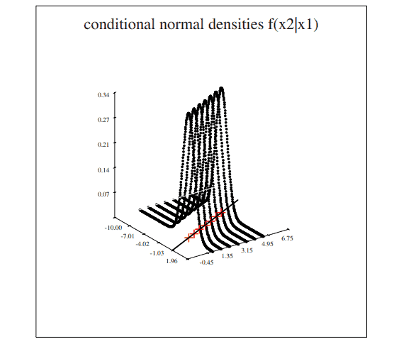
统计代写|多元统计分析代写Multivariate Statistical Analysis代考|Conditional Approximations
As we saw in Chapter 4 (Theorem 4.3), the conditional expectation $E\left(X_2 \mid X_1\right)$ is the mean squared error (MSE) best approximation of $X_2$ by a function of $X_1$. We have in this case that
$$
X_2=E\left(X_2 \mid X_1\right)+U=\mu_2+\Sigma_{21} \Sigma_{11}^{-1}\left(X_1-\mu_1\right)+U
$$
Hence, the best approximation of $X_2 \in \mathbb{R}^{p-r}$ by $X_1 \in \mathbb{R}^r$ is the linear approximation that can be written as:
$$
X_2=\beta_0+\mathcal{B} X_1+U
$$
with $\mathcal{B}=\Sigma_{21} \Sigma_{11}^{-1}, \beta_0=\mu_2-B \mu_1$ and $U \sim N\left(0, \Sigma_{22.1}\right)$.
Consider now the particular case where $r=p-1$. Now $X_2 \in \mathbb{R}$ and $\mathcal{B}$ is a row vector $\beta^{\top}$ of dimension $(1 \times r)$
$$
X_2=\beta_0+\beta^{\top} X_1+U
$$
This means, geometrically speaking, that the best MSE approximation of $X_2$ by a function of $X_1$ is hyperplane. The marginal variance of $X_2$ can be decomposed via (5.11):
$$
\sigma_{22}=\beta^{\top} \Sigma_{11} \beta+\sigma_{22.1}=\sigma_{21} \Sigma_{11}^{-1} \sigma_{12}+\sigma_{22.1} .
$$
The ratio
$$
\rho_{2.1 \ldots r}^2=\frac{\sigma_{21} \Sigma_{11}^{-1} \sigma_{12}}{\sigma_{22}}
$$
is known as the square of the multiple correlation between $X_2$ and the $r$ variables $X_1$. It is the percentage of the variance of $X_2$ which is explained by the linear approximation $\beta_0+\beta^{\top} X_1$. The last term in (5.12) is the residual variance of $X_2$. The square of the multiple correlation corresponds to the coefficient of determination introduced in Section 3.4, see (3.39), but here it is defined in terms of the r.v. $X_1$ and $X_2$. It can be shown that $\rho_{2.1 \ldots r}$ is also the maximum correlation attainable between $X_2$ and a linear combination of the elements of $X_1$, the optimal linear combination being precisely given by $\beta^{\top} X_1$. Note, that when $r=1$, the multiple correlation $\rho_{2.1}$ coincides with the usual simple correlation $\rho_{X_2 X_1}$ between $X_2$ and $X_1$.
多元统计分析代考
统计代写|多元统计分析代写Multivariate Statistical Analysis代考|Elementary Properties of the Multinormal
让我们先总结一下在前一章中已经推导出来的一些性质。
$X \sim N_p(\mu, \Sigma)$的pdf格式为
$$
f(x)=|2 \pi \Sigma|^{-1 / 2} \exp \left{-\frac{1}{2}(x-\mu)^{\top} \Sigma^{-1}(x-\mu)\right} .
$$
期望为$E(X)=\mu$,协方差可计算为$\operatorname{Var}(X)=$$E(X-\mu)(X-\mu)^{\top}=\Sigma$。
线性变换将正态随机变量转化为正态随机变量。如果$X \sim N_p(\mu, \Sigma)$和$\mathcal{A}(p \times p), c \in \mathbb{R}^p$,那么$Y=\mathcal{A} X+c$是$p$ -变量正态,即
$$
Y \sim N_p\left(\mathcal{A} \mu+c, \mathcal{A} \Sigma \mathcal{A}^{\top}\right)
$$
如果$X \sim N_p(\mu, \Sigma)$,那么马氏变换是
$$
Y=\Sigma^{-1 / 2}(X-\mu) \sim N_p\left(0, \mathcal{I}_p\right)
$$
它认为
$$
Y^{\top} Y=(X-\mu)^{\top} \Sigma^{-1}(X-\mu) \sim \chi_p^2
$$
通常将$X$划分为子向量$X_1$和$X_2$是很有趣的。下面的定理告诉我们如何修正$X_2$以得到一个与$X_1$无关的向量。
统计代写|多元统计分析代写Multivariate Statistical Analysis代考|Conditional Approximations
正如我们在第4章(定理4.3)中看到的,条件期望$E\left(X_2 \mid X_1\right)$是$X_1$的函数对$X_2$的均方误差(MSE)的最佳逼近。在这种情况下
$$
X_2=E\left(X_2 \mid X_1\right)+U=\mu_2+\Sigma_{21} \Sigma_{11}^{-1}\left(X_1-\mu_1\right)+U
$$
因此,$X_1 \in \mathbb{R}^r$对$X_2 \in \mathbb{R}^{p-r}$的最佳近似是线性近似,可以写成:
$$
X_2=\beta_0+\mathcal{B} X_1+U
$$
有$\mathcal{B}=\Sigma_{21} \Sigma_{11}^{-1}, \beta_0=\mu_2-B \mu_1$和$U \sim N\left(0, \Sigma_{22.1}\right)$。
现在考虑$r=p-1$。现在$X_2 \in \mathbb{R}$和$\mathcal{B}$是维数$(1 \times r)$的行向量$\beta^{\top}$
$$
X_2=\beta_0+\beta^{\top} X_1+U
$$
这意味着,从几何上讲,$X_1$的函数对$X_2$的最佳MSE近似是超平面。$X_2$的边际方差可由式(5.11)分解:
$$
\sigma_{22}=\beta^{\top} \Sigma_{11} \beta+\sigma_{22.1}=\sigma_{21} \Sigma_{11}^{-1} \sigma_{12}+\sigma_{22.1} .
$$
比率
$$
\rho_{2.1 \ldots r}^2=\frac{\sigma_{21} \Sigma_{11}^{-1} \sigma_{12}}{\sigma_{22}}
$$
称为$X_2$与$r$变量$X_1$之间的多重相关的平方。它是由线性近似$\beta_0+\beta^{\top} X_1$解释的$X_2$方差的百分比。(5.12)中的最后一项是$X_2$的残差方差。多重相关的平方对应于3.4节中引入的决定系数,参见(3.39),但在这里它是根据rv $X_1$和$X_2$定义的。可以证明,$\rho_{2.1 \ldots r}$也是$X_2$与$X_1$元素的线性组合之间可以达到的最大相关性,最优线性组合由$\beta^{\top} X_1$精确给出。请注意,当$r=1$时,多重相关性$\rho_{2.1}$与$X_2$和$X_1$之间通常的简单相关性$\rho_{X_2 X_1}$相吻合。

统计代写请认准statistics-lab™. statistics-lab™为您的留学生涯保驾护航。
金融工程代写
金融工程是使用数学技术来解决金融问题。金融工程使用计算机科学、统计学、经济学和应用数学领域的工具和知识来解决当前的金融问题,以及设计新的和创新的金融产品。
非参数统计代写
非参数统计指的是一种统计方法,其中不假设数据来自于由少数参数决定的规定模型;这种模型的例子包括正态分布模型和线性回归模型。
广义线性模型代考
广义线性模型(GLM)归属统计学领域,是一种应用灵活的线性回归模型。该模型允许因变量的偏差分布有除了正态分布之外的其它分布。
术语 广义线性模型(GLM)通常是指给定连续和/或分类预测因素的连续响应变量的常规线性回归模型。它包括多元线性回归,以及方差分析和方差分析(仅含固定效应)。
有限元方法代写
有限元方法(FEM)是一种流行的方法,用于数值解决工程和数学建模中出现的微分方程。典型的问题领域包括结构分析、传热、流体流动、质量运输和电磁势等传统领域。
有限元是一种通用的数值方法,用于解决两个或三个空间变量的偏微分方程(即一些边界值问题)。为了解决一个问题,有限元将一个大系统细分为更小、更简单的部分,称为有限元。这是通过在空间维度上的特定空间离散化来实现的,它是通过构建对象的网格来实现的:用于求解的数值域,它有有限数量的点。边界值问题的有限元方法表述最终导致一个代数方程组。该方法在域上对未知函数进行逼近。[1] 然后将模拟这些有限元的简单方程组合成一个更大的方程系统,以模拟整个问题。然后,有限元通过变化微积分使相关的误差函数最小化来逼近一个解决方案。
tatistics-lab作为专业的留学生服务机构,多年来已为美国、英国、加拿大、澳洲等留学热门地的学生提供专业的学术服务,包括但不限于Essay代写,Assignment代写,Dissertation代写,Report代写,小组作业代写,Proposal代写,Paper代写,Presentation代写,计算机作业代写,论文修改和润色,网课代做,exam代考等等。写作范围涵盖高中,本科,研究生等海外留学全阶段,辐射金融,经济学,会计学,审计学,管理学等全球99%专业科目。写作团队既有专业英语母语作者,也有海外名校硕博留学生,每位写作老师都拥有过硬的语言能力,专业的学科背景和学术写作经验。我们承诺100%原创,100%专业,100%准时,100%满意。
随机分析代写
随机微积分是数学的一个分支,对随机过程进行操作。它允许为随机过程的积分定义一个关于随机过程的一致的积分理论。这个领域是由日本数学家伊藤清在第二次世界大战期间创建并开始的。
时间序列分析代写
随机过程,是依赖于参数的一组随机变量的全体,参数通常是时间。 随机变量是随机现象的数量表现,其时间序列是一组按照时间发生先后顺序进行排列的数据点序列。通常一组时间序列的时间间隔为一恒定值(如1秒,5分钟,12小时,7天,1年),因此时间序列可以作为离散时间数据进行分析处理。研究时间序列数据的意义在于现实中,往往需要研究某个事物其随时间发展变化的规律。这就需要通过研究该事物过去发展的历史记录,以得到其自身发展的规律。
回归分析代写
多元回归分析渐进(Multiple Regression Analysis Asymptotics)属于计量经济学领域,主要是一种数学上的统计分析方法,可以分析复杂情况下各影响因素的数学关系,在自然科学、社会和经济学等多个领域内应用广泛。
MATLAB代写
MATLAB 是一种用于技术计算的高性能语言。它将计算、可视化和编程集成在一个易于使用的环境中,其中问题和解决方案以熟悉的数学符号表示。典型用途包括:数学和计算算法开发建模、仿真和原型制作数据分析、探索和可视化科学和工程图形应用程序开发,包括图形用户界面构建MATLAB 是一个交互式系统,其基本数据元素是一个不需要维度的数组。这使您可以解决许多技术计算问题,尤其是那些具有矩阵和向量公式的问题,而只需用 C 或 Fortran 等标量非交互式语言编写程序所需的时间的一小部分。MATLAB 名称代表矩阵实验室。MATLAB 最初的编写目的是提供对由 LINPACK 和 EISPACK 项目开发的矩阵软件的轻松访问,这两个项目共同代表了矩阵计算软件的最新技术。MATLAB 经过多年的发展,得到了许多用户的投入。在大学环境中,它是数学、工程和科学入门和高级课程的标准教学工具。在工业领域,MATLAB 是高效研究、开发和分析的首选工具。MATLAB 具有一系列称为工具箱的特定于应用程序的解决方案。对于大多数 MATLAB 用户来说非常重要,工具箱允许您学习和应用专业技术。工具箱是 MATLAB 函数(M 文件)的综合集合,可扩展 MATLAB 环境以解决特定类别的问题。可用工具箱的领域包括信号处理、控制系统、神经网络、模糊逻辑、小波、仿真等。