标签: STA321

统计代写|回归分析作业代写Regression Analysis代考|STA321

如果你也在 怎样代写回归分析Regression Analysis 这个学科遇到相关的难题,请随时右上角联系我们的24/7代写客服。回归分析Regression Analysis是一种显示两个或多个变量之间关系的统计方法。通常用图表表示,该方法检验因变量与自变量之间的关系。通常,自变量随因变量而变化,回归分析试图回答哪些因素对这种变化最重要。

回归分析Regression Analysis中的预测可以涵盖各种各样的情况和场景。例如,预测有多少人会看到广告牌可以帮助管理层决定投资广告是否是个好主意;在哪种情况下,这个广告牌能提供良好的投资回报?保险公司和银行大量使用回归分析的预测。有多少抵押贷款持有人会按时偿还贷款?有多少投保人会遭遇车祸或家中被盗?这些预测允许进行风险评估,但也可以预测最佳费用和溢价。

statistics-lab™ 为您的留学生涯保驾护航 在代写回归分析Regression Analysis方面已经树立了自己的口碑, 保证靠谱, 高质且原创的统计Statistics代写服务。我们的专家在代写回归分析Regression Analysis代写方面经验极为丰富,各种代写回归分析Regression Analysis相关的作业也就用不着说。

统计代写|回归分析作业代写Regression Analysis代考|STA321

统计代写|回归分析作业代写Regression Analysis代考|Piecewise Linear Regression; Regime Analysis

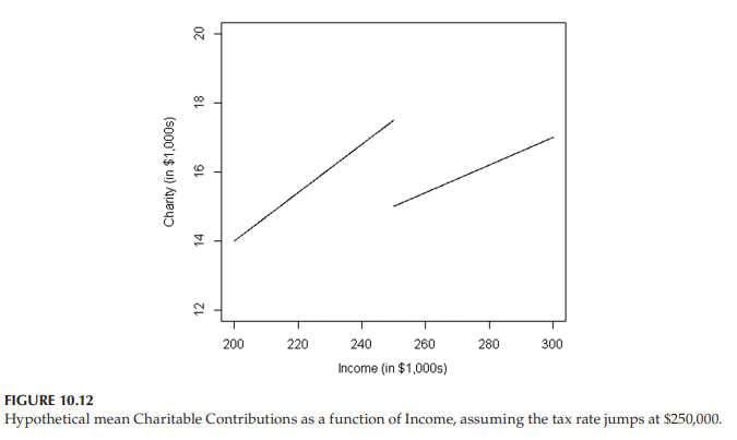
Usually, it makes sense to model $\mathrm{E}(Y \mid X=x)$ as a continuous function of $x$, but there are cases where a discontinuity is needed. For a hypothetical example, suppose people with less than $\$ 250,000$ income are taxed at $28 \%$, and those with $\$ 250,000$ or more are taxed at $34 \%$. Then a regression model to predict $Y=$ Charitable Contributions will likely have a discontinuity at $X=250,000$, as shown in Figure 10.12.

If you wanted to estimate the model shown in Figure 10.12, you would first create an indicator variable that is 0 for Income $<250$, otherwise 1 , like this:
Ind $=$ ifelse $($ Income $<250,0,1)$
Then you would include that variable in a regression model, with interactions, like this:
$$
\text { Charity }=\beta_0+\beta_1 \text { Income }+\beta_2 \text { Ind }+\beta_3 \text { Income } \times \text { Ind }+\varepsilon
$$
How can you understand this model? Once again, you must separate the model into the various subgroups. Here there are models in this example:
Group 1: Income $<250$
$$
\begin{aligned}
\text { Charity } & =\beta_0+\beta_1 \text { Income }+\beta_2(0)+\beta_3 \text { Income } \times(0)+\varepsilon \
& =\beta_0+\beta_1 \text { Income }+\varepsilon
\end{aligned}
$$
Group 2: Income $\geq 250$
$$
\begin{aligned}
\text { Charity } & =\beta_0+\beta_1 \text { Income }+\beta_2(1)+\beta_3 \text { Income } \times(1)+\varepsilon \
& =\left(\beta_0+\beta_2\right)+\left(\beta_1+\beta_3\right) \text { Income }+\varepsilon
\end{aligned}
$$
Thus, $\beta_0$ and $\beta_1$ are the intercept and slope of the model when Income $<250$, while $\left(\beta_0+\beta_2\right)$ and $\left(\beta_1+\beta_2\right)$ are the intercept and slope of the model when Income $\geq 250$.

统计代写|回归分析作业代写Regression Analysis代考|Relationship Between Commodity Price and Commodity Stockpile

The following data set contains government-reported annual numbers for price (Price) and stockpiles (Stocks) of a particular agricultural commodity in an Asian country.
Comm = read.table (“https://raw.githubusercontent.com/andrea2719/
URA-DataSets/master/Comm_Price.txt”)
attach(Comm)
Comm = read.table $($ https $: / /$ raw.githubusercontent. com/andrea $2719 /$
URA-DataSets/master/Comm_Price.txt”)
attach (Comm)
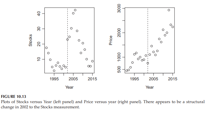
Figure 10.13 shows how the Stocks and Price have changed over time. Something happened in 2002 to the Stocks variable; perhaps a re-definition of the measurement in response to a policy change.

This abrupt shift in 2002 causes trouble in estimating the relationship between Price and Stocks, which would ordinarily be considered a negative one because of the laws of supply and demand. Figure 10.14 shows the (Stocks, Price) scatter, with data values before 2002 indicated by circles, as well as global and separate least-squares fits.

$\mathrm{R}$ code for Figure 10.14
pch = ifelse $($ Year $<2002,1,2)$ par (mfrow=c $(1,2))$ plot (Stocks, Price, pch=pch) abline (lsfit (Stocks, Price)) plot (Stocks, Price, pch=pch) abline (lsfit (Stocks [Year $<2002$ ], Price [Year<2002]), 1ty=1) abline (Isfit (Stocks [Year $>=2002$ ], Price [Year $>=2002$ ]), Ity=2)

统计代写|回归分析作业代写Regression Analysis代考|STA321

回归分析代写

统计代写|回归分析作业代写Regression Analysis代考|Piecewise Linear Regression; Regime Analysis

通常,将$\mathrm{E}(Y \mid X=x)$建模为$x$的连续函数是有意义的,但也有需要不连续的情况。举个假设的例子,假设收入低于$\$ 250,000$的人按$28 \%$征税,收入高于$\$ 250,000$的人按$34 \%$征税。然后,回归模型预测$Y=$慈善捐款可能在$X=250,000$处具有不连续,如图10.12所示。

如果你想估计如图10.12所示的模型,你首先要为Income $<250$创建一个0的指标变量,否则为1,如下所示:
Ind $=$如果没有$($收入$<250,0,1)$
然后将该变量包含在回归模型中,并进行交互,如下所示:
$$
\text { Charity }=\beta_0+\beta_1 \text { Income }+\beta_2 \text { Ind }+\beta_3 \text { Income } \times \text { Ind }+\varepsilon
$$
你如何理解这个模型?同样,您必须将模型分成不同的子组。在这个例子中有一些模型:
第一组:收入$<250$
$$
\begin{aligned}
\text { Charity } & =\beta_0+\beta_1 \text { Income }+\beta_2(0)+\beta_3 \text { Income } \times(0)+\varepsilon \
& =\beta_0+\beta_1 \text { Income }+\varepsilon
\end{aligned}
$$
第二组:收入$\geq 250$
$$
\begin{aligned}
\text { Charity } & =\beta_0+\beta_1 \text { Income }+\beta_2(1)+\beta_3 \text { Income } \times(1)+\varepsilon \
& =\left(\beta_0+\beta_2\right)+\left(\beta_1+\beta_3\right) \text { Income }+\varepsilon
\end{aligned}
$$
因此,$\beta_0$和$\beta_1$为Income $<250$时模型的截距和斜率,$\left(\beta_0+\beta_2\right)$和$\left(\beta_1+\beta_2\right)$为Income $\geq 250$时模型的截距和斜率。

统计代写|回归分析作业代写Regression Analysis代考|Relationship Between Commodity Price and Commodity Stockpile

以下数据集包含政府报告的亚洲国家特定农产品价格(price)和库存(Stocks)的年度数字。
Comm = read。表(https://raw.githubusercontent.com/andrea2719/)
“URA-DataSets/master/Comm_Price.txt”)
随员(通讯)
Comm = read。表$($ HTTPS $: / /$ raw.githubusercontent。com andrea $2719 /$
“URA-DataSets/master/Comm_Price.txt”)
随员(通讯)
图10.13显示了股票和价格随时间的变化情况。2002年股票变量发生了变化;也许是为了响应政策变化而重新定义度量。

2002年的这种突然转变给估计价格和股票之间的关系带来了麻烦,由于供求规律,这种关系通常被认为是负相关的。图10.14显示了(股票,价格)散点,2002年之前的数据值用圆圈表示,以及全局和单独的最小二乘拟合。

$\mathrm{R}$ 代码见图10.14
pch= ifelse $($ Year $<2002,1,2)$ par (mfrow=c $(1,2))$ plot (Stocks, Price, pch=pch) abline (lsfit (Stocks, Price)) plot (Stocks, Price, pch=pch) abline (lsfit (Stocks [Year $<2002$], Price [Year<2002]), 1ty=1) abline (Isfit (Stocks [Year $>=2002$], Price [Year $>=2002$]), Ity=2)

统计代写|回归分析作业代写Regression Analysis代考 请认准statistics-lab™

统计代写请认准statistics-lab™. statistics-lab™为您的留学生涯保驾护航。

微观经济学代写

微观经济学是主流经济学的一个分支,研究个人和企业在做出有关稀缺资源分配的决策时的行为以及这些个人和企业之间的相互作用。my-assignmentexpert™ 为您的留学生涯保驾护航 在数学Mathematics作业代写方面已经树立了自己的口碑, 保证靠谱, 高质且原创的数学Mathematics代写服务。我们的专家在图论代写Graph Theory代写方面经验极为丰富,各种图论代写Graph Theory相关的作业也就用不着 说。

线性代数代写

线性代数是数学的一个分支,涉及线性方程,如:线性图,如:以及它们在向量空间和通过矩阵的表示。线性代数是几乎所有数学领域的核心。

博弈论代写

现代博弈论始于约翰-冯-诺伊曼(John von Neumann)提出的两人零和博弈中的混合策略均衡的观点及其证明。冯-诺依曼的原始证明使用了关于连续映射到紧凑凸集的布劳威尔定点定理,这成为博弈论和数学经济学的标准方法。在他的论文之后,1944年,他与奥斯卡-莫根斯特恩(Oskar Morgenstern)共同撰写了《游戏和经济行为理论》一书,该书考虑了几个参与者的合作游戏。这本书的第二版提供了预期效用的公理理论,使数理统计学家和经济学家能够处理不确定性下的决策。

微积分代写

微积分,最初被称为无穷小微积分或 “无穷小的微积分”,是对连续变化的数学研究,就像几何学是对形状的研究,而代数是对算术运算的概括研究一样。

它有两个主要分支,微分和积分;微分涉及瞬时变化率和曲线的斜率,而积分涉及数量的累积,以及曲线下或曲线之间的面积。这两个分支通过微积分的基本定理相互联系,它们利用了无限序列和无限级数收敛到一个明确定义的极限的基本概念 。

计量经济学代写

什么是计量经济学?
计量经济学是统计学和数学模型的定量应用,使用数据来发展理论或测试经济学中的现有假设,并根据历史数据预测未来趋势。它对现实世界的数据进行统计试验,然后将结果与被测试的理论进行比较和对比。

根据你是对测试现有理论感兴趣,还是对利用现有数据在这些观察的基础上提出新的假设感兴趣,计量经济学可以细分为两大类:理论和应用。那些经常从事这种实践的人通常被称为计量经济学家。

Matlab代写

MATLAB 是一种用于技术计算的高性能语言。它将计算、可视化和编程集成在一个易于使用的环境中,其中问题和解决方案以熟悉的数学符号表示。典型用途包括:数学和计算算法开发建模、仿真和原型制作数据分析、探索和可视化科学和工程图形应用程序开发,包括图形用户界面构建MATLAB 是一个交互式系统,其基本数据元素是一个不需要维度的数组。这使您可以解决许多技术计算问题,尤其是那些具有矩阵和向量公式的问题,而只需用 C 或 Fortran 等标量非交互式语言编写程序所需的时间的一小部分。MATLAB 名称代表矩阵实验室。MATLAB 最初的编写目的是提供对由 LINPACK 和 EISPACK 项目开发的矩阵软件的轻松访问,这两个项目共同代表了矩阵计算软件的最新技术。MATLAB 经过多年的发展,得到了许多用户的投入。在大学环境中,它是数学、工程和科学入门和高级课程的标准教学工具。在工业领域,MATLAB 是高效研究、开发和分析的首选工具。MATLAB 具有一系列称为工具箱的特定于应用程序的解决方案。对于大多数 MATLAB 用户来说非常重要,工具箱允许您学习应用专业技术。工具箱是 MATLAB 函数(M 文件)的综合集合,可扩展 MATLAB 环境以解决特定类别的问题。可用工具箱的领域包括信号处理、控制系统、神经网络、模糊逻辑、小波、仿真等。

R语言代写问卷设计与分析代写
PYTHON代写回归分析与线性模型代写
MATLAB代写方差分析与试验设计代写
STATA代写机器学习/统计学习代写
SPSS代写计量经济学代写
EVIEWS代写时间序列分析代写
EXCEL代写深度学习代写
SQL代写各种数据建模与可视化代写

统计代写|回归分析作业代写Regression Analysis代考|ST430

如果你也在 怎样代写回归分析Regression Analysis 这个学科遇到相关的难题,请随时右上角联系我们的24/7代写客服。回归分析Regression Analysis是一种显示两个或多个变量之间关系的统计方法。通常用图表表示,该方法检验因变量与自变量之间的关系。通常,自变量随因变量而变化,回归分析试图回答哪些因素对这种变化最重要。

回归分析Regression Analysis中的预测可以涵盖各种各样的情况和场景。例如,预测有多少人会看到广告牌可以帮助管理层决定投资广告是否是个好主意;在哪种情况下,这个广告牌能提供良好的投资回报?保险公司和银行大量使用回归分析的预测。有多少抵押贷款持有人会按时偿还贷款?有多少投保人会遭遇车祸或家中被盗?这些预测允许进行风险评估,但也可以预测最佳费用和溢价。

statistics-lab™ 为您的留学生涯保驾护航 在代写回归分析Regression Analysis方面已经树立了自己的口碑, 保证靠谱, 高质且原创的统计Statistics代写服务。我们的专家在代写回归分析Regression Analysis代写方面经验极为丰富,各种代写回归分析Regression Analysis相关的作业也就用不着说。

统计代写|回归分析作业代写Regression Analysis代考|ST430

统计代写|回归分析作业代写Regression Analysis代考|Does Location Affect House Price, Controlling for House Size?

Even though the realtors say “location, location, location!”, the observed effects of location on house price might simply be due to the fact that bigger homes tend to be in some locations. After all, square footage is a strong determinant of house price. To compare prices in different locations for homes of the same size, simply add “sqfeet” to the model like this:
house = read.csv(“https://raw.githubusercontent.com/andrea2719/
URA-DataSets/master/house.csv”, header=T)
attach(house)
fit.main = lm(sell $~$ location + sqfeet, data=house)
summary (fit.main)
house $=$ read.csv $($ https: $/ /$ raw.githubusercontent.com/andrea $2719 /$
URA-Datasets/master/house.csv”, header=T)
attach (house)
fit.main $=1 \mathrm{~m}($ sell $\sim$ location + sqfeet, data=house)
summary (fit.main)
The results are as follows:
Coefficients :
Estimate std. Error $t$ value $\operatorname{Pr}(>|t|)$
$\begin{array}{lllll}\text { (Intercept) } 25.898669 & 5.060777 \quad 5.118 \quad 3.67 \mathrm{e}-06 * * *\end{array}$
locationB $-21.106407 \quad 2.152655-9.8056 .41 \mathrm{e}-14 * \star *$
locationd $-21.431288 \quad 3.579304 \quad-5.988 \quad 1.43 e-07 \star \star * *$
locationd $-24.846429 \quad 2.574269 \quad-9.6521 .13 \mathrm{e}-13 \star \star *$
locatione $-27.304759 \quad 2.538505-10.7561 .94 \mathrm{e}-15 * k *$
sqfeet $\quad 0.0412240 .002578 \quad 15.993<2 e-16 * k $ Signif. Codes: 0 ‘‘ 0.001 ‘‘ 0.01 ‘*’ $0.05 ‘ y^{\prime} 0.1$ ‘ 1
Residual standard error: 6.638 on 58 degrees of freedom
Multiple R-squared: 0.874, Adjusted R-squared: 0.8631
F-statistic: 80.47 on 5 and 58 DF, p-value: $<2.2 e-16$

统计代写|回归分析作业代写Regression Analysis代考|Full Model versus Restricted Model $F$ Tests

As we have mentioned repeatedly, tests of hypotheses are not the best way to evaluate models and assumptions. However, the $F$ test that was introduced in Chapter 8 is so common in the history of ANOVA, ANCOVA, and regression that we would be remiss not to mention it.

Models such as those shown in Figures 10.7 and 10.6 are often compared by using the $F$ test, which is a test to compare “full” versus “restricted” classical regression models. (For models other than the classical regression model, full/restricted model comparison is more commonly done using the likelihood ratio test, which is used starting in Chapter 12 of this book.)
In the usual regression analysis, a full model typically has the form:
$$
Y=\beta_0+\beta_1 X_1+\beta_2 X_2+\ldots+\beta_k X_k+\varepsilon
$$
Here, the parameters $\beta_0, \beta_1, \beta_2, \ldots$, and $\beta_k$ are unconstrained; that is, each parameter can possibly take any value whatsoever between $-\infty$ and $\infty$, and the value that one $\beta$ parameter takes is not dependent on (or constrained by) the value that any other $\beta$ parameter takes.
A restricted model is the same model, but with constraints on the parameters. The most common restrictions are constraints such as $\beta_1=\beta_2=0$, although other constraints such as $\beta_2=1$, or $\beta_1-\beta_2=0$, or $\beta_0+15 \beta_2=100$ are also possible.

The separate slope model graphed in Figure 10.7 is a full model relative to the restricted model that constrains all the interaction $\beta^{\prime}$ s to be zero, shown in Figure 10.6. The $F$ test can be used to compare these models. To construct the $F$ test, let $\mathrm{SSE}{\mathrm{F}}$ denote the error sum of squares in the full model, and let $\mathrm{SSE}{\mathrm{R}}$ denote the error sum of squares in the restricted model. It is a mathematical fact that
$$
\mathrm{SSE}{\mathrm{F}} \leq \mathrm{SSE}{\mathrm{R}}
$$

统计代写|回归分析作业代写Regression Analysis代考|ST430

回归分析代写

统计代写|回归分析作业代写Regression Analysis代考|Does Location Affect House Price, Controlling for House Size?

尽管房地产经纪人说“地段,地段,地段!”,但所观察到的地段对房价的影响可能仅仅是因为某些地段往往有更大的房子。毕竟,面积是房价的重要决定因素。要比较相同面积的房屋在不同地点的价格,只需在模型中添加“平方英尺”,如下所示:
House = read.csv(“https://raw.githubusercontent.com/andrea2719/ .csv “)
“URA-DataSets/master/house.csv”,header=T)
附属(屋宇)
适合。Main = lm(sell $~$ location + sqfeet, data=house)
摘要(fit.main)
House $=$ read.csv $($ https: $/ /$ raw.githubusercontent.com/andrea $2719 /$
“URA-Datasets/master/house.csv”,header=T)
随员(屋宇)
适合。主$=1 \mathrm{~m}($出售$\sim$位置+平方英尺,数据=房子)
摘要(fit.main)
结果如下:
系数:
估计std误差$t$值$\operatorname{Pr}(>|t|)$
$\begin{array}{lllll}\text { (Intercept) } 25.898669 & 5.060777 \quad 5.118 \quad 3.67 \mathrm{e}-06 * * *\end{array}$
locationB $-21.106407 \quad 2.152655-9.8056 .41 \mathrm{e}-14 * \star *$
位置$-21.431288 \quad 3.579304 \quad-5.988 \quad 1.43 e-07 \star \star * *$
位置$-24.846429 \quad 2.574269 \quad-9.6521 .13 \mathrm{e}-13 \star \star *$
位置$-27.304759 \quad 2.538505-10.7561 .94 \mathrm{e}-15 * k *$
sqfeet $\quad 0.0412240 .002578 \quad 15.993<2 e-16 * k $标志。代码:0“0.001”0.01“*”$0.05 ‘ y^{\prime} 0.1$
残差标准误差:6.638在58个自由度
多元r平方:0.874,调整r平方:0.8631
f统计量在5和58 DF上为80.47,p值: $<2.2 e-16$

统计代写|回归分析作业代写Regression Analysis代考|Full Model versus Restricted Model $F$ Tests

正如我们反复提到的,假设检验并不是评估模型和假设的最佳方式。然而,在第8章中介绍的$F$测试在ANOVA, ANCOVA和回归的历史中是如此常见,以至于我们将忽略它。

图10.7和10.6中所示的模型通常使用$F$测试进行比较,这是一个比较“完整”和“受限”经典回归模型的测试。(对于经典回归模型以外的模型,完整/受限模型比较更常用的方法是使用似然比检验,从本书第12章开始使用。)
在通常的回归分析中,一个完整的模型通常有这样的形式:
$$
Y=\beta_0+\beta_1 X_1+\beta_2 X_2+\ldots+\beta_k X_k+\varepsilon
$$
这里,参数$\beta_0, \beta_1, \beta_2, \ldots$和$\beta_k$是不受约束的;也就是说,每个参数可以取$-\infty$和$\infty$之间的任何值,并且一个$\beta$参数取的值不依赖于(或受限于)任何其他$\beta$参数取的值。
受限模型是相同的模型,但对参数有约束。最常见的限制是诸如$\beta_1=\beta_2=0$之类的约束,尽管其他约束如$\beta_2=1$、$\beta_1-\beta_2=0$或$\beta_0+15 \beta_2=100$也是可能的。

图10.7所示的独立斜率模型是相对于约束所有相互作用$\beta^{\prime}$ s为零的受限模型的完整模型,如图10.6所示。$F$测试可以用来比较这些模型。为了构造$F$检验,让$\mathrm{SSE}{\mathrm{F}}$表示完整模型中的误差平方和,让$\mathrm{SSE}{\mathrm{R}}$表示受限模型中的误差平方和。这是一个数学事实
$$
\mathrm{SSE}{\mathrm{F}} \leq \mathrm{SSE}{\mathrm{R}}
$$

统计代写|回归分析作业代写Regression Analysis代考 请认准statistics-lab™

统计代写请认准statistics-lab™. statistics-lab™为您的留学生涯保驾护航。

微观经济学代写

微观经济学是主流经济学的一个分支,研究个人和企业在做出有关稀缺资源分配的决策时的行为以及这些个人和企业之间的相互作用。my-assignmentexpert™ 为您的留学生涯保驾护航 在数学Mathematics作业代写方面已经树立了自己的口碑, 保证靠谱, 高质且原创的数学Mathematics代写服务。我们的专家在图论代写Graph Theory代写方面经验极为丰富,各种图论代写Graph Theory相关的作业也就用不着 说。

线性代数代写

线性代数是数学的一个分支,涉及线性方程,如:线性图,如:以及它们在向量空间和通过矩阵的表示。线性代数是几乎所有数学领域的核心。

博弈论代写

现代博弈论始于约翰-冯-诺伊曼(John von Neumann)提出的两人零和博弈中的混合策略均衡的观点及其证明。冯-诺依曼的原始证明使用了关于连续映射到紧凑凸集的布劳威尔定点定理,这成为博弈论和数学经济学的标准方法。在他的论文之后,1944年,他与奥斯卡-莫根斯特恩(Oskar Morgenstern)共同撰写了《游戏和经济行为理论》一书,该书考虑了几个参与者的合作游戏。这本书的第二版提供了预期效用的公理理论,使数理统计学家和经济学家能够处理不确定性下的决策。

微积分代写

微积分,最初被称为无穷小微积分或 “无穷小的微积分”,是对连续变化的数学研究,就像几何学是对形状的研究,而代数是对算术运算的概括研究一样。

它有两个主要分支,微分和积分;微分涉及瞬时变化率和曲线的斜率,而积分涉及数量的累积,以及曲线下或曲线之间的面积。这两个分支通过微积分的基本定理相互联系,它们利用了无限序列和无限级数收敛到一个明确定义的极限的基本概念 。

计量经济学代写

什么是计量经济学?
计量经济学是统计学和数学模型的定量应用,使用数据来发展理论或测试经济学中的现有假设,并根据历史数据预测未来趋势。它对现实世界的数据进行统计试验,然后将结果与被测试的理论进行比较和对比。

根据你是对测试现有理论感兴趣,还是对利用现有数据在这些观察的基础上提出新的假设感兴趣,计量经济学可以细分为两大类:理论和应用。那些经常从事这种实践的人通常被称为计量经济学家。

Matlab代写

MATLAB 是一种用于技术计算的高性能语言。它将计算、可视化和编程集成在一个易于使用的环境中,其中问题和解决方案以熟悉的数学符号表示。典型用途包括:数学和计算算法开发建模、仿真和原型制作数据分析、探索和可视化科学和工程图形应用程序开发,包括图形用户界面构建MATLAB 是一个交互式系统,其基本数据元素是一个不需要维度的数组。这使您可以解决许多技术计算问题,尤其是那些具有矩阵和向量公式的问题,而只需用 C 或 Fortran 等标量非交互式语言编写程序所需的时间的一小部分。MATLAB 名称代表矩阵实验室。MATLAB 最初的编写目的是提供对由 LINPACK 和 EISPACK 项目开发的矩阵软件的轻松访问,这两个项目共同代表了矩阵计算软件的最新技术。MATLAB 经过多年的发展,得到了许多用户的投入。在大学环境中,它是数学、工程和科学入门和高级课程的标准教学工具。在工业领域,MATLAB 是高效研究、开发和分析的首选工具。MATLAB 具有一系列称为工具箱的特定于应用程序的解决方案。对于大多数 MATLAB 用户来说非常重要,工具箱允许您学习应用专业技术。工具箱是 MATLAB 函数(M 文件)的综合集合,可扩展 MATLAB 环境以解决特定类别的问题。可用工具箱的领域包括信号处理、控制系统、神经网络、模糊逻辑、小波、仿真等。

R语言代写问卷设计与分析代写
PYTHON代写回归分析与线性模型代写
MATLAB代写方差分析与试验设计代写
STATA代写机器学习/统计学习代写
SPSS代写计量经济学代写
EVIEWS代写时间序列分析代写
EXCEL代写深度学习代写
SQL代写各种数据建模与可视化代写

统计代写|STAT311 Regression Analysis

Statistics-lab™可以为您提供metrostate.edu STAT311 Regression Analysis回归分析的代写代考辅导服务!

STAT311 Regression Analysis课程简介

This graduate level course offers an introduction into regression analysis. A
Credits 3 researcher is often interested in using sample data to investigate relationships, with an ultimate goal of creating a model to predict a future value for some dependent variable. The process of finding this mathematical model that best fits the data involves regression analysis.
STAT 501 is an applied linear regression course that emphasizes data analysis and interpretation. Generally, statistical regression is collection of methods for determining and using models that explain how a response variable (dependent variable) relates to one or more explanatory variables (predictor variables).

PREREQUISITES 

This graduate level course covers the following topics:

  • Understanding the context for simple linear regression.
  • How to evaluate simple linear regression models
  • How a simple linear regression model is used to estimate and predict likely values
  • Understanding the assumptions that need to be met for a simple linear regression model to be valid
  • How multiple predictors can be included into a regression model
  • Understanding the assumptions that need to be met when multiple predictors are included in the regression model for the model to be valid
  • How a multiple linear regression model is used to estimate and predict likely values
  • Understanding how categorical predictors can be included into a regression model
  • How to transform data in order to deal with problems identified in the regression model
  • Strategies for building regression models
  • Distinguishing between outliers and influential data points and how to deal with these
  • Handling problems typically encountered in regression contexts
  • Alternative methods for estimating a regression line besides using ordinary least squares
  • Understanding regression models in time dependent contexts
  • Understanding regression models in non-linear contexts

STAT311 Regression Analysis HELP(EXAM HELP, ONLINE TUTOR)

问题 1.

Use the cig_1st_diff data set. This is based on the changes from 1990 to 2000 , and it is extracted from the data set used in Question #3. Estimate a first-difference model, as follows: regress cigch on taxch, uratech, and beertaxch. Weight the model by pop 2000 , and use robust standard errors. Interpret the estimate on taxch.

问题 2.

From the example in Section 8.5 from Card and Krueger (1994) on estimating the effects of minimum-wage increases on employment, write out the regression equation for the difference-in-difference model.

问题 3.

Use the data set oecd_gas_demand. From Question #7 in Chapter 3, add fixed effects for the country, along with a heteroskedasticity correction.
a. How does the coefficient estimate on lrpmg change from Question #7 in Chapter 3 with the fixed effects added?
b. How does this change which observations are compared to which observations?

问题 4.

Return to the tv-bmi-ecls data set used for Exercise $# 5$ in Chapter 6 . From that exercise, along with other descriptions of the research issue, there is much potential omitted-factors bias.
a. Explore the data description and variable list (from the file “Exercises data set descriptions” on the book’s website). Design a model to address the omitted-factors bias.
b. Are there any shortcomings to your approach?

Textbooks


• An Introduction to Stochastic Modeling, Fourth Edition by Pinsky and Karlin (freely
available through the university library here)
• Essentials of Stochastic Processes, Third Edition by Durrett (freely available through
the university library here)
To reiterate, the textbooks are freely available through the university library. Note that
you must be connected to the university Wi-Fi or VPN to access the ebooks from the library
links. Furthermore, the library links take some time to populate, so do not be alarmed if
the webpage looks bare for a few seconds.

此图像的alt属性为空;文件名为%E7%B2%89%E7%AC%94%E5%AD%97%E6%B5%B7%E6%8A%A5-1024x575-10.png
统计代写|STAT311 Regression Analysis

Statistics-lab™可以为您提供metrostate.edu STAT311 Regression Analysis回归分析的代写代考辅导服务! 请认准Statistics-lab™. Statistics-lab™为您的留学生涯保驾护航。

统计代写|STAT501 Regression Analysis

Statistics-lab™可以为您提供metrostate.edu STAT501 Regression Analysis回归分析的代写代考辅导服务!

STAT501 Regression Analysis课程简介

This graduate level course offers an introduction into regression analysis. A
Credits 3 researcher is often interested in using sample data to investigate relationships, with an ultimate goal of creating a model to predict a future value for some dependent variable. The process of finding this mathematical model that best fits the data involves regression analysis.
STAT 501 is an applied linear regression course that emphasizes data analysis and interpretation. Generally, statistical regression is collection of methods for determining and using models that explain how a response variable (dependent variable) relates to one or more explanatory variables (predictor variables).

PREREQUISITES 

This graduate level course covers the following topics:

  • Understanding the context for simple linear regression.
  • How to evaluate simple linear regression models
  • How a simple linear regression model is used to estimate and predict likely values
  • Understanding the assumptions that need to be met for a simple linear regression model to be valid
  • How multiple predictors can be included into a regression model
  • Understanding the assumptions that need to be met when multiple predictors are included in the regression model for the model to be valid
  • How a multiple linear regression model is used to estimate and predict likely values
  • Understanding how categorical predictors can be included into a regression model
  • How to transform data in order to deal with problems identified in the regression model
  • Strategies for building regression models
  • Distinguishing between outliers and influential data points and how to deal with these
  • Handling problems typically encountered in regression contexts
  • Alternative methods for estimating a regression line besides using ordinary least squares
  • Understanding regression models in time dependent contexts
  • Understanding regression models in non-linear contexts

STAT501 Regression Analysis HELP(EXAM HELP, ONLINE TUTOR)

问题 1.

  1. Indicate which of the four main regression objectives each of the following research issues would be:
    a. What 4th-grade teacher did best given his/her students’ prior achievement?
    b. What is the best guess for how many sailors the Navy will recruit this year?
    c. Do people who swear have higher intelligence?
    d. How much does keeping up with the material affect your eventual grade in the class?
    e. Does keeping up with the material affect your eventual grade in the class?

问题 2.

  1. Suppose that, in a particular city, a regression of prices of homes sold in the prior year (price) on the number of bedrooms (bedrooms) and square feet (sqft) yields the following regression model:
    $$
    \widehat{\text { price }}=100,000+45,000 \times \text { bedrooms }+10 \times \text { sqft }
    $$
    a. Interpret the coefficient estimate on sqfi.
    b. If a home had 2 bedrooms and was 1500 square feet, what would the predicted price be?
    c. If that home had a selling price of $\$ 170,000$, what would be the residual?
    d. How would you interpret the residual?
    e. What is a possible reason for the residual being what it is?

问题 3.

3. From the book’s website, use the data set, democracy2. This is a data set of observations by country and year, with measures of democracy, life expectancy, and several other factors and outcomes. (see https://www.v-dem.net/). Use 1985 observations with condition1=1 (which is that there are non-missing values for all variables used in this regression).
a. Calculate the means and standard deviations of the following four variables to get a sense of the scales of the variable:

  • life_exp (life expectancy)
  • democracy (an index of the level of democracy in a county on a 0-1 scale)
  • augeduc (average years of education)
  • educgini (inequality Gini coefficient for years of education, on a 0-100 scale).
    b. Regress life_exp on democracy, avgeduc, and educgini. Interpret the coefficient estimate on democracy.
    c. For a country with life-exp $=60$, democracy $=0.5$, avgeduc $=10$, and educgini $=50$, what is the predicted value of the dependent variable and the residual?
    d. Interpret the predicted value and the residual.
    e. Interpret the $R^2$.
    f. Add urbanpct (the percent of the population living in an urban area) as an explanatory variable to the model. Interpret the change in $R^2$ after adding urbanpct.

问题 4.

4. From the book’s website, use the data set, income. Estimate three separate models, with income as the dependent variable. Include just one of the three explanatory variables (educ, afqt, age) in each model. Which explanatory variable explains the greatest amount of variation in income? How did you arrive at your answer?

Textbooks


• An Introduction to Stochastic Modeling, Fourth Edition by Pinsky and Karlin (freely
available through the university library here)
• Essentials of Stochastic Processes, Third Edition by Durrett (freely available through
the university library here)
To reiterate, the textbooks are freely available through the university library. Note that
you must be connected to the university Wi-Fi or VPN to access the ebooks from the library
links. Furthermore, the library links take some time to populate, so do not be alarmed if
the webpage looks bare for a few seconds.

此图像的alt属性为空;文件名为%E7%B2%89%E7%AC%94%E5%AD%97%E6%B5%B7%E6%8A%A5-1024x575-10.png
统计代写|STAT501 Regression Analysis

Statistics-lab™可以为您提供metrostate.edu STAT501 Regression Analysis回归分析的代写代考辅导服务! 请认准Statistics-lab™. Statistics-lab™为您的留学生涯保驾护航。