统计代写|线性回归代写linear regression代考|MATH5386
如果你也在 怎样代写线性回归linear regression这个学科遇到相关的难题,请随时右上角联系我们的24/7代写客服。
线性回归是对标量响应和一个或多个解释变量(也称为因变量和自变量)之间的关系进行建模的一种线性方法。一个解释变量的情况被称为简单线性回归。
statistics-lab™ 为您的留学生涯保驾护航 在代写线性回归linear regression方面已经树立了自己的口碑, 保证靠谱, 高质且原创的统计Statistics代写服务。我们的专家在代写线性回归linear regression代写方面经验极为丰富,各种代写线性回归linear regression相关的作业也就用不着说。
我们提供的线性回归linear regression及其相关学科的代写,服务范围广, 其中包括但不限于:
- Statistical Inference 统计推断
- Statistical Computing 统计计算
- Advanced Probability Theory 高等概率论
- Advanced Mathematical Statistics 高等数理统计学
- (Generalized) Linear Models 广义线性模型
- Statistical Machine Learning 统计机器学习
- Longitudinal Data Analysis 纵向数据分析
- Foundations of Data Science 数据科学基础
统计代写|线性回归代写linear regression代考|Checking Goodness of Fit
It is crucial to realize that an MLR model is not necessarily a useful model for the data, even if the data set consists of a response variable and several predictor variables. For example, a nonlinear regression model or a much more complicated model may be needed. Chapters 1 and 13 describe several alternative models. Let $p$ be the number of predictors and $n$ the number of cases. Assume that $n \geq 5 p$, then plots can be used to check whether the MLR model is useful for studying the data. This technique is known as checking the goodness of fit of the MLR model.
Notation. Plots will be used to simplify regression analysis, and in this text a plot of $W$ versus $Z$ uses $W$ on the horizontal axis and $Z$ on the vertical axis.
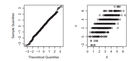
Definition 2.10. A scatterplot of $X$ versus $Y$ is a plot of $X$ versus $Y$ and is used to visualize the conditional distribution $Y \mid X$ of $Y$ given $X$.
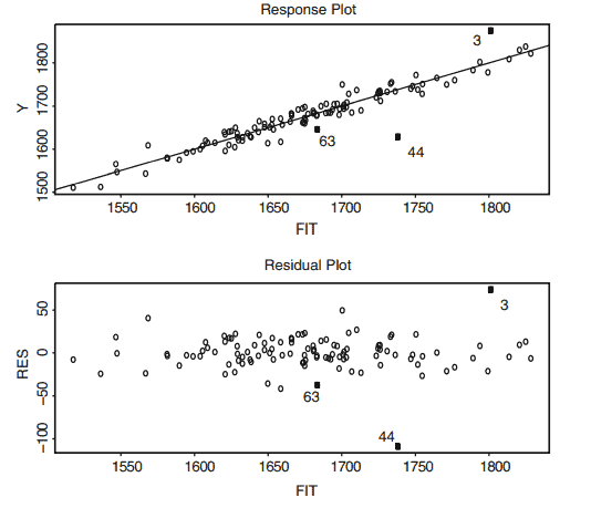
Definition 2.11. A response plot is a plot of a variable $w_i$ versus $Y_i$. Typically $w_i$ is a linear combination of the predictors: $w_i=\boldsymbol{x}_i^T \boldsymbol{\eta}$ where $\boldsymbol{\eta}$ is a known $p \times 1$ vector. The most commonly used response plot is a plot of the fitted values $\widehat{Y}_i$ versus the response $Y_i$.
Proposition 2.1. Suppose that the regression estimator $\boldsymbol{b}$ of $\boldsymbol{\beta}$ is used to find the residuals $r_i \equiv r_i(\boldsymbol{b})$ and the fitted values $\widehat{Y}_i \equiv \widehat{Y}_i(\boldsymbol{b})=\boldsymbol{x}_i^T \boldsymbol{b}$. Then in the response plot of $\widehat{Y}_i$ versus $Y_i$, the vertical deviations from the identity line (that has unit slope and zero intercept) are the residuals $r_i(b)$.
Proof. The identity line in the response plot is $Y=\boldsymbol{x}^T \boldsymbol{b}$. Hence the vertical deviation is $Y_i-\boldsymbol{x}_i^T \boldsymbol{b}=r_i(\boldsymbol{b})$.
Definition 2.12. A residual plot is a plot of a variable $w_i$ versus the residuals $r_i$. The most commonly used residual plot is a plot of $\hat{Y}_i$ versus $r_i$.
Notation: For MLR, “the residual plot” will often mean the residual plot of $\hat{Y}_i$ versus $r_i$, and “the response plot” will often mean the plot of $\hat{Y}_i$ versus $Y_i^*$
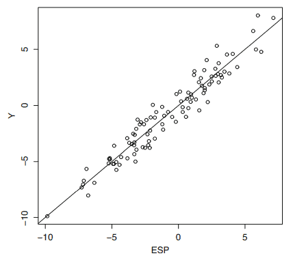
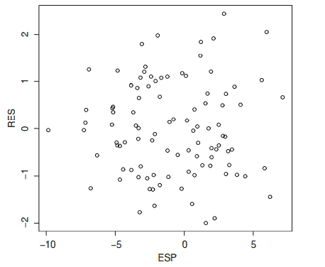
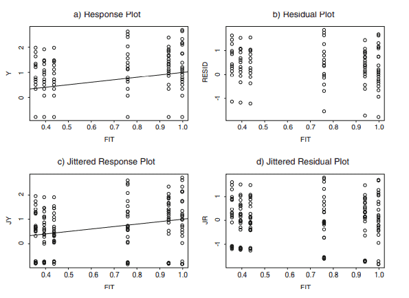
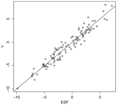
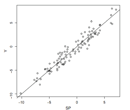
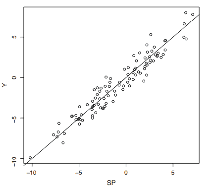
If the unimodal MLR model as estimated by least squares is useful, then in the response plot the plotted points should scatter about the identity line while in the residual plot of $\hat{Y}$ versus $r$ the plotted points should scatter about the $r=0$ line (the horizontal axis) with no other pattern. Figures $1.2$ and $1.3$ show what a response plot and residual plot look like for an artificial MLR data set where the MLR regression relationship is rather strong in that the sample correlation $\operatorname{corr}(\tilde{Y}, Y)$ is near 1 . Figure $1.4$ shows a response plot where the response $Y$ is independent of the nontrivial predictors in the model. Here $\operatorname{corr}(\hat{Y}, Y)$ is near 0 but the points still scatter about the identity line. When the MLR relationship is very weak, the response plot will look like the residual plot.
统计代写|线性回归代写linear regression代考|Checking Lack of Fit
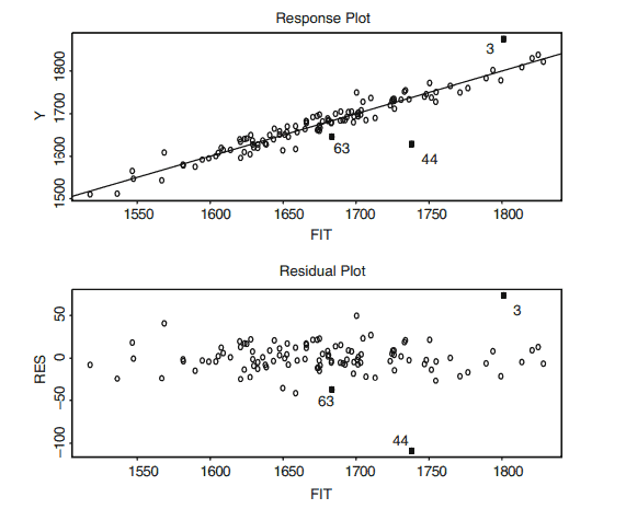
The response plot may look good while the residual plot suggests that the unimodal MLR model can be improved. Examining plots to find model violations is called checking for lack of fit. Again assume that $n \geq 5 p$.
The unimodal MLR model often provides a useful model for the data, but the following assumptions do need to be checked.
i) Is the MLR model appropriate?
ii) Are outliers present?
iii) Is the error variance constant or nonconstant? The constant variance assumption $\operatorname{VAR}\left(e_i\right) \equiv \sigma^2$ is known as homoscedasticity. The nonconstant variance assumption $\operatorname{VAR}\left(e_i\right)=\sigma_i^2$ is known as heteroscedasticity.
iv) Are any important predictors left out of the model?
v) Are the errors $e_1, \ldots, e_n$ iid?
vi) Are the errors $e_i$ independent of the predictors $\boldsymbol{x}_i$ ?
Make the response plot and the residual plot to check i), ii), and iii). An MLR model is reasonable if the plots look like Figures 1.2, 1.3, 1.4, and 2.1. A response plot that looks like Figure $13.7$ suggests that the model is not linear. If the plotted points in the residual plot do not scatter about the $r=0$ line with no other pattern (i.e., if the cloud of points is not ellipsoidal or rectangular with zero slope), then the unimodal MLR model is not sustained.
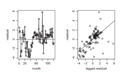
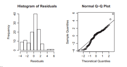
The $i$ th residual $r_i$ is an estimator of the $i$ th error $e_i$. The constant variance assumption may have been violated if the variability of the point cloud in the residual plot depends on the value of $\hat{Y}$. Often the variability of the residuals increases as $\hat{Y}$ increases, resulting in a right opening megaphone shape. (Figure $4.1 \mathrm{~b}$ has this shape.) Often the variability of the residuals decreases as $\hat{Y}$ increases, resulting in a left opening megaphone shape. Sometimes the variability decreases then increases again, and sometimes the variability increases then decreases again (like a stretched or compressed football).
线性回归代写
统计代写|线性回归代写线性回归代考|检验拟合优度
重要的是要认识到MLR模型不一定是数据的有用模型,即使数据集由一个响应变量和几个预测变量组成。例如,可能需要一个非线性回归模型或一个更复杂的模型。第1章和第13章描述了几种替代模型。设$p$为预测数,$n$为病例数。假设$n \geq 5 p$,那么可以使用图来检查MLR模型对研究数据是否有用。这种技术被称为检查MLR模型的拟合优度
符号。图将用于简化回归分析,在本文中$W$与$Z$的图使用$W$作为横轴,$Z$作为纵轴。
定义$X$ vs . $Y$的散点图是$X$ vs . $Y$的散点图,用于可视化给定$X$时$Y$的条件分布$Y \mid X$
定义响应图是一个变量$w_i$和$Y_i$的图。通常$w_i$是预测器的线性组合:$w_i=\boldsymbol{x}_i^T \boldsymbol{\eta}$,其中$\boldsymbol{\eta}$是已知的$p \times 1$向量。最常用的响应曲线是拟合值$\widehat{Y}_i$与响应$Y_i$的曲线。
假设用$\boldsymbol{\beta}$的回归估计量$\boldsymbol{b}$求残差$r_i \equiv r_i(\boldsymbol{b})$和拟合值$\widehat{Y}_i \equiv \widehat{Y}_i(\boldsymbol{b})=\boldsymbol{x}_i^T \boldsymbol{b}$。然后在$\widehat{Y}_i$对$Y_i$的响应图中,与恒等线(具有单位斜率和零截距)的垂直偏差为残差$r_i(b)$ .
证明。响应图中的标识线是$Y=\boldsymbol{x}^T \boldsymbol{b}$。因此垂直偏差为$Y_i-\boldsymbol{x}_i^T \boldsymbol{b}=r_i(\boldsymbol{b})$ .
定义残差图是一个变量$w_i$和残差$r_i$的图。最常用的残差图是$\hat{Y}_i$对$r_i$的残差图
符号:对于MLR,“残差图”通常表示$\hat{Y}_i$对$r_i$的残差图,“响应图”通常表示$\hat{Y}_i$对$Y_i^*$的残差图
如果由最小二乘估计的单峰MLR模型是有用的,那么在响应图中,绘制的点应该分散在标识线附近,而在$\hat{Y}$对$r$的残差图中,绘制的点应该分散在$r=0$线(水平轴)附近,没有其他模式。图$1.2$和$1.3$显示了人工MLR数据集的响应图和残差图,其中MLR回归关系相当强,因为样本相关性$\operatorname{corr}(\tilde{Y}, Y)$接近1。图$1.4$显示了响应图,其中响应$Y$独立于模型中的非平凡预测器。这里$\operatorname{corr}(\hat{Y}, Y)$接近0,但点仍然分散在恒等线上。当MLR关系很弱时,响应图看起来像残差图
统计代写|线性回归代写线性回归代考|检查不符合
. . . .
响应图可能看起来不错,而残差图表明单峰MLR模型可以改进。检查图以发现模型违反称为检查缺乏拟合。再次假设$n \geq 5 p$ .
单峰MLR模型通常为数据提供了一个有用的模型,但需要检查以下假设:
i) MLR模型是否合适?
ii)是否存在异常值?
iii)误差方差是常数还是非常数?恒定方差假设 $\operatorname{VAR}\left(e_i\right) \equiv \sigma^2$ 被称为同异性。非常数方差假设 $\operatorname{VAR}\left(e_i\right)=\sigma_i^2$
iv)模型中是否遗漏了任何重要的预测因子?
v)是否存在误差 $e_1, \ldots, e_n$
vi)错误 $e_i$ 独立于预测因子 $\boldsymbol{x}_i$ ?
绘制响应图和残差图,以检验i), ii)和iii)。如果图如图1.2,1.3,1.4和2.1所示,则MLR模型是合理的。响应图如图所示 $13.7$ 说明模型不是线性的。如果残差图中的点不分散在 $r=0$ 没有其他模式(即,如果点云不是椭球形或斜率为零的矩形),则单峰MLR模型不成立。
$i$ 残差 $r_i$ 的估计值 $i$ 错误 $e_i$。如果残差图中点云的可变性取决于的值,则可能违反恒定方差假设 $\hat{Y}$。通常残差的可变性会随着 $\hat{Y}$ 增加,导致右开口扩音器形状。(图 $4.1 \mathrm{~b}$ 有这个形状。)残差的变异性往往随着 $\hat{Y}$ 增加,导致左侧开口扩音器形状。有时可变性会减小然后再次增大,有时可变性会增大然后再次减小(就像一个拉伸或压缩的足球)

统计代写请认准statistics-lab™. statistics-lab™为您的留学生涯保驾护航。
金融工程代写
金融工程是使用数学技术来解决金融问题。金融工程使用计算机科学、统计学、经济学和应用数学领域的工具和知识来解决当前的金融问题,以及设计新的和创新的金融产品。
非参数统计代写
非参数统计指的是一种统计方法,其中不假设数据来自于由少数参数决定的规定模型;这种模型的例子包括正态分布模型和线性回归模型。
广义线性模型代考
广义线性模型(GLM)归属统计学领域,是一种应用灵活的线性回归模型。该模型允许因变量的偏差分布有除了正态分布之外的其它分布。
术语 广义线性模型(GLM)通常是指给定连续和/或分类预测因素的连续响应变量的常规线性回归模型。它包括多元线性回归,以及方差分析和方差分析(仅含固定效应)。
有限元方法代写
有限元方法(FEM)是一种流行的方法,用于数值解决工程和数学建模中出现的微分方程。典型的问题领域包括结构分析、传热、流体流动、质量运输和电磁势等传统领域。
有限元是一种通用的数值方法,用于解决两个或三个空间变量的偏微分方程(即一些边界值问题)。为了解决一个问题,有限元将一个大系统细分为更小、更简单的部分,称为有限元。这是通过在空间维度上的特定空间离散化来实现的,它是通过构建对象的网格来实现的:用于求解的数值域,它有有限数量的点。边界值问题的有限元方法表述最终导致一个代数方程组。该方法在域上对未知函数进行逼近。[1] 然后将模拟这些有限元的简单方程组合成一个更大的方程系统,以模拟整个问题。然后,有限元通过变化微积分使相关的误差函数最小化来逼近一个解决方案。
tatistics-lab作为专业的留学生服务机构,多年来已为美国、英国、加拿大、澳洲等留学热门地的学生提供专业的学术服务,包括但不限于Essay代写,Assignment代写,Dissertation代写,Report代写,小组作业代写,Proposal代写,Paper代写,Presentation代写,计算机作业代写,论文修改和润色,网课代做,exam代考等等。写作范围涵盖高中,本科,研究生等海外留学全阶段,辐射金融,经济学,会计学,审计学,管理学等全球99%专业科目。写作团队既有专业英语母语作者,也有海外名校硕博留学生,每位写作老师都拥有过硬的语言能力,专业的学科背景和学术写作经验。我们承诺100%原创,100%专业,100%准时,100%满意。
随机分析代写
随机微积分是数学的一个分支,对随机过程进行操作。它允许为随机过程的积分定义一个关于随机过程的一致的积分理论。这个领域是由日本数学家伊藤清在第二次世界大战期间创建并开始的。
时间序列分析代写
随机过程,是依赖于参数的一组随机变量的全体,参数通常是时间。 随机变量是随机现象的数量表现,其时间序列是一组按照时间发生先后顺序进行排列的数据点序列。通常一组时间序列的时间间隔为一恒定值(如1秒,5分钟,12小时,7天,1年),因此时间序列可以作为离散时间数据进行分析处理。研究时间序列数据的意义在于现实中,往往需要研究某个事物其随时间发展变化的规律。这就需要通过研究该事物过去发展的历史记录,以得到其自身发展的规律。
回归分析代写
多元回归分析渐进(Multiple Regression Analysis Asymptotics)属于计量经济学领域,主要是一种数学上的统计分析方法,可以分析复杂情况下各影响因素的数学关系,在自然科学、社会和经济学等多个领域内应用广泛。
MATLAB代写
MATLAB 是一种用于技术计算的高性能语言。它将计算、可视化和编程集成在一个易于使用的环境中,其中问题和解决方案以熟悉的数学符号表示。典型用途包括:数学和计算算法开发建模、仿真和原型制作数据分析、探索和可视化科学和工程图形应用程序开发,包括图形用户界面构建MATLAB 是一个交互式系统,其基本数据元素是一个不需要维度的数组。这使您可以解决许多技术计算问题,尤其是那些具有矩阵和向量公式的问题,而只需用 C 或 Fortran 等标量非交互式语言编写程序所需的时间的一小部分。MATLAB 名称代表矩阵实验室。MATLAB 最初的编写目的是提供对由 LINPACK 和 EISPACK 项目开发的矩阵软件的轻松访问,这两个项目共同代表了矩阵计算软件的最新技术。MATLAB 经过多年的发展,得到了许多用户的投入。在大学环境中,它是数学、工程和科学入门和高级课程的标准教学工具。在工业领域,MATLAB 是高效研究、开发和分析的首选工具。MATLAB 具有一系列称为工具箱的特定于应用程序的解决方案。对于大多数 MATLAB 用户来说非常重要,工具箱允许您学习和应用专业技术。工具箱是 MATLAB 函数(M 文件)的综合集合,可扩展 MATLAB 环境以解决特定类别的问题。可用工具箱的领域包括信号处理、控制系统、神经网络、模糊逻辑、小波、仿真等。