STAT 471 - 统计代写答疑辅导

标签： STAT 471

统计代写|R代写project|Alternate Methods of Numerical Differentiation

Posted on 2022年5月4日2022年5月4日 by statistics-lab

如果你也在怎样代写R这个学科遇到相关的难题，请随时右上角联系我们的24/7代写客服。

R是一个用于统计计算和图形的自由软件环境。

statistics-lab™ 为您的留学生涯保驾护航在代写R方面已经树立了自己的口碑, 保证靠谱, 高质且原创的统计Statistics代写服务。我们的专家在代写R代写方面经验极为丰富，各种代写R相关的作业也就用不着说。

我们提供的R及其相关学科的代写，服务范围广, 其中包括但不限于:

Statistical Inference 统计推断
Statistical Computing 统计计算
Advanced Probability Theory 高等楖率论
Advanced Mathematical Statistics 高等数理统计学
(Generalized) Linear Models 广义线性模型
Statistical Machine Learning 统计机器学习
Longitudinal Data Analysis 纵向数据分析
Foundations of Data Science 数据科学基础

统计代写|R代写project|Alternate Methods of Numerical Differentiation

统计代写|R代写project|Test of dss044

$#$

Test problems, dss004, dss044

$#$

Delete previous workspaces

$\operatorname{rm}($ list $=1 s(a l 1=$ TRUE) )
$#$

Access dss004, dss044 for numerical derivatives

$#$ Test problems, dss004, dss044
$#$ # Delete previous workspaces
rm(list=ls(all=TRUE))
$#$
$#$ Access dss004, dss044 for numerical derivatives
setwd(“f:/appA2”);
source (“dss004.R”);
source(“dss044. $\left.\mathrm{R}^{\prime \prime}\right) ;$
$#$ #
setwd (“f:/appA2”);
source (“dss004. $\mathrm{R}^{\prime \prime}$ );
source (“dss044.R”);
$#$

Arrays for test function, exact (analytical)

derivatives

$\mathrm{n}=11$;
$\mathrm{u}=\operatorname{rep}(0, \mathrm{n})$;
uxa $=\operatorname{rep}(0, \mathrm{n})$;
uxxa $=\operatorname{rep}(0, n)$;
$\operatorname{errx}=\operatorname{rep}(0, \mathrm{n})$;
errxx $=$ rep $(0, n)$;
$#$

Independent variable

$\mathrm{xl}=0 ; \mathrm{xu}=1 ; \mathrm{dx}=(\mathrm{xu}-\mathrm{xl}) /(\mathrm{n}-1)$;
$\mathrm{x}=\operatorname{seq}($ from $=\mathrm{xl}$, to $=\mathrm{xu}, \mathrm{by}=\mathrm{dx})$;
$#$

Select case

for (ncase in $1: 2){$
$#$
$# u x$
for (i in $1: n$ ) {
if $($ ncase $==1){u[i]=\exp (x[i]) ;}$
if $($ ncase $==2){u[i]=\sin (2 * p i \star x[i]) ;}$
}
$u x n=d s s 004(x l, x u, n, u)$;
if (ncase $==1){$
cat (sprintf(” $\backslash \mathrm{n} \backslash \mathrm{n}$ ncase $=\frac{\circ}{\circ} 1 \mathrm{~d}, \mathrm{n}=\stackrel{\circ}{\mathrm{o}} 2 \mathrm{~d}$, dss004″,
ncase, n)) ;
cat (sprintf(
” $\backslash \mathrm{n}$ i $\mathrm{x}$ uxn uxa
errx”));
for (i in $1: n){$
uxa [i] $=\exp (x[i])$;
$\operatorname{errx}[i]=a b s(u x n[i])-a b s$ (uxa [i]);
cat (sprinte (
$i, x[i], \operatorname{uxn}[i], u x a[i], \operatorname{errx}[i])) ;}$
}
if $($ ncase $==2){$
cat (sprintf(” $\backslash \mathrm{n} \backslash \mathrm{n}$ ncase $=\stackrel{\circ}{\circ} 1 \mathrm{~d}, \mathrm{n}=\stackrel{\circ}{\mathrm{z}} 2 \mathrm{~d}, \mathrm{dss004″,}$
ncase, n)) ;
cat (sprintf!
“\n i $x$ uxn uxa
errx”));
for (i in $1: n$ ) {
uxa $[i]=2 * p i \star \cos (2 * p i * x[i])$;
errx[i] =abs (uxn [i])-abs (uxa [i]);

统计代写|R代写project|The independent variable

The independent variable $x$ is defined on an interval with $\mathrm{n}=11$ points, $x_{l}=0 \leq$ $x \leq x_{u}=1$ by the R seq utility.
$#$

Independent variable

$\mathrm{xl}=0 ; \mathrm{xu}=1 ; \mathrm{dx}=(\mathrm{xu}-\mathrm{xl}) /(\mathrm{n}-1)$;
$x=\operatorname{seq}($ from $=x l$, to=xu, by=dx) ;

The programming steps through two cases corresponding to the two test functions, (1) $u(x)=e^{x},(2) u(x)=\sin (2 \pi x)$.
#
# Select case
for (ncase in $1: 2){$
The two test functions are placed in array u.
$#$

ux

for (i in $1: n$ ) {
if $($ ncase $==1){u[i]=\exp (x[i]) ;}$
if (ncase $==2){u[i]=\sin (2 * p i * x[i]) ;}$
}

The first numerical derivative, uxn, is computed for the first function (ncase $=1$ ), and the error in this numerical derivative is computed as the difference of the numerical and exact derivatives, errx [i] =abs (uxn [i])-abs (uxa [i]).
$u x n=d s s 004(x l, x u, n, u)$;
if (ncase $==1$ ) {
cat (sprintf (
” $\backslash \mathrm{n}$ i $\mathrm{x}$ uxn uxa
(errx”));
for (i in $1: n){$
uxa [i] $=\exp (x[i])$;
$\operatorname{errx}[i]=a b s(u x n[i])-a b s$ (uxa [i]);
cat (sprintf(
” $\backslash \mathrm{n}$ ๕ั $4 \mathrm{~d}$ ซั.3f문 $10.5 \mathrm{f} \div 10.5 \mathrm{f} \mathrm{~}$
$i, x[i], u \times n[i]$, uxa [i], errx[i])) i}
}
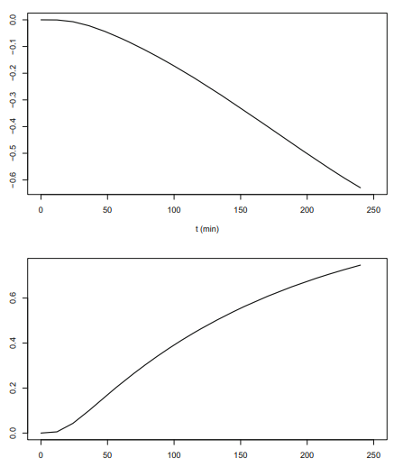
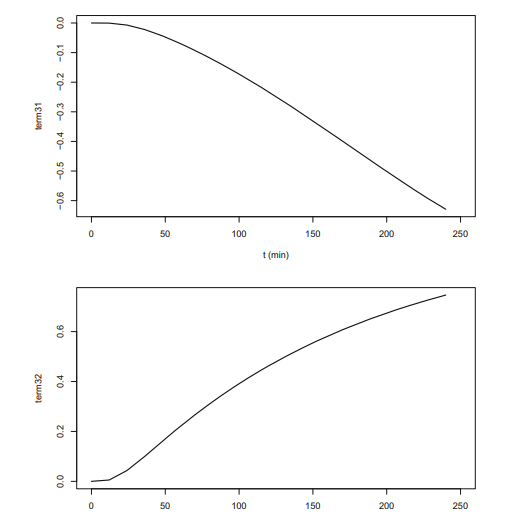
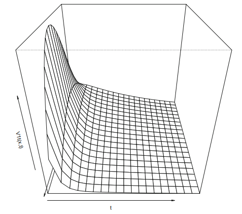
The output displays $x$, the numerical and exact first derivatives, uxn, uxa, and the error in the numerical derivative, errx,

统计代写|R代写project|dss044 Listing

A listing of function dss04 4 follows.
dss044 function $(x l, x u, n, u, u x, n 1, n u)}$
$#$

The derivation of the finite difference

approximations for a second derivative are

in Schiesser, W. E., The Numerical Method

of Lines Integration of Partial Differential

Equations, Academic Press, San Diego, $1991 .$

Preallocate arrays

$u x \times=r e p(0, n)$;
$#$

Grid spacing

$\mathrm{dx}=(\mathrm{xu}-\mathrm{xl}) /(\mathrm{n}-1)$;
$#$
$# 1 /(12 * \mathrm{dx} * \star 2)$ for subsequent use
$r 12 d x s=1 /\left(12 * d x^{\wedge} 2\right)$;
$#$

uxx vector

$#$

Boundaries $(\mathrm{x}=\mathrm{x} l, \mathrm{x}=\mathrm{xu})$

if $(\mathrm{nl}==1)$
uxx $[1]=r 12 d x s *$
$\left(\begin{array}{ll}45 * u[1 & 1\end{array}\right]-154 * u[\quad 2]+214 * u\left[\begin{array}{ll}3 & 3\end{array}\right]-$
$\left.156 * u[4]+61 * u\left[\begin{array}{ll}5 & 5\end{array}\right]-10 * u[6]\right)$;
if $(n u==1)$
uxx $[n]=r 12 d x s *$
$(45 * u[n]-154 * u[n-1]+214 * u[n-2]-$
$156 * u[n-3]+61 * u[n-4]-10 * u[n-5]) ;$
if $(n l==2)$
uxx [1] $=r 12 \mathrm{dxs} *$
$\left(\begin{array}{ll}-415 / 6 * u[1 & 1\end{array}\right]+96 * u[2]-36 * u[1]$
$32 / 3 * u[\quad 4]-3 / 2 * u[\quad 5]-50 * u x[1] * d x)$;
if $(n u==2)$
uXx $[n]=r 12 d x s *$

R代考

统计代写|R代写project|Test of dss044

测试问题，dss004，dss044

删除以前的工作区

R M⁡(列表=1s(一种l1=真的））
##

访问 dss004、dss044 获取数值导数

##测试问题，dss004，dss044
### 删除之前的工作区
rm(list=ls(all=TRUE))
##
##访问 dss004、dss044 获取数值导数
setwd(“f:/appA2”);
来源（“dss004.R”）；
来源（“dss044.R′′);
###
setwd (“f:/appA2”);
来源（“dss004.R′′);
来源（“dss044.R”）；
##

用于测试函数的数组，精确（分析）

衍生品

n=11;
在=代表⁡(0,n);
乌萨=代表⁡(0,n);
乌萨=代表⁡(0,n);
错误=代表⁡(0,n);
错误=代表(0,n);
##

自变量

Xl=0;X在=1;dX=(X在−Xl)/(n−1);
X=序列⁡(从=Xl，到=X在,b是=dX);
##

选择案例

for (ncase in $1: 2){## 用户体验F这r(一世一世n1：n)一世F$($nC一种s和$==1)在[一世]=经验⁡(X[一世]);$一世F$($nC一种s和$==2)在[一世]=罪⁡(2∗p一世⋆X[一世]);$uxn=dss 004(xl, xu, n, u);一世F(nC一种s和==1){C一种吨(spr一世n吨F(”\反斜杠 \mathrm{n} \反斜杠 \mathrm{n}nC一种s和= \ frac {\ circ {\ circ} 1 \ mathrm {~ d}, \ mathrm {n} = \ stackrel {\ circ {\ mathrm {o}} 2 \ mathrm {~ d,dss004″,nC一种s和,n));C一种吨(spr一世n吨F(”\反斜杠 \mathrm{n}一世\数学{x}在Xn在X一种和rrX”));F这r(一世一世n1：n){在X一种[一世]=\exp (x[i]);\operatorname{errx}[i]=abs(uxn[i])-abs(在X一种[一世]);C一种吨(spr一世n吨和(i, x[i], \operatorname{uxn}[i], uxa[i], \operatorname{errx}[i])) ;}} 如果} 如果(nC一种s和==2){C一种吨(spr一世n吨F(”\反斜杠 \mathrm{n} \反斜杠 \mathrm{n}nC一种s和=\stackrel{\circ{\circ}1\mathrm~d},\mathrm{n}=\stackrel\circ}{\mathrm{z}}2\mathrm{~d},\mathrm{dss004″,nC一种s和,n));C一种吨(spr一世n吨F!“\n一世X在Xn在X一种和rrX”));F这r(一世一世n1: n $) {
uxa[一世]=2∗p一世⋆因⁡(2∗p一世∗X[一世]);
errx[i] =abs (uxn [i])-abs (uxa [i]);

统计代写|R代写project|The independent variable

自变量X被定义在一个区间上n=11点，Xl=0≤ X≤X在=1通过 R seq 实用程序。
##

自变量

Xl=0;X在=1;dX=(X在−Xl)/(n−1);
X=序列⁡(从=Xl, to=xu, by=dx) ;

编程步骤通过对应于两个测试功能的两种情况，（1）在(X)=和X,(2)在(X)=罪⁡(2圆周率X).
#
# 选择 case
for (ncase in $1: 2){$
两个测试函数放在数组 u 中。
##

用户体验

对于（我在1:n) {
如果(案例==1)在[一世]=经验⁡(X[一世]);
如果 (ncase==2)在[一世]=罪⁡(2∗p一世∗X[一世]);
}

为第一个函数 (ncase) 计算一阶数值导数 uxn=1)，并且这个数值导数的误差被计算为数值导数和精确导数的差，errx [i] =abs (uxn [i])-abs (uxa [i])。
在Xn=dss004(Xl,X在,n,在);
如果 (ncase==1) {
猫 (sprintf (
”∖n一世Xuxn uxa
(errx”));
对于（我在1: n){$ uxa [i] $=\exp (x[i])$; $\operatorname{errx}[i]=a b s(u x n[i])-a b s$ (uxa [i]); cat (sprintf( ” $\反斜杠 \mathrm{n}$ ๕ั $4 \mathrm{~d}$ ซั.3f문 $10.5 \mathrm{f} \div 10.5 \mathrm{f} \mathrm{~}$ $i , x[i], u \times n[i]$, uxa [i], errx[i])) i} } 输出显示1: n){$ uxa [i] $=\exp (x[i])$; $\operatorname{errx}[i]=a b s(u x n[i])-a b s$ (uxa [i]); cat (sprintf( ” $\反斜杠 \mathrm{n}$ ๕ั $4 \mathrm{~d}$ ซั.3f문 $10.5 \mathrm{f} \div 10.5 \mathrm{f} \mathrm{~}$ $i , x[i], u \times n[i]$, uxa [i], errx[i])) i} } 输出显示x$，数值和精确的一阶导数，uxn，uxa，以及数值导数中的误差，errx，

统计代写|R代写project|dss044 Listing

dss04 4 函数列表如下。
dss044 功能(x l, x u, n, u, u x, n 1, n u)}(x l, x u, n, u, u x, n 1, n u)}
##

有限差分的推导

二阶导数的近似值是

在 Schiesser, WE, 数值方法

线积分的偏微分

方程式，学术出版社，圣地亚哥，1991.

预分配数组

在X×=r和p(0,n);
##

网格间距

dX=(X在−Xl)/(n−1);
##
# 1 /(12 * \mathrm{dx} * \star 2)# 1 /(12 * \mathrm{dx} * \star 2)供后续使用
r12dXs=1/(12∗dX∧2);
##

uxx 矢量图

边界(X=Xl,X=X在)

如果(nl==1)
uxx[1]=r12dXs∗
(45∗在[11]−154∗在[2]+214∗在[33]−
156∗在[4]+61∗在[55]−10∗在[6]);
如果(n在==1)
uxx[n]=r12dXs∗
(45∗在[n]−154∗在[n−1]+214∗在[n−2]−
156∗在[n−3]+61∗在[n−4]−10∗在[n−5]);
如果(nl==2)
uxx [1]=r12dXs∗
(−415/6∗在[11]+96∗在[2]−36∗在[1]
32/3∗在[4]−3/2∗在[5]−50∗在X[1]∗dX);
如果(n在==2)
uXx[n]=r12dXs∗

统计代写请认准statistics-lab™. statistics-lab™为您的留学生涯保驾护航。

金融工程代写

金融工程是使用数学技术来解决金融问题。金融工程使用计算机科学、统计学、经济学和应用数学领域的工具和知识来解决当前的金融问题，以及设计新的和创新的金融产品。

非参数统计代写

非参数统计指的是一种统计方法，其中不假设数据来自于由少数参数决定的规定模型；这种模型的例子包括正态分布模型和线性回归模型。

广义线性模型代考

广义线性模型（GLM）归属统计学领域，是一种应用灵活的线性回归模型。该模型允许因变量的偏差分布有除了正态分布之外的其它分布。

术语广义线性模型（GLM）通常是指给定连续和/或分类预测因素的连续响应变量的常规线性回归模型。它包括多元线性回归，以及方差分析和方差分析（仅含固定效应）。

有限元方法代写

有限元方法（FEM）是一种流行的方法，用于数值解决工程和数学建模中出现的微分方程。典型的问题领域包括结构分析、传热、流体流动、质量运输和电磁势等传统领域。

有限元是一种通用的数值方法，用于解决两个或三个空间变量的偏微分方程（即一些边界值问题）。为了解决一个问题，有限元将一个大系统细分为更小、更简单的部分，称为有限元。这是通过在空间维度上的特定空间离散化来实现的，它是通过构建对象的网格来实现的：用于求解的数值域，它有有限数量的点。边界值问题的有限元方法表述最终导致一个代数方程组。该方法在域上对未知函数进行逼近。[1] 然后将模拟这些有限元的简单方程组合成一个更大的方程系统，以模拟整个问题。然后，有限元通过变化微积分使相关的误差函数最小化来逼近一个解决方案。

tatistics-lab作为专业的留学生服务机构，多年来已为美国、英国、加拿大、澳洲等留学热门地的学生提供专业的学术服务，包括但不限于Essay代写，Assignment代写，Dissertation代写，Report代写，小组作业代写，Proposal代写，Paper代写，Presentation代写，计算机作业代写，论文修改和润色，网课代做，exam代考等等。写作范围涵盖高中，本科，研究生等海外留学全阶段，辐射金融，经济学，会计学，审计学，管理学等全球99%专业科目。写作团队既有专业英语母语作者，也有海外名校硕博留学生，每位写作老师都拥有过硬的语言能力，专业的学科背景和学术写作经验。我们承诺100%原创，100%专业，100%准时，100%满意。

随机分析代写

随机微积分是数学的一个分支，对随机过程进行操作。它允许为随机过程的积分定义一个关于随机过程的一致的积分理论。这个领域是由日本数学家伊藤清在第二次世界大战期间创建并开始的。

时间序列分析代写

随机过程，是依赖于参数的一组随机变量的全体，参数通常是时间。随机变量是随机现象的数量表现，其时间序列是一组按照时间发生先后顺序进行排列的数据点序列。通常一组时间序列的时间间隔为一恒定值（如1秒，5分钟，12小时，7天，1年），因此时间序列可以作为离散时间数据进行分析处理。研究时间序列数据的意义在于现实中，往往需要研究某个事物其随时间发展变化的规律。这就需要通过研究该事物过去发展的历史记录，以得到其自身发展的规律。

回归分析代写

多元回归分析渐进（Multiple Regression Analysis Asymptotics）属于计量经济学领域，主要是一种数学上的统计分析方法，可以分析复杂情况下各影响因素的数学关系，在自然科学、社会和经济学等多个领域内应用广泛。

MATLAB代写

MATLAB 是一种用于技术计算的高性能语言。它将计算、可视化和编程集成在一个易于使用的环境中，其中问题和解决方案以熟悉的数学符号表示。典型用途包括：数学和计算算法开发建模、仿真和原型制作数据分析、探索和可视化科学和工程图形应用程序开发，包括图形用户界面构建MATLAB 是一个交互式系统，其基本数据元素是一个不需要维度的数组。这使您可以解决许多技术计算问题，尤其是那些具有矩阵和向量公式的问题，而只需用 C 或 Fortran 等标量非交互式语言编写程序所需的时间的一小部分。MATLAB 名称代表矩阵实验室。MATLAB 最初的编写目的是提供对由 LINPACK 和 EISPACK 项目开发的矩阵软件的轻松访问，这两个项目共同代表了矩阵计算软件的最新技术。MATLAB 经过多年的发展，得到了许多用户的投入。在大学环境中，它是数学、工程和科学入门和高级课程的标准教学工具。在工业领域，MATLAB 是高效研究、开发和分析的首选工具。MATLAB 具有一系列称为工具箱的特定于应用程序的解决方案。对于大多数 MATLAB 用户来说非常重要，工具箱允许您学习和应用专业技术。工具箱是 MATLAB 函数（M 文件）的综合集合，可扩展 MATLAB 环境以解决特定类别的问题。可用工具箱的领域包括信号处理、控制系统、神经网络、模糊逻辑、小波、仿真等。

R语言代写	问卷设计与分析代写
PYTHON代写	回归分析与线性模型代写
MATLAB代写	方差分析与试验设计代写
STATA代写	机器学习/统计学习代写
SPSS代写	计量经济学代写
EVIEWS代写	时间序列分析代写
EXCEL代写	深度学习代写
SQL代写	各种数据建模与可视化代写

统计代写|R代写project|Function dss004

Posted on 2022年5月4日2022年5月4日 by statistics-lab

如果你也在怎样代写R这个学科遇到相关的难题，请随时右上角联系我们的24/7代写客服。

R是一个用于统计计算和图形的自由软件环境。

我们提供的R及其相关学科的代写，服务范围广, 其中包括但不限于:

Statistical Inference 统计推断
Statistical Computing 统计计算
Advanced Probability Theory 高等楖率论
Advanced Mathematical Statistics 高等数理统计学
(Generalized) Linear Models 广义线性模型
Statistical Machine Learning 统计机器学习
Longitudinal Data Analysis 纵向数据分析
Foundations of Data Science 数据科学基础

统计代写|R代写project|dss004 listing

A listing of function dss0 04 follows.
dss004 =function $(x 1, x u, n, u) \quad{$
$#$

An extensive set of documentation comments detailing

the derivation of the following fourth order finite

differences (FDs) is not given here to conserve

space. The derivation is detailed in schiesser,

W. E., The Numerical Method of Lines Integration

of Partial Differential Equations, Academic Press,

San Diego, $1991 .$

$#$

Preallocate arrays

$u x=r e p(0, n)$;
$#$

Grid spacing

$d x=(x u-x l) /(n-1)$;
#

$1 /(12 * d x)$ for subsequent use

$r 12 \mathrm{dx}=1 /(12 * \mathrm{dx})$;
#

ux vector

Boundaries ( $\mathrm{x}=\mathrm{xl}, \mathrm{x}=\mathrm{xu})$

$u x[1]=r 12 d x *\left(-25 * u[1]+48 * u\left[\begin{array}{ll}1 & 2\end{array}\right]-36 * u\left[\begin{array}{ll} & 3\end{array}\right]+16 * u\left[\begin{array}{l}4\end{array}\right]\right.$
$-3 * u[5])$;
$u x[n]=r 12 d x *(25 * u[n]-48 * u[n-1]+36 * u[n-2]-16 * u[n-3]$

统计代写|R代写project|Test of dss004

The following main program includes the calls to dss 004 .
#

Test problems, dss004

$#$

Delete previous workspaces

$\operatorname{rm}(1$ ist =ls (all=TRUE))
$#$

Access dss004 for numerical derivatives

setwd (“f:/vci/appA1”);
source (“dss004. $R^{\prime \prime}$ );
$#$

Arrays for test function, exact (analytical)

derivatives

$n=11$;
$\mathrm{u}=\operatorname{rep}(0, \mathrm{n})$;
$u x a=r e p(0, n)$;
uxxa $=r e p(0, n)$;
errx $=r e p(0, n)$;
$\operatorname{errxx}=\operatorname{rep}(0, \mathrm{n})$;
$#$

Independent variable

$\mathrm{xl}=0 ; \mathrm{xu}=1 ; \mathrm{dx}=(\mathrm{xu}-\mathrm{xl}) /(\mathrm{n}-1)$;
$\mathrm{x}=\operatorname{seq}($ from $=\mathrm{xl}$, to $=\mathrm{xu}, \mathrm{by}=\mathrm{dx})$;
$#$

Select case

for (ncase in $1: 2){$
$#$

统计代写|R代写project|Function dss004

We can note the following details about this output.

The error is substantially larger at the end values of $x$, e.g., compare the errors at $x=0$ and $x=0.1$.
The accuracy of the numerical derivatives decreases with successive differentiations, e.g., the preceding numerical output indicates the second numerical derivative has lower accuracy then the first numerical derivative (the two derivatives can be compared numerically since they are the same for $\left.u(x)=e^{x}\right)$.
These features of the numerical output are reflected in the graphical output of Figs. A2.1 that include Figs. A2.1-1, A2.1-2

The errors in the numerical derivatives, particularly at the end points $x=x_{l}=0$, $x=x_{u}=1$, and the gridding effects (nonsmooth variation with $x$ ) for $n=11$ are apparent in Fig. A 1.1-2.
In summary, we can note

The lower accuracy at the end points, $x=x_{l}=0, x=x_{u t}=1$.
The linear interpolation between points as provided by plot.
The nonsmooth numerical solutions for $\frac{d u(x)}{d x}, \frac{d^{2} u(x)}{d x^{2}}$ which is a gridding effect for $n=11$ as demonstrated in subsequent solutions (by increasing $n$ ).

R代考

统计代写|R代写project|dss004 listing

函数 dss0 04 的列表如下。
dss004 = 函数 $(x 1, xu, n, u) \quad{#$

一组广泛的文档注释详细说明

以下四阶有限的推导

此处未给出差异（FD）以节省

空间。推导在 schiesser 中有详细说明，

WE，线积分的数值方法

偏微分方程，学术出版社，

圣地亚哥，1991.

预分配数组

在X=r和p(0,n);
##

网格间距

dX=(X在−Xl)/(n−1);
#

1/(12∗dX)后续使用

r12dX=1/(12∗dX);
#

用户体验矢量图

边界（X=Xl,X=X在)

在X[1]=r12dX∗(−25∗在[1]+48∗在[12]−36∗在[3]+16∗在[4]
−3∗在[5]);
在X[n]=r12dX∗(25∗在[n]−48∗在[n−1]+36∗在[n−2]−16∗在[n−3]

统计代写|R代写project|Test of dss004

以下主程序包括对 dss 004 的调用。
#

测试问题，dss004

删除以前的工作区

R M⁡(1ist =ls (all=TRUE))
##

访问 dss004 获取数值导数

setwd (“f:/vci/appA1”);
来源（“dss004.R′′ );
##

用于测试函数的数组，精确（分析）

衍生品

n=11;
在=代表⁡(0,n);
在X一种=r和p(0,n);
乌萨=r和p(0,n);
错误=r和p(0,n);
错误=代表⁡(0,n);
##

自变量

Xl=0;X在=1;dX=(X在−Xl)/(n−1);
X=序列⁡(从=Xl，到=X在,b是=dX);
##

选择案例

for (ncase in $1: 2){#$

统计代写|R代写project|Function dss004

我们可以注意到有关此输出的以下详细信息。

最终值的误差要大得多X，例如，比较错误X=0和X=0.1.
数值导数的精度随着连续微分而降低，例如，前面的数值输出表明二阶数值导数的精度低于一阶数值导数（这两个导数可以在数值上进行比较，因为它们对于在(X)=和X).
数值输出的这些特征反映在图 1 和图 3 的图形输出中。A2.1 包括无花果。A2.1-1、A2.1-2

数值导数中的误差，特别是在端点处X=Xl=0, X=X在=1，以及网格化效果（非平滑变化与X）为了n=11在图 A 1.1-2 中很明显。
总之，我们可以注意到

端点的精度较低，X=Xl=0,X=X在吨=1.
plot 提供的点之间的线性插值。
的非光滑数值解d在(X)dX,d2在(X)dX2这是一个网格效果n=11如后续解决方案所示（通过增加n ).

统计代写请认准statistics-lab™. statistics-lab™为您的留学生涯保驾护航。

金融工程代写

非参数统计代写

非参数统计指的是一种统计方法，其中不假设数据来自于由少数参数决定的规定模型；这种模型的例子包括正态分布模型和线性回归模型。

广义线性模型代考

广义线性模型（GLM）归属统计学领域，是一种应用灵活的线性回归模型。该模型允许因变量的偏差分布有除了正态分布之外的其它分布。

有限元方法代写

随机分析代写

时间序列分析代写

回归分析代写

MATLAB代写

R语言代写	问卷设计与分析代写
PYTHON代写	回归分析与线性模型代写
MATLAB代写	方差分析与试验设计代写
STATA代写	机器学习/统计学习代写
SPSS代写	计量经济学代写
EVIEWS代写	时间序列分析代写
EXCEL代写	深度学习代写
SQL代写	各种数据建模与可视化代写

统计代写|R代写project|ODE/PDE routine

Posted on 2022年5月4日2022年5月4日 by statistics-lab

如果你也在怎样代写R这个学科遇到相关的难题，请随时右上角联系我们的24/7代写客服。

R是一个用于统计计算和图形的自由软件环境。

我们提供的R及其相关学科的代写，服务范围广, 其中包括但不限于:

Statistical Inference 统计推断
Statistical Computing 统计计算
Advanced Probability Theory 高等楖率论
Advanced Mathematical Statistics 高等数理统计学
(Generalized) Linear Models 广义线性模型
Statistical Machine Learning 统计机器学习
Longitudinal Data Analysis 纵向数据分析
Foundations of Data Science 数据科学基础

统计代写|R代写project|Numerical, graphical output

The numerical output is the same as in Table 3.1. Also, the graphical output for $C_{1}(t), C_{2}(t), C_{3}(t)$ is the same as in Figs. 3.1-2,3.1-4 and is not repeated here. The graphical output for the RHS terms and LHS derivatives of eqs. $(5.1-1),(5.2-1),(5.3-1)$ is in Figs. $5.2$.
The plots for $\frac{\partial V_{3}(x, t)}{\partial t}$ are the same as for $\frac{\partial V_{2}(x, t)}{\partial t}$ and are not included here.
Generally, Figs. $5.2$ indicate the approach of the solutions to a stable, steady state.
To conclude this discussion of the analysis of the PDEs, eqs. $(5.1-1),(5.2-1)$, (5.3-1), the following code is added to Listing $5.2$.
$#$

Plot PDE derivative terms

V1t

matplot $\left(\mathrm{x}=\mathrm{x}, \mathrm{y}=\operatorname{term} 11[, 2\right.$ : nout $]$, type $={ }^{\prime \prime} 1^{\prime \prime}, \mathrm{xlab}={ }^{\prime \prime} \mathrm{x}$, ,
$y l a b=” t e r m 11^{\prime \prime}, x l i m=c(x l, x u), l t y=1$, main=” “, lwd=2,
col = “black”) ;
$\operatorname{persp}(\mathrm{x}$, tout [ 2 : nout], term11 [, 2 : nout], theta $=90$, phi=30,
$x l i m=c(x l, x u), y l i m=c(t 0, t f), x l a b=” x$ “,
$\left.y l a b={ }^{n \prime \prime}, z l a b=” \operatorname{term} 11^{\prime \prime}\right)$;
$#$
$# \mathrm{~V} 2 \mathrm{t}$
$\operatorname{par}(\operatorname{mfrow}=\mathrm{C}(2,2))$;
matplot $\left(\mathrm{x}=\mathrm{x}, \mathrm{y}=\operatorname{term} 21\right.$, type $=” 1 “, \mathrm{xlab}={ }^{\prime \prime} \mathrm{x}^{\mathrm{n}}, \mathrm{ylab}=$ “term21”,
$x l i m=c(x l, x u), 1 t y=1$, main=” , lwd=2, col= “black”);
matplot $\left(\mathrm{x}=\mathrm{x}, \mathrm{y}=\operatorname{term} 22\right.$, type $=” 1 “, \mathrm{xlab}={ }^{\prime \prime} \mathrm{x}^{\mathrm{n}}, \mathrm{ylab}=$ “term 22 “,
$x l i m=c(x l, x u), 1 t y=1$, main=” , $1 w d=2$, col= “black”);
matplot $\left(\mathrm{x}=\mathrm{x}, \mathrm{Y}=\operatorname{term} 21+\operatorname{term} 22\right.$, type $={ }^{\prime \prime} 1^{\prime \prime}, \mathrm{xlab}=$ ” $\mathrm{x}$ “,
$y l a b=” \operatorname{term} 21+\operatorname{term} 22 “, x l i m=c(x l, x u)$, lty=1, main=” “,
$1 w \mathrm{~d}=2, \mathrm{col}=$ ” $\mathrm{black}$ “);
$\operatorname{par}(\operatorname{mfrow}=\mathrm{c}(2,2))$;
persp $(\mathrm{x}$, tout, term 21 , theta $=30$, phi $=30$,
$x l i m=c(x l, x u), y l i m=c(t 0, t f), x l a b=” x^{\prime \prime}$,
ylab=” ” “,$\left.z l a b=” \operatorname{term} 21^{\prime \prime}\right)$;
persp ( $x$, tout, term 22 , theta $=30$, phi $=30$,
$x l i m=c(x l, x u), y l i m=c(t 0, t f), x l a b={ }^{n} x$ “,

统计代写|R代写project|The RHS terms

The RHS terms of eq. $(5.2-1)$ and their sum are plotted.
$#$

V2t

$\operatorname{par}(\operatorname{mfrow}=\mathrm{C}(2,2))$;
matplot $\left(\mathrm{x}=\mathrm{x}, \mathrm{y}=\operatorname{term} 21, t y p e={ }^{\prime \prime}, \mathrm{x} l \mathrm{ab}={ }^{\prime \prime} \mathrm{x}\right.$,
$y l a b=” \operatorname{term} 21^{\prime \prime}, x l i m=c(x l, x u), 1 t y=1$, main=” , $1 w d=2$,
cOl = “black”);
matplot $(x=x, y=t e r m 22, t y p e=” 1 ” x l a b=” x$,
$y l a b=” \operatorname{term} 22^{\prime \prime}, \mathrm{xlim}=\mathrm{c}(\mathrm{xl}, \mathrm{xu}), 1 \mathrm{ty}=1$, main=” , $1 w \mathrm{~d}=2$,
COl = “black” );
matplot $\left(x=x, y=t e r m 21+t e r m 22, t y p e=” 1 “, x \perp a b={ }^{\prime \prime} x^{n}\right.$,
$Y l a b=$ “term21+term22″, ” $1 \mathrm{~m}=\mathrm{c}(\mathrm{xl}, \mathrm{xu}), 1 \mathrm{t}=1, \mathrm{ma} \mathrm{n}=$ ” $\mathrm{~ , ~}$
$l w \mathrm{~d}=2, \mathrm{col}=” \mathrm{black}$ “) ;
par $(\operatorname{mf} r \mathrm{OW}=\mathrm{C}(2,2))$ i
persp $(x$, tout, term 21 , theta $=30$, phi $=30$,
$x \perp i m=c(x \perp, x u), y \perp i m=c(t 0, t f), x \perp a b=” x “$,
$\left.y l a b=” t^{\prime \prime}, z l a b=” \operatorname{term} 21^{n \prime}\right)$;
persp $(x$, tout, term 22 , theta $=30$, phi $=30$,
$x l i m=c(x l, x u), y l i m=c(t 0, t f), x \perp a b=” x “$,
$\left.y l a b=” t^{\prime \prime}, z l a b=” \operatorname{term} 22^{n}\right)$;
persp $(x$, tout, term $21+\operatorname{term} 22$, theta $=30$, phi $=30$,
$x l i m=c(x \perp, x u), y l i m=c(t 0, t f), x \perp a b=” x “$,
$\left.y l a b=” t^{\prime \prime}, z l a b=” t e r m 21+\operatorname{term} 22^{\prime \prime}\right) ;$

The RHS terms of eq. (5.3-1) and their sum are plotted.
$#$

V3t

$\operatorname{par}(\operatorname{mfrow}=\mathrm{c}(2,2))$;
matplot $\left(\mathrm{x}=\mathrm{x}, \mathrm{Y}=\operatorname{term} 31, \mathrm{type}={ }^{\mathrm{n}} \mathrm{I}^{\prime \prime}, \mathrm{x} \perp \mathrm{ab}={ }^{\prime \prime} \mathrm{x}\right.$,
$Y l a b=” \operatorname{term} 31^{\prime \prime}, \mathrm{xlim}=\mathrm{c}(\mathrm{xl}, \mathrm{xu}), 1 \mathrm{t} y=1$, main=” , $1 w \mathrm{~d}=2$,
$\mathrm{CO}=$ “black”)
matplot $\left(\mathrm{x}=\mathrm{x}, \mathrm{y}=\operatorname{term} 32, \mathrm{ype}=\mathrm{I}^{\prime \prime}, \mathrm{xlab}=\mathrm{x}^{\prime \prime}\right.$,
$y l a b=” \operatorname{term} 32^{\prime \prime}, \mathrm{xlim}=\mathrm{c}(\mathrm{xl}, \mathrm{xu}), 1 \mathrm{ty}=1$, main=” , $1 w \mathrm{~d}=2$,
$\mathrm{COl}=” \mathrm{black}$ “)
matplot $\left(x=x, y=t e r m 31+t e r m 32, t y p e=” 1 “, x \perp a b={ }^{\prime \prime} x^{n}\right.$,
$Y l a b=$ “term $31+\operatorname{term} 32^{\text {n }}, \mathrm{xl} \mathrm{m}=\mathrm{c}(\mathrm{xl}, \mathrm{xu}), 1 \mathrm{t}=1, \mathrm{main=}$, 午,
$I w \mathrm{~d}=2, \mathrm{col}=$ “black”);
$\operatorname{par}(\operatorname{mfrow}=\mathrm{C}(2,2))$;
persp $(x$, tout, term 31 , theta $=30$, phi $=30$,
$\mathrm{xl} \mathrm{m}=\mathrm{c}(\mathrm{xl}, \mathrm{xu}), \mathrm{yl} \mathrm{m}=\mathrm{c}(\mathrm{t} 0, \mathrm{tf}), \mathrm{xlab}={ }^{\prime \prime} \mathrm{x}$,
$y l a b=” t^{\prime \prime}, z l a b=” \operatorname{term} 31^{n \prime}$;

统计代写|R代写project|Summary and conclusions

The ODE/PDE model of eqs. (5.1), (5.2), (5.3) is analyzed in detail by computing and plotting the ODE/PDE RHS terms and the LHS $t$ derivatives. This analysis gives an explanation of the origin of the ODE/PDE model solution properties. The model can now be studied in further detail. For example,

The cross diffusion term in eqs. $(5.2-1),(5.2-2)$ can be expanded as
$$
\frac{\partial^{2}\left(V_{2}(x, t) V_{3}(x, t)\right)}{\partial x^{2}}=
$$

$$
\frac{\partial\left(V_{2}(x, t) \frac{\partial V_{3}(x, t)}{\partial x}\right)}{\partial x}+\frac{\partial\left(V_{3}(x, t) \frac{\partial V_{2}(x, t)}{\partial x}\right)}{\partial x}
$$
The two RHS terms can then be calculated and plotted separately to determine the contributions of each.

The parameters for components 2,3 can be different in Listing 5.1. For example, these components may be of different size (molecular weight) so that the diffusivities $D_{V 2}, D_{V 3}$, and cross diffusion coefficients $\chi_{2}, \chi_{3}$ in eqs. (5.2-1), (5.3-1) are different.
The effect of the mass transfer coefficients $k_{1 l}, k_{1 u}, k_{2 l}, k_{2 u}, k_{3 l}, k_{3 u}$ can be studied, possibly as experimental data for the rate of transfer of viral genetic material into host cells become available.
These suggested investigations are left as exercises.

R代考

统计代写|R代写project|Numerical, graphical output

数值输出与表 3.1 相同。此外，图形输出为C1(吨),C2(吨),C3(吨)与图 2 中的相同。3.1-2,3.1-4，这里不再赘述。eqs 的 RHS 项和 LHS 导数的图形输出。(5.1−1),(5.2−1),(5.3−1)是在无花果。5.2.
的地块∂在3(X,吨)∂吨与∂在2(X,吨)∂吨并且不包括在这里。
一般来说，无花果。5.2表示解决方案接近稳定、稳定的状态。
结束对 PDE 分析的讨论，等式。(5.1−1),(5.2−1), (5.3-1)，在Listing中加入如下代码5.2.
##

绘制 PDE 导数项

V1t

matplot(X=X,是=学期⁡11[,2: 没有]，类型=′′1′′,Xl一种b=′′X, ,
是l一种b=”吨和r米11′′,Xl一世米=C(Xl,X在),l吨是=1, main=” “, lwd=2,
col = “黑色”) ;
透视⁡(X, tout [2:nout], term11 [, 2:nout], theta=90, φ = 30,
Xl一世米=C(Xl,X在),是l一世米=C(吨0,吨F),Xl一种b=”X “,
是l一种b=n′′,和l一种b=”学期⁡11′′);
##
# \ mathrm ~ V} 2 \ mathrm {t# \ mathrm ~ V} 2 \ mathrm {t
关于⁡(mfrow=C(2,2));
matplot(X=X,是=学期⁡21，类型=”1“,Xl一种b=′′Xn,是l一种b=“第 21 学期”，
Xl一世米=C(Xl,X在),1吨是=1, 主 =” , lwd = 2, col = “黑色”);
matplot(X=X,是=学期⁡22，类型=”1“,Xl一种b=′′Xn,是l一种b=“第 22 期”，
Xl一世米=C(Xl,X在),1吨是=1, 主要 =” ,1在d=2，col=“黑色”）；
matplot(X=X,是=学期⁡21+学期⁡22，类型=′′1′′,Xl一种b= ” X “,
是l一种b=”学期⁡21+学期⁡22“,Xl一世米=C(Xl,X在), lty = 1, main = “”,
1在 d=2,C这l=”bl一种Cķ “);
关于⁡(mfrow=C(2,2));
透视(X, tout, 第 21 学期, theta=30, φ=30,
Xl一世米=C(Xl,X在),是l一世米=C(吨0,吨F),Xl一种b=”X′′,
ylab = “” “,和l一种b=”学期⁡21′′);
透视（X, 吹捧, 第 22 学期, theta=30, φ=30,
Xl一世米=C(Xl,X在),是l一世米=C(吨0,吨F),Xl一种b=nX“,

统计代写|R代写project|The RHS terms

等式的 RHS 项。(5.2−1)并绘制它们的总和。
##

V2t

关于⁡(mfrow=C(2,2));
matplot(X=X,是=学期⁡21,吨是p和=′′,Xl一种b=′′X,
是l一种b=”学期⁡21′′,Xl一世米=C(Xl,X在),1吨是=1, 主要 =” ,1在d=2,
col = “黑色”);
matplot(X=X,是=吨和r米22,吨是p和=”1”Xl一种b=”X,
是l一种b=”学期⁡22′′,Xl一世米=C(Xl,X在),1吨是=1, 主要 =” ,1在 d=2,
COl = “黑色” );
matplot(X=X,是=吨和r米21+吨和r米22,吨是p和=”1“,X⊥一种b=′′Xn,
是l一种b=“期限21+期限22”，”1 米=C(Xl,X在),1吨=1,米一种n=” ,
l在 d=2,C这l=”bl一种Cķ“）；
关于(MF⁡r这在=C(2,2))我
相信(X, tout, 第 21 学期, theta=30, φ=30,
X⊥一世米=C(X⊥,X在),是⊥一世米=C(吨0,吨F),X⊥一种b=”X“,
是l一种b=”吨′′,和l一种b=”学期⁡21n′);
透视(X, 吹捧, 第 22 学期, theta=30, φ=30,
Xl一世米=C(Xl,X在),是l一世米=C(吨0,吨F),X⊥一种b=”X“,
是l一种b=”吨′′,和l一种b=”学期⁡22n);
透视(X, 所有, 术语21+学期⁡22, θ=30, φ=30,
Xl一世米=C(X⊥,X在),是l一世米=C(吨0,吨F),X⊥一种b=”X“,
是l一种b=”吨′′,和l一种b=”吨和r米21+学期⁡22′′);

等式的 RHS 项。(5.3-1) 和它们的总和被绘制出来。
##

V3t

关于⁡(mfrow=C(2,2));
matplot(X=X,是=学期⁡31,吨是p和=n一世′′,X⊥一种b=′′X,
是l一种b=”学期⁡31′′,Xl一世米=C(Xl,X在),1吨是=1, 主要 =” ,1在 d=2,
C这=“黑色”）
matplot(X=X,是=学期⁡32,是p和=一世′′,Xl一种b=X′′,
是l一种b=”学期⁡32′′,Xl一世米=C(Xl,X在),1吨是=1, 主要 =” ,1在 d=2,
C这l=”bl一种Cķ”）
matplot(X=X,是=吨和r米31+吨和r米32,吨是p和=”1“,X⊥一种b=′′Xn,
是l一种b=“学期31+学期⁡32n ,Xl米=C(Xl,X在),1吨=1,米一种一世n=, 午,
一世在 d=2,C这l=“黑色的”）;
关于⁡(mfrow=C(2,2));
透视(X, 吹捧, 第 31 学期, theta=30, φ=30,
Xl米=C(Xl,X在),是l米=C(吨0,吨F),Xl一种b=′′X,
是l一种b=”吨′′,和l一种b=”学期⁡31n′;

统计代写|R代写project|Summary and conclusions

方程的 ODE/PDE 模型。通过计算和绘制 ODE/PDE RHS 项和 LHS 对 (5.1)、(5.2)、(5.3) 进行详细分析吨衍生品。该分析解释了 ODE/PDE 模型解属性的起源。现在可以更详细地研究该模型。例如，

方程中的交叉扩散项。(5.2−1),(5.2−2)可以扩展为
∂2(在2(X,吨)在3(X,吨))∂X2=

∂(在2(X,吨)∂在3(X,吨)∂X)∂X+∂(在3(X,吨)∂在2(X,吨)∂X)∂X
然后可以分别计算和绘制这两个 RHS 项，以确定每个项的贡献。

清单 5.1 中组件 2,3 的参数可以不同。例如，这些成分可能具有不同的尺寸（分子量），从而使扩散率D在2,D在3, 和交叉扩散系数χ2,χ3在等式中。(5.2-1)、(5.3-1) 不同。
传质系数的影响ķ1l,ķ1在,ķ2l,ķ2在,ķ3l,ķ3在可以研究，可能随着病毒遗传物质转移到宿主细胞的速率的实验数据变得可用。
这些建议的调查留作练习。

统计代写请认准statistics-lab™. statistics-lab™为您的留学生涯保驾护航。

金融工程代写

非参数统计代写

非参数统计指的是一种统计方法，其中不假设数据来自于由少数参数决定的规定模型；这种模型的例子包括正态分布模型和线性回归模型。

广义线性模型代考

广义线性模型（GLM）归属统计学领域，是一种应用灵活的线性回归模型。该模型允许因变量的偏差分布有除了正态分布之外的其它分布。

有限元方法代写

随机分析代写

时间序列分析代写

回归分析代写

MATLAB代写

R语言代写	问卷设计与分析代写
PYTHON代写	回归分析与线性模型代写
MATLAB代写	方差分析与试验设计代写
STATA代写	机器学习/统计学习代写
SPSS代写	计量经济学代写
EVIEWS代写	时间序列分析代写
EXCEL代写	深度学习代写
SQL代写	各种数据建模与可视化代写

统计代写|R代写project|Detailed ODE

Posted on 2022年5月4日2022年5月4日 by statistics-lab

如果你也在怎样代写R这个学科遇到相关的难题，请随时右上角联系我们的24/7代写客服。

R是一个用于统计计算和图形的自由软件环境。

我们提供的R及其相关学科的代写，服务范围广, 其中包括但不限于:

Statistical Inference 统计推断
Statistical Computing 统计计算
Advanced Probability Theory 高等楖率论
Advanced Mathematical Statistics 高等数理统计学
(Generalized) Linear Models 广义线性模型
Statistical Machine Learning 统计机器学习
Longitudinal Data Analysis 纵向数据分析
Foundations of Data Science 数据科学基础

统计代写|R代写project|PDE Model Analysis

Abstract The right hand side (RHS) terms and left hand side (LHS) time derivatives of the ODE/PDE models of Chapter 3 are computed and displayed to provide additional insight into the origin of the model solution properties. The RHSs and LHSs are computed from the method of lines (MOL) numerical solutions of the ODE/PDE models, and are displayed with standard $\mathrm{R}$ utilities.

Keywords viral genetic material (VGM) transport – mathematical model – partial differential equation (PDE) • initial condition (IC) – boundary condition (BC) .
RHS PDE terms – LHS PDE time derivatives – cross diffuion – ordinary differential equation (ODE) $\cdot \mathrm{R}$ coding – method of lines (MOL)
Introduction
In Chapters 2, 3 ODE/PDE models were developed for the production of proteins within host cells that then diffuse outward through the cell membrane to possibly infect other cells. In this chapter, the origin of the model solution characteristics is studied by examining the terms in the model equations. Specifically, the right hand (RHS) terms of the ODE/PDEs are computed and displayed. The left hand side (LHS) $t$ derivatives are then computed and displayed.

统计代写|R代写project|Detailed analysis of ODE/PDE model

Eqs. (3.1), (3.2), (3.3) are restated here (so that the following development is self contained). The main program in Listing $3.1$ and the ODE/PDE routine in Listing $3.2$ are extended to compute and display the RHS terms and LHS $t$ derivaives.
$$
\frac{\partial V_{1}(x, t)}{\partial t}=D_{V 1} \frac{\partial^{2} V_{1}(x, t)}{\partial x^{2}}
$$

$$
\begin{gathered}
D_{V 1} \frac{\partial V_{1}\left(x=x_{u}, t\right)}{\partial x}=k_{1 u}\left(V_{1 s}-V_{1}\left(x=x_{u t}, t\right)\right) \
-D_{V 1} \frac{\partial V_{1}\left(x=x_{l}, t\right)}{\partial x}=k_{1 l}\left(C_{1}(t)-V_{1}\left(x=x_{l}, t\right)\right) \
V_{1}(x, t=0)=V_{10}(x) \
\frac{d C_{1}(t)}{d t}=-k_{1 l}\left(C_{1}(t)-V_{1}\left(x=x_{l}, t\right)\right) \
C_{1}(t=0)=C_{10}
\end{gathered}
$$
Eqs. (5.1) define $V_{1}(x, t), C_{1}(t)$ as dependent variables.
$$
\begin{gathered}
\frac{\partial V_{2}(x, t)}{\partial t}=D_{V 2} \frac{\partial^{2} V_{2}(x, t)}{\partial x^{2}}-\chi_{2} \frac{\partial^{2}\left(V_{2}(x, t) V_{3}(x, t)\right)}{\partial x^{2}} \
D_{V 2} \frac{\partial V_{2}\left(x=x_{u t}, t\right)}{\partial x}=k_{2 u}\left(V_{2 a}-V_{2}\left(x=x_{u}, t\right)\right) \
D_{V 2} \frac{\partial V_{2}\left(x=x_{l}, t\right)}{\partial x}=-k_{2 l}\left(C_{2}(t)-V_{2}\left(x=x_{l}, t\right)\right) \
V_{2}(x, t=0)=V_{20}(x) \
\frac{d C_{2}(t)}{d t}=-k_{2 l}\left(C_{2}(t)-V_{2}\left(x=x_{l}, t\right)\right)+k_{r 2} C_{1}^{n 2} \
C_{2}(t=0)=C_{20}
\end{gathered}
$$
Eqs. (5.2) define $V_{2}(x, t), C_{2}(t)$ as dependent variables.
$$
\begin{gathered}
\frac{\partial V_{3}(x, t)}{\partial t}=D_{V 3} \frac{\partial^{2} V_{3}(x, t)}{\partial x^{2}}-\chi_{3} \frac{\partial^{2}\left(V_{2}(x, t) V_{3}(x, t)\right)}{\partial x^{2}} \
D_{V 3} \frac{\partial V_{3}\left(x=x_{u}, t\right)}{\partial x}=k_{3 u}\left(V_{3 a}-V_{3}\left(x=x_{u}, t\right)\right) \
D_{V 3} \frac{\partial V_{3}\left(x=x_{l}, t\right)}{\partial x}=-k_{3 l}\left(C_{3}(t)-V_{3}\left(x=x_{l}, t\right)\right) \
V_{3}(x, t=0)=V_{30}(x) \
\frac{d C_{3}(t)}{d t}=-k_{3 l}\left(C_{3}(t)-V_{3}\left(x=x_{l}, t\right)\right)+k_{r 3} C_{1}^{n_{3}} \
C_{3}(t=0)=C_{30}
\end{gathered}
$$

统计代写|R代写project|Main program for PDE analysis

$#$

PDE t derivatives

$\mathrm{V} 1 \mathrm{x}=\operatorname{matrix}(0, \mathrm{nrow}=\mathrm{nx}, \mathrm{ncol}=$ nout $)$;
$\mathrm{V} 2 \mathrm{x}=$ matrix $(0, \mathrm{nrow}=\mathrm{nx}, \mathrm{ncol}=$ nout $)$;
$\mathrm{V} 3 \mathrm{x}=$ matrix $(0, \mathrm{nrow}=\mathrm{nx}, \mathrm{ncol}=$ nout $)$;
$\mathrm{V} 2 \mathrm{~V} 3 \mathrm{x}=$ matrix $(0$, nrow $=\mathrm{nx}, \mathrm{ncol}=$ nout) ;
$\mathrm{V} 1 \mathrm{xx}=$ matrix $(0$, nrow $=\mathrm{nx}, \mathrm{ncol}=$ nout) ;
$\mathrm{V} 2 \mathrm{xx}=$ matrix $(0$, nrow $=\mathrm{nx}, \mathrm{ncol}=\mathrm{nout})$;
$\mathrm{V} 3 \mathrm{xx}=$ matrix $(0$, nrow $=\mathrm{nx}, \mathrm{ncol}=$ nout $)$;
$\mathrm{V} 2 \mathrm{~V} 3 \mathrm{xx}=$ matrix $(0$, nrow $=\mathrm{nx}, \mathrm{ncol}=$ nout) ;
term $11=$ matrix $(0$, nrow $=n x$, ncol $=$ nout $)$;
$\operatorname{term} 21=$ matrix $(0$, nrow $=\mathrm{nx}$, ncol =nout $)$;
term22 =matrix $(0$, nrow $=\mathrm{nx}$, ncol =nout $)$;
$\operatorname{term} 31=$ matrix $(0$, nrow $=\mathrm{nx}$, ncol =nout $)$;
$\operatorname{term} 32=$ matrix $(0$, nrow $=\mathrm{nx}$, ncol =nout $)$;
$\mathrm{V} 1 \mathrm{t}=\operatorname{matrix}(0$, nrow $=\mathrm{nx}, \mathrm{ncol}=$ nout $)$;
$\mathrm{V} 2 \mathrm{t}=\operatorname{matrix}(0$, nrow $=\mathrm{nx}, \mathrm{ncol}=$ nout $)$;
$\mathrm{V} 3 \mathrm{t}=\operatorname{matrix}(0$, nrow $=\mathrm{nx}, \mathrm{ncol}=$ nout $)$;
Clt $=r e p(0$, nout $)$;
C2t $=r e p(0$, nout $)$;
$\mathrm{c} 3 \mathrm{t}=\operatorname{rep}(0$, nout $)$;
for (it in $1:$ nout) {
$#$

V1x, V2x,V3x

$\mathrm{V} 1 \mathrm{x}[$, it $]=\mathrm{dss004}(\mathrm{x}], \mathrm{xu}, \mathrm{nx}, \mathrm{V} \perp[$, it] $)$;
$\mathrm{V} 2 \mathrm{x}[, i t]=\mathrm{dss004}(\mathrm{x} 1, \mathrm{xu}, \mathrm{nx}, \mathrm{V} 2[, i t])$;
$\mathrm{V} x[, i t]=\mathrm{dss004}(\mathrm{xl}, \mathrm{xu}, \mathrm{nx}, \mathrm{V} 3[$, it] $)$;
$#$

BCs, $\mathrm{X}=\mathrm{Xu}$

$\mathrm{V} 1 \mathrm{x}[\mathrm{nx}$, it $]=(\mathrm{k} 1 \mathrm{u} / \mathrm{DV} 1) *(\mathrm{~V} 1 \mathrm{~s}-\mathrm{V} 1[\mathrm{nx}, i t])$;
$\mathrm{V} 2 \mathrm{x}[\mathrm{nx}, i t]=(\mathrm{k} 2 \mathrm{u} / \mathrm{Dv} 2) \star(\mathrm{V} 2 \mathrm{a}-\mathrm{V} 2[\mathrm{nx}, i t]) ;$
$\mathrm{V} 3 \mathrm{x}[\mathrm{nx}, i t]=(\mathrm{k} 3 \mathrm{u} / \mathrm{Dv} 3) *(\mathrm{~V} 3 \mathrm{a}-\mathrm{V} 3[\mathrm{nx}, i t])$;
$#$

$\mathrm{BCS}, \mathrm{x}=\mathrm{x} l$

$\mathrm{V} 1 \times[1, i t]=-(k 11 / \mathrm{Dv} 1) \star(\mathrm{Cl}[i t]-\mathrm{V} 1[1, i t])$;
$\mathrm{V} 2 \times[1, i t]=-(k 21 / \mathrm{Dv} 2) *(\mathrm{C} 2[i t]-\mathrm{V} 2[1, i t])$;
$\mathrm{V} 3 x[1, i t]=-(\mathrm{k} 31 / \mathrm{Dv} 3) *(\mathrm{C} 3[i t]-\mathrm{V} 3[1, i t])$;
$#$

V1XX, V2Xx, V3XX

$\mathrm{V} 1 \mathrm{xx}[$, it $]=\mathrm{dss} 004(\mathrm{xl}, \mathrm{xu}, \mathrm{nx}, \mathrm{V} 1 \mathrm{x}[$, it] $)$;
$\mathrm{V} 2 \times \times[, i t]=\mathrm{dss} 004(\mathrm{xl}, \mathrm{xu}, \mathrm{nx}, \mathrm{V} 2 \mathrm{x}[$, it] $)$;
$\mathrm{V} 3 \times[, i t]=\mathrm{dss} 004(\mathrm{x} 1, \mathrm{xu}, \mathrm{nx}, \mathrm{V} 3 \mathrm{x}[$, it] $)$;
$#$

Cross diffusion

R代考

统计代写|R代写project|PDE Model Analysis

摘要计算并显示第 3 章的 ODE/PDE 模型的右手边 (RHS) 项和左手边 (LHS) 时间导数，以进一步了解模型解属性的起源。RHS 和 LHS 是根据 ODE/PDE 模型的线法 (MOL) 数值解计算得出的，并以标准显示R公用事业。

关键词病毒遗传物质 (VGM) 转运 – 数学模型 – 偏微分方程 (PDE) • 初始条件 (IC) – 边界条件 (BC)。
RHS PDE 项 – LHS PDE 时间导数 – 交叉扩散 – 常微分方程 (ODE)⋅R编码 – 线法 (MOL)
简介
在第 2 章中，开发了 3 个 ODE/PDE 模型，用于在宿主细胞内产生蛋白质，然后通过细胞膜向外扩散以可能感染其他细胞。在本章中，通过检查模型方程中的项来研究模型解特征的起源。具体来说，计算并显示 ODE/PDE 的右手 (RHS) 项。左侧 (LHS)吨然后计算并显示导数。

统计代写|R代写project|Detailed analysis of ODE/PDE model

方程。(3.1), (3.2), (3.3) 在这里被重述（以便下面的发展是自包含的）。清单中的主程序3.1和清单中的 ODE/PDE 例程3.2扩展为计算和显示 RHS 项和 LHS吨衍生物。
∂在1(X,吨)∂吨=D在1∂2在1(X,吨)∂X2D在1∂在1(X=X在,吨)∂X=ķ1在(在1s−在1(X=X在吨,吨)) −D在1∂在1(X=Xl,吨)∂X=ķ1l(C1(吨)−在1(X=Xl,吨)) 在1(X,吨=0)=在10(X) dC1(吨)d吨=−ķ1l(C1(吨)−在1(X=Xl,吨)) C1(吨=0)=C10
方程。(5.1) 定义在1(X,吨),C1(吨)作为因变量。
∂在2(X,吨)∂吨=D在2∂2在2(X,吨)∂X2−χ2∂2(在2(X,吨)在3(X,吨))∂X2 D在2∂在2(X=X在吨,吨)∂X=ķ2在(在2一种−在2(X=X在,吨)) D在2∂在2(X=Xl,吨)∂X=−ķ2l(C2(吨)−在2(X=Xl,吨)) 在2(X,吨=0)=在20(X) dC2(吨)d吨=−ķ2l(C2(吨)−在2(X=Xl,吨))+ķr2C1n2 C2(吨=0)=C20
方程。(5.2) 定义在2(X,吨),C2(吨)作为因变量。
∂在3(X,吨)∂吨=D在3∂2在3(X,吨)∂X2−χ3∂2(在2(X,吨)在3(X,吨))∂X2 D在3∂在3(X=X在,吨)∂X=ķ3在(在3一种−在3(X=X在,吨)) D在3∂在3(X=Xl,吨)∂X=−ķ3l(C3(吨)−在3(X=Xl,吨)) 在3(X,吨=0)=在30(X) dC3(吨)d吨=−ķ3l(C3(吨)−在3(X=Xl,吨))+ķr3C1n3 C3(吨=0)=C30

统计代写|R代写project|Main program for PDE analysis

PDE t 导数

在1X=矩阵⁡(0,nr这在=nX,nC这l=没有);
在2X=矩阵(0,nr这在=nX,nC这l=没有);
在3X=矩阵(0,nr这在=nX,nC这l=没有);
在2 在3X=矩阵(0, 行=nX,nC这l=无）；
在1XX=矩阵(0, 行=nX,nC这l=无）；
在2XX=矩阵(0, 行=nX,nC这l=n这在吨);
在3XX=矩阵(0, 行=nX,nC这l=没有);
在2 在3XX=矩阵(0, 行=nX,nC这l=无）；
学期11=矩阵(0, 行=nX, ncol=没有);
学期⁡21=矩阵(0, 行=nX, ncol = noout);
term22 =矩阵(0, 行=nX, ncol = noout);
学期⁡31=矩阵(0, 行=nX, ncol = noout);
学期⁡32=矩阵(0, 行=nX, ncol = noout);
在1吨=矩阵⁡(0, 行=nX,nC这l=没有);
在2吨=矩阵⁡(0, 行=nX,nC这l=没有);
在3吨=矩阵⁡(0, 行=nX,nC这l=没有);
CLT=r和p(0, 不);
C2t=r和p(0, 不);
C3吨=代表⁡(0, 不);
对于（它在1:无）{
##

V1x、V2x、V3x

在1X[，它]=dss004(X],X在,nX,在⊥[，它]);
在2X[,一世吨]=dss004(X1,X在,nX,在2[,一世吨]);
在X[,一世吨]=dss004(Xl,X在,nX,在3[，它]);
##

BC，X=X在

在1X[nX，它]=(ķ1在/D在1)∗( 在1 s−在1[nX,一世吨]);
在2X[nX,一世吨]=(ķ2在/D在2)⋆(在2一种−在2[nX,一世吨]);
在3X[nX,一世吨]=(ķ3在/D在3)∗( 在3一种−在3[nX,一世吨]);
##

乙C小号,X=Xl

在1×[1,一世吨]=−(ķ11/D在1)⋆(Cl[一世吨]−在1[1,一世吨]);
在2×[1,一世吨]=−(ķ21/D在2)∗(C2[一世吨]−在2[1,一世吨]);
在3X[1,一世吨]=−(ķ31/D在3)∗(C3[一世吨]−在3[1,一世吨]);
##

V1XX、V2Xx、V3XX

在1XX[，它]=dss004(Xl,X在,nX,在1X[，它]);
在2××[,一世吨]=dss004(Xl,X在,nX,在2X[，它]);
在3×[,一世吨]=dss004(X1,X在,nX,在3X[，它]);
##

交叉扩散

统计代写请认准statistics-lab™. statistics-lab™为您的留学生涯保驾护航。

金融工程代写

非参数统计代写

非参数统计指的是一种统计方法，其中不假设数据来自于由少数参数决定的规定模型；这种模型的例子包括正态分布模型和线性回归模型。

广义线性模型代考

广义线性模型（GLM）归属统计学领域，是一种应用灵活的线性回归模型。该模型允许因变量的偏差分布有除了正态分布之外的其它分布。

有限元方法代写

随机分析代写

时间序列分析代写

回归分析代写

MATLAB代写

R语言代写	问卷设计与分析代写
PYTHON代写	回归分析与线性模型代写
MATLAB代写	方差分析与试验设计代写
STATA代写	机器学习/统计学习代写
SPSS代写	计量经济学代写
EVIEWS代写	时间序列分析代写
EXCEL代写	深度学习代写
SQL代写	各种数据建模与可视化代写

统计代写|R代写project|Numerical, graphical output

Posted on 2022年5月4日2022年5月4日 by statistics-lab

如果你也在怎样代写R这个学科遇到相关的难题，请随时右上角联系我们的24/7代写客服。

R是一个用于统计计算和图形的自由软件环境。

我们提供的R及其相关学科的代写，服务范围广, 其中包括但不限于:

Statistical Inference 统计推断
Statistical Computing 统计计算
Advanced Probability Theory 高等楖率论
Advanced Mathematical Statistics 高等数理统计学
(Generalized) Linear Models 广义线性模型
Statistical Machine Learning 统计机器学习
Longitudinal Data Analysis 纵向数据分析
Foundations of Data Science 数据科学基础

统计代写|R代写project|Numerical, graphical output

For ncase $=1$, the numerical output is the same as in Table $2.3$ and is not repeated here. Also, the graphical output is in Figs. $2.1$ for $V_{1}(x, t), C_{1}(x, t)$ and in Figs. $2.2$ for $V_{2}(x, t), C_{2}(x, t), q(t)$, and is not repeated here.
For ncase $=2$, the numerical output is in Table 4.1.

We can note the following details about this output.

$21 t$ output points as the first dimension of the solution matrix out from lsodes as programmed in the main program of Listings 2.3, 4.1 (with nout $=21$ ).
The solution matrix out returned by lsodes has 45 elements as a second dimension. The first element is the value of $t$. Elements 2 to 22 are $V_{1}(x, t)$ and elements 23 to 43 are $V_{2}(x, t)$ (for each of the 21 output points), elements 44,45 are $C_{1}(t), C_{2}(t)$.
The solution is displayed for $t=0,240 / 20=48, \ldots, 240$ as programmed in Listings $2.3,4.1$ (every fourth value of $t$ is displayed as explained previously).
ICs (1.1-4, 1.1-6), (1.2-4,1.2-6) are confirmed $(t=0)$.
The solution varies with $t$ at $x=x_{u}=1$ in accordance with eq. (4.1).
$C_{1}(t)$ initially (e.g., $t=48$ ) tracks the solution $V_{1}\left(x=x_{l}=0, t\right)$ as defined by $\mathrm{BC}$ (1.1-3) (at $x=0$ ) and the RHS of eq. (1.1-5). Later, (e.g., $t=240$ ), $C_{1}(t)$ and $V_{1}(x=0, t)$ reverse relative magnitudes.
$V_{2}\left(x=x_{l}=0, t\right)$ initially (e.g., $t=48$ ) tracks $C_{2}(t)$ according to $\mathrm{BC}(1.2-3)$ and the RHS of eq. (1.2-5). Later, (e.g., $t=240), C_{2}(t)$ and $V_{2}(x=0, t)$ reverse relative magnitudes.
$V_{1}(x, t), V_{2}(x, t)$ for ncase $=1$ are substantially reduced for ncase $=2$, reflecting the effect of the vaccine. For example, at $t=240$, the reduction in $V_{2}(x, t)$ is indicated by a comparison of the output in Table $2.3$ and Table $4.1$ (ncase=2).
$\begin{array}{ccc}\text { Table } & 2.3 & \ t & x & \text { V2(t) } \ 240.0 & 0.0 & 4.382 e+01 \ 240.0 & 0.2 & 3.453 e+01 \ 240.0 & 0.4 & 2.603 e+01 \ 240.0 & 0.6 & 1.815 e+01 \ 240.0 & 0.8 & 1.072 \mathrm{e}+01 \ 240.0 & 1.0 & 3.547 \mathrm{e}+00 \ & & \ \text { Table } & 4.1 & \ t & x & \mathrm{~V} 2(\mathrm{t}) \ 240.0 & 0.0 & 2.426 \mathrm{e}+00 \ 240.0 & 0.2 & 2.000 \mathrm{e}+00 \ 240.0 & 0.4 & 1.565 \mathrm{e}+00 \ 240.0 & 0.6 & 1.122 \mathrm{e}+00 \ 240.0 & 0.8 & 6.750 \mathrm{e}-01 \ 240.0 & 1.0 & 2.252 \mathrm{e}-01\end{array}$
The computational effort as indicated by ncall $=280$ is modest so that sodes [1] computed the solution to eqs. (1.1), (1.2), (4.1) efficiently.

统计代写|R代写project|ODE/PDE routine

The ODE/PDE routine pdelc called by lsodes in Listing $4.3$ includes the variation in $k_{r 2}$ with $t$ of eq. (4.2).
$#$

Variable kr2

if $($ ncase $==1){$
rate $\left.=\operatorname{kr} 2 * C 1^{\wedge} \mathrm{n} 2 ;\right}$
if $($ ncase $==2){$
rate $\left.=\mathrm{kr} 2 * \exp (-\mathrm{t} / \operatorname{tau}) * \mathrm{Cl}{ }^{\wedge} \mathrm{n} 2 ;\right}$
$#$

ODEs

$\mathrm{C} 1 \mathrm{t}=-\mathrm{k} 1] *(\mathrm{C} 1-\mathrm{V} 1[1])$;
$\mathrm{C} 2 \mathrm{t}=-\mathrm{k} 2 l *(\mathrm{C} 2-\mathrm{V} 2[1])+$ rate;
Listing 4.4 Variation of $k_{r 2}$ in ODE/PDE routine pde1c
rate is used in eq. $(1.2-5)\left(\mathrm{C} 2 \mathrm{t}=\frac{d C_{2}(t)}{d t}\right)$.
Two cases are programmed:

ncase $=1$ is the base case of Listings $2.3,4.3$ for constant $k_{r 2}$.
ncase $=2$ is the time variable case of eq. (4.2), that is, $k_{r 2}(t)$ decreases exponentially in $t$ to reflect the effect of the therapeutic. $t$ is the first argument of the routine, pdel $\mathrm{c}=$ function $(t, u$, parm). $\tau$ is set in Listing 4.3.

统计代写|R代写project|Numerical, graphical output

$21 t$ output points as the first dimension of the solution matrix out from lsodes as programmed in the main program of Listings $2.3,4.3$ (with nout =21).
The solution matrix out returned by lsodes has 45 elements as a second dimension. The first element is the value of $t$. Elements 2 to 22 are $V_{1}(x, t)$ and elements 23 to 43 are $V_{2}(x, t)$ (for each of the 21 output points), elements 44,45 are $C_{1}(t), C_{2}(t)$.
The solution is displayed for $t=0,240 / 20=48, \ldots, 240$ as programmed in Listings $2.3,4.3$ (every fourth value of $t$ is displayed as explained previously).
ICs (1.1-4, 1.1-6), (1.2-4, 1.2-6) are confirmed $(t=0)$.

The solution varies with $t$ in accordance with eq. (4.2). Since rate in eq. (4.2) affects only $V_{2}(x, t), C_{2}(t)$ through eq. (1.2-5), $V_{1}(x, t), C_{1}(t)$ are unchanged for ncase $=1,2$ (compare Tables $2.3$ and 4.2).
$C_{1}(t)$ tracks the solution as defined by $\mathrm{BC}(1.1-3)$ (at $\left.x=0\right)$ and the RHS of eq. (1.1-5).
$V_{2}\left(x=x_{1}=0, t\right)$ tracks $C_{2}(t)$ according to $\mathrm{BC}(1.2-3)$.
$V_{2}(x, t)$ for ncase $=1$ is substantially reduced for ncase $=2$, reflecting the effect of the therapeutic. For example, at $t=240$, the reduction in $V_{2}(x, t)$ is indicated by a comparison of the output in Table $2.3$ and Table $4.2($ ncase $=2$ ).

R代考

统计代写|R代写project|Numerical, graphical output

对于 ncase=1，数值输出与表中相同2.3并且在此不再赘述。此外，图形输出在图 1 和图 3 中。2.1为了在1(X,吨),C1(X,吨)并在无花果。2.2为了在2(X,吨),C2(X,吨),q(吨), 此处不再赘述。
对于 ncase=2，数值输出如表 4.1 所示。

我们可以注意到有关此输出的以下详细信息。

21吨输出点作为从 lsodes 输出的解矩阵的第一维，如清单 2.3、4.1 的主程序中编程的那样（没有=21 ).
lsodes 返回的解矩阵 out 有 45 个元素作为第二维。第一个元素是值吨. 元素 2 到 22 是在1(X,吨)元素 23 到 43 是在2(X,吨)（对于 21 个输出点中的每一个），元素 44,45 是C1(吨),C2(吨).
解决方案显示为吨=0,240/20=48,…,240如清单中的程序2.3,4.1（每四个值吨显示如前所述）。
IC (1.1-4, 1.1-6), (1.2-4,1.2-6) 已确认(吨=0).
解决方案因吨在X=X在=1根据等式。(4.1)。
C1(吨)最初（例如，吨=48) 跟踪解决方案在1(X=Xl=0,吨)定义为乙C(1.1-3) (在X=0) 和等式的 RHS。(1.1-5)。后来，（例如，吨=240 ), C1(吨)和在1(X=0,吨)反向相对大小。
在2(X=Xl=0,吨)最初（例如，吨=48) 轨道C2(吨)根据乙C(1.2−3)和 eq 的 RHS。(1.2-5)。后来，（例如，吨=240),C2(吨)和在2(X=0,吨)反向相对大小。
在1(X,吨),在2(X,吨)对于 ncase=1ncase 大大减少=2，反映疫苗的效果。例如，在吨=240，减少在2(X,吨)由表中的输出比较表示2.3和表4.1(ncase=2)。
桌子 2.3 吨X V2(t) 240.00.04.382和+01 240.00.23.453和+01 240.00.42.603和+01 240.00.61.815和+01 240.00.81.072和+01 240.01.03.547和+00 桌子 4.1 吨X 在2(吨) 240.00.02.426和+00 240.00.22.000和+00 240.00.41.565和+00 240.00.61.122和+00 240.00.86.750和−01 240.01.02.252和−01
ncall 表示的计算量=280是适度的，因此 sodes [1] 计算出 eqs 的解。(1.1), (1.2), (4.1) 有效。

统计代写|R代写project|ODE/PDE routine

清单中 lsodes 调用的 ODE/PDE 例程 pdelc4.3包括变化ķr2和吨当量 (4.2)。
##

变量 kr2

如果(案例==1){$ 费率 $\left.=\operatorname{kr} 2 * C 1^{\wedge} \mathrm{n} 2 ;\right}==1){$ 费率 $\left.=\operatorname{kr} 2 * C 1^{\wedge} \mathrm{n} 2 ;\right}
如果(案例==2){$ rate $\left.=\mathrm{kr} 2 * \exp (-\mathrm{t} / \operatorname{tau}) * \mathrm{Cl}{ }^{\wedge} \mathrm {n} 2 ;\右}==2){$ rate $\left.=\mathrm{kr} 2 * \exp (-\mathrm{t} / \operatorname{tau}) * \mathrm{Cl}{ }^{\wedge} \mathrm {n} 2 ;\右}
##

常微分方程

C1吨=−ķ1]∗(C1−在1[1]);
C2吨=−ķ2l∗(C2−在2[1])+速度;
清单 4.4 的变体ķr2在 ODE/PDE 例程中，方程中使用 pde1c
速率。(1.2−5)(C2吨=dC2(吨)d吨).
编程了两种情况：

案例=1是列表的基本情况2.3,4.3为常数ķr2.
案例=2是 eq 的时间变量情况。(4.2)，即ķr2(吨)呈指数下降吨反映治疗效果。吨是例程的第一个参数，pdelC=功能(吨,在, 参数)。τ在清单 4.3 中设置。

统计代写|R代写project|Numerical, graphical output

对于 ncase=1，数值输出与表中相同2.3并且在此不再赘述。此外，图形输出在图 1 和图 3 中。2.1为了在1(X,吨),C1(X,吨)并在无花果。2.2为了在2(X,吨),C2(X,吨),q(吨), 此处不再赘述。
对于 ncase=2，数值输出见表 4.2。
我们可以注意到有关此输出的以下详细信息。

21吨输出点作为解决方案矩阵的第一维从 lsodes 输出，如清单主程序中编程的那样2.3,4.3（没有= 21）。
lsodes 返回的解矩阵 out 有 45 个元素作为第二维。第一个元素是值吨. 元素 2 到 22 是在1(X,吨)元素 23 到 43 是在2(X,吨)（对于 21 个输出点中的每一个），元素 44,45 是C1(吨),C2(吨).
解决方案显示为吨=0,240/20=48,…,240如清单中的程序2.3,4.3（每四个值吨显示如前所述）。
IC (1.1-4, 1.1-6), (1.2-4, 1.2-6) 已确认(吨=0).

解决方案因吨根据等式。(4.2)。由于方程中的速率。(4.2) 仅影响在2(X,吨),C2(吨)通过等式。(1.2-5),在1(X,吨),C1(吨)ncase 不变=1,2（比较表2.3和 4.2)。
C1(吨)跟踪定义的解决方案乙C(1.1−3)（在X=0)和 eq 的 RHS。(1.1-5)。
在2(X=X1=0,吨)轨道C2(吨)根据乙C(1.2−3).
在2(X,吨)对于 ncase=1ncase 大大减少=2，反映治疗效果。例如，在吨=240，减少在2(X,吨)由表中的输出比较表示2.3和表4.2(案例=2 ).

统计代写请认准statistics-lab™. statistics-lab™为您的留学生涯保驾护航。

金融工程代写

非参数统计代写

非参数统计指的是一种统计方法，其中不假设数据来自于由少数参数决定的规定模型；这种模型的例子包括正态分布模型和线性回归模型。

广义线性模型代考

广义线性模型（GLM）归属统计学领域，是一种应用灵活的线性回归模型。该模型允许因变量的偏差分布有除了正态分布之外的其它分布。

有限元方法代写

随机分析代写

时间序列分析代写

回归分析代写

MATLAB代写

R语言代写	问卷设计与分析代写
PYTHON代写	回归分析与线性模型代写
MATLAB代写	方差分析与试验设计代写
STATA代写	机器学习/统计学习代写
SPSS代写	计量经济学代写
EVIEWS代写	时间序列分析代写
EXCEL代写	深度学习代写
SQL代写	各种数据建模与可视化代写

统计代写|R代写project|Postulated Vaccine and Therapeutic

Posted on 2022年5月4日2022年5月4日 by statistics-lab

如果你也在怎样代写R这个学科遇到相关的难题，请随时右上角联系我们的24/7代写客服。

R是一个用于统计计算和图形的自由软件环境。

我们提供的R及其相关学科的代写，服务范围广, 其中包括但不限于:

Statistical Inference 统计推断
Statistical Computing 统计计算
Advanced Probability Theory 高等楖率论
Advanced Mathematical Statistics 高等数理统计学
(Generalized) Linear Models 广义线性模型
Statistical Machine Learning 统计机器学习
Longitudinal Data Analysis 纵向数据分析
Foundations of Data Science 数据科学基础

统计代写|R代写project|Postulated Vaccine and Therapeutic

Abstract The ODE/PDE models of Chapter 2 for two proteins (eqs. (1.1), (1.2)) are applied in Chapter 4 to two cases: (1) a postulated vaccine that produces anitbodies which inhibit the spike binding of the SARS-CoV2 virus to host cells and (2) a therapeutic drug that inhibits the production of viral genetic material (VGM) in host cells. The final result in both cases is a reduction in the virions that can infect host cells, that is, a reduction in the spread of viruses.
Keywords viral genetic material (VGM) transport – vaccine reduced VCM transport – therapeutic reduced VGM production – mathematical model – partial differential equation (PDE) – initial condition (IC) – boundary condition (BC) . ordinary differential equation $(\mathrm{ODE}) \cdot \mathrm{R}$ coding – method of lines (MOL)
Introduction
The ODE/PDE models of Chapter 1 for two proteins (eqs. (1.1), (1.2)) are now applied to two cases: (1) a postulated vaccine that produces anitbodies which inhibit the spike binding of the SARS-CoV2 virus and (2) a therapeutic drug that inhibits the production of viral genetic material (VGM) in a host cell.

统计代写|R代写project|Main program

The main program of Listing $2.3$ is used with additions to the parameter values.
$#$

Parameters

Dv1 $=1.0 e-02$;
Dv2 $=1.0 e-02$;
$\mathrm{V} 1 \mathrm{~s}=1$;
$\mathrm{k} 11=0.1$;
$k 1 u=0.1$;
$k 21=0.1$;
$k 2 u=0.1$;
$\mathrm{V} 2 \mathrm{a}=0$;
kr2 =1;
$\mathrm{n} 2=1$;
$\mathrm{V} 10=0$;
V20 $=0$;
C10 $=0$;
C20 $=0$;
ncase=1;
if $($ ncase $==2){\operatorname{tau}=10 ;}$
Listing 4.1 Parameters included for variable $V_{1 s}(t)$
Two cases are programmed:

ncase $=1$ is the base case of Listing $2.3$ for $V_{1 s}(t)=1$.
ncase $=2$ is a time variable case with
$$
V_{1 s}(t)=V_{1 s} e^{(-t / \tau)}
$$
that is, $V_{1 s}(t)$ decreases exponentially in $t$ to reflect the effect of the vaccine. The parameter $\tau$ adjusts the rate at which the vaccine takes effect (with $0 \leq t \leq 240$ days).

统计代写|R代写project|ODE/PDE routine

The ODE/PDE routine called by l sodes in Listing $2.3$ is the same as in Listing $2.4$ with the exception of the variation in $V_{1 s}(t)$ (in $\mathrm{BC}(1.1-2)$ at $x=x_{u}=1$ ).
4.1 ODE/PDE model for a postulated vaccine
63
$#$

BCs, $\mathrm{X}=\mathrm{Xu}$

if (ncase==1) {
$\mathrm{Vla}=\mathrm{V} 1 \mathrm{~s} ;}$
if (ncase $==2$ ) {
$\mathrm{Vla}=\mathrm{Vls} \star \exp (-\mathrm{t} / \mathrm{tau}) ;}$
$#$
$#$ BCs, $\mathrm{x}=\mathrm{xu}$
if $($ ncase $==1){$
$\mathrm{V} 1 \mathrm{a}=\mathrm{V} 1 \mathrm{~s} ;}$
if $($ ncase $==2){$
$\mathrm{V} 1 \mathrm{a}=\mathrm{V} 1 \mathrm{~s} \star \exp (-\mathrm{t} / \mathrm{tau}) ;}$
$\mathrm{V} 1 \mathrm{x}[\mathrm{nx}]=(\mathrm{k} 1 \mathrm{u} / \mathrm{Dv} 1) *(\mathrm{~V} 1 \mathrm{a}-\mathrm{V} 1[\mathrm{nx}]) ;$
$\mathrm{V} 2 \mathrm{x}[\mathrm{nx}]=(\mathrm{k} 2 \mathrm{u} / \mathrm{Dv} 2) *(\mathrm{~V} 2 \mathrm{a}-\mathrm{V} 2[\mathrm{nx}]) ;$
$\mathrm{V} 1 \mathrm{x}[\mathrm{nx}]=(\mathrm{k} 1 \mathrm{u} / \mathrm{Dv} 1) *(\mathrm{~V} 1 \mathrm{a}-\mathrm{V} 1[\mathrm{nx}]) ;$
$\mathrm{V} 2 \mathrm{x}[\mathrm{nx}]=(\mathrm{k} 2 \mathrm{u} / \mathrm{Dv} 2) *(\mathrm{~V} 2 \mathrm{a}-\mathrm{V} 2[\mathrm{nx}])$;
Listing 4.2 Variation of $V_{1 s}(t)$ in ODE/PDE routine pde1b
Two cases are programmed:

ncase $=1$ is the base case of Listings $2.3,4.1$ for $V_{1 s}(t)=1=\mathrm{V} 1 \mathrm{a}$.
ncase $=2$ is the time variable case of eq. (4.1), that is, $V_{1 s}(t)=\mathrm{V} 1$ a decreases exponentially in $t$ to reflect the effect of the vaccine. $t$ is the first argument of the routine, pde1b=function ( $t, u$, parm) . $\tau$ is set in Listing 4.1.

R代考

统计代写|R代写project|Postulated Vaccine and Therapeutic

摘要第 2 章中两种蛋白质的 ODE/PDE 模型（方程（1.1），（1.2））在第 4 章中应用于两种情况：（1）一种假设的疫苗，它产生抑制 SARS-spike 结合的抗体。 CoV2 病毒对宿主细胞和 (2) 一种抑制宿主细胞中病毒遗传物质 (VGM) 产生的治疗药物。这两种情况的最终结果都是减少了可以感染宿主细胞的病毒粒子，即减少了病毒的传播。
关键词病毒遗传物质 (VGM) 转运 – 疫苗减少的 VCM 转运 – 治疗性减少的 VGM 生产 – 数学模型 – 偏微分方程 (PDE) – 初始条件 (IC) – 边界条件 (BC)。常微分方程(这D和)⋅R编码 – 直线法 (MOL)
引言
第 1 章中两种蛋白质的 ODE/PDE 模型（方程 (1.1)、(1.2)）现在适用于两种情况：(1) 一种假设的疫苗可以产生抑制SARS-CoV2 病毒的尖峰结合和 (2) 一种抑制宿主细胞中病毒遗传物质 (VGM) 产生的治疗药物。

统计代写|R代写project|Main program

上市主程序2.3与参数值的添加一起使用。
##

参数

DV1=1.0和−02;
DV2=1.0和−02;
在1 s=1;
ķ11=0.1;
ķ1在=0.1;
ķ21=0.1;
ķ2在=0.1;
在2一种=0;
kr2 = 1;
n2=1;
在10=0;
V20=0;
C10=0;
C20=0;
ncase=1;
如果(案例==2)是的=10;
清单 4.1 变量包含的参数在1s(吨)
编程了两种情况：

案例=1是Listing的基本情况2.3为了在1s(吨)=1.
案例=2是一个时间可变的情况
在1s(吨)=在1s和(−吨/τ)
那是，在1s(吨)呈指数下降吨以反映疫苗的效果。参数τ调整疫苗生效的速度（与0≤吨≤240天）。

统计代写|R代写project|ODE/PDE routine

清单中 l 个节点调用的 ODE/PDE 例程2.3与清单中的相同2.4除了在变化在1s(吨)（在乙C(1.1−2)在X=X在=1）。
4.1 假设疫苗的 ODE/PDE 模型
63
##

BC，X=X在

如果（ncase==1）{
\ mathrm {Vla} = \ mathrm {V} 1 \ mathrm {~ s};\ mathrm {Vla} = \ mathrm {V} 1 \ mathrm {~ s};
如果 (ncase==2 ) {
\mathrm{Vla}=\mathrm{Vls}\star\exp(-\mathrm{t}/\mathrm{tau})；\mathrm{Vla}=\mathrm{Vls}\star\exp(-\mathrm{t}/\mathrm{tau})；
##
##BC，X=X在
如果(案例==1)$$在1一种=在1 s;
如果(案例==2)$$在1一种=在1 s⋆经验⁡(−吨/吨一种在);
在1X[nX]=(ķ1在/D在1)∗( 在1一种−在1[nX]);
在2X[nX]=(ķ2在/D在2)∗( 在2一种−在2[nX]);
在1X[nX]=(ķ1在/D在1)∗( 在1一种−在1[nX]);
在2X[nX]=(ķ2在/D在2)∗( 在2一种−在2[nX]);
清单 4.2 的变体在1s(吨)在 ODE/PDE 例程 pde1b
中编程了两种情况：

案例=1是列表的基本情况2.3,4.1为了在1s(吨)=1=在1一种.
案例=2是 eq 的时间变量情况。（4.1），即在1s(吨)=在1a 呈指数下降吨以反映疫苗的效果。吨是例程的第一个参数，pde1b=function (吨,在, 参数) .τ在清单 4.1 中设置。

统计代写请认准statistics-lab™. statistics-lab™为您的留学生涯保驾护航。

金融工程代写

非参数统计代写

非参数统计指的是一种统计方法，其中不假设数据来自于由少数参数决定的规定模型；这种模型的例子包括正态分布模型和线性回归模型。

广义线性模型代考

广义线性模型（GLM）归属统计学领域，是一种应用灵活的线性回归模型。该模型允许因变量的偏差分布有除了正态分布之外的其它分布。

有限元方法代写

随机分析代写

时间序列分析代写

回归分析代写

MATLAB代写

R语言代写	问卷设计与分析代写
PYTHON代写	回归分析与线性模型代写
MATLAB代写	方差分析与试验设计代写
STATA代写	机器学习/统计学习代写
SPSS代写	计量经济学代写
EVIEWS代写	时间序列分析代写
EXCEL代写	深度学习代写
SQL代写	各种数据建模与可视化代写

统计代写|R代写project|ODE/MOL routine

Posted on 2022年5月4日2022年5月4日 by statistics-lab

如果你也在怎样代写R这个学科遇到相关的难题，请随时右上角联系我们的24/7代写客服。

R是一个用于统计计算和图形的自由软件环境。

我们提供的R及其相关学科的代写，服务范围广, 其中包括但不限于:

Statistical Inference 统计推断
Statistical Computing 统计计算
Advanced Probability Theory 高等楖率论
Advanced Mathematical Statistics 高等数理统计学
(Generalized) Linear Models 广义线性模型
Statistical Machine Learning 统计机器学习
Longitudinal Data Analysis 纵向数据分析
Foundations of Data Science 数据科学基础

统计代写|R代写project|ODE/MOL routine

pdela called in the main program of Listing $3.1$ follows.
pdela=function ( $t, u$, parm) {
$#$

Function pdela computes the $t$ derivatives of

$V 1(x, t), V 2(x, t), V 3(x, t), C 1(t), C 2(t), C 3(t)$

$#$

One vector to three vectors, three scalars

pdela called in the main program of Listing $3.1$ follows.
pdela=function $(t, u$, parm) {
$#$ # Function pdela computes the $t$ derivatives of
$# \mathrm{~V} 1(\mathrm{x}, \mathrm{t}), \mathrm{V} 2(\mathrm{x}, \mathrm{t}), \mathrm{V} 3(\mathrm{x}, \mathrm{t}), \mathrm{C} 1(\mathrm{t}), \mathrm{C} 2(\mathrm{t}), \mathrm{C} 3(\mathrm{t})$
$#$
$#$ One vector to three vectors, three scalars
$\mathrm{V} 1=\mathrm{rep}(0, \mathrm{nx}) ;$
$\mathrm{V} 2=\mathrm{rep}(0, \mathrm{nx}) ;$
$\mathrm{V} 3=\mathrm{rep}(0, \mathrm{nx}) ;$
for $(i$ in $1: \mathrm{nx}){$
$\mathrm{V} 1[i]=u[i] ;$
$\mathrm{V} 2[i]=u[i+n x] ;$
$\mathrm{V} 1=\operatorname{rep}(0, \mathrm{nx})$;
V2 $=$ rep $(0, n \mathrm{x})$;
$\mathrm{V} 3=\operatorname{rep}(0, \mathrm{nx})$;
for (i in $1: n x){$
$\mathrm{V} 1[\mathrm{i}]=\mathrm{u}[\mathrm{i}]$;
$\mathrm{V} 2[i]=\mathrm{u}[i+n \mathrm{x}]$;

统计代写|R代写project|ODE/MOL routine for eqs

We can note the following details about Listing $3.2$.

The function is defined.
pdela=function (t, u, parm) {
$#$

Function pdela computes the t derivatives of

$# \mathrm{~V} 1(\mathrm{x}, \mathrm{t}), \mathrm{V} 2(\mathrm{x}, \mathrm{t}), \mathrm{V} 3(\mathrm{x}, \mathrm{t}), \mathrm{C} 1(\mathrm{t}), \mathrm{C} 2(\mathrm{t}), \mathrm{C} 3(\mathrm{t})$
$t$ is the current value of $t$ in eqs. (3.1), (3.2), (3.3). $\mathrm{u}$ is the 66-vector of ODE/PDE
dependent variables. parm is an argument to pass parameters to pdela (unused,
but required in the argument list). The arguments must be listed in the order stated
to properly interface with I sodes called in the main program of Listing 3.1. The
derivative vector of the LHS of eqs. $(3.1),(3.2),(3.3)$ is calculated and returned
to Isodes as explained subsequently.

Vector u is placed in three vectors and three scalars to facilitate the programming
of eqs. (3.1), (3.2), (3.3).
#

One vector to three vectors, three scalars

$\mathrm{V} 1=\operatorname{rep}(0, \mathrm{nx})$;
$\mathrm{V} 2=r \operatorname{ep}(0, \mathrm{nx})$;
$\mathrm{V} 3=\operatorname{rep}(0, \mathrm{nx})$;
for (i in $1: n x$ ) {
$\mathrm{V} 1[i]=\mathrm{u}[\mathrm{i}] ;$

$\mathrm{V} 2[i]=\mathrm{u}[i+\mathrm{nx}]$;
$\mathrm{V} 3[i]=\mathrm{u}[i+\mathrm{nx} * 2]$;
}
$\mathrm{Cl}=\mathrm{u}[3 * \mathrm{nx}+1] ;$
$\mathrm{C} 2=\mathrm{u}[3 * \mathrm{nx}+2]$;
$C 3=u[3 * n x+3]$;
$\mathrm{V} 2[i]=\mathrm{u}[i+\mathrm{nx}] ;$
$\mathrm{V} 3[i]=\mathrm{u}[i+\mathrm{nx} \star 2] ;$
$\mathrm{C} 1=\mathrm{u}[3 * \mathrm{nx}+1] ;$
$\mathrm{C} 2=\mathrm{u}[3 * \mathrm{nx}+2] ;$
$\mathrm{C} 3=\mathrm{u}[3 * \mathrm{nx}+3] ;$
$\frac{\partial V_{1}(x, t)}{\partial x}=\mathrm{V} 1 \mathrm{x}, \frac{\partial V_{2}(x, t)}{\partial x}=\mathrm{V} 2 \mathrm{x}, \frac{\partial V_{3}(x, t)}{\partial x}=\mathrm{V} 3 \mathrm{x}$ are computed by
dss004 a library routine for first order spatial derivatives. dss004 is listed in
Appendix Al with an explanation of the arguments.
#

V1x, $\mathrm{V} 2 \mathrm{x}, \mathrm{V} 3 \mathrm{x}$

$\mathrm{V} 1 \mathrm{x}=\mathrm{dss} 004(\mathrm{x} 1, \mathrm{xu}, \mathrm{nx}, \mathrm{V} 1) ;$
$\mathrm{V} 2 \mathrm{x}=\mathrm{dss} 004(\mathrm{x} 1, \mathrm{xu}, \mathrm{nx}, \mathrm{V} 2) ;$
$\mathrm{V} 3 \mathrm{x}=\mathrm{dss} 004(\mathrm{x} 1, \mathrm{xu}, \mathrm{nx}, \mathrm{V} 3) ;$

$\frac{\partial V_{1}(x, t)}{\partial x}=\mathrm{V} 1 \mathrm{x}, \frac{\partial V_{2}(x, t)}{\partial x}=\mathrm{V} 2 \mathrm{x}, \frac{\partial V_{3}(x, t)}{\partial x}=\mathrm{V} 3 \mathrm{x}$ are computed by dss 004 a library routine for first order spatial derivatives. dss 004 is listed in Appendix Al with an explanation of the arguments.
$#$

V1x, V2x, V3x

统计代写|R代写project|Numerical, graphical output

For the case of no cross diffusion, chi2 =chi $3=0$ in Listing 3.1, the output is the same as in Table $2.3$. This case is worth executing since if the output changes from Table $2.3$, a programming error would be indicated.

The following abbreviated numerical output is for cross diffusion included, chi $2=$ chi $3=1$. $0 \mathrm{e}-04$ in Listing $3.1$.
We can note the following details of Table $3.1$.

The output is for 21 values of $t$ corresponding to nout $=21$ in Listing 3.1, that is, $\mathrm{t}=0,48, \ldots 240$ with every fourth value of $t$ displayed.
The output is for $66+1=67$ values in the solution vectors of out from lsodes as discussed previously.
Homogeneous ICs at $t=0$ are confirmed, $V_{1}(x, t=0)=V_{2}(x, t=0)=$ $V_{3}(x, t=0)=C_{1}(t=0)=C_{2}(t=0)=C_{3}(t=0)=0$.
$V_{2}(x, t)=V_{3}(x, t)$ since the parameters are the same for these two dependent variables. This is a worthwhile check since a difference in these solutions would indicate a programming error.
Similarly, $C_{2}(t)=C_{3}(t)$ since the parameters are the same for these two dependent variables. Again, this is a worthwhile check since a difference in these solutions would indicate a programming error.
The solutions are significantly different with cross diffusion added to eqs. (3.2-1), (3.3-1) as indicated by a comparison of Tables $2.3$ and 3.1.
The computational effort for the integration of the 66 ODEs is modest, ncall $=334 .$
The graphical output is in Figs. 3.1.
A comparison of Fig. 2.1-1 and Fig. 3.1-1 indicates that the cross diffusion has a negligible effect on $V_{1}(x, t)$.

A comparison of Fig. 2.1-2 and Fig. 3.1-2 indicates that the cross diffusion has a negligible effect on $C_{1}(t)$.

A comparison of Fig. 2.2-1 and Fig. 3.1-3 indicates that the cross diffusion reduces the variation of $V_{2}(x, t)$ with $x$ (by the substraction of the cross diffusion term in $D_{V 2} \frac{\partial^{2} V_{2}(x, t)}{\partial x^{2}}-\chi_{2} \frac{\partial^{2}\left(V_{2}(x, t) V_{3}(x, t)\right)}{\partial x^{2}}$ in eq. $\left.(3.2-1)\right)$.

A comparison of Fig. $2.2-2$ and Fig. 3.1-4 indicates that the cross diffusion reduces the increase of $C_{2}(t)$ with $t$ (the effect of $\mathrm{BC}(3.1-2)$ is reduced).

A comparison of Fig. 2.2-3 and Fig. 3.1-5 indicates that the cross diffusion reduces the flux of $C_{2}(t)$.

The graphical output for component 3 is the same as for 2 and is not included here. That is, the preceding conclusions apply to $V_{3}(x, t), C_{3}(t)$ (since $V_{3}(x, t)$ is the same as $V_{2}(x, t)$ and $C_{3}(t)$ is the same as $C_{2}(t)$ for the parameters in Listing 3.1).

R代考

统计代写|R代写project|ODE/MOL routine

清单3.1的主程序中调用的 pdela3.1如下所示。
pdela=function ( t,u , parm) {
##

函数 pdela 计算t的导数

V1(x,t),V2(x,t),V3(x,t),C1(t),C2(t),C3(t)

一个向量到三个向量，三个标量

的主程序中调用的 pdela如下所示。pdela = function , parm) { # Function pdela 计算#一个向量到三个向量，三个标量for in $1: \ mathrm {nx}) { \ mathrm {V} 1 [i] = u [i];3.1
(t,u
##t
# \mathrm{~V} 1(\mathrm{x}, \mathrm{t}), \mathrm{V} 2(\mathrm{x}, \mathrm{t}), \mathrm{V} 3(\mathrm{x}, \mathrm{t}), \mathrm{C} 1(\mathrm{t}), \mathrm{C} 2(\mathrm{t}), \mathrm{C} 3(\mathrm{t})# \mathrm{~V} 1(\mathrm{x}, \mathrm{t}), \mathrm{V} 2(\mathrm{x}, \mathrm{t}), \mathrm{V} 3(\mathrm{x}, \mathrm{t}), \mathrm{C} 1(\mathrm{t}), \mathrm{C} 2(\mathrm{t}), \mathrm{C} 3(\mathrm{t})
##
##
V1=rep(0,nx);
V2=rep(0,nx);
V3=rep(0,nx);
(i\ mathrm {V} 2 [i] = u [i + nx]; \ mathrm {V} 1 = \ operatorname rep} (0, \ mathrm nx) =(0, n \ mathrm {x)\ mathrm {V} 3 = \ operatorname rep} (0, \ mathrm nx) 1: nx) { \ mathrm {V} 1 [\ mathrm {i}] = \ mathrm {u} [\ mathrm {i}]\ mathrm {V} 2 [i] = \ mathrm {u} [i + n \ mathrm {x}] $;;V2rep;;for(iin;

统计代写|R代写project|ODE/MOL routine for eqs

的以下细节。3.2

功能已定义。
pdela=function (t, u, parm) {
##

函数 pdela 计算 t 的导数

# \mathrm{~V} 1(\mathrm{x}, \mathrm{t}), \mathrm{V} 2(\mathrm{x}, \mathrm{t}), \mathrm{V} 3(\mathrm{x}, \mathrm{t}), \mathrm{C} 1(\mathrm{t}), \mathrm{C} 2(\mathrm{t}), \mathrm{C} 3(\mathrm{t})# \mathrm{~V} 1(\mathrm{x}, \mathrm{t}), \mathrm{V} 2(\mathrm{x}, \mathrm{t}), \mathrm{V} 3(\mathrm{x}, \mathrm{t}), \mathrm{C} 1(\mathrm{t}), \mathrm{C} 2(\mathrm{t}), \mathrm{C} 3(\mathrm{t})
t是eqs的当前值。(3.1)、(3.2)、(3.3)。是 ODE/PDE因变量的 66 向量。parm 是将参数传递给 pdela 的参数（未使用，但在参数列表中是必需的）。参数必须按规定的顺序列出，以便与清单 3.1 的主程序中调用的 I 节点正确连接。eqs 的 LHS 的导数向量。并返回到 Isodes，如下所述。tu(3.1),(3.2),(3.3)

向量 u 被放置在三个向量和三个标量中，以方便
eqs 的编程。(3.1)、(3.2)、(3.3)。
#

一个向量到三个向量，三个标量

V1=rep⁡(0,nx) ; ; ; for (i in ) {
V2=rep⁡(0,nx)
V3=rep⁡(0,nx)
1:nx
V1[i]=u[i];

V2[i]=u[i+nx] ; ; } ; ; 计算如下
V3[i]=u[i+nx∗2]Cl=u[3∗nx+1];
C2=u[3∗nx+2]
C3=u[3∗nx+3]
V2[i]=u[i+nx];
V3[i]=u[i+nx⋆2];
C1=u[3∗nx+1];
C2=u[3∗nx+2];
C3=u[3∗nx+3];
∂V1(x,t)∂x=V1x,∂V2(x,t)∂x=V2x,∂V3(x,t)∂x=V3x
dss004 一阶空间导数的库例程。dss004 列在
附录 A 中，并附有参数说明。
#

V1x,V2x,V3x

V1x=dss004(x1,xu,nx,V1);
V2x=dss004(x1,xu,nx,V2);
V3x=dss004(x1,xu,nx,V3);

∂V1(x,t)∂x=V1x,∂V2(x,t)∂x=V2x,∂V3(x,t)∂x=V3x } dss 004 是一阶空间导数的库例程。dss 004 列在附录 A 中，并附有参数说明。
##

V1x、V2x、V3x

V1x=dss004(xl,xu,nx,V1) ; ; ;
V2x=dss004(xl,xu,nx,V2)
V3x=dss004(xl,xu,nx,V3)

统计代写|R代写project|Numerical, graphical output

对于没有交叉扩散的情况，清单 3.1 中 chi2 =chi，输出与表相同。这种情况值得执行，因为如果表的输出发生变化，将指示编程错误。3=02.32.3

以下缩写数字输出用于包括交叉扩散， chi chi。在清单中。我们可以注意到表的以下细节。2=3=10e−043.1
3.1

输出对应于清单 3.1 中的 nout值，即显示每四个值。t=21t=0,48,…240t
如前所述，输出来自 lsodes 的解向量中的6666+1=67
确认时的同质 IC。t=0V1(x,t=0)=V2(x,t=0)= V3(x,t=0)=C1(t=0)=C2(t=0)=C3(t=0)=0
V2(x,t)=V3(x,t)因为这两个因变量的参数相同。这是一项有价值的检查，因为这些解决方案的差异表明存在编程错误。
同样，因为这两个因变量的参数相同。同样，这是值得检查的，因为这些解决方案的差异表明存在编程错误。C2(t)=C3(t)
解决方案与添加到 eqs 的交叉扩散显着不同。(3.2-1), (3.3-1) 如表和 3.1 的比较所示。2.3
66 个 ODE 的积分计算量不大，ncall图形输出如图。3.1。图 2.1-1 和图 3.1-1 的比较表明交叉扩散对的影响可以忽略不计。=334.V1(x,t)

图 2.1-2 和图 3.1-2 的比较表明交叉扩散对的影响可以忽略不计。C1(t)

图 2.2-1 和图 3.1-3 的比较表明，交叉扩散减少了随中的交叉扩散项 in eq.。V2(x,t)xDV2∂2V2(x,t)∂x2−χ2∂2(V2(x,t)V3(x,t))∂x2(3.2−1))

图和图 3.1-4 的比较表明，交叉扩散减少了随的增加（的影响降低了）。2.2−2C2(t)tBC(3.1−2)

图 2.2-3 和图 3.1-5 的比较表明，交叉扩散降低了的通量。C2(t)

组件 3 的图形输出与 2 相同，此处不包括在内。也就是说，前面的结论适用于 (因为与相同，并且对于清单 3.1 中的参数，与V3(x,t),C3(t)V3(x,t)V2(x,t)C3(t)C2(t)

统计代写请认准statistics-lab™. statistics-lab™为您的留学生涯保驾护航。

金融工程代写

非参数统计代写

非参数统计指的是一种统计方法，其中不假设数据来自于由少数参数决定的规定模型；这种模型的例子包括正态分布模型和线性回归模型。

广义线性模型代考

广义线性模型（GLM）归属统计学领域，是一种应用灵活的线性回归模型。该模型允许因变量的偏差分布有除了正态分布之外的其它分布。

有限元方法代写

随机分析代写

时间序列分析代写

回归分析代写

MATLAB代写

R语言代写	问卷设计与分析代写
PYTHON代写	回归分析与线性模型代写
MATLAB代写	方差分析与试验设计代写
STATA代写	机器学习/统计学习代写
SPSS代写	计量经济学代写
EVIEWS代写	时间序列分析代写
EXCEL代写	深度学习代写
SQL代写	各种数据建模与可视化代写

统计代写|R代写project|Host Cell Proteins with Cross Diffusion

Posted on 2022年5月4日2022年5月4日 by statistics-lab

如果你也在怎样代写R这个学科遇到相关的难题，请随时右上角联系我们的24/7代写客服。

R是一个用于统计计算和图形的自由软件环境。

我们提供的R及其相关学科的代写，服务范围广, 其中包括但不限于:

Statistical Inference 统计推断
Statistical Computing 统计计算
Advanced Probability Theory 高等楖率论
Advanced Mathematical Statistics 高等数理统计学
(Generalized) Linear Models 广义线性模型
Statistical Machine Learning 统计机器学习
Longitudinal Data Analysis 纵向数据分析
Foundations of Data Science 数据科学基础

统计代写|R代写project|Host Cell Proteins with Cross Diffusion

统计代写|R代写project|Keywords

Abstract A model is developed for the production of two proteins within a host cell that diffuse outward through the cell membrane with cross diffusion added for the interaction of the proteins during diffusion.

The numerical and graphical output for the three protein model is displayed with standard R utilities. The formation of the second and third proteins within the host cell can result in the transmission of the resulting virions to other host cells, and thus is the basis for virus transmission. The transmission can be moderated by cross diffusion of the two proteins produced in the host cell.

Keywords host cell protein production – viral genetic material (VGM) transport . VGM mutation – mathematical model – partial differential equation (PDE). initial condition (IC) – boundary condition $(\mathrm{BC})$ – ordinary differential equation (ODE) · cross diffusion · R coding – method of lines (MOL)

统计代写|R代写project|R routines for an ODE/PDE model with cross diffusion

Eqs. (1.1), (1.2) are extended to three proteins, one for entry into the host cell, denoted with a subscript 1 , and two proteins produced in the cell that diffuse outward across the cell membrane, with subscripts 2,3 . Eqs. (1.1), the ODE/PDE model for component 1 , are restated here (so that the following development is self contained).

$D_{V 1} \frac{\partial V_{1}\left(x=x_{u t}, t\right)}{\partial x}=k_{1 u}\left(V_{1 s}(t)-V_{1}\left(x=x_{u}, t\right)\right)$
$-D_{V 1} \frac{\partial V_{1}\left(x=x_{l}, t\right)}{\partial x}=k_{1 l}\left(C_{1}(t)-V_{1}\left(x=x_{l}, t\right)\right)$
$V_{1}(x, t=0)=V_{10}(x)$
$\frac{d C_{1}(t)}{d t}=-k_{1 l}\left(C_{1}(t)-V_{1}\left(x=x_{1}, t\right)\right)$
$C_{1}(t=0)=C_{10}$
Eqs. (3.1) define $V_{1}(x, t), C_{1}(t)$ as dependent variables.
A detailed explanation of these equations is given in Chapter 1 .
Eqs. (1.2), the ODE/PDE model for component 2, are restated here with cross diffusion added to eq. (1.2-1)
$$
\frac{\partial V_{2}(x, t)}{\partial t}=D_{V 2} \frac{\partial^{2} V_{2}(x, t)}{\partial x^{2}}-\chi_{2} \frac{\partial^{2}\left(V_{2}(x, t) V_{3}(x, t)\right)}{\partial x^{2}}
$$
$D_{V 2} \frac{\partial V_{2}\left(x=x_{u}, t\right)}{\partial x}=k_{2 u}\left(V_{2 a}-V_{2}\left(x=x_{u}, t\right)\right)$
$D_{V 2} \frac{\partial V_{2}\left(x=x_{l}, t\right)}{\partial x}=-k_{2 l}\left(C_{2}(t)-V_{2}\left(x=x_{l}, t\right)\right)$
$V_{2}(x, t=0)=V_{20}(x)$
$\frac{d C_{2}(t)}{d t}=-k_{2 l}\left(C_{2}(t)-V_{2}\left(x=x_{l}, t\right)\right)+k_{r 2} C_{1}^{n_{2}}$
$C_{2}(t=0)=C_{20}$
Eqs. (3.2), the ODE/PDE model for component 2, are restated here for component 3 (with the cross diffusion included in eq. (3.3-1)).
$$
\frac{\partial V_{3}(x, t)}{\partial t}=D_{V 3} \frac{\partial^{2} V_{3}(x, t)}{\partial x^{2}}-\chi_{3} \frac{\partial^{2}\left(V_{2}(x, t) V_{3}(x, t)\right)}{\partial x^{2}}
$$
$D_{V 3} \frac{\partial V_{3}\left(x=x_{u}, t\right)}{\partial x}=k_{3 u}\left(V_{3 a}-V_{3}\left(x=x_{u}, t\right)\right)$

$$
\begin{gathered}
D_{V 3} \frac{\partial V_{3}\left(x=x_{l}, t\right)}{\partial x}=-k_{3 l}\left(C_{3}(t)-V_{3}\left(x=x_{l}, t\right)\right) \
V_{3}(x, t=0)=V_{30}(x) \
\frac{d C_{3}(t)}{d t}=-k_{3 l}\left(C_{3}(t)-V_{3}\left(x=x_{l}, t\right)\right)+k_{r 3} C_{1}^{n_{3}} \
C_{3}(t=0)=C_{30}
\end{gathered}
$$
Eqs. (3.1), (3.2), (3.3) constitute the ODE/PDE models for component 1 , the protein that enters the cell from the virus, and components 2,3 , the protens produced in the cell that leave the cell to become virions 1 and possibly infect other cells.
The $R$ routines for eqs. (3.1), (3.2), (3.3) are discussed next.

统计代写|R代写project|Main program

The main program for three proteins with cross diffusion follows.
#

Three ODE, three PDE model

$#$

Delete previous workspaces

$\operatorname{rm}($ list $=1 \mathrm{~s}(\mathrm{all}=\mathrm{TRUE}))$
#

Access ODE integrator

library (“desolve”);
#

Access functions for numerical solution

setwd (“f:/vci/chap $3 “)$;
source (“pdela. $R^{\prime \prime}$ );
source (“dss004. $R^{\prime \prime}$ );
#

Parameters

Dv $1=1.0 e-02 ;$
Dv2 $=1 \cdot 0 e-02$;
Dv $3=1,0 e-02 ;$
$\mathrm{V} 1 \mathrm{~s}=1$;
$\mathrm{kml}=0.1$;
$\mathrm{km} 2=0.1$;

$\operatorname{km3} 3=0.1$;
$\mathrm{V} 2 \mathrm{a}=0$;
$\mathrm{V} 3 \mathrm{a}=0$;
kr2 =1;
kr3 =1;
$n 2=1$;
$\mathrm{n} 3=1$;
chi $2=1.0 e-04$;
chi $3=1.0 e-04$;
$\mathrm{V} 10=0$;
$\mathrm{V} 20=0$;
$\mathrm{V} 30=0$;
$\mathrm{C} 10=0$;
C2 $2=0$;
$\mathrm{C} 30=0$;
$#$

Spatial grid (in $x$ )

$\mathrm{nx}=21 ; \mathrm{xl}=0 ; \mathrm{xu}=1$;
$\mathrm{x}=\mathrm{seq}($ from $=\mathrm{x} 1, \mathrm{to}=\mathrm{xu}, \mathrm{by}=(\mathrm{xu-xl}) /(n x-1))$;

R代考

统计代写|R代写project|Keywords

摘要开发了一种模型，用于在宿主细胞内产生两种蛋白质，这些蛋白质通过细胞膜向外扩散，并添加交叉扩散以在扩散过程中蛋白质的相互作用。

三种蛋白质模型的数字和图形输出使用标准 R 实用程序显示。宿主细胞内第二种和第三种蛋白质的形成可以导致产生的病毒粒子传播到其他宿主细胞，因此是病毒传播的基础。传播可以通过宿主细胞中产生的两种蛋白质的交叉扩散来缓和。

关键词宿主细胞蛋白质生产——病毒遗传物质（VGM）转运。VGM 突变 – 数学模型 – 偏微分方程 (PDE)。初始条件 (IC) – 边界条件(乙C)– 常微分方程 (ODE) · 交叉扩散 · R 编码 – 线法 (MOL)

统计代写|R代写project|R routines for an ODE/PDE model with cross diffusion

方程。(1.1), (1.2) 扩展到三种蛋白质，一种用于进入宿主细胞，用下标 1 表示，而在细胞中产生的两种蛋白质通过细胞膜向外扩散，用下标 2,3 表示。方程。(1.1)，组件 1 的 ODE/PDE 模型，在此重述（以便以下开发是自包含的）。

D在1∂在1(X=X在吨,吨)∂X=ķ1在(在1s(吨)−在1(X=X在,吨))
−D在1∂在1(X=Xl,吨)∂X=ķ1l(C1(吨)−在1(X=Xl,吨))
在1(X,吨=0)=在10(X)
dC1(吨)d吨=−ķ1l(C1(吨)−在1(X=X1,吨))
C1(吨=0)=C10
方程。(3.1) 定义在1(X,吨),C1(吨)作为因变量。
第 1 章给出了这些方程的详细解释。
方程。(1.2)，分量 2 的 ODE/PDE 模型，在此处重新表述，并将交叉扩散添加到等式。(1.2-1)
∂在2(X,吨)∂吨=D在2∂2在2(X,吨)∂X2−χ2∂2(在2(X,吨)在3(X,吨))∂X2
D在2∂在2(X=X在,吨)∂X=ķ2在(在2一种−在2(X=X在,吨))
D在2∂在2(X=Xl,吨)∂X=−ķ2l(C2(吨)−在2(X=Xl,吨))
在2(X,吨=0)=在20(X)
dC2(吨)d吨=−ķ2l(C2(吨)−在2(X=Xl,吨))+ķr2C1n2
C2(吨=0)=C20
方程。(3.2)，即分量 2 的 ODE/PDE 模型，在此对分量 3 进行了重述（交叉扩散包含在等式 (3.3-1) 中）。
∂在3(X,吨)∂吨=D在3∂2在3(X,吨)∂X2−χ3∂2(在2(X,吨)在3(X,吨))∂X2
D在3∂在3(X=X在,吨)∂X=ķ3在(在3一种−在3(X=X在,吨))D在3∂在3(X=Xl,吨)∂X=−ķ3l(C3(吨)−在3(X=Xl,吨)) 在3(X,吨=0)=在30(X) dC3(吨)d吨=−ķ3l(C3(吨)−在3(X=Xl,吨))+ķr3C1n3 C3(吨=0)=C30
方程。(3.1)、(3.2)、(3.3) 构成了组分 1 的 ODE/PDE 模型，组分 1 是从病毒进入细胞的蛋白质，组分 2,3 是细胞中产生的蛋白质，离开细胞成为病毒粒子1 并可能感染其他细胞。
这R方程的例程。(3.1), (3.2), (3.3) 下面讨论。

统计代写|R代写project|Main program

下面是三种交叉扩散蛋白质的主要程序。
#

三 ODE、三 PDE 模型

删除以前的工作区

R M⁡(列表=1 s(一种ll=吨R在和))
#

访问 ODE 积分器

图书馆（“解决”）；
#

数值解法的访问函数

setwd (“f:/vci/chap3“);
来源（“pdela.R′′);
来源（“dss004.R′′ );
#

参数

DV1=1.0和−02;
DV2=1⋅0和−02;
DV3=1,0和−02;
在1 s=1;
ķ米l=0.1;
ķ米2=0.1;

公里3⁡3=0.1;
在2一种=0;
在3一种=0;
kr2 =1;
kr3 =1;
n2=1;
n3=1;
花费2=1.0和−04;
花费3=1.0和−04;
在10=0;
在20=0;
在30=0;
C10=0;
C22=0;
C30=0;
##

空间网格（在X )

nX=21;Xl=0;X在=1;
X=s和q(从=X1,吨这=X在,b是=(X在−Xl)/(nX−1));

统计代写请认准statistics-lab™. statistics-lab™为您的留学生涯保驾护航。

金融工程代写

非参数统计代写

非参数统计指的是一种统计方法，其中不假设数据来自于由少数参数决定的规定模型；这种模型的例子包括正态分布模型和线性回归模型。

广义线性模型代考

广义线性模型（GLM）归属统计学领域，是一种应用灵活的线性回归模型。该模型允许因变量的偏差分布有除了正态分布之外的其它分布。

有限元方法代写

随机分析代写

时间序列分析代写

回归分析代写

MATLAB代写

R语言代写	问卷设计与分析代写
PYTHON代写	回归分析与线性模型代写
MATLAB代写	方差分析与试验设计代写
STATA代写	机器学习/统计学习代写
SPSS代写	计量经济学代写
EVIEWS代写	时间序列分析代写
EXCEL代写	深度学习代写
SQL代写	各种数据建模与可视化代写

统计代写|R代写project|Implementation of the ODE/PDE Models

Posted on 2022年5月4日2022年5月4日 by statistics-lab

如果你也在怎样代写R这个学科遇到相关的难题，请随时右上角联系我们的24/7代写客服。

R是一个用于统计计算和图形的自由软件环境。

我们提供的R及其相关学科的代写，服务范围广, 其中包括但不限于:

Statistical Inference 统计推断
Statistical Computing 统计计算
Advanced Probability Theory 高等楖率论
Advanced Mathematical Statistics 高等数理统计学
(Generalized) Linear Models 广义线性模型
Statistical Machine Learning 统计机器学习
Longitudinal Data Analysis 纵向数据分析
Foundations of Data Science 数据科学基础

统计代写|R代写project|Implementation of the ODE/PDE Models

统计代写|R代写project|Main program for two proteins

The main program of Listing 2.1 is extended to include a second protein that
originates within the cell as defined by eqs. (1.2). The complete main program is
in Listing 2.3, but only the changes of Listing 2.1 are discussed.
#

Two ODE, two PDE model

Delete previous workspaces

rm(list=ls(all=TRUE))
#

Access ODE integrator

library(“deSolve”);
#

Access functions for numerical solution

setwd(“f:/vci/chap2”);
source(“pde1b.R”);
source(“dss004.R”);
#

Parameters

Dv1=1.0e-02;
Dv2=1.0e-02;
V1s=1;
k1l=0.1;
k1u=0.1;
k2l=0.1;
k2u=0.1;
V2a=0;
kr2=1;
n2=1;
V10=0;
V20=0;
C10=0;
C20=0;
#

Spatial grid (in x)

nx=21;xl=0;xu=1;

统计代写|R代写project|ODE/MOL routine

pde1b called in the main program of Listing $2.3$ follows.
pde1b=function ( $t, u$, parm) {
$#$

Function pdela computes the $t$ derivatives

$#$ of $V 1(x, t), C 1(t), V 2(x, t), C 2(t)$
$#$

One vector to two vectors, two scalars

$\mathrm{V} 1=\operatorname{rep}(0, \mathrm{nx})$;
V2 $=\operatorname{rep}(0, n \mathrm{x})$;
for (i in $1: n x){$
$\mathrm{V} 1[i]=u[i]$;
V2 [i] $=u[i+n x]$;
}
$\mathrm{Cl}=\mathrm{u}[2 \star \mathrm{nx}+1] ;$
$\mathrm{C} 2=\mathrm{u}[2 * n x+2]$;
$#$

V1x, V2x

$\mathrm{V} 1 \mathrm{x}=\mathrm{dss} 004(\mathrm{xl}, \mathrm{xu}, \mathrm{nx}, \mathrm{V} 1)$;
$\mathrm{V} 2 \mathrm{x}=\mathrm{dss} 004(\mathrm{xl}, \mathrm{xu}, \mathrm{nx}, \mathrm{V} 2)$;
$#$
$# \mathrm{BCs}, \mathrm{x}=\mathrm{xu}$
$\mathrm{V} 1 \mathrm{x}[\mathrm{nx}]=(\mathrm{k} 1 \mathrm{u} / \mathrm{Dv} 1) *(\mathrm{~V} 1 \mathrm{~s}-\mathrm{V} 1[\mathrm{nx}]) ;$
$\mathrm{V} 2 \mathrm{x}[\mathrm{nx}]=(\mathrm{k} 2 \mathrm{u} / \mathrm{Dv} 2) *(\mathrm{~V} 2 \mathrm{a}-\mathrm{V} 2[\mathrm{nx}]) ;$
$#$

BCs, $\mathrm{x}=\mathrm{x}]$

$\mathrm{V} 1 \mathrm{x}[1]=-(\mathrm{k} 11 / \mathrm{Dv} 1) *(\mathrm{C1}-\mathrm{V} 1[1]) ;$
$\mathrm{V} 2 \mathrm{x}[1]=-(\mathrm{k} 21 / \mathrm{Dv} 2) *(\mathrm{C} 2-\mathrm{V} 2[1]) ;$
$#$

V1xx, V2xx

V1xx=dss004 $(\mathrm{x} 1, \mathrm{xu}, \mathrm{nx}, \mathrm{V} 1 \mathrm{x})$;
V2xx $=\mathrm{dss0} 04(\mathrm{xl}, \mathrm{xu}, \mathrm{nx}, \mathrm{V} 2 \mathrm{x})$;
$#$

PDEs

$\mathrm{V} 1 \mathrm{t}=\operatorname{rep}(0, \mathrm{nx})$;
V2t $=\operatorname{rep}(0, \mathrm{nx})$;
for (i in $1: n x$ ) {
$\mathrm{V} 1 \mathrm{t}[\mathrm{i}]=\mathrm{Dv} 1 * \mathrm{~V} 1 \mathrm{xx}[i]$;
$\mathrm{V} 2 \mathrm{t}[\mathrm{i}]=\mathrm{Dv} 2 * \mathrm{~V} 2 \mathrm{xx}[i]$;
}
$#$
$#$ ODEs
$\mathrm{C} 1 \mathrm{t}=-\mathrm{k} 11 *(\mathrm{Cl}-\mathrm{V} 1[1])$;

$$
\mathrm{C} 2 \mathrm{t}=-\mathrm{k} 21 *(\mathrm{C} 2-\mathrm{V} 2[1])+\mathrm{kr} 2 * \mathrm{Cl} \wedge \mathrm{n} 2 ;
$$
$#$

Two vectors, two scalars to one vector $u t=r e p(0,2 \star n x+2)$;

for (i in $1: n x$ ) {
ut [i] =V1t [i];
ut $[i+n x]=V 2 t[i]$;
}
ut $[2 * n \mathrm{n}+1]=\mathrm{Clt}$;
ut $[2 * n x+2]=C 2 t$;
$#$

Increment calls to pdelb

ncall $<-\operatorname{ncall}+1$;

Return derivative vector

return (list (c (ut)));
}

统计代写|R代写project|Numerical, graphical output

We can note the following details about this output.

$21 t$ output points as the first dimension of the solution matrix out from Isodes as programmed in the main program of Listing $2.3$ (with nout $=21$ ).
The solution matrix out returned by lsodes has 45 elements as a second dimension. The first element is the value of $t$. Elements 2 to 22 are $V_{1}(x, t)$ and elements 23 to 43 are $V_{2}(x, t)$ (for each of the 21 output points), elements 44,45 are $C_{1}(t), C_{2}(t)$.
The solution is displayed for $t=0,240 \star 4 / 20=48, \ldots, 240$ as programmed in Listing $2.3$ (every fourth value of $t$ is displayed as explained previously).
ICs (1.1-4, 1.1-6), (1.2-4, 1.2-6) are confirmed $(t=0)$.
$C_{1}(t)$ tracks $V_{1}\left(x=x_{u}=0, t\right)$ as defined by BC (1.1-3) (at $x=0$ ) and the RHS of eq. (1.1-5).
$V_{2}\left(x=x_{l}=0, t\right)$ tracks $C_{2}(t)$ according to $\mathrm{BC}(1.2-3)$.
$V_{2}(x, t)$ substantially exceeds $V_{1}(x, t)$. For example, $V_{2}(x=0, t=240)=$ $4.382 \mathrm{e}+01, V_{1}(, x=0 t=240)=7.623 \mathrm{e}-01$ (Table $2.3$ ), which is in general agreement with observations, that is, the production of virus proteins within the host cell multiplies the entering protein (due to the term $+k_{r 2} C_{1}^{n 2}$ in eq. $(1.2-5)$ ).
The computational effort as indicated by ncall $=253$ is modest so that sodes computed the solution to eqs. (1.1), (1.2) efficiently.

The graphical output is in Figs. $2.2$ (the figures for $V_{1}(x, t), C_{1}(t)$ in Figs. $2.1$ are not repeated).

R代考

统计代写|R代写project|Main program for two proteins

清单 2.1 的主程序被扩展为包含
由 eqs 定义的源自细胞内的第二种蛋白质。(1.2)。完整的主程序
在代码清单 2.3 中，但只讨论代码清单 2.1 的变化。
#

两个 ODE，两个 PDE 模型

删除以前的工作区

rm(list=ls(all=TRUE))
#

访问 ODE 积分器

图书馆（“解决”）；
#

数值解法的访问函数

setwd(“f:/vci/chap2”);
来源（“pde1b.R”）；
来源（“dss004.R”）；
#

参数

DV1=1.0e-02；
DV2=1.0e-02；
V1s=1；
k1l=0.1；
k1u=0.1；
k2l=0.1；
k2u=0.1；
V2a=0；
kr2=1；
n2=1；
V10=0；
V20=0；
C10=0；
C20=0；
#

空间网格（x）

nx=21;xl=0;xu=1;

统计代写|R代写project|ODE/MOL routine

在Listing主程序中调用的pde1b2.3跟随。
pde1b=函数（吨,在, 参数) {
##

函数 pdela 计算吨衍生品

##的在1(X,吨),C1(吨),在2(X,吨),C2(吨)
##

一个向量到两个向量，两个标量

在1=代表⁡(0,nX);
V2=代表⁡(0,nX);
对于（我在1:nX)$$在1[一世]=在[一世]$;在2[一世]$=在[一世+nX]$;\ mathrm {Cl} = \ mathrm {u} [2 \ star \ mathrm {nx} +1];\ mathrm {C} 2 = \ mathrm {u} [2 * n x + 2];#$

V1x、V2x

在1X=dss004(Xl,X在,nX,在1);
在2X=dss004(Xl,X在,nX,在2);
##
# \mathrm{BCs}, \mathrm{x}=\mathrm{xu}# \mathrm{BCs}, \mathrm{x}=\mathrm{xu}
在1X[nX]=(ķ1在/D在1)∗( 在1 s−在1[nX]);
在2X[nX]=(ķ2在/D在2)∗( 在2一种−在2[nX]);
##

BC，X=X]

在1X[1]=−(ķ11/D在1)∗(C1−在1[1]);
在2X[1]=−(ķ21/D在2)∗(C2−在2[1]);
##

V1xx、V2xx

V1xx=dss004(X1,X在,nX,在1X);
V2xx=dss004(Xl,X在,nX,在2X);
##

偏微分方程

在1吨=代表⁡(0,nX);
V2t=代表⁡(0,nX);
对于（我在1:nX ) {
在1吨[一世]=D在1∗ 在1XX[一世];
在2吨[一世]=D在2∗ 在2XX[一世];
}
##
##常微分方程
C1吨=−ķ11∗(Cl−在1[1]);C2吨=−ķ21∗(C2−在2[1])+ķr2∗Cl∧n2;
##

两个向量，两个标量到一个向量在吨=r和p(0,2⋆nX+2);

对于（我在1:nX) {
ut [i] = V1t [i];
出去[一世+nX]=在2吨[一世];
}
_[2∗nn+1]=Cl吨;
出去[2∗nX+2]=C2吨;
##

增加对 pdelb 的调用

呼叫<−呼叫+1;

返回导数向量

返回（列表（c（ut）））；
}

统计代写|R代写project|Numerical, graphical output

我们可以注意到有关此输出的以下详细信息。

21吨输出点作为解决方案矩阵的第一维，从 Isodes 输出，如清单的主程序中编程的那样2.3（没有=21 ).
lsodes 返回的解矩阵 out 有 45 个元素作为第二维。第一个元素是值吨. 元素 2 到 22 是在1(X,吨)元素 23 到 43 是在2(X,吨)（对于 21 个输出点中的每一个），元素 44,45 是C1(吨),C2(吨).
解决方案显示为吨=0,240⋆4/20=48,…,240如清单中所编程2.3（每四个值吨显示如前所述）。
IC (1.1-4, 1.1-6), (1.2-4, 1.2-6) 已确认(吨=0).
C1(吨)轨道在1(X=X在=0,吨)由 BC (1.1-3) 定义（在X=0) 和等式的 RHS。(1.1-5)。
在2(X=Xl=0,吨)轨道C2(吨)根据乙C(1.2−3).
在2(X,吨)大大超过在1(X,吨). 例如，在2(X=0,吨=240)= 4.382和+01,在1(,X=0吨=240)=7.623和−01（桌子2.3），这与观察结果大体一致，即宿主细胞内病毒蛋白的产生使进入的蛋白倍增（由于术语+ķr2C1n2在等式。(1.2−5) ).
ncall 表示的计算量=253是适度的，因此 sodes 计算出 eqs 的解。(1.1), (1.2) 有效。

图形输出如图。2.2（数字为在1(X,吨),C1(吨)在无花果。2.1不再重复）。

统计代写请认准statistics-lab™. statistics-lab™为您的留学生涯保驾护航。

金融工程代写

非参数统计代写

非参数统计指的是一种统计方法，其中不假设数据来自于由少数参数决定的规定模型；这种模型的例子包括正态分布模型和线性回归模型。

广义线性模型代考

广义线性模型（GLM）归属统计学领域，是一种应用灵活的线性回归模型。该模型允许因变量的偏差分布有除了正态分布之外的其它分布。

有限元方法代写

随机分析代写

时间序列分析代写

回归分析代写

MATLAB代写

R语言代写	问卷设计与分析代写
PYTHON代写	回归分析与线性模型代写
MATLAB代写	方差分析与试验设计代写
STATA代写	机器学习/统计学习代写
SPSS代写	计量经济学代写
EVIEWS代写	时间序列分析代写
EXCEL代写	深度学习代写
SQL代写	各种数据建模与可视化代写

统计代写|R代写project|Virus Protein ODE/PDE Models

Posted on 2022年5月4日2022年5月4日 by statistics-lab

如果你也在怎样代写R这个学科遇到相关的难题，请随时右上角联系我们的24/7代写客服。

R是一个用于统计计算和图形的自由软件环境。

我们提供的R及其相关学科的代写，服务范围广, 其中包括但不限于:

Statistical Inference 统计推断
Statistical Computing 统计计算
Advanced Probability Theory 高等楖率论
Advanced Mathematical Statistics 高等数理统计学
(Generalized) Linear Models 广义线性模型
Statistical Machine Learning 统计机器学习
Longitudinal Data Analysis 纵向数据分析
Foundations of Data Science 数据科学基础

统计代写|R代写project|Virus Protein ODE/PDE Models

统计代写|R代写project|ODE/PDE model for a single virus protein

The ODE/PDE variables are listed in Table 1.1.
Table 1.1 ODE/PDE model variables
$V_{1}(x, t)$ virus protein concentration in the cell membrane
$C_{1}(t)$ virus protein concentration in the cell interior
$x$ position within the membrane
time
The movement of the virus protein in the cell membrane is modeled with the diffusion equation
$$
\frac{\partial V_{1}(x, t)}{\partial t}=D_{V 1} \frac{\partial^{2} V_{1}(x, t)}{\partial x^{2}}
$$
where $D_{V 1}$ is a diffusivity.
Eq. (1.1-2) is second order in $x$ and therefore requires two boundary conditions (BCs).
$$
D_{V 1} \frac{\partial V_{1}\left(x=x_{i t}, t\right)}{\partial x}=k_{1 u}\left(V_{1 s}(t)-V_{1}\left(x=x_{u}, t\right)\right)
$$
BC (1.1-2) equates the rate of diffusion of the protein at the membrane outer boundary $x=x_{u},-D_{V 1} \frac{\partial V_{1}\left(x=x_{u}, t\right)}{\partial x}$ (Fick’s first law), to the rate of mass transfer at the outer boundary, $k_{1 u}\left(V_{1 s}(t)-V_{1}\left(x=x_{l}, t\right)\right.$ ), where $k_{1 u}$ is a mass transfer coefficient to be specified. $V_{1 s}(t)$ is the concentration of viral genetic material outside the cell.
$$
-D_{V 1} \frac{\partial V_{1}\left(x=x_{l}, t\right)}{\partial x}=k_{1 l}\left(C_{1}(t)-V_{1}\left(x=x_{l}, t\right)\right)
$$
$B C$ (1.1-3) equates the rate of diffusion of the protein at the membrane inner boundary $x=x_{l},-D_{V 1} \frac{\partial V_{1}\left(x=x_{l}, t\right)}{\partial x}$ (Fick’s first law), to the rate of mass transfer at the inner boundary, $k_{1 l}\left(C_{1}(t)-V_{1}\left(x=x_{l}, t\right)\right)$, where $k_{1 l}$ is a mass transfer coefficient to be specified.

Eq. (1.1-1) is first order in $t$ and requires one initial condition (IC)
$$
V_{1}(x, t=0)=V_{10}(x)
$$
where $V_{10}(x)$ is a function to be specified, and is generally taken as the zero function, that is, no virus protein initially in the cell membrane.

The concentration of the protein in the cell interior, $C_{1}(t)$, is modeled with an ODE
$$
\frac{d C_{1}(t)}{d t}=-k_{1 l}\left(C_{1}(t)-V_{1}\left(x=x_{l}, t\right)\right)
$$
that equates the temporal derivative $\frac{d C_{1}(t)}{d t}$ to the rate of transfer of the protein from the inner boundary of the membrane, $-k_{l l}\left(C_{1}(t)-V_{1}\left(x=x_{l}, t\right)\right)$, to the cell interior.
The IC for eq. (1.1-6) is
$$
C_{1}(t=0)=C_{10}
$$
where $C_{10}$ is a prescribed constant.
Eqs. (1.1) constitute the ODE/PDE model for a single virus protein. The model is next extended so that the cell interior produces a protein that then diffuses out of the cell.

统计代写|R代写project|ODE/PDE model for a second virus protein

The variables and parameters for the second protein are designated with subscript 2. The diffusion equation is a direct analog of eq. (1.1-1).
$$
\frac{\partial V_{2}(x, t)}{\partial t}=D_{V 2} \frac{\partial^{2} V_{2}(x, t)}{\partial x^{2}}
$$
The $\mathrm{BC}(1.2-2)$ at the outer boundary $x=x_{u}=1$ equates the rate of diffusion, $D_{V 2} \frac{\partial V_{2}\left(x=x_{l}, t\right)}{\partial x}$, to the mass transfer rate in response to an ambient protein concentration $V_{2 a}, k_{2 u}\left(V_{2 a}-V_{2}\left(x=x_{u}, t\right)\right)$, where $k_{2 u}$ is a mass transfer coefficient for the second protein.
$$
D_{V 2} \frac{\partial V_{2}\left(x=x_{u}, t\right)}{\partial x}=k_{2 u}\left(V_{2 a}-V_{2}\left(x=x_{u}, t\right)\right)
$$

$B C(1.2-3)$ equates the rate of diffusion of the protein at the membrane inner boundary $x=x_{l}, D_{V 2} \frac{\partial V_{2}\left(x=x_{l}, t\right)}{\partial x}$, to the rate of mass transfer at the inner boundary, $-k_{2 l}\left(C_{2}(t)-V_{2}\left(x \stackrel{\partial x}{=} x_{l}, t\right)\right)$, where $k_{2 l}$ is a mass transfer coefficient for the second protein.
$$
D_{V 2} \frac{\partial V_{2}\left(x=x_{l}, t\right)}{\partial x}=-k_{2 l}\left(C_{2}(t)-V_{2}\left(x=x_{l}, t\right)\right)
$$
The initial condition for $V_{2}(x, t)$ is
$$
V_{2}(x, t=0)=V_{20}(x)
$$
where $V_{20}(x)$ is a function to be specified (usually taken as the zero function).
The concentration of the second protein in the cell interior is modeled with an ODE
$$
\frac{d C_{2}(t)}{d t}=-k_{2 l}\left(C_{2}(t)-V_{2}\left(x=x_{l}, t\right)\right)+k_{r 2} C_{1}^{n_{2}}
$$
that equates the temporal derivative $\frac{d C_{2}(t)}{d t}$ to the sum of (1) the rate of transfer of the second protein from the cell interior to the membrane inner boundary, $-k_{2 l}\left(C_{2}(t)-V_{2}\left(x=x_{l}, t\right)\right)$, and (2) the rate of production of the second protein from the first protein, $+k_{r 2} C_{1}^{n_{2}}$. For (2), an $n_{2}^{t h}$ order reaction is assumed, but this rate can be modified to reflect another rate of production of the second protein.
The IC for eq. $(1.2-5)$ is
$$
C_{2}(t=0)=C_{20}
$$
where $C_{10}$ is a prescribed constant.
Eqs. (1.1), (1.2) constitute the ODE/PDE models implemented in the R routines discussed in Chapter $2 .$

统计代写|R代写project|R routines for the ODE/PDE models

We can note the following details about this output.

$21 t$ output points as the first dimension of the solution matrix out from lsodes as programmed in the main program of Listing $2.1$ (with nout=21).
The solution matrix out returned by lsodes has 23 elements as a second dimension. The first element is the value of $t$. Elements 2 to 23 are $V_{1}(x, t), C_{1}(t)$ from eqs. (1.1) (for each of the 21 output points).
16
2 Implementation of the ODE/PDE Models
The solution is displayed for $t=0,240 \star 4 / 20=48, \ldots, 240$ as programmed in Listing $2.1$ (every fourth value of $t$ is displayed as explained previously).
ICs (1.1-4, 1.1-6) are confirmed ( $t=0)$.
$V_{1}\left(x=x_{u}=1, t\right)$ tracks $V_{1}(s)$ according to $\mathrm{BC}$ (1.1-2).
$C_{1}(t)$ tracks the solution $V_{1}\left(x=x_{l}=0, t\right)$ as defined by $\mathrm{BC}(1.1-3)$ (at $x=0$ ) and the RHS of eq. (1.1-5).
The computational effort as indicated by ncall $=235$ is modest so that sodes computed the solution to eqs. (1.1) efficiently.
The graphical output is in Figs. 2.1.

R代考

统计代写|R代写project|ODE/PDE model for a single virus protein

ODE/PDE 变量列于表 1.1。
表 1.1 ODE/PDE 模型变量
在1(X,吨)细胞膜中病毒蛋白浓度
C1(吨)细胞内部的病毒蛋白浓度
X在膜
时间内的位置
病毒蛋白在细胞膜中的运动用扩散方程建模
∂在1(X,吨)∂吨=D在1∂2在1(X,吨)∂X2
在哪里D在1是一种扩散性。
方程。(1.1-2) 是二阶X因此需要两个边界条件（BC）。
D在1∂在1(X=X一世吨,吨)∂X=ķ1在(在1s(吨)−在1(X=X在,吨))
BC (1.1-2) 等于蛋白质在膜外边界的扩散速率X=X在,−D在1∂在1(X=X在,吨)∂X（菲克第一定律），外边界的质量传递速率，ķ1在(在1s(吨)−在1(X=Xl,吨)），在哪里ķ1在是要指定的传质系数。在1s(吨)是细胞外病毒遗传物质的浓度。
−D在1∂在1(X=Xl,吨)∂X=ķ1l(C1(吨)−在1(X=Xl,吨))
乙C(1.1-3) 等于蛋白质在膜内边界处的扩散速率X=Xl,−D在1∂在1(X=Xl,吨)∂X（菲克第一定律），内边界的质量传递速率，ķ1l(C1(吨)−在1(X=Xl,吨))，在哪里ķ1l是要指定的传质系数。

方程。(1.1-1) 是一阶吨并且需要一个初始条件 (IC)
在1(X,吨=0)=在10(X)
在哪里在10(X)是要指定的函数，一般取零函数，即细胞膜最初没有病毒蛋白。

细胞内部蛋白质的浓度，C1(吨), 用 ODE 建模
dC1(吨)d吨=−ķ1l(C1(吨)−在1(X=Xl,吨))
等于时间导数dC1(吨)d吨蛋白质从膜内边界转移的速率，−ķll(C1(吨)−在1(X=Xl,吨)), 到细胞内部。
用于 eq 的 IC。(1.1-6) 是
C1(吨=0)=C10
在哪里C10是规定的常数。
方程。(1.1) 构成单个病毒蛋白的ODE/PDE模型。接下来扩展模型，使细胞内部产生一种蛋白质，然后扩散出细胞。

统计代写|R代写project|ODE/PDE model for a second virus protein

第二种蛋白质的变量和参数用下标 2 表示。扩散方程是等式的直接模拟。(1.1-1)。
∂在2(X,吨)∂吨=D在2∂2在2(X,吨)∂X2
这乙C(1.2−2)在外边界X=X在=1等于扩散速率，D在2∂在2(X=Xl,吨)∂X, 响应于环境蛋白质浓度的传质速率在2一种,ķ2在(在2一种−在2(X=X在,吨))，在哪里ķ2在是第二种蛋白质的传质系数。
D在2∂在2(X=X在,吨)∂X=ķ2在(在2一种−在2(X=X在,吨))

乙C(1.2−3)等于蛋白质在膜内边界处的扩散速率X=Xl,D在2∂在2(X=Xl,吨)∂X, 到内边界处的传质速率,−ķ2l(C2(吨)−在2(X=∂XXl,吨))，在哪里ķ2l是第二种蛋白质的传质系数。
D在2∂在2(X=Xl,吨)∂X=−ķ2l(C2(吨)−在2(X=Xl,吨))
初始条件为在2(X,吨)是
在2(X,吨=0)=在20(X)
在哪里在20(X)是要指定的函数（通常作为零函数）。
细胞内部第二种蛋白质的浓度用 ODE 建模
dC2(吨)d吨=−ķ2l(C2(吨)−在2(X=Xl,吨))+ķr2C1n2
等于时间导数dC2(吨)d吨(1) 第二种蛋白质从细胞内部转移到膜内边界的速率之和，−ķ2l(C2(吨)−在2(X=Xl,吨))，和（2）从第一种蛋白质产生第二种蛋白质的速率，+ķr2C1n2. 对于 (2)，一个n2吨H假设有顺序反应，但可以修改此速率以反映第二种蛋白质的另一种生产速率。
用于 eq 的 IC。(1.2−5)是
C2(吨=0)=C20
在哪里C10是规定的常数。
方程。(1.1), (1.2) 构成了在第 1 章讨论的 R 例程中实现的 ODE/PDE 模型2.

统计代写|R代写project|R routines for the ODE/PDE models

我们可以注意到有关此输出的以下详细信息。

21吨输出点作为解矩阵的第一维从 lsodes 输出，如清单的主程序中编程的那样2.1（与nout = 21）。
lsodes 返回的解矩阵 out 有 23 个元素作为第二维。第一个元素是值吨. 元素 2 到 23 是在1(X,吨),C1(吨)从等式。(1.1)（对于 21 个输出点中的每一个）。
16
2 ODE/PDE 模型的实现
解决方案显示为吨=0,240⋆4/20=48,…,240如清单中所编程2.1（每四个值吨显示如前所述）。
IC（1.1-4、1.1-6）已确认（吨=0).
在1(X=X在=1,吨)轨道在1(s)根据乙C (1.1-2).
C1(吨)跟踪解决方案在1(X=Xl=0,吨)定义为乙C(1.1−3)（在X=0) 和等式的 RHS。(1.1-5)。
ncall 表示的计算量=235是适度的，因此 sodes 计算出 eqs 的解。(1.1) 有效。
图形输出如图。2.1。

统计代写请认准statistics-lab™. statistics-lab™为您的留学生涯保驾护航。

R语言代写	问卷设计与分析代写
PYTHON代写	回归分析与线性模型代写
MATLAB代写	方差分析与试验设计代写
STATA代写	机器学习/统计学习代写
SPSS代写	计量经济学代写
EVIEWS代写	时间序列分析代写
EXCEL代写	深度学习代写
SQL代写	各种数据建模与可视化代写