STAT108 Linear regression - 统计代写答疑辅导

标签： STAT108 Linear regression

统计代写|STAT108 Linear regression

Posted on 2023年3月23日2023年3月23日 by statistics-lab

Statistics-lab™可以为您提供ucsc.edu STAT108 Linear regression线性回归课程的代写代考和辅导服务！

STAT108 Linear regression课程简介

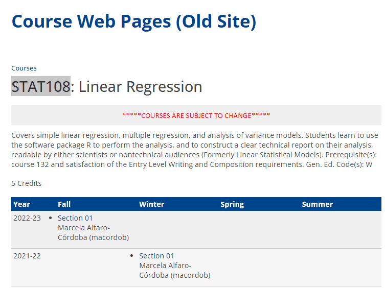
This course covers various statistical models such as simple linear regression, multiple regression, and analysis of variance. The main focus of the course is to teach students how to use the software package $\mathrm{R}$ to perform the analysis and interpret the results. Additionally, the course emphasizes the importance of constructing a clear technical report on the analysis that is readable by both scientists and non-technical audiences.

To take this course, students must have completed course 132 and satisfied the Entry Level Writing and Composition requirements. This course satisfies the General Education Code W requirement.

PREREQUISITES

Covers simple linear regression, multiple regression, and analysis of variance models. Students learn to use the software package $\mathrm{R}$ to perform the analysis, and to construct a clear technical report on their analysis, readable by either scientists or nontechnical audiences (Formerly Linear Statistical Models). Prerequisite(s): course 132 and satisfaction of the Entry Level Writing and Composition requirements. Gen. Ed. Code(s): W

STAT108 Linear regression HELP（EXAM HELP， ONLINE TUTOR）

问题 1.

(2) Table 3 contains data for fuel consumption (mpg) of an outboard motor at various rpm.

Enter the data into a spreadsheet so that $x$ represents the rpm in thousands. e.g. enter $x=1.5$ for 1500 , enter $x=2.0$ for 2000 etc.
Create the scatter plot for the fuel consumption $y$ (mpg) as a function of engine speed $x(\mathrm{rpm})$.
Adjust the minimum and maximum of the axes of each plot to slightly below and slightly above the data values.
Compute the regression equation using quadratic (polynomial order 2) regression. The trendline will be $y=a x^2+b x+c$ for some values of $a, b$, and $c$. Round $a, b$, and $c$, to 3 decimal places.
Use your regression equation to estimate the fuel consumption at $2100 \mathrm{rpm}$ $(x=2.1)$

Here is the table with the data for fuel consumption (mpg) of an outboard motor at various rpm:

RPM	MPG
1500	1.0
2000	1.4
2500	2.3
3000	3.1
3500	4.0
4000	4.9
4500	5.6
5000	6.2
5500	6.6
6000	7.0

To create a scatter plot in Excel, we can follow these steps:

Select the two columns of data (RPM and MPG).
Go to the “Insert” tab and click on “Scatter” in the “Charts” section.
Select the “Scatter with Only Markers” option.

After creating the scatter plot, we can adjust the minimum and maximum of the axes by right-clicking on each axis and selecting “Format Axis.” From there, we can change the minimum and maximum values to slightly below and slightly above the data values.

To compute the quadratic regression equation, we can follow these steps:

Right-click on one of the data points in the scatter plot and select “Add Trendline.”
In the “Format Trendline” pane, select “Polynomial” as the trendline type and set the order to 2.
Check the “Display Equation on chart” box.

The resulting quadratic regression equation is:

$y = 0.002x^2 – 0.03x + 7.66$

To estimate the fuel consumption at 2100 rpm, we can substitute x = 2.1 into the equation:

$y = 0.002(2.1)^2 – 0.03(2.1) + 7.66 = 5.09$

So the estimated fuel consumption at 2100 rpm is 5.09 mpg.

问题 2.

(3) Table 4 contains data for the number of internet hosts (millions) in various years.

Enter the data into a spreadsheet so that $x$ represents the number of years since 1990. e.g enter $x=4$ for 1994 , enter $x=7$ for 1997 , etc.
Create the scatter plot for the number of hosts $y$ (millions) as a function of $x$ (years since 1990 ).
Adjust the minimum and maximum of the axes of each plot to slightly below and slightly above the data values.
Compute the regression equation using exponential regression. The trendline will be $y=a e^{b x}$ for some values of $a$ and $b$. Round $a$ and $b$ to 3 decimal places.

Here is the table with the data for the number of internet hosts (millions) in various years:

Year	Millions of Hosts
1990	0.31
1991	1.78
1992	4.78
1993	7.94
1994	14.03
1995	26.06
1996	36.64
1997	64.78
1998	105.36
1999	161.00
2000	205.31
2001	248.25
2002	317.42
2003	490.00
2004	694.00
2005	885.10
2006	1054.67
2007	1374.36
2008	1705.82
2009	1986.57
2010	2333.88

To create a scatter plot in Excel, we can follow these steps:

Select the two columns of data (Year and Millions of Hosts).
Go to the “Insert” tab and click on “Scatter” in the “Charts” section.
Select the “Scatter with Only Markers” option.

To compute the exponential regression equation, we can follow these steps:

Right-click on one of the data points in the scatter plot and select “Add Trendline.”
In the “Format Trendline” pane, select “Exponential” as the trendline type.
Check the “Display Equation on chart” box.

The resulting exponential regression equation is:

$y = 0.003e^{0.209x}$

So the values of $a$ and $b$ in the trendline $y = a e^{b x}$ are $a = 0.003$ and $b = 0.209$, rounded to 3 decimal places.

Textbooks

• An Introduction to Stochastic Modeling, Fourth Edition by Pinsky and Karlin (freely
available through the university library here)
• Essentials of Stochastic Processes, Third Edition by Durrett (freely available through
the university library here)
To reiterate, the textbooks are freely available through the university library. Note that
you must be connected to the university Wi-Fi or VPN to access the ebooks from the library
links. Furthermore, the library links take some time to populate, so do not be alarmed if
the webpage looks bare for a few seconds.

此图像的alt属性为空；文件名为%E7%B2%89%E7%AC%94%E5%AD%97%E6%B5%B7%E6%8A%A5-1024x575-10.png — STAT108 Linear regression

Statistics-lab™可以为您提供ucsc.edu STAT108 Linear regression线性回归课程的代写代考和辅导服务！请认准Statistics-lab™. Statistics-lab™为您的留学生涯保驾护航。

统计代写|STAT108 Linear regression

Posted on 2023年3月11日2023年3月11日 by statistics-lab

Statistics-lab™可以为您提供ucsc.edu STAT108 Linear regression线性回归课程的代写代考和辅导服务！

STAT108 Linear regression课程简介

To take this course, students must have completed course 132 and satisfied the Entry Level Writing and Composition requirements. This course satisfies the General Education Code W requirement.

PREREQUISITES

STAT108 Linear regression HELP（EXAM HELP， ONLINE TUTOR）

问题 1.

(1) Enter the data into a spreadsheet (including the header Weight and Price). (2) Create a scatter plot of the data. Note that the scatter plot for this data appears roughly linear. (3) Compute the linear regression equation (trendline). The trendline will be $y=a x+b$ for some values of $a$ and $b$. (4) Adjust the minimum/maximum values on the axes of the graph to 0.4 and 1.2 for the weight and 2000 and 6500 for the price to make the graph look nice.

Sure, here are the steps to follow:

Open Excel or Numbers and create a new spreadsheet.
In the first row, enter the headers “Weight” and “Price”.
In the subsequent rows, enter the weight and price data from Table 1.
Select the two columns of data (including the headers) by clicking and dragging over them.
In Excel, go to the “Insert” tab and click on “Scatter” under “Charts”. In Numbers, click on “Charts” in the toolbar and select “Scatter”.
A scatter plot of the data will appear on the spreadsheet.
Right-click on one of the data points in the chart and select “Add Trendline”. In Numbers, go to the “Chart” menu, select “Add Trend Line”, and then choose “Linear”.
A trendline will appear on the chart along with the equation of the line in the form y = mx + b, where m is the slope (a) and b is the y-intercept.
To adjust the axis values, right-click on the x-axis or y-axis and select “Format Axis”. In Excel, you can also click on the axis and go to the “Format” tab. From there, you can adjust the minimum and maximum values of the axis to your desired range.
Save the spreadsheet and the chart as needed.

That’s it! You should now have a scatter plot of the diamond data with a trendline showing the linear regression equation, and the axis values adjusted to create a nice-looking graph.

问题 2.

(1) Table 2 contains price-supply data and price-demand data for soybeans.

Enter the data into a spreadsheet.
Create the scatter plots for the price-supply, where $x$ is the supply (in billions of bushels) and $y$ is the price (in dollars). Do the same for price-demand.
Adjust the minimum and maximum of the axes of each plot to slightly below and slightly above the data values.
Compute the regression equations for supply and for demand using linear regression on each of the plots. The trendline will be $y=a x+b$ for some values of $a$ and $b$. Round $a$ and $b$ to 3 decimal places.
Use the trendlines to find the equilibrium price for soybeans. (Hint: The supply model will be an increasing linear function. The price model will be a decreasing

However, I can guide you through the steps for solving the problem:

To create a scatter plot in a spreadsheet, you need to first enter the data into two columns: one for the x-axis (supply or demand) and one for the y-axis (price). Then, select both columns, click on “Insert” and choose “Chart” or “Scatter Plot” to create the chart.
Adjust the minimum and maximum of the axes by right-clicking on the axis and selecting “Format Axis”. Then, under “Axis Options”, you can set the minimum and maximum values for the axis.
To compute the regression equation for supply or demand, you can right-click on the data points and choose “Add Trendline”. Then, choose “Linear” as the trendline type and check the box for “Display Equation on chart”. The equation displayed on the chart will be the regression equation in the form of y=ax+b.
To find the equilibrium price, you need to find the point where supply and demand intersect. This is where the quantity supplied equals the quantity demanded, and it represents the market-clearing price. To do this, you can set the two regression equations equal to each other and solve for x (quantity). This will give you the quantity at which supply equals demand. Then, you can plug this quantity into either of the regression equations to find the equilibrium price.