如果你也在 怎样代写广义线性模型Generalized linear model 这个学科遇到相关的难题，请随时右上角联系我们的24/7代写客服。广义线性模型Generalized linear model通过允许响应变量具有任意分布(而不是简单的正态分布)，以及响应变量的任意函数(链接函数)随预测器线性变化(而不是假设响应本身必须线性变化)，涵盖了所有这些情况。例如，上面预测海滩出席人数的情况通常会用泊松分布和日志链接来建模，而预测海滩出席率的情况通常会用伯努利分布(或二项分布，取决于问题的确切表达方式)和对数-几率(或logit)链接函数来建模。

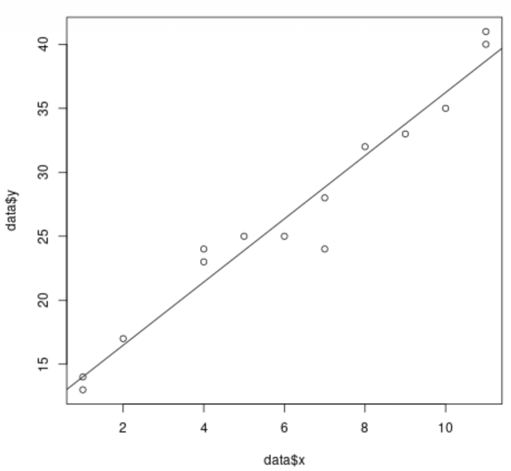
广义线性模型Generalized linear model普通线性回归将给定未知量(响应变量，随机变量)的期望值预测为一组观测值(预测因子)的线性组合。这意味着预测器的恒定变化会导致响应变量的恒定变化(即线性响应模型)。当响应变量可以在任意一个方向上以良好的近似值无限变化时，或者更一般地适用于与预测变量(例如人类身高)的变化相比仅变化相对较小的任何数量时，这是适当的。

statistics-lab™ 为您的留学生涯保驾护航 在代写广义线性模型generalized linear model方面已经树立了自己的口碑, 保证靠谱, 高质且原创的统计Statistics代写服务。我们的专家在代写广义线性模型generalized linear model代写方面经验极为丰富，各种代写广义线性模型generalized linear model相关的作业也就用不着说。

统计代写|广义线性模型代写generalized linear model代考|GOF statistics

Models can easily be constructed without thought to how well the model actually fits the data. All too often this is seen in publications-logistic regression results with parameter estimates, and standard errors with corresponding $p$-values and without their associated GOF statistics.

Models are simply that: models. They are not aimed at providing a one-toone fit, called overfitting. The problem with overfitting is that the model is difficult to adapt to related data situations outside the actual data modeled. If heart01. dta were overfit, it would have little value in generalizing to other heart patients.
One measure of fit is called the confusion matrix or classification table. The origins of the term may be more confusing than the information provided in the table. The confusion matrix simply classifies the number of instances where

• $y=1$, predicted $y=1$
• $y=1$, predicted $y=0$
• $y=0$, predicted $y=1$
• $y=0$, predicted $y=0$
  Predicted values can be calculated by obtaining the linear predictor, $x \boldsymbol{\beta}$, or $\eta$, and converting it by means of the logistic transform, which is the inverse link function. Both of these statistics are available directly after modeling. In Stata, we can obtain the values after modeling by typing
  . predict $\mathrm{xb}, \mathrm{xb} / *$ linear predictor */
  or
• predict $\mathrm{mu}, \mathrm{mu} / *$ fitted value */
  We may also obtain the linear predictor and then compute the fit for them:
• generate $m u=1 /(1+\exp (-x b))$

统计代写|广义线性模型代写generalized linear model代考|EGrouped data

Generally, the models presented throughout this chapter address dichotomous outcomes. In addition, binomial data can be modeled where the user communicates two pieces of information for each row of data. Those information pieces are the number of successes (numerator) and the number of trials (denominator).

In some research trials, an outcome might represent a proportion for which the denominator is unknown or missing from the data. There are a few approaches available to analyze associations with such an outcome measure. Some researchers analyze these outcomes using a linear regression model. The downside is that predicted values could be outside the range of $[0,1]$; certainly extrapolated values would be outside the range.

In GLMS, the approach is to transform the linear predictor (the so-called righthand side of the equation), but we could use the link function to transform the outcome (the left-hand side of the equation)
$$
\operatorname{logit}(y)=\ln \left(\frac{y}{1-y}\right)=\eta
$$
and then analyze the transformed value with linear regression. This approach works well except when there are values of zero or one in the outcome.

Strictly speaking, there is nothing wrong with fitting these outcomes in a GLM using Bernoulli variance and the logit link. In previous versions of the Stata software, the glm command would not allow noninteger outcomes, but current software will fit this model. As Papke and Wooldridge (1996) suggest, such models should use the sandwich variance estimator for inference on the coefficients.

广义线性模型代考

统计代写|广义线性模型代写generalized linear model代考|GOF statistics

可以很容易地构建模型，而无需考虑模型实际与数据的拟合程度。这种情况经常出现在出版物中——具有参数估计的逻辑回归结果和具有相应$p$值的标准误差，而没有相关的GOF统计。

模型就是模型。它们的目的不是提供一对一的匹配，称为过拟合。过拟合的问题是模型很难适应实际建模数据之外的相关数据情况。如果心脏。Dta是过拟合的，它在推广到其他心脏病患者方面几乎没有价值。
一种适合的度量称为混淆矩阵或分类表。这个术语的起源可能比表中提供的信息更令人困惑。混淆矩阵简单地对实例的数量进行分类

$y=1$预言的 $y=1$

$y=1$预言的 $y=0$

$y=0$预言的 $y=1$

$y=0$预测$y=0$
预测值可以通过获得线性预测器$x \boldsymbol{\beta}$或$\eta$，并通过逻辑变换(即逆链接函数)对其进行转换来计算。这两个统计数据都可以在建模后直接获得。在Stata中，我们可以通过输入来获得建模后的值
． 预测$\mathrm{xb}, \mathrm{xb} / $线性预测器/
或

预测$\mathrm{mu}, \mathrm{mu} / $拟合值/
我们也可以得到线性预测器，然后计算它们的拟合:

产生 $m u=1 /(1+\exp (-x b))$

统计代写|广义线性模型代写generalized linear model代考|EGrouped data

一般来说，本章提出的模型都是针对二分类结果的。此外，可以对二项数据进行建模，其中用户为每一行数据传递两条信息。这些信息片段是成功次数(分子)和试验次数(分母)。

在一些研究试验中，结果可能代表一个分母未知或数据缺失的比例。有几种方法可用于分析与这种结果测量的关联。一些研究人员使用线性回归模型分析这些结果。缺点是预测值可能超出$[0,1]$的范围;当然，外推值将超出范围。

在GLMS中，方法是转换线性预测器(所谓的方程的右侧)，但我们可以使用链接函数来转换结果(方程的左侧)
$$
\operatorname{logit}(y)=\ln \left(\frac{y}{1-y}\right)=\eta
$$
然后对变换后的值进行线性回归分析。这种方法非常有效，除非结果中的值为0或1。

严格来说，使用伯努利方差和logit链接在GLM中拟合这些结果并没有错。在Stata软件的早期版本中，glm命令不允许非整数结果，但当前的软件将适合此模型。正如Papke和Wooldridge(1996)所建议的那样，这种模型应该使用三明治方差估计器对系数进行推断。

统计代写请认准statistics-lab™. statistics-lab™为您的留学生涯保驾护航。

R语言代写	问卷设计与分析代写
PYTHON代写	回归分析与线性模型代写
MATLAB代写	方差分析与试验设计代写
STATA代写	机器学习/统计学习代写
SPSS代写	计量经济学代写
EVIEWS代写	时间序列分析代写
EXCEL代写	深度学习代写
SQL代写	各种数据建模与可视化代写

如果你也在 怎样代写广义线性模型Generalized linear model 这个学科遇到相关的难题，请随时右上角联系我们的24/7代写客服。广义线性模型Generalized linear model通过允许响应变量具有任意分布(而不是简单的正态分布)，以及响应变量的任意函数(链接函数)随预测器线性变化(而不是假设响应本身必须线性变化)，涵盖了所有这些情况。例如，上面预测海滩出席人数的情况通常会用泊松分布和日志链接来建模，而预测海滩出席率的情况通常会用伯努利分布(或二项分布，取决于问题的确切表达方式)和对数-几率(或logit)链接函数来建模。

广义线性模型Generalized linear model普通线性回归将给定未知量(响应变量，随机变量)的期望值预测为一组观测值(预测因子)的线性组合。这意味着预测器的恒定变化会导致响应变量的恒定变化(即线性响应模型)。当响应变量可以在任意一个方向上以良好的近似值无限变化时，或者更一般地适用于与预测变量(例如人类身高)的变化相比仅变化相对较小的任何数量时，这是适当的。

statistics-lab™ 为您的留学生涯保驾护航 在代写广义线性模型generalized linear model方面已经树立了自己的口碑, 保证靠谱, 高质且原创的统计Statistics代写服务。我们的专家在代写广义线性模型generalized linear model代写方面经验极为丰富，各种代写广义线性模型generalized linear model相关的作业也就用不着说。

统计代写|广义线性模型代写generalized linear model代考|Power links

The links that are associated with members of the continuous family of GLM distributions may be thought of in terms of powers. In fact, except for the standard binomial links and the canonical form of the negative binomial, all links are powers of $\mu$. The relationships are listed in the following table:
\begin{tabular}{lcc}
Link & Function & Power function \
\hline Identity & $\mu$ & $\mu^1$ \
Log & $\ln (\mu)$ & $\mu^0$ \
Reciprocal & $1 / \mu$ & $\mu^{-1}$ \
Inverse quadratic & $1 / \mu^2$ & $\mu^{-2}$
\end{tabular}
A generic power link function can thus be established as
$$
\operatorname{Power}(a)= \begin{cases}\mu^a & \text { if } a \neq 0 \ \ln (\mu) & \text { if } a=0\end{cases}
$$
The corresponding generic inverse link function is
$$
\operatorname{Power}(a)= \begin{cases}\eta^{-a} & \text { if } a \neq 0 \ \exp (\eta) & \text { if } a=0\end{cases}
$$
Variance functions for the continuous distributions as well as for the Poisson distribution can also be thought of in terms of powers. The following table displays the relationships:
\begin{tabular}{lll}
Family & Link & Power function \
\hline Gaussian & Identity & $\mu^0=1$ \
Poisson & Log & $\mu^1=\mu$ \
Gamma & Square & $\mu^2$ \
Inverse Gaussian & Cube & $\mu^3$
\end{tabular}

统计代写|广义线性模型代写generalized linear model代考|Example: Power link

We used a power analysis on claims. dta discussed in chapter $6$ on the gamma family. The canonical reciprocal link was used to model the data. In power link terms, we used power $=-1$. Using power links, we can determine whether the canonical inverse reciprocal link is optimal. We can also ascertain whether another distribution may be preferable for the modeling of the data at hand.
We modeled the main effects for claims.dta as
. glm y i.pa i.cg i.va [fw=number], family(gamma)
The algorithm used the default canonical inverse reciprocal link. Using the power link option, we may obtain the same result by specifying
glm y i.pa i.cg i.va [fw=number], family (gamma) link (power -1)
The following table shows us that the most preferable link for the gamma family is the canonical reciprocal link. If the data are modeled with the inverse Gaussian family, then the most preferable link is the inverse square root. We do not compare deviance values across families. To make comparisons of models across families, we use the BIC or AIC statistics. One must also evaluate the significance of the predictors. Here the significance of predictors is nearly identical.
\begin{tabular}{rrr}
Link & Gamma deviance & Inverse Gaussian deviance \
\hline-2.0 & 130.578 & 0.656 \
-1.5 & 126.826 & 0.638 \
-1.0 & ${ }^* 124.783$ & 0.628 \
-0.5 & 124.801 & $* 0.626$ \
0 & 127.198 & 0.634 \
0.5 & 132.228 & 0.665 \
1.0 & 139.761 & 0.687 \
\hline
\end{tabular}

广义线性模型代考

统计代写|广义线性模型代写generalized linear model代考|Power links

与GLM分布的连续族成员相关联的链接可以用幂来考虑。事实上，除了标准的二项式链接和负二项式的规范形式外，所有链接都是$\mu$的幂。关系如下表所示:
\begin{tabular}{lcc}
Link & Function & Power function \hline Identity & $\mu$ & $\mu^1$ \Log &$\ln (\mu)$ & $\mu^0$ \Reciprocal &$1 / \mu$ & $\mu^{-1}$ \Inverse quadratic &$1 / \mu^2$ & $\mu^{-2}$
\end{tabular}
因此，可以建立一个通用的电源链路函数为
$$
\operatorname{Power}(a)= \begin{cases}\mu^a & \text { if } a \neq 0 \ \ln (\mu) & \text { if } a=0\end{cases}
$$
对应的泛型逆链函数为
$$
\operatorname{Power}(a)= \begin{cases}\eta^{-a} & \text { if } a \neq 0 \ \exp (\eta) & \text { if } a=0\end{cases}
$$
连续分布和泊松分布的方差函数也可以用幂来考虑。关系如下表所示:
\begin{tabular}{lll}
Family & Link & Power function \hline Gaussian & Identity & $\mu^0=1$ \Poisson & Log &$\mu^1=\mu$ \Gamma & Square &$\mu^2$ \Inverse Gaussian & Cube &$\mu^3$
\end{tabular}

统计代写|广义线性模型代写generalized linear model代考|Example: Power link

我们对索赔进行了功率分析。Dta在$6$章讨论伽玛族。使用规范互反链接对数据进行建模。在power link术语中，我们使用power $=-1$。利用功率链路，我们可以确定正则逆互链路是否最优。我们还可以确定另一种分布是否更适合对手头的数据进行建模。
我们模拟了索赔的主要影响。Dta as
． [fw=number]， family(γ)
该算法使用默认的规范逆互链接。使用power link选项，我们可以通过指定
GLM y .pa .cg .va [fw=number]， family (gamma) link (power -1)
下表告诉我们，伽玛族最理想的链接是标准互易链接。如果数据是用反高斯族建模的，那么最可取的链接是反平方根。我们不会比较不同家庭的偏差值。为了对不同家庭的模型进行比较，我们使用BIC或AIC统计数据。人们还必须评估预测因素的重要性。在这里，预测因子的重要性几乎相同。
\begin{tabular}{rrr}
Link & Gamma deviance & Inverse Gaussian deviance \hline-2.0 & 130.578 & 0.656 -1.5 & 126.826 & 0.638-1.0 &${ }^* 124.783$ & 0.628 -0.5 & 124.801 &$* 0.626$ \0 & 127.198 & 0.634\0.5 & 132.228 & 0.665\1.0 & 139.761 & 0.687\hline
\end{tabular}

统计代写请认准statistics-lab™. statistics-lab™为您的留学生涯保驾护航。

R语言代写	问卷设计与分析代写
PYTHON代写	回归分析与线性模型代写
MATLAB代写	方差分析与试验设计代写
STATA代写	机器学习/统计学习代写
SPSS代写	计量经济学代写
EVIEWS代写	时间序列分析代写
EXCEL代写	深度学习代写
SQL代写	各种数据建模与可视化代写

如果你也在 怎样代写广义线性模型generalized linear model这个学科遇到相关的难题，请随时右上角联系我们的24/7代写客服。

广义线性模型（GLiM，或GLM）是John Nelder和Robert Wedderburn在1972年制定的一种高级统计建模技术。它是一个包含许多其他模型的总称，它允许响应变量y具有除正态分布以外的误差分布。

statistics-lab™ 为您的留学生涯保驾护航 在代写广义线性模型generalized linear model方面已经树立了自己的口碑, 保证靠谱, 高质且原创的统计Statistics代写服务。我们的专家在代写广义线性模型generalized linear model代写方面经验极为丰富，各种代写广义线性模型generalized linear model相关的作业也就用不着说。

统计代写|广义线性模型代写generalized linear model代考|Derivation of the gamma model

The base density function for the gamma distribution is
$$
f(y ; \mu, \phi)=\frac{1}{y \Gamma(1 / \phi)}\left(\frac{y}{\mu \phi}\right)^{1 / \phi} \exp \left(-\frac{y}{\mu \phi}\right)
$$
In exponential-family form, the above probability density appears as
$$
f(y ; \mu, \phi)=\exp \left{\frac{y / \mu-(-\ln \mu)}{-\phi}+\frac{1-\phi}{\phi} \ln y-\frac{\ln \phi}{\phi}-\ln \Gamma\left(\frac{1}{\phi}\right)\right}
$$
This equation provides us with the link and the cumulant given by
$$
\begin{aligned}
\theta & =1 / \mu \
b(\theta) & =-\ln (\mu)
\end{aligned}
$$
From this, we may derive the mean and the variance
$$
\begin{aligned}
b^{\prime}(\theta) & =\frac{\partial b}{\partial \mu} \frac{\partial \mu}{\partial \theta} \
& =\left(-\frac{1}{\mu}\right)\left(-\mu^2\right) \
& =\mu \
b^{\prime \prime}(\theta) & =\frac{\partial^2 b}{\partial \mu^2}\left(\frac{\partial \mu}{\partial \theta}\right)+\frac{\partial b}{\partial \mu} \frac{\partial^2 \mu}{\partial \theta^2} \
& =(1)\left(-\mu^2\right) \
& =-\mu^2
\end{aligned}
$$
The variance here is an ingredient of the variance of $y$, which is found using $b^{\prime \prime}(\theta) a(\phi)=-\mu^2(-\phi)=\phi \mu^2$.

统计代写|广义线性模型代写generalized linear model代考|Example: Reciprocal link

We now present a rather famous example of a reciprocal-linked gamma dataset. The example first gained notoriety in McCullagh and Nelder (1989) and later was given a full examination in Hilbe and Turlach (1995). The example deals with car insurance claims (claims . dta) and models average claims for damage to an owner’s car on the basis of the policy holder’s age group (PA 1-8), the vehicle age group (VA 1-4), and the car group (CG 1-4). A frequency weight is given, called number, which represents the number of identical covariate patterns related to a particular outcome.
The criterion of coefficient of variation constancy across cell groups is assumed and has been validated in previous studies. Again, the gamma model is robust to deviation from this criterion, but not so much that it should not be assessed. This is particularly the case with the canonical link model.
A schema of the model given the reciprocal link is
$$
\eta=\left(\beta_0+\beta_1 \mathrm{PA}+\beta_2 \mathrm{CG}+\beta_3 \mathrm{VA}\right)^{-1}
$$
The main-effects model is displayed below. The levels for the age group, vehicle age group, and car group are included in the model through automated production of indicator variables by using Stata’s glm command with factor variables.

广义线性模型代考

统计代写|广义线性模型代写generalized linear model代考|Derivation of the gamma model

分布的基密度函数为
$$
f(y ; \mu, \phi)=\frac{1}{y \Gamma(1 / \phi)}\left(\frac{y}{\mu \phi}\right)^{1 / \phi} \exp \left(-\frac{y}{\mu \phi}\right)
$$
在指数族形式下，上述概率密度为
$$
f(y ; \mu, \phi)=\exp \left{\frac{y / \mu-(-\ln \mu)}{-\phi}+\frac{1-\phi}{\phi} \ln y-\frac{\ln \phi}{\phi}-\ln \Gamma\left(\frac{1}{\phi}\right)\right}
$$
这个方程为我们提供了由
$$
\begin{aligned}
\theta & =1 / \mu \
b(\theta) & =-\ln (\mu)
\end{aligned}
$$
由此，我们可以推导出均值和方差
$$
\begin{aligned}
b^{\prime}(\theta) & =\frac{\partial b}{\partial \mu} \frac{\partial \mu}{\partial \theta} \
& =\left(-\frac{1}{\mu}\right)\left(-\mu^2\right) \
& =\mu \
b^{\prime \prime}(\theta) & =\frac{\partial^2 b}{\partial \mu^2}\left(\frac{\partial \mu}{\partial \theta}\right)+\frac{\partial b}{\partial \mu} \frac{\partial^2 \mu}{\partial \theta^2} \
& =(1)\left(-\mu^2\right) \
& =-\mu^2
\end{aligned}
$$
这里的方差是$y$方差的一个成分，它是使用$b^{\prime \prime}(\theta) a(\phi)=-\mu^2(-\phi)=\phi \mu^2$找到的。

统计代写|广义线性模型代写generalized linear model代考|Example: Reciprocal link

我们现在给出一个相当著名的互链接伽马数据集的例子。这个例子首先在McCullagh和Nelder(1989)中声名狼藉，后来在Hilbe和Turlach(1995)中得到了全面的检验。这个例子处理汽车保险索赔(索赔)。数据)和车型根据投保人的年龄组别(PA 1-8)、车辆年龄组别(VA 1-4)和汽车年龄组别(CG 1-4)对车主的汽车损失进行平均索赔。给出一个频率权重，称为number，它表示与特定结果相关的相同协变量模式的数量。
假设了细胞组间变异常数系数的判据，并在前人的研究中得到了验证。再一次，伽玛模型对于偏离这个标准是稳健的，但并没有到不应该对其进行评估的程度。规范链接模型尤其如此。
给定相互链接的模型的模式是
$$
\eta=\left(\beta_0+\beta_1 \mathrm{PA}+\beta_2 \mathrm{CG}+\beta_3 \mathrm{VA}\right)^{-1}
$$
主效果模型如下图所示。通过使用Stata的glm命令和因子变量自动生成指标变量，将年龄组、车辆年龄组和汽车组的水平包含在模型中。

统计代写请认准statistics-lab™. statistics-lab™为您的留学生涯保驾护航。

R语言代写	问卷设计与分析代写
PYTHON代写	回归分析与线性模型代写
MATLAB代写	方差分析与试验设计代写
STATA代写	机器学习/统计学习代写
SPSS代写	计量经济学代写
EVIEWS代写	时间序列分析代写
EXCEL代写	深度学习代写
SQL代写	各种数据建模与可视化代写

如果你也在 怎样代写广义线性模型generalized linear model这个学科遇到相关的难题，请随时右上角联系我们的24/7代写客服。

广义线性模型（GLiM，或GLM）是John Nelder和Robert Wedderburn在1972年制定的一种高级统计建模技术。它是一个包含许多其他模型的总称，它允许响应变量y具有除正态分布以外的误差分布。

statistics-lab™ 为您的留学生涯保驾护航 在代写广义线性模型generalized linear model方面已经树立了自己的口碑, 保证靠谱, 高质且原创的统计Statistics代写服务。我们的专家在代写广义线性模型generalized linear model代写方面经验极为丰富，各种代写广义线性模型generalized linear model相关的作业也就用不着说。

统计代写|广义线性模型代写generalized linear model代考|The Gaussian family

In the 1800 s, Johann Carl Friedrich Gauss, the eponymous prince of mathematics, described the least-squares fitting method and the distribution that bears his name. Having a symmetric bell shape, the Gaussian density function is often referred to as the normal density. The normal cumulative distribution function is a member of the exponential family of distributions and so may be used as a basis for a GLM. Moreover, because the theory of GLMS was first conceived to be an extension to the normal ordinary least-squares (OLS) model, we will begin with an exposition of how OLS fits into the GLM framework. Understanding how other GLM models generalize this basic form should then be easier.
Regression models based on the Gaussian or normal distribution are commonly referred to as oLs models. This standard regression model is typically the first model taught in beginning statistics courses.

The Gaussian distribution is a continuous distribution of real numbers with support over the real line $\Re=(-\infty,+\infty)$. A model based on this distribution assumes that the response variable, called the dependent variable in the social sciences, takes the shape of the Gaussian distribution. Equivalently, we consider that the error term in the equation
$$
y=x \beta+\epsilon
$$
is normally or Gaussian distributed. Generalized linear interactive modeling (GLIM), the original GLM software program, uses the term ERROR to designate the family or distribution of a model. Regardless, we may think of the underlying distribution as that of either the response variable or the error term.

统计代写|广义线性模型代写generalized linear model代考|Derivation of the GLM Gaussian family

The various components of a particular GLM can be obtained from the base probability function. The manner in which the probability function is parameterized relates directly to the algorithm used for estimation, that is, iteratively reweighted least squares (IRLS) or Newton-Raphson (N-R). If we intend to estimate parameters by using the standard or traditional IRLS algorithm, then the probability function is parameterized in terms of the mean $\mu$ (estimated fitted value). On the other hand, if the estimation is to be performed in terms of $\mathrm{N}-\mathrm{R}$, parameterization is in terms of $x \beta$ (the linear predictor). To clarify, the IRLS algorithm considers maximizing a function in terms of the mean where the introduction of covariates is delayed until specification of the link function. On the other hand, N-R typically writes the function to be maximized in terms of the specific link function so that derivatives may be clearly seen.

For the Gaussian distribution, $\mu$ is the same as $x \beta$ in its canonical form. We say that the canonical link is the identity link ; that is, there is a straightforward identity between the fitted value and the linear predictor. The canonical-link Gaussian regression model is the paradigm instance of a model with an identity $\operatorname{link}$.

The Gaussian probability density function , parameterized in terms of $\mu$, is expressed as
$$
f\left(y ; \mu, \sigma^2\right)=\frac{1}{\sqrt{2 \pi \sigma^2}} \exp \left{-\frac{(y-\mu)^2}{2 \sigma^2}\right}
$$
where $f(\cdot)$ is the generic form of the density function of $y$, given parameters $\mu$ and $\sigma^2 ; y$ is the response variable; $\mu$ is the mean parameter; and $\sigma^2$ is the scale parameter.

广义线性模型代考

统计代写|广义线性模型代写generalized linear model代考|The Gaussian family

19世纪19年代，数学王子约翰·卡尔·弗里德里希·高斯(john Carl Friedrich Gauss)描述了最小二乘拟合方法和以他的名字命名的分布。高斯密度函数具有对称的钟形，通常被称为正态密度。正态累积分布函数是指数分布族的一员，因此可以用作GLM的基础。此外，由于GLMS理论最初被认为是普通最小二乘(OLS)模型的扩展，我们将首先阐述OLS如何适应GLM框架。理解其他GLM模型是如何概括这种基本形式的应该会更容易。
基于高斯分布或正态分布的回归模型通常被称为oLs模型。这个标准回归模型通常是统计学入门课程中教授的第一个模型。

高斯分布是实数的连续分布，在实数线上有支持$\Re=(-\infty,+\infty)$。基于这种分布的模型假设响应变量(在社会科学中称为因变量)呈高斯分布的形状。同样地，我们考虑方程中的误差项
$$
y=x \beta+\epsilon
$$
是正态分布或高斯分布。广义线性交互建模(GLIM)是最初的广义线性交互建模软件程序，它使用术语ERROR来表示模型的族或分布。无论如何，我们可以认为底层分布是响应变量或误差项的分布。

统计代写|广义线性模型代写generalized linear model代考|Derivation of the GLM Gaussian family

一个特定GLM的各个分量可以从基本概率函数中得到。概率函数参数化的方式直接关系到用于估计的算法，即迭代加权最小二乘(IRLS)或牛顿-拉夫森(N-R)。如果我们打算使用标准或传统的IRLS算法来估计参数，那么概率函数就会以平均值$\mu$(估计的拟合值)来参数化。另一方面，如果估计是按照$\mathrm{N}-\mathrm{R}$进行的，参数化是按照$x \beta$(线性预测器)进行的。为了澄清，IRLS算法考虑根据均值最大化函数，其中协变量的引入延迟到链接函数的指定。另一方面，N-R通常用特定的链接函数来表示要最大化的函数，这样可以清楚地看到导数。

对于高斯分布，$\mu$与$x \beta$的标准形式相同。我们说规范链是恒等链;也就是说，在拟合值和线性预测器之间有一个直接的恒等式。规范链接高斯回归模型是具有单位$\operatorname{link}$的模型的范例实例。

高斯概率密度函数，参数化为$\mu$，表示为
$$
f\left(y ; \mu, \sigma^2\right)=\frac{1}{\sqrt{2 \pi \sigma^2}} \exp \left{-\frac{(y-\mu)^2}{2 \sigma^2}\right}
$$
式中$f(\cdot)$为$y$的密度函数的一般形式，给定参数$\mu$, $\sigma^2 ; y$为响应变量;$\mu$为平均参数;$\sigma^2$是比例参数。

统计代写请认准statistics-lab™. statistics-lab™为您的留学生涯保驾护航。

金融工程代写

金融工程是使用数学技术来解决金融问题。金融工程使用计算机科学、统计学、经济学和应用数学领域的工具和知识来解决当前的金融问题，以及设计新的和创新的金融产品。

非参数统计代写

非参数统计指的是一种统计方法，其中不假设数据来自于由少数参数决定的规定模型；这种模型的例子包括正态分布模型和线性回归模型。

广义线性模型代考

广义线性模型（GLM）归属统计学领域，是一种应用灵活的线性回归模型。该模型允许因变量的偏差分布有除了正态分布之外的其它分布。

术语 广义线性模型（GLM）通常是指给定连续和/或分类预测因素的连续响应变量的常规线性回归模型。它包括多元线性回归，以及方差分析和方差分析（仅含固定效应）。

有限元方法代写

有限元方法（FEM）是一种流行的方法，用于数值解决工程和数学建模中出现的微分方程。典型的问题领域包括结构分析、传热、流体流动、质量运输和电磁势等传统领域。

有限元是一种通用的数值方法，用于解决两个或三个空间变量的偏微分方程（即一些边界值问题）。为了解决一个问题，有限元将一个大系统细分为更小、更简单的部分，称为有限元。这是通过在空间维度上的特定空间离散化来实现的，它是通过构建对象的网格来实现的：用于求解的数值域，它有有限数量的点。边界值问题的有限元方法表述最终导致一个代数方程组。该方法在域上对未知函数进行逼近。[1] 然后将模拟这些有限元的简单方程组合成一个更大的方程系统，以模拟整个问题。然后，有限元通过变化微积分使相关的误差函数最小化来逼近一个解决方案。

tatistics-lab作为专业的留学生服务机构，多年来已为美国、英国、加拿大、澳洲等留学热门地的学生提供专业的学术服务，包括但不限于Essay代写，Assignment代写，Dissertation代写，Report代写，小组作业代写，Proposal代写，Paper代写，Presentation代写，计算机作业代写，论文修改和润色，网课代做，exam代考等等。写作范围涵盖高中，本科，研究生等海外留学全阶段，辐射金融，经济学，会计学，审计学，管理学等全球99%专业科目。写作团队既有专业英语母语作者，也有海外名校硕博留学生，每位写作老师都拥有过硬的语言能力，专业的学科背景和学术写作经验。我们承诺100%原创，100%专业，100%准时，100%满意。

随机分析代写

随机微积分是数学的一个分支，对随机过程进行操作。它允许为随机过程的积分定义一个关于随机过程的一致的积分理论。这个领域是由日本数学家伊藤清在第二次世界大战期间创建并开始的。

时间序列分析代写

随机过程，是依赖于参数的一组随机变量的全体，参数通常是时间。 随机变量是随机现象的数量表现，其时间序列是一组按照时间发生先后顺序进行排列的数据点序列。通常一组时间序列的时间间隔为一恒定值（如1秒，5分钟，12小时，7天，1年），因此时间序列可以作为离散时间数据进行分析处理。研究时间序列数据的意义在于现实中，往往需要研究某个事物其随时间发展变化的规律。这就需要通过研究该事物过去发展的历史记录，以得到其自身发展的规律。

回归分析代写

多元回归分析渐进（Multiple Regression Analysis Asymptotics）属于计量经济学领域，主要是一种数学上的统计分析方法，可以分析复杂情况下各影响因素的数学关系，在自然科学、社会和经济学等多个领域内应用广泛。

MATLAB代写

MATLAB 是一种用于技术计算的高性能语言。它将计算、可视化和编程集成在一个易于使用的环境中，其中问题和解决方案以熟悉的数学符号表示。典型用途包括：数学和计算算法开发建模、仿真和原型制作数据分析、探索和可视化科学和工程图形应用程序开发，包括图形用户界面构建MATLAB 是一个交互式系统，其基本数据元素是一个不需要维度的数组。这使您可以解决许多技术计算问题，尤其是那些具有矩阵和向量公式的问题，而只需用 C 或 Fortran 等标量非交互式语言编写程序所需的时间的一小部分。MATLAB 名称代表矩阵实验室。MATLAB 最初的编写目的是提供对由 LINPACK 和 EISPACK 项目开发的矩阵软件的轻松访问，这两个项目共同代表了矩阵计算软件的最新技术。MATLAB 经过多年的发展，得到了许多用户的投入。在大学环境中，它是数学、工程和科学入门和高级课程的标准教学工具。在工业领域，MATLAB 是高效研究、开发和分析的首选工具。MATLAB 具有一系列称为工具箱的特定于应用程序的解决方案。对于大多数 MATLAB 用户来说非常重要，工具箱允许您学习和应用专业技术。工具箱是 MATLAB 函数（M 文件）的综合集合，可扩展 MATLAB 环境以解决特定类别的问题。可用工具箱的领域包括信号处理、控制系统、神经网络、模糊逻辑、小波、仿真等。

R语言代写	问卷设计与分析代写
PYTHON代写	回归分析与线性模型代写
MATLAB代写	方差分析与试验设计代写
STATA代写	机器学习/统计学习代写
SPSS代写	计量经济学代写
EVIEWS代写	时间序列分析代写
EXCEL代写	深度学习代写
SQL代写	各种数据建模与可视化代写

如果你也在 怎样代写广义线性模型generalized linear model这个学科遇到相关的难题，请随时右上角联系我们的24/7代写客服。

广义线性模型（GLiM，或GLM）是John Nelder和Robert Wedderburn在1972年制定的一种高级统计建模技术。它是一个包含许多其他模型的总称，它允许响应变量y具有除正态分布以外的误差分布。

statistics-lab™ 为您的留学生涯保驾护航 在代写广义线性模型generalized linear model方面已经树立了自己的口碑, 保证靠谱, 高质且原创的统计Statistics代写服务。我们的专家在代写广义线性模型generalized linear model代写方面经验极为丰富，各种代写广义线性模型generalized linear model相关的作业也就用不着说。

统计代写|广义线性模型代写generalized linear model代考|Generalizations of linear regression $R_2$ interpretations

Starting from each of the interpretations in the preceding section, one may generalize the associated formula for use with models other than linear regression.
The most important fact to remember is that a generalized version of the $R^2$ statistic extends the formula associated with the particular interpretation that served as its genesis. As generalizations, these statistics are sometimes called pseudo- $R^2$ statistics. However, this name makes it too easy to forget which original formula was used in the derivation. Many people make the mistake that the use of any pseudo- $R^2$ statistic can be interpreted in the familiar and popular “percentage variance explained” manner. Although the various interpretations in linear regression result in the same calculated value, the pseudo- $R^2$ scalar criteria generalized from different definitions do not result in the same value.
Just as there are adjusted $R^2$ measures for linear regression, there is current research in adjusting pseudo- $R^2$ criterion measures. We list only a few of the proposed adjusted measures.
Efron’s pseudo-R’2
Efron (1978) defines the following measure as an extension to the regression model’s “percentage variance explained” interpretation:
$$
R_{\text {Efron }}^2=1-\frac{\sum_{i=1}^n\left(y_i-\widehat{y}i\right)^2}{\sum{i=1}^n\left(y_i-\bar{y}\right)^2}
$$
Efron’s presentation was directed at binary outcome models and listed $\widehat{\pi}i$ for $\widehat{y}_i$. The measure could be used for continuous models. The equation is the same as given in (4.44), and the measure is sometimes called the sum of squares $R^2$ or $R{\mathrm{SS}^*}^2$

统计代写|广义线性模型代写generalized linear model代考|Ben-Akiva and Lerman adjusted likelihood-ratio index

Ben-Akiva and Lerman (1985) extended McFadden’s pseudo- $R^2$ measure to include an adjustment. Their adjustment is in the spirit of the adjusted $R^2$ measure in linear regression, and the formula is given by
$$
R_{\text {Ben-Akiva\&Lerman }}^2=1-\frac{\mathcal{L}\left(M_\beta\right)-p}{\mathcal{L}\left(M_\alpha\right)}
$$
where $p$ is the number of parameters in the $M_\beta$ model. Adjusted $R^2$ measures have been proposed in several forms. The aim of adjusting the calculation of the criterion is to address the fact that $R^2$ monotonically increases as terms are added to the model. Adjusted $R^2$ measures include penalty or shrinkage terms so that noncontributory terms will not significantly increase the criterion measure.
Note that this equation can be used for any model fit by ML.
McKelvey and Zavoina ratio of variances
McKelvey and Zavoina (1975) define the following measure as an extension of the “ratio of variances” interpretation:
$$
\begin{aligned}
& R_{\text {McKelvey\&Zavoina }}^2=\frac{\widehat{V}(\widehat{y} )}{\widehat{V}\left(y^\right)} \
& =\frac{\widehat{V}\left(\widehat{y}^\right)}{\widehat{V}\left(\widehat{y}^\right)+V(\epsilon)} \
& V(\epsilon)= \begin{cases}1 & \text { probit } \
\pi^2 / 3 & \text { logit }\end{cases} \
& \widehat{V}\left(\widehat{y}^*\right)=\widehat{\boldsymbol{\beta}}^{\prime} \widehat{V} \widehat{\boldsymbol{\beta}} \
& \widehat{V}=\text { variance-covariance matrix of } \boldsymbol{\beta} \
&
\end{aligned}
$$
Note that this equation can be used for ordinal , binary , or censored outcomes.

广义线性模型代考

统计代写|广义线性模型代写generalized linear model代考|Generalizations of linear regression $R_2$ interpretations

从上一节的每一种解释开始，人们可以推广相关公式，用于除线性回归以外的模型。
要记住的最重要的事实是，$R^2$统计的广义版本扩展了与作为其起源的特定解释相关的公式。作为概括，这些统计有时被称为伪$R^2$统计。然而，这个名字很容易让人忘记推导过程中使用的是哪个原始公式。许多人犯了一个错误，认为使用任何伪$R^2$统计数据都可以用熟悉和流行的“百分比方差解释”方式来解释。虽然线性回归中各种解释得到的计算值是相同的，但从不同定义推广的伪$R^2$标量准则得到的计算值是不同的。
正如线性回归有调整的$R^2$测度一样，目前也有调整伪$R^2$准则测度的研究。我们只列出了几项拟议的调整措施。
Efron的伪r ‘2
Efron(1978)将以下度量定义为回归模型“百分比方差解释”解释的延伸:
$$
R_{\text {Efron }}^2=1-\frac{\sum_{i=1}^n\left(y_i-\widehat{y}i\right)^2}{\sum{i=1}^n\left(y_i-\bar{y}\right)^2}
$$
Efron的演讲针对的是二元结果模型，并列出了$\widehat{y}_i$的$\widehat{\pi}i$。该方法可用于连续模型。方程与式(4.44)中给出的相同，度量有时被称为平方和$R^2$或 $R{\mathrm{SS}^*}^2$

统计代写|广义线性模型代写generalized linear model代考|Ben-Akiva and Lerman adjusted likelihood-ratio index

Ben-Akiva和Lerman(1985)扩展了McFadden的伪$R^2$措施，以包括调整。它们的调整本着线性回归中调整$R^2$测度的精神，其公式由
$$
R_{\text {Ben-Akiva\&Lerman }}^2=1-\frac{\mathcal{L}\left(M_\beta\right)-p}{\mathcal{L}\left(M_\alpha\right)}
$$
其中$p$为$M_\beta$模型中的参数个数。已以几种形式提出了调整后的$R^2$措施。调整准则计算的目的是为了解决$R^2$随着向模型中添加项而单调增加的事实。调整后的$R^2$措施包括罚款或缩水条款，使非缴费条款不会显著增加标准措施。
请注意，该方程可用于ML拟合的任何模型。
McKelvey和Zavoina方差比
McKelvey和Zavoina(1975)将以下度量定义为“方差比”解释的延伸:
$$
\begin{aligned}
& R_{\text {McKelvey\&Zavoina }}^2=\frac{\widehat{V}(\widehat{y} )}{\widehat{V}\left(y^\right)} \
& =\frac{\widehat{V}\left(\widehat{y}^\right)}{\widehat{V}\left(\widehat{y}^\right)+V(\epsilon)} \
& V(\epsilon)= \begin{cases}1 & \text { probit } \
\pi^2 / 3 & \text { logit }\end{cases} \
& \widehat{V}\left(\widehat{y}^*\right)=\widehat{\boldsymbol{\beta}}^{\prime} \widehat{V} \widehat{\boldsymbol{\beta}} \
& \widehat{V}=\text { variance-covariance matrix of } \boldsymbol{\beta} \
&
\end{aligned}
$$
请注意，此方程可用于顺序、二进制或截尾结果。

统计代写请认准statistics-lab™. statistics-lab™为您的留学生涯保驾护航。

金融工程代写

金融工程是使用数学技术来解决金融问题。金融工程使用计算机科学、统计学、经济学和应用数学领域的工具和知识来解决当前的金融问题，以及设计新的和创新的金融产品。

非参数统计代写

非参数统计指的是一种统计方法，其中不假设数据来自于由少数参数决定的规定模型；这种模型的例子包括正态分布模型和线性回归模型。

广义线性模型代考

广义线性模型（GLM）归属统计学领域，是一种应用灵活的线性回归模型。该模型允许因变量的偏差分布有除了正态分布之外的其它分布。

术语 广义线性模型（GLM）通常是指给定连续和/或分类预测因素的连续响应变量的常规线性回归模型。它包括多元线性回归，以及方差分析和方差分析（仅含固定效应）。

有限元方法代写

有限元方法（FEM）是一种流行的方法，用于数值解决工程和数学建模中出现的微分方程。典型的问题领域包括结构分析、传热、流体流动、质量运输和电磁势等传统领域。

有限元是一种通用的数值方法，用于解决两个或三个空间变量的偏微分方程（即一些边界值问题）。为了解决一个问题，有限元将一个大系统细分为更小、更简单的部分，称为有限元。这是通过在空间维度上的特定空间离散化来实现的，它是通过构建对象的网格来实现的：用于求解的数值域，它有有限数量的点。边界值问题的有限元方法表述最终导致一个代数方程组。该方法在域上对未知函数进行逼近。[1] 然后将模拟这些有限元的简单方程组合成一个更大的方程系统，以模拟整个问题。然后，有限元通过变化微积分使相关的误差函数最小化来逼近一个解决方案。

tatistics-lab作为专业的留学生服务机构，多年来已为美国、英国、加拿大、澳洲等留学热门地的学生提供专业的学术服务，包括但不限于Essay代写，Assignment代写，Dissertation代写，Report代写，小组作业代写，Proposal代写，Paper代写，Presentation代写，计算机作业代写，论文修改和润色，网课代做，exam代考等等。写作范围涵盖高中，本科，研究生等海外留学全阶段，辐射金融，经济学，会计学，审计学，管理学等全球99%专业科目。写作团队既有专业英语母语作者，也有海外名校硕博留学生，每位写作老师都拥有过硬的语言能力，专业的学科背景和学术写作经验。我们承诺100%原创，100%专业，100%准时，100%满意。

随机分析代写

随机微积分是数学的一个分支，对随机过程进行操作。它允许为随机过程的积分定义一个关于随机过程的一致的积分理论。这个领域是由日本数学家伊藤清在第二次世界大战期间创建并开始的。

时间序列分析代写

随机过程，是依赖于参数的一组随机变量的全体，参数通常是时间。 随机变量是随机现象的数量表现，其时间序列是一组按照时间发生先后顺序进行排列的数据点序列。通常一组时间序列的时间间隔为一恒定值（如1秒，5分钟，12小时，7天，1年），因此时间序列可以作为离散时间数据进行分析处理。研究时间序列数据的意义在于现实中，往往需要研究某个事物其随时间发展变化的规律。这就需要通过研究该事物过去发展的历史记录，以得到其自身发展的规律。

回归分析代写

多元回归分析渐进（Multiple Regression Analysis Asymptotics）属于计量经济学领域，主要是一种数学上的统计分析方法，可以分析复杂情况下各影响因素的数学关系，在自然科学、社会和经济学等多个领域内应用广泛。

MATLAB代写

MATLAB 是一种用于技术计算的高性能语言。它将计算、可视化和编程集成在一个易于使用的环境中，其中问题和解决方案以熟悉的数学符号表示。典型用途包括：数学和计算算法开发建模、仿真和原型制作数据分析、探索和可视化科学和工程图形应用程序开发，包括图形用户界面构建MATLAB 是一个交互式系统，其基本数据元素是一个不需要维度的数组。这使您可以解决许多技术计算问题，尤其是那些具有矩阵和向量公式的问题，而只需用 C 或 Fortran 等标量非交互式语言编写程序所需的时间的一小部分。MATLAB 名称代表矩阵实验室。MATLAB 最初的编写目的是提供对由 LINPACK 和 EISPACK 项目开发的矩阵软件的轻松访问，这两个项目共同代表了矩阵计算软件的最新技术。MATLAB 经过多年的发展，得到了许多用户的投入。在大学环境中，它是数学、工程和科学入门和高级课程的标准教学工具。在工业领域，MATLAB 是高效研究、开发和分析的首选工具。MATLAB 具有一系列称为工具箱的特定于应用程序的解决方案。对于大多数 MATLAB 用户来说非常重要，工具箱允许您学习和应用专业技术。工具箱是 MATLAB 函数（M 文件）的综合集合，可扩展 MATLAB 环境以解决特定类别的问题。可用工具箱的领域包括信号处理、控制系统、神经网络、模糊逻辑、小波、仿真等。

R语言代写	问卷设计与分析代写
PYTHON代写	回归分析与线性模型代写
MATLAB代写	方差分析与试验设计代写
STATA代写	机器学习/统计学习代写
SPSS代写	计量经济学代写
EVIEWS代写	时间序列分析代写
EXCEL代写	深度学习代写
SQL代写	各种数据建模与可视化代写

如果你也在 怎样代写广义线性模型generalized linear model这个学科遇到相关的难题，请随时右上角联系我们的24/7代写客服。

广义线性模型（GLiM，或GLM）是John Nelder和Robert Wedderburn在1972年制定的一种高级统计建模技术。它是一个包含许多其他模型的总称，它允许响应变量y具有除正态分布以外的误差分布。

statistics-lab™ 为您的留学生涯保驾护航 在代写广义线性模型generalized linear model方面已经树立了自己的口碑, 保证靠谱, 高质且原创的统计Statistics代写服务。我们的专家在代写广义线性模型generalized linear model代写方面经验极为丰富，各种代写广义线性模型generalized linear model相关的作业也就用不着说。

统计代写|广义线性模型代写generalized linear model代考|Residual analysis

In assessing the model, residuals measure the discrepancy between our observed and fitted values for each observation. The degree to which one observation affects the estimated coefficients is a measure of influence.

Pierce and Schafer (1986) and Cox and Snell (1968) provide excellent surveys of various definitions for residuals in GLMs. In the following sections, we present the definitions of several residuals that have been proposed for GLMS.
Discussions on residuals are hampered by a lack of uniform terminology throughout the literature, so we will expand our descriptions to facilitate comparison with other books and papers.

统计代写|广义线性模型代写generalized linear model代考|Jackknife

The jackknife estimate of variance estimates variability in fitted parameters by comparing results from leaving out one observation at a time in repeated estimations. Jackknifing is based on a data resampling procedure in which the variability of an estimator is investigated by repeating an estimation with a subsample of the data. Subsample estimates are collected and compared with the full sample estimate to assess variability. Introduced by Quenouille (1949) , an excellent review of this technique and extensions is available in Miller (1974).
The sandwich estimate of variance is related to the jackknife. Asymptotically, it is equivalent to the one-step and iterated jackknife estimates, and as shown in Efron (1981), the sandwich estimate of variance is equal to the infinitesimal jackknife.
There are two general methods for calculating jackknife estimates of variance. One approach is to calculate the variability of the individual estimates from the full sample estimate. We supply formulas for this approach. A less conservative approach is to calculate the variability of the individual estimates from the average of the individual estimates. You may see references to this approach in other sources. Generally, we prefer the approach outlined here because of its more conservative nature.

广义线性模型代考

统计代写|广义线性模型代写generalized linear model代考|Weighted sandwich: Newey–West

这些方差估计量被称为HAC方差估计量，因为它们是方差(参数估计量)的异方差和自相关一致估计。加权三明治方差估计计算一个(可能)不同的三明治中间。加权三明治方差估计不是只使用通常的分数贡献，而是计算分数贡献和滞后分数贡献的加权平均值。
Newey和West(1987)讨论了一种综合考虑每个滞后的贡献的一般方法。然后，具体的实现为每个滞后的分数贡献分配一个权重。在相关章节中，我们将介绍与这种通用方法一起使用的各种权重函数。

在下文中，设$n$为观测数，$p$为预测数，$G$为最大滞后，$C$为总体比例因子，$q$为预先指定的带宽(相关性非零的滞后数)。总体比例因子通常定义为1，但也可以定义为$n /(n-p)$作为小样本比例因子调整。

$\begin{aligned} \widehat{V}{\mathrm{NW}} & =\widehat{V}_H^{-1} \widehat{B}{\mathrm{NW}} \widehat{V}H^{-1} \ \widehat{B}{\mathrm{NW}} & =C\left{\widehat{\Omega}0+\sum{j=1}^G \omega\left(\frac{j}{q+1}\right)\left(\widehat{\Omega}j+\widehat{\Omega}_j^{\prime}\right)\right} \ \widehat{\Omega}_j & =\sum{i=j+1}^n x_i \widehat{r}i^S \widehat{T}{i-j}^S x_i^T \ \omega(z) & =\text { sandwich weights } \ \widehat{r}_i^S & =\text { score residuals (see section 4.4.9) }=\nabla_i\left(y_i-\mu_i\right) / v_i\end{aligned}$

统计代写|广义线性模型代写generalized linear model代考|Jackknife

方差的折刀估计是通过比较在重复估计中每次省略一个观测值的结果来估计拟合参数的可变性。jackkifing基于数据重采样过程，其中通过对数据的子样本重复估计来研究估计量的可变性。收集子样本估计值并与全样本估计值进行比较，以评估变异性。由Quenouille(1949)介绍，Miller(1974)对该技术进行了极好的回顾和扩展。
夹心估计方差与折刀有关。渐近地，它等价于一步迭代的折刀估计，如Efron(1981)所示，方差的夹心估计等于无穷小的折刀估计。
计算方差的折刀估计有两种一般方法。一种方法是从全样本估计中计算个体估计的可变性。我们为这种方法提供了公式。一种不太保守的方法是从单个估计的平均值计算单个估计的可变性。您可以在其他来源中看到对该方法的引用。一般来说，我们更喜欢这里概述的方法，因为它更保守。

统计代写请认准statistics-lab™. statistics-lab™为您的留学生涯保驾护航。

金融工程代写

金融工程是使用数学技术来解决金融问题。金融工程使用计算机科学、统计学、经济学和应用数学领域的工具和知识来解决当前的金融问题，以及设计新的和创新的金融产品。

非参数统计代写

非参数统计指的是一种统计方法，其中不假设数据来自于由少数参数决定的规定模型；这种模型的例子包括正态分布模型和线性回归模型。

广义线性模型代考

广义线性模型（GLM）归属统计学领域，是一种应用灵活的线性回归模型。该模型允许因变量的偏差分布有除了正态分布之外的其它分布。

术语 广义线性模型（GLM）通常是指给定连续和/或分类预测因素的连续响应变量的常规线性回归模型。它包括多元线性回归，以及方差分析和方差分析（仅含固定效应）。

有限元方法代写

有限元方法（FEM）是一种流行的方法，用于数值解决工程和数学建模中出现的微分方程。典型的问题领域包括结构分析、传热、流体流动、质量运输和电磁势等传统领域。

有限元是一种通用的数值方法，用于解决两个或三个空间变量的偏微分方程（即一些边界值问题）。为了解决一个问题，有限元将一个大系统细分为更小、更简单的部分，称为有限元。这是通过在空间维度上的特定空间离散化来实现的，它是通过构建对象的网格来实现的：用于求解的数值域，它有有限数量的点。边界值问题的有限元方法表述最终导致一个代数方程组。该方法在域上对未知函数进行逼近。[1] 然后将模拟这些有限元的简单方程组合成一个更大的方程系统，以模拟整个问题。然后，有限元通过变化微积分使相关的误差函数最小化来逼近一个解决方案。

tatistics-lab作为专业的留学生服务机构，多年来已为美国、英国、加拿大、澳洲等留学热门地的学生提供专业的学术服务，包括但不限于Essay代写，Assignment代写，Dissertation代写，Report代写，小组作业代写，Proposal代写，Paper代写，Presentation代写，计算机作业代写，论文修改和润色，网课代做，exam代考等等。写作范围涵盖高中，本科，研究生等海外留学全阶段，辐射金融，经济学，会计学，审计学，管理学等全球99%专业科目。写作团队既有专业英语母语作者，也有海外名校硕博留学生，每位写作老师都拥有过硬的语言能力，专业的学科背景和学术写作经验。我们承诺100%原创，100%专业，100%准时，100%满意。

随机分析代写

随机微积分是数学的一个分支，对随机过程进行操作。它允许为随机过程的积分定义一个关于随机过程的一致的积分理论。这个领域是由日本数学家伊藤清在第二次世界大战期间创建并开始的。

时间序列分析代写

随机过程，是依赖于参数的一组随机变量的全体，参数通常是时间。 随机变量是随机现象的数量表现，其时间序列是一组按照时间发生先后顺序进行排列的数据点序列。通常一组时间序列的时间间隔为一恒定值（如1秒，5分钟，12小时，7天，1年），因此时间序列可以作为离散时间数据进行分析处理。研究时间序列数据的意义在于现实中，往往需要研究某个事物其随时间发展变化的规律。这就需要通过研究该事物过去发展的历史记录，以得到其自身发展的规律。

回归分析代写

多元回归分析渐进（Multiple Regression Analysis Asymptotics）属于计量经济学领域，主要是一种数学上的统计分析方法，可以分析复杂情况下各影响因素的数学关系，在自然科学、社会和经济学等多个领域内应用广泛。

MATLAB代写

MATLAB 是一种用于技术计算的高性能语言。它将计算、可视化和编程集成在一个易于使用的环境中，其中问题和解决方案以熟悉的数学符号表示。典型用途包括：数学和计算算法开发建模、仿真和原型制作数据分析、探索和可视化科学和工程图形应用程序开发，包括图形用户界面构建MATLAB 是一个交互式系统，其基本数据元素是一个不需要维度的数组。这使您可以解决许多技术计算问题，尤其是那些具有矩阵和向量公式的问题，而只需用 C 或 Fortran 等标量非交互式语言编写程序所需的时间的一小部分。MATLAB 名称代表矩阵实验室。MATLAB 最初的编写目的是提供对由 LINPACK 和 EISPACK 项目开发的矩阵软件的轻松访问，这两个项目共同代表了矩阵计算软件的最新技术。MATLAB 经过多年的发展，得到了许多用户的投入。在大学环境中，它是数学、工程和科学入门和高级课程的标准教学工具。在工业领域，MATLAB 是高效研究、开发和分析的首选工具。MATLAB 具有一系列称为工具箱的特定于应用程序的解决方案。对于大多数 MATLAB 用户来说非常重要，工具箱允许您学习和应用专业技术。工具箱是 MATLAB 函数（M 文件）的综合集合，可扩展 MATLAB 环境以解决特定类别的问题。可用工具箱的领域包括信号处理、控制系统、神经网络、模糊逻辑、小波、仿真等。

R语言代写	问卷设计与分析代写
PYTHON代写	回归分析与线性模型代写
MATLAB代写	方差分析与试验设计代写
STATA代写	机器学习/统计学习代写
SPSS代写	计量经济学代写
EVIEWS代写	时间序列分析代写
EXCEL代写	深度学习代写
SQL代写	各种数据建模与可视化代写

如果你也在 怎样代写广义线性模型generalized linear model这个学科遇到相关的难题，请随时右上角联系我们的24/7代写客服。

广义线性模型（GLiM，或GLM）是John Nelder和Robert Wedderburn在1972年制定的一种高级统计建模技术。它是一个包含许多其他模型的总称，它允许响应变量y具有除正态分布以外的误差分布。

statistics-lab™ 为您的留学生涯保驾护航 在代写广义线性模型generalized linear model方面已经树立了自己的口碑, 保证靠谱, 高质且原创的统计Statistics代写服务。我们的专家在代写广义线性模型generalized linear model代写方面经验极为丰富，各种代写广义线性模型generalized linear model相关的作业也就用不着说。

统计代写|广义线性模型代写generalized linear model代考|Weighted sandwich: Newey–West

These variance estimators are referred to as HAC variance estimators because they are heteroskedasticity- and autocorrelation-consistent estimates of the variances (of parameter estimators). A weighted sandwich estimate of variance calculates a (possibly) different middle of the sandwich. Instead of using only the usual score contributions, a weighted sandwich estimate of variance calculates a weighted mean of score contributions and lagged score contributions.
Newey and West (1987) discuss a general method for combining the contributions for each considered lag. The specific implementation then assigns a weight to each lagged score contribution. In related sections, we present various weight functions for use with this general approach.

In the following, let $n$ be the number of observations, $p$ be the number of predictors, $G$ be the maximum lag, $C$ be an overall scale factor, and $q$ be the prespecified bandwidth (number of lags for which the correlation is nonzero). The overall scale factor is usually defined as one but could be defined as $n /(n-p)$ to serve as a small sample scale factor adjustment.

$\begin{aligned} \widehat{V}{\mathrm{NW}} & =\widehat{V}_H^{-1} \widehat{B}{\mathrm{NW}} \widehat{V}H^{-1} \ \widehat{B}{\mathrm{NW}} & =C\left{\widehat{\Omega}0+\sum{j=1}^G \omega\left(\frac{j}{q+1}\right)\left(\widehat{\Omega}j+\widehat{\Omega}_j^{\prime}\right)\right} \ \widehat{\Omega}_j & =\sum{i=j+1}^n x_i \widehat{r}i^S \widehat{T}{i-j}^S x_i^T \ \omega(z) & =\text { sandwich weights } \ \widehat{r}_i^S & =\text { score residuals (see section 4.4.9) }=\nabla_i\left(y_i-\mu_i\right) / v_i\end{aligned}$

统计代写|广义线性模型代写generalized linear model代考|Jackknife

The jackknife estimate of variance estimates variability in fitted parameters by comparing results from leaving out one observation at a time in repeated estimations. Jackknifing is based on a data resampling procedure in which the variability of an estimator is investigated by repeating an estimation with a subsample of the data. Subsample estimates are collected and compared with the full sample estimate to assess variability. Introduced by Quenouille (1949) , an excellent review of this technique and extensions is available in Miller (1974).
The sandwich estimate of variance is related to the jackknife. Asymptotically, it is equivalent to the one-step and iterated jackknife estimates, and as shown in Efron (1981), the sandwich estimate of variance is equal to the infinitesimal jackknife.
There are two general methods for calculating jackknife estimates of variance. One approach is to calculate the variability of the individual estimates from the full sample estimate. We supply formulas for this approach. A less conservative approach is to calculate the variability of the individual estimates from the average of the individual estimates. You may see references to this approach in other sources. Generally, we prefer the approach outlined here because of its more conservative nature.

广义线性模型代考

统计代写|广义线性模型代写generalized linear model代考|Weighted sandwich: Newey–West

这些方差估计量被称为HAC方差估计量，因为它们是方差(参数估计量)的异方差和自相关一致估计。加权三明治方差估计计算一个(可能)不同的三明治中间。加权三明治方差估计不是只使用通常的分数贡献，而是计算分数贡献和滞后分数贡献的加权平均值。
Newey和West(1987)讨论了一种综合考虑每个滞后的贡献的一般方法。然后，具体的实现为每个滞后的分数贡献分配一个权重。在相关章节中，我们将介绍与这种通用方法一起使用的各种权重函数。

在下文中，设$n$为观测数，$p$为预测数，$G$为最大滞后，$C$为总体比例因子，$q$为预先指定的带宽(相关性非零的滞后数)。总体比例因子通常定义为1，但也可以定义为$n /(n-p)$作为小样本比例因子调整。

$\begin{aligned} \widehat{V}{\mathrm{NW}} & =\widehat{V}_H^{-1} \widehat{B}{\mathrm{NW}} \widehat{V}H^{-1} \ \widehat{B}{\mathrm{NW}} & =C\left{\widehat{\Omega}0+\sum{j=1}^G \omega\left(\frac{j}{q+1}\right)\left(\widehat{\Omega}j+\widehat{\Omega}_j^{\prime}\right)\right} \ \widehat{\Omega}_j & =\sum{i=j+1}^n x_i \widehat{r}i^S \widehat{T}{i-j}^S x_i^T \ \omega(z) & =\text { sandwich weights } \ \widehat{r}_i^S & =\text { score residuals (see section 4.4.9) }=\nabla_i\left(y_i-\mu_i\right) / v_i\end{aligned}$

统计代写|广义线性模型代写generalized linear model代考|Jackknife

方差的折刀估计是通过比较在重复估计中每次省略一个观测值的结果来估计拟合参数的可变性。jackkifing基于数据重采样过程，其中通过对数据的子样本重复估计来研究估计量的可变性。收集子样本估计值并与全样本估计值进行比较，以评估变异性。由Quenouille(1949)介绍，Miller(1974)对该技术进行了极好的回顾和扩展。
夹心估计方差与折刀有关。渐近地，它等价于一步迭代的折刀估计，如Efron(1981)所示，方差的夹心估计等于无穷小的折刀估计。
计算方差的折刀估计有两种一般方法。一种方法是从全样本估计中计算个体估计的可变性。我们为这种方法提供了公式。一种不太保守的方法是从单个估计的平均值计算单个估计的可变性。您可以在其他来源中看到对该方法的引用。一般来说，我们更喜欢这里概述的方法，因为它更保守。

统计代写请认准statistics-lab™. statistics-lab™为您的留学生涯保驾护航。

金融工程代写

金融工程是使用数学技术来解决金融问题。金融工程使用计算机科学、统计学、经济学和应用数学领域的工具和知识来解决当前的金融问题，以及设计新的和创新的金融产品。

非参数统计代写

非参数统计指的是一种统计方法，其中不假设数据来自于由少数参数决定的规定模型；这种模型的例子包括正态分布模型和线性回归模型。

广义线性模型代考

广义线性模型（GLM）归属统计学领域，是一种应用灵活的线性回归模型。该模型允许因变量的偏差分布有除了正态分布之外的其它分布。

术语 广义线性模型（GLM）通常是指给定连续和/或分类预测因素的连续响应变量的常规线性回归模型。它包括多元线性回归，以及方差分析和方差分析（仅含固定效应）。

有限元方法代写

有限元方法（FEM）是一种流行的方法，用于数值解决工程和数学建模中出现的微分方程。典型的问题领域包括结构分析、传热、流体流动、质量运输和电磁势等传统领域。

有限元是一种通用的数值方法，用于解决两个或三个空间变量的偏微分方程（即一些边界值问题）。为了解决一个问题，有限元将一个大系统细分为更小、更简单的部分，称为有限元。这是通过在空间维度上的特定空间离散化来实现的，它是通过构建对象的网格来实现的：用于求解的数值域，它有有限数量的点。边界值问题的有限元方法表述最终导致一个代数方程组。该方法在域上对未知函数进行逼近。[1] 然后将模拟这些有限元的简单方程组合成一个更大的方程系统，以模拟整个问题。然后，有限元通过变化微积分使相关的误差函数最小化来逼近一个解决方案。

tatistics-lab作为专业的留学生服务机构，多年来已为美国、英国、加拿大、澳洲等留学热门地的学生提供专业的学术服务，包括但不限于Essay代写，Assignment代写，Dissertation代写，Report代写，小组作业代写，Proposal代写，Paper代写，Presentation代写，计算机作业代写，论文修改和润色，网课代做，exam代考等等。写作范围涵盖高中，本科，研究生等海外留学全阶段，辐射金融，经济学，会计学，审计学，管理学等全球99%专业科目。写作团队既有专业英语母语作者，也有海外名校硕博留学生，每位写作老师都拥有过硬的语言能力，专业的学科背景和学术写作经验。我们承诺100%原创，100%专业，100%准时，100%满意。

随机分析代写

随机微积分是数学的一个分支，对随机过程进行操作。它允许为随机过程的积分定义一个关于随机过程的一致的积分理论。这个领域是由日本数学家伊藤清在第二次世界大战期间创建并开始的。

时间序列分析代写

随机过程，是依赖于参数的一组随机变量的全体，参数通常是时间。 随机变量是随机现象的数量表现，其时间序列是一组按照时间发生先后顺序进行排列的数据点序列。通常一组时间序列的时间间隔为一恒定值（如1秒，5分钟，12小时，7天，1年），因此时间序列可以作为离散时间数据进行分析处理。研究时间序列数据的意义在于现实中，往往需要研究某个事物其随时间发展变化的规律。这就需要通过研究该事物过去发展的历史记录，以得到其自身发展的规律。

回归分析代写

多元回归分析渐进（Multiple Regression Analysis Asymptotics）属于计量经济学领域，主要是一种数学上的统计分析方法，可以分析复杂情况下各影响因素的数学关系，在自然科学、社会和经济学等多个领域内应用广泛。

MATLAB代写

MATLAB 是一种用于技术计算的高性能语言。它将计算、可视化和编程集成在一个易于使用的环境中，其中问题和解决方案以熟悉的数学符号表示。典型用途包括：数学和计算算法开发建模、仿真和原型制作数据分析、探索和可视化科学和工程图形应用程序开发，包括图形用户界面构建MATLAB 是一个交互式系统，其基本数据元素是一个不需要维度的数组。这使您可以解决许多技术计算问题，尤其是那些具有矩阵和向量公式的问题，而只需用 C 或 Fortran 等标量非交互式语言编写程序所需的时间的一小部分。MATLAB 名称代表矩阵实验室。MATLAB 最初的编写目的是提供对由 LINPACK 和 EISPACK 项目开发的矩阵软件的轻松访问，这两个项目共同代表了矩阵计算软件的最新技术。MATLAB 经过多年的发展，得到了许多用户的投入。在大学环境中，它是数学、工程和科学入门和高级课程的标准教学工具。在工业领域，MATLAB 是高效研究、开发和分析的首选工具。MATLAB 具有一系列称为工具箱的特定于应用程序的解决方案。对于大多数 MATLAB 用户来说非常重要，工具箱允许您学习和应用专业技术。工具箱是 MATLAB 函数（M 文件）的综合集合，可扩展 MATLAB 环境以解决特定类别的问题。可用工具箱的领域包括信号处理、控制系统、神经网络、模糊逻辑、小波、仿真等。

R语言代写	问卷设计与分析代写
PYTHON代写	回归分析与线性模型代写
MATLAB代写	方差分析与试验设计代写
STATA代写	机器学习/统计学习代写
SPSS代写	计量经济学代写
EVIEWS代写	时间序列分析代写
EXCEL代写	深度学习代写
SQL代写	各种数据建模与可视化代写

如果你也在 怎样代写广义线性模型generalized linear model这个学科遇到相关的难题，请随时右上角联系我们的24/7代写客服。

广义线性模型（GLiM，或GLM）是John Nelder和Robert Wedderburn在1972年制定的一种高级统计建模技术。它是一个包含许多其他模型的总称，它允许响应变量y具有除正态分布以外的误差分布。

statistics-lab™ 为您的留学生涯保驾护航 在代写广义线性模型generalized linear model方面已经树立了自己的口碑, 保证靠谱, 高质且原创的统计Statistics代写服务。我们的专家在代写广义线性模型generalized linear model代写方面经验极为丰富，各种代写广义线性模型generalized linear model相关的作业也就用不着说。

统计代写|广义线性模型代写generalized linear model代考|Goodness of fit

In developing a model, we hope to generate fitted values $\widehat{\mu}$ that are close to the data $y$. For a dataset with $n$ observations, we may consider candidate models with one to $n$ parameters. The simplest model would include only one parameter. The best one-parameter model would result in $\widehat{\mu}_i=\mu$ (for all $i$ ). Although the model is parsimonious, it does not estimate the variability in the data. The saturated model (with $n$ parameters) would include one parameter for each observation and result in $\widehat{\mu}_i=y_i$. This model exactly reproduces the data but is uninformative because there is no summarization of the data.

We define a measure of fit for the model as twice the difference between the log likelihoods of the model of interest and the saturated model. Because this difference is a measure of the deviation of the model of interest from a perfectly fitting model, the measure is called the deviance. Our competing goals in modeling are to find the simplest model (fewest parameters) that has the smallest deviance (reproduces the data).
The deviance, $D$, is given by
$$
D=\sum_{i=1}^n 2\left[y_i\left{\theta\left(y_i\right)-\theta\left(\mu_i\right)\right}-b\left{\theta\left(y_i\right)\right}+b\left{\theta\left(\mu_i\right)\right}\right]
$$
where the equation is given in terms of the mean parameter $\mu$ instead of the canonical parameter $\theta$. In fitting a particular model, we seek the values of the parameters that minimize the deviance. Thus, optimization in the IRLS algorithm is achieved when the difference in deviance calculations between successive iterations is small (less than some chosen tolerance). The values of the parameters that minimize the deviance are the same as the values of the parameters that maximize the likelihood.

统计代写|广义线性模型代写generalized linear model代考|Estimated variance matrices

It is natural to ask how the Newton-Raphson (based on the observed Hessian) variance estimates compare with the usual (based on the expected Hessian) variance estimates obtained using the IRLS algorithm outlined in the preceding section. The matrix of second derivatives in the IRLS algorithm is equal to the first term in (3.31). As Newson (1999) points out, the calculation of the expected Hessian is simplified from that of the observed Hessian because we assume that $E(\mu-y)=0$ or, equivalently, the conditional mean of $y$ given $X$ is correct. As such, the IRLS algorithm assumes that the conditional mean is specified correctly. Both approaches result in parameter estimates that differ only because of numeric roundoff or because of differences in optimization criteria.

This distinction is especially important in the calculation of sandwich estimates of variance. The Hessian may be calculated as given above in (3.31) or may be calculated using the more restrictive (naïve) assumptions of the IRLS algorithm as
$$
E\left(\frac{\partial^2 \mathcal{L}}{\partial \beta_j \partial \beta_k}\right)=-\sum_{i=1}^n \frac{1}{a(\phi)} \frac{1}{v\left(\mu_i\right)}\left(\frac{\partial \mu}{\partial \eta}\right)i^2 x{j i} x_{k i}
$$
occurs because for the canonical link we can make the substitution that $\theta=\eta$ to zero because

\begin{aligned}
\left(\mu_i-y_i\right) & \left{\frac{1}{v\left(\mu_i\right)^2}\left(\frac{\partial \mu}{\partial \eta}\right)_i^2 \frac{\partial v\left(\mu_i\right)}{\partial \mu}-\frac{1}{v\left(\mu_i\right)}\left(\frac{\partial^2 \mu}{\partial \eta^2}\right)_i\right}_i \
& =\left(\mu_i-y_i\right)\left{\frac{1}{(\partial \mu / \partial \eta)_i^2}\left(\frac{\partial \mu}{\partial \eta}\right)_i^2 \frac{\partial}{\partial \mu_i}\left(\frac{\partial \mu}{\partial \eta}\right)_i-\frac{1}{(\partial \mu / \partial \eta)_i}\left(\frac{\partial^2 \mu}{\partial \eta^2}\right)_i\right}(3.52) \
& =\left(\mu_i-y_i\right)\left{\frac{\partial}{\partial \mu_i}\left(\frac{\partial \mu}{\partial \eta}\right)_i-\left(\frac{\partial \eta}{\partial \mu}\right)_i\left(\frac{\partial^2 \mu}{\partial \eta^2}\right)_i\right} \
& =\left(\mu_i-y_i\right)\left{\left(\frac{\partial^2 \mu}{\partial \mu \partial \eta}\right)_i-\left(\frac{\partial^2 \mu}{\partial \mu \partial \eta}\right)_i\right} \
& =0
\end{aligned}

广义线性模型代考

统计代写|广义线性模型代写generalized linear model代考|Goodness of fit

在开发模型时，我们希望生成与数据$y$接近的拟合值$\widehat{\mu}$。对于具有$n$观测值的数据集，我们可以考虑具有1到$n$参数的候选模型。最简单的模型将只包含一个参数。最好的单参数模型会得到$\widehat{\mu}_i=\mu$(对于所有的$i$)。虽然该模型是简洁的，但它不估计数据的可变性。饱和模型(具有$n$参数)将为每个观测和结果$\widehat{\mu}_i=y_i$包含一个参数。该模型准确地再现了数据，但没有提供信息，因为没有对数据进行汇总。

我们将模型的拟合度量定义为感兴趣模型的对数似然与饱和模型的对数似然之差的两倍。由于这种差异是对目标模型与完美拟合模型偏差的度量，因此这种度量称为偏差。我们在建模中的竞争目标是找到偏差最小(再现数据)的最简单模型(参数最少)。
偏差$D$由
$$
D=\sum_{i=1}^n 2\left[y_i\left{\theta\left(y_i\right)-\theta\left(\mu_i\right)\right}-b\left{\theta\left(y_i\right)\right}+b\left{\theta\left(\mu_i\right)\right}\right]
$$
其中方程是用平均参数$\mu$而不是规范参数$\theta$给出的。在拟合特定模型时，我们寻求使偏差最小的参数值。因此，当连续迭代之间的偏差计算差异很小(小于选定的容差)时，IRLS算法中的优化就实现了。使偏差最小化的参数值与使似然最大化的参数值相同。

统计代写|广义线性模型代写generalized linear model代考|Estimated variance matrices

很自然地要问牛顿-拉夫森(基于观察到的黑森)方差估计与使用前一节概述的IRLS算法获得的通常(基于期望的黑森)方差估计相比如何。IRLS算法中的二阶导数矩阵等于式(3.31)中的第一项。正如Newson(1999)所指出的那样，期望黑森的计算是从观测到的黑森的计算中简化出来的，因为我们假设$E(\mu-y)=0$，或者等价地，假设$y$给定$X$的条件平均值是正确的。因此，IRLS算法假设条件均值被正确指定。这两种方法都会导致参数估计的不同，这仅仅是因为数字舍入或优化标准的不同。

这种区别在计算夹心估计方差时尤为重要。Hessian可以按照上面(3.31)中给出的方法计算，也可以使用IRLS算法的更严格的假设(naïve)来计算
$$
E\left(\frac{\partial^2 \mathcal{L}}{\partial \beta_j \partial \beta_k}\right)=-\sum_{i=1}^n \frac{1}{a(\phi)} \frac{1}{v\left(\mu_i\right)}\left(\frac{\partial \mu}{\partial \eta}\right)i^2 x{j i} x_{k i}
$$
发生是因为对于规范链接我们可以将$\theta=\eta$替换为零，因为

\begin{aligned}
\left（\mu＿i-y＿i\right) ＆ \left{\frac{1}{v\left(\mu_i\right)^2}\left(\frac{\partial \mu}{\partial \eta}\right)_i^2 \frac{\partial v\left(\mu_i\right)}{\partial \mu}-\frac{1}{v\left(\mu_i\right)}\left(\frac{\partial^2 \mu}{\partial \eta^2}\right)_i\right}＿i \＆ =\left（\mu＿i-y＿i\right）\left{\frac{1}{(\partial \mu / \partial \eta)_i^2}\left(\frac{\partial \mu}{\partial \eta}\right)_i^2 \frac{\partial}{\partial \mu_i}\left(\frac{\partial \mu}{\partial \eta}\right)_i-\frac{1}{(\partial \mu / \partial \eta)_i}\left(\frac{\partial^2 \mu}{\partial \eta^2}\right)_i\right}(3.52) \＆ =\left（\mu＿i-y＿i\right）\left{\frac{\partial}{\partial \mu_i}\left(\frac{\partial \mu}{\partial \eta}\right)_i-\left(\frac{\partial \eta}{\partial \mu}\right)_i\left(\frac{\partial^2 \mu}{\partial \eta^2}\right)_i\right} \＆ =\left（\mu＿i-y＿i\right）\left{\left(\frac{\partial^2 \mu}{\partial \mu \partial \eta}\right)_i-\left(\frac{\partial^2 \mu}{\partial \mu \partial \eta}\right)_i\right} \＆ =0
\end{aligned}

统计代写请认准statistics-lab™. statistics-lab™为您的留学生涯保驾护航。

金融工程代写

金融工程是使用数学技术来解决金融问题。金融工程使用计算机科学、统计学、经济学和应用数学领域的工具和知识来解决当前的金融问题，以及设计新的和创新的金融产品。

非参数统计代写

非参数统计指的是一种统计方法，其中不假设数据来自于由少数参数决定的规定模型；这种模型的例子包括正态分布模型和线性回归模型。

广义线性模型代考

广义线性模型（GLM）归属统计学领域，是一种应用灵活的线性回归模型。该模型允许因变量的偏差分布有除了正态分布之外的其它分布。

术语 广义线性模型（GLM）通常是指给定连续和/或分类预测因素的连续响应变量的常规线性回归模型。它包括多元线性回归，以及方差分析和方差分析（仅含固定效应）。

有限元方法代写

有限元方法（FEM）是一种流行的方法，用于数值解决工程和数学建模中出现的微分方程。典型的问题领域包括结构分析、传热、流体流动、质量运输和电磁势等传统领域。

有限元是一种通用的数值方法，用于解决两个或三个空间变量的偏微分方程（即一些边界值问题）。为了解决一个问题，有限元将一个大系统细分为更小、更简单的部分，称为有限元。这是通过在空间维度上的特定空间离散化来实现的，它是通过构建对象的网格来实现的：用于求解的数值域，它有有限数量的点。边界值问题的有限元方法表述最终导致一个代数方程组。该方法在域上对未知函数进行逼近。[1] 然后将模拟这些有限元的简单方程组合成一个更大的方程系统，以模拟整个问题。然后，有限元通过变化微积分使相关的误差函数最小化来逼近一个解决方案。

tatistics-lab作为专业的留学生服务机构，多年来已为美国、英国、加拿大、澳洲等留学热门地的学生提供专业的学术服务，包括但不限于Essay代写，Assignment代写，Dissertation代写，Report代写，小组作业代写，Proposal代写，Paper代写，Presentation代写，计算机作业代写，论文修改和润色，网课代做，exam代考等等。写作范围涵盖高中，本科，研究生等海外留学全阶段，辐射金融，经济学，会计学，审计学，管理学等全球99%专业科目。写作团队既有专业英语母语作者，也有海外名校硕博留学生，每位写作老师都拥有过硬的语言能力，专业的学科背景和学术写作经验。我们承诺100%原创，100%专业，100%准时，100%满意。

随机分析代写

随机微积分是数学的一个分支，对随机过程进行操作。它允许为随机过程的积分定义一个关于随机过程的一致的积分理论。这个领域是由日本数学家伊藤清在第二次世界大战期间创建并开始的。

时间序列分析代写

随机过程，是依赖于参数的一组随机变量的全体，参数通常是时间。 随机变量是随机现象的数量表现，其时间序列是一组按照时间发生先后顺序进行排列的数据点序列。通常一组时间序列的时间间隔为一恒定值（如1秒，5分钟，12小时，7天，1年），因此时间序列可以作为离散时间数据进行分析处理。研究时间序列数据的意义在于现实中，往往需要研究某个事物其随时间发展变化的规律。这就需要通过研究该事物过去发展的历史记录，以得到其自身发展的规律。

回归分析代写

多元回归分析渐进（Multiple Regression Analysis Asymptotics）属于计量经济学领域，主要是一种数学上的统计分析方法，可以分析复杂情况下各影响因素的数学关系，在自然科学、社会和经济学等多个领域内应用广泛。

MATLAB代写

MATLAB 是一种用于技术计算的高性能语言。它将计算、可视化和编程集成在一个易于使用的环境中，其中问题和解决方案以熟悉的数学符号表示。典型用途包括：数学和计算算法开发建模、仿真和原型制作数据分析、探索和可视化科学和工程图形应用程序开发，包括图形用户界面构建MATLAB 是一个交互式系统，其基本数据元素是一个不需要维度的数组。这使您可以解决许多技术计算问题，尤其是那些具有矩阵和向量公式的问题，而只需用 C 或 Fortran 等标量非交互式语言编写程序所需的时间的一小部分。MATLAB 名称代表矩阵实验室。MATLAB 最初的编写目的是提供对由 LINPACK 和 EISPACK 项目开发的矩阵软件的轻松访问，这两个项目共同代表了矩阵计算软件的最新技术。MATLAB 经过多年的发展，得到了许多用户的投入。在大学环境中，它是数学、工程和科学入门和高级课程的标准教学工具。在工业领域，MATLAB 是高效研究、开发和分析的首选工具。MATLAB 具有一系列称为工具箱的特定于应用程序的解决方案。对于大多数 MATLAB 用户来说非常重要，工具箱允许您学习和应用专业技术。工具箱是 MATLAB 函数（M 文件）的综合集合，可扩展 MATLAB 环境以解决特定类别的问题。可用工具箱的领域包括信号处理、控制系统、神经网络、模糊逻辑、小波、仿真等。

R语言代写	问卷设计与分析代写
PYTHON代写	回归分析与线性模型代写
MATLAB代写	方差分析与试验设计代写
STATA代写	机器学习/统计学习代写
SPSS代写	计量经济学代写
EVIEWS代写	时间序列分析代写
EXCEL代写	深度学习代写
SQL代写	各种数据建模与可视化代写

如果你也在 怎样代写广义线性模型generalized linear model这个学科遇到相关的难题，请随时右上角联系我们的24/7代写客服。

广义线性模型（GLiM，或GLM）是John Nelder和Robert Wedderburn在1972年制定的一种高级统计建模技术。它是一个包含许多其他模型的总称，它允许响应变量y具有除正态分布以外的误差分布。

statistics-lab™ 为您的留学生涯保驾护航 在代写广义线性模型generalized linear model方面已经树立了自己的口碑, 保证靠谱, 高质且原创的统计Statistics代写服务。我们的专家在代写广义线性模型generalized linear model代写方面经验极为丰富，各种代写广义线性模型generalized linear model相关的作业也就用不着说。

统计代写|广义线性模型代写generalized linear model代考|Exponential family

GLMS are traditionally formulated within the framework of the exponential family of distributions. In the associated representation, we can derive a general model that may be fit using the scoring process (IRLS) detailed in section 3.3 . Many people confuse the estimation method with the class of GLMs. This is a mistake because there are many estimation methods. Some software implementations allow specification of more diverse models than others. We will point this out throughout the text.
The exponential family is usually (there are other algebraically equivalent forms in the literature) written as
$$
f_y(y ; \theta, \phi)=\exp \left{\frac{y \theta-b(\theta)}{a(\phi)}+c(y, \phi)\right}
$$
where $\theta$ is the canonical (natural) parameter of location and $\phi$ is the parameter of scale. The location parameter (also known as the canonical link function) relates to the means, and the scalar parameter relates to the variances for members of the exponential family of distributions including Gaussian, gamma, inverse Gaussian, and others. Using the notation of the exponential family provides a means to specify models for continuous, discrete, proportional, count, and binary outcomes.

In the exponential family presentation, we construe each of the $y_i$ observations as being defined in terms of the parameters $\theta$. Because the observations are independent, the joint density of the sample of observations $y_i$, given parameters $\theta$ and $\phi$, is defined by the product of the density over the individual observations (review section 2.2). Interested readers can review Barndorff-Nielsen (1976) for the theoretical justification that allows this factorization:
$$
f_{y_1, y_2, \ldots, y_n}\left(y_1, y_2, \ldots, y_n ; \theta, \phi\right)=\prod_{i=1}^n \exp \left{\frac{y_i \theta_i-b\left(\theta_i\right)}{a(\phi)}+c\left(y_i, \phi\right)\right}
$$

统计代写|广义线性模型代写generalized linear model代考|Example: Using an offset in a GLM

In subsequent chapters (especially chapter $3$ ), we illustrate the two main components of the specification of a GLM. The first component of a GLM specification is a function of the linear predictor, which substitutes for the location (mean) parameter of the exponential family. This function is called the link function because it links the expected value of the outcome to the linear predictor comprising the regression coefficients; we specify this function with the link ( ) option. The second component of a GLM specification is the variance as a scaled function of the mean. In Stata, this function is specified using the name of a particular member distribution of the exponential family; we specify this function with the family ( ) option. The example below highlights a log-link Poisson GLM.
For this example, it is important to note the treatment of the offset in the linear predictor. The particular choices for the link and variance functions are not relevant to the utility of the offset.

Below, we illustrate the use of an offset with Stata’s glm command. From an analysis presented in chapter 12 , consider the output of the following model:

We would like to test whether the coefficient on white is equal to -0.20 . We could use Stata’s test command to obtain a Wald test

test white=-.20
(1) [los] white $=-.2$
$$
\begin{aligned}
\operatorname{chi}(1) & = & 2.83 \
\text { Prob }>\operatorname{chi2} & = & 0.0924
\end{aligned}
$$
which indicates that -0.15 (coefficient on white) is not significantly different at a $5 \%$ level from -0.20 . However, we want to use a likelihood-ratio test, which is usually a more reliable test of parameter estimate significance. Stata provides a command that stores the likelihood from the unrestricted model (above) and then compares it with a restricted model. Having fit the unrestricted model, our attention now turns to fitting a model satisfying our specific set of constraints. Our constraint is that the coefficient on white be restricted to the constant value -0.20 .

广义线性模型代考

统计代写|广义线性模型代写generalized linear model代考|Exponential family

传统上，GLMS是在指数族分布的框架内制定的。在相关的表示中，我们可以推导出一个通用模型，该模型可以使用3.3节中详细介绍的评分过程(IRLS)进行拟合。许多人将估计方法与glm类混淆。这是一个错误，因为有许多估计方法。一些软件实现允许比其他实现更多样化的模型规范。我们将在整篇文章中指出这一点。
指数族通常(文献中还有其他代数等价形式)写成
$$
f_y(y ; \theta, \phi)=\exp \left{\frac{y \theta-b(\theta)}{a(\phi)}+c(y, \phi)\right}
$$
其中$\theta$为位置的规范(自然)参数，$\phi$为尺度参数。位置参数(也称为规范链接函数)与均值有关，标量参数与指数分布族成员的方差有关，包括高斯分布、伽马分布、逆高斯分布等。使用指数族的符号提供了一种方法来指定连续、离散、比例、计数和二进制结果的模型。

在指数族表示中，我们将每个$y_i$观测值解释为根据参数$\theta$定义的。由于观测值是独立的，观测样本的联合密度$y_i$(给定参数$\theta$和$\phi$)由密度对单个观测值的乘积定义(参见2.2节)。感兴趣的读者可以回顾一下Barndorff-Nielsen(1976)的理论依据:
$$
f_{y_1, y_2, \ldots, y_n}\left(y_1, y_2, \ldots, y_n ; \theta, \phi\right)=\prod_{i=1}^n \exp \left{\frac{y_i \theta_i-b\left(\theta_i\right)}{a(\phi)}+c\left(y_i, \phi\right)\right}
$$

统计代写|广义线性模型代写generalized linear model代考|Example: Using an offset in a GLM

在随后的章节中(特别是$3$章节)，我们将说明GLM规范的两个主要组成部分。GLM规范的第一个组成部分是线性预测器的函数，它替代了指数族的位置(平均)参数。这个函数被称为链接函数，因为它将结果的期望值与包含回归系数的线性预测器联系起来;我们用link()选项指定这个函数。GLM规范的第二个组成部分是作为均值的缩放函数的方差。在Stata中，该函数使用指数族的特定成员分布的名称来指定;我们使用family()选项指定这个函数。下面的示例突出显示了一个日志链接泊松GLM。
对于这个例子，注意线性预测器中偏移量的处理是很重要的。链接和方差函数的特定选择与偏移量的效用无关。

下面，我们用Stata的glm命令说明偏移量的使用。根据第12章的分析，考虑以下模型的输出:

我们想检验白色上的系数是否等于-0.20。我们可以使用Stata的test命令来获得Wald测试

检验白=- 0.20
(1) [los] white $=-.2$
$$
\begin{aligned}
\operatorname{chi}(1) & = & 2.83 \
\text { Prob }>\operatorname{chi2} & = & 0.0924
\end{aligned}
$$
这表明-0.15(白色系数)与-0.20在$5 \%$水平上没有显著差异。然而，我们希望使用似然比检验，这通常是参数估计显著性的更可靠的检验。Stata提供了一个命令来存储来自不受限制模型(如上)的可能性，然后将其与受限制模型进行比较。在拟合了无限制模型之后，我们的注意力现在转向拟合一个满足我们特定约束集的模型。我们的约束条件是白色的系数被限制在常数-0.20。

统计代写请认准statistics-lab™. statistics-lab™为您的留学生涯保驾护航。

金融工程代写

金融工程是使用数学技术来解决金融问题。金融工程使用计算机科学、统计学、经济学和应用数学领域的工具和知识来解决当前的金融问题，以及设计新的和创新的金融产品。

非参数统计代写

非参数统计指的是一种统计方法，其中不假设数据来自于由少数参数决定的规定模型；这种模型的例子包括正态分布模型和线性回归模型。

广义线性模型代考

广义线性模型（GLM）归属统计学领域，是一种应用灵活的线性回归模型。该模型允许因变量的偏差分布有除了正态分布之外的其它分布。

术语 广义线性模型（GLM）通常是指给定连续和/或分类预测因素的连续响应变量的常规线性回归模型。它包括多元线性回归，以及方差分析和方差分析（仅含固定效应）。

有限元方法代写

有限元方法（FEM）是一种流行的方法，用于数值解决工程和数学建模中出现的微分方程。典型的问题领域包括结构分析、传热、流体流动、质量运输和电磁势等传统领域。

有限元是一种通用的数值方法，用于解决两个或三个空间变量的偏微分方程（即一些边界值问题）。为了解决一个问题，有限元将一个大系统细分为更小、更简单的部分，称为有限元。这是通过在空间维度上的特定空间离散化来实现的，它是通过构建对象的网格来实现的：用于求解的数值域，它有有限数量的点。边界值问题的有限元方法表述最终导致一个代数方程组。该方法在域上对未知函数进行逼近。[1] 然后将模拟这些有限元的简单方程组合成一个更大的方程系统，以模拟整个问题。然后，有限元通过变化微积分使相关的误差函数最小化来逼近一个解决方案。

tatistics-lab作为专业的留学生服务机构，多年来已为美国、英国、加拿大、澳洲等留学热门地的学生提供专业的学术服务，包括但不限于Essay代写，Assignment代写，Dissertation代写，Report代写，小组作业代写，Proposal代写，Paper代写，Presentation代写，计算机作业代写，论文修改和润色，网课代做，exam代考等等。写作范围涵盖高中，本科，研究生等海外留学全阶段，辐射金融，经济学，会计学，审计学，管理学等全球99%专业科目。写作团队既有专业英语母语作者，也有海外名校硕博留学生，每位写作老师都拥有过硬的语言能力，专业的学科背景和学术写作经验。我们承诺100%原创，100%专业，100%准时，100%满意。

随机分析代写

随机微积分是数学的一个分支，对随机过程进行操作。它允许为随机过程的积分定义一个关于随机过程的一致的积分理论。这个领域是由日本数学家伊藤清在第二次世界大战期间创建并开始的。

时间序列分析代写

随机过程，是依赖于参数的一组随机变量的全体，参数通常是时间。 随机变量是随机现象的数量表现，其时间序列是一组按照时间发生先后顺序进行排列的数据点序列。通常一组时间序列的时间间隔为一恒定值（如1秒，5分钟，12小时，7天，1年），因此时间序列可以作为离散时间数据进行分析处理。研究时间序列数据的意义在于现实中，往往需要研究某个事物其随时间发展变化的规律。这就需要通过研究该事物过去发展的历史记录，以得到其自身发展的规律。

回归分析代写

多元回归分析渐进（Multiple Regression Analysis Asymptotics）属于计量经济学领域，主要是一种数学上的统计分析方法，可以分析复杂情况下各影响因素的数学关系，在自然科学、社会和经济学等多个领域内应用广泛。

MATLAB代写

MATLAB 是一种用于技术计算的高性能语言。它将计算、可视化和编程集成在一个易于使用的环境中，其中问题和解决方案以熟悉的数学符号表示。典型用途包括：数学和计算算法开发建模、仿真和原型制作数据分析、探索和可视化科学和工程图形应用程序开发，包括图形用户界面构建MATLAB 是一个交互式系统，其基本数据元素是一个不需要维度的数组。这使您可以解决许多技术计算问题，尤其是那些具有矩阵和向量公式的问题，而只需用 C 或 Fortran 等标量非交互式语言编写程序所需的时间的一小部分。MATLAB 名称代表矩阵实验室。MATLAB 最初的编写目的是提供对由 LINPACK 和 EISPACK 项目开发的矩阵软件的轻松访问，这两个项目共同代表了矩阵计算软件的最新技术。MATLAB 经过多年的发展，得到了许多用户的投入。在大学环境中，它是数学、工程和科学入门和高级课程的标准教学工具。在工业领域，MATLAB 是高效研究、开发和分析的首选工具。MATLAB 具有一系列称为工具箱的特定于应用程序的解决方案。对于大多数 MATLAB 用户来说非常重要，工具箱允许您学习和应用专业技术。工具箱是 MATLAB 函数（M 文件）的综合集合，可扩展 MATLAB 环境以解决特定类别的问题。可用工具箱的领域包括信号处理、控制系统、神经网络、模糊逻辑、小波、仿真等。

R语言代写	问卷设计与分析代写
PYTHON代写	回归分析与线性模型代写
MATLAB代写	方差分析与试验设计代写
STATA代写	机器学习/统计学习代写
SPSS代写	计量经济学代写
EVIEWS代写	时间序列分析代写
EXCEL代写	深度学习代写
SQL代写	各种数据建模与可视化代写

如果你也在 怎样代写广义线性模型generalized linear model这个学科遇到相关的难题，请随时右上角联系我们的24/7代写客服。

广义线性模型（GLiM，或GLM）是John Nelder和Robert Wedderburn在1972年制定的一种高级统计建模技术。它是一个包含许多其他模型的总称，它允许响应变量y具有除正态分布以外的误差分布。

statistics-lab™ 为您的留学生涯保驾护航 在代写广义线性模型generalized linear model方面已经树立了自己的口碑, 保证靠谱, 高质且原创的统计Statistics代写服务。我们的专家在代写广义线性模型generalized linear model代写方面经验极为丰富，各种代写广义线性模型generalized linear model相关的作业也就用不着说。

我们提供的广义线性模型generalized linear model及其相关学科的代写，服务范围广, 其中包括但不限于:

• Statistical Inference 统计推断
• Statistical Computing 统计计算
• Advanced Probability Theory 高等概率论
• Advanced Mathematical Statistics 高等数理统计学
• (Generalized) Linear Models 广义线性模型
• Statistical Machine Learning 统计机器学习
• Longitudinal Data Analysis 纵向数据分析
• Foundations of Data Science 数据科学基础

统计代写|广义线性模型代写generalized linear model代考|Repeated Measures and Longitudinal Data

In repeated measures designs, there are several individuals and measurements are taken repeatedly on each individual. When these repeated measurements are taken over time, it is called a longitudinal study or, in some applications, a panel study. Typically various covariates concerning the individual are recorded and the interest centers on how the response depends on the covariates over time. Often it is reasonable to believe that the response of each individual has several components: a fixed effect, which is a function of the covariates; a random effect, which expresses the variation between individuals; and an error, which is due to measurement or unrecorded variables.

Suppose each individual has response $y_i$, a vector of length $n_i$ which is modeled conditionally on the random effects $\gamma i$ as:
$$
y_i \mid \gamma_i \sim N\left(X_i \boldsymbol{\beta}+Z_i \gamma_i, \sigma^2 \Lambda_i\right)
$$
Notice this is very similar to the model used in the previous chapter with the exception of allowing the errors to have a more general covariance ai. As before, we assume that the random effects $\gamma i \sim N\left(0, \sigma^2 D\right)$ so that:
$$
y_i \sim N\left(X_i \beta, \Sigma_i\right)
$$
where $\Sigma_i=\sigma^2\left(\Lambda_i+Z_i D Z_i^T\right)$.Now suppose we have $M$ individuals and we can assume the errors and random effects between individuals are uncorrelated, then we can combine the data as:
$$
y=\left[\begin{array}{l}
y_1 \
y_2 \
\cdots \
y_M
\end{array}\right] \quad X=\left[\begin{array}{c}
X_1 \
X_2 \
\cdots \
X_M
\end{array}\right] \quad \gamma=\left[\begin{array}{c}
\gamma_1 \
\gamma_2 \
\cdots \
\gamma_M
\end{array}\right]
$$
and $\tilde{D}=\operatorname{diag}(D, D, \ldots, D), Z=\operatorname{diag}\left(Z_1, \quad Z_2, \ldots, \quad Z_M\right), \quad \Sigma=\operatorname{diag}\left(\Sigma_1, \quad \Sigma_2, \ldots, \quad \Sigma_M\right)$, and $\Lambda=\operatorname{diag}\left(\Lambda_1, \Lambda_2, \ldots, \Lambda_M\right)$. Now we can write the model simply as
$$
y \sim N(X \beta, \Sigma) \quad \Sigma=\sigma^2\left(\Lambda+Z \tilde{D} Z^T\right)
$$
The log-likelihood for the data is then computed as above and estimation, testing, standard errors and confidence intervals all follow using standard likelihood theory as before. In fact, there is no strong distinction between the methodology used in this and the previous chapter.

统计代写|广义线性模型代写generalized linear model代考|Longitudinal Data

The Panel Study of Income Dynamics (PSID), begun in 1968, is a longitudinal study of a representative sample of U.S. individuals described in Hill (1992). The study is conducted at the Survey Research Center, Institute for Social Research, University of Michigan, and is still continuing. There are currently 8700 households in the study and many variables are measured. We chose to analyze a random subset of this data, consisting of 85 heads of household who were aged 25-39 in 1968 and had complete data for at least 11 of the years between 1968 and 1990. The variables included were annual income, gender, years of education and age in 1968:

Now plot the data:
$>$ library (lattice)
$>$ xyplot (income $\sim$ year I person, psid, type=” $1 “$,
subset=(person $<21$ ), strip=FALSE)
The first 20 subjects are shown in Figure 9.1. We see that some individuals have a slowly increasing income, typical of someone in steady employment in the same job. Other individuals have more erratic incomes. We can also show how the incomes vary by sex. Income is more naturally considered on a log-scale:
$$

\text { xyplot }(\log (\text { income+100) year I sex, psid, type=” } 1 “)
$$
See Figure 9.2. We added $\$ 100$ to the income of each subject to remove the effect of some subjects having very low incomes for short periods of time. These cases distorted the plots without the adjustment. We see that men’s incomes are generally higher and less variable while women’s incomes are more variable, but are perhaps increasing more quickly. We could fit a line to each subject starting with the first.

广义线性模型代考

统计代写|广义线性模型代写generalized linear model代考|Repeated Measures and Longitudinal Data

在重复测量设计中，有几个人并且对每个人重复进行测量。当随着时间的推移进行这些重复测 量时，它被称为纵向研究，或者在某些应用中称为面板研究。通常会记录与个体有关的各种协 变量，并且关注的焦点是响应随时间的变化如何依赖于协变量。通常有理由相信每个人的反应 都有几个组成部分：固定效应，它是协变量的函数；随机效应，表示个体之间的差异；和一个 错误，这是由于测量或末记录的变量造成的。
假设每个人都有反应 $y_i$ ，长度向量 $n_i$ 这是根据随机效应有条件地建模的 $\gamma i$ 作为:
$$
y_i \mid \gamma_i \sim N\left(X_i \beta+Z_i \gamma_i, \sigma^2 \Lambda_i\right)
$$
请注意，这与上一章中使用的模型非常相似，只是允许误差具有更一般的协方差 $a i_{\text {。和以前一 }}$ 样，我们假设随机效应 $\gamma i \sim N\left(0, \sigma^2 D\right)$ 以便:
$$
y_i \sim N\left(X_i \beta, \Sigma_i\right)
$$
在哪里 $\Sigma_i=\sigma^2\left(\Lambda_i+Z_i D Z_i^T\right)$.现在假设我们有 $M$ 个体，我们可以假设个体之间的误差和 随机效应是不相关的，那么我们可以将数据组合为:
$$
y=\left[\begin{array}{llll}
y_1 & y_2 & \cdots & y_M
\end{array}\right] \quad X=\left[\begin{array}{llll}
X_1 & X_2 & \cdots & X_M
\end{array}\right] \quad \gamma=\left[\begin{array}{llll}
\gamma_1 & \gamma_2 & \cdots & \gamma_M
\end{array}\right]
$$
和
$$
\tilde{D}=\operatorname{diag}(D, D, \ldots, D), Z=\operatorname{diag}\left(Z_1, \quad Z_2, \ldots, \quad Z_M\right), \quad \Sigma=\operatorname{diag}\left(\Sigma_1, \quad \Sigma_2, \ldots,\right.
$$
，和 $\Lambda=\operatorname{diag}\left(\Lambda_1, \Lambda_2, \ldots, \Lambda_M\right)$. 现在我们可以简单地将模型写成
$$
y \sim N(X \beta, \Sigma) \quad \Sigma=\sigma^2\left(\Lambda+Z \tilde{D} Z^T\right)
$$
然后如上所述计算数据的对数似然，然后像以前一样使用标准似然理论进行估计、检验、标准 误差和置信区间。事实上，本章所用的方法与上一章并无明显区别。

统计代写|广义线性模型代写generalized linear model代考|Longitudinal Data

收入动态面板研究 (PSID) 始于 1968 年，是对 Hill (1992) 中描述的美国个人代表性样本的纵向 研究。该研究在密歇根大学社会研究所调查研究中心进行，目前仍在继续。目前有 8700 户家 庭参与研究，并测量了许多变量。我们选择分析该数据的随机子集，该子集由 1968 年 25-39 岁的 85 位户主组成，并且拥有 1968 年至 1990 年之间至少 11 年的完整数据。包括的变量是 年收入、性别、受教育年限和 1968 年年龄:
现在绘制数据:
$>$ 图书馆 (格子)
$>$ xyplot (收入 年份 I person, psid, type=”1″,
子集 $=($ 人 $<21)$, strip $=F A L S E)$
前20个受试者如图9.1所示。我们看到一些人的收入增长缓慢，典型的是从事同一工作的稳定 就业的人。其他人的收入更不稳定。我们还可以显示收入如何因性别而异。在对数尺度上更自 然地考虑收入:
$\$ \$$
Itext ${$ xyplot $}(\log ($ (text ${$ income+100) year I sex, psid, type=” $} 1$ “) $\$ \$$
见图9.2。我们添加了 $\$ 100$ 每个受试者的收入，以消除一些短期收入非常低的受试者 的影响。这些案例在没有调整的情况下扭曲了情节。我们看到，男性的收入普遍较高 且波动较小，而女性的收入波动较大，但可能增长得更快。我们可以从第一个开始为 每个主题配一条线。

统计代写请认准statistics-lab™. statistics-lab™为您的留学生涯保驾护航。

金融工程代写

金融工程是使用数学技术来解决金融问题。金融工程使用计算机科学、统计学、经济学和应用数学领域的工具和知识来解决当前的金融问题，以及设计新的和创新的金融产品。

非参数统计代写

非参数统计指的是一种统计方法，其中不假设数据来自于由少数参数决定的规定模型；这种模型的例子包括正态分布模型和线性回归模型。

广义线性模型代考

广义线性模型（GLM）归属统计学领域，是一种应用灵活的线性回归模型。该模型允许因变量的偏差分布有除了正态分布之外的其它分布。

术语 广义线性模型（GLM）通常是指给定连续和/或分类预测因素的连续响应变量的常规线性回归模型。它包括多元线性回归，以及方差分析和方差分析（仅含固定效应）。

有限元方法代写

有限元方法（FEM）是一种流行的方法，用于数值解决工程和数学建模中出现的微分方程。典型的问题领域包括结构分析、传热、流体流动、质量运输和电磁势等传统领域。

有限元是一种通用的数值方法，用于解决两个或三个空间变量的偏微分方程（即一些边界值问题）。为了解决一个问题，有限元将一个大系统细分为更小、更简单的部分，称为有限元。这是通过在空间维度上的特定空间离散化来实现的，它是通过构建对象的网格来实现的：用于求解的数值域，它有有限数量的点。边界值问题的有限元方法表述最终导致一个代数方程组。该方法在域上对未知函数进行逼近。[1] 然后将模拟这些有限元的简单方程组合成一个更大的方程系统，以模拟整个问题。然后，有限元通过变化微积分使相关的误差函数最小化来逼近一个解决方案。

tatistics-lab作为专业的留学生服务机构，多年来已为美国、英国、加拿大、澳洲等留学热门地的学生提供专业的学术服务，包括但不限于Essay代写，Assignment代写，Dissertation代写，Report代写，小组作业代写，Proposal代写，Paper代写，Presentation代写，计算机作业代写，论文修改和润色，网课代做，exam代考等等。写作范围涵盖高中，本科，研究生等海外留学全阶段，辐射金融，经济学，会计学，审计学，管理学等全球99%专业科目。写作团队既有专业英语母语作者，也有海外名校硕博留学生，每位写作老师都拥有过硬的语言能力，专业的学科背景和学术写作经验。我们承诺100%原创，100%专业，100%准时，100%满意。

随机分析代写

随机微积分是数学的一个分支，对随机过程进行操作。它允许为随机过程的积分定义一个关于随机过程的一致的积分理论。这个领域是由日本数学家伊藤清在第二次世界大战期间创建并开始的。

时间序列分析代写

随机过程，是依赖于参数的一组随机变量的全体，参数通常是时间。 随机变量是随机现象的数量表现，其时间序列是一组按照时间发生先后顺序进行排列的数据点序列。通常一组时间序列的时间间隔为一恒定值（如1秒，5分钟，12小时，7天，1年），因此时间序列可以作为离散时间数据进行分析处理。研究时间序列数据的意义在于现实中，往往需要研究某个事物其随时间发展变化的规律。这就需要通过研究该事物过去发展的历史记录，以得到其自身发展的规律。

回归分析代写

多元回归分析渐进（Multiple Regression Analysis Asymptotics）属于计量经济学领域，主要是一种数学上的统计分析方法，可以分析复杂情况下各影响因素的数学关系，在自然科学、社会和经济学等多个领域内应用广泛。

MATLAB代写

MATLAB 是一种用于技术计算的高性能语言。它将计算、可视化和编程集成在一个易于使用的环境中，其中问题和解决方案以熟悉的数学符号表示。典型用途包括：数学和计算算法开发建模、仿真和原型制作数据分析、探索和可视化科学和工程图形应用程序开发，包括图形用户界面构建MATLAB 是一个交互式系统，其基本数据元素是一个不需要维度的数组。这使您可以解决许多技术计算问题，尤其是那些具有矩阵和向量公式的问题，而只需用 C 或 Fortran 等标量非交互式语言编写程序所需的时间的一小部分。MATLAB 名称代表矩阵实验室。MATLAB 最初的编写目的是提供对由 LINPACK 和 EISPACK 项目开发的矩阵软件的轻松访问，这两个项目共同代表了矩阵计算软件的最新技术。MATLAB 经过多年的发展，得到了许多用户的投入。在大学环境中，它是数学、工程和科学入门和高级课程的标准教学工具。在工业领域，MATLAB 是高效研究、开发和分析的首选工具。MATLAB 具有一系列称为工具箱的特定于应用程序的解决方案。对于大多数 MATLAB 用户来说非常重要，工具箱允许您学习和应用专业技术。工具箱是 MATLAB 函数（M 文件）的综合集合，可扩展 MATLAB 环境以解决特定类别的问题。可用工具箱的领域包括信号处理、控制系统、神经网络、模糊逻辑、小波、仿真等。

R语言代写	问卷设计与分析代写
PYTHON代写	回归分析与线性模型代写
MATLAB代写	方差分析与试验设计代写
STATA代写	机器学习/统计学习代写
SPSS代写	计量经济学代写
EVIEWS代写	时间序列分析代写
EXCEL代写	深度学习代写
SQL代写	各种数据建模与可视化代写