Statistics-lab™可以为您提供rice.edu STAT625 Bayesian Analysis贝叶斯分析课程的代写代考和辅导服务！

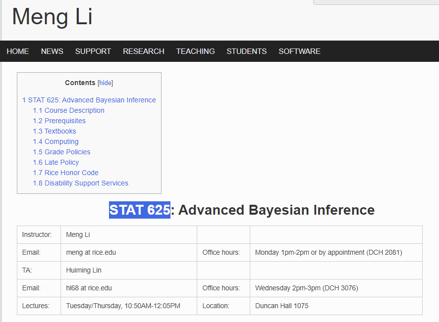
STAT625 Bayesian Analysis课程简介

1. Bayesian inference: This refers to the process of updating prior beliefs or probabilities based on new data or evidence. In Bayesian inference, probabilities are treated as subjective degrees of belief rather than objective frequencies.
2. Advanced Monte Carlo methods: Monte Carlo methods are a class of computational algorithms that use random sampling to obtain numerical solutions to complex problems. Advanced Monte Carlo methods, such as Markov Chain Monte Carlo (MCMC) and Sequential Monte Carlo (SMC), are commonly used in Bayesian inference to simulate from complex posterior distributions.
3. Asymptotic theories: Asymptotic theories provide a framework for understanding the behavior of statistical procedures as the sample size approaches infinity. In Bayesian inference, asymptotic theories can be used to derive the properties of Bayesian estimators and hypothesis tests.
4. Adaptive methods: Adaptive methods refer to techniques that adjust the model or algorithm based on the data at hand. In Bayesian inference, adaptive methods can be used to select the appropriate prior distribution, adjust the tuning parameters of MCMC algorithms, or perform model selection.
5. Bayesian nonparametrics: Bayesian nonparametric models are a class of models that can accommodate complex data structures without specifying a fixed parametric form. Bayesian nonparametric models are flexible and can handle a wide range of data types, such as count data, categorical data, and functional data.

PREREQUISITES 

Here is a tentative course outline with weight in parentheses:

• Methods (1/2): nonparametric Bayes such as Gaussian process, Dirichlet process, Chinese restaurant process, Mixture models, Introduction to asymptotic theory, and variable selection
• Computation (1/3): advanced MCMC such as sequential Monte Carlo, variational methods, convergence assessment, approximation method, and statistical efficiency.
• Application (1/6): selected areas such as machine learning, structural biology, biomedical research (such as brain connectome, neuroimaging), etc.

STAT625 Bayesian Analysis HELP（EXAM HELP， ONLINE TUTOR）

Bayes’ Theorem is a fundamental concept in Bayesian statistics that allows us to update our prior beliefs or probabilities in light of new evidence or data. In simple terms, it provides a framework for calculating the probability of an event based on its prior probability and the probability of the evidence given the event.

To understand how Bayes’ Theorem works, let’s start with the definition of conditional probability. Conditional probability is the probability of an event A given that another event B has occurred. It is denoted as P(A|B) and is calculated as the probability of A and B occurring together divided by the probability of B occurring:

P(A|B) = P(A and B) / P(B)

Now, let’s consider Bayes’ Theorem for point probabilities. Suppose we have a hypothesis H and some observed data D. We want to know the probability of the hypothesis given the data, denoted as P(H|D). Bayes’ Theorem tells us that:

P(H|D) = P(D|H) * P(H) / P(D)

where P(D|H) is the probability of the data given the hypothesis, P(H) is the prior probability of the hypothesis, and P(D) is the probability of the data (also known as the marginal likelihood).

In other words, Bayes’ Theorem tells us that the probability of the hypothesis given the data is proportional to the product of the prior probability of the hypothesis and the probability of the data given the hypothesis, divided by the probability of the data.

By using Bayes’ Theorem, we can update our beliefs about a hypothesis as new data becomes available. We start with a prior probability distribution for the hypothesis, then use Bayes’ Theorem to update the distribution to a posterior probability distribution after observing the data. This allows us to incorporate new information into our analysis and make more informed decisions.

In the pregnancy example, we used a hypothetical pregnancy test with a false positive rate of $5%$ and a false negative rate of $1%$. However, in practice, most pregnancy tests have much lower rates of false positives and false negatives. Instead, pregnancy test accuracy is typically reported as the overall percent of correct results, taking into account both true and false positives and negatives.

Let’s assume that the pregnancy test we are using has an accuracy rate of $90%$. This means that, out of all the cases where the test indicates a positive result, $90%$ of them are true positives, and out of all the cases where the test indicates a negative result, $90%$ of them are true negatives. We can use this information to revise our calculation of the posterior probability of being pregnant given a positive test result.

Recall that the prior probability of being pregnant was $P(pregnant) = 0.01$, and the false positive rate of the test was $P(pos|not~pregnant) = 0.05$. We can now compute the true positive rate of the test as:

$P(pos|pregnant) = 1 – P(neg|pregnant) = 1 – 0.01 = 0.99$

Similarly, the true negative rate of the test is:

$P(neg|notpregnant) = 1 – P(pos|notpregnant) = 1 – 0.9 = 0.1$

Now, using Bayes’ Theorem, we can compute the posterior probability of being pregnant given a positive test result as:

$P(pregnant|pos) = \frac{P(pos|pregnant) \cdot P(pregnant)}{P(pos)}$

where $P(pos)$ is the probability of a positive test result, which can be computed as:

$P(pos) = P(pos|pregnant) \cdot P(pregnant) + P(pos|notpregnant) \cdot P(notpregnant)$

$P(pos) = 0.99 \cdot 0.01 + 0.05 \cdot 0.99 = 0.0585$

Plugging in the values, we get:

$P(pregnant|pos) = \frac{0.99 \cdot 0.01}{0.0585} \approx 0.169$

So, with an accuracy rate of $90%$, the posterior probability of being pregnant given a positive test result is now only about $17%$. The main change in the calculation is that we no longer assume a fixed false positive rate of $5%$. Instead, we take into account the fact that false positives and false negatives occur equally frequently under the $90%$ accuracy rate, and use this information to compute the true positive and true negative rates of the test.

Textbooks

• An Introduction to Stochastic Modeling, Fourth Edition by Pinsky and Karlin (freely
available through the university library here)
• Essentials of Stochastic Processes, Third Edition by Durrett (freely available through
the university library here)
To reiterate, the textbooks are freely available through the university library. Note that
you must be connected to the university Wi-Fi or VPN to access the ebooks from the library
links. Furthermore, the library links take some time to populate, so do not be alarmed if
the webpage looks bare for a few seconds.

Statistics-lab™可以为您提供rice.edu STAT625 Bayesian Analysis贝叶斯分析课程的代写代考和辅导服务！ 请认准Statistics-lab™. Statistics-lab™为您的留学生涯保驾护航。