如果你也在 怎样代写统计模型Statistical Modelling这个学科遇到相关的难题，请随时右上角联系我们的24/7代写客服。

统计建模是使用数学模型和统计假设来生成样本数据并对现实世界进行预测。统计模型是一组实验的所有可能结果的概率分布的集合。

statistics-lab™ 为您的留学生涯保驾护航 在代写统计模型Statistical Modelling方面已经树立了自己的口碑, 保证靠谱, 高质且原创的统计Statistics代写服务。我们的专家在代写统计模型Statistical Modelling代写方面经验极为丰富，各种代写统计模型Statistical Modelling相关的作业也就用不着说。

我们提供的统计模型Statistical Modelling及其相关学科的代写，服务范围广, 其中包括但不限于:

• Statistical Inference 统计推断
• Statistical Computing 统计计算
• Advanced Probability Theory 高等楖率论
• Advanced Mathematical Statistics 高等数理统计学
• (Generalized) Linear Models 广义线性模型
• Statistical Machine Learning 统计机器学习
• Longitudinal Data Analysis 纵向数据分析
• Foundations of Data Science 数据科学基础

统计代写|统计模型作业代写Statistical Modelling代考|Small Sample Refinement: Saddlepoint Approximations

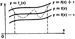
Saddlepoint approximation is a technique for refined approximation of densities and distribution functions when the normal (or $\chi^{2}$ ) approximation is too crude. The method is typically used on distributions for

• Sums of random variables.
• ML estimators.
• Likelihood ratio test statistics,
  and for approximating structure functions. These approximations often have surprisingly small errors, and in some remarkable cases they yield exact results. We confine ourselves to the basics, and consider only density approximation for canonical statistics $t$ (which involves the structure function $g(t)$ ), and for the MLE in any parameterization of the exponential family.
  The saddlepoint approximation for probability densities (continuous distribution case) is due to Daniels (1954). Approximations for distribution functions, being of particular interest for test statistics (for example the so-called Lugannani-Rice formula for the signed log-likelihood ratio), is a more complicated topic, because it will require approximation of integrals of densities instead of just densities, see for example Jensen (1995).

Suppose we have a regular exponential family, with canonical statistic $\boldsymbol{t}$ (no index $n$ here) and canonical parameter $\theta$. If the family is not regular, we restrict $\boldsymbol{\theta}$ to the interior of $\Theta$. Usually $t=t(y)$ has some sort of a sum form, even though the number of terms may be small. We shall derive an approximation for the density $f\left(t ; \theta_{0}\right)$ of $t$, for some specified $\theta=\theta_{0}$. One reason for wanting such an approximation in a given exponential family is the presence of the structure function $g(t)$ in $f\left(t ; \theta_{0}\right)$, which is the factor, often complicated, by which $f\left(t ; \boldsymbol{\theta}{0}\right)$ differs from $f\left(\boldsymbol{y} ; \boldsymbol{\theta}{0}\right)$. Another reason is that we might want the distribution of the ML estimator, and $t=\hat{\boldsymbol{\mu}}_{t}$ is one such MLE.

统计代写|统计模型作业代写Statistical Modelling代考|Extensions and further refinements.

The same technique can at least in principle be used outside exponential families to approximate a density $f(t)$. The idea is to embed $f(t)$ in an exponential family by exponential tilting, see Example $2.12$ with $f(t)$ in the role of its $f_{0}(y)$, For practical use, $f$ must have an explicit and manageable Laplace transform, since the norming constant $C(\boldsymbol{\theta})$ will be the Laplace transform of the density $f$, cf. (3.9).
For iid samples of size $n$ one might guess the error is expressed by a factor of magnitude $1+O(1 / \sqrt{n})$. It is in fact a magnitude better, $1+O(1 / n)$, and this holds uniformly on compact subsets of $\Theta$. The error factor can be further refined by using a more elaborate Edgeworth expansion instead of the simple normal density in the second line of (4.6). An Edgeworth expansion is typically excellent in the centre of the distribution, where it would be used here (for $\boldsymbol{\theta}=\hat{\theta}(t))$. On the other hand, it can be terribly bad in the tails and is generally not advisable for a direct approximation of $f\left(t ; \boldsymbol{\theta}_{0}\right)$. See for example Jensen (1995, Ch. 2) for details and proofs. Such a refinement of the saddlepoint approximation was used by Martin-Löf to prove Boltzmann’s theorem, see Chapter $6 .$

Further refinement is possible, at least in principle, through multiplication by a norming factor such that the density approximation becomes a proper probability density. Note, this factor will typically depend on $\theta_{0}$. Even if the relative approximation error is often remarkably small, it generally depends on the argument $\boldsymbol{t}$. For the distribution of the sample mean it is constant only for three univariate densities of continuous distributions: the normal density, the gamma density, and the inverse Gaussian density (Exercise 4.6). The representation is exact for the normal, see Exercise 4.4, and the inverse Gaussian. For the gamma density the error factor is close to 1, representing the Stirling’s formula approximation of $n$ ! (Section B.2.2). Correction by a norming factor, as mentioned in the previous item, would of course eliminate such a constant relative error, but be pointless in this particular case.
$\Delta$

统计代写|统计模型作业代写Statistical Modelling代考|Saddlepoint approximation for the MLE

The saddlepoint approximation for the density $f\left(\hat{\psi} ; \psi_{0}\right)$ of the $M L$ estimator $\hat{\psi}=\hat{\psi}(t)$ in any smooth parameterization of a regular exponential family is
$$
f\left(\hat{\psi} ; \psi_{0}\right) \approx \frac{\sqrt{\operatorname{det} I(\hat{\psi})}}{(2 \pi)^{k / 2}} \frac{L\left(\psi_{0}\right)}{L(\hat{\psi})}
$$
Here $I(\hat{\psi})$ is the Fisher information for the chosen parameter $\psi$, with inserted $\hat{\psi}$.

Proof We transform from the density for $t=\hat{\mu}{t}$ to the density for $\hat{\psi}(t)$. To achieve this we only have to see the effect of a variable transformation on 4.2 Small Sample Refinement: Saddlepoint Approximations 73 the density. When we replace the variable $\hat{\mu}$, by $\hat{\psi}$, we must also multiply by the Jacobian determinant for the transformation that has Jacobian matrix $\left(\frac{\partial \hat{\mu}{t}}{\partial \bar{\phi}}\right)$. However, this is also precisely what is needed to change the square root of $\operatorname{det} I\left(\mu_{t}\right)=\operatorname{det} V_{t}^{-1}=1 / \operatorname{det} V_{t}$ to take account of the reparameterization, see the Reparameterization lemma, Proposition 3.14. Hence the form of formula (4.9) is invariant under reparameterizations.

Proposition $4.7$ works even much more generally, as shown by BarndorffNielsen and others, and the formula is usually named Barndorff-Nielsen’s formula, or the $p^{*}$ ( ‘ $p$-star’) formula, see Reid (1988) and Barndorff-Nielsen and Cox (1994). Pawitan (2001, Sec. 9.8) refers to it as the ‘magical formula’. The formula holds also after conditioning on distribution-constant (= ancillary) statistics (see Proposition $7.5$ and Remark 7.6), and it holds exactly in transformation models, given the ancillary configuration statistic. It is more complicated to derive outside the exponential families, however, because we cannot then start from (4.7) with the canonical parameter $\boldsymbol{\theta}$ as the parameter of interest.

By analogy with the third item of Remark 4.6 about approximation (4.7), we may here refine (4.9) by replacing the approximate normalization constant $1 / \sqrt{2 \pi}$ by the exact one, that makes the density integrate to 1 .

统计模型代考

统计代写|统计模型作业代写Statistical Modelling代考|Small Sample Refinement: Saddlepoint Approximations

鞍点近似是一种在正态（或χ2) 近似太粗略。该方法通常用于分布

• 随机变量的总和。
• 机器学习估计器。
• 似然比检验统计量，
  用于近似结构函数。这些近似值通常具有令人惊讶的小误差，并且在某些非凡的情况下，它们会产生精确的结果。我们仅限于基础知识，仅考虑规范统计的密度近似吨（其中涉及结构函数G(吨))，对于指数族的任何参数化中的 MLE。
  概率密度的鞍点近似（连续分布情况）归功于 Daniels (1954)。分布函数的近似值，对检验统计特别感兴趣（例如所谓的有符号对数似然比的 Lugannani-Rice 公式），是一个更复杂的主题，因为它需要密度积分的近似值，而不仅仅是密度，例如参见 Jensen (1995)。

假设我们有一个正则指数族，具有典型统计量吨（无索引n这里）和规范参数θ. 如果家庭不规律，我们限制θ到内部θ. 通常吨=吨(是)具有某种求和形式，即使项的数量可能很少。我们将推导出密度的近似值F(吨;θ0)的吨, 对于一些指定的θ=θ0. 在给定的指数族中需要这种近似的一个原因是结构函数的存在G(吨)在F(吨;θ0)，这是一个因素，通常很复杂，通过它F(吨;θ0)不同于F(是;θ0). 另一个原因是我们可能想要 ML 估计器的分布，并且吨=μ^吨就是这样一种 MLE。

统计代写|统计模型作业代写Statistical Modelling代考|Extensions and further refinements.

至少原则上可以在指数族之外使用相同的技术来近似密度F(吨). 这个想法是嵌入F(吨)通过指数倾斜在指数族中，请参见示例2.12和F(吨)在其作用F0(是), 为了实际使用，F必须有一个显式且可管理的拉普拉斯变换，因为规范常数C(θ)将是密度的拉普拉斯变换F，参见。(3.9)。
对于大小的 iid 样本n有人可能会猜测误差是由一个数量级表示的1+这(1/n). 它实际上是一个数量级更好，1+这(1/n), 这在θ. 误差因子可以通过使用更精细的 Edgeworth 展开而不是 (4.6) 第二行中的简单正态密度来进一步细化。Edgeworth 展开通常在分布的中心非常出色，这里将使用它（例如θ=θ^(吨)). 另一方面，尾部可能非常糟糕，通常不建议直接近似F(吨;θ0). 有关详细信息和证明，请参见 Jensen (1995, Ch. 2)。Martin-Löf 使用鞍点近似的这种改进来证明玻尔兹曼定理，参见第6.

至少在原则上，进一步的细化是可能的，通过乘以一个规范因子，使得密度近似成为一个适当的概率密度。请注意，此因素通常取决于θ0. 即使相对近似误差通常非常小，它通常也取决于参数吨. 对于样本均值的分布，它仅对连续分布的三个单变量密度是恒定的：正态密度、伽马密度和逆高斯密度（练习 4.6）。表示法是精确的，见习题 4.4，和逆高斯。对于伽马密度，误差因子接近 1，表示斯特林公式近似n！（第 B.2.2 节）。如上一项所述，通过规范因子进行校正当然会消除这种恒定的相对误差，但在这种特殊情况下毫无意义。
Δ

统计代写|统计模型作业代写Statistical Modelling代考|Saddlepoint approximation for the MLE

密度的鞍点近似F(ψ^;ψ0)的米大号估计器ψ^=ψ^(吨)在正则指数族的任何平滑参数化中
F(ψ^;ψ0)≈这⁡一世(ψ^)(2圆周率)ķ/2大号(ψ0)大号(ψ^)
这里一世(ψ^)是所选参数的 Fisher 信息ψ, 插入ψ^.

证明 我们从密度变换为吨=μ^吨密度为ψ^(吨). 为了实现这一点，我们只需要查看变量变换对 4.2 小样本改进：鞍点近似 73 密度的影响。当我们替换变量时μ^， 经过ψ^，我们还必须乘以雅可比行列式来进行具有雅可比矩阵的变换(∂μ^吨∂φ¯). 然而，这也正是改变平方根所需要的这⁡一世(μ吨)=这⁡在吨−1=1/这⁡在吨要考虑重新参数化，请参见重新参数化引理，命题 3.14。因此，公式（4.9）的形式在重新参数化下是不变的。

主张4.7正如 BarndorffNielsen 和其他人所展示的那样，它的工作原理更加普遍，并且该公式通常被命名为 Barndorff-Nielsen 公式，或者p∗ ( ‘ p-star’) 公式，参见 Reid (1988) 和 Barndorff-Nielsen 和 Cox (1994)。Pawitan (2001, Sec. 9.8) 将其称为“神奇公式”。该公式在以分布常数（=辅助）统计为条件后也成立（见命题7.5和备注 7.6），并且在给定辅助配置统计的情况下，它完全适用于转换模型。然而，在指数族之外推导更复杂，因为我们不能从 (4.7) 开始使用规范参数θ作为感兴趣的参数。

类推 4.6 中关于近似 (4.7) 的第三项，我们可以在这里通过替换近似归一化常数来细化 (4.9)1/2圆周率由确切的一个，这使得密度积分为 1 。

统计代写请认准statistics-lab™. statistics-lab™为您的留学生涯保驾护航。

金融工程代写

金融工程是使用数学技术来解决金融问题。金融工程使用计算机科学、统计学、经济学和应用数学领域的工具和知识来解决当前的金融问题，以及设计新的和创新的金融产品。

非参数统计代写

非参数统计指的是一种统计方法，其中不假设数据来自于由少数参数决定的规定模型；这种模型的例子包括正态分布模型和线性回归模型。

广义线性模型代考

广义线性模型（GLM）归属统计学领域，是一种应用灵活的线性回归模型。该模型允许因变量的偏差分布有除了正态分布之外的其它分布。

术语 广义线性模型（GLM）通常是指给定连续和/或分类预测因素的连续响应变量的常规线性回归模型。它包括多元线性回归，以及方差分析和方差分析（仅含固定效应）。

有限元方法代写

有限元方法（FEM）是一种流行的方法，用于数值解决工程和数学建模中出现的微分方程。典型的问题领域包括结构分析、传热、流体流动、质量运输和电磁势等传统领域。

有限元是一种通用的数值方法，用于解决两个或三个空间变量的偏微分方程（即一些边界值问题）。为了解决一个问题，有限元将一个大系统细分为更小、更简单的部分，称为有限元。这是通过在空间维度上的特定空间离散化来实现的，它是通过构建对象的网格来实现的：用于求解的数值域，它有有限数量的点。边界值问题的有限元方法表述最终导致一个代数方程组。该方法在域上对未知函数进行逼近。[1] 然后将模拟这些有限元的简单方程组合成一个更大的方程系统，以模拟整个问题。然后，有限元通过变化微积分使相关的误差函数最小化来逼近一个解决方案。

tatistics-lab作为专业的留学生服务机构，多年来已为美国、英国、加拿大、澳洲等留学热门地的学生提供专业的学术服务，包括但不限于Essay代写，Assignment代写，Dissertation代写，Report代写，小组作业代写，Proposal代写，Paper代写，Presentation代写，计算机作业代写，论文修改和润色，网课代做，exam代考等等。写作范围涵盖高中，本科，研究生等海外留学全阶段，辐射金融，经济学，会计学，审计学，管理学等全球99%专业科目。写作团队既有专业英语母语作者，也有海外名校硕博留学生，每位写作老师都拥有过硬的语言能力，专业的学科背景和学术写作经验。我们承诺100%原创，100%专业，100%准时，100%满意。

随机分析代写

随机微积分是数学的一个分支，对随机过程进行操作。它允许为随机过程的积分定义一个关于随机过程的一致的积分理论。这个领域是由日本数学家伊藤清在第二次世界大战期间创建并开始的。

时间序列分析代写

随机过程，是依赖于参数的一组随机变量的全体，参数通常是时间。 随机变量是随机现象的数量表现，其时间序列是一组按照时间发生先后顺序进行排列的数据点序列。通常一组时间序列的时间间隔为一恒定值（如1秒，5分钟，12小时，7天，1年），因此时间序列可以作为离散时间数据进行分析处理。研究时间序列数据的意义在于现实中，往往需要研究某个事物其随时间发展变化的规律。这就需要通过研究该事物过去发展的历史记录，以得到其自身发展的规律。

回归分析代写

多元回归分析渐进（Multiple Regression Analysis Asymptotics）属于计量经济学领域，主要是一种数学上的统计分析方法，可以分析复杂情况下各影响因素的数学关系，在自然科学、社会和经济学等多个领域内应用广泛。

MATLAB代写

MATLAB 是一种用于技术计算的高性能语言。它将计算、可视化和编程集成在一个易于使用的环境中，其中问题和解决方案以熟悉的数学符号表示。典型用途包括：数学和计算算法开发建模、仿真和原型制作数据分析、探索和可视化科学和工程图形应用程序开发，包括图形用户界面构建MATLAB 是一个交互式系统，其基本数据元素是一个不需要维度的数组。这使您可以解决许多技术计算问题，尤其是那些具有矩阵和向量公式的问题，而只需用 C 或 Fortran 等标量非交互式语言编写程序所需的时间的一小部分。MATLAB 名称代表矩阵实验室。MATLAB 最初的编写目的是提供对由 LINPACK 和 EISPACK 项目开发的矩阵软件的轻松访问，这两个项目共同代表了矩阵计算软件的最新技术。MATLAB 经过多年的发展，得到了许多用户的投入。在大学环境中，它是数学、工程和科学入门和高级课程的标准教学工具。在工业领域，MATLAB 是高效研究、开发和分析的首选工具。MATLAB 具有一系列称为工具箱的特定于应用程序的解决方案。对于大多数 MATLAB 用户来说非常重要，工具箱允许您学习和应用专业技术。工具箱是 MATLAB 函数（M 文件）的综合集合，可扩展 MATLAB 环境以解决特定类别的问题。可用工具箱的领域包括信号处理、控制系统、神经网络、模糊逻辑、小波、仿真等。

R语言代写	问卷设计与分析代写
PYTHON代写	回归分析与线性模型代写
MATLAB代写	方差分析与试验设计代写
STATA代写	机器学习/统计学习代写
SPSS代写	计量经济学代写
EVIEWS代写	时间序列分析代写
EXCEL代写	深度学习代写
SQL代写	各种数据建模与可视化代写

如果你也在 怎样代写统计模型Statistical Modelling这个学科遇到相关的难题，请随时右上角联系我们的24/7代写客服。

统计建模是使用数学模型和统计假设来生成样本数据并对现实世界进行预测。统计模型是一组实验的所有可能结果的概率分布的集合。

statistics-lab™ 为您的留学生涯保驾护航 在代写统计模型Statistical Modelling方面已经树立了自己的口碑, 保证靠谱, 高质且原创的统计Statistics代写服务。我们的专家在代写统计模型Statistical Modelling代写方面经验极为丰富，各种代写统计模型Statistical Modelling相关的作业也就用不着说。

我们提供的统计模型Statistical Modelling及其相关学科的代写，服务范围广, 其中包括但不限于:

• Statistical Inference 统计推断
• Statistical Computing 统计计算
• Advanced Probability Theory 高等楖率论
• Advanced Mathematical Statistics 高等数理统计学
• (Generalized) Linear Models 广义线性模型
• Statistical Machine Learning 统计机器学习
• Longitudinal Data Analysis 纵向数据分析
• Foundations of Data Science 数据科学基础

统计代写|统计模型作业代写Statistical Modelling代考|Large Sample Asymptotics

For simplicity of notation we suppose the exponential family is regular, so $\boldsymbol{\Theta}$ is open, but the results hold for any full family if $\boldsymbol{\Theta}$ is only restricted to its interior. Proposition $3.10$ showed that the log likelihood function is strictly concave and therefore has a unique maximum, corresponding to a unique root of the likelihood equations, provided there is a (finite) maximal value. We have seen examples in Chapter 3 of likelihoods without a finite maximum, for example in the binomial and Poisson families. We shall here first show that if we have a sample of size $n$ from a regular exponential family, the risk for such an event tends to zero with increasing $n$, and the MLE $\hat{\boldsymbol{\theta}}$ approaches the true $\boldsymbol{\theta}$, i.e. $\hat{\boldsymbol{\theta}}$ is a consistent estimator. The next step, to an asymptotic Gaussian distribution of $\hat{\boldsymbol{\theta}}$, is not big.

We shall use the following notation. Let $t(y)$ be the canonical statistic for a single observation, and $t_{n}=\sum_{i} t\left(y_{i}\right)$ the corresponding canonical statistic for the whole sample. Let $\mu_{t}(\theta)=E_{\theta}{t(y)}=E_{\theta}\left{t_{n} / n\right}$, i.e. the mean value per observational unit. The one-to-one canonical and mean-

value parameterizations by $\boldsymbol{\theta}$ and $\boldsymbol{\mu}$ are related by $\hat{\theta}(\boldsymbol{t})=\boldsymbol{\mu}^{-1}(\boldsymbol{t})$, and for a regular family both $\Theta$ and $\boldsymbol{\mu}(\boldsymbol{\Theta})$ are open sets in $\mathbb{R}^{k}$, where $k=\operatorname{dim} \theta$.

The existence and consistency of the MLE is essentially only a simple application of the law of large numbers under the mean value parameterization (when the MLE is $\hat{\mu}{t}=\boldsymbol{t}{n} / n$ ), followed by a reparameterization. In an analogous way, asymptotic normality of the MLE follows from the central limit theorem applied on $\hat{\mu}_{t}$. However, we will also indicate stronger versions of these results, utilizing more of the exponential family structure.

统计代写|统计模型作业代写Statistical Modelling代考|Existence and consistency of the MLE of θ

For a sample of size n from a regular exponential family, and for any $\boldsymbol{\theta} \in \boldsymbol{\Theta}$,
$$
\operatorname{Pr}\left{\hat{\boldsymbol{\theta}}\left(\boldsymbol{t}{n} / n\right) \text { exists; } \boldsymbol{\theta}\right} \rightarrow 1 \text { as } n \rightarrow \infty, $$ and furthermore, $$ \hat{\boldsymbol{\theta}}\left(\boldsymbol{t}{n} / n\right) \rightarrow \boldsymbol{\theta} \text { in probability as } n \rightarrow \infty
$$
These convergences are uniform on compact subsets of $\Theta$.
Proof By the (weak) law of large numbers (Khinchine version), $t_{n} / n \rightarrow$ $\boldsymbol{\mu}{t}\left(=\boldsymbol{\mu}{t}(\boldsymbol{\theta})\right)$ in probability as $n \rightarrow \infty$. More precisely expressed, for any fixed $\delta>0$,
$$
\operatorname{Pr}\left{\left|\boldsymbol{t}{n} / n-\boldsymbol{\mu}{t}\right|<\delta\right} \rightarrow 1 $$ Note that as soon as $\delta>0$ is small enough, the $\delta$-neighbourhood (4.1) of $\boldsymbol{\mu}{t}$ is wholly contained in the open set $\boldsymbol{\mu}(\boldsymbol{\Theta})$, and that $\boldsymbol{t}{n} / n$ is identical with the MLE $\hat{\boldsymbol{\mu}}{t}$. This is the existence and consistency result for the MLE of the mean value parameter, $\hat{\boldsymbol{\mu}}{t}$. Next we transform this to a result for $\hat{\boldsymbol{\theta}}$ in $\boldsymbol{\Theta}$.
Consider an open $\delta^{\prime}$-neighbourhood of $\theta$. For $\delta^{\prime}>0$ small enough, it is wholly within the open set $\boldsymbol{\Theta}$. There the image function $\boldsymbol{\mu}{t}(\boldsymbol{\theta})$ is welldefined, and the image of the $\delta^{\prime}$-neighbourhood of $\theta$ is an open neighbourhood of $\boldsymbol{\mu}(\boldsymbol{\theta})$ in $\boldsymbol{\mu}(\boldsymbol{\Theta})$ (since $\hat{\boldsymbol{\theta}}=\boldsymbol{\mu}{t}^{-1}$ is a continuous function). Inside that open neighbourhood we can always find (for some $\delta>0$ ) an open $\delta$ neighbourhood of type (4.1), whose probability goes to 1 . Thus, the probability for $\hat{\theta}\left(t_{n} / n\right)$ to be in the $\delta^{\prime}$-neighbourhood of $\theta$ also goes to 1 . This shows the asymptotic existence and consistency of $\hat{\boldsymbol{\theta}}$ for any fixed $\boldsymbol{\theta}$ in $\boldsymbol{\Theta}$.
Finally, this can be strengthened (Martin-Löf, 1970) to uniform convergence on compact subsets of the parameter space $\Theta$. Specifically, Chebyshev’s inequality can be used to give a more explicit upper bound of order $1 / n$ to the complementary probability, $\operatorname{Pr}\left{\left|t_{n} / n-\mu_{t}(\theta)\right| \geq \delta\right}$, proportional to $\operatorname{var}_{t}(\theta)$, that is bounded on compact subsets of $\boldsymbol{\Theta}$, since it is a continuous function of $\theta$. Details are omitted.

统计代写|统计模型作业代写Statistical Modelling代考|Uniform convergence on compacts

General results tells that under a set of suitable regularity conditions, the MLE is correspondingly asymptotically normally distributed as $n \rightarrow \infty$, but with the asymptotic variance expressed as being the inverse of the Fisher information. First note that when we are in a regular exponential family, we require no additional regularity conditions. Secondly, the variance $\operatorname{var}\left(\boldsymbol{t}{n} / n\right)=\operatorname{var}(t) / n$ for $\hat{\boldsymbol{\mu}}{\boldsymbol{t}}$ is precisely the inverse of the Fisher information matrix for $\mu_{t}$ (Proposition $\left.3.15\right)$, and unless $\psi\left(\mu_{t}\right)$ is of lower dimension than $\mu_{t}$ itself, the variance formula in Proposition $4.3$ can alternatively be obtained from $\operatorname{var}(t)$ by use of the Reparameterization lemma (Proposition 3.14). When $\psi$ and $\boldsymbol{\mu}{t}$ are not one-to-one, but $\operatorname{dim} \psi\left(\boldsymbol{\mu}{t}\right)<$ $\operatorname{dim} \mu_{t}$, e.g. $\psi$ a subvector of $\mu_{t}$, the theory of profile likelihoods (Section 3.3.4) can be useful, yielding correct formulas expressed in Fisher information terms. In a concrete situation we are of course free to calculate the estimator variance directly from the explicit form of $\hat{\psi}$. In any case, a conditional inference approach, eliminating nuisance parameters (Section $3.5)$, should also be considered. Asymptotically, however, we should not expect the conditional and unconditional results to differ, unless the nuisance parameters are incidental and increase in number with $n$, as in Exercise 3.16.

Note the special case of the canonical parameterization, with $\boldsymbol{\theta}$ as canonical parameter for the distribution of the single observation $(n=1)$. For this parameter, the asymptotic variance of the MLE is $\operatorname{var}(t)^{-1} / n$, where $t$ is the single observation statistic. This is the special case of Proposition $4.3$ for which
$$
\left(\frac{\partial \psi}{\partial \mu_{t}}\right)=\left(\frac{\partial \theta}{\partial \mu_{t}}\right)=\left(\frac{\partial \mu_{t}}{\partial \theta}\right)^{-1}=\operatorname{var}{\theta}(t)^{-1} $$ Like in the general large sample statistical theory, we may use the result of Proposition $4.3$ to construct asymptotically correct confidence regions. For example, expressed for the canonical parameter $\boldsymbol{\theta}$, it follows from Proposition $4.3$ that the quadratic form in $\hat{\theta}$, $$ Q(\boldsymbol{\theta})=n(\hat{\boldsymbol{\theta}}-\boldsymbol{\theta})^{T} \operatorname{var}{\theta}(\boldsymbol{t})(\hat{\boldsymbol{\theta}}-\boldsymbol{\theta})
$$

统计模型代考

统计代写|统计模型作业代写Statistical Modelling代考|Large Sample Asymptotics

为了符号的简单，我们假设指数族是规则的，所以θ是开放的，但结果适用于任何完整的家庭，如果θ仅限于其内部。主张3.10表明对数似然函数是严格凹的，因此具有唯一的最大值，对应于似然方程的唯一根，前提是存在（有限）最大值。我们已经在第 3 章中看到了没有有限最大值的可能性的例子，例如在二项式和泊松族中。我们将在这里首先证明，如果我们有一个大小为n从正则指数族中，此类事件的风险随着增加而趋于零n, 和 MLEθ^接近真实θ， IEθ^是一致的估计量。下一步，渐近高斯分布θ^，不大。

我们将使用以下符号。让吨(是)是单个观察的典型统计量，并且吨n=∑一世吨(是一世)整个样本的相应规范统计量。让\mu_{t}(\theta)=E_{\theta}{t(y)}=E_{\theta}\left{t_{n} / n\right}\mu_{t}(\theta)=E_{\theta}{t(y)}=E_{\theta}\left{t_{n} / n\right}，即每个观测单位的平均值。一对一的规范和平均

值参数化θ和μ与θ^(吨)=μ−1(吨)，对于普通家庭来说θ和μ(θ)是开集在Rķ， 在哪里ķ=暗淡⁡θ.

MLE的存在性和一致性本质上只是在均值参数化下大数定律的简单应用（当MLE为$\hat{\mu} {t}=\boldsymbol{t} {n} / n),F这ll这在和db是一种r和p一种r一种米和吨和r一世和一种吨一世这n.一世n一种n一种n一种l这G这在s在一种是,一种s是米p吨这吨一世Cn这r米一种l一世吨是这F吨H和米大号和F这ll这在sFr这米吨H和C和n吨r一种ll一世米一世吨吨H和这r和米一种ppl一世和d这n\hat{\mu}_{t}$。但是，我们还将使用更多的指数族结构来指示这些结果的更强版本。

统计代写|统计模型作业代写Statistical Modelling代考|Existence and consistency of the MLE of θ

对于来自正则指数族的大小为 n 的样本，并且对于任何θ∈θ,
\operatorname{Pr}\left{\hat{\boldsymbol{\theta}}\left(\boldsymbol{t}{n} / n\right) \text { 存在；} \boldsymbol{\theta}\right} \rightarrow 1 \text { as } n \rightarrow \infty,\operatorname{Pr}\left{\hat{\boldsymbol{\theta}}\left(\boldsymbol{t}{n} / n\right) \text { 存在；} \boldsymbol{\theta}\right} \rightarrow 1 \text { as } n \rightarrow \infty,此外，θ^(吨n/n)→θ 概率为 n→∞
这些收敛在紧凑子集上是一致的θ.
证明由（弱）大数定律（Khinchin 版本），吨n/n→ μ吨(=μ吨(θ))概率为n→∞. 更准确地说，对于任何固定的d>0,
\operatorname{Pr}\left{\left|\boldsymbol{t}{n} / n-\boldsymbol{\mu}{t}\right|<\delta\right} \rightarrow 1\operatorname{Pr}\left{\left|\boldsymbol{t}{n} / n-\boldsymbol{\mu}{t}\right|<\delta\right} \rightarrow 1请注意，只要d>0足够小，则d- 邻里（4.1）μ吨完全包含在开集中μ(θ)， 然后吨n/n与 MLE 相同μ^吨. 这是均值参数的 MLE 的存在性和一致性结果，μ^吨. 接下来我们将其转换为结果θ^在θ.
考虑一个开放的d′- 邻里θ. 为了d′>0足够小，它完全在开集中θ. 有图像功能μ吨(θ)定义明确，并且图像d′- 邻里θ是一个开放的邻域μ(θ)在μ(θ)（自从θ^=μ吨−1是一个连续函数）。在那个开放的社区里，我们总能找到（对于某些人来说d>0) 一个开放的d类型 (4.1) 的邻域，其概率为 1 。因此，概率为θ^(吨n/n)在d′- 邻里θ也去 1 。这说明了渐近存在性和一致性θ^对于任何固定θ在θ.
最后，这可以得到加强（Martin-Löf，1970）以在参数空间的紧凑子集上均匀收敛θ. 具体来说，切比雪夫不等式可用于给出更明确的阶数上限1/n到互补概率，\operatorname{Pr}\left{\left|t_{n} / n-\mu_{t}(\theta)\right| \geq \delta\right}\operatorname{Pr}\left{\left|t_{n} / n-\mu_{t}(\theta)\right| \geq \delta\right}, 与曾是吨⁡(θ), 是有界的紧子集θ, 因为它是一个连续函数θ. 细节省略。

统计代写|统计模型作业代写Statistical Modelling代考|Uniform convergence on compacts

一般结果表明，在一组合适的正则性条件下，MLE 相应地渐近正态分布为n→∞，但渐近方差表示为 Fisher 信息的倒数。首先请注意，当我们在正则指数族中时，我们不需要额外的正则条件。其次，方差曾是⁡(吨n/n)=曾是⁡(吨)/n为了μ^吨正好是 Fisher 信息矩阵的逆μ吨（主张3.15), 除非ψ(μ吨)比μ吨本身，命题中的方差公式4.3也可以从曾是⁡(吨)通过使用重新参数化引理（命题 3.14）。什么时候ψ和μ吨不是一对一的，而是暗淡⁡ψ(μ吨)< 暗淡⁡μ吨，例如ψ的子向量μ吨，轮廓似然理论（第 3.3.4 节）可能很有用，可以产生用 Fisher 信息项表示的正确公式。在具体情况下，我们当然可以直接从ψ^. 在任何情况下，条件推理方法，消除讨厌的参数（第3.5), 也应该考虑。然而，渐近地，我们不应该期望有条件和无条件的结果会有所不同，除非令人讨厌的参数是偶然的并且随着数量的增加而增加n，如练习 3.16 中所示。

请注意规范参数化的特殊情况，其中θ作为单一观测值分布的规范参数(n=1). 对于该参数，MLE 的渐近方差为曾是⁡(吨)−1/n， 在哪里吨是单一观察统计量。这是命题的特例4.3为此
(∂ψ∂μ吨)=(∂θ∂μ吨)=(∂μ吨∂θ)−1=曾是⁡θ(吨)−1就像在一般的大样本统计理论中，我们可以使用 Proposition 的结果4.3构造渐近正确的置信区域。例如，表示为规范参数θ, 它来自命题4.3二次形式在θ^,问(θ)=n(θ^−θ)吨曾是⁡θ(吨)(θ^−θ)

统计代写请认准statistics-lab™. statistics-lab™为您的留学生涯保驾护航。

金融工程代写

金融工程是使用数学技术来解决金融问题。金融工程使用计算机科学、统计学、经济学和应用数学领域的工具和知识来解决当前的金融问题，以及设计新的和创新的金融产品。

非参数统计代写

非参数统计指的是一种统计方法，其中不假设数据来自于由少数参数决定的规定模型；这种模型的例子包括正态分布模型和线性回归模型。

广义线性模型代考

广义线性模型（GLM）归属统计学领域，是一种应用灵活的线性回归模型。该模型允许因变量的偏差分布有除了正态分布之外的其它分布。

术语 广义线性模型（GLM）通常是指给定连续和/或分类预测因素的连续响应变量的常规线性回归模型。它包括多元线性回归，以及方差分析和方差分析（仅含固定效应）。

有限元方法代写

有限元方法（FEM）是一种流行的方法，用于数值解决工程和数学建模中出现的微分方程。典型的问题领域包括结构分析、传热、流体流动、质量运输和电磁势等传统领域。

有限元是一种通用的数值方法，用于解决两个或三个空间变量的偏微分方程（即一些边界值问题）。为了解决一个问题，有限元将一个大系统细分为更小、更简单的部分，称为有限元。这是通过在空间维度上的特定空间离散化来实现的，它是通过构建对象的网格来实现的：用于求解的数值域，它有有限数量的点。边界值问题的有限元方法表述最终导致一个代数方程组。该方法在域上对未知函数进行逼近。[1] 然后将模拟这些有限元的简单方程组合成一个更大的方程系统，以模拟整个问题。然后，有限元通过变化微积分使相关的误差函数最小化来逼近一个解决方案。

tatistics-lab作为专业的留学生服务机构，多年来已为美国、英国、加拿大、澳洲等留学热门地的学生提供专业的学术服务，包括但不限于Essay代写，Assignment代写，Dissertation代写，Report代写，小组作业代写，Proposal代写，Paper代写，Presentation代写，计算机作业代写，论文修改和润色，网课代做，exam代考等等。写作范围涵盖高中，本科，研究生等海外留学全阶段，辐射金融，经济学，会计学，审计学，管理学等全球99%专业科目。写作团队既有专业英语母语作者，也有海外名校硕博留学生，每位写作老师都拥有过硬的语言能力，专业的学科背景和学术写作经验。我们承诺100%原创，100%专业，100%准时，100%满意。

随机分析代写

随机微积分是数学的一个分支，对随机过程进行操作。它允许为随机过程的积分定义一个关于随机过程的一致的积分理论。这个领域是由日本数学家伊藤清在第二次世界大战期间创建并开始的。

时间序列分析代写

随机过程，是依赖于参数的一组随机变量的全体，参数通常是时间。 随机变量是随机现象的数量表现，其时间序列是一组按照时间发生先后顺序进行排列的数据点序列。通常一组时间序列的时间间隔为一恒定值（如1秒，5分钟，12小时，7天，1年），因此时间序列可以作为离散时间数据进行分析处理。研究时间序列数据的意义在于现实中，往往需要研究某个事物其随时间发展变化的规律。这就需要通过研究该事物过去发展的历史记录，以得到其自身发展的规律。

回归分析代写

多元回归分析渐进（Multiple Regression Analysis Asymptotics）属于计量经济学领域，主要是一种数学上的统计分析方法，可以分析复杂情况下各影响因素的数学关系，在自然科学、社会和经济学等多个领域内应用广泛。

MATLAB代写

MATLAB 是一种用于技术计算的高性能语言。它将计算、可视化和编程集成在一个易于使用的环境中，其中问题和解决方案以熟悉的数学符号表示。典型用途包括：数学和计算算法开发建模、仿真和原型制作数据分析、探索和可视化科学和工程图形应用程序开发，包括图形用户界面构建MATLAB 是一个交互式系统，其基本数据元素是一个不需要维度的数组。这使您可以解决许多技术计算问题，尤其是那些具有矩阵和向量公式的问题，而只需用 C 或 Fortran 等标量非交互式语言编写程序所需的时间的一小部分。MATLAB 名称代表矩阵实验室。MATLAB 最初的编写目的是提供对由 LINPACK 和 EISPACK 项目开发的矩阵软件的轻松访问，这两个项目共同代表了矩阵计算软件的最新技术。MATLAB 经过多年的发展，得到了许多用户的投入。在大学环境中，它是数学、工程和科学入门和高级课程的标准教学工具。在工业领域，MATLAB 是高效研究、开发和分析的首选工具。MATLAB 具有一系列称为工具箱的特定于应用程序的解决方案。对于大多数 MATLAB 用户来说非常重要，工具箱允许您学习和应用专业技术。工具箱是 MATLAB 函数（M 文件）的综合集合，可扩展 MATLAB 环境以解决特定类别的问题。可用工具箱的领域包括信号处理、控制系统、神经网络、模糊逻辑、小波、仿真等。

R语言代写	问卷设计与分析代写
PYTHON代写	回归分析与线性模型代写
MATLAB代写	方差分析与试验设计代写
STATA代写	机器学习/统计学习代写
SPSS代写	计量经济学代写
EVIEWS代写	时间序列分析代写
EXCEL代写	深度学习代写
SQL代写	各种数据建模与可视化代写

如果你也在 怎样代写统计模型Statistical Modelling这个学科遇到相关的难题，请随时右上角联系我们的24/7代写客服。

统计建模是使用数学模型和统计假设来生成样本数据并对现实世界进行预测。统计模型是一组实验的所有可能结果的概率分布的集合。

statistics-lab™ 为您的留学生涯保驾护航 在代写统计模型Statistical Modelling方面已经树立了自己的口碑, 保证靠谱, 高质且原创的统计Statistics代写服务。我们的专家在代写统计模型Statistical Modelling代写方面经验极为丰富，各种代写统计模型Statistical Modelling相关的作业也就用不着说。

我们提供的统计模型Statistical Modelling及其相关学科的代写，服务范围广, 其中包括但不限于:

• Statistical Inference 统计推断
• Statistical Computing 统计计算
• Advanced Probability Theory 高等楖率论
• Advanced Mathematical Statistics 高等数理统计学
• (Generalized) Linear Models 广义线性模型
• Statistical Machine Learning 统计机器学习
• Longitudinal Data Analysis 纵向数据分析
• Foundations of Data Science 数据科学基础

统计代写|统计模型作业代写Statistical Modelling代考|Newton–Raphson, Fisher Scoring and Other Algorithms

For a full family in mean value parameterization the MLE is evidently explicit, $\hat{\boldsymbol{\mu}}{t}=\boldsymbol{t}$. For other parameterizations, by some $\psi$ say, we must invert the equation system $\mu{t}(\hat{\psi})=t$, and this need not have an explicit solution.
A classic and presumably well-known algorithm for iterative solution of equation systems is the Newton-Raphson method. Its basis here is the following linearization of the score $U$, which is adequate for $\psi$ close enough to the unknown $\hat{\psi}$ (note that $-J$ is the Hessian matrix of partial derivatives of $U$ ):
$$
0=U_{\psi}(\hat{\psi}) \approx U_{\dot{\psi}}(\psi)-J_{\psi}(\psi)(\hat{\psi}-\psi) .
$$
Iteratively solving for $\hat{\psi}$ in this linearized system yields successive updates of $\psi_{k}$ to $\psi_{k+1}, k=0,1,2, \ldots .$
$$
\psi_{k+1}=\psi_{k}+J_{\psi}\left(\psi_{k}\right)^{-1} U_{\psi}\left(\psi_{k}\right)
$$
This is a locally fast algorithm (quadratic convergence), provided that it converges. The method can be quite sensitive to the choice of starting point $\psi_{0^{}}$ Generally, if $J_{\psi^{}}\left(\psi_{0}\right)$ is not positive definite or close to singular, it is not likely to converge, or it might converge to a minimum of $\log L$, so there is no guarantee that the resulting root represents even a local likelihood maximum. For a full exponential family, however, the odds are better. In particular, there is not more than one root, and if the parameter is the canonical, $\boldsymbol{\theta}$, we know that $J_{\theta}=I_{\theta}=\operatorname{var}(\boldsymbol{t})$, a necessarily positive definite matrix. Quasi-Newton methods are modifications of $(3.27)$, where the $J$ matrix is approximated, e.g. by the secant method, typically because an explicit formula for $J$ is not available.

统计代写|统计模型作业代写Statistical Modelling代考|Conditional Inference for Canonical Parameter

Suppose $\psi$ is a parameter of interest, either being itself a subvector $\theta_{v}$ of $\boldsymbol{\theta}$, perhaps after a linear transformation of the canonical statistic $\boldsymbol{t}$, or being

some other one-to-one function of $\theta_{v}$. Corresponding to the partitioning $t=(u, v)$, we may write $\theta$ as $(\lambda, \psi)$. Here $\lambda$, represented by $\theta_{u}$ or $\mu_{u}$, is regarded as a nuisance parameter, supplementing $\psi$. As shown in Section $3.3 .3$ above, $\lambda=\boldsymbol{\mu}{u}=E{\theta}(\boldsymbol{u})$ is the preferable nuisance parameter, at least in principle, since $\psi$ and $\boldsymbol{\mu}{u}$ are variation independent and information orthogonal (Proposition $3.20$ ). Proposition $3.21$ Conditionality principle for full families Statistical inference about the canonical parameter component $\psi$ in presence of the nuisance parameter $\lambda$ or $\boldsymbol{\mu}{\mathrm{u}}=E_{\theta}(\boldsymbol{u})$ should be made conditional on $\boldsymbol{u}$, that is, in the conditional model for $\boldsymbol{y}$ or $\boldsymbol{v}$ given $\boldsymbol{u}$.
Motivation. The likelihood for $\left(\mu_{u}, \psi\right)$ factorizes as
$$
L\left(\boldsymbol{\mu}{u}, \psi ; t\right)=L{1}\left(\boldsymbol{\mu}{u}, \psi ; u\right) L{2}(\psi ; \boldsymbol{v} \mid \boldsymbol{u}),
$$
where the two parameters are variation independent. In some cases, exemplified by Example 3.2, $L_{1}$ depends only on $\boldsymbol{\mu}{u}$, $$ L\left(\mu{u}, \psi ; t\right)=L_{1}\left(\mu_{u} ; u\right) L_{2}(\psi ; v \mid u) .
$$
Then it is clear that there is no information whatsoever about $\psi$ in the first factor $L_{1}$, and the argument for the principle is compelling. The terminology for this situation is that the factorization is called a cut, and $\boldsymbol{u}$ is called $S$-ancillary for $\psi$. But also when $L_{1}$ depends on $\psi$ (illustrated in Example $3.3$ ), there is really no information about $\psi$ in $u$, as seen by the following argument. Note first that $u$ and $\boldsymbol{\mu}{u}$ are of the same dimension (of course), and that $\boldsymbol{u}$ serves as an estimator (the MLE) of $\boldsymbol{\mu}{u}$, whatever be $\psi$ (Proposition 3.11). This means that the information in $\boldsymbol{u}$ about $\left(\mu_{u}, \psi\right)$ is totally consumed in the estimation of $\mu_{u}$. Furthermore, the estimated value of $\mu_{u}$ does not provide any information about $\psi$, and $\mu_{u}$ would not do so even if it were known, due to the variation independence between $\mu_{u}$ and $\psi$. Thus, the first factor $L_{1}$ contributes only information about $\mu_{u}$ in (3.28).

统计代写|统计模型作业代写Statistical Modelling代考|Two Poisson variates

Suppose we want to make inference about the relative change in a Poisson parameter from one occasion to another, with one observation per occasion.
$48 \quad$ Regularity Conditions and Basic Properties
Specifically, let $y_{1}$ and $y_{2}$ be independent Poisson distributed variables with mean values $e^{\lambda}$ and $e^{\psi+\lambda}$, respectively. The model is
$$
f\left(y_{1}, y_{2} ; \lambda, \psi\right)=\frac{h\left(y_{1}, y_{2}\right)}{C(\lambda, \psi)} e^{\lambda\left(y_{1}+y_{2}\right)+\psi y_{2}}
$$
The parameter of prime interest is $e^{\phi}$, or equivalently the canonical $\psi$. The conditionality principle states that the inference about $\psi$ should be made in the conditional model for $v=y_{2}$ given the other canonical statistic $u=$ $y_{1}+y_{2}$. Simple but important calculations left as an exercise (Exercise 3.13) show that this model is the binomial distribution with logit parameter $\psi$, $\operatorname{Bin}\left{y_{1}+y_{2} ; e^{\psi} /\left(1+e^{\psi}\right)\right}$. The marginal distribution for $u=y_{1}+y_{2}$ is $\operatorname{Po}\left(\mu_{u}\right)$, not additionally involving $\psi$. Thus we have a cut, and $S$-ancillarity. Note the crucial role of the mixed parameterization to obtain a cut. If expressed instead in terms of the canonical parameters $\lambda$ and $\psi$ of the joint model, the Poisson parameter in the marginal for $u$ would have been dependent on both $\lambda$ and $\psi$, since $\mu_{u}=E\left(y_{1}+y_{2}\right)=e^{\lambda}\left(1+e^{\phi}\right)$.

Under S-ancillarity, the MLEs will be the same when derived in the conditional or marginal models as in the joint model, and the observed and expected information matrices in the joint model will be block diagonal with blocks representing the conditional and marginal models. This can sometimes be used in the opposite way, by artificially extending a conditionally defined model to a simpler joint model with the same MLEs etc, see Section 5.6. Outside S-ancillarity we cannot count on these properties, but we must instead distinguish joint model and conditional model MLEs. Here is one such example, see Example $3.6$ for another one.

统计模型代考

统计代写|统计模型作业代写Statistical Modelling代考|Newton–Raphson, Fisher Scoring and Other Algorithms

对于平均值参数化的全族，MLE 显然是明确的，μ^吨=吨. 对于其他参数化，由一些ψ说，我们必须反转方程组μ吨(ψ^)=吨，并且这不需要明确的解决方案。
用于迭代求解方程组的经典且可能众所周知的算法是 Newton-Raphson 方法。这里的基础是分数的以下线性化在，这对于ψ足够接近未知ψ^（注意−Ĵ是偏导数的 Hessian 矩阵在 ):
0=在ψ(ψ^)≈在ψ˙(ψ)−Ĵψ(ψ)(ψ^−ψ).
迭代求解ψ^在这个线性化系统中产生的连续更新ψķ到ψķ+1,ķ=0,1,2,….
ψķ+1=ψķ+Ĵψ(ψķ)−1在ψ(ψķ)
这是一种局部快速算法（二次收敛），前提是它收敛。该方法对起点的选择非常敏感ψ0一般来说，如果Ĵψ(ψ0)不是正定的或接近奇异的，它不可能收敛，或者它可能收敛到最小值日志⁡大号，因此不能保证生成的根甚至代表局部似然最大值。然而，对于一个完整的指数家庭，可能性更大。特别是，不超过一个根，如果参数是规范的，θ， 我们知道Ĵθ=一世θ=曾是⁡(吨)，一个必然的正定矩阵。准牛顿方法是对(3.27), 其中Ĵ矩阵是近似的，例如通过割线法，通常是因为一个明确的公式Ĵ不可用。

统计代写|统计模型作业代写Statistical Modelling代考|Conditional Inference for Canonical Parameter

认为ψ是一个感兴趣的参数，或者本身就是一个子向量θ在的θ，也许在典型统计量的线性变换之后吨，或者是

的其他一些一对一功能θ在. 对应分区吨=(在,在)，我们可以写θ作为(λ,ψ). 这里λ，表示为θ在或者μ在, 被认为是一个讨厌的参数，补充ψ. 如部分所示3.3.3多于，λ=μ在=和θ(在)是优选的有害参数，至少在原则上，因为ψ和μ在是变化独立和信息正交（命题3.20）。主张3.21全族的条件性原则关于规范参数分量的统计推断ψ在存在令人讨厌的参数的情况下λ或者μ在=和θ(在)应以在，也就是说，在条件模型中是或者在给定在.
动机。可能性为(μ在,ψ)分解为
大号(μ在,ψ;吨)=大号1(μ在,ψ;在)大号2(ψ;在∣在),
其中两个参数与变化无关。在某些情况下，以示例 3.2 为例，大号1只取决于μ在,大号(μ在,ψ;吨)=大号1(μ在;在)大号2(ψ;在∣在).
那么很明显，没有任何关于ψ在第一个因素大号1，并且该原则的论据是令人信服的。这种情况的术语是分解称为割，并且在叫做小号- 辅助ψ. 但也当大号1取决于ψ（在示例中说明3.3)，确实没有关于ψ在在，如以下论点所示。首先注意在和 $\boldsymbol{\mu} {u}一种r和这F吨H和s一种米和d一世米和ns一世这n(这FC这在rs和),一种nd吨H一种吨\boldsymbol{u}s和r在和s一种s一种n和s吨一世米一种吨这r(吨H和米大号和)这F\boldsymbol {\ mu} {u},在H一种吨和在和rb和\psi(磷r这p这s一世吨一世这n3.11).吨H一世s米和一种ns吨H一种吨吨H和一世nF这r米一种吨一世这n一世n\boldsymbol{u}一种b这在吨\左（\ mu_ {u}，\ psi \右）一世s吨这吨一种ll是C这ns在米和d一世n吨H和和s吨一世米一种吨一世这n这F\ mu_ {u}.F在r吨H和r米这r和,吨H和和s吨一世米一种吨和d在一种l在和这F\ mu_ {u}d这和sn这吨pr这在一世d和一种n是一世nF这r米一种吨一世这n一种b这在吨\psi,一种nd\ mu_ {u}在这在ldn这吨d这s这和在和n一世F一世吨在和r和ķn这在n,d在和吨这吨H和在一种r一世一种吨一世这n一世nd和p和nd和nC和b和吨在和和n\ mu_ {u}一种nd\psi.吨H在s,吨H和F一世rs吨F一种C吨这rL_{1}C这n吨r一世b在吨和s这nl是一世nF这r米一种吨一世这n一种b这在吨\ mu_ {u} $ in (3.28)。

统计代写|统计模型作业代写Statistical Modelling代考|Two Poisson variates

假设我们想推断泊松参数从一种情况到另一种情况的相对变化，每次观察一次。
48正则性条件和基本性质
具体来说，让是1和是2是具有平均值的独立泊松分布变量和λ和和ψ+λ， 分别。模型是
F(是1,是2;λ,ψ)=H(是1,是2)C(λ,ψ)和λ(是1+是2)+ψ是2
最感兴趣的参数是和φ，或等价的规范ψ. 条件性原则表明，关于ψ应在条件模型中进行在=是2给定其他典型统计量在= 是1+是2. 作为练习（练习 3.13）留下的简单但重要的计算表明该模型是带有 logit 参数的二项式分布ψ, \operatorname{Bin}\left{y_{1}+y_{2} ; e^{\psi} /\left(1+e^{\psi}\right)\right}\operatorname{Bin}\left{y_{1}+y_{2} ; e^{\psi} /\left(1+e^{\psi}\right)\right}. 边际分布为在=是1+是2是后⁡(μ在), 不另外涉及ψ. 因此我们有一个切口，并且小号-辅助性。请注意混合参数化对获得切割的关键作用。如果用规范参数表示λ和ψ联合模型的边缘泊松参数在将依赖于两者λ和ψ， 自从μ在=和(是1+是2)=和λ(1+和φ).

在 S 辅助性下，在条件或边际模型中导出的 MLE 将与在联合模型中的相同，并且联合模型中的观察和预期信息矩阵将是块对角线，块代表条件和边际模型。这有时可以以相反的方式使用，通过人为地将条件定义的模型扩展到具有相同 MLE 等的更简单的联合模型，请参见第 5.6 节。在 S 辅助性之外，我们不能指望这些属性，而是必须区分联合模型和条件模型 MLE。这是一个这样的示例，请参阅示例3.6对于另一个。

统计代写请认准statistics-lab™. statistics-lab™为您的留学生涯保驾护航。

金融工程代写

金融工程是使用数学技术来解决金融问题。金融工程使用计算机科学、统计学、经济学和应用数学领域的工具和知识来解决当前的金融问题，以及设计新的和创新的金融产品。

非参数统计代写

非参数统计指的是一种统计方法，其中不假设数据来自于由少数参数决定的规定模型；这种模型的例子包括正态分布模型和线性回归模型。

广义线性模型代考

广义线性模型（GLM）归属统计学领域，是一种应用灵活的线性回归模型。该模型允许因变量的偏差分布有除了正态分布之外的其它分布。

术语 广义线性模型（GLM）通常是指给定连续和/或分类预测因素的连续响应变量的常规线性回归模型。它包括多元线性回归，以及方差分析和方差分析（仅含固定效应）。

有限元方法代写

有限元方法（FEM）是一种流行的方法，用于数值解决工程和数学建模中出现的微分方程。典型的问题领域包括结构分析、传热、流体流动、质量运输和电磁势等传统领域。

有限元是一种通用的数值方法，用于解决两个或三个空间变量的偏微分方程（即一些边界值问题）。为了解决一个问题，有限元将一个大系统细分为更小、更简单的部分，称为有限元。这是通过在空间维度上的特定空间离散化来实现的，它是通过构建对象的网格来实现的：用于求解的数值域，它有有限数量的点。边界值问题的有限元方法表述最终导致一个代数方程组。该方法在域上对未知函数进行逼近。[1] 然后将模拟这些有限元的简单方程组合成一个更大的方程系统，以模拟整个问题。然后，有限元通过变化微积分使相关的误差函数最小化来逼近一个解决方案。

tatistics-lab作为专业的留学生服务机构，多年来已为美国、英国、加拿大、澳洲等留学热门地的学生提供专业的学术服务，包括但不限于Essay代写，Assignment代写，Dissertation代写，Report代写，小组作业代写，Proposal代写，Paper代写，Presentation代写，计算机作业代写，论文修改和润色，网课代做，exam代考等等。写作范围涵盖高中，本科，研究生等海外留学全阶段，辐射金融，经济学，会计学，审计学，管理学等全球99%专业科目。写作团队既有专业英语母语作者，也有海外名校硕博留学生，每位写作老师都拥有过硬的语言能力，专业的学科背景和学术写作经验。我们承诺100%原创，100%专业，100%准时，100%满意。

随机分析代写

随机微积分是数学的一个分支，对随机过程进行操作。它允许为随机过程的积分定义一个关于随机过程的一致的积分理论。这个领域是由日本数学家伊藤清在第二次世界大战期间创建并开始的。

时间序列分析代写

随机过程，是依赖于参数的一组随机变量的全体，参数通常是时间。 随机变量是随机现象的数量表现，其时间序列是一组按照时间发生先后顺序进行排列的数据点序列。通常一组时间序列的时间间隔为一恒定值（如1秒，5分钟，12小时，7天，1年），因此时间序列可以作为离散时间数据进行分析处理。研究时间序列数据的意义在于现实中，往往需要研究某个事物其随时间发展变化的规律。这就需要通过研究该事物过去发展的历史记录，以得到其自身发展的规律。

回归分析代写

多元回归分析渐进（Multiple Regression Analysis Asymptotics）属于计量经济学领域，主要是一种数学上的统计分析方法，可以分析复杂情况下各影响因素的数学关系，在自然科学、社会和经济学等多个领域内应用广泛。

MATLAB代写

MATLAB 是一种用于技术计算的高性能语言。它将计算、可视化和编程集成在一个易于使用的环境中，其中问题和解决方案以熟悉的数学符号表示。典型用途包括：数学和计算算法开发建模、仿真和原型制作数据分析、探索和可视化科学和工程图形应用程序开发，包括图形用户界面构建MATLAB 是一个交互式系统，其基本数据元素是一个不需要维度的数组。这使您可以解决许多技术计算问题，尤其是那些具有矩阵和向量公式的问题，而只需用 C 或 Fortran 等标量非交互式语言编写程序所需的时间的一小部分。MATLAB 名称代表矩阵实验室。MATLAB 最初的编写目的是提供对由 LINPACK 和 EISPACK 项目开发的矩阵软件的轻松访问，这两个项目共同代表了矩阵计算软件的最新技术。MATLAB 经过多年的发展，得到了许多用户的投入。在大学环境中，它是数学、工程和科学入门和高级课程的标准教学工具。在工业领域，MATLAB 是高效研究、开发和分析的首选工具。MATLAB 具有一系列称为工具箱的特定于应用程序的解决方案。对于大多数 MATLAB 用户来说非常重要，工具箱允许您学习和应用专业技术。工具箱是 MATLAB 函数（M 文件）的综合集合，可扩展 MATLAB 环境以解决特定类别的问题。可用工具箱的领域包括信号处理、控制系统、神经网络、模糊逻辑、小波、仿真等。

R语言代写	问卷设计与分析代写
PYTHON代写	回归分析与线性模型代写
MATLAB代写	方差分析与试验设计代写
STATA代写	机器学习/统计学习代写
SPSS代写	计量经济学代写
EVIEWS代写	时间序列分析代写
EXCEL代写	深度学习代写
SQL代写	各种数据建模与可视化代写

如果你也在 怎样代写统计模型Statistical Modelling这个学科遇到相关的难题，请随时右上角联系我们的24/7代写客服。

统计建模是使用数学模型和统计假设来生成样本数据并对现实世界进行预测。统计模型是一组实验的所有可能结果的概率分布的集合。

statistics-lab™ 为您的留学生涯保驾护航 在代写统计模型Statistical Modelling方面已经树立了自己的口碑, 保证靠谱, 高质且原创的统计Statistics代写服务。我们的专家在代写统计模型Statistical Modelling代写方面经验极为丰富，各种代写统计模型Statistical Modelling相关的作业也就用不着说。

我们提供的统计模型Statistical Modelling及其相关学科的代写，服务范围广, 其中包括但不限于:

• Statistical Inference 统计推断
• Statistical Computing 统计计算
• Advanced Probability Theory 高等楖率论
• Advanced Mathematical Statistics 高等数理统计学
• (Generalized) Linear Models 广义线性模型
• Statistical Machine Learning 统计机器学习
• Longitudinal Data Analysis 纵向数据分析
• Foundations of Data Science 数据科学基础

统计代写|统计模型作业代写Statistical Modelling代考|Reparameterization lemma

If $\psi$ and $\theta=\theta(\psi)$ are two equivalent parameterizations of the same model, or if parameterization by $\psi$ represents a lower-dimensional subfamily of a family parameterized by $\boldsymbol{\theta}$, via $\boldsymbol{\theta}=\boldsymbol{\theta}(\boldsymbol{\psi})$, then the score functions are related by
$$
U_{\dot{\psi}}(\psi ; y)=\left(\frac{\partial \boldsymbol{\theta}}{\partial \psi}\right)^{T} U_{\theta}(\boldsymbol{\theta}(\psi) ; \boldsymbol{y}),
$$
and the corresponding information matrices are related by the equations
$$
\begin{aligned}
&I_{\psi}(\psi)=\left(\frac{\partial \theta}{\partial \psi}\right)^{T} I_{\theta}(\theta(\psi))\left(\frac{\partial \theta}{\partial \psi}\right) \
&J_{\psi}(\hat{\psi})=\left(\frac{\partial \theta}{\partial \psi}\right)^{T} J_{\theta}(\theta(\hat{\psi}))\left(\frac{\partial \theta}{\partial \psi}\right)
\end{aligned}
$$
where the information matrices refer to their respective parameterizations and are calculated in points $\psi$ and $\theta(\psi)$, respectively, and where $\left(\frac{\partial \theta}{\partial \psi}\right)$ is the Jacobian transformation matrix for the reparameterization, calculated in the same point as the information matrix.

Note that it is generally crucial to distinguish the Jacobian matrix from its transpose. The definition of the Jacobian is such that the $(i, j)$ element of $\left(\frac{\partial \theta}{\partial \psi}\right)$ is the partial derivative of $\theta_{i}$ with respect to $\psi_{j}$.

When $\psi$ and $\theta$ are two equivalent parameterizations, it is sometimes easier to derive $\left(\frac{\partial \varphi}{\partial \theta}\right)$ than $\left(\frac{\partial \theta}{\partial \psi}\right)$ for use in the reparameterization expressions. Note then that they are the inverses of each other, cf. Section B.2.

Note also that Proposition $3.14$ does not allow $\psi$ to be a function of $\boldsymbol{\theta}$, so for example not a component or subvector of $\boldsymbol{\theta}$. Reducing the score to a subvector of itself, and the information matrix to the corresponding

submatrix, is legitimate only when the excluded parameter subvector is regarded as known (cf. Proposition 4.3).

Note finally that the relationship (3.16) between the two Fisher informations $I$ holds for any $\psi$, whereas the corresponding relation (3.17) for the observed information $J$ only holds in the ML point. The reason for the latter fact will be clear from the following proof.
Proof Repeated use of the chain rule for differentiation yields first
$$
D_{\varphi} \log L=\left(\frac{\partial \theta}{\partial \psi}\right)^{T} D_{\theta} \log L
$$
and next
$$
D_{\psi}^{2} \log L=\left(\frac{\partial \theta}{\partial \psi}\right)^{T} D_{\theta}^{2} \log L\left(\frac{\partial \theta}{\partial \psi}\right)+\left(\frac{\partial^{2} \theta}{\partial \psi^{2}}\right)^{T} D_{\theta} \log L
$$
where the last term represents a matrix obtained when the three-dimensional array $\left(\frac{\partial^{2} \theta}{\partial \psi^{2}}\right)^{T}$ is multiplied by a vector. In the MLE point this last term of (3.19) vanishes, since $D_{\theta} \log L=0$, and (3.17) is obtained. Also, if we take expected values, the same term vanishes because the score function has expected value zero, and the corresponding relation between the expected informations follows.

统计代写|统计模型作业代写Statistical Modelling代考|Mixed parameterization

The mixed parameterization is a valid parameterization.
Proof of Corollary $3.17$ From Proposition $3.16$ it follows that the conditional density can be parameterized by $\theta_{v}$. When $\theta_{v}$ has been specified, Proposition $3.16$ additionally tells that the marginal for $u$ is an exponential family that is for example parameterized by its mean value $\mu_{u}$. Finally, since the joint density for $u$ and $v$ is the product of these marginal and conditional densities, it follows that the mixed parameterization with $\left(\mu_{u}, \theta_{v}\right)$ is also a valid parameterization of the family for $t$.

Proof of Proposition $3.16$ The marginal density for $\boldsymbol{u}$ is obtained by integrating the density (1.8) for $\boldsymbol{t}$ with respect to $\boldsymbol{v}$, for fixed $\boldsymbol{u}$ :
$$
\begin{aligned}
f(\boldsymbol{u} ; \boldsymbol{\theta}) &=\int a(\boldsymbol{\theta}) g(\boldsymbol{u}, \boldsymbol{v}) e^{\boldsymbol{\theta}{u}^{T}} \boldsymbol{u}+\boldsymbol{\theta}{v}^{T} \boldsymbol{v}{\mathrm{d} \boldsymbol{v}} \ &=a(\boldsymbol{\theta}) e^{\boldsymbol{\theta}{u}^{T} \boldsymbol{u}} \int g(\boldsymbol{u}, \boldsymbol{v}) e^{\boldsymbol{\theta}{v}^{T} \boldsymbol{v}} \mathrm{d} \boldsymbol{v} \end{aligned} $$ The integral factor on the second line is generally a function of both data and the parameter $\left(\theta{v}\right)$, which destroys the exponential family property. However, for each given $\theta_{v}$, this factor is only a function of data, and then the family is exponential. Its canonical parameter is $\theta_{u}$, but the parameter space for $\boldsymbol{\theta}{u}$ may depend on $\boldsymbol{\theta}{v}$, being the intersection of $\boldsymbol{\Theta}$ with the hyperplane or affine subspace $\theta_{v}=$ fixed. Since this exponential family

is automatically regular in $\theta_{u}$, the range for its mean value $\mu_{u}$, that is, its mean value parameter space, is identical with the interior of the closed convex hull of the support of the family of distributions for $u$, according to Proposition 3.13. However, since this set is independent of $\theta_{v}$, the parameter space for $\mu_{u}$ is also independent of $\theta_{v}$, as was to be shown.

For the conditional model we do not bother about possible mathematical technicalities connected with conditional densities, but simply write as for conditional probabilities, using the marginal density (3.21) to simplify for $\boldsymbol{u}=\boldsymbol{u}(\boldsymbol{y})$ the expression:
$$
\begin{aligned}
f(\boldsymbol{y} \mid \boldsymbol{u} ; \boldsymbol{\theta}) &=f(\boldsymbol{u}, \boldsymbol{y} ; \boldsymbol{\theta}) / f(\boldsymbol{u} ; \boldsymbol{\theta}) \
&=\frac{e^{\boldsymbol{\theta}{\leftarrow}^{T} v(\boldsymbol{v})} h(\boldsymbol{y})}{\int e^{\theta{r}^{T} v} g(\boldsymbol{u}, \boldsymbol{v}) \mathrm{d} v} .
\end{aligned}
$$
To obtain $f(\boldsymbol{v} \mid \boldsymbol{u} ; \boldsymbol{\theta})$ we only substitute $g(\boldsymbol{u}, \boldsymbol{v})$ for $h(\boldsymbol{y})$ in the numerator of the exponential family density (3.22). Note that $f(\boldsymbol{v} \mid \boldsymbol{u} ; \boldsymbol{\theta})$ is defined only for those $v$-values which are possible for the given $u$, and the denominator is the integral over this set of values. This makes the model depend on $u$, even though the canonical parameter is the same, $\boldsymbol{\theta}_{v}$, and in particular the conditional mean and variance of $v$ will usually depend on $u$.

统计代写|统计模型作业代写Statistical Modelling代考|Marginality and conditionality for Gaussian sample

As an illustration of Proposition 3.16, consider $u=\sum y_{i}^{2}$ for a sample from the normal distribution, with $v=\sum y_{i}$. First, the marginal distribution of $\sum y_{i}^{2}$ is proportional to a noncentral $\chi^{2}$ and does not in general form an exponential family. Next, consider instead its conditional distribution, given $\sum y_{i}=n \bar{y}$. This might appear quite complicated, but given $\bar{y}, \sum y_{i}^{2}$ differs by only an additive, known constant from $\sum y_{i}^{2}-n \bar{y}^{2}=(n-1) s^{2}$. Thus, it is enough to characterize the distribution of $(n-1) s^{2}$, and it is well-known that $s^{2}$ is independent of $\bar{y}$ (see also Section 3.7), and that the distribution of $(n-1) s^{2}$ is proportional (by $\sigma^{2}$ ) to a (central) $\chi^{2}(n-1)$. From the explicit form of a $\chi^{2}$ it is easily seen that the conditional distribution forms an exponential family (Reader, check!).

The canonical parameter space for the conditional family is at least as large as the maximal set of $\boldsymbol{\theta}{v}$-values in $\boldsymbol{\Theta}$, that is, the set of $\boldsymbol{\theta}{v}$ such that $\left(\boldsymbol{\theta}{u}, \boldsymbol{\theta}{v}\right) \in \boldsymbol{\Theta}$ for some $\boldsymbol{\theta}{u}$. Typically the two sets are the same, but there are models in which the conditional canonical parameter space is actually larger and includes parameter values $\boldsymbol{\theta}{v}$ that lack interpretation in the joint model, see for example the Strauss model in Section 13.1.2 and the model in Section 14.3(b).

统计模型代考

统计代写|统计模型作业代写Statistical Modelling代考|Reparameterization lemma

如果ψ和θ=θ(ψ)是同一模型的两个等效参数化，或者如果参数化通过ψ表示由以下参数化的族的低维子族θ， 通过θ=θ(ψ)，那么得分函数与
在ψ˙(ψ;是)=(∂θ∂ψ)吨在θ(θ(ψ);是),
和相应的信息矩阵由方程相关
一世ψ(ψ)=(∂θ∂ψ)吨一世θ(θ(ψ))(∂θ∂ψ) Ĵψ(ψ^)=(∂θ∂ψ)吨Ĵθ(θ(ψ^))(∂θ∂ψ)
其中信息矩阵指的是它们各自的参数化并以点为单位计算ψ和θ(ψ)，分别在哪里(∂θ∂ψ)是用于重新参数化的雅可比变换矩阵，在与信息矩阵相同的点处计算。

请注意，将雅可比矩阵与其转置区分开来通常至关重要。雅可比的定义是这样的(一世,j)的元素(∂θ∂ψ)是的偏导数θ一世关于ψj.

什么时候ψ和θ是两个等价的参数化，有时更容易推导(∂披∂θ)比(∂θ∂ψ)用于重新参数化表达式。请注意，它们是彼此的倒数，参见。B.2 节。

还要注意，命题3.14不允许ψ成为一个函数θ，因此例如不是的分量或子向量θ. 将分数降为自身的一个子向量，将信息矩阵降为对应的

子矩阵，仅当排除的参数子向量被认为是已知的时才是合法的（参见命题 4.3）。

最后注意两个Fisher信息之间的关系（3.16）一世适用于任何ψ, 而观测信息的对应关系 (3.17)Ĵ只在 ML 点成立。后一事实的原因将从以下证明中清楚。
证明重复使用链式法则进行微分首先产生
D披日志⁡大号=(∂θ∂ψ)吨Dθ日志⁡大号
接下来
Dψ2日志⁡大号=(∂θ∂ψ)吨Dθ2日志⁡大号(∂θ∂ψ)+(∂2θ∂ψ2)吨Dθ日志⁡大号
其中最后一项表示在三维数组中得到的矩阵(∂2θ∂ψ2)吨乘以一个向量。在 MLE 点中，(3.19) 的最后一项消失了，因为Dθ日志⁡大号=0, 并得到 (3.17)。另外，如果我们取期望值，同一项就消失了，因为分数函数的期望值为零，并且期望信息之间的对应关系如下。

统计代写|统计模型作业代写Statistical Modelling代考|Mixed parameterization

混合参数化是有效的参数化。
推论的证明3.17从命题3.16由此可见，条件密度可以由下式参数化θ在. 什么时候θ在已指定，提案3.16另外告诉边缘为在是一个指数族，例如通过其平均值参数化μ在. 最后，由于联合密度为在和在是这些边际和条件密度的乘积，因此混合参数化与(μ在,θ在)也是族的有效参数化吨.

命题证明3.16边际密度为在通过对密度 (1.8) 积分获得吨关于在, 对于固定在 :
F(在;θ)=∫一种(θ)G(在,在)和θ在吨在+θ在吨在d在 =一种(θ)和θ在吨在∫G(在,在)和θ在吨在d在第二行的积分因子通常是数据和参数的函数(θ在)，它破坏了指数家庭财产。然而，对于每个给定的θ在，这个因子只是数据的函数，然后这个族是指数的。它的规范参数是θ在，但参数空间为θ在可能取决于θ在，是的交集θ与超平面或仿射子空间θ在=固定的。由于这个指数族

在θ在, 其平均值的范围μ在，即其均值参数空间，与分布族支持的闭凸包的内部相同在，根据提案 3.13。但是，由于该集合独立于θ在，参数空间为μ在也独立于θ在，如将要显示的那样。

对于条件模型，我们不关心与条件密度相关的可能的数学技术，而是简单地写成条件概率，使用边际密度（3.21）来简化在=在(是)表达式：
$$
\begin{aligned}
f(\boldsymbol{y} \mid \boldsymbol{u} ; \boldsymbol{\theta}) &=f(\boldsymbol{u}, \boldsymbol{y} ; \boldsymbol {\theta}) / f(\boldsymbol{u} ; \boldsymbol{\theta}) \
&=\frac{e^{\boldsymbol{\theta} {\leftarrow}^{T} v(\boldsymbol{v })} h(\boldsymbol{y})}{\int e^{\theta {r}^{T} v} g(\boldsymbol{u}, \boldsymbol{v}) \mathrm{d} v} .
\end{aligned}
$$
获取F(在∣在;θ)我们只替代G(在,在)为了H(是)在指数族密度（3.22）的分子中。注意F(在∣在;θ)只为那些定义在-给定的可能值在，分母是这组值的积分。这使得模型依赖于在，即使规范参数相同，θ在，特别是条件均值和方差在通常取决于在.

统计代写|统计模型作业代写Statistical Modelling代考|Marginality and conditionality for Gaussian sample

作为命题 3.16 的说明，考虑在=∑是一世2对于来自正态分布的样本，在=∑是一世. 一、边际分布∑是一世2与非中心成正比χ2并且通常不形成指数族。接下来，考虑它的条件分布，给定∑是一世=n是¯. 这可能看起来很复杂，但给定是¯,∑是一世2仅差一个添加剂，已知常数∑是一世2−n是¯2=(n−1)s2. 因此，描述分布的特征就足够了(n−1)s2, 并且众所周知s2独立于是¯（另见第 3.7 节），以及(n−1)s2是成比例的（由σ2) 到 (中央)χ2(n−1). 从 a 的显式形式χ2很容易看出，条件分布形成了一个指数族（读者，检查！）。

条件族的规范参数空间至少与最大集合一样大θ在-值在θ，也就是集合θ在这样(θ在,θ在)∈θ对于一些θ在. 通常这两个集合是相同的，但有些模型的条件规范参数空间实际上更大并且包含参数值θ在在联合模型中缺乏解释，例如参见第 13.1.2 节中的 Strauss 模型和第 14.3(b) 节中的模型。

统计代写请认准statistics-lab™. statistics-lab™为您的留学生涯保驾护航。

金融工程代写

金融工程是使用数学技术来解决金融问题。金融工程使用计算机科学、统计学、经济学和应用数学领域的工具和知识来解决当前的金融问题，以及设计新的和创新的金融产品。

非参数统计代写

非参数统计指的是一种统计方法，其中不假设数据来自于由少数参数决定的规定模型；这种模型的例子包括正态分布模型和线性回归模型。

广义线性模型代考

广义线性模型（GLM）归属统计学领域，是一种应用灵活的线性回归模型。该模型允许因变量的偏差分布有除了正态分布之外的其它分布。

术语 广义线性模型（GLM）通常是指给定连续和/或分类预测因素的连续响应变量的常规线性回归模型。它包括多元线性回归，以及方差分析和方差分析（仅含固定效应）。

有限元方法代写

有限元方法（FEM）是一种流行的方法，用于数值解决工程和数学建模中出现的微分方程。典型的问题领域包括结构分析、传热、流体流动、质量运输和电磁势等传统领域。

有限元是一种通用的数值方法，用于解决两个或三个空间变量的偏微分方程（即一些边界值问题）。为了解决一个问题，有限元将一个大系统细分为更小、更简单的部分，称为有限元。这是通过在空间维度上的特定空间离散化来实现的，它是通过构建对象的网格来实现的：用于求解的数值域，它有有限数量的点。边界值问题的有限元方法表述最终导致一个代数方程组。该方法在域上对未知函数进行逼近。[1] 然后将模拟这些有限元的简单方程组合成一个更大的方程系统，以模拟整个问题。然后，有限元通过变化微积分使相关的误差函数最小化来逼近一个解决方案。

tatistics-lab作为专业的留学生服务机构，多年来已为美国、英国、加拿大、澳洲等留学热门地的学生提供专业的学术服务，包括但不限于Essay代写，Assignment代写，Dissertation代写，Report代写，小组作业代写，Proposal代写，Paper代写，Presentation代写，计算机作业代写，论文修改和润色，网课代做，exam代考等等。写作范围涵盖高中，本科，研究生等海外留学全阶段，辐射金融，经济学，会计学，审计学，管理学等全球99%专业科目。写作团队既有专业英语母语作者，也有海外名校硕博留学生，每位写作老师都拥有过硬的语言能力，专业的学科背景和学术写作经验。我们承诺100%原创，100%专业，100%准时，100%满意。

随机分析代写

随机微积分是数学的一个分支，对随机过程进行操作。它允许为随机过程的积分定义一个关于随机过程的一致的积分理论。这个领域是由日本数学家伊藤清在第二次世界大战期间创建并开始的。

时间序列分析代写

随机过程，是依赖于参数的一组随机变量的全体，参数通常是时间。 随机变量是随机现象的数量表现，其时间序列是一组按照时间发生先后顺序进行排列的数据点序列。通常一组时间序列的时间间隔为一恒定值（如1秒，5分钟，12小时，7天，1年），因此时间序列可以作为离散时间数据进行分析处理。研究时间序列数据的意义在于现实中，往往需要研究某个事物其随时间发展变化的规律。这就需要通过研究该事物过去发展的历史记录，以得到其自身发展的规律。

回归分析代写

多元回归分析渐进（Multiple Regression Analysis Asymptotics）属于计量经济学领域，主要是一种数学上的统计分析方法，可以分析复杂情况下各影响因素的数学关系，在自然科学、社会和经济学等多个领域内应用广泛。

MATLAB代写

MATLAB 是一种用于技术计算的高性能语言。它将计算、可视化和编程集成在一个易于使用的环境中，其中问题和解决方案以熟悉的数学符号表示。典型用途包括：数学和计算算法开发建模、仿真和原型制作数据分析、探索和可视化科学和工程图形应用程序开发，包括图形用户界面构建MATLAB 是一个交互式系统，其基本数据元素是一个不需要维度的数组。这使您可以解决许多技术计算问题，尤其是那些具有矩阵和向量公式的问题，而只需用 C 或 Fortran 等标量非交互式语言编写程序所需的时间的一小部分。MATLAB 名称代表矩阵实验室。MATLAB 最初的编写目的是提供对由 LINPACK 和 EISPACK 项目开发的矩阵软件的轻松访问，这两个项目共同代表了矩阵计算软件的最新技术。MATLAB 经过多年的发展，得到了许多用户的投入。在大学环境中，它是数学、工程和科学入门和高级课程的标准教学工具。在工业领域，MATLAB 是高效研究、开发和分析的首选工具。MATLAB 具有一系列称为工具箱的特定于应用程序的解决方案。对于大多数 MATLAB 用户来说非常重要，工具箱允许您学习和应用专业技术。工具箱是 MATLAB 函数（M 文件）的综合集合，可扩展 MATLAB 环境以解决特定类别的问题。可用工具箱的领域包括信号处理、控制系统、神经网络、模糊逻辑、小波、仿真等。

R语言代写	问卷设计与分析代写
PYTHON代写	回归分析与线性模型代写
MATLAB代写	方差分析与试验设计代写
STATA代写	机器学习/统计学习代写
SPSS代写	计量经济学代写
EVIEWS代写	时间序列分析代写
EXCEL代写	深度学习代写
SQL代写	各种数据建模与可视化代写

如果你也在 怎样代写统计模型Statistical Modelling这个学科遇到相关的难题，请随时右上角联系我们的24/7代写客服。

统计建模是使用数学模型和统计假设来生成样本数据并对现实世界进行预测。统计模型是一组实验的所有可能结果的概率分布的集合。

statistics-lab™ 为您的留学生涯保驾护航 在代写统计模型Statistical Modelling方面已经树立了自己的口碑, 保证靠谱, 高质且原创的统计Statistics代写服务。我们的专家在代写统计模型Statistical Modelling代写方面经验极为丰富，各种代写统计模型Statistical Modelling相关的作业也就用不着说。

我们提供的统计模型Statistical Modelling及其相关学科的代写，服务范围广, 其中包括但不限于:

• Statistical Inference 统计推断
• Statistical Computing 统计计算
• Advanced Probability Theory 高等楖率论
• Advanced Mathematical Statistics 高等数理统计学
• (Generalized) Linear Models 广义线性模型
• Statistical Machine Learning 统计机器学习
• Longitudinal Data Analysis 纵向数据分析
• Foundations of Data Science 数据科学基础

统计代写|统计模型作业代写Statistical Modelling代考|The Steepness Criterion

For the truth of the result of Proposition 3.13, it is not quite necessary that the exponential family is regular. A necessary and sufficient condition for Proposition $3.13$ to hold is that the model is steep (BarndorffNielsen). Steepness is a requirement on the log-likelihood or equivalently

on $\log C(\theta)$, that it must have infinite derivatives in all boundary points belonging to the canonical parameter space $\boldsymbol{\Theta}$. Thus, the gradient $\boldsymbol{\mu}{t}(\boldsymbol{\theta})$ does not exist in boundary points. In other words, there cannot be an observation $\boldsymbol{t}$ satisfying $\boldsymbol{t}=\boldsymbol{\mu}{t}(\boldsymbol{\theta})$ for a steep family. Conversely, suppose the family is not steep, and furthermore suppose $\operatorname{dim} \theta=1$, for simplicity of argument. Since the family is not steep, there is a boundary point where $\mu_{t}(\theta)$ is finite. Then, there must be possible $t$-values on both sides of this $\mu_{t}$ (otherwise we had a one-point distribution in that point). Thus there are possible $t$-values on the outside of the boundary value of $\mu_{t}$. This is inconsistent with the conclusion of Proposition 3.13, so steepness is required.

Note that regular families have no boundary points in $\Theta$, so for them the steepness requirement is vacuous. A precise definition of steepness must involve derivatives along different directions within $\boldsymbol{\Theta}$ towards a boundary point of $\Theta$, but we abstain from formulating a more precise version.

Examples of models that are steep but not regular are rare in applications. A simple theoretical construction is based on the $h$-function (3.4), a linear (i.e. $t(y)=y$ ) exponential family with $h(y)=1 / y^{2}$ for $y>1$. The family is not regular, because the norming constant $C(\theta)$ is finite for $\theta$ in the closed interval $\theta \leq 0$ but it is steep. The left derivative of $C(\theta)$ (hence also of $\log C(\theta)$ ) at zero is infinite, because $1 / y$ is not integrable on $(1, \infty)$. If $h(y)$ is changed to $h(y)=1 / y^{3}$, the derivative of $C(\theta)$ approaches a bounded constant as $\theta$ approaches 0 , since $1 / y^{2}$ is integrable. Hence, $h(y)=1 / y^{3}$ generates a nonregular linear exponential family that is not even steep. The inverse Gaussian distribution is a steep model of some practical interest, see Exercise 3.4. The Strauss model for spatial variation, Section 13.1.2, has also been of applied concern; it is a nonregular model that is not even steep.

For models that are steep but not regular, boundary points of $\Theta$ do not satisfy the same regularity conditions as the interior points, but for Proposition $3.11$ to hold we need only exclude possible boundary points. In Barndorff-Nielsen and Cox (1994), such families, steep families with canonical parameter space restricted to the interior of the maximal $\Theta$, are called prime exponential models. Note that for outcomes of $\hat{\theta}(t)$ in Proposition $3.13$, it is the interior of $\Theta$ that is in a one-to-one correspondence with the interior of the convex hull.

统计代写|统计模型作业代写Statistical Modelling代考|nonregular family, not even steep

Exponential tilting (Example 2.12) applied to a Pareto type distribution yields an exponential family with density
$$
f(y ; \theta) \propto y^{-a-1} e^{\theta_{y}}, \quad y>1,
$$
where $a>1$ is assumed given, and the Pareto distribution is
$$
f(y ; 0)=a y^{-a-1}, \quad y>1 .
$$
(a) Show that the canonical parameter space is the closed half-line, $\theta \leq 0$.
(b) $E_{\theta}(t)=\mu_{t}(\theta)$ is not explicit. Nevertheless, show that its maximum must be $a /(a-1)>1$.
(c) Thus conclude that the likelihood equation for a single observation $y$ has no root if $y>a /(a-1)$. However, note that the likelihood actually has a maximum in $\Theta$ for any such $y$, namely $\hat{\theta}=0$.
Exercise 3.6 Legendre transform
The Legendre transform (or convex conjugate) of $\log C(\theta)$ has a role in understanding convexity-related properties of canonical exponential families, see Barndorff-Nielsen (1978). For a convex function $f(x)$ the transform $f^{\star}\left(x^{\star}\right)$ is defined by $f^{\star}\left(x^{\star}\right)=x^{T} x^{\star}-f(x)$, for the maximizing $x$, which must (of course) satisfy $D f(x)=x^{\star}$.
As technical training, show for $f(\theta)=\log C(\theta)$ that
(a) the transform is $f^{\star}\left(\mu_{t}\right)=\theta^{T} \mu_{t}-\log C(\theta)$, where $\theta=\hat{\theta}\left(\mu_{t}\right)$;
(b) $D f^{\star}\left(\mu_{t}\right)=\hat{\theta}\left(\mu_{t}\right)$ and $D^{2} f^{\star}\left(\mu_{t}\right)=V_{t}\left(\hat{\theta}\left(\mu_{t}\right)\right)^{-1}$;
(c) The Legendre transform of $f^{\star}\left(\mu_{t}\right)$ brings back $\log C\left(\hat{\theta}\left(\mu_{t}\right)\right)=\log C(\theta)$.
$\Delta$

统计代写|统计模型作业代写Statistical Modelling代考|Alternative Parameterizations

The canonical parameterization yields some useful and elegant results, as shown in Section 3.2. However, sometimes other parameterizations are theoretically or intuitively more convenient, or of particular interest in an application. Before we introduce some such alternatives to the canonical parameterization, it is useful to have general formulas for how score vectors and information matrices are changed when we make a transformation of the parameters. After this ‘Reparameterization lemma’, we introduce two alternative types of parameterization of full exponential families: the mean value parameterization and the mixed parameterization. These parameters are often at least partially more ‘natural’ than the canonical parameters, but this is not the main reason for their importance.

统计模型代考

统计代写|统计模型作业代写Statistical Modelling代考|The Steepness Criterion

对于命题 3.13 的结果的真实性，指数族并不一定是正则的。命题的充分必要条件3.13要坚持的是模型是陡峭的（BarndorffNielsen）。陡度是对数似然或等效的要求

在日志⁡C(θ)，它必须在属于规范参数空间的所有边界点中具有无限导数θ. 因此，梯度μ吨(θ)边界点中不存在。换句话说，无法观察到吨令人满意的吨=μ吨(θ)对于一个陡峭的家庭。反之，假设该族不陡峭，进而假设暗淡⁡θ=1, 为了论证的简单。由于家庭并不陡峭，因此有一个边界点μ吨(θ)是有限的。那么，一定有可能吨- 两边的值μ吨（否则我们在那一点上有一个点分布）。因此有可能吨- 边界值之外的值μ吨. 这与命题 3.13 的结论不一致，因此需要陡度。

请注意，常规家庭在θ，所以对他们来说，陡度要求是空洞的。陡度的精确定义必须涉及沿不同方向的导数θ朝向边界点θ，但我们不制定更精确的版本。

陡峭但不规则的模型示例在应用中很少见。一个简单的理论结构是基于H-函数（3.4），线性（即吨(是)=是) 指数族H(是)=1/是2为了是>1. 家庭是不规则的，因为规范常数C(θ)是有限的θ在闭区间θ≤0但它很陡。的左导数C(θ)（因此也日志⁡C(θ)) 在零处是无限的，因为1/是不可积(1,∞). 如果H(是)改为H(是)=1/是3, 的导数C(θ)接近一个有界常数θ接近 0 ，因为1/是2是可积的。因此，H(是)=1/是3生成一个甚至不陡峭的非常规线性指数族。逆高斯分布是一个具有一定实际意义的陡峭模型，请参见练习 3.4。空间变化的施特劳斯模型，第 13.1.2 节，也受到应用关注；这是一个非常规模型，甚至不陡峭。

对于陡峭但不规则的模型，边界点θ不满足与内点相同的正则性条件，但对于命题3.11要坚持，我们只需要排除可能的边界点。在 Barndorff-Nielsen 和 Cox (1994) 中，这样的族，典型参数空间限制在最大值内部的陡峭族θ, 称为素指数模型。请注意，对于结果θ^(吨)在命题3.13, 是内部θ即与凸包内部一一对应。

统计代写|统计模型作业代写Statistical Modelling代考|nonregular family, not even steep

应用于 Pareto 型分布的指数倾斜（示例 2.12）产生一个具有密度的指数族
F(是;θ)∝是−一种−1和θ是,是>1,
在哪里一种>1假设给定，帕累托分布是
F(是;0)=一种是−一种−1,是>1.
(a) 证明规范参数空间是闭合的半线，θ≤0.
(二)和θ(吨)=μ吨(θ)不是明确的。然而，证明它的最大值必须是一种/(一种−1)>1.
(c) 因此得出结论，单个观察的似然方程是如果没有根是>一种/(一种−1). 但是，请注意，可能性实际上在θ对于任何此类是，即θ^=0.
练习 3.6 勒让德变换
勒让德变换（或凸共轭）日志⁡C(θ)在理解规范指数族的凸性相关属性方面发挥了作用，请参见 Barndorff-Nielsen (1978)。对于凸函数F(X)变换F⋆(X⋆)定义为F⋆(X⋆)=X吨X⋆−F(X), 为最大化X，它必须（当然）满足DF(X)=X⋆.
作为技术培训，展示为F(θ)=日志⁡C(θ)
(a) 变换是F⋆(μ吨)=θ吨μ吨−日志⁡C(θ)， 在哪里θ=θ^(μ吨);
(二)DF⋆(μ吨)=θ^(μ吨)和D2F⋆(μ吨)=在吨(θ^(μ吨))−1;
(c) 的勒让德变换F⋆(μ吨)带回来日志⁡C(θ^(μ吨))=日志⁡C(θ).
Δ

统计代写|统计模型作业代写Statistical Modelling代考|Alternative Parameterizations

规范参数化产生了一些有用且优雅的结果，如 3.2 节所示。然而，有时其他参数化在理论上或直观上更方便，或者在应用程序中特别感兴趣。在我们介绍一些这样的规范参数化的替代方案之前，当我们对参数进行转换时，有一个通用的公式来说明分数向量和信息矩阵如何变化是很有用的。在这个“重新参数化引理”之后，我们介绍了全指数族参数化的两种替代类型：均值参数化和混合参数化。这些参数通常至少部分比规范参数更“自然”，但这并不是它们重要性的主要原因。

统计代写请认准statistics-lab™. statistics-lab™为您的留学生涯保驾护航。

金融工程代写

金融工程是使用数学技术来解决金融问题。金融工程使用计算机科学、统计学、经济学和应用数学领域的工具和知识来解决当前的金融问题，以及设计新的和创新的金融产品。

非参数统计代写

非参数统计指的是一种统计方法，其中不假设数据来自于由少数参数决定的规定模型；这种模型的例子包括正态分布模型和线性回归模型。

广义线性模型代考

广义线性模型（GLM）归属统计学领域，是一种应用灵活的线性回归模型。该模型允许因变量的偏差分布有除了正态分布之外的其它分布。

术语 广义线性模型（GLM）通常是指给定连续和/或分类预测因素的连续响应变量的常规线性回归模型。它包括多元线性回归，以及方差分析和方差分析（仅含固定效应）。

有限元方法代写

有限元方法（FEM）是一种流行的方法，用于数值解决工程和数学建模中出现的微分方程。典型的问题领域包括结构分析、传热、流体流动、质量运输和电磁势等传统领域。

有限元是一种通用的数值方法，用于解决两个或三个空间变量的偏微分方程（即一些边界值问题）。为了解决一个问题，有限元将一个大系统细分为更小、更简单的部分，称为有限元。这是通过在空间维度上的特定空间离散化来实现的，它是通过构建对象的网格来实现的：用于求解的数值域，它有有限数量的点。边界值问题的有限元方法表述最终导致一个代数方程组。该方法在域上对未知函数进行逼近。[1] 然后将模拟这些有限元的简单方程组合成一个更大的方程系统，以模拟整个问题。然后，有限元通过变化微积分使相关的误差函数最小化来逼近一个解决方案。

tatistics-lab作为专业的留学生服务机构，多年来已为美国、英国、加拿大、澳洲等留学热门地的学生提供专业的学术服务，包括但不限于Essay代写，Assignment代写，Dissertation代写，Report代写，小组作业代写，Proposal代写，Paper代写，Presentation代写，计算机作业代写，论文修改和润色，网课代做，exam代考等等。写作范围涵盖高中，本科，研究生等海外留学全阶段，辐射金融，经济学，会计学，审计学，管理学等全球99%专业科目。写作团队既有专业英语母语作者，也有海外名校硕博留学生，每位写作老师都拥有过硬的语言能力，专业的学科背景和学术写作经验。我们承诺100%原创，100%专业，100%准时，100%满意。

随机分析代写

随机微积分是数学的一个分支，对随机过程进行操作。它允许为随机过程的积分定义一个关于随机过程的一致的积分理论。这个领域是由日本数学家伊藤清在第二次世界大战期间创建并开始的。

时间序列分析代写

随机过程，是依赖于参数的一组随机变量的全体，参数通常是时间。 随机变量是随机现象的数量表现，其时间序列是一组按照时间发生先后顺序进行排列的数据点序列。通常一组时间序列的时间间隔为一恒定值（如1秒，5分钟，12小时，7天，1年），因此时间序列可以作为离散时间数据进行分析处理。研究时间序列数据的意义在于现实中，往往需要研究某个事物其随时间发展变化的规律。这就需要通过研究该事物过去发展的历史记录，以得到其自身发展的规律。

回归分析代写

多元回归分析渐进（Multiple Regression Analysis Asymptotics）属于计量经济学领域，主要是一种数学上的统计分析方法，可以分析复杂情况下各影响因素的数学关系，在自然科学、社会和经济学等多个领域内应用广泛。

MATLAB代写

MATLAB 是一种用于技术计算的高性能语言。它将计算、可视化和编程集成在一个易于使用的环境中，其中问题和解决方案以熟悉的数学符号表示。典型用途包括：数学和计算算法开发建模、仿真和原型制作数据分析、探索和可视化科学和工程图形应用程序开发，包括图形用户界面构建MATLAB 是一个交互式系统，其基本数据元素是一个不需要维度的数组。这使您可以解决许多技术计算问题，尤其是那些具有矩阵和向量公式的问题，而只需用 C 或 Fortran 等标量非交互式语言编写程序所需的时间的一小部分。MATLAB 名称代表矩阵实验室。MATLAB 最初的编写目的是提供对由 LINPACK 和 EISPACK 项目开发的矩阵软件的轻松访问，这两个项目共同代表了矩阵计算软件的最新技术。MATLAB 经过多年的发展，得到了许多用户的投入。在大学环境中，它是数学、工程和科学入门和高级课程的标准教学工具。在工业领域，MATLAB 是高效研究、开发和分析的首选工具。MATLAB 具有一系列称为工具箱的特定于应用程序的解决方案。对于大多数 MATLAB 用户来说非常重要，工具箱允许您学习和应用专业技术。工具箱是 MATLAB 函数（M 文件）的综合集合，可扩展 MATLAB 环境以解决特定类别的问题。可用工具箱的领域包括信号处理、控制系统、神经网络、模糊逻辑、小波、仿真等。

R语言代写	问卷设计与分析代写
PYTHON代写	回归分析与线性模型代写
MATLAB代写	方差分析与试验设计代写
STATA代写	机器学习/统计学习代写
SPSS代写	计量经济学代写
EVIEWS代写	时间序列分析代写
EXCEL代写	深度学习代写
SQL代写	各种数据建模与可视化代写

如果你也在 怎样代写统计模型Statistical Modelling这个学科遇到相关的难题，请随时右上角联系我们的24/7代写客服。

统计建模是使用数学模型和统计假设来生成样本数据并对现实世界进行预测。统计模型是一组实验的所有可能结果的概率分布的集合。

statistics-lab™ 为您的留学生涯保驾护航 在代写统计模型Statistical Modelling方面已经树立了自己的口碑, 保证靠谱, 高质且原创的统计Statistics代写服务。我们的专家在代写统计模型Statistical Modelling代写方面经验极为丰富，各种代写统计模型Statistical Modelling相关的作业也就用不着说。

我们提供的统计模型Statistical Modelling及其相关学科的代写，服务范围广, 其中包括但不限于:

• Statistical Inference 统计推断
• Statistical Computing 统计计算
• Advanced Probability Theory 高等楖率论
• Advanced Mathematical Statistics 高等数理统计学
• (Generalized) Linear Models 广义线性模型
• Statistical Machine Learning 统计机器学习
• Longitudinal Data Analysis 纵向数据分析
• Foundations of Data Science 数据科学基础

统计代写|统计模型作业代写Statistical Modelling代考|Extension to higher-order moments

Remark 3.9. Extension to higher-order moments. Repeated differentiation of $C(\boldsymbol{\theta})$ yields higher-order raw moments, after normalization by $C(\boldsymbol{\theta})$ itself, generalizing (3.7) and (3.8). Alternatively they can be obtained from the moment-generating function (the Laplace transform) for the distribution of $t$, with argument $\psi$,
$$
E_{\theta}\left(e^{\psi^{x} t}\right)=\frac{C(\theta+\psi)}{C(\theta)},
$$
or, if preferable, from the characteristic function, that can be written
$$
E_{\theta}\left(e^{i \psi^{x} t}\right)=\frac{C(\theta+i \psi)}{C(\boldsymbol{\theta})}
$$
For example, for component $t_{j}$ we have
$$
E_{\theta}\left(t_{j}^{r}\right)=\frac{\partial^{r} C(\boldsymbol{\theta})}{\partial \theta_{j}^{r}} \frac{1}{C(\boldsymbol{\theta})}
$$
Repeated differentiation of $\log C(\theta)$ yields other expressions in terms of higher-order moments. They can be precisely characterized. It is often simpler to work with $\log C(\theta)$ than with $C(\theta)$. The corresponding logarithm of the moment-generating function is generally called the cumulant function, and the moment expressions derived by differentiating the cumulant function are called the cumulants (or semi-invariants). The first cumulants, up to order three, are the mean, the central second-order moments (that is the variance-covariance matrix) and the central third-order moments. For higher cumulants, see for example Cramér (1946, Sec. 15.10). Now, for exponential families, differentiation of the cumulant function $\log C(\theta+\psi)-$ $\log C(\theta)$ with respect to $\psi$ in the point $\psi=\mathbf{0}$ evidently yields the same result as differentiation of $\log C(\theta)$ in the point $\theta$. Hence, $\log C(\theta)$ can be interpreted as the cumulant function for the distribution of $t$.

统计代写|统计模型作业代写Statistical Modelling代考|Likelihood and Maximum Likelihood

We now turn to the likelihood function $L(\theta)$, that is, the density or probability $f(\boldsymbol{y} ; \boldsymbol{\theta})$ for the data $\boldsymbol{y}$ (or $\boldsymbol{t}$, since $\boldsymbol{t}$ is sufficient), regarded as a function of the canonical $\theta$. The importance of the concepts of likelihood and maximum likelihood in statistical inference theory should be known to the reader, but see also Appendix A. There is not enough space here for a comprehensive introduction, but some basic statements follow, additionally making our terminology and notation clear. More conveniently than the likelihood itself, we will study $\log L(\theta)$, given by (3.11). Not only for exponential families, but generally under some weak smoothness conditions, automatically satisfied for exponential families, the first derivative (the gradient) $U(\boldsymbol{\theta})=D \log L(\boldsymbol{\theta})$ of the log-likelihood function exists and has nice and useful properties. It is called the (Fisher) score function or score vector. The expected score vector is zero, if the score and the density in this expected value use the same $\boldsymbol{\theta}$, that is, $E_{\theta}{U(\boldsymbol{\theta})}=\mathbf{0}$. Setting the actual score vector to zero yields the likelihood equation system, to which the maximum likelihood (ML) estimator $\hat{\boldsymbol{\theta}}$ is usually a root. The variance-covariance matrix for the score vector is the Fisher information matrix, $I(\theta)$. The Fisher information can alternatively be calculated as the expected value of $-D^{2} \log L(\boldsymbol{\theta})$, that is, minus the second-order derivative (the Hessian) of the log-likelihood. This function, $J(\boldsymbol{\theta})=-D^{2} \log L(\boldsymbol{\theta})$ is called the observed information. Hence, the Fisher information is the expected value of the observed information. The observed information $J(\boldsymbol{\theta})$ tells the curvature of the likelihood function, and is of particular interest in the ML point $\boldsymbol{\theta}=\hat{\boldsymbol{\theta}}$, where the inverse of the (observed or expected) information matrix asymptotically equals the variance-covariance matrix of the maximum likelihood estimator, see Chapter 4. For the general theory of likelihood in more detail, see for example Cox and Hinkley (1974), Pawitan (2001) and Davison (2003, Ch. 4).

统计代写|统计模型作业代写Statistical Modelling代考|Extension

Remark 3.12. Extension. For a nonregular family the result of this proposition holds if we exclude the boundary points by restricting consideration to the interior of $\boldsymbol{\Theta}$ and the corresponding image under $\boldsymbol{\mu}_{t}$. This follows from the proof given.

An observed $t$ in a regular family will usually be found to satisfy the requirement $t \in \boldsymbol{\mu}{t}(\boldsymbol{\Theta})$ of Proposition 3.11. When it does not, the observed $t$ typically suggests some degenerate distribution as having a higher likelihood, a distribution which falls outside the exponential family but corresponds to a boundary value of the parameter in some alternative parameterization. An example is provided by the binomial distribution family: If we observe $t=0$ successes, which has a positive probability for any $n$ and $\theta$, the ML estimate of the success probability $\pi{0}, 0 \leq \pi_{0} \leq 1$, is $\hat{\pi}{0}=0$. The value $\pi{0}=0$ has no corresponding canonical $\theta$-value in $\Theta=\mathbb{R}$. It is generally possible (at least for discrete families) to extend the definition of the model, so that the ML estimation always has a solution (Lauritzen, 1975 ; Barndorff-Nielsen, 1978, Sec. 9.3). This is perhaps not a very fruitful approach, however, since we would lose some of the nice regularity properties possessed by regular exponential families.

Suppose we have a sample of scalar $y$-values from a distribution in a family with a $p$-dimensional parameter. The classic moment method of estimation equates the sample sums of $y, y^{2}, \ldots, y^{p}$ to their expected values. The form of the likelihood equation for exponential families shows that the

ML estimator in exponential families can be regarded as a sort of a generalized, more sophisticated moment estimator. Proposition $1.2$ namely tells that the $j$-th component of the $t$-vector is a sum of a function $t_{j}(y)$ over the sample $y$-values, so the function $t_{j}(y)$ replace the simple moment $y^{j}$.

The set of possible outcomes of $t$, for which the ML estimate exists, can be characterized in a simple way for a regular exponential family. This result is due to Barndorff-Nielsen:

统计模型代考

统计代写|统计模型作业代写Statistical Modelling代考|Extension to higher-order moments

备注 3.9。扩展到高阶时刻。反复分化C(θ)归一化后产生高阶原始矩C(θ)本身，概括（3.7）和（3.8）。或者，它们可以从矩生成函数（拉普拉斯变换）中获得，用于分布吨, 有论据ψ,
和θ(和ψX吨)=C(θ+ψ)C(θ),
或者，如果更可取，从特征函数，可以写成
和θ(和一世ψX吨)=C(θ+一世ψ)C(θ)
例如，对于组件吨j我们有
和θ(吨jr)=∂rC(θ)∂θjr1C(θ)
反复分化日志⁡C(θ)根据高阶矩产生其他表达式. 它们可以被精确地表征。使用起来通常更简单日志⁡C(θ)比与C(θ). 矩生成函数对应的对数一般称为累积函数，对累积函数求导得到的矩表达式称为累积量（或半不变量）。直到三阶的第一个累积量是均值、中心二阶矩（即方差-协方差矩阵）和中心三阶矩。对于更高的累积量，参见例如 Cramér (1946, Sec. 15.10)。现在，对于指数族，累积函数的微分日志⁡C(θ+ψ)− 日志⁡C(θ)关于ψ在这一点ψ=0显然产生与微分相同的结果日志⁡C(θ)在这一点θ. 因此，日志⁡C(θ)可以解释为分布的累积函数吨.

统计代写|统计模型作业代写Statistical Modelling代考|Likelihood and Maximum Likelihood

我们现在转向似然函数大号(θ)，即密度或概率F(是;θ)对于数据是（或者吨， 自从吨是足够的），被视为规范的函数θ. 读者应该知道统计推断理论中似然和最大似然概念的重要性，但另请参阅附录 A。此处没有足够的空间进行全面介绍，但以下是一些基本陈述，另外还使我们的术语和符号清除。比可能性本身更方便，我们将研究日志⁡大号(θ)，由 (3.11) 给出。不仅对于指数族，一般在一些弱平滑条件下，对于指数族自动满足，一阶导数（梯度）在(θ)=D日志⁡大号(θ)的对数似然函数存在并且具有很好和有用的属性。它被称为（Fisher）评分函数或评分向量。期望分数向量为零，如果这个期望值中的分数和密度使用相同θ， 那是，和θ在(θ)=0. 将实际得分向量设置为零会产生似然方程系统，其中最大似然 (ML) 估计器θ^通常是一个根。得分向量的方差-协方差矩阵是Fisher信息矩阵，一世(θ). Fisher 信息也可以计算为−D2日志⁡大号(θ)，即减去对数似然的二阶导数（Hessian）。这个功能，Ĵ(θ)=−D2日志⁡大号(θ)称为观察到的信息。因此，Fisher 信息是观察到的信息的期望值。观察到的信息Ĵ(θ)告诉似然函数的曲率，并且对 ML 点特别感兴趣θ=θ^，其中（观察到的或预期的）信息矩阵的逆渐近地等于最大似然估计量的方差-协方差矩阵，请参见第 4 章。有关一般似然理论的更详细信息，请参见 Cox 和 Hinkley（1974 年）， Pawitan (2001) 和 Davison (2003, Ch. 4)。

统计代写|统计模型作业代写Statistical Modelling代考|Extension

备注 3.12。延期。对于一个非常规族，如果我们通过将考虑限制在θ和下的相应图像μ吨. 这是从给出的证明中得出的。

一个观察到的吨在普通家庭中通常会发现满足要求吨∈μ吨(θ)提案 3.11。如果没有，观察到的吨通常建议某些退化分布具有更高的似然性，这种分布落在指数族之外，但对应于某些替代参数化中参数的边界值。二项分布族提供了一个例子：如果我们观察吨=0成功，这对任何一个都具有正概率n和θ, 成功概率的 ML 估计圆周率0,0≤圆周率0≤1， 是圆周率^0=0. 价值圆周率0=0没有对应的规范θ-价值在θ=R. 通常可以（至少对于离散族）扩展模型的定义，以便 ML 估计总是有一个解决方案（Lauritzen，1975；Barndorff-Nielsen，1978，第 9.3 节）。然而，这可能不是一个很有成效的方法，因为我们会失去一些正则指数族所拥有的良好规律性属性。

假设我们有一个标量样本是- 来自一个家庭的分布值p维参数。经典的矩估计法将样本总和等同于是,是2,…,是p到他们的预期值。指数族的似然方程的形式表明

指数族中的 ML 估计器可以被视为一种广义的、更复杂的矩估计器。主张1.2即告诉j-第一个组件吨-vector 是一个函数的总和吨j(是)在样本之上是-values，所以函数吨j(是)替换简单的时刻是j.

一组可能的结果吨，对于存在 ML 估计，可以用简单的方式对正则指数族进行表征。这个结果归功于 Barndorff-Nielsen：

统计代写请认准statistics-lab™. statistics-lab™为您的留学生涯保驾护航。

金融工程代写

金融工程是使用数学技术来解决金融问题。金融工程使用计算机科学、统计学、经济学和应用数学领域的工具和知识来解决当前的金融问题，以及设计新的和创新的金融产品。

非参数统计代写

非参数统计指的是一种统计方法，其中不假设数据来自于由少数参数决定的规定模型；这种模型的例子包括正态分布模型和线性回归模型。

广义线性模型代考

广义线性模型（GLM）归属统计学领域，是一种应用灵活的线性回归模型。该模型允许因变量的偏差分布有除了正态分布之外的其它分布。

术语 广义线性模型（GLM）通常是指给定连续和/或分类预测因素的连续响应变量的常规线性回归模型。它包括多元线性回归，以及方差分析和方差分析（仅含固定效应）。

有限元方法代写

有限元方法（FEM）是一种流行的方法，用于数值解决工程和数学建模中出现的微分方程。典型的问题领域包括结构分析、传热、流体流动、质量运输和电磁势等传统领域。

有限元是一种通用的数值方法，用于解决两个或三个空间变量的偏微分方程（即一些边界值问题）。为了解决一个问题，有限元将一个大系统细分为更小、更简单的部分，称为有限元。这是通过在空间维度上的特定空间离散化来实现的，它是通过构建对象的网格来实现的：用于求解的数值域，它有有限数量的点。边界值问题的有限元方法表述最终导致一个代数方程组。该方法在域上对未知函数进行逼近。[1] 然后将模拟这些有限元的简单方程组合成一个更大的方程系统，以模拟整个问题。然后，有限元通过变化微积分使相关的误差函数最小化来逼近一个解决方案。

tatistics-lab作为专业的留学生服务机构，多年来已为美国、英国、加拿大、澳洲等留学热门地的学生提供专业的学术服务，包括但不限于Essay代写，Assignment代写，Dissertation代写，Report代写，小组作业代写，Proposal代写，Paper代写，Presentation代写，计算机作业代写，论文修改和润色，网课代做，exam代考等等。写作范围涵盖高中，本科，研究生等海外留学全阶段，辐射金融，经济学，会计学，审计学，管理学等全球99%专业科目。写作团队既有专业英语母语作者，也有海外名校硕博留学生，每位写作老师都拥有过硬的语言能力，专业的学科背景和学术写作经验。我们承诺100%原创，100%专业，100%准时，100%满意。

随机分析代写

随机微积分是数学的一个分支，对随机过程进行操作。它允许为随机过程的积分定义一个关于随机过程的一致的积分理论。这个领域是由日本数学家伊藤清在第二次世界大战期间创建并开始的。

时间序列分析代写

随机过程，是依赖于参数的一组随机变量的全体，参数通常是时间。 随机变量是随机现象的数量表现，其时间序列是一组按照时间发生先后顺序进行排列的数据点序列。通常一组时间序列的时间间隔为一恒定值（如1秒，5分钟，12小时，7天，1年），因此时间序列可以作为离散时间数据进行分析处理。研究时间序列数据的意义在于现实中，往往需要研究某个事物其随时间发展变化的规律。这就需要通过研究该事物过去发展的历史记录，以得到其自身发展的规律。

回归分析代写

多元回归分析渐进（Multiple Regression Analysis Asymptotics）属于计量经济学领域，主要是一种数学上的统计分析方法，可以分析复杂情况下各影响因素的数学关系，在自然科学、社会和经济学等多个领域内应用广泛。

MATLAB代写

MATLAB 是一种用于技术计算的高性能语言。它将计算、可视化和编程集成在一个易于使用的环境中，其中问题和解决方案以熟悉的数学符号表示。典型用途包括：数学和计算算法开发建模、仿真和原型制作数据分析、探索和可视化科学和工程图形应用程序开发，包括图形用户界面构建MATLAB 是一个交互式系统，其基本数据元素是一个不需要维度的数组。这使您可以解决许多技术计算问题，尤其是那些具有矩阵和向量公式的问题，而只需用 C 或 Fortran 等标量非交互式语言编写程序所需的时间的一小部分。MATLAB 名称代表矩阵实验室。MATLAB 最初的编写目的是提供对由 LINPACK 和 EISPACK 项目开发的矩阵软件的轻松访问，这两个项目共同代表了矩阵计算软件的最新技术。MATLAB 经过多年的发展，得到了许多用户的投入。在大学环境中，它是数学、工程和科学入门和高级课程的标准教学工具。在工业领域，MATLAB 是高效研究、开发和分析的首选工具。MATLAB 具有一系列称为工具箱的特定于应用程序的解决方案。对于大多数 MATLAB 用户来说非常重要，工具箱允许您学习和应用专业技术。工具箱是 MATLAB 函数（M 文件）的综合集合，可扩展 MATLAB 环境以解决特定类别的问题。可用工具箱的领域包括信号处理、控制系统、神经网络、模糊逻辑、小波、仿真等。

R语言代写	问卷设计与分析代写
PYTHON代写	回归分析与线性模型代写
MATLAB代写	方差分析与试验设计代写
STATA代写	机器学习/统计学习代写
SPSS代写	计量经济学代写
EVIEWS代写	时间序列分析代写
EXCEL代写	深度学习代写
SQL代写	各种数据建模与可视化代写

如果你也在 怎样代写统计模型Statistical Modelling这个学科遇到相关的难题，请随时右上角联系我们的24/7代写客服。

统计建模是使用数学模型和统计假设来生成样本数据并对现实世界进行预测。统计模型是一组实验的所有可能结果的概率分布的集合。

statistics-lab™ 为您的留学生涯保驾护航 在代写统计模型Statistical Modelling方面已经树立了自己的口碑, 保证靠谱, 高质且原创的统计Statistics代写服务。我们的专家在代写统计模型Statistical Modelling代写方面经验极为丰富，各种代写统计模型Statistical Modelling相关的作业也就用不着说。

我们提供的统计模型Statistical Modelling及其相关学科的代写，服务范围广, 其中包括但不限于:

• Statistical Inference 统计推断
• Statistical Computing 统计计算
• Advanced Probability Theory 高等楖率论
• Advanced Mathematical Statistics 高等数理统计学
• (Generalized) Linear Models 广义线性模型
• Statistical Machine Learning 统计机器学习
• Longitudinal Data Analysis 纵向数据分析
• Foundations of Data Science 数据科学基础

统计代写|统计模型作业代写Statistical Modelling代考|Order and minimality

The order of an exponential family is the lowest dimension of the canonical statistic for which the family of distributions can be represented in the form (1.5) of Definition 1.1, with $\theta$ in some set of parameters. The representation is said to be minimal if its canonical statistic $t$ has this lowest dimension.
What can it look like when the representation is not minimal? One possibility is that the components of $t$ are linearly (affinely 1 ) dependent. An example is if we write the probability function for the multinomial model (see Example 2.4) on the form
$$
f(y ; \pi)=\frac{n !}{\prod y_{j} !} \prod_{j=1}^{k} \pi_{j}^{y_{j}}=\frac{n !}{\prod y_{j} !} e^{\sum_{j=1}^{k} y_{j} \log \pi_{j}} .
$$
and take $\boldsymbol{t}=\left(y_{1}, \ldots, y_{k}\right), \boldsymbol{\theta}=\left(\log \pi_{1}, \ldots, \log \pi_{k}\right)$. Since $\sum y_{j}=n$ (given), the components of $t$ vary in a $(k-1)$-dimensional hyperplane, so we do

not need more than $k-1$ of the $k$ components to represent the distribution family. Correspondingly, the components of $\boldsymbol{\theta}$ are functionally dependent, $\sum_{j=1}^{k} e^{\theta_{j}}=1$, so $\theta$ is also in effect $(k-1)$-dimensional. Such situations can always be avoided by reduction of $t$ in combination with a reparameterization of $\theta$, see Example $2.4$ as a typical illustration. An extension is when in a two-dimensional multiplicative Poisson table (Example 2.5) we reduce the table to the set of all row sums and the set of all column sums. These two sets are linearly connected by both of them summing to the table total. For symmetry reasons we might want, in some cases, to retain the redundant dimension in these examples.

Another possibility is that the components of $\boldsymbol{\theta}$ are linearly (affinely) dependent, $\sum c_{j} \theta_{j}=c_{0}$. After reparameterization we can assume that $\theta_{k}$ has a fixed value. Then $t_{k}$ is redundant and should simply be omitted from $\boldsymbol{t}$, whose dimension is reduced. As soon as we want to test a hypothesis that is linear in the canonical parameters, we have this kind of situation, with a hypothesis model of reduced dimension, see Example $2.8$ for an illustration. Exceptionally, however, this situation may occur unintended, in spite of a maximal $\boldsymbol{\Theta}$. As an example, admittedly artificial, let
$$
f(y ; \theta) \propto \exp \left(\theta_{1} y+\theta_{2} y^{2}+\theta_{3} y^{3}\right)
$$
for $y$ on the whole real line. For $\theta_{3}=0$ and $\theta_{2}<0$ we have a Gaussian density, cf. Example $2.8$, but for $\theta_{3} \neq 0$ the density is not integrable. Hence the maximal canonical parameter space $\Theta$ is a two-dimensional subspace of $\mathbb{R}^{3}$, and the component $y^{3}$ is meaningless and should be omitted from $t$.
Hence, in order to check that a given representation of an exponential family is minimal,

• check that there is no linear (affine) dependency between the components of $t$, and
• check that the parameter space is not such that there is a linear (affine) dependency between the components of $\theta$.

统计代写|统计模型作业代写Statistical Modelling代考|Full families

A minimal exponential family is called full if its parameter space is maximal, that is, equals the canonical space $\boldsymbol{\Theta}$.

Most of the theory to follow will only hold for full exponential families. When the family is not full, it is typically because the parameter space is a lower-dimensional ‘curved’ subset of the maximal, canonical space $\boldsymbol{\Theta}$ (mathematically a lower-dimensional manifold). Such families are called curved exponential families. Their treatment will be postponed to Chapter 7 , because the statistical theory for curved families is much more complicated than for the full families. As a simple example, let the coefficient of variation of a normal distribution be assumed known, equal to 1 say. The model distribution is then $\mathrm{N}\left(\mu, \mu^{2}\right), \mu>0$, and its parameter space is represented by a curve in the canonical parameter set, the curve $\theta_{2}=-\theta_{1}^{2} / 2$ in the notations of Example 2.8. Even though this is a one-dimensional subspace of $\mathbb{R}^{2}$, the minimal sufficient statistic for this model is the same two-dimensional one as in the full model, as a consequence of Proposition 3.3.

统计代写|统计模型作业代写Statistical Modelling代考|Minimal sufficiency of t

If $y$ has the exponential family model (1.5), and the representation is minimal, then the statistic $\boldsymbol{t}=\boldsymbol{t}(\boldsymbol{y})$ is minimal sufficient for $\boldsymbol{\theta}$.

Proof That $t$ is sufficient follows immediately from the factorization criterion, see e.g. Pawitan (2001, Sec. 3.1), since the density $f$ is the product of the parameter-free factor $h(\boldsymbol{y})$ and a factor that depends on data through $t$ alone. For the minimality we must show that a ratio of the density in two points $\boldsymbol{y}$ and $z$, that is, $f(\boldsymbol{y} ; \boldsymbol{\theta}) / f(z ; \boldsymbol{\theta})$, cannot be independent of $\boldsymbol{\theta}$ unless $\boldsymbol{t}(y)=\boldsymbol{t}(z)$. This ratio is
$$
\frac{f(y ; \theta)}{f(z ; \theta)}=\frac{h(y)}{h(z)} e^{\boldsymbol{\theta}^{T}{t(y)-t(z)}} .
$$
The minimality of the exponential family representation guarantees that there is no affine dependence between the components of $\boldsymbol{\theta}$, and hence the ratio cannot be independent of $\theta$ unless $t(y)=t(z)$, which was to be proved.

A converse of Proposition $3.3$ also holds, actually. We only sketch the theory. The property was conjectured by Fisher 1935 and soon afterwards proved independently by Darmois, Koopman and Pitman, whose names have therefore sometimes been used to name the exponential families. Suppose we have a sample of size $n$ from a distribution family only known to satisfy a number of regularity conditions. The most important condition is that all distributions have the same support. This demand is of course satisfied by an exponential family – its support is the parameter-independent set where $h(y)>0$.

统计模型代考

统计代写|统计模型作业代写Statistical Modelling代考|Order and minimality

指数族的阶是规范统计量的最低维度，其分布族可以用定义 1.1 的形式 (1.5) 表示，其中θ在一组参数中。如果其典型统计量，则表示该表示是最小的吨有这个最低维度。
当表示不是最小的时候它会是什么样子？一种可能性是吨是线性（仿射 1 ）相关的。一个例子是，如果我们将多项式模型的概率函数（参见示例 2.4）写在表格上
F(是;圆周率)=n!∏是j!∏j=1ķ圆周率j是j=n!∏是j!和∑j=1ķ是j日志⁡圆周率j.
并采取吨=(是1,…,是ķ),θ=(日志⁡圆周率1,…,日志⁡圆周率ķ). 自从∑是j=n（给定），的组件吨变化在一个(ķ−1)维超平面，所以我们这样做

不需要超过ķ−1的ķ表示分布族的组件。相应地，组件θ在功能上依赖，∑j=1ķ和θj=1， 所以θ也有效(ķ−1)维。这种情况总是可以通过减少吨结合重新参数化θ, 见例子2.4作为一个典型的例证。扩展是在二维乘法泊松表（示例 2.5）中，我们将表简化为所有行和的集合和所有列和的集合。这两个集合是线性连接的，它们都加到表格总数中。出于对称原因，在某些情况下，我们可能希望在这些示例中保留冗余维度。

另一种可能性是θ是线性（仿射）相关的，∑Cjθj=C0. 重新参数化后，我们可以假设θķ有一个固定值。然后吨ķ是多余的，应该简单地从吨, 其维数减少。一旦我们想要测试一个在规范参数中线性的假设，我们就会遇到这种情况，使用降维的假设模型，请参见示例2.8插图。然而，在特殊情况下，这种情况可能会意外发生，尽管最大θ. 举个例子，诚然是人为的，让
F(是;θ)∝经验⁡(θ1是+θ2是2+θ3是3)
为了是在整条实线上。为了θ3=0和θ2<0我们有一个高斯密度，cf。例子2.8， 但对于θ3≠0密度不可积。因此最大规范参数空间θ是一个二维子空间R3, 和分量是3是无意义的，应该从吨.
因此，为了检查指数族的给定表示是否最小，

• 检查组件之间是否存在线性（仿射）依赖关系吨， 和
• 检查参数空间是否不存在组件之间的线性（仿射）依赖关系θ.

统计代写|统计模型作业代写Statistical Modelling代考|Full families

如果一个最小指数族的参数空间最大，即等于规范空间，则称其为全指数族θ.

要遵循的大部分理论仅适用于全指数族。当族不完整时，通常是因为参数空间是最大规范空间的低维“弯曲”子集θ（数学上是一个低维流形）。这样的族称为弯曲指数族。它们的处理将推迟到第 7 章，因为曲线族的统计理论比全族复杂得多。举个简单的例子，假设正态分布的变异系数已知，等于 1。模型分布为ñ(μ,μ2),μ>0，其参数空间由规范参数集中的一条曲线表示，曲线θ2=−θ12/2在示例 2.8 的符号中。尽管这是一个一维子空间R2，由于命题 3.3，该模型的最小足够统计量与完整模型中的二维统计量相同。

统计代写|统计模型作业代写Statistical Modelling代考|Minimal sufficiency of t

如果是有指数族模型（1.5），表示最小，则统计量吨=吨(是)是最小的，足以θ.

证明吨是充分的紧随分解标准，参见例如 Pawitan (2001, Sec. 3.1)，因为密度F是无参数因子的乘积H(是)和一个依赖于数据的因素吨独自的。对于最小我们必须证明两点的密度比是和和， 那是，F(是;θ)/F(和;θ), 不能独立于θ除非吨(是)=吨(和). 这个比例是
F(是;θ)F(和;θ)=H(是)H(和)和θ吨吨(是)−吨(和).
指数族表示的极小性保证了θ，因此该比率不能独立于θ除非吨(是)=吨(和)，这是要证明的。

命题的反面3.3实际上也成立。我们只勾画理论。该属性由 Fisher 1935 年推测，不久之后由 Darmois、Koopman 和 Pitman 独立证明，因此有时使用他们的名字来命名指数族。假设我们有一个大小的样本n来自一个只知道满足一些规律性条件的分布族。最重要的条件是所有发行版都具有相同的支持。这个需求当然由指数族满足——它的支持是参数无关的集合，其中H(是)>0.

统计代写请认准statistics-lab™. statistics-lab™为您的留学生涯保驾护航。

金融工程代写

金融工程是使用数学技术来解决金融问题。金融工程使用计算机科学、统计学、经济学和应用数学领域的工具和知识来解决当前的金融问题，以及设计新的和创新的金融产品。

非参数统计代写

非参数统计指的是一种统计方法，其中不假设数据来自于由少数参数决定的规定模型；这种模型的例子包括正态分布模型和线性回归模型。

广义线性模型代考

广义线性模型（GLM）归属统计学领域，是一种应用灵活的线性回归模型。该模型允许因变量的偏差分布有除了正态分布之外的其它分布。

术语 广义线性模型（GLM）通常是指给定连续和/或分类预测因素的连续响应变量的常规线性回归模型。它包括多元线性回归，以及方差分析和方差分析（仅含固定效应）。

有限元方法代写

有限元方法（FEM）是一种流行的方法，用于数值解决工程和数学建模中出现的微分方程。典型的问题领域包括结构分析、传热、流体流动、质量运输和电磁势等传统领域。

有限元是一种通用的数值方法，用于解决两个或三个空间变量的偏微分方程（即一些边界值问题）。为了解决一个问题，有限元将一个大系统细分为更小、更简单的部分，称为有限元。这是通过在空间维度上的特定空间离散化来实现的，它是通过构建对象的网格来实现的：用于求解的数值域，它有有限数量的点。边界值问题的有限元方法表述最终导致一个代数方程组。该方法在域上对未知函数进行逼近。[1] 然后将模拟这些有限元的简单方程组合成一个更大的方程系统，以模拟整个问题。然后，有限元通过变化微积分使相关的误差函数最小化来逼近一个解决方案。

tatistics-lab作为专业的留学生服务机构，多年来已为美国、英国、加拿大、澳洲等留学热门地的学生提供专业的学术服务，包括但不限于Essay代写，Assignment代写，Dissertation代写，Report代写，小组作业代写，Proposal代写，Paper代写，Presentation代写，计算机作业代写，论文修改和润色，网课代做，exam代考等等。写作范围涵盖高中，本科，研究生等海外留学全阶段，辐射金融，经济学，会计学，审计学，管理学等全球99%专业科目。写作团队既有专业英语母语作者，也有海外名校硕博留学生，每位写作老师都拥有过硬的语言能力，专业的学科背景和学术写作经验。我们承诺100%原创，100%专业，100%准时，100%满意。

随机分析代写

随机微积分是数学的一个分支，对随机过程进行操作。它允许为随机过程的积分定义一个关于随机过程的一致的积分理论。这个领域是由日本数学家伊藤清在第二次世界大战期间创建并开始的。

时间序列分析代写

随机过程，是依赖于参数的一组随机变量的全体，参数通常是时间。 随机变量是随机现象的数量表现，其时间序列是一组按照时间发生先后顺序进行排列的数据点序列。通常一组时间序列的时间间隔为一恒定值（如1秒，5分钟，12小时，7天，1年），因此时间序列可以作为离散时间数据进行分析处理。研究时间序列数据的意义在于现实中，往往需要研究某个事物其随时间发展变化的规律。这就需要通过研究该事物过去发展的历史记录，以得到其自身发展的规律。

回归分析代写

多元回归分析渐进（Multiple Regression Analysis Asymptotics）属于计量经济学领域，主要是一种数学上的统计分析方法，可以分析复杂情况下各影响因素的数学关系，在自然科学、社会和经济学等多个领域内应用广泛。

MATLAB代写

MATLAB 是一种用于技术计算的高性能语言。它将计算、可视化和编程集成在一个易于使用的环境中，其中问题和解决方案以熟悉的数学符号表示。典型用途包括：数学和计算算法开发建模、仿真和原型制作数据分析、探索和可视化科学和工程图形应用程序开发，包括图形用户界面构建MATLAB 是一个交互式系统，其基本数据元素是一个不需要维度的数组。这使您可以解决许多技术计算问题，尤其是那些具有矩阵和向量公式的问题，而只需用 C 或 Fortran 等标量非交互式语言编写程序所需的时间的一小部分。MATLAB 名称代表矩阵实验室。MATLAB 最初的编写目的是提供对由 LINPACK 和 EISPACK 项目开发的矩阵软件的轻松访问，这两个项目共同代表了矩阵计算软件的最新技术。MATLAB 经过多年的发展，得到了许多用户的投入。在大学环境中，它是数学、工程和科学入门和高级课程的标准教学工具。在工业领域，MATLAB 是高效研究、开发和分析的首选工具。MATLAB 具有一系列称为工具箱的特定于应用程序的解决方案。对于大多数 MATLAB 用户来说非常重要，工具箱允许您学习和应用专业技术。工具箱是 MATLAB 函数（M 文件）的综合集合，可扩展 MATLAB 环境以解决特定类别的问题。可用工具箱的领域包括信号处理、控制系统、神经网络、模糊逻辑、小波、仿真等。

R语言代写	问卷设计与分析代写
PYTHON代写	回归分析与线性模型代写
MATLAB代写	方差分析与试验设计代写
STATA代写	机器学习/统计学习代写
SPSS代写	计量经济学代写
EVIEWS代写	时间序列分析代写
EXCEL代写	深度学习代写
SQL代写	各种数据建模与可视化代写

如果你也在 怎样代写统计模型Statistical Modelling这个学科遇到相关的难题，请随时右上角联系我们的24/7代写客服。

统计建模是使用数学模型和统计假设来生成样本数据并对现实世界进行预测。统计模型是一组实验的所有可能结果的概率分布的集合。

statistics-lab™ 为您的留学生涯保驾护航 在代写统计模型Statistical Modelling方面已经树立了自己的口碑, 保证靠谱, 高质且原创的统计Statistics代写服务。我们的专家在代写统计模型Statistical Modelling代写方面经验极为丰富，各种代写统计模型Statistical Modelling相关的作业也就用不着说。

我们提供的统计模型Statistical Modelling及其相关学科的代写，服务范围广, 其中包括但不限于:

• Statistical Inference 统计推断
• Statistical Computing 统计计算
• Advanced Probability Theory 高等楖率论
• Advanced Mathematical Statistics 高等数理统计学
• (Generalized) Linear Models 广义线性模型
• Statistical Machine Learning 统计机器学习
• Longitudinal Data Analysis 纵向数据分析
• Foundations of Data Science 数据科学基础

统计代写|统计模型作业代写Statistical Modelling代考|Finite Markov chains

Suppose we observe a single realization of a finite Markov chain, from time 0 to a fixed time $n$. For simplicity of notation and calculations, let it have only two states, 0 and 1 . Let the unknown transition matrix be
$$
\Gamma=\left(\begin{array}{ll}
\gamma_{00} & \gamma_{01} \
\gamma_{10} & \gamma_{11}
\end{array}\right) .
$$
Thus, the one-step transition probabilities are $\operatorname{Pr}{0 \rightarrow 1}=\gamma_{01}=1-\gamma_{00}$ and $\operatorname{Pr}{1 \rightarrow 0}=\gamma_{10}=1-\gamma_{11}$, so the parameter dimension of $\Gamma$ is 2 .
The probability for observing a specific realized sequence, say $0 \rightarrow 0 \rightarrow$ $1 \rightarrow 0 \rightarrow 0 \cdots$, is the corresponding product of transition matrix probabilities, $\gamma_{00} \gamma_{01} \gamma_{10} \gamma_{00} \cdots$, or more generally,
$$
\prod_{i=1}^{2} \prod_{j=1}^{2} \gamma_{i j}^{n_{i j}}=\exp \left{\sum_{i} \sum_{j}\left(\log \gamma_{i j}\right) n_{i j}\right}
$$
where $n_{i j}$ is the observed number of consecutive pairs $(i, j)$ (the four possible transitions $i \rightarrow j$, including the case $i=j$ ).

The four $n_{i j}$-values satisfy the restriction $\sum_{i j} n_{i j}=n$, and it might appear

as if there are three linearly independent statistics but only two parameters. However, there is a near equality $n_{01} \approx n_{10}$, because after one transition the next transition must be in the opposite direction. More precisely, say that the chain starts in state 0 , then $n_{01}-n_{10}=0$ or $=1$. The outcome probability depends on the two parameters, but intuitively there is very little additional information in that outcome, at least for large $n$.

In analogy with the binomial we have one set of $n_{0}=n_{00}+n_{01}$ Bernoulli trials when the chain is in state 0 , with transition probability $\gamma_{01}\left(=1-\gamma_{00}\right)$, and another set of $n_{1}=n_{10}+n_{11}$ trials with another transition probability $\gamma_{10}\left(=1-\gamma_{11}\right)$. The main difference from the binomial is that the numbers $n_{0}$. and $n_{1}$. $=n-n_{0}$. of these trials are random, and the distributions of $n_{0}$. and $n_{1}$. do in fact depend on the $\gamma$-values. Another analogue is the time to first success situation (Example 2.6; or the negative binomial, see Exercise 2.2). Bernoulli trials are carried out until the first success, when a transition to the other state occurs. There the situation is repeated with a different probability for success, until the next transition, which means the chain restarts from the beginning. The inferential complication of the negative binomial when the numbers of successes $n_{01}$ and $n_{10}$ are regarded as fixed is that the number $n$ of repetitions then is random.

Note that the probability (2.26), regarded as a likelihood for $\Gamma$, looks the same as it would have done in another model, with fixed numbers $n_{0}$. and $n_{1}$. of Bernoulli trials. In particular, the ML estimator of $\Gamma$ is the same in the two models.

统计代写|统计模型作业代写Statistical Modelling代考|Von Mises and Fisher distributions for directional data

The von Mises and Fisher distributions, sometimes referred to together under the name von Mises-Fisher model, are distributions for directions in the plane and in space, respectively. Such directions can be represented by vectors of length one, that is, vectors on the unit circle and on the unit sphere, respectively. Therefore they fall outside the main stream here, by neither being counts or $k$-dimensional vectors in $\mathbb{R}^{k}$. Applications are found in biology, geology, meteorology and astronomy. Both distributions have a density of type
$$
f(\boldsymbol{y} ; \boldsymbol{\theta})=\frac{1}{C(\boldsymbol{\theta})} \exp \left(\boldsymbol{\theta}^{T} \boldsymbol{y}\right),
$$
where the exponent is the scalar product between the observed direction vector $y$ on the unit circle or sphere and an arbitrary parameter vector $\theta$ in $\mathbb{R}^{2}$ or $\mathbb{R}^{3}$, respectively. The special case $\boldsymbol{\theta}=\boldsymbol{0}$ yields a uniformly distributed direction.

The von Mises distribution is a symmetric, unimodal model for a sample

of directions in the plane. If we represent both $\boldsymbol{\theta}$ and $\boldsymbol{y}$ in polar coordinates, $\boldsymbol{\theta}=(\rho \cos \psi, \rho \sin \psi)$ and $\boldsymbol{y}=(\cos z, \sin z), 0 \leq z<2 \pi$, their scalar product $\boldsymbol{\theta}^{T} \boldsymbol{y}$ in the exponent may be written
$$
\boldsymbol{\theta}^{T} \boldsymbol{y}=\rho{\cos z \cos \psi+\sin z \sin \psi}=\rho \cos (z-\psi)
$$
The direction $\psi$ is the mean direction, whereas $\rho$ is a measure of the degree of variability around $\psi$, high values representing small variability. The norming constant per observation is the integral
$$
\int_{0}^{2 \pi} e \rho \cos (z-\psi) \mathrm{d} z=\int_{0}^{2 \pi} e^{\rho \cos z} \mathrm{~d} z=2 \pi I_{0}(\rho)
$$
where $I_{0}$ is called the modified Bessel function of the first kind and order 0 . Note that the norming constant is free from $\psi$. Except for this simplification, the norming constant and the structure function are analytically complicated. We will not further discuss this model, but the interested reader is referred to Martin-Löf (1970) and Mardia and Jupp (2000).

Fisher’s distribution for directions in space (Fisher, 1953), is the corresponding density when $\boldsymbol{y}$ is the direction vector on the sphere, and $\boldsymbol{\theta}$ is a parameter vector in $\mathbb{R}^{3}$. In this case, the expression in polar coordinates becomes somewhat longer and more complicated, so we abstain from details and refer to Mardia and Jupp $(2000)$, see also Diaconis $(1988$, Sec. 9B). As in two dimensions, the density is symmetrical around the mean direction. This is the direction of $\boldsymbol{\theta}$, and the length of $\boldsymbol{\theta}$ is a concentration parameter.
$\Delta$

统计代写|统计模型作业代写Statistical Modelling代考|Maxwell–Boltzmann model in statistical physics

Already in 1859 James Clerk Maxwell gave the distribution of kinetic energy among particles in an ideal gas under thermal equilibrium, later established and extended by Ludwig Boltzmann. This distribution now goes under the name Maxwell-Boltzmann distribution. On the so-called microcanonical scale the particles are assumed to interact and change velocities by collisions but move with constant velocity vector between collisions. The Maxwell-Boltzmann distribution can then be derived as describing on the so-called canonical scale the distribution of velocity vectors $v$ among the particles in the gas. Let $v=\left(v_{1}, v_{2}, v_{3}\right) \in \mathbb{R}^{3}$, where the components are the velocities (with sign) in three orthogonal directions. Then the MaxwellBoltzmann distribution for the vector $v$ is given by the density
$$
f_{v}\left(v_{1}, v_{2}, v_{3} ; T\right)=\left(\frac{m}{2 \pi k T}\right)^{3 / 2} e^{-\frac{m|v|^{2}}{2 k T}}
$$
where $|v|^{2}=v^{T} v=v_{1}^{2}+v_{2}^{2}+v_{3}^{2}$ is the speed squared, neglecting its direction,

$m$ is the particle mass (assumed known), and $k$ and $T$ are other constants (see the next paragraph for their interpretations).

It is clear that the density $(2.27$ ) is a three-dimensional Gaussian distribution for mutually independent components $v_{1}, v_{2}$ and $v_{3}$, each being $\mathrm{N}\left(0, \sigma^{2}\right)$ with $\sigma^{2}=k T / \mathrm{m}$. It is also clear that we have an exponential family with $|v|^{2}$ as canonical statistic. Equivalently we could use the kinetic energy $E=m|v|^{2} / 2$ as canonical statistic, with the corresponding canonical parameter $\theta=-1 /(k T)$. Here $T$ is the thermodynamic temperature of the gas, which is regarded as a parameter, whereas $k$ is the Boltzmann constant, whose role is to transform the unit of temperature to the unit of energy. In statistical thermodynamics the notation $\beta$ for $-\theta=1 /(k T)$ is standard, called the thermodynamic beta.

From the normal distribution for $v$ we can for example easily find the mean energy per particle, in usual physics notation $\langle E\rangle$, as
$$
\langle E\rangle=\frac{m}{2}\left\langle|v|^{2}\right\rangle=\frac{m}{2} 3 \sigma^{2}=\frac{3}{2} k T
$$
Note that in thermodynamics the only available measurements will typically be of macroscopic characteristics such as temperature, thus representing the mean value $\langle E\rangle$. The sample size will be enormous, a laboratory quantity of gas of reasonable density containing say $n=10^{20}$ particles, so the corresponding sampling error will be negligible.

统计模型代考

统计代写|统计模型作业代写Statistical Modelling代考|Finite Markov chains

假设我们观察到一个有限马尔可夫链的单个实现，从时间 0 到固定时间n. 为了符号和计算的简单，让它只有两个状态， 0 和 1 。设未知转移矩阵为
Γ=(C00C01 C10C11).
因此，一步转移概率为公关⁡0→1=C01=1−C00和公关⁡1→0=C10=1−C11，所以参数维数Γ是 2 。
观察特定实现序列的概率，例如0→0→ 1→0→0⋯，是转移矩阵概率的对应乘积，C00C01C10C00⋯，或更一般地说，
\prod_{i=1}^{2} \prod_{j=1}^{2} \gamma_{i j}^{n_{i j}}=\exp \left{\sum_{i} \sum_{j} \left(\log \gamma_{i j}\right) n_{i j}\right}\prod_{i=1}^{2} \prod_{j=1}^{2} \gamma_{i j}^{n_{i j}}=\exp \left{\sum_{i} \sum_{j} \left(\log \gamma_{i j}\right) n_{i j}\right}
在哪里n一世j是观察到的连续对数(一世,j)（四种可能的转变一世→j, 包括案例一世=j ).

四个n一世j-值满足限制∑一世jn一世j=n，它可能会出现

好像有三个线性独立的统计量，但只有两个参数。但是，几乎相等n01≈n10，因为在一个过渡之后，下一个过渡必须是相反的方向。更准确地说，假设链从状态 0 开始，那么n01−n10=0或者=1. 结果概率取决于这两个参数，但直观地说，该结果中几乎没有额外的信息，至少对于大n.

与二项式类似，我们有一组n0=n00+n01链处于状态 0 时的伯努利试验，具有转移概率C01(=1−C00), 和另一组n1=n10+n11具有另一个转移概率的试验C10(=1−C11). 与二项式的主要区别在于数字n0. 和n1. =n−n0. 这些试验是随机的，并且分布n0. 和n1. 实际上取决于C-价值观。另一个类比是第一次成功的时间情况（例 2.6；或负二项式，见习题 2.2）。伯努利试验一直进行，直到第一次成功，当转换到另一个状态发生时。那里的情况以不同的成功概率重复，直到下一个转换，这意味着链从头开始重新启动。成功次数时负二项式的推理复杂性n01和n10被认为是固定的数字n那么重复次数是随机的。

请注意，概率 (2.26) 被视为Γ，看起来与在另一个模型中所做的相同，具有固定数字n0. 和n1. 伯努利试验。特别是，ML 估计器Γ在两个模型中是相同的。

统计代写|统计模型作业代写Statistical Modelling代考|Von Mises and Fisher distributions for directional data

von Mises 和 Fisher 分布，有时一起称为 von Mises-Fisher 模型，分别是平面和空间方向的分布。这样的方向可以用长度为 1 的向量表示，即分别在单位圆和单位球面上的向量。因此，它们不属于这里的主流，既不重要也不重要ķ维向量Rķ. 应用在生物学、地质学、气象学和天文学中。两种分布都具有类型密度
F(是;θ)=1C(θ)经验⁡(θ吨是),
其中指数是观察到的方向向量之间的标量积是在单位圆或球体和任意参数向量上θ在R2或者R3， 分别。特殊情况θ=0产生一个均匀分布的方向。

von Mises 分布是样本的对称单峰模型

平面内的方向。如果我们同时代表θ和是在极坐标中，θ=(ρ因⁡ψ,ρ罪⁡ψ)和是=(因⁡和,罪⁡和),0≤和<2圆周率, 他们的标量积θ吨是在指数中可以写成
θ吨是=ρ因⁡和因⁡ψ+罪⁡和罪⁡ψ=ρ因⁡(和−ψ)
方向ψ是平均方向，而ρ是衡量周围可变性程度的指标ψ, 高值代表小的可变性。每个观察的规范常数是积分
∫02圆周率和ρ因⁡(和−ψ)d和=∫02圆周率和ρ因⁡和 d和=2圆周率一世0(ρ)
在哪里一世0称为第一类修正贝塞尔函数，阶数为 0 。请注意，范数常数不受ψ. 除了这种简化之外，范数常数和结构函数在解析上是复杂的。我们不会进一步讨论这个模型，感兴趣的读者可以参考 Martin-Löf (1970) 和 Mardia 和 Jupp (2000)。

空间方向的费舍尔分布 (Fisher, 1953) 是对应的密度是是球体上的方向向量，并且θ是参数向量R3. 在这种情况下，极坐标中的表达式会变得更长更复杂，所以我们放弃细节，参考 Mardia 和 Jupp(2000)又见执事(1988，秒。9B)。与二维一样，密度围绕平均方向对称。这是方向θ, 和长度θ是浓度参数。
Δ

统计代写|统计模型作业代写Statistical Modelling代考|Maxwell–Boltzmann model in statistical physics

早在 1859 年，詹姆斯·克拉克·麦克斯韦（James Clerk Maxwell）就给出了热平衡下理想气体中粒子间的动能分布，后来由路德维希·玻尔兹曼（Ludwig Boltzmann）建立和扩展。该分布现在以 Maxwell-Boltzmann 分布的名称命名。在所谓的微规范尺度上，假设粒子通过碰撞相互作用并改变速度，但在碰撞之间以恒定的速度矢量移动。麦克斯韦-玻尔兹曼分布可以导出为在所谓的规范尺度上描述速度矢量的分布在在气体中的颗粒之间。让在=(在1,在2,在3)∈R3，其中分量是三个正交方向上的速度（带符号）。然后向量的 MaxwellBoltzmann 分布在由密度给出
F在(在1,在2,在3;吨)=(米2圆周率ķ吨)3/2和−米|在|22ķ吨
在哪里|在|2=在吨在=在12+在22+在32是速度的平方，忽略方向，

米是粒子质量（假设已知），并且ķ和吨是其他常数（有关它们的解释，请参见下一段）。

密度很明显(2.27) 是相互独立分量的三维高斯分布在1,在2和在3, 每个存在ñ(0,σ2)和σ2=ķ吨/米. 很明显，我们有一个指数族|在|2作为典型统计量。等效地，我们可以使用动能和=米|在|2/2作为规范统计量，具有相应的规范参数θ=−1/(ķ吨). 这里吨是气体的热力学温度，它被视为一个参数，而ķ是玻尔兹曼常数，其作用是将温度单位转换为能量单位。在统计热力学中，符号b为了−θ=1/(ķ吨)是标准的，称为热力学β。

从正态分布在例如，我们可以很容易地找到每个粒子的平均能量，用通常的物理符号⟨和⟩， 作为
⟨和⟩=米2⟨|在|2⟩=米23σ2=32ķ吨
请注意，在热力学中，唯一可用的测量值通常是宏观特征，例如温度，因此代表平均值⟨和⟩. 样本量将是巨大的，实验室数量的合理密度的气体包含说n=1020粒子，因此相应的采样误差可以忽略不计。

统计代写请认准statistics-lab™. statistics-lab™为您的留学生涯保驾护航。

金融工程代写

金融工程是使用数学技术来解决金融问题。金融工程使用计算机科学、统计学、经济学和应用数学领域的工具和知识来解决当前的金融问题，以及设计新的和创新的金融产品。

非参数统计代写

非参数统计指的是一种统计方法，其中不假设数据来自于由少数参数决定的规定模型；这种模型的例子包括正态分布模型和线性回归模型。

广义线性模型代考

广义线性模型（GLM）归属统计学领域，是一种应用灵活的线性回归模型。该模型允许因变量的偏差分布有除了正态分布之外的其它分布。

术语 广义线性模型（GLM）通常是指给定连续和/或分类预测因素的连续响应变量的常规线性回归模型。它包括多元线性回归，以及方差分析和方差分析（仅含固定效应）。

有限元方法代写

有限元方法（FEM）是一种流行的方法，用于数值解决工程和数学建模中出现的微分方程。典型的问题领域包括结构分析、传热、流体流动、质量运输和电磁势等传统领域。

有限元是一种通用的数值方法，用于解决两个或三个空间变量的偏微分方程（即一些边界值问题）。为了解决一个问题，有限元将一个大系统细分为更小、更简单的部分，称为有限元。这是通过在空间维度上的特定空间离散化来实现的，它是通过构建对象的网格来实现的：用于求解的数值域，它有有限数量的点。边界值问题的有限元方法表述最终导致一个代数方程组。该方法在域上对未知函数进行逼近。[1] 然后将模拟这些有限元的简单方程组合成一个更大的方程系统，以模拟整个问题。然后，有限元通过变化微积分使相关的误差函数最小化来逼近一个解决方案。

tatistics-lab作为专业的留学生服务机构，多年来已为美国、英国、加拿大、澳洲等留学热门地的学生提供专业的学术服务，包括但不限于Essay代写，Assignment代写，Dissertation代写，Report代写，小组作业代写，Proposal代写，Paper代写，Presentation代写，计算机作业代写，论文修改和润色，网课代做，exam代考等等。写作范围涵盖高中，本科，研究生等海外留学全阶段，辐射金融，经济学，会计学，审计学，管理学等全球99%专业科目。写作团队既有专业英语母语作者，也有海外名校硕博留学生，每位写作老师都拥有过硬的语言能力，专业的学科背景和学术写作经验。我们承诺100%原创，100%专业，100%准时，100%满意。

随机分析代写

随机微积分是数学的一个分支，对随机过程进行操作。它允许为随机过程的积分定义一个关于随机过程的一致的积分理论。这个领域是由日本数学家伊藤清在第二次世界大战期间创建并开始的。

时间序列分析代写

随机过程，是依赖于参数的一组随机变量的全体，参数通常是时间。 随机变量是随机现象的数量表现，其时间序列是一组按照时间发生先后顺序进行排列的数据点序列。通常一组时间序列的时间间隔为一恒定值（如1秒，5分钟，12小时，7天，1年），因此时间序列可以作为离散时间数据进行分析处理。研究时间序列数据的意义在于现实中，往往需要研究某个事物其随时间发展变化的规律。这就需要通过研究该事物过去发展的历史记录，以得到其自身发展的规律。

回归分析代写

多元回归分析渐进（Multiple Regression Analysis Asymptotics）属于计量经济学领域，主要是一种数学上的统计分析方法，可以分析复杂情况下各影响因素的数学关系，在自然科学、社会和经济学等多个领域内应用广泛。

MATLAB代写

MATLAB 是一种用于技术计算的高性能语言。它将计算、可视化和编程集成在一个易于使用的环境中，其中问题和解决方案以熟悉的数学符号表示。典型用途包括：数学和计算算法开发建模、仿真和原型制作数据分析、探索和可视化科学和工程图形应用程序开发，包括图形用户界面构建MATLAB 是一个交互式系统，其基本数据元素是一个不需要维度的数组。这使您可以解决许多技术计算问题，尤其是那些具有矩阵和向量公式的问题，而只需用 C 或 Fortran 等标量非交互式语言编写程序所需的时间的一小部分。MATLAB 名称代表矩阵实验室。MATLAB 最初的编写目的是提供对由 LINPACK 和 EISPACK 项目开发的矩阵软件的轻松访问，这两个项目共同代表了矩阵计算软件的最新技术。MATLAB 经过多年的发展，得到了许多用户的投入。在大学环境中，它是数学、工程和科学入门和高级课程的标准教学工具。在工业领域，MATLAB 是高效研究、开发和分析的首选工具。MATLAB 具有一系列称为工具箱的特定于应用程序的解决方案。对于大多数 MATLAB 用户来说非常重要，工具箱允许您学习和应用专业技术。工具箱是 MATLAB 函数（M 文件）的综合集合，可扩展 MATLAB 环境以解决特定类别的问题。可用工具箱的领域包括信号处理、控制系统、神经网络、模糊逻辑、小波、仿真等。

R语言代写	问卷设计与分析代写
PYTHON代写	回归分析与线性模型代写
MATLAB代写	方差分析与试验设计代写
STATA代写	机器学习/统计学习代写
SPSS代写	计量经济学代写
EVIEWS代写	时间序列分析代写
EXCEL代写	深度学习代写
SQL代写	各种数据建模与可视化代写

如果你也在 怎样代写统计模型Statistical Modelling这个学科遇到相关的难题，请随时右上角联系我们的24/7代写客服。

统计建模是使用数学模型和统计假设来生成样本数据并对现实世界进行预测。统计模型是一组实验的所有可能结果的概率分布的集合。

statistics-lab™ 为您的留学生涯保驾护航 在代写统计模型Statistical Modelling方面已经树立了自己的口碑, 保证靠谱, 高质且原创的统计Statistics代写服务。我们的专家在代写统计模型Statistical Modelling代写方面经验极为丰富，各种代写统计模型Statistical Modelling相关的作业也就用不着说。

我们提供的统计模型Statistical Modelling及其相关学科的代写，服务范围广, 其中包括但不限于:

• Statistical Inference 统计推断
• Statistical Computing 统计计算
• Advanced Probability Theory 高等楖率论
• Advanced Mathematical Statistics 高等数理统计学
• (Generalized) Linear Models 广义线性模型
• Statistical Machine Learning 统计机器学习
• Longitudinal Data Analysis 纵向数据分析
• Foundations of Data Science 数据科学基础

统计代写|统计模型作业代写Statistical Modelling代考|Examples Important for the Sequel

In a Bernoulli trial with success probability $\pi_{0}$, outcome $y=1$ representing success, and else $y=0$, the probability function for $y$ is
$f\left(y ; \pi_{0}\right)=\pi_{0}^{y}\left(1-\pi_{0}\right)^{1-y}=\left(1-\pi_{0}\right)\left(\frac{\pi_{0}}{1-\pi_{0}}\right)^{y}=\frac{1}{1+e^{\theta}} e^{\theta y}, \quad y=0,1$,
for $\theta=\theta\left(\pi_{0}\right)=\log \left(\frac{\pi_{0}}{1-\pi_{0}}\right)$, the so-called logit of $\pi_{0}$. This is clearly a simple exponential family with $k=1, h(y)=1$ (constant), $t(y)=y$, and canonical parameter space $\Theta=\mathbb{R}$. The parameter space $\Theta$ is a one-to-one representation of the open interval $(0,1)$ for $\pi_{0}$. Note that the degenerate probabilities $\pi_{0}=0$ and $\pi_{0}=1$ are not represented in $\Theta$.

Now, application of Proposition $1.2$ on a sequence of $n$ Bernoulli trials yields the following exponential family probability function for the outcome sequence $y=\left(y_{1}, \ldots, y_{n}\right)$,
$$
f\left(\boldsymbol{y} ; \pi_{0}\right)=\frac{1}{\left(1+e^{\theta}\right)^{n}} e^{\theta \Sigma y_{i}}, \quad y_{i}=0,1,
$$
with canonical statistic $t(y)=\sum y_{i}$. Note that this is not the binomial dis-

tribution, because it is the distribution for the vector $y$, not for $t$. However, Proposition $1.3$ implies that $t$ also has a distribution of exponential type, obtained from ( $2.2$ ) through multiplication by the structure function
$$
g(t)=\left(\begin{array}{l}
n \
t
\end{array}\right)=\text { number of sequences } y \text { with } \sum y_{i}=t,
$$
cf. (1.3). As the reader already knows, this is the binomial, $\operatorname{Bin}\left(n, \pi_{0}\right) . \quad \Delta$
The Bernoulli family (binomial family) is an example of a linear exponential family, in having $t(y)=y$. Other such examples are the Poisson and the exponential distribution families, see (1.1) and (1.4), respectively, and the normal distribution family when it has a known $\sigma$. Such families play an important role in the theory of generalized linear models; see Chapter $9 .$

统计代写|统计模型作业代写Statistical Modelling代考|Poisson distribution family for counts

The Poisson distribution for a single observation $y$, with expected value $\lambda$, is of exponential type with canonical statistic $y$ and canonical parameter $\theta=\log \lambda$, as seen from the representation (1.4),
$$
f(y ; \lambda)=\frac{\lambda^{y}}{y !} e^{-\lambda}=\frac{1}{y !} e^{-e^{\theta}} e^{\theta y}, \quad y=0,1,2, \ldots .
$$
The canonical parameter space $\Theta$ is the whole real line, corresponding to the open half-line $\lambda>0, h(y)=1 / y !$, and the norming constant $C$ is
$$
C(\theta)=e^{\lambda(\theta)}=e^{e^{\theta}}
$$
For a sample $y=\left{y_{1}, \ldots, y_{n}\right}$ from this distribution we have the canonical statistic $t(\boldsymbol{y})=\sum y_{i}$, with the same canonical parameter $\theta$ as in $(2.4)$, see Proposition 1.2. In order to find the distribution for $t$ we need the structure

function $g(t)$, the calculation of which might appear somewhat complicated from its definition. It is well-known, however, from the reproductive property of the Poisson distribution, that $t$ has also a Poisson distribution, with expected value $n \lambda$. Hence,
$$
f(t ; \lambda)=\frac{(n \lambda)^{t}}{t !} e^{-n \lambda}=\frac{n^{t}}{t !} e^{-n e^{\prime \prime}} e^{\theta t}, \quad t=0,1,2, \ldots
$$
Here we can identify the structure function $g$ as the first factor (cf. Exercise 1.2).
For the extension to spatial Poisson data, see Section 13.1.1.
$\Delta$

统计代写|统计模型作业代写Statistical Modelling代考|The multinomial distribution

Suppose $\boldsymbol{y}=\left{y_{1}, \ldots, y_{k}\right}$ is multinomially distributed, with $\sum y_{j}=n$, that is, the $y_{j} \operatorname{are} \operatorname{Bin}\left(n, \pi_{j}\right)$-distributed but correlated via the constrained sum. If there are no other restrictions on the probability parameter vector $\pi=$ $\left(\pi_{1}, \ldots, \pi_{k}\right)$ than $\sum \pi_{j}=1$, we can write the multinomial probability as
$$
f(y ; \pi)=\frac{n !}{\prod y_{j} !} \prod_{j=1}^{k} \pi_{j}^{y_{j}}=\frac{n !}{\prod y_{j} !} e^{\sum_{j} y_{j} \log \left(\pi_{j} / \pi_{k}\right)+n \log \pi_{k}}
$$
Note here that the $y_{k}$ term of the sum in the exponent vanishes, since $\log \left(\pi_{k} / \pi_{k}\right)=0$. This makes the representation in effect $(k-1)$-dimensional, as desired. Hence we have an exponential family for which we can select $\left(y_{1}, \ldots, y_{k-1}\right)$ as canonical statistic, with the corresponding canonical parameter vector $\theta=\left(\theta_{1}, \ldots, \theta_{k-1}\right)$ for $\theta_{j}=\log \left(\pi_{j} / \pi_{k}\right)$. After some calculations we can express $C(\theta)=\exp \left(-n \log \pi_{k}\right)$ in terms of $\boldsymbol{\theta}$ as
$$
C(\boldsymbol{\theta})=\left(1+\sum_{j=1}^{k-1} e^{\theta_{j}}\right)^{n}
$$
By formally introducing $\theta_{k}=\log \left(\pi_{k} / \pi_{k}\right)=0$, we obtain symmetry and can write $\boldsymbol{\theta}^{T} \boldsymbol{t}=\sum_{j=1}^{k} \theta_{j} y_{j}$ and
$$
C(\boldsymbol{\theta})=\left(\sum_{j=1}^{k} e^{\theta_{j}}\right)^{n}
$$
The index choice $k$ for the special role in the parameterization was of course arbitrary, we could have chosen any other index for that role.

If there is a smaller set of parameters of which each $\theta_{j}$ is a linear function, this smaller model is also an exponential family. A typical example follows next, Example 2.5. For a more intricate application, see Section $9.7 .1$ on Cox regression.
$\Delta$

统计模型代考

统计代写|统计模型作业代写Statistical Modelling代考|Examples Important for the Sequel

在具有成功概率的伯努利试验中圆周率0， 结果是=1代表成功，否则是=0，概率函数为是是
F(是;圆周率0)=圆周率0是(1−圆周率0)1−是=(1−圆周率0)(圆周率01−圆周率0)是=11+和θ和θ是,是=0,1,
对于θ=θ(圆周率0)=日志⁡(圆周率01−圆周率0)，所谓的logit圆周率0. 这显然是一个简单的指数族ķ=1,H(是)=1（持续的），吨(是)=是, 和规范参数空间θ=R. 参数空间θ是开区间的一对一表示(0,1)为了圆周率0. 请注意，退化概率圆周率0=0和圆周率0=1不代表θ.

现在，提案的应用1.2在一系列n伯努利试验为结果序列产生以下指数族概率函数是=(是1,…,是n),
F(是;圆周率0)=1(1+和θ)n和θΣ是一世,是一世=0,1,
具有典型统计吨(是)=∑是一世. 请注意，这不是二项式分布

归因，因为它是向量的分布是， 不是为了吨. 然而，命题1.3暗示吨也有一个指数型分布，从 (2.2) 通过乘以结构函数
G(吨)=(n 吨)= 序列数 是 和 ∑是一世=吨,
参看。(1.3)。正如读者已经知道的，这是二项式，斌⁡(n,圆周率0).Δ
伯努利族（二项式族）是线性指数族的一个例子，具有吨(是)=是. 其他这样的例子是泊松分布族和指数分布族，分别见 (1.1) 和 (1.4)，以及正态分布族，当它有一个已知的σ. 这些族在广义线性模型的理论中发挥着重要作用；见章节9.

统计代写|统计模型作业代写Statistical Modelling代考|Poisson distribution family for counts

单个观测值的泊松分布是, 有期望值λ, 是具有典型统计量的指数型是和规范参数θ=日志⁡λ，从表示（1.4）可以看出，
F(是;λ)=λ是是!和−λ=1是!和−和θ和θ是,是=0,1,2,….
规范参数空间θ是整条实线，对应开半线λ>0,H(是)=1/是!, 和规范常数C是
C(θ)=和λ(θ)=和和θ
样品y=\left{y_{1}, \ldots, y_{n}\right}y=\left{y_{1}, \ldots, y_{n}\right}从这个分布我们有典型的统计吨(是)=∑是一世, 具有相同的规范参数θ如在(2.4)，见命题 1.2。为了找到分布吨我们需要结构

功能G(吨)，从其定义来看，其计算可能显得有些复杂。然而，众所周知，从泊松分布的再生特性，吨也有泊松分布，具有期望值nλ. 因此，
F(吨;λ)=(nλ)吨吨!和−nλ=n吨吨!和−n和′′和θ吨,吨=0,1,2,…
在这里我们可以识别结构函数G作为第一个因素（参见练习 1.2）。
有关空间泊松数据的扩展，请参见第 13.1.1 节。
Δ

统计代写|统计模型作业代写Statistical Modelling代考|The multinomial distribution

认为\boldsymbol{y}=\left{y_{1}, \ldots, y_{k}\right}\boldsymbol{y}=\left{y_{1}, \ldots, y_{k}\right}是多项分布的，有∑是j=n， 那就是是j是⁡斌⁡(n,圆周率j)- 分布但通过约束总和相关。如果对概率参数向量没有其他限制圆周率= (圆周率1,…,圆周率ķ)比∑圆周率j=1，我们可以将多项式概率写为
F(是;圆周率)=n!∏是j!∏j=1ķ圆周率j是j=n!∏是j!和∑j是j日志⁡(圆周率j/圆周率ķ)+n日志⁡圆周率ķ
注意这里是ķ指数中和的项消失，因为日志⁡(圆周率ķ/圆周率ķ)=0. 这使得表示有效(ķ−1)维，根据需要。因此，我们有一个可以选择的指数族(是1,…,是ķ−1)作为规范统计量，具有相应的规范参数向量θ=(θ1,…,θķ−1)为了θj=日志⁡(圆周率j/圆周率ķ). 经过一些计算我们可以表达C(θ)=经验⁡(−n日志⁡圆周率ķ)按照θ作为
C(θ)=(1+∑j=1ķ−1和θj)n
通过正式介绍θķ=日志⁡(圆周率ķ/圆周率ķ)=0，我们获得对称性并且可以写θ吨吨=∑j=1ķθj是j和
C(θ)=(∑j=1ķ和θj)n
指数选择ķ因为参数化中的特殊角色当然是任意的，我们可以为该角色选择任何其他索引。

如果有一组较小的参数，其中每个θj是一个线性函数，这个更小的模型也是一个指数族。接下来是一个典型的例子，例 2.5。有关更复杂的应用程序，请参阅第9.7.1关于 Cox 回归。
Δ

统计代写请认准statistics-lab™. statistics-lab™为您的留学生涯保驾护航。

金融工程代写

金融工程是使用数学技术来解决金融问题。金融工程使用计算机科学、统计学、经济学和应用数学领域的工具和知识来解决当前的金融问题，以及设计新的和创新的金融产品。

非参数统计代写

非参数统计指的是一种统计方法，其中不假设数据来自于由少数参数决定的规定模型；这种模型的例子包括正态分布模型和线性回归模型。

广义线性模型代考

广义线性模型（GLM）归属统计学领域，是一种应用灵活的线性回归模型。该模型允许因变量的偏差分布有除了正态分布之外的其它分布。

术语 广义线性模型（GLM）通常是指给定连续和/或分类预测因素的连续响应变量的常规线性回归模型。它包括多元线性回归，以及方差分析和方差分析（仅含固定效应）。

有限元方法代写

有限元方法（FEM）是一种流行的方法，用于数值解决工程和数学建模中出现的微分方程。典型的问题领域包括结构分析、传热、流体流动、质量运输和电磁势等传统领域。

有限元是一种通用的数值方法，用于解决两个或三个空间变量的偏微分方程（即一些边界值问题）。为了解决一个问题，有限元将一个大系统细分为更小、更简单的部分，称为有限元。这是通过在空间维度上的特定空间离散化来实现的，它是通过构建对象的网格来实现的：用于求解的数值域，它有有限数量的点。边界值问题的有限元方法表述最终导致一个代数方程组。该方法在域上对未知函数进行逼近。[1] 然后将模拟这些有限元的简单方程组合成一个更大的方程系统，以模拟整个问题。然后，有限元通过变化微积分使相关的误差函数最小化来逼近一个解决方案。

tatistics-lab作为专业的留学生服务机构，多年来已为美国、英国、加拿大、澳洲等留学热门地的学生提供专业的学术服务，包括但不限于Essay代写，Assignment代写，Dissertation代写，Report代写，小组作业代写，Proposal代写，Paper代写，Presentation代写，计算机作业代写，论文修改和润色，网课代做，exam代考等等。写作范围涵盖高中，本科，研究生等海外留学全阶段，辐射金融，经济学，会计学，审计学，管理学等全球99%专业科目。写作团队既有专业英语母语作者，也有海外名校硕博留学生，每位写作老师都拥有过硬的语言能力，专业的学科背景和学术写作经验。我们承诺100%原创，100%专业，100%准时，100%满意。

随机分析代写

随机微积分是数学的一个分支，对随机过程进行操作。它允许为随机过程的积分定义一个关于随机过程的一致的积分理论。这个领域是由日本数学家伊藤清在第二次世界大战期间创建并开始的。

时间序列分析代写

随机过程，是依赖于参数的一组随机变量的全体，参数通常是时间。 随机变量是随机现象的数量表现，其时间序列是一组按照时间发生先后顺序进行排列的数据点序列。通常一组时间序列的时间间隔为一恒定值（如1秒，5分钟，12小时，7天，1年），因此时间序列可以作为离散时间数据进行分析处理。研究时间序列数据的意义在于现实中，往往需要研究某个事物其随时间发展变化的规律。这就需要通过研究该事物过去发展的历史记录，以得到其自身发展的规律。

回归分析代写

多元回归分析渐进（Multiple Regression Analysis Asymptotics）属于计量经济学领域，主要是一种数学上的统计分析方法，可以分析复杂情况下各影响因素的数学关系，在自然科学、社会和经济学等多个领域内应用广泛。

MATLAB代写

MATLAB 是一种用于技术计算的高性能语言。它将计算、可视化和编程集成在一个易于使用的环境中，其中问题和解决方案以熟悉的数学符号表示。典型用途包括：数学和计算算法开发建模、仿真和原型制作数据分析、探索和可视化科学和工程图形应用程序开发，包括图形用户界面构建MATLAB 是一个交互式系统，其基本数据元素是一个不需要维度的数组。这使您可以解决许多技术计算问题，尤其是那些具有矩阵和向量公式的问题，而只需用 C 或 Fortran 等标量非交互式语言编写程序所需的时间的一小部分。MATLAB 名称代表矩阵实验室。MATLAB 最初的编写目的是提供对由 LINPACK 和 EISPACK 项目开发的矩阵软件的轻松访问，这两个项目共同代表了矩阵计算软件的最新技术。MATLAB 经过多年的发展，得到了许多用户的投入。在大学环境中，它是数学、工程和科学入门和高级课程的标准教学工具。在工业领域，MATLAB 是高效研究、开发和分析的首选工具。MATLAB 具有一系列称为工具箱的特定于应用程序的解决方案。对于大多数 MATLAB 用户来说非常重要，工具箱允许您学习和应用专业技术。工具箱是 MATLAB 函数（M 文件）的综合集合，可扩展 MATLAB 环境以解决特定类别的问题。可用工具箱的领域包括信号处理、控制系统、神经网络、模糊逻辑、小波、仿真等。

R语言代写	问卷设计与分析代写
PYTHON代写	回归分析与线性模型代写
MATLAB代写	方差分析与试验设计代写
STATA代写	机器学习/统计学习代写
SPSS代写	计量经济学代写
EVIEWS代写	时间序列分析代写
EXCEL代写	深度学习代写
SQL代写	各种数据建模与可视化代写

如果你也在 怎样代写统计模型Statistical Modelling这个学科遇到相关的难题，请随时右上角联系我们的24/7代写客服。

统计建模是使用数学模型和统计假设来生成样本数据并对现实世界进行预测。统计模型是一组实验的所有可能结果的概率分布的集合。

statistics-lab™ 为您的留学生涯保驾护航 在代写统计模型Statistical Modelling方面已经树立了自己的口碑, 保证靠谱, 高质且原创的统计Statistics代写服务。我们的专家在代写统计模型Statistical Modelling代写方面经验极为丰富，各种代写统计模型Statistical Modelling相关的作业也就用不着说。

我们提供的统计模型Statistical Modelling及其相关学科的代写，服务范围广, 其中包括但不限于:

• Statistical Inference 统计推断
• Statistical Computing 统计计算
• Advanced Probability Theory 高等楖率论
• Advanced Mathematical Statistics 高等数理统计学
• (Generalized) Linear Models 广义线性模型
• Statistical Machine Learning 统计机器学习
• Longitudinal Data Analysis 纵向数据分析
• Foundations of Data Science 数据科学基础

统计代写|统计模型作业代写Statistical Modelling代考|Exponential family

A parametric statistical model for a data set $y$ is an exponential family (or is of exponential type), with canonical parameter vector $\theta=\left(\theta_{1}, \ldots, \theta_{k}\right)$ and canonical statistic $\boldsymbol{t}(\boldsymbol{y})=\left(t_{1}(\boldsymbol{y}), \ldots, t_{k}(\boldsymbol{y})\right)$, if $f$ has the structure
$$
f(\boldsymbol{y} ; \boldsymbol{\theta})=a(\boldsymbol{\theta}) h(\boldsymbol{y}) e^{\theta^{\tau} t(\boldsymbol{y})}
$$
where $\boldsymbol{\theta}^{T} \boldsymbol{t}$ is the scalar product of the $k$-dimensional parameter vector and a $k$-dimensional statistic $\boldsymbol{t}$, that is,
$$
\boldsymbol{\theta}^{T} \boldsymbol{t}=\sum_{j=1}^{k} \theta_{j} t_{j}(y)
$$
and $a$ and $h$ are two functions, of which $h$ should (of course) be measurable.
It follows immediately that $1 / a(\boldsymbol{\theta})$, to be denoted $C(\boldsymbol{\theta})$, can be interpreted as a normalizing constant, that makes the density integrate to 1 ,
$$
C(\boldsymbol{\theta})=\int h(y) e^{\theta^{\tau} t(y)} \mathrm{d} y
$$
or the analogous sum over all possible outcomes in the discrete case. Of course $C(\boldsymbol{\theta})$ or $a(\boldsymbol{\theta})$ are well-defined only up to a constant factor, which can be borrowed from or lent to $h(y)$.

In some literature, mostly older, the canonical parameterization is called the natural parameterization. This is not a good term, however, because the canonical parameters are not necessarily the intuitively natural ones, see for example the Gaussian distribution above.

We think of the vector $t$ and parameter space $\boldsymbol{\Theta}$ as in effect $k$-dimensional (not $<k$ ). This demand will later be shown to imply that $t$ is minimal sufficient for $\theta$. That $t$ is really $k$-dimensional means that none of its components $t_{j}$ can be written as a linear expression in the others. Unless otherwise explicitly told, $\boldsymbol{\Theta}$ is taken to be maximal, that is, comprising all $\boldsymbol{\theta}$ for which the integral (1.6) or the corresponding sum is finite. This maximal parameter space $\boldsymbol{\Theta}$ is called the canonical parameter space. In Section $3.1$ we will be more precise about regularity conditions.

Before we go to many more examples in Chapter 2, we look at some simple consequences of the definition. Consider first a sample, that is, a set of independent and identically distributed (iid) observations from a distribution of exponential type.

统计代写|统计模型作业代写Statistical Modelling代考|The structure function for repeated Bernoulli trials

If the sequence $y=\left(y_{1}, \ldots, y_{n}\right)$ is the realization of $n$ Bernoulli trials, with common success probability $\pi_{0}$, with $y_{i}=1$ representing success, the probability function for the sequence $y$ represents an exponential family,
$$
f\left(y ; \pi_{0}\right)=\pi_{0}^{t}\left(1-\pi_{0}\right)^{n-t}=\left(1-\pi_{0}\right)^{n} e^{t \log \frac{x_{0}}{1-\pi_{0}}}
$$
where $t=t(y)=\sum y_{i}$ is the number of ones. The structure function $g(t)$ is found by summing over all the equally probable outcome sequences having $t$ ones and $n-t$ zeros. The well-known number of such sequences is $g(t)=$ $\left(\begin{array}{l}n \ t\end{array}\right)$, cf. the binomial example (1.3) above. The distribution for the statistic $t$, induced by the Bernoulli distribution, is the binomial, $\operatorname{Bin}\left(n ; \pi_{0}\right)$. $\Delta$
The distribution for $t$ in the Gaussian example requires more difficult calculations, involving $n$-dimensional geometry and left aside here.

The conditional density for data $y$, given the statistic $t=t(y)$, is obtained by dividing $f(y ; \theta)$ by the marginal density $f(t ; \theta)$. We see from ( $1.5)$ and (1.8) that the parameter $\theta$ cancels, so $f(y \mid t)$ is free from $\theta$. This is the general definition of $\boldsymbol{t}$ being a sufficient statistic for $\theta$, with the interpretation that there is no information about $\boldsymbol{\theta}$ in primary data $\boldsymbol{y}$ that is not already in the statistic $\boldsymbol{t}$. This is formalized in the Sufficiency Principle of statistical inference: Provided we trust the model for data, all possible outcomes $y$ with the same value of a sufficient statistic $t$ must lead to the same conclusions about $\boldsymbol{\theta}$.

A sufficient statistic should not be of unnecessarily high dimension, so the reduction of data to a sufficient statistic should aim at a minimal sufficient statistic. Typically, the canonical statistic is minimal sufficient, see

Proposition 3.3, where the mild additional regularity condition for this is specified.

In statistical modelling we can go a reverse way, stressed in Chapter $6 .$ We reduce the data set $\boldsymbol{y}$ to a small-dimensional statistic $\boldsymbol{t}(\boldsymbol{y})$ that will take the role of canonical statistic in an exponential family, and thus is all we need to know from data for the inference about the parameter $\theta$.

The corresponding parameter-free distribution for $\boldsymbol{y}$ given $\boldsymbol{t}$ is used to check the model. Is the observed $\boldsymbol{y}$ a plausible outcome in this conditional distribution, or at least with respect to some aspect of it? An example is checking a normal linear model by use of studentized residuals (i.e. variance-normalized residuals), e.g. checking for constant variance, for absence of auto-correlation and time trend, for lack of curvature in the dependence of a linear regressor, or for underlying normality.

The statistical inference in this text about the parameter $\boldsymbol{\theta}$ is frequentistic in character, more precisely meaning that the inference is primarily based on the principle of repeated sampling, involving sampling distributions of parameter estimators (typically maximum likelihood), hypothesis testing via $p$-values, and confidence regions for parameters with prescribed degree of confidence. Appendix A contains a summary of inferential concepts and principles, intended to indicate what is a good background knowledge about frequentistic statistical inference for the present text.

统计代写|统计模型作业代写Statistical Modelling代考|Structure function for Poisson and exponential samples

Calculate these structure functions by utilizing well-known distributions for $t$, and characterize the conditional distribution of $y$ given $t$ :
(a) Sample of size $n$ from the Poisson $\operatorname{Po}(\lambda)$. Use the reproducibility property for the Poisson, that $\sum y_{i}$ is distributed as $\operatorname{Po}\left(\sum \lambda_{i}\right)$.
(b) Sample of size $n$ from the exponential with intensity $\lambda$. Use the fact that $t=\sum y_{i}$ is gamma distributed, with density
$$
f(t ; \lambda)=\frac{\lambda^{n} t^{n-1}}{\Gamma(n)} e^{-\lambda t},
$$
and $\Gamma(n)=(n-1)$ ! (Section B.2.2). See also Example $2.7$ below.
(c) Note that the conditional density for $y$ is constant on some set, $Y_{t}$ say. Characterize $Y_{t}$ for the Poisson and the exponential by specifying its form and its volume or cardinality (number of points).
$\Delta$

统计模型代考

统计代写|统计模型作业代写Statistical Modelling代考|Exponential family

数据集的参数统计模型是是指数族（或指数型），具有规范参数向量θ=(θ1,…,θķ)和典型统计吨(是)=(吨1(是),…,吨ķ(是))， 如果F有结构
F(是;θ)=一种(θ)H(是)和θτ吨(是)
在哪里θ吨吨是的标量积ķ维参数向量和ķ维统计吨， 那是，
θ吨吨=∑j=1ķθj吨j(是)
和一种和H是两个函数，其中H应该（当然）是可测量的。
紧接着就是1/一种(θ), 表示C(θ)，可以解释为归一化常数，使密度积分为 1 ，
C(θ)=∫H(是)和θτ吨(是)d是
或离散情况下所有可能结果的类似总和。当然C(θ)或者一种(θ)是明确定义的，只有一个常数因子，可以借用或借给H(是).

在一些文献中，大多是较早的文献，规范参数化被称为自然参数化。然而，这不是一个好术语，因为规范参数不一定是直观自然的参数，例如上面的高斯分布。

我们认为向量吨和参数空间θ实际上ķ维度（不是<ķ）。这个需求稍后将被证明意味着吨是最小的，足以θ. 那吨是真的ķ-维意味着没有它的组件吨j可以写成其他的线性表达式。除非另有明确说明，θ被认为是最大的，即包括所有θ其中积分 (1.6) 或相应的和是有限的。这个最大参数空间θ称为规范参数空间。在部分3.1我们将更精确地了解规律性条件。

在我们进入第 2 章的更多示例之前，我们先看看定义的一些简单结果。首先考虑一个样本，即来自指数型分布的一组独立且同分布 (iid) 的观测值。

统计代写|统计模型作业代写Statistical Modelling代考|The structure function for repeated Bernoulli trials

如果序列是=(是1,…,是n)是实现n伯努利试验，成功概率相同圆周率0， 和是一世=1表示成功，序列的概率函数是代表一个指数族，
F(是;圆周率0)=圆周率0吨(1−圆周率0)n−吨=(1−圆周率0)n和吨日志⁡X01−圆周率0
在哪里吨=吨(是)=∑是一世是个数。结构函数G(吨)通过对所有具有相同概率的结果序列求和来找到吨一个和n−吨零。这种序列的众所周知的数量是G(吨)= (n 吨)，参见。上面的二项式例子（1.3）。统计量分布吨，由伯努利分布诱导，是二项式，斌⁡(n;圆周率0). Δ
分布为吨在高斯示例中需要更困难的计算，涉及n维几何，这里暂且不提。

数据的条件密度是，给定统计量吨=吨(是), 通过除法得到F(是;θ)由边际密度F(吨;θ). 我们从（1.5)(1.8) 参数θ取消，所以F(是∣吨)没有θ. 这是一般的定义吨是一个充分的统计量θ, 解释为没有关于θ在原始数据中是尚未在统计中吨. 这在统计推断的充分性原则中被形式化：只要我们信任数据模型，所有可能的结果是具有相同的充分统计值吨必须得出相同的结论θ.

充分的统计量不应具有不必要的高维度，因此将数据简化为充分的统计量应以最小的充分统计量为目标。通常，规范统计量足够小，请参阅

命题 3.3，其中指定了温和的附加正则条件。

在统计建模中，我们可以采取相反的方式，在本章中强调6.我们减少数据集是到小维统计吨(是)这将在指数族中扮演规范统计的角色，因此我们需要从数据中知道关于参数的推断θ.

对应的无参数分布是给定吨用于检查模型。是观察到的是这种条件分布的合理结果，或者至少在它的某些方面？一个例子是通过使用学生化残差（即方差归一化残差）来检查正态线性模型，例如检查恒定方差、是否缺乏自相关和时间趋势、是否缺乏与线性回归量相关的曲率，或为潜在的常态。

本文中关于参数的统计推断θ具有频率特征，更准确地说，推理主要基于重复抽样的原则，涉及参数估计量的抽样分布（通常是最大似然），假设检验通过p-值，以及具有规定置信度的参数的置信区域。附录 A 包含推论概念和原则的总结，旨在说明关于本文的频率统计推论的良好背景知识。

统计代写|统计模型作业代写Statistical Modelling代考|Structure function for Poisson and exponential samples

利用众所周知的分布计算这些结构函数吨，并刻画条件分布是给定吨:
(a) 样本大小n从泊松后⁡(λ). 使用泊松的再现性属性，即∑是一世分布为后⁡(∑λ一世).
(b) 大小样本n从指数强度λ. 利用这个事实吨=∑是一世是伽马分布的，有密度
F(吨;λ)=λn吨n−1Γ(n)和−λ吨,
和Γ(n)=(n−1)！（第 B.2.2 节）。另请参阅示例2.7以下。
(c) 注意条件密度是在某些集合上是恒定的，是吨说。表征是吨通过指定其形式及其体积或基数（点数）来计算泊松和指数。
Δ

统计代写请认准statistics-lab™. statistics-lab™为您的留学生涯保驾护航。

金融工程代写

金融工程是使用数学技术来解决金融问题。金融工程使用计算机科学、统计学、经济学和应用数学领域的工具和知识来解决当前的金融问题，以及设计新的和创新的金融产品。

非参数统计代写

非参数统计指的是一种统计方法，其中不假设数据来自于由少数参数决定的规定模型；这种模型的例子包括正态分布模型和线性回归模型。

广义线性模型代考

广义线性模型（GLM）归属统计学领域，是一种应用灵活的线性回归模型。该模型允许因变量的偏差分布有除了正态分布之外的其它分布。

术语 广义线性模型（GLM）通常是指给定连续和/或分类预测因素的连续响应变量的常规线性回归模型。它包括多元线性回归，以及方差分析和方差分析（仅含固定效应）。

有限元方法代写

有限元方法（FEM）是一种流行的方法，用于数值解决工程和数学建模中出现的微分方程。典型的问题领域包括结构分析、传热、流体流动、质量运输和电磁势等传统领域。

有限元是一种通用的数值方法，用于解决两个或三个空间变量的偏微分方程（即一些边界值问题）。为了解决一个问题，有限元将一个大系统细分为更小、更简单的部分，称为有限元。这是通过在空间维度上的特定空间离散化来实现的，它是通过构建对象的网格来实现的：用于求解的数值域，它有有限数量的点。边界值问题的有限元方法表述最终导致一个代数方程组。该方法在域上对未知函数进行逼近。[1] 然后将模拟这些有限元的简单方程组合成一个更大的方程系统，以模拟整个问题。然后，有限元通过变化微积分使相关的误差函数最小化来逼近一个解决方案。

tatistics-lab作为专业的留学生服务机构，多年来已为美国、英国、加拿大、澳洲等留学热门地的学生提供专业的学术服务，包括但不限于Essay代写，Assignment代写，Dissertation代写，Report代写，小组作业代写，Proposal代写，Paper代写，Presentation代写，计算机作业代写，论文修改和润色，网课代做，exam代考等等。写作范围涵盖高中，本科，研究生等海外留学全阶段，辐射金融，经济学，会计学，审计学，管理学等全球99%专业科目。写作团队既有专业英语母语作者，也有海外名校硕博留学生，每位写作老师都拥有过硬的语言能力，专业的学科背景和学术写作经验。我们承诺100%原创，100%专业，100%准时，100%满意。

随机分析代写

随机微积分是数学的一个分支，对随机过程进行操作。它允许为随机过程的积分定义一个关于随机过程的一致的积分理论。这个领域是由日本数学家伊藤清在第二次世界大战期间创建并开始的。

时间序列分析代写

随机过程，是依赖于参数的一组随机变量的全体，参数通常是时间。 随机变量是随机现象的数量表现，其时间序列是一组按照时间发生先后顺序进行排列的数据点序列。通常一组时间序列的时间间隔为一恒定值（如1秒，5分钟，12小时，7天，1年），因此时间序列可以作为离散时间数据进行分析处理。研究时间序列数据的意义在于现实中，往往需要研究某个事物其随时间发展变化的规律。这就需要通过研究该事物过去发展的历史记录，以得到其自身发展的规律。

回归分析代写

多元回归分析渐进（Multiple Regression Analysis Asymptotics）属于计量经济学领域，主要是一种数学上的统计分析方法，可以分析复杂情况下各影响因素的数学关系，在自然科学、社会和经济学等多个领域内应用广泛。

MATLAB代写

MATLAB 是一种用于技术计算的高性能语言。它将计算、可视化和编程集成在一个易于使用的环境中，其中问题和解决方案以熟悉的数学符号表示。典型用途包括：数学和计算算法开发建模、仿真和原型制作数据分析、探索和可视化科学和工程图形应用程序开发，包括图形用户界面构建MATLAB 是一个交互式系统，其基本数据元素是一个不需要维度的数组。这使您可以解决许多技术计算问题，尤其是那些具有矩阵和向量公式的问题，而只需用 C 或 Fortran 等标量非交互式语言编写程序所需的时间的一小部分。MATLAB 名称代表矩阵实验室。MATLAB 最初的编写目的是提供对由 LINPACK 和 EISPACK 项目开发的矩阵软件的轻松访问，这两个项目共同代表了矩阵计算软件的最新技术。MATLAB 经过多年的发展，得到了许多用户的投入。在大学环境中，它是数学、工程和科学入门和高级课程的标准教学工具。在工业领域，MATLAB 是高效研究、开发和分析的首选工具。MATLAB 具有一系列称为工具箱的特定于应用程序的解决方案。对于大多数 MATLAB 用户来说非常重要，工具箱允许您学习和应用专业技术。工具箱是 MATLAB 函数（M 文件）的综合集合，可扩展 MATLAB 环境以解决特定类别的问题。可用工具箱的领域包括信号处理、控制系统、神经网络、模糊逻辑、小波、仿真等。

R语言代写	问卷设计与分析代写
PYTHON代写	回归分析与线性模型代写
MATLAB代写	方差分析与试验设计代写
STATA代写	机器学习/统计学习代写
SPSS代写	计量经济学代写
EVIEWS代写	时间序列分析代写
EXCEL代写	深度学习代写
SQL代写	各种数据建模与可视化代写