如果你也在 怎样代写时间序列分析Time-Series Analysis这个学科遇到相关的难题,请随时右上角联系我们的24/7代写客服。
时间序列分析是分析在一个时间间隔内收集的一系列数据点的具体方式。在时间序列分析中,分析人员在设定的时间段内以一致的时间间隔记录数据点,而不仅仅是间歇性或随机地记录数据点。
statistics-lab™ 为您的留学生涯保驾护航 在代写时间序列分析Time-Series Analysis方面已经树立了自己的口碑, 保证靠谱, 高质且原创的统计Statistics代写服务。我们的专家在代写时间序列分析Time-Series Analysis代写方面经验极为丰富,各种代写时间序列分析Time-Series Analysis相关的作业也就用不着说。
我们提供的时间序列分析Time-Series Analysis及其相关学科的代写,服务范围广, 其中包括但不限于:
- Statistical Inference 统计推断
- Statistical Computing 统计计算
- Advanced Probability Theory 高等概率论
- Advanced Mathematical Statistics 高等数理统计学
- (Generalized) Linear Models 广义线性模型
- Statistical Machine Learning 统计机器学习
- Longitudinal Data Analysis 纵向数据分析
- Foundations of Data Science 数据科学基础
统计代写|时间序列分析代写Time-Series Analysis代考|DISTRIBUTIONAL TRANSFORMATIONS
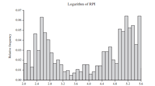
2.2 Many statistical procedures perform more effectively on data that are normally distributed, or at least are symmetric and not excessively kurtotic (fat-tailed), and where the mean and variance are approximately constant. Observed time series frequently require some form of transformation before they exhibit these distributional properties, for in their “raw” form they are often asymmetric. For example, if a series is only able to take positive (or at least nonnegative) values, then its distribution will usually be skewed to the right, because although there is a natural lower bound to the data, often zero, no upper bound exists and the values are able to “stretch out,” possibly to infinity. In this case a simple and popular transformation is to take logarithms, usually to the base $e$ (natural logarithms).
2.3 Fig. $2.1$ displays histograms of the levels and logarithms of the monthly UK retail price index (RPI) series plotted in Fig. 1.7. Taking logarithms clearly reduces the extreme right-skewness found in the levels, but it certainly does not induce normality, for the distribution of the logarithms is distinctively bimodal.
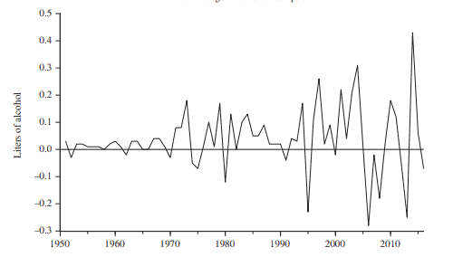
The reason for this is clearly seen in Fig. 2.2, which shows a time series plot of the logarithms of the RPI. The central part of the distribution, which has the lower relative frequency, is transited swiftly during the 1970 s, as this was a decade of high inflation characterized by the steepness of the slope of the series during this period.
Clearly, transforming to logarithms does not induce stationarity, but on comparing Fig. $2.2$ with Fig. 1.7, taking logarithms does “straighten out” the trend, at least to the extent that the periods before 1970 and after 1980 are both approximately linear with roughly the same slope. ${ }^1$ Taking logarithms also stabilizes the variance. Fig. $2.3$ plots the ratio of cumulative standard deviations, $s_i(\mathrm{RPI}) / s_i(\log \mathrm{RPI})$, defined using (1.2) and (1.3) as:
$$
s_i^2(x)=i^{-1} \sum_{t=1}^i\left(x_t-\bar{x}i\right)^2 \quad \bar{x}_i=i^{-1} \sum{t=1}^i x_t
$$
统计代写|时间序列分析代写Time-Series Analysis代考|STATIONARITY INDUCING TRANSFORMATIONS
2.9 A simple stationarity transformation is to take successive differences of a series, on defining the first-difference of $x_t$ as $\nabla x_t=x_t-x_{t-1}$. Fig. $2.6$ shows the first-differences of the wine and spirits consumption series plotted in Fig. 1.6, that is, the annual changes in consumption. The trends in both series have been eradicated by this transformation and, as will be shown in Chapter 4, ARIMA Models for Nonstationary Time Series, differencing has a lot to recommend it both practically and theoretically for transforming a nonstationary series to stationarity.
First-differencing may, on some occasions, be insufficient to induce stationarity and further differencing may be required. Fig. $2.7$ shows successive temperature readings on a chemical process, this being Series $\mathrm{C}$ of Box and Jenkins (1970). The top panel shows observed temperatures. These display a distinctive form of nonstationarity, in which there are almost random switches in trend and changes in level. Although first differencing (shown as the middle panel) mitigates these switches and changes, it by no means eliminates them; second-differences are required to achieve this, as shown in the bottom panel.
2.10 Some caution is required when taking higher-order differences. The second-differences shown in Fig. $2.7$ are defined as the first-difference of the first-difference, that is, $\nabla \nabla x_t=\nabla^2 x_t$. To provide an explicit expression for second-differences, it is convenient to introduce the lag operator $B$, defined such that $B^j x_t \equiv x_{t-j}$, so that:
$$
\nabla x_t=x_t-x_{t-1}=x_t-B x_t=(1-B) x_t
$$
Consequently:
$$
\nabla^2 x_t=(1-B)^2 x_t=\left(1-2 B+B^2\right) x_t=x_t-2 x_{t-1}+x_{t-2}
$$
which is clearly not the same as $x_t-x_{t-2}=\nabla_2 x_t$, the two-period difference, where the notation $\nabla_j=1-B^j$ for the taking of $j$-period differences has been introduced. The distinction between the two is clearly demonstrated in Fig. $2.8$, where second- and two-period differences of Series $\mathrm{C}$ are displayed.
时间序列分析代考
统计代写|时间序列分析代写Time-Series Analysis代考|DISTRIBUTIONAL TRANSFORMATIONS
$2.2$ 许多统计程序对正态分布的数据执行更有效,或者至少是对称的且没有过度峰态 (肥尾),并且均值和方差近 似为常数。观察到的时间序列在表现出这些分布特性之前经常需要某种形式的转换,因为它们的“原始”形式通常是 不对称的。例如,如果一个序列只能取正值 (或至少是非负值),那么它的分布通常会向右倾斜,因为虽然数据有 一个自然的下限,通常为零,但不存在上限并且这些值能够“延伸”到无穷大。在这种情况下,一个简单而流行的变 换是取对数,通常是底数e(自然对数)。
$2.3$ 图。2.1显示图 $1.7$ 中绘制的每月英国零售价格指数 (RPI) 系列水平和对数的直方图。取对数明显减少了水平中 发现的极端右偏度,但它肯定不会导致正态性,因为对数的分布明显是双峰的。
其原因在图 $2.2$ 中清晰可见,该图显示了 RPI 对数的时间序列图。分布的中心部分具有较低的相对频率,在 1970 年代迅速过渡,因为这是一个高通胀的十年,其特征是该期间序列斜率的陡峭。
显然,转换为对数并不会导致平稳性,而是比较图 1。2.2对于图 1.7,取对数确实“拉直”了趋势,至少在 1970 年 之前和 1980 年之后的时期都近似线性,斜率大致相同。 ${ }^1$ 取对数也可以稳定方差。如图。2.3绘制累积标准偏差的 比率, $s_i(\mathrm{RPI}) / s_i(\log \mathrm{RPI})$ ,使用 (1.2) 和 (1.3) 定义为:
$$
s_i^2(x)=i^{-1} \sum_{t=1}^i\left(x_t-\bar{x} i\right)^2 \quad \bar{x}_i=i^{-1} \sum t=1^i x_t
$$
统计代写|时间序列分析代写Time-Series Analysis代考|STATIONARITY INDUCING TRANSFORMATIONS
$2.9$ 一个简单的平稳性变换是对一个系列的连续差分,定义一阶差分 $x_t$ 作为 $\nabla x_t=x_t-x_{t-1}$. 如图。 $2.6$ 显示了 图 $1.6$ 中绘制的葡萄酒和烈酒消费系列的一阶差分,即消费的年度变化。这两个序列的趋势已经被这种转换消除 了,正如将在第 4 章,非平稳时间序列的 ARIMA 模型中展示的那样,差分对于将非平稳序列转换为平稳有很多实 际和理论上的建议。
在某些情况下,一阶差分可能不足以诱导平稳性,可能需要进一步差分。如图。2.7显示化学过程的连续温度读 数,这是系列CBox 和 Jenkins (1970)。顶部面板显示观察到的温度。这些表现出一种独特的非平稳性形式,其中 趋势和水平变化几乎是随机的。虽然一阶差分(显示为中间面板)减轻了这些转换和变化,但它绝不会消除它们; 实现这一点需要第二个差异,如底部面板所示。
$2.10$ 取高阶差分时需要小心。二次差分如图所示。 $2.7$ 被定义为一阶差分的一阶差分,即 $\nabla \nabla x_t=\nabla^2 x_t$. 为了提 供二阶差分的显式表达式,引入滞后算子很方便 $B$ ,定义为 $B^j x_t \equiv x_{t-j}$ ,以便:
$$
\nabla x_t=x_t-x_{t-1}=x_t-B x_t=(1-B) x_t
$$
最后:
$$
\nabla^2 x_t=(1-B)^2 x_t=\left(1-2 B+B^2\right) x_t=x_t-2 x_{t-1}+x_{t-2}
$$
这显然不一样 $x_t-x_{t-2}=\nabla_2 x_t$ ,两个周期的差异,其中符号 $\nabla_j=1-B^j$ 为采取 $j$-期间差异已被引入。两 者之间的区别在图 1 中清楚地显示出来。2.8,其中 Series 的第二个和两个周期的差异C被显示。

统计代写请认准statistics-lab™. statistics-lab™为您的留学生涯保驾护航。
金融工程代写
金融工程是使用数学技术来解决金融问题。金融工程使用计算机科学、统计学、经济学和应用数学领域的工具和知识来解决当前的金融问题,以及设计新的和创新的金融产品。
非参数统计代写
非参数统计指的是一种统计方法,其中不假设数据来自于由少数参数决定的规定模型;这种模型的例子包括正态分布模型和线性回归模型。
广义线性模型代考
广义线性模型(GLM)归属统计学领域,是一种应用灵活的线性回归模型。该模型允许因变量的偏差分布有除了正态分布之外的其它分布。
术语 广义线性模型(GLM)通常是指给定连续和/或分类预测因素的连续响应变量的常规线性回归模型。它包括多元线性回归,以及方差分析和方差分析(仅含固定效应)。
有限元方法代写
有限元方法(FEM)是一种流行的方法,用于数值解决工程和数学建模中出现的微分方程。典型的问题领域包括结构分析、传热、流体流动、质量运输和电磁势等传统领域。
有限元是一种通用的数值方法,用于解决两个或三个空间变量的偏微分方程(即一些边界值问题)。为了解决一个问题,有限元将一个大系统细分为更小、更简单的部分,称为有限元。这是通过在空间维度上的特定空间离散化来实现的,它是通过构建对象的网格来实现的:用于求解的数值域,它有有限数量的点。边界值问题的有限元方法表述最终导致一个代数方程组。该方法在域上对未知函数进行逼近。[1] 然后将模拟这些有限元的简单方程组合成一个更大的方程系统,以模拟整个问题。然后,有限元通过变化微积分使相关的误差函数最小化来逼近一个解决方案。
tatistics-lab作为专业的留学生服务机构,多年来已为美国、英国、加拿大、澳洲等留学热门地的学生提供专业的学术服务,包括但不限于Essay代写,Assignment代写,Dissertation代写,Report代写,小组作业代写,Proposal代写,Paper代写,Presentation代写,计算机作业代写,论文修改和润色,网课代做,exam代考等等。写作范围涵盖高中,本科,研究生等海外留学全阶段,辐射金融,经济学,会计学,审计学,管理学等全球99%专业科目。写作团队既有专业英语母语作者,也有海外名校硕博留学生,每位写作老师都拥有过硬的语言能力,专业的学科背景和学术写作经验。我们承诺100%原创,100%专业,100%准时,100%满意。
随机分析代写
随机微积分是数学的一个分支,对随机过程进行操作。它允许为随机过程的积分定义一个关于随机过程的一致的积分理论。这个领域是由日本数学家伊藤清在第二次世界大战期间创建并开始的。
时间序列分析代写
随机过程,是依赖于参数的一组随机变量的全体,参数通常是时间。 随机变量是随机现象的数量表现,其时间序列是一组按照时间发生先后顺序进行排列的数据点序列。通常一组时间序列的时间间隔为一恒定值(如1秒,5分钟,12小时,7天,1年),因此时间序列可以作为离散时间数据进行分析处理。研究时间序列数据的意义在于现实中,往往需要研究某个事物其随时间发展变化的规律。这就需要通过研究该事物过去发展的历史记录,以得到其自身发展的规律。
回归分析代写
多元回归分析渐进(Multiple Regression Analysis Asymptotics)属于计量经济学领域,主要是一种数学上的统计分析方法,可以分析复杂情况下各影响因素的数学关系,在自然科学、社会和经济学等多个领域内应用广泛。
MATLAB代写
MATLAB 是一种用于技术计算的高性能语言。它将计算、可视化和编程集成在一个易于使用的环境中,其中问题和解决方案以熟悉的数学符号表示。典型用途包括:数学和计算算法开发建模、仿真和原型制作数据分析、探索和可视化科学和工程图形应用程序开发,包括图形用户界面构建MATLAB 是一个交互式系统,其基本数据元素是一个不需要维度的数组。这使您可以解决许多技术计算问题,尤其是那些具有矩阵和向量公式的问题,而只需用 C 或 Fortran 等标量非交互式语言编写程序所需的时间的一小部分。MATLAB 名称代表矩阵实验室。MATLAB 最初的编写目的是提供对由 LINPACK 和 EISPACK 项目开发的矩阵软件的轻松访问,这两个项目共同代表了矩阵计算软件的最新技术。MATLAB 经过多年的发展,得到了许多用户的投入。在大学环境中,它是数学、工程和科学入门和高级课程的标准教学工具。在工业领域,MATLAB 是高效研究、开发和分析的首选工具。MATLAB 具有一系列称为工具箱的特定于应用程序的解决方案。对于大多数 MATLAB 用户来说非常重要,工具箱允许您学习和应用专业技术。工具箱是 MATLAB 函数(M 文件)的综合集合,可扩展 MATLAB 环境以解决特定类别的问题。可用工具箱的领域包括信号处理、控制系统、神经网络、模糊逻辑、小波、仿真等。