如果你也在 怎样代写时间序列分析Time-Series Analysis这个学科遇到相关的难题,请随时右上角联系我们的24/7代写客服。
时间序列分析是分析在一个时间间隔内收集的一系列数据点的具体方式。在时间序列分析中,分析人员在设定的时间段内以一致的时间间隔记录数据点,而不仅仅是间歇性或随机地记录数据点。
statistics-lab™ 为您的留学生涯保驾护航 在代写时间序列分析Time-Series Analysis方面已经树立了自己的口碑, 保证靠谱, 高质且原创的统计Statistics代写服务。我们的专家在代写时间序列分析Time-Series Analysis代写方面经验极为丰富,各种代写时间序列分析Time-Series Analysis相关的作业也就用不着说。
我们提供的时间序列分析Time-Series Analysis及其相关学科的代写,服务范围广, 其中包括但不限于:
- Statistical Inference 统计推断
- Statistical Computing 统计计算
- Advanced Probability Theory 高等概率论
- Advanced Mathematical Statistics 高等数理统计学
- (Generalized) Linear Models 广义线性模型
- Statistical Machine Learning 统计机器学习
- Longitudinal Data Analysis 纵向数据分析
- Foundations of Data Science 数据科学基础
统计代写|时间序列分析代写Time-Series Analysis代考|STATIONARITY INDUCING TRANSFORMATIONS
2.9 A simple stationarity transformation is to take successive differences of a series, on defining the first-difference of $x_t$ as $\nabla x_t=x_t-x_{t-1}$. Fig. $2.6$ shows the first-differences of the wine and spirits consumption series plotted in Fig. 1.6, that is, the annual changes in consumption. The trends in both series have been eradicated by this transformation and, as will be shown in Chapter 4, ARIMA Models for Nonstationary Time Series, differencing has a lot to recommend it both practically and theoretically for transforming a nonstationary series to stationarity.
First-differencing may, on some occasions, be insufficient to induce stationarity and further differencing may be required. Fig. $2.7$ shows successive temperature readings on a chemical process, this being Series $\mathrm{C}$ of Box and Jenkins (1970). The top panel shows observed temperatures. These display a distinctive form of nonstationarity, in which there are almost random switches in trend and changes in level. Although first differencing (shown as the middle panel) mitigates these switches and changes, it by no means eliminates them; second-differences are required to achieve this, as shown in the bottom panel.
2.10 Some caution is required when taking higher-order differences. The second-differences shown in Fig. $2.7$ are defined as the first-difference of the first-difference, that is, $\nabla \nabla x_t=\nabla^2 x_t$. To provide an explicit expression for second-differences, it is convenient to introduce the lag operator $B$, defined such that $B^i x_t \equiv x_{t-j}$, so that:
$$
\nabla x_t=x_t-x_{t-1}=x_t-B x_t=(1-B) x_t
$$
Consequently:
$$
\nabla^2 x_t=(1-B)^2 x_t=\left(1-2 B+B^2\right) x_t=x_t-2 x_{t-1}+x_{t-2}
$$
which is clearly not the same as $x_t-x_{t-2}=\nabla_2 x_t$, the two-period difference, where the notation $\nabla_j=1-B^j$ for the taking of $j$-period differences has been introduced. The distinction between the two is clearly demonstrated in Fig. 2.8, where second- and two-period differences of Series $\mathrm{C}$ are displayed.
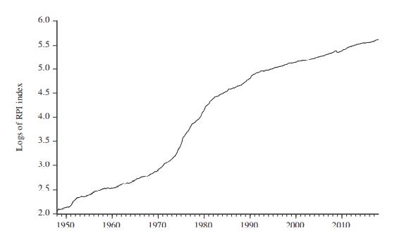
2.11 For some time series, interpretation can be made easier hy taking proportional or percentage changes rather than simple differences, that is, transforming by $\nabla x_t / x_{t-1}$ or $100 \nabla x_t / x_{t-1}$. For financial time series these are typically referred to as the return. Fig. $2.9$ plots the monthly price of gold and its percentage return from 1980 to 2017 .
统计代写|时间序列分析代写Time-Series Analysis代考|DECOMPOSING A TIME SERIES AND SMOOTHING TRANSFORMATIONS
2.17 WMAs may also arise when a simple MA with an even number of terms is used but centering is required. For example, a four-term MA may be defined as:
$$
\mathrm{MA}{t-1 / 2}(4)=\frac{1}{4}\left(x{t-2}+x_{t-1}+x_t+x_{t+1}\right)
$$
where the notation makes clear that the “central” date to which the MA relates to is a noninteger, being halfway between $t-1$ and $t$, that is, $t-(1 / 2)$, but of course $x_{t-(1 / 2)}$ does not exist and the centering property is lost. At $t+1$, however, the MA is:
$$
\operatorname{MA}{t+(1 / 2)}(4)=\frac{1}{4}\left(x{t-1}+x_t+x_{t+1}+x_{t+2}\right)
$$
which has a central date of $t+(1 / 2)$. Taking the average of these two simple MAs produces a weighted MA centered on the average of $t-(1 / 2)$ and $t+(1 / 2)$, which is, of course, $t$ :
$$
\mathrm{WMA}t(5)=\frac{1}{8} x{t-2}+\frac{1}{4} x_{t-1}+\frac{1}{4} x_t+\frac{1}{4} x_{t+1}+\frac{1}{8} x_{t+2}
$$
This is an example of (2.9) with $n=2$ and where there are “half-weights” on the two extreme observations of the MA.
2.18 Fig. $2.12$ plots two simple MAs for the daily observations on the $\$-£$ exchange rate shown in Fig. 1.5. The centered $\operatorname{MA}(251)$ has a span of approximately one year, while the backward looking one-sided MA(60) has a span stretching back over the last three months (5-day working weeks and 20-day working months being assumed here). Naturally, the former MA is much smoother, missing out on the sharper peaks and troughs captured by the latter, but reproducing the longer-term undulations of the exchange rate, known as “long swings.” It also loses the last 125 days (approximately 6 months), which might be regarded as a drawback if recent movements are thought to be of special importance.
2.19 Weighted MAs lie behind many of the trend filters that have been proposed over the years and which will be introduced in Chapter 8, Unobserved Component Models, Signal Extraction, and Filters: see Mills (2011, chapter 10) for a historical discussion. Fig. $2.13$ shows the global temperature series originally plotted in Fig. $1.8$ with a popular trend filter, known as the Hodrick-Prescott (H-P) filter, superimposed. Details of this filter are provided in $\$ \$ 8.13-8.18$, it being a symmetric weighted MA with end-point corrections that allow the filter to be computed right up to the end of the sample, thus avoiding any loss of observations. This is important here, because global temperatures are quite volatile and extracting the recent trend is essential for providing an indication of the current extent of any global warming. The weights of the MA depend on choosing a value for the smoothing parameter: here a large value has been chosen to produce a relatively “smooth trend” that focuses on the longer run movements in temperature.
时间序列分析代考
统计代写|时间序列分析代写Time-Series Analysis代考| stationary arity induced transformation
. txt
一个简单的平稳性变换是取一个级数的连续差分,将$x_t$的一阶差分定义为$\nabla x_t=x_t-x_{t-1}$。图$2.6$显示了图1.6中绘制的葡萄酒和烈酒消费序列的一阶差异,即消费的年度变化。这两个序列中的趋势都被这种转换消除了,正如第4章“非平稳时间序列的ARIMA模型”所示,差分法在将非平稳序列转换为平稳序列的实践和理论上都有很大的可取之处
在某些情况下,一阶差分可能不足以诱导平稳,可能需要进一步差分。图$2.7$显示了化学过程的连续温度读数,这是Box和Jenkins(1970)的$\mathrm{C}$系列。上面的面板显示了观测到的温度。它们表现出一种独特的非平稳形式,其中趋势和水平的变化几乎是随机的开关。尽管第一个差异(如中间面板所示)缓解了这些切换和变化,但它绝不能消除它们;
2.10在取高阶差分时需要谨慎。图$2.7$所示的二次差分定义为第一次差分的第一次差分,即$\nabla \nabla x_t=\nabla^2 x_t$。为了提供二次差的显式表达式,可以方便地引入滞后算符$B$,它被定义为$B^i x_t \equiv x_{t-j}$,从而:
$$
\nabla x_t=x_t-x_{t-1}=x_t-B x_t=(1-B) x_t
$$
因此:
$$
\nabla^2 x_t=(1-B)^2 x_t=\left(1-2 B+B^2\right) x_t=x_t-2 x_{t-1}+x_{t-2}
$$
,这显然与两个周期差的$x_t-x_{t-2}=\nabla_2 x_t$不同,这里引入了用于取$j$ -周期差的符号$\nabla_j=1-B^j$。这两者之间的区别如图2.8所示,其中显示了系列$\mathrm{C}$的第二个和两个周期的差异。对于某些时间序列,通过采用比例或百分比的变化而不是简单的差异,即通过$\nabla x_t / x_{t-1}$或$100 \nabla x_t / x_{t-1}$进行转换,可以使解释更容易。对于金融时间序列,这通常被称为收益。图$2.9$绘制了1980 – 2017年黄金月度价格及其百分比回报率
统计代写|时间序列分析代写时间序列分析代考|分解时间序列和平滑转换
当使用偶数个术语的简单MA但需要定心时,也可能出现wma。例如,一个四项的MA可以定义为:
$$
\mathrm{MA}{t-1 / 2}(4)=\frac{1}{4}\left(x{t-2}+x_{t-1}+x_t+x_{t+1}\right)
$$
,其中符号清楚地表明,MA所涉及的“中心”日期是一个非整数,位于$t-1$和$t$的中间,即$t-(1 / 2)$,但是当然$x_{t-(1 / 2)}$不存在,中心属性丢失。但是在$t+1$, MA是:
$$
\operatorname{MA}{t+(1 / 2)}(4)=\frac{1}{4}\left(x{t-1}+x_t+x_{t+1}+x_{t+2}\right)
$$
,它的中心日期是$t+(1 / 2)$。取这两个简单的MAs的平均值会产生一个以$t-(1 / 2)$和$t+(1 / 2)$的平均值为中心的加权MA,当然,这是$t$:
$$
\mathrm{WMA}t(5)=\frac{1}{8} x{t-2}+\frac{1}{4} x_{t-1}+\frac{1}{4} x_t+\frac{1}{4} x_{t+1}+\frac{1}{8} x_{t+2}
$$
这是(2.9)的一个例子,$n=2$,在MA的两个极端观测值上有“半权值”。
2.18图$2.12$绘制了图1.5中所示$\$-£$汇率每日观测值的两个简单MA。中间的$\operatorname{MA}(251)$的跨度大约为一年,而向后看的单侧MA(60)的跨度可以追溯到过去的三个月(这里假设为5天工作周和20天工作月)。自然,前一个MA要平滑得多,没有后者捕捉到的尖峰和波谷,而是再现了汇率的长期波动,即“长期波动”。它也失去了过去的125天(大约6个月),如果最近的移动被认为是特别重要的,这可能被视为一个缺点。加权MAs隐藏在许多趋势过滤器的背后,这些趋势过滤器多年来一直被提出,将在第8章,未观测组件模型,信号提取和过滤器中介绍:参见Mills(2011,第10章)进行历史讨论。图$2.13$显示了最初绘制在图$1.8$中的全球温度序列,其中叠加了一个流行的趋势滤波器,即Hodrick-Prescott (hp)滤波器。该滤波器的详细信息在$\$ \$ 8.13-8.18$中提供,它是一个带有端点修正的对称加权MA,允许在样本结束前计算滤波器,从而避免任何观测损失。这一点在这里很重要,因为全球温度是非常不稳定的,提取最近的趋势对于提供任何全球变暖当前程度的指示是至关重要的。MA的权重取决于为平滑参数选择一个值:这里选择了一个较大的值,以产生一个相对“平滑的趋势”,关注温度的长期运动

统计代写请认准statistics-lab™. statistics-lab™为您的留学生涯保驾护航。
金融工程代写
金融工程是使用数学技术来解决金融问题。金融工程使用计算机科学、统计学、经济学和应用数学领域的工具和知识来解决当前的金融问题,以及设计新的和创新的金融产品。
非参数统计代写
非参数统计指的是一种统计方法,其中不假设数据来自于由少数参数决定的规定模型;这种模型的例子包括正态分布模型和线性回归模型。
广义线性模型代考
广义线性模型(GLM)归属统计学领域,是一种应用灵活的线性回归模型。该模型允许因变量的偏差分布有除了正态分布之外的其它分布。
术语 广义线性模型(GLM)通常是指给定连续和/或分类预测因素的连续响应变量的常规线性回归模型。它包括多元线性回归,以及方差分析和方差分析(仅含固定效应)。
有限元方法代写
有限元方法(FEM)是一种流行的方法,用于数值解决工程和数学建模中出现的微分方程。典型的问题领域包括结构分析、传热、流体流动、质量运输和电磁势等传统领域。
有限元是一种通用的数值方法,用于解决两个或三个空间变量的偏微分方程(即一些边界值问题)。为了解决一个问题,有限元将一个大系统细分为更小、更简单的部分,称为有限元。这是通过在空间维度上的特定空间离散化来实现的,它是通过构建对象的网格来实现的:用于求解的数值域,它有有限数量的点。边界值问题的有限元方法表述最终导致一个代数方程组。该方法在域上对未知函数进行逼近。[1] 然后将模拟这些有限元的简单方程组合成一个更大的方程系统,以模拟整个问题。然后,有限元通过变化微积分使相关的误差函数最小化来逼近一个解决方案。
tatistics-lab作为专业的留学生服务机构,多年来已为美国、英国、加拿大、澳洲等留学热门地的学生提供专业的学术服务,包括但不限于Essay代写,Assignment代写,Dissertation代写,Report代写,小组作业代写,Proposal代写,Paper代写,Presentation代写,计算机作业代写,论文修改和润色,网课代做,exam代考等等。写作范围涵盖高中,本科,研究生等海外留学全阶段,辐射金融,经济学,会计学,审计学,管理学等全球99%专业科目。写作团队既有专业英语母语作者,也有海外名校硕博留学生,每位写作老师都拥有过硬的语言能力,专业的学科背景和学术写作经验。我们承诺100%原创,100%专业,100%准时,100%满意。
随机分析代写
随机微积分是数学的一个分支,对随机过程进行操作。它允许为随机过程的积分定义一个关于随机过程的一致的积分理论。这个领域是由日本数学家伊藤清在第二次世界大战期间创建并开始的。
时间序列分析代写
随机过程,是依赖于参数的一组随机变量的全体,参数通常是时间。 随机变量是随机现象的数量表现,其时间序列是一组按照时间发生先后顺序进行排列的数据点序列。通常一组时间序列的时间间隔为一恒定值(如1秒,5分钟,12小时,7天,1年),因此时间序列可以作为离散时间数据进行分析处理。研究时间序列数据的意义在于现实中,往往需要研究某个事物其随时间发展变化的规律。这就需要通过研究该事物过去发展的历史记录,以得到其自身发展的规律。
回归分析代写
多元回归分析渐进(Multiple Regression Analysis Asymptotics)属于计量经济学领域,主要是一种数学上的统计分析方法,可以分析复杂情况下各影响因素的数学关系,在自然科学、社会和经济学等多个领域内应用广泛。
MATLAB代写
MATLAB 是一种用于技术计算的高性能语言。它将计算、可视化和编程集成在一个易于使用的环境中,其中问题和解决方案以熟悉的数学符号表示。典型用途包括:数学和计算算法开发建模、仿真和原型制作数据分析、探索和可视化科学和工程图形应用程序开发,包括图形用户界面构建MATLAB 是一个交互式系统,其基本数据元素是一个不需要维度的数组。这使您可以解决许多技术计算问题,尤其是那些具有矩阵和向量公式的问题,而只需用 C 或 Fortran 等标量非交互式语言编写程序所需的时间的一小部分。MATLAB 名称代表矩阵实验室。MATLAB 最初的编写目的是提供对由 LINPACK 和 EISPACK 项目开发的矩阵软件的轻松访问,这两个项目共同代表了矩阵计算软件的最新技术。MATLAB 经过多年的发展,得到了许多用户的投入。在大学环境中,它是数学、工程和科学入门和高级课程的标准教学工具。在工业领域,MATLAB 是高效研究、开发和分析的首选工具。MATLAB 具有一系列称为工具箱的特定于应用程序的解决方案。对于大多数 MATLAB 用户来说非常重要,工具箱允许您学习和应用专业技术。工具箱是 MATLAB 函数(M 文件)的综合集合,可扩展 MATLAB 环境以解决特定类别的问题。可用工具箱的领域包括信号处理、控制系统、神经网络、模糊逻辑、小波、仿真等。