如果你也在 怎样代写时间序列分析Time-Series Analysis这个学科遇到相关的难题,请随时右上角联系我们的24/7代写客服。
时间序列分析是分析在一个时间间隔内收集的一系列数据点的具体方式。在时间序列分析中,分析人员在设定的时间段内以一致的时间间隔记录数据点,而不仅仅是间歇性或随机地记录数据点。
statistics-lab™ 为您的留学生涯保驾护航 在代写时间序列分析Time-Series Analysis方面已经树立了自己的口碑, 保证靠谱, 高质且原创的统计Statistics代写服务。我们的专家在代写时间序列分析Time-Series Analysis代写方面经验极为丰富,各种代写时间序列分析Time-Series Analysis相关的作业也就用不着说。
我们提供的时间序列分析Time-Series Analysis及其相关学科的代写,服务范围广, 其中包括但不限于:
- Statistical Inference 统计推断
- Statistical Computing 统计计算
- Advanced Probability Theory 高等概率论
- Advanced Mathematical Statistics 高等数理统计学
- (Generalized) Linear Models 广义线性模型
- Statistical Machine Learning 统计机器学习
- Longitudinal Data Analysis 纵向数据分析
- Foundations of Data Science 数据科学基础
统计代写|时间序列分析代写Time-Series Analysis代考|Prediction, Classification, and Chaos
The attractor of the dynamical systems producing $s(t)$ is contained in dimension $d_E$ which assures that there is no residual overlap of trajectories from the projection to one dimension: $s(t)$. To characterize the attractor we can call on many different notions of dimension of the set of points $\mathbf{y}(\mathrm{n})$. Each is an invariant of the dynamical system in the sense that a smooth coordinate change from those used in $y(n)$, including that involved in changing $T$, leaves these characteristic numbers unchanged. The invariance comes from the fact that each dimension estimate is a local property of the point set comprising the attractor, and smooth changes of coordinates do not alter this local property while they might change the global appearance of the attractor. These various dimensions are covered in many books, and each is interesting.
We here focus on a dynamical invariant of the attractor that also allows an estimate of dimension. The central issue is the stability of an orbit such as $\mathbf{y}(\mathrm{n})$ under perturbations to points on the trajectory. This is a familiar question associated with the stability of fixed points or limit cycles as studied in classical fields such as fluid dynamics. If one has a fixed point $x_0$ of a dynamical system in d dimension $x(t)=\left[x_1(t), x_2(t), \ldots, x_d(t)\right]$ with $x(t)$ satisfying
$$
\frac{d x(t)}{d t}=\mathbf{G}(x(t))
$$
so $\mathbf{G}\left(\mathrm{x}_0\right)=0$, then it is important to ask if state space points $x_0+\Delta x(t)$ are stable in the sense they remain near or return to $x_0$. Unstable points, where $\Delta x(t)$ grows large, are not realized in observations of a dynamical system.
统计代写|时间序列分析代写Time-Series Analysis代考|Modeling Interspike Intervals
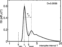
To start with a simple example for black-box modeling we consider the interspike intervals of the given neuron time series shown in Fig. 2.8. As already mentioned in Section 2.2.3 this diagram suggests an approximate description in terms of some function $\Delta t_{k+1}=g\left(\Delta t_k\right)$. The goal of (black-box) modeling is to find a function $g$ that fulfills this task in some optimal sense (to be specified). In particular, the function should have good generalization properties: not only the given time series has to be mapped correctly but also new data from the same source (not yet seen when learning the model). To achieve this (ambitious) goal overfitting has to be avoided, i.e., the model must not incorporate features of the particular realization of the given (finite!) time series. The performance of a good model does not depend on statistical features like random choice of initial conditions on a (chaotic) attractor or purely stochastic components (noise) that will not be the same for different measurements from a fixed (stationary) source or process. So the model has to be flexible enough to describe the data but should not be too complex, because then it will start to model also realization-dependent features. To determine some suitable level of complexity one may employ complexity measures and balance them with the prediction error. Another practically useful method is cross validation. The given data set is split into two parts: a learning or training set and an independent test set. The training set is used to specify the model (including parameters), and this model is then applied to the test set to evaluated its generalization properties and potential overfitting. To illustrate this point we shall fit a polynomial to the interspike intervals within a burst shown in Fig. $2.8$ (enlargement on the right-hand side). These data points are randomly split into two halves, training and test set. A polynomial of degree $m$ is fit to the training set and then used to map the test data points. For both sets of points mean squared errors are computed, called $E_{\text {train }}$ and $E_{\text {test. }}$ In Fig. $2.12$ both errors are plotted versus $m$. Increasing the degree $m$ renders our model more complex and results in a monotonically decreasing error $E_{\text {train }}$ of the training set (dashed line in Fig. 2.12). For small $m$ the error $E_{\text {test }}$ of the test set also decreases but at $m=3$ it starts to increase again, because for too complex polynomials overfitting sets in and the performance of the model on the test set deteriorates. To obtain a representative and robust evaluation of the model performance the time series has been split randomly several times in different training and test sets and the given errors are mean values of the corresponding training and test errors.
时间序列分析代考
统计代写|时间序列分析代写Time-Series Analysis代考|Prediction, Classification, and Chaos
动力系统的吸引子产生 $s(t)$ 包含在维度中 $d_E$ 这确保从投影到一维的轨迹没有残余重叠: $s(t)$. 为了表征吸引子,我们可以调用点集的许多不同维度概念 $\mathbf{y}(\mathrm{n})$. 每个都是动力系统的不变量, 因为平滑的坐标从中使用的坐标变化 $y(n)$ ,包括涉及改变的 $T$, 保留这些特征数不变。不变性 来自这样一个事实,即每个维度估计都是包含吸引子的点集的局部属性,坐标的平滑变化不会 改变这个局部属性,但它们可能会改变吸引子的全局外观。这些不同的维度在很多书中都有涉 及,每一个都很有趣。
我们在这里关注吸引子的动态不变量,它也允许估计维度。核心问题是轨道的稳定性,例如 $\mathbf{y}(\mathrm{n})$ 在对轨迹上的点的扰动下。这是与流体动力学等经典领域研究的不动点或极限环的稳定 性相关的常见问题。如果一个人有一个固定点 $x_0 \mathrm{~d}$ 维动力系统 $x(t)=\left[x_1(t), x_2(t), \ldots, x_d(t)\right]$ 和 $x(t)$ 令人满意
$$
\frac{d x(t)}{d t}=\mathbf{G}(x(t))
$$
所以 $\mathbf{G}\left(\mathrm{x}_0\right)=0$ ,那么重要的是要问状态空间是否指向 $x_0+\Delta x(t)$ 在他们保持接近或返回 的意义上是稳定的 $x_0$. 不稳定点,其中 $\Delta x(t)$ 变大,在动力系统的观察中没有意识到。
统计代写|时间序列分析代写Time-Series Analysis代考|Modeling Interspike Intervals
从一个简单的黑盒建模示例开始,我们考虑图 2.8 中所示的给定神经元时间序列的尖峰间隔。正如第 2.2.3 节中已经提到的,该图建议根据某些功能进行近似描述丁吨k+1=G(丁吨k). (黑盒)建模的目标是找到一个函数G在某种最佳意义上完成此任务(待指定)。特别是,该函数应该具有良好的泛化特性:不仅必须正确映射给定的时间序列,而且还必须正确映射来自同一来源的新数据(在学习模型时尚未看到)。为了实现这个(雄心勃勃的)目标,必须避免过度拟合,即模型不得包含给定(有限!)时间序列的特定实现的特征。一个好的模型的性能不依赖于统计特征,例如在(混沌)吸引子上随机选择初始条件或纯随机成分(噪声),这些特征对于来自固定(静止)源或过程的不同测量是不同的。所以模型必须足够灵活来描述数据但不应该太复杂,因为那时它将开始建模也依赖于实现的特征。为了确定某种合适的复杂程度,可以采用复杂性度量并将它们与预测误差进行平衡。另一个实际有用的方法是交叉验证。给定的数据集分为两部分:学习或训练集和独立的测试集。训练集用于指定模型(包括参数),然后将该模型应用于测试集以评估其泛化特性和潜在的过度拟合。为了说明这一点,我们将用多项式拟合图 1 所示的脉冲串中的尖峰间间隔。另一个实际有用的方法是交叉验证。给定的数据集分为两部分:学习或训练集和独立的测试集。训练集用于指定模型(包括参数),然后将该模型应用于测试集以评估其泛化特性和潜在的过度拟合。为了说明这一点,我们将用多项式拟合图 1 所示的脉冲串中的尖峰间间隔。另一个实际有用的方法是交叉验证。给定的数据集分为两部分:学习或训练集和独立的测试集。训练集用于指定模型(包括参数),然后将该模型应用于测试集以评估其泛化特性和潜在的过度拟合。为了说明这一点,我们将用多项式拟合图 1 所示的脉冲串中的尖峰间间隔。2.8(右侧放大)。这些数据点随机分成两半,训练集和测试集。一次多项式米适合训练集,然后用于映射测试数据点。计算两组点的均方误差,称为和火车 和和测试。 在图2.12两个错误都被绘制为米. 增加学位米使我们的模型更加复杂并导致单调递减的误差和火车 训练集(图 2.12 中的虚线)。对于小米错误和测试 测试集的也减少但在米=3它再次开始增加,因为对于太复杂的多项式,过度拟合开始并且模型在测试集上的性能恶化。为了获得对模型性能的代表性和鲁棒性评估,时间序列在不同的训练和测试集中被随机分割了几次,给定的误差是相应训练和测试误差的平均值。

统计代写请认准statistics-lab™. statistics-lab™为您的留学生涯保驾护航。
金融工程代写
金融工程是使用数学技术来解决金融问题。金融工程使用计算机科学、统计学、经济学和应用数学领域的工具和知识来解决当前的金融问题,以及设计新的和创新的金融产品。
非参数统计代写
非参数统计指的是一种统计方法,其中不假设数据来自于由少数参数决定的规定模型;这种模型的例子包括正态分布模型和线性回归模型。
广义线性模型代考
广义线性模型(GLM)归属统计学领域,是一种应用灵活的线性回归模型。该模型允许因变量的偏差分布有除了正态分布之外的其它分布。
术语 广义线性模型(GLM)通常是指给定连续和/或分类预测因素的连续响应变量的常规线性回归模型。它包括多元线性回归,以及方差分析和方差分析(仅含固定效应)。
有限元方法代写
有限元方法(FEM)是一种流行的方法,用于数值解决工程和数学建模中出现的微分方程。典型的问题领域包括结构分析、传热、流体流动、质量运输和电磁势等传统领域。
有限元是一种通用的数值方法,用于解决两个或三个空间变量的偏微分方程(即一些边界值问题)。为了解决一个问题,有限元将一个大系统细分为更小、更简单的部分,称为有限元。这是通过在空间维度上的特定空间离散化来实现的,它是通过构建对象的网格来实现的:用于求解的数值域,它有有限数量的点。边界值问题的有限元方法表述最终导致一个代数方程组。该方法在域上对未知函数进行逼近。[1] 然后将模拟这些有限元的简单方程组合成一个更大的方程系统,以模拟整个问题。然后,有限元通过变化微积分使相关的误差函数最小化来逼近一个解决方案。
tatistics-lab作为专业的留学生服务机构,多年来已为美国、英国、加拿大、澳洲等留学热门地的学生提供专业的学术服务,包括但不限于Essay代写,Assignment代写,Dissertation代写,Report代写,小组作业代写,Proposal代写,Paper代写,Presentation代写,计算机作业代写,论文修改和润色,网课代做,exam代考等等。写作范围涵盖高中,本科,研究生等海外留学全阶段,辐射金融,经济学,会计学,审计学,管理学等全球99%专业科目。写作团队既有专业英语母语作者,也有海外名校硕博留学生,每位写作老师都拥有过硬的语言能力,专业的学科背景和学术写作经验。我们承诺100%原创,100%专业,100%准时,100%满意。
随机分析代写
随机微积分是数学的一个分支,对随机过程进行操作。它允许为随机过程的积分定义一个关于随机过程的一致的积分理论。这个领域是由日本数学家伊藤清在第二次世界大战期间创建并开始的。
时间序列分析代写
随机过程,是依赖于参数的一组随机变量的全体,参数通常是时间。 随机变量是随机现象的数量表现,其时间序列是一组按照时间发生先后顺序进行排列的数据点序列。通常一组时间序列的时间间隔为一恒定值(如1秒,5分钟,12小时,7天,1年),因此时间序列可以作为离散时间数据进行分析处理。研究时间序列数据的意义在于现实中,往往需要研究某个事物其随时间发展变化的规律。这就需要通过研究该事物过去发展的历史记录,以得到其自身发展的规律。
回归分析代写
多元回归分析渐进(Multiple Regression Analysis Asymptotics)属于计量经济学领域,主要是一种数学上的统计分析方法,可以分析复杂情况下各影响因素的数学关系,在自然科学、社会和经济学等多个领域内应用广泛。
MATLAB代写
MATLAB 是一种用于技术计算的高性能语言。它将计算、可视化和编程集成在一个易于使用的环境中,其中问题和解决方案以熟悉的数学符号表示。典型用途包括:数学和计算算法开发建模、仿真和原型制作数据分析、探索和可视化科学和工程图形应用程序开发,包括图形用户界面构建MATLAB 是一个交互式系统,其基本数据元素是一个不需要维度的数组。这使您可以解决许多技术计算问题,尤其是那些具有矩阵和向量公式的问题,而只需用 C 或 Fortran 等标量非交互式语言编写程序所需的时间的一小部分。MATLAB 名称代表矩阵实验室。MATLAB 最初的编写目的是提供对由 LINPACK 和 EISPACK 项目开发的矩阵软件的轻松访问,这两个项目共同代表了矩阵计算软件的最新技术。MATLAB 经过多年的发展,得到了许多用户的投入。在大学环境中,它是数学、工程和科学入门和高级课程的标准教学工具。在工业领域,MATLAB 是高效研究、开发和分析的首选工具。MATLAB 具有一系列称为工具箱的特定于应用程序的解决方案。对于大多数 MATLAB 用户来说非常重要,工具箱允许您学习和应用专业技术。工具箱是 MATLAB 函数(M 文件)的综合集合,可扩展 MATLAB 环境以解决特定类别的问题。可用工具箱的领域包括信号处理、控制系统、神经网络、模糊逻辑、小波、仿真等。