如果你也在 怎样代写时间序列分析Time-Series Analysis这个学科遇到相关的难题,请随时右上角联系我们的24/7代写客服。
时间序列分析是分析在一个时间间隔内收集的一系列数据点的具体方式。在时间序列分析中,分析人员在设定的时间段内以一致的时间间隔记录数据点,而不仅仅是间歇性或随机地记录数据点。
statistics-lab™ 为您的留学生涯保驾护航 在代写时间序列分析Time-Series Analysis方面已经树立了自己的口碑, 保证靠谱, 高质且原创的统计Statistics代写服务。我们的专家在代写时间序列分析Time-Series Analysis代写方面经验极为丰富,各种代写时间序列分析Time-Series Analysis相关的作业也就用不着说。
我们提供的时间序列分析Time-Series Analysis及其相关学科的代写,服务范围广, 其中包括但不限于:
- Statistical Inference 统计推断
- Statistical Computing 统计计算
- Advanced Probability Theory 高等概率论
- Advanced Mathematical Statistics 高等数理统计学
- (Generalized) Linear Models 广义线性模型
- Statistical Machine Learning 统计机器学习
- Longitudinal Data Analysis 纵向数据分析
- Foundations of Data Science 数据科学基础
统计代写|时间序列分析代写Time-Series Analysis代考|Seasonal ARIMA Modeling of Beer Sales
The SACF for the $\nabla \nabla^4$ transformation of beer sales shown in Fig. $9.3$ has $r_1=-0.56, r_2=-0.03, r_3=0.44, r_4=-0.65$, and $r_5=0.30$. Since $r_2 \approx 0$ and $r_1 r_4=0.36$, these first five sample autocorrelations are, within reasonable sampling limits, consistent with the ACF of an $\operatorname{ARIMA}(0,1,1)(0,1,1)4$ airline model. Using (9.7) the standard error of the sample autocorrelations for lags greater than 5 is calculated to be $0.20$. Only $r{16}$ exceeds two-standard errors, suggesting that this airline model could represent a satisfactory representation of the beer sales data. Fitting this model obtains ${ }^4$ :
$$
\nabla_1 \nabla_4 x_t=\left(1-\begin{array}{c}
0.694 \
(0.098)
\end{array}\right)\left(1-\begin{array}{c}
0.604 \
(0.110)
\end{array} B^4\right) a_t \quad \hat{\sigma}=271.9
$$
The more general seasonal ARIMA model is estimated to be:
$$
\nabla \nabla_4 x_t=\left(1-\underset{(0.072)}{0.802} B-\underset{(0.095)}{0.552} B^4+\begin{array}{c}
0.631 \
(0.098)
\end{array} B^5\right) a_t \quad \hat{\sigma}=265.0
$$
The multiplicative model imposes the nonlinear restriction $\theta_1 \theta_4+\theta_5=0$. The log-likelihoods of the two models are $-547.76$ and $-545.64$, leading to a likelihood ratio test statistic of $4.24$, which is distributed as chi-square with one degree of freedom and so is not quite significant at the $2.5 \%$ level, although a Wald test does prove to be significant.
Using $\theta=0.7$ and $\Theta=0.6$ for simplicity, then the $\psi$-weights of the airline model are given, in general, by:
$$
\begin{gathered}
\psi_{4 r+1}=\psi_{4 r+2}=\psi_{4(r+1)-1}=0.3(r+1-0.6 r)=0.3+0.12 r \
\psi_{4(r+1)}=0.3(r+1-0.6 r)+0.4=0.7+0.12 r
\end{gathered}
$$
Thus,
$$
\begin{aligned}
&\psi_1=\psi_2=\psi_3=0.3 \
&\psi_4=0.7 \
&\psi_5=\psi_6=\psi_7=0.42 \
&\psi_8=0.82 \
&\psi_9=\psi_{10}=\psi_{11}=0.54, \text { etc. }
\end{aligned}
$$
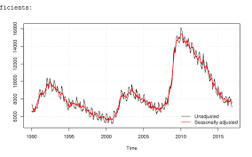
统计代写|时间序列分析代写Time-Series Analysis代考|SEASONAL ADJUSTMENT
9.13 In $\S 2.16$ we introduced a decomposition of an observed time series into trend, seasonal, and irregular (or noise) components, focusing attention on estimating the seasonal component and then eliminating it to provide a seasonally adjusted series. Extending the notation introduced in (8.1), this implicit UC decomposition can be written as
$$
x_t=z_t+s_t+u_t
$$
where the additional seasonal component $s_t$ is assumed to be independent of both $z_t$ and $u_t$. On obtaining an estimate of the seasonal component, $\hat{s}_t$, the seasonally adjusted series can then be defined as $x_t^a=x_t-\hat{s}_t$.
9.14 An important question is why we would wish to remove the seasonal component, rather than modeling it as an integral part of the stochastic process generating the data, as in fitting a seasonal ARIMA model, for example. A commonly held view is that the ability to recognize, interpret, or react to important nonseasonal movements in a series, such as turning points and other cyclical events, emerging patterns, or unexpected occurrences for which potential causes might be sought, may well be hindered by the presence of seasonal movements. Consequently, seasonal adjustment is carried out to simplify data so that they may be more easily interpreted by “statistically unsophisticated” users without this simplification being accompanied by too large a loss of information.
This qualifier is important because it requires that the seasonal adjustment procedure does not result in a “significant” loss of information. Although the moving average method introduced in $\$ 2.16$ is both intuitively and computationally simple, it may not be the best available method. Historically, seasonal adjustment methods have been categorized as either empirically- or model-based. The moving average method falls into the former category, as are the methods developed by statistical agencies, such as the sequence of procedures developed by the United States Bureau of the Census, the latest incarnation being known as X-13. Model-based methods employ signal extraction techniques based on ARIMA models fitted either to the observed series or to its components. The most popular of these methods is known as TRAMO/SEATS: see Gómez and Maravall (1996) and Mills (2013b). The distinction between empirical and model-based methods is, however, becoming blurred as X-13 also uses ARIMA models in its computations. ${ }^6$
时间序列分析代考
统计代写|时间序列分析代写时间序列分析代考|啤酒销售的季节性ARIMA建模
图$9.3$所示的啤酒销售$\nabla \nabla^4$转型的SACF有$r_1=-0.56, r_2=-0.03, r_3=0.44, r_4=-0.65$,和$r_5=0.30$。从$r_2 \approx 0$和$r_1 r_4=0.36$开始,在合理的抽样范围内,这前五个样本自相关性与$\operatorname{ARIMA}(0,1,1)(0,1,1)4$航空公司模型的ACF一致。使用(9.7)计算滞后大于5的样本自相关的标准误差为$0.20$。只有$r{16}$超过了两个标准误差,这表明这个航空公司模型可以代表一个令人满意的啤酒销售数据的表示。拟合该模型得到${ }^4$:
$$
\nabla_1 \nabla_4 x_t=\left(1-\begin{array}{c}
0.694 \
(0.098)
\end{array}\right)\left(1-\begin{array}{c}
0.604 \
(0.110)
\end{array} B^4\right) a_t \quad \hat{\sigma}=271.9
$$
更一般的季节性ARIMA模型估计为:
$$
\nabla \nabla_4 x_t=\left(1-\underset{(0.072)}{0.802} B-\underset{(0.095)}{0.552} B^4+\begin{array}{c}
0.631 \
(0.098)
\end{array} B^5\right) a_t \quad \hat{\sigma}=265.0
$$
乘法模型施加了非线性约束$\theta_1 \theta_4+\theta_5=0$。两个模型的对数似然是$-547.76$和$-545.64$,导致了$4.24$的似然比检验统计量,它以一个自由度的卡方分布,因此在$2.5 \%$水平上不太显著,尽管Wald检验确实证明显著。
为了简单起见,使用$\theta=0.7$和$\Theta=0.6$,那么航空公司模型的$\psi$ -权重一般由:
$$
\begin{gathered}
\psi_{4 r+1}=\psi_{4 r+2}=\psi_{4(r+1)-1}=0.3(r+1-0.6 r)=0.3+0.12 r \
\psi_{4(r+1)}=0.3(r+1-0.6 r)+0.4=0.7+0.12 r
\end{gathered}
$$
因此,
$$
\begin{aligned}
&\psi_1=\psi_2=\psi_3=0.3 \
&\psi_4=0.7 \
&\psi_5=\psi_6=\psi_7=0.42 \
&\psi_8=0.82 \
&\psi_9=\psi_{10}=\psi_{11}=0.54, \text { etc. }
\end{aligned}
$$
统计代写|时间序列分析代写时间序列分析代考|季节性调整
9.13 In $\S 2.16$ 我们将观察到的时间序列分解为趋势、季节和不规则(或噪声)成分,重点关注估计季节成分,然后消除它,以提供季节性调整的序列。扩展(8.1)中介绍的符号,这个隐式UC分解可以写成
$$
x_t=z_t+s_t+u_t
$$
其中附加的季节性成分 $s_t$ 是独立于两者的吗 $z_t$ 和 $u_t$。在得到季节成分的估计后, $\hat{s}_t$,则季节性调整序列可定义为 $x_t^a=x_t-\hat{s}_t$一个重要的问题是,为什么我们希望删除季节性成分,而不是将其建模为生成数据的随机过程的一个整体部分,例如,在拟合季节性ARIMA模型时。一种普遍的观点认为,识别、解释或对一系列重要的非季节性运动(如转折点和其他周期性事件、新出现的模式或可能寻找潜在原因的意外事件)作出反应的能力很可能会受到季节性运动的存在的阻碍。因此,进行了季节调整,以简化数据,使“统计上不熟练”的用户可以更容易地解释这些数据,而不会伴随这种简化而造成太大的信息损失 这个限定符很重要,因为它要求季节调整过程不会导致信息的“重大”损失。虽然$\$ 2.16$中介绍的移动平均方法直观且计算简单,但它可能不是最好的可用方法。历史上,季节性调整方法被分为基于经验和基于模型的两类。移动平均方法属于前一类,由统计机构制定的方法也属于前一类,例如由美国人口普查局制定的一系列程序,其最新版本被称为X-13。基于模型的方法采用基于拟合观测序列或其组成部分的ARIMA模型的信号提取技术。这些方法中最流行的是TRAMO/SEATS:见Gómez和Maravall(1996)和Mills (2013b)。然而,经验方法和基于模型的方法之间的区别正在变得模糊,因为X-13在其计算中也使用ARIMA模型。${ }^6$

统计代写请认准statistics-lab™. statistics-lab™为您的留学生涯保驾护航。
金融工程代写
金融工程是使用数学技术来解决金融问题。金融工程使用计算机科学、统计学、经济学和应用数学领域的工具和知识来解决当前的金融问题,以及设计新的和创新的金融产品。
非参数统计代写
非参数统计指的是一种统计方法,其中不假设数据来自于由少数参数决定的规定模型;这种模型的例子包括正态分布模型和线性回归模型。
广义线性模型代考
广义线性模型(GLM)归属统计学领域,是一种应用灵活的线性回归模型。该模型允许因变量的偏差分布有除了正态分布之外的其它分布。
术语 广义线性模型(GLM)通常是指给定连续和/或分类预测因素的连续响应变量的常规线性回归模型。它包括多元线性回归,以及方差分析和方差分析(仅含固定效应)。
有限元方法代写
有限元方法(FEM)是一种流行的方法,用于数值解决工程和数学建模中出现的微分方程。典型的问题领域包括结构分析、传热、流体流动、质量运输和电磁势等传统领域。
有限元是一种通用的数值方法,用于解决两个或三个空间变量的偏微分方程(即一些边界值问题)。为了解决一个问题,有限元将一个大系统细分为更小、更简单的部分,称为有限元。这是通过在空间维度上的特定空间离散化来实现的,它是通过构建对象的网格来实现的:用于求解的数值域,它有有限数量的点。边界值问题的有限元方法表述最终导致一个代数方程组。该方法在域上对未知函数进行逼近。[1] 然后将模拟这些有限元的简单方程组合成一个更大的方程系统,以模拟整个问题。然后,有限元通过变化微积分使相关的误差函数最小化来逼近一个解决方案。
tatistics-lab作为专业的留学生服务机构,多年来已为美国、英国、加拿大、澳洲等留学热门地的学生提供专业的学术服务,包括但不限于Essay代写,Assignment代写,Dissertation代写,Report代写,小组作业代写,Proposal代写,Paper代写,Presentation代写,计算机作业代写,论文修改和润色,网课代做,exam代考等等。写作范围涵盖高中,本科,研究生等海外留学全阶段,辐射金融,经济学,会计学,审计学,管理学等全球99%专业科目。写作团队既有专业英语母语作者,也有海外名校硕博留学生,每位写作老师都拥有过硬的语言能力,专业的学科背景和学术写作经验。我们承诺100%原创,100%专业,100%准时,100%满意。
随机分析代写
随机微积分是数学的一个分支,对随机过程进行操作。它允许为随机过程的积分定义一个关于随机过程的一致的积分理论。这个领域是由日本数学家伊藤清在第二次世界大战期间创建并开始的。
时间序列分析代写
随机过程,是依赖于参数的一组随机变量的全体,参数通常是时间。 随机变量是随机现象的数量表现,其时间序列是一组按照时间发生先后顺序进行排列的数据点序列。通常一组时间序列的时间间隔为一恒定值(如1秒,5分钟,12小时,7天,1年),因此时间序列可以作为离散时间数据进行分析处理。研究时间序列数据的意义在于现实中,往往需要研究某个事物其随时间发展变化的规律。这就需要通过研究该事物过去发展的历史记录,以得到其自身发展的规律。
回归分析代写
多元回归分析渐进(Multiple Regression Analysis Asymptotics)属于计量经济学领域,主要是一种数学上的统计分析方法,可以分析复杂情况下各影响因素的数学关系,在自然科学、社会和经济学等多个领域内应用广泛。
MATLAB代写
MATLAB 是一种用于技术计算的高性能语言。它将计算、可视化和编程集成在一个易于使用的环境中,其中问题和解决方案以熟悉的数学符号表示。典型用途包括:数学和计算算法开发建模、仿真和原型制作数据分析、探索和可视化科学和工程图形应用程序开发,包括图形用户界面构建MATLAB 是一个交互式系统,其基本数据元素是一个不需要维度的数组。这使您可以解决许多技术计算问题,尤其是那些具有矩阵和向量公式的问题,而只需用 C 或 Fortran 等标量非交互式语言编写程序所需的时间的一小部分。MATLAB 名称代表矩阵实验室。MATLAB 最初的编写目的是提供对由 LINPACK 和 EISPACK 项目开发的矩阵软件的轻松访问,这两个项目共同代表了矩阵计算软件的最新技术。MATLAB 经过多年的发展,得到了许多用户的投入。在大学环境中,它是数学、工程和科学入门和高级课程的标准教学工具。在工业领域,MATLAB 是高效研究、开发和分析的首选工具。MATLAB 具有一系列称为工具箱的特定于应用程序的解决方案。对于大多数 MATLAB 用户来说非常重要,工具箱允许您学习和应用专业技术。工具箱是 MATLAB 函数(M 文件)的综合集合,可扩展 MATLAB 环境以解决特定类别的问题。可用工具箱的领域包括信号处理、控制系统、神经网络、模糊逻辑、小波、仿真等。