如果你也在 怎样代写贝叶斯分析Bayesian Analysis这个学科遇到相关的难题,请随时右上角联系我们的24/7代写客服。
贝叶斯分析,一种统计推断方法(以英国数学家托马斯-贝叶斯命名),允许人们将关于人口参数的先验信息与样本所含信息的证据相结合,以指导统计推断过程。
statistics-lab™ 为您的留学生涯保驾护航 在代写贝叶斯分析Bayesian Analysis方面已经树立了自己的口碑, 保证靠谱, 高质且原创的统计Statistics代写服务。我们的专家在代写贝叶斯分析Bayesian Analysis代写方面经验极为丰富,各种代写贝叶斯分析Bayesian Analysis相关的作业也就用不着说。
我们提供的贝叶斯分析Bayesian Analysis及其相关学科的代写,服务范围广, 其中包括但不限于:
- Statistical Inference 统计推断
- Statistical Computing 统计计算
- Advanced Probability Theory 高等概率论
- Advanced Mathematical Statistics 高等数理统计学
- (Generalized) Linear Models 广义线性模型
- Statistical Machine Learning 统计机器学习
- Longitudinal Data Analysis 纵向数据分析
- Foundations of Data Science 数据科学基础
统计代写|贝叶斯分析代写Bayesian Analysis代考|JOINT DISTRIBUTION OVER MULTIPLE RANDOM VARIABLES
It is possible to define several random variables on the same sample space. For example, for a discrete sample space, such as a set of words, we can define two random variables $X$ and $Y$ that take integer values-one could measure word length and the other could measure the count of vowels in a word. Given two such random variables, the joint distribution $P(X, Y)$ is a function that maps pairs of events $(A, B)$ as follows:
$$
p(X \in A, Y \in B)=p\left(X^{-1}(A) \cap Y^{-1}(B)\right)
$$
It is often the case that we take several sets $\left{\Omega_{1}, \ldots, \Omega_{m}\right}$ and combine them into a single sample space $\Omega=\Omega_{1} \times \ldots \times \Omega_{m}$. Each of the $\Omega_{i}$ is associated with a random variable. Based on this, a joint probability distribution can be defined for all of these random variables together. For example, consider $\Omega=V \times P$ where $V$ is a vocabulary of words and $P$ is a part-of-speech tag. This sample space enables us to define probabilities $p(x, y)$ where $X$ denotes a word associated with a part of speech $Y$. In this case, $x \in V$ and $y \in P$.
With any joint distribution, we can marginalize some of the random variables to get a distribution which is defined over a subset of the original random variables (so it could still be a joint distribution, only over a subset of the random variables). Marginalization is done using integration (for continuous variables) or summing (for discrete random variables). This operation of summation or integration eliminates the random variable from the joint distribution. The result is a joint distribution over the non-marginalized random variables.
For the simple part-of-speech example above, we could either get the marginal $p(x)=$ $\sum_{y \in P} p(x, y)$ or $p(y)=\sum_{x \in V} p(x, y)$. The marginals $p(X)$ and $p(Y)$ do not uniquely determine the joint distribution value $p(X, Y)$. Only the reverse is true. However, whenever $X$ and $Y$ are independent then the joint distribution can be determined using the marginals. More about this in Section 1.3.2.
统计代写|贝叶斯分析代写Bayesian Analysis代考|CONDITIONAL DISTRIBUTIONS
Joint probability distributions provide an answer to questions about the probability of several random variables to obtain specific values. Conditional distributions provide an answer to a different, but related question. They help to determine the values that a random variable can obtain, when other variables in the joint distribution are restricted to specific values (or when they are “clamped”).
Conditional distributions are derivable from joint distributions over the same set of random variables. Consider a pair of random variables $X$ and $Y$ (either continuous or discrete). If $A$ is an event from the sample space of $X$ and $y$ is a value in the sample space of $Y$, then:
$$
p(X \in A \mid Y=y)=\frac{p(X \in A, Y=y)}{p(Y=y)}
$$
is to be interpreted as a conditional distribution that determines the probability of $X \in A$ conditioned on $Y$ obtaining the value $y$. The bar denotes that we are clamping $Y$ to the value $y$ and identifying the distribution induced on $X$ in the restricted sample space. Informally, the conditional distribution takes the part of the sample space where $Y=y$ and re-normalizes the joint distribution such that the result is a probability distribution defined only over that part of the sample space.
When we consider the joint distribution in Equation $1.1$ to be a function that maps events to probabilities in the space of $X$, with $y$ being fixed, we note that the value of $p(Y=y)$ is actually a normalization constant that can be determined from the numerator $p(X \in A, Y=y)$. For example, if $X$ is discrete when using a PMF, then:
$$
p(Y=y)=\sum_{x} p(X=x, Y=y) .
$$
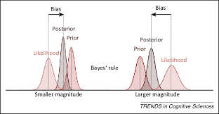
统计代写|贝叶斯分析代写Bayesian Analysis代考|BAYES’ RULE
Bayes’ rule is a basic result in probability that describes a relationship between two conditional distributions $p(X \mid Y)$ and $p(Y \mid X)$ for a pair of random variables (these random variables can also be continuous). More specifically, Bayes’ rule states that for any such pair of random variables, the following identity holds:
$$
p(Y=y \mid X=x)=\frac{p(X-x \mid Y-y) p(Y-y)}{p(X=x)}
$$
This result also generally holds true for any two events $A$ and $B$ with the conditional probability $p(X \in A \mid Y \in B)$.
The main advantage that Bayes’ rule offers is inversion of the conditional relationship between two random variables – therefore, if one variable is known, then the other can be calculated as well, assuming the marginal distributions $p(X=x)$ and $p(Y=y)$ are also known.
Bayes’ rule can be proven in several ways. One way to derive it is simply by using the chain rule twice. More specifically, we know that the joint distribution values can be rewritten as follows, using the chain rule, either first separating $X$ or first separating $Y$ :
$$
\begin{aligned}
p(X&=x, Y=y) \
&=p(X=x) p(Y=y \mid X=x) \
&=p(Y=y) p(X=x \mid Y=y)
\end{aligned}
$$
Taking the last equality above, $p(X=x) p(Y=y \mid X=x)=p(Y=y) p(X=x \mid Y=$ $y)$, and dividing both sides by $p(X=x)$ results in Bayes’ rule as described in Equation 1.2.
Bayes’ rule is the main pillar in Bayesian statistics for reasoning and learning from data. Bayes’ rule can invert the relationship between “observations” (the data) and the random variables we are interested in predicting. This makes it possible to infer target predictions from such observations. A more detailed description of these ideas is provided in Section 1.5, where statistical modeling is discussed.
贝叶斯分析代考
统计代写|贝叶斯分析代写Bayesian Analysis代考|JOINT DISTRIBUTION OVER MULTIPLE RANDOM VARIABLES
可以在同一个样本空间上定义多个随机变量。例如,对于一个离散的样本空间,比如一组词,我们可以定义两个随 机变量 $X$ 和 $Y$ 取整数值一一一个可以测量单词长度,另一个可以测量单词中元音的数量。给定两个这样的随机变 量,联合分布 $P(X, Y)$ 是映射成对事件的函数 $(A, B)$ 如下:
$$
p(X \in A, Y \in B)=p\left(X^{-1}(A) \cap Y^{-1}(B)\right)
$$
$\mathrm{~ 我 们 经 常 会 采 取 几 组 ~ V e f t { 1 O m e g a _ { 1 } , ~ \ d o t s , ~ I O m e g a _ { m }}$ $\Omega=\Omega_{1} \times \ldots \times \Omega_{m}$. 每个 $\Omega_{i}$ 与随机变量相关联。基于此,可以为所有这些随机变量一起定义联合概率分布。例 如,考虑 $\Omega=V \times P$ 在哪里 $V$ 是一个词汇表和 $P$ 是词性标签。这个样本空间使我们能够定义概率 $p(x, y)$ 在哪里 $X$ 表示与词性相关的词 $Y$. 在这种情况下, $x \in V$ 和 $y \in P$.
对于任何联合分布,我们可以边缘化一些随机变量以获得在原始随机变量的子集上定义的分布(因此它仍然可以是 联合分布,仅在随机变量的子集上)。使用积分 (对于连续变量) 或求和 (对于离散随机变量) 进行边缘化。这种 求和或积分操作从联合分布中消除了随机变量。结果是非边缘化随机变量的联合分布。
对于上面简单的词性示例,我们可以得到边缘 $p(x)=\sum_{y \in P} p(x, y)$ 或者 $p(y)=\sum_{x \in V} p(x, y)$. 边缘人 $p(X)$ 和 $p(Y)$ 不唯一确定联合分布值 $p(X, Y)$. 只有反过来才是正确的。然而,每当 $X$ 和 $Y$ 是独立的,则可以使用边际确 定联合分布。在第 $1.3 .2$ 节中了解更多信息。
统计代写|贝叶斯分析代写Bayesian Analysis代考|CONDITIONAL DISTRIBUTIONS
联合概率分布为有关几个随机变量获得特定值的概率问题提供了答案。条件分布为不同但相关的问题提供了答案。 当联合分布中的其他变量被限制为特定值时(或当它们被”钅制”时),它们有助于确定随机变量可以获得的值。
条件分布可从同一组随机变量上的联合分布推导出来。考虑一对随机变量 $X$ 和 $Y$ (连续的或离散的)。如果 $A$ 是来 自样本空间的事件 $X$ 和 $y$ 是样本空间中的一个值 $Y$ ,然后:
$$
p(X \in A \mid Y=y)=\frac{p(X \in A, Y=y)}{p(Y=y)}
$$
将被解释为确定概率的条件分布 $X \in A$ 以 $Y$ 获取价值 $y$. 条形表示我们正在夹紧 $Y$ 到价值 $y$ 并确定引起的分布 $X$ 在有 限的样本空间中。非正式地,条件分布占据样本空间的一部分,其中 $Y=y$ 并重新归一化联合分布,使得结果是仅 在样本空间的该部分上定义的概率分布。
当我们考虑方程中的联合分布时 $1.1$ 是一个将事件映射到空间中的概率的函数 $X$ ,和 $y$ 是固定的,我们注意到,价 值 $p(Y=y)$ 实际上是一个归一化常数,可以从分子中确定 $p(X \in A, Y=y)$. 例如,如果 $X$ 使用 PMF 时是离散 的,则:
$$
p(Y=y)=\sum_{x} p(X=x, Y=y)
$$
统计代写|贝叶斯分析代写Bayesian Analysis代考|BAYES’ RULE
贝叶斯规则是描述两个条件分布之间关系的概率的基本结果 $p(X \mid Y)$ 和 $p(Y \mid X)$ 对于一对随机变量 (这些随机 变量也可以是连续的)。更具体地说,贝叶斯规则指出,对于任何这样的随机变量对,以下恒等式成立:
$$
p(Y=y \mid X=x)=\frac{p(X-x \mid Y-y) p(Y-y)}{p(X=x)}
$$
这个结果通常也适用于任何两个事件 $A$ 和 $B$ 有条件概率 $p(X \in A \mid Y \in B)$.
贝叶斯规则提供的主要优点是反转两个随机变量之间的条件关系一一因此,如果一个变量是已知的,那么假设边际 分布也可以计算另一个变量 $p(X=x)$ 和 $p(Y=y)$ 也是众所周知的。
贝叶斯规则可以通过多种方式证明。推导它的一种方法是简单地使用链式法则两次。更具体地说,我们知道联合分 布值可以改写如下,使用链式法则,或者首先分离 $X$ 或先分离 $Y:$
$$
p(X=x, Y=y) \quad=p(X=x) p(Y=y \mid X=x)=p(Y=y) p(X=x \mid Y=y)
$$
取上面最后一个等式, $p(X=x) p(Y=y \mid X=x)=p(Y=y) p(X=x \mid Y=y)$ ,并将两边除以 $p(X=x)$ 得出公式 $1.2$ 中描述的贝叶斯规则。
贝叶斯规则是贝叶斯统计中用于推理和从数据中学习的主要支柱。贝叶斯规则可以颠倒“观察”(数据)和我们有兴 趣预测的随机变量之间的关系。这使得从这些观察中推断出目标预测成为可能。1.5节提供了对这些想法的更详细 描述,其中讨论了统计建模。

统计代写请认准statistics-lab™. statistics-lab™为您的留学生涯保驾护航。
金融工程代写
金融工程是使用数学技术来解决金融问题。金融工程使用计算机科学、统计学、经济学和应用数学领域的工具和知识来解决当前的金融问题,以及设计新的和创新的金融产品。
非参数统计代写
非参数统计指的是一种统计方法,其中不假设数据来自于由少数参数决定的规定模型;这种模型的例子包括正态分布模型和线性回归模型。
广义线性模型代考
广义线性模型(GLM)归属统计学领域,是一种应用灵活的线性回归模型。该模型允许因变量的偏差分布有除了正态分布之外的其它分布。
术语 广义线性模型(GLM)通常是指给定连续和/或分类预测因素的连续响应变量的常规线性回归模型。它包括多元线性回归,以及方差分析和方差分析(仅含固定效应)。
有限元方法代写
有限元方法(FEM)是一种流行的方法,用于数值解决工程和数学建模中出现的微分方程。典型的问题领域包括结构分析、传热、流体流动、质量运输和电磁势等传统领域。
有限元是一种通用的数值方法,用于解决两个或三个空间变量的偏微分方程(即一些边界值问题)。为了解决一个问题,有限元将一个大系统细分为更小、更简单的部分,称为有限元。这是通过在空间维度上的特定空间离散化来实现的,它是通过构建对象的网格来实现的:用于求解的数值域,它有有限数量的点。边界值问题的有限元方法表述最终导致一个代数方程组。该方法在域上对未知函数进行逼近。[1] 然后将模拟这些有限元的简单方程组合成一个更大的方程系统,以模拟整个问题。然后,有限元通过变化微积分使相关的误差函数最小化来逼近一个解决方案。
tatistics-lab作为专业的留学生服务机构,多年来已为美国、英国、加拿大、澳洲等留学热门地的学生提供专业的学术服务,包括但不限于Essay代写,Assignment代写,Dissertation代写,Report代写,小组作业代写,Proposal代写,Paper代写,Presentation代写,计算机作业代写,论文修改和润色,网课代做,exam代考等等。写作范围涵盖高中,本科,研究生等海外留学全阶段,辐射金融,经济学,会计学,审计学,管理学等全球99%专业科目。写作团队既有专业英语母语作者,也有海外名校硕博留学生,每位写作老师都拥有过硬的语言能力,专业的学科背景和学术写作经验。我们承诺100%原创,100%专业,100%准时,100%满意。
随机分析代写
随机微积分是数学的一个分支,对随机过程进行操作。它允许为随机过程的积分定义一个关于随机过程的一致的积分理论。这个领域是由日本数学家伊藤清在第二次世界大战期间创建并开始的。
时间序列分析代写
随机过程,是依赖于参数的一组随机变量的全体,参数通常是时间。 随机变量是随机现象的数量表现,其时间序列是一组按照时间发生先后顺序进行排列的数据点序列。通常一组时间序列的时间间隔为一恒定值(如1秒,5分钟,12小时,7天,1年),因此时间序列可以作为离散时间数据进行分析处理。研究时间序列数据的意义在于现实中,往往需要研究某个事物其随时间发展变化的规律。这就需要通过研究该事物过去发展的历史记录,以得到其自身发展的规律。
回归分析代写
多元回归分析渐进(Multiple Regression Analysis Asymptotics)属于计量经济学领域,主要是一种数学上的统计分析方法,可以分析复杂情况下各影响因素的数学关系,在自然科学、社会和经济学等多个领域内应用广泛。
MATLAB代写
MATLAB 是一种用于技术计算的高性能语言。它将计算、可视化和编程集成在一个易于使用的环境中,其中问题和解决方案以熟悉的数学符号表示。典型用途包括:数学和计算算法开发建模、仿真和原型制作数据分析、探索和可视化科学和工程图形应用程序开发,包括图形用户界面构建MATLAB 是一个交互式系统,其基本数据元素是一个不需要维度的数组。这使您可以解决许多技术计算问题,尤其是那些具有矩阵和向量公式的问题,而只需用 C 或 Fortran 等标量非交互式语言编写程序所需的时间的一小部分。MATLAB 名称代表矩阵实验室。MATLAB 最初的编写目的是提供对由 LINPACK 和 EISPACK 项目开发的矩阵软件的轻松访问,这两个项目共同代表了矩阵计算软件的最新技术。MATLAB 经过多年的发展,得到了许多用户的投入。在大学环境中,它是数学、工程和科学入门和高级课程的标准教学工具。在工业领域,MATLAB 是高效研究、开发和分析的首选工具。MATLAB 具有一系列称为工具箱的特定于应用程序的解决方案。对于大多数 MATLAB 用户来说非常重要,工具箱允许您学习和应用专业技术。工具箱是 MATLAB 函数(M 文件)的综合集合,可扩展 MATLAB 环境以解决特定类别的问题。可用工具箱的领域包括信号处理、控制系统、神经网络、模糊逻辑、小波、仿真等。