分类: 线性回归代写

统计代写|STAT311 Linear regression

Statistics-lab™可以为您提供metrostate.edu STAT311 Linear regression线性回归课程的代写代考辅导服务!

STAT311 Linear regression课程简介

This course covers various statistical models such as simple linear regression, multiple regression, and analysis of variance. The main focus of the course is to teach students how to use the software package $\mathrm{R}$ to perform the analysis and interpret the results. Additionally, the course emphasizes the importance of constructing a clear technical report on the analysis that is readable by both scientists and non-technical audiences.

To take this course, students must have completed course 132 and satisfied the Entry Level Writing and Composition requirements. This course satisfies the General Education Code W requirement.

PREREQUISITES 

Covers simple linear regression, multiple regression, and analysis of variance models. Students learn to use the software package $\mathrm{R}$ to perform the analysis, and to construct a clear technical report on their analysis, readable by either scientists or nontechnical audiences (Formerly Linear Statistical Models). Prerequisite(s): course 132 and satisfaction of the Entry Level Writing and Composition requirements. Gen. Ed. Code(s): W

STAT311 Linear regression HELP(EXAM HELP, ONLINE TUTOR)

问题 1.

Proposition 3.1. Suppose that a numerical variable selection method suggests several submodels with $k$ predictors, including a constant, where $2 \leq k \leq p$
a) The model $I$ that minimizes $C_p(I)$ maximizes $\operatorname{corr}\left(r, r_I\right)$.
b) $C_p(I) \leq 2 k$ implies that $\operatorname{corr}\left(\mathrm{r}, \mathrm{r}{\mathrm{I}}\right) \geq \sqrt{1-\frac{\mathrm{p}}{\mathrm{n}}}$. c) As $\operatorname{corr}\left(r, r_I\right) \rightarrow 1$, $$ \operatorname{corr}\left(\boldsymbol{x}^{\mathrm{T}} \hat{\boldsymbol{\beta}}, \boldsymbol{x}{\mathrm{I}}^{\mathrm{T}} \hat{\boldsymbol{\beta}}{\mathrm{I}}\right)=\operatorname{corr}(\mathrm{ESP}, \mathrm{ESP}(\mathrm{I}))=\operatorname{corr}\left(\hat{\mathrm{Y}}, \hat{\mathrm{Y}}{\mathrm{I}}\right) \rightarrow 1
$$

Remark 3.1. Consider the model $I_i$ that deletes the predictor $x_i$. Then the model has $k=p-1$ predictors including the constant, and the test statistic is $t_i$ where
$$
t_i^2=F_{I_i}
$$
Using Definition 3.8 and $C_p\left(I_{\text {full }}\right)=p$, it can be shown that
$$
C_p\left(I_i\right)=C_p\left(I_{\text {full }}\right)+\left(t_i^2-2\right) .
$$
Using the screen $C_p(I) \leq \min (2 k, p)$ suggests that the predictor $x_i$ should not be deleted if
$$
\left|t_i\right|>\sqrt{2} \approx 1.414
$$
If $\left|t_i\right|<\sqrt{2}$, then the predictor can probably be deleted since $C_p$ decreases. The literature suggests using the $C_p(I) \leq k$ screen, but this screen eliminates too many potentially useful submodels.

问题 2.

Proposition 3.2. Suppose that every submodel contains a constant and that $\boldsymbol{X}$ is a full rank matrix.
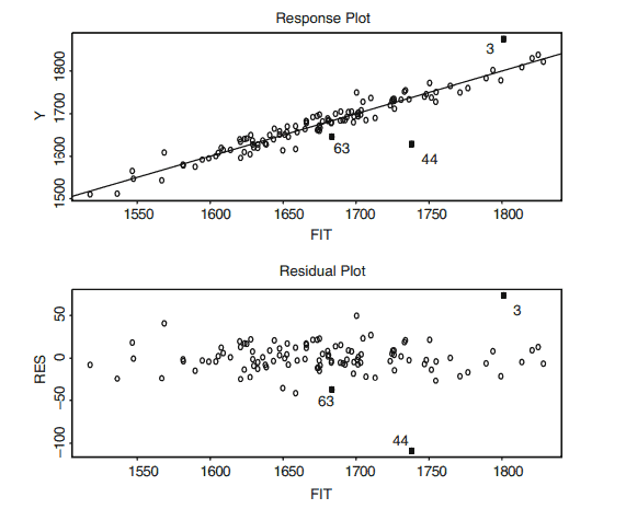
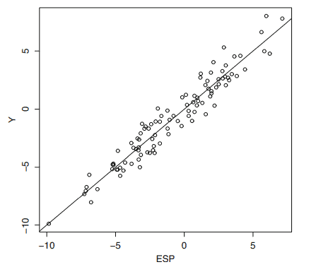
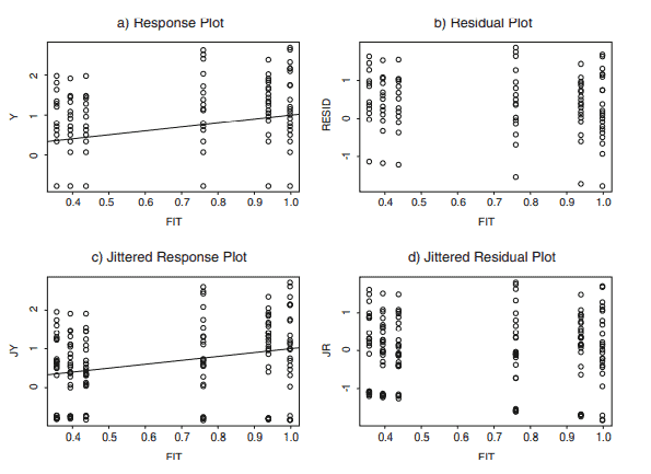
Response Plot: i) If $w=\hat{Y}I$ and $z=Y$, then the OLS line is the identity line. ii) If $w=Y$ and $z=\hat{Y}_I$, then the OLS line has slope $b=\left[\operatorname{corr}\left(Y, \hat{Y}_I\right)\right]^2=$ $R^2(I)$ and intercept $a=\bar{Y}\left(1-R^2(I)\right)$ where $\bar{Y}=\sum{i=1}^n Y_i / n$ and $R^2(I)$ is the coefficient of multiple determination from the candidate model.
FF or EE Plot: iii) If $w=\hat{Y}_I$ and $z=\hat{Y}$, then the OLS line is the identity line. Note that $E S P(I)=\hat{Y}_I$ and $E S P=\hat{Y}$.
iv) If $w=\hat{Y}$ and $z=\hat{Y}_I$, then the OLS line has slope $b=\left[\operatorname{corr}\left(\hat{Y}, \hat{Y}_I\right)\right]^2=$ $S S R(I) / S S R$ and intercept $a=\bar{Y}[1-(S S R(I) / S S R)]$ where SSR is the regression sum of squares.
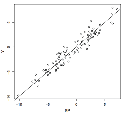
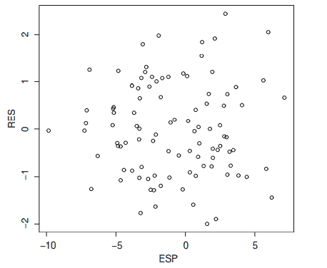
RR Plot: v) If $w=r$ and $z=r_I$, then the OLS line is the identity line.
vi) If $w=r_I$ and $z=r$, then $a=0$ and the OLS slope $b=\left[\operatorname{corr}\left(r, r_I\right)\right]^2$ and
$$
\operatorname{corr}\left(r, r_I\right)=\sqrt{\frac{S S E}{S S E(I)}}=\sqrt{\frac{n-p}{C_p(I)+n-2 k}}=\sqrt{\frac{n-p}{(p-k) F_I+n-p}} .
$$

Proof: Recall that $\boldsymbol{H}$ and $\boldsymbol{H}_I$ are symmetric idempotent matrices and that $\boldsymbol{H}_I=\boldsymbol{H}_I$. The mean of OLS fitted values is equal to $\bar{Y}$ and the mean of OLS residuals is equal to 0 . If the OLS line from regressing $z$ on $w$ is $\hat{z}=a+b w$, then $a=\bar{z}-b \bar{w}$ and $$
b=\frac{\sum\left(w_i-\bar{w}\right)\left(z_i-\bar{z}\right)}{\sum\left(w_i-\bar{w}\right)^2}=\frac{S D(z)}{S D(w)} \operatorname{corr}(z, w) .
$$
Also recall that the OLS line passes through the means of the two variables $(\bar{w}, \bar{z})$
$\left(^\right)$ Notice that the OLS slope from regressing $z$ on $w$ is equal to one if and only if the OLS slope from regressing $w$ on $z$ is equal to $[\operatorname{corr}(z, w)]^2$. i) The slope $b=1$ if $\sum \hat{Y}{I, i} Y_i=\sum \hat{Y}{I, i}^2$. This equality holds since $\hat{\boldsymbol{Y}}I^T \boldsymbol{Y}=$ $\boldsymbol{Y}^T \boldsymbol{H}_I \boldsymbol{Y}=\boldsymbol{Y}^T \boldsymbol{H}_I \boldsymbol{H}_I \boldsymbol{Y}=\hat{\boldsymbol{Y}}_I^T \hat{\boldsymbol{Y}}_I$. Since $b=1, a=\bar{Y}-\bar{Y}=0$. ii) By $\left(^\right)$, the slope
$$
b=\left[\operatorname{corr}\left(Y, \hat{Y}_I\right)\right]^2=R^2(I)=\frac{\sum\left(\hat{Y}{I, i}-\bar{Y}\right)^2}{\sum\left(Y_i-\bar{Y}\right)^2}=\operatorname{SSR}(I) / \operatorname{SSTO} .
$$
The result follows since $a=\bar{Y}-b \bar{Y}$.
iii) The slope $b=1$ if $\sum \hat{Y}{I, i} \hat{Y}_i=\sum \hat{Y}{I, i}^2$. This equality holds since $\hat{\boldsymbol{Y}}^T \hat{\boldsymbol{Y}}_I=\boldsymbol{Y}^T \boldsymbol{H} \boldsymbol{H}_I \boldsymbol{Y}=\boldsymbol{Y}^T \boldsymbol{H}_I \boldsymbol{Y}=\hat{\boldsymbol{Y}}_I^T \hat{\boldsymbol{Y}}_I$. Since $b=1, a=\bar{Y}-\bar{Y}=0$.
iv) From iii),
$$
1=\frac{S D(\hat{Y})}{S D\left(\hat{Y}_I\right)}\left[\operatorname{corr}\left(\hat{Y}, \hat{Y}_I\right)\right] .
$$

Textbooks


• An Introduction to Stochastic Modeling, Fourth Edition by Pinsky and Karlin (freely
available through the university library here)
• Essentials of Stochastic Processes, Third Edition by Durrett (freely available through
the university library here)
To reiterate, the textbooks are freely available through the university library. Note that
you must be connected to the university Wi-Fi or VPN to access the ebooks from the library
links. Furthermore, the library links take some time to populate, so do not be alarmed if
the webpage looks bare for a few seconds.

此图像的alt属性为空;文件名为%E7%B2%89%E7%AC%94%E5%AD%97%E6%B5%B7%E6%8A%A5-1024x575-10.png
统计代写|STAT311 Linear regression

Statistics-lab™可以为您提供metrostate.edu STAT311 Linear regression线性回归课程的代写代考辅导服务! 请认准Statistics-lab™. Statistics-lab™为您的留学生涯保驾护航。

统计代写|STAT311 Linear regression

Statistics-lab™可以为您提供metrostate.edu STAT311 Linear regression线性回归课程的代写代考辅导服务!

STAT311 Linear regression课程简介

This course covers various statistical models such as simple linear regression, multiple regression, and analysis of variance. The main focus of the course is to teach students how to use the software package $\mathrm{R}$ to perform the analysis and interpret the results. Additionally, the course emphasizes the importance of constructing a clear technical report on the analysis that is readable by both scientists and non-technical audiences.

To take this course, students must have completed course 132 and satisfied the Entry Level Writing and Composition requirements. This course satisfies the General Education Code W requirement.

PREREQUISITES 

Covers simple linear regression, multiple regression, and analysis of variance models. Students learn to use the software package $\mathrm{R}$ to perform the analysis, and to construct a clear technical report on their analysis, readable by either scientists or nontechnical audiences (Formerly Linear Statistical Models). Prerequisite(s): course 132 and satisfaction of the Entry Level Writing and Composition requirements. Gen. Ed. Code(s): W

STAT311 Linear regression HELP(EXAM HELP, ONLINE TUTOR)

问题 1.

2.10. In the above table, $x_i$ is the length of the femur and $y_i$ is the length of the humerus taken from five dinosaur fossils (Archaeopteryx) that preserved both bones. See Moore (2000, p. 99).
a) Complete the table and find the least squares estimators $\hat{\beta}_1$ and $\hat{\beta}_2$.
b) Predict the humerus length if the femur length is 60 .

问题 2.

2.11. Suppose that the regression model is $Y_i=7+\beta X_i+e_i$ for $i=$ $1, \ldots, n$ where the $e_i$ are iid $N\left(0, \sigma^2\right)$ random variables. The least squares criterion is $Q(\eta)=\sum_{i=1}^n\left(Y_i-7-\eta X_i\right)^2$.
a) What is $E\left(Y_i\right)$ ?
b) Find the least squares estimator $\beta$ of $\beta$ by setting the first derivative $\frac{d}{d \eta} Q(\eta)$ equal to zero.
c) Show that your $\hat{\beta}$ is the global minimizer of the least squares criterion $Q$ by showing that the second derivative $\frac{d^2}{d \eta^2} Q(\eta)>0$ for all values of $\eta$.

问题 3.

2.12. The location model is $Y_i=\mu+e_i$ for $i=1, \ldots, n$ where the $e_i$ are iid with mean $E\left(e_i\right)=0$ and constant variance $\operatorname{VAR}\left(e_i\right)=\sigma^2$. The least squares estimator $\hat{\mu}$ of $\mu$ minimizes the least squares criterion $Q(\eta)=\sum_{i=1}^n\left(Y_i-\eta\right)^2$. To find the least squares estimator, perform the following steps.

a) Find the derivative $\frac{a}{d \eta} Q$, set the derivative equal to zero and solve for
$\eta$. Call the solution $\hat{\mu}$.
b) To show that the solution was indeed the global minimizer of $Q$, show that $\frac{d^2}{d \eta^2} Q>0$ for all real $\eta$. (Then the solution $\hat{\mu}$ is a local min and $Q$ is convex, so $\hat{\mu}$ is the global min.)

问题 4.

2.14. Suppose that the regression model is $Y_i=10+2 X_{i 2}+\beta_3 X_{i 3}+e_i$ for $i=1, \ldots, n$ where the $e_i$ are iid $N\left(0, \sigma^2\right)$ random variables. The least squares criterion is $Q\left(\eta_3\right)=\sum_{i=1}^n\left(Y_i-10-2 X_{\mathrm{i} 2}-\eta_3 X_{i 3}\right)^2$. Find the least squares estimator $\hat{\beta}_3$ of $\beta_3$ by setting the first derivative $\frac{d}{d \eta_3} Q\left(\eta_3\right)$ equal to zero. Show that your $\hat{\beta}_3$ is the global minimizer of the least squares criterion $Q$ by showing that the second derivative $\frac{d^2}{d \eta_3^2} Q\left(\eta_3\right)>0$ for all values of $\eta_3$.

Textbooks


• An Introduction to Stochastic Modeling, Fourth Edition by Pinsky and Karlin (freely
available through the university library here)
• Essentials of Stochastic Processes, Third Edition by Durrett (freely available through
the university library here)
To reiterate, the textbooks are freely available through the university library. Note that
you must be connected to the university Wi-Fi or VPN to access the ebooks from the library
links. Furthermore, the library links take some time to populate, so do not be alarmed if
the webpage looks bare for a few seconds.

此图像的alt属性为空;文件名为%E7%B2%89%E7%AC%94%E5%AD%97%E6%B5%B7%E6%8A%A5-1024x575-10.png
统计代写|STAT311 Linear regression

Statistics-lab™可以为您提供metrostate.edu STAT311 Linear regression线性回归课程的代写代考辅导服务! 请认准Statistics-lab™. Statistics-lab™为您的留学生涯保驾护航。

统计代写|STAT311 Linear regression

Statistics-lab™可以为您提供metrostate.edu STAT311 Linear regression线性回归课程的代写代考辅导服务!

STAT311 Linear regression课程简介

This course covers various statistical models such as simple linear regression, multiple regression, and analysis of variance. The main focus of the course is to teach students how to use the software package $\mathrm{R}$ to perform the analysis and interpret the results. Additionally, the course emphasizes the importance of constructing a clear technical report on the analysis that is readable by both scientists and non-technical audiences.

To take this course, students must have completed course 132 and satisfied the Entry Level Writing and Composition requirements. This course satisfies the General Education Code W requirement.

PREREQUISITES 

Covers simple linear regression, multiple regression, and analysis of variance models. Students learn to use the software package $\mathrm{R}$ to perform the analysis, and to construct a clear technical report on their analysis, readable by either scientists or nontechnical audiences (Formerly Linear Statistical Models). Prerequisite(s): course 132 and satisfaction of the Entry Level Writing and Composition requirements. Gen. Ed. Code(s): W

STAT311 Linear regression HELP(EXAM HELP, ONLINE TUTOR)

问题 1.

11.1. Suppose $Y_i=\boldsymbol{x}_i^T \boldsymbol{\beta}+\epsilon_i$ where the errors are independent $N\left(0, \sigma^2\right)$. Then the likelihood function is
$$
L\left(\boldsymbol{\beta}, \sigma^2\right)=\left(2 \pi \sigma^2\right)^{-n / 2} \exp \left(\frac{-1}{2 \sigma^2}|\boldsymbol{y}-\boldsymbol{X} \boldsymbol{\beta}|^2\right) .
$$
a) Since the least squares estimator $\hat{\beta}$ minimizes $|\boldsymbol{y}-\boldsymbol{X} \boldsymbol{\beta}|^2$, show that $\hat{\boldsymbol{\beta}}$ is the MLE of $\boldsymbol{\beta}$.
b) Then find the MLE $\hat{\sigma}^2$ of $\sigma^2$.

问题 2.

11.3. Suppose $Y_i=\boldsymbol{x}i^T \boldsymbol{\beta}+\epsilon_i$ where the errors are independent $N\left(0, \sigma^2 / w_i\right)$ where $w_i>0$ are known constants. Then the likelihood function is $$ L\left(\boldsymbol{\beta}, \sigma^2\right)=\left(\prod{i=1}^n \sqrt{w_i}\right)\left(\frac{1}{\sqrt{2 \pi}}\right)^n \frac{1}{\sigma^n} \exp \left(\frac{-1}{2 \sigma^2} \sum_{i=1}^n w_i\left(y_i-\boldsymbol{x}_i^T \boldsymbol{\beta}\right)^2\right) .
$$ a) Suppose that $\hat{\boldsymbol{\beta}}W$ minimizes $\sum{i=1}^n w_i\left(y_i-\boldsymbol{x}_i^T \boldsymbol{\beta}\right)^2$. Show that $\hat{\boldsymbol{\beta}}_W$ is the MLE of $\boldsymbol{\beta}$.
b) Then find the MLE $\hat{\sigma}^2$ of $\sigma^2$.

问题 3.

11.2. Suppose $Y_i=\boldsymbol{x}i^T \boldsymbol{\beta}+e_i$ where the errors are iid double exponential $(0, \sigma)$ where $\sigma>0$. Then the likelihood function is $$ L(\boldsymbol{\beta}, \sigma)=\frac{1}{2^n} \frac{1}{\sigma^n} \exp \left(\frac{-1}{\sigma} \sum{i=1}^n\left|Y_i-\boldsymbol{x}i^T \boldsymbol{\beta}\right|\right) . $$ Suppose that $\tilde{\boldsymbol{\beta}}$ is a minimizer of $\sum{i=1}^n\left|Y_i-\boldsymbol{x}i^T \boldsymbol{\beta}\right|$. a) By direct maximization, show that $\tilde{\boldsymbol{\beta}}$ is an MLE of $\boldsymbol{\beta}$ regardless of the value of $\sigma$. b) Find an MLE of $\sigma$ by maximizing $$ L(\sigma) \equiv L(\tilde{\boldsymbol{\beta}}, \sigma)=\frac{1}{2^n} \frac{1}{\sigma^n} \exp \left(\frac{-1}{\sigma} \sum{i=1}^n\left|Y_i-\boldsymbol{x}_i^T \tilde{\boldsymbol{\beta}}\right|\right) .
$$

问题 4.

11.8. Let $Y \sim N\left(\mu, \sigma^2\right)$ so that $E(Y)=\mu$ and $\operatorname{Var}(Y)=\sigma^2=E\left(Y^2\right)-$ $[E(Y)]^2$. If $k \geq 2$ is an integer, then
$$
E\left(Y^k\right)=(k-1) \sigma^2 E\left(Y^{k-2}\right)+\mu E\left(Y^{k-1}\right) .
$$
Let $Z=(Y-\mu) / \sigma \sim N(0,1)$. Hence $\mu_k=E(Y-\mu)^k=\sigma^k E\left(Z^k\right)$. Use this fact and the above recursion relationship $E\left(Z^k\right)=(k-1) E\left(Z^{k-2}\right)$ to find a) $\mu_3$ and b) $\mu_4$.

Textbooks


• An Introduction to Stochastic Modeling, Fourth Edition by Pinsky and Karlin (freely
available through the university library here)
• Essentials of Stochastic Processes, Third Edition by Durrett (freely available through
the university library here)
To reiterate, the textbooks are freely available through the university library. Note that
you must be connected to the university Wi-Fi or VPN to access the ebooks from the library
links. Furthermore, the library links take some time to populate, so do not be alarmed if
the webpage looks bare for a few seconds.

此图像的alt属性为空;文件名为%E7%B2%89%E7%AC%94%E5%AD%97%E6%B5%B7%E6%8A%A5-1024x575-10.png
统计代写|STAT311 Linear regression

Statistics-lab™可以为您提供metrostate.edu STAT311 Linear regression线性回归课程的代写代考辅导服务! 请认准Statistics-lab™. Statistics-lab™为您的留学生涯保驾护航。

统计代写|STAT501 Linear regression

Statistics-lab™可以为您提供psu.edu STAT501 Linear regression线性回归课程的代写代考辅导服务!

STAT501 Linear regression课程简介

This course covers various statistical models such as simple linear regression, multiple regression, and analysis of variance. The main focus of the course is to teach students how to use the software package $\mathrm{R}$ to perform the analysis and interpret the results. Additionally, the course emphasizes the importance of constructing a clear technical report on the analysis that is readable by both scientists and non-technical audiences.

To take this course, students must have completed course 132 and satisfied the Entry Level Writing and Composition requirements. This course satisfies the General Education Code W requirement.

PREREQUISITES 

Covers simple linear regression, multiple regression, and analysis of variance models. Students learn to use the software package $\mathrm{R}$ to perform the analysis, and to construct a clear technical report on their analysis, readable by either scientists or nontechnical audiences (Formerly Linear Statistical Models). Prerequisite(s): course 132 and satisfaction of the Entry Level Writing and Composition requirements. Gen. Ed. Code(s): W

STAT501 Linear regression HELP(EXAM HELP, ONLINE TUTOR)

问题 1.

(4) Table 5 contains data for the number of dairy cows (thousands) in the U.S. in various years.

  • Enter the data into a spreadsheet so that $x$ represents the number of years since 1940. e.g enter $x=10$ for 1950 , enter $x=20$ for 1960 , etc.
  • Create the scatter plot for the number of cows $y$ (thousands) as a function of $x$ (years since 1940).
  • Adjust the minimum and maximum of the axes of each plot to slightly below and slightly above the data values.
  • Compute the regression equation using logarithmic regression. The trendline will be $y=a \ln (x)+b$ for some values of $a$ and $b$. Round $a$ and $b$ to the nearest whole number.
  • Use your regression equation to estimate the number of dairy cows in 2020 $(x=2020-1940=80)$.

YearNumber of Dairy Cows (thousands)
194023900
195023600
196016500
197012700
198012200
199010300
20009800
20109200
20209420

To create a scatter plot in a spreadsheet:

  1. Enter the data into two columns, with the year values in one column (let’s say column A) and the number of dairy cows values in another column (let’s say column B).
  2. Select both columns of data.
  3. Click on the “Insert” tab and then on the “Scatter” chart icon.
  4. Choose a scatter plot with markers only.

After creating the scatter plot, adjust the minimum and maximum of the axes by right-clicking on each axis and choosing “Format Axis.” In the “Format Axis” panel, choose “Fixed” for the minimum and maximum values and adjust them to slightly below and slightly above the data values.

Using logarithmic regression, we can find the equation of the line of best fit for this data. In Excel, we can add a trendline to the scatter plot by right-clicking on one of the data points and selecting “Add Trendline.” In the “Add Trendline” panel, select “Logarithmic” as the Trend/Regression type. This will add a trendline to the scatter plot with an equation in the form of $y = a\ln(x) + b$, where $a$ and $b$ are the coefficients of the regression equation.

The regression equation for this data is $y = -327\ln(x) + 10629$. Rounding $a$ and $b$ to the nearest whole number, we get $a=-327$ and $b=10629$.

To estimate the number of dairy cows in 2020, we substitute $x=80$ into the equation and get $y = -327\ln(80) + 10629 \approx 9317$. Therefore, the estimated number of dairy cows in 2020 is about 9317 thousand (or 9.317 million) cows.

问题 2.

Know how to tell whether the experiment is a fixed or random effects one way Anova. (Were the levels fixed or a random sample from a population of levels?)

In a one-way ANOVA, we are comparing the means of multiple groups or levels on a single variable or outcome. The distinction between a fixed effects and random effects one-way ANOVA depends on whether the levels being compared are considered fixed or random.

Fixed effects one-way ANOVA: The levels being compared are considered fixed, meaning that they are chosen in advance and are of specific interest to the researcher. The goal of the analysis is to make inferences about the specific levels that were included in the study. For example, if we want to compare the performance of students in three different schools, and those three schools were chosen specifically for the study, we would use a fixed effects one-way ANOVA.

Random effects one-way ANOVA: The levels being compared are considered a random sample from a larger population of possible levels. The goal of the analysis is to make inferences about the population of levels from which the sample was drawn. For example, if we want to compare the effectiveness of three different brands of fertilizer on plant growth, and those three brands were chosen at random from a larger population of possible brands, we would use a random effects one-way ANOVA.

To determine whether a one-way ANOVA is a fixed or random effects design, we need to know how the levels were selected for the study. If the levels were chosen in advance and are of specific interest to the researcher, it is a fixed effects design. If the levels are a random sample from a larger population, it is a random effects design.

Textbooks


• An Introduction to Stochastic Modeling, Fourth Edition by Pinsky and Karlin (freely
available through the university library here)
• Essentials of Stochastic Processes, Third Edition by Durrett (freely available through
the university library here)
To reiterate, the textbooks are freely available through the university library. Note that
you must be connected to the university Wi-Fi or VPN to access the ebooks from the library
links. Furthermore, the library links take some time to populate, so do not be alarmed if
the webpage looks bare for a few seconds.

此图像的alt属性为空;文件名为%E7%B2%89%E7%AC%94%E5%AD%97%E6%B5%B7%E6%8A%A5-1024x575-10.png
统计代写|STAT501 Linear regression

Statistics-lab™可以为您提供psu.edu STAT501 Linear regression线性回归课程的代写代考辅导服务! 请认准Statistics-lab™. Statistics-lab™为您的留学生涯保驾护航。

统计代写|线性回归代写linear regression代考|MATH5386

如果你也在 怎样代写线性回归linear regression这个学科遇到相关的难题,请随时右上角联系我们的24/7代写客服。

线性回归是对标量响应和一个或多个解释变量(也称为因变量和自变量)之间的关系进行建模的一种线性方法。一个解释变量的情况被称为简单线性回归。

statistics-lab™ 为您的留学生涯保驾护航 在代写线性回归linear regression方面已经树立了自己的口碑, 保证靠谱, 高质且原创的统计Statistics代写服务。我们的专家在代写线性回归linear regression代写方面经验极为丰富,各种代写线性回归linear regression相关的作业也就用不着说。

我们提供的线性回归linear regression及其相关学科的代写,服务范围广, 其中包括但不限于:

  • Statistical Inference 统计推断
  • Statistical Computing 统计计算
  • Advanced Probability Theory 高等概率论
  • Advanced Mathematical Statistics 高等数理统计学
  • (Generalized) Linear Models 广义线性模型
  • Statistical Machine Learning 统计机器学习
  • Longitudinal Data Analysis 纵向数据分析
  • Foundations of Data Science 数据科学基础
统计代写|线性回归代写linear regression代考|MATH5386

统计代写|线性回归代写linear regression代考|Checking Goodness of Fit

It is crucial to realize that an MLR model is not necessarily a useful model for the data, even if the data set consists of a response variable and several predictor variables. For example, a nonlinear regression model or a much more complicated model may be needed. Chapters 1 and 13 describe several alternative models. Let $p$ be the number of predictors and $n$ the number of cases. Assume that $n \geq 5 p$, then plots can be used to check whether the MLR model is useful for studying the data. This technique is known as checking the goodness of fit of the MLR model.

Notation. Plots will be used to simplify regression analysis, and in this text a plot of $W$ versus $Z$ uses $W$ on the horizontal axis and $Z$ on the vertical axis.

Definition 2.10. A scatterplot of $X$ versus $Y$ is a plot of $X$ versus $Y$ and is used to visualize the conditional distribution $Y \mid X$ of $Y$ given $X$.

Definition 2.11. A response plot is a plot of a variable $w_i$ versus $Y_i$. Typically $w_i$ is a linear combination of the predictors: $w_i=\boldsymbol{x}_i^T \boldsymbol{\eta}$ where $\boldsymbol{\eta}$ is a known $p \times 1$ vector. The most commonly used response plot is a plot of the fitted values $\widehat{Y}_i$ versus the response $Y_i$.

Proposition 2.1. Suppose that the regression estimator $\boldsymbol{b}$ of $\boldsymbol{\beta}$ is used to find the residuals $r_i \equiv r_i(\boldsymbol{b})$ and the fitted values $\widehat{Y}_i \equiv \widehat{Y}_i(\boldsymbol{b})=\boldsymbol{x}_i^T \boldsymbol{b}$. Then in the response plot of $\widehat{Y}_i$ versus $Y_i$, the vertical deviations from the identity line (that has unit slope and zero intercept) are the residuals $r_i(b)$.

Proof. The identity line in the response plot is $Y=\boldsymbol{x}^T \boldsymbol{b}$. Hence the vertical deviation is $Y_i-\boldsymbol{x}_i^T \boldsymbol{b}=r_i(\boldsymbol{b})$.

Definition 2.12. A residual plot is a plot of a variable $w_i$ versus the residuals $r_i$. The most commonly used residual plot is a plot of $\hat{Y}_i$ versus $r_i$.
Notation: For MLR, “the residual plot” will often mean the residual plot of $\hat{Y}_i$ versus $r_i$, and “the response plot” will often mean the plot of $\hat{Y}_i$ versus $Y_i^*$

If the unimodal MLR model as estimated by least squares is useful, then in the response plot the plotted points should scatter about the identity line while in the residual plot of $\hat{Y}$ versus $r$ the plotted points should scatter about the $r=0$ line (the horizontal axis) with no other pattern. Figures $1.2$ and $1.3$ show what a response plot and residual plot look like for an artificial MLR data set where the MLR regression relationship is rather strong in that the sample correlation $\operatorname{corr}(\tilde{Y}, Y)$ is near 1 . Figure $1.4$ shows a response plot where the response $Y$ is independent of the nontrivial predictors in the model. Here $\operatorname{corr}(\hat{Y}, Y)$ is near 0 but the points still scatter about the identity line. When the MLR relationship is very weak, the response plot will look like the residual plot.

统计代写|线性回归代写linear regression代考|Checking Lack of Fit

The response plot may look good while the residual plot suggests that the unimodal MLR model can be improved. Examining plots to find model violations is called checking for lack of fit. Again assume that $n \geq 5 p$.

The unimodal MLR model often provides a useful model for the data, but the following assumptions do need to be checked.
i) Is the MLR model appropriate?
ii) Are outliers present?
iii) Is the error variance constant or nonconstant? The constant variance assumption $\operatorname{VAR}\left(e_i\right) \equiv \sigma^2$ is known as homoscedasticity. The nonconstant variance assumption $\operatorname{VAR}\left(e_i\right)=\sigma_i^2$ is known as heteroscedasticity.
iv) Are any important predictors left out of the model?
v) Are the errors $e_1, \ldots, e_n$ iid?
vi) Are the errors $e_i$ independent of the predictors $\boldsymbol{x}_i$ ?
Make the response plot and the residual plot to check i), ii), and iii). An MLR model is reasonable if the plots look like Figures 1.2, 1.3, 1.4, and 2.1. A response plot that looks like Figure $13.7$ suggests that the model is not linear. If the plotted points in the residual plot do not scatter about the $r=0$ line with no other pattern (i.e., if the cloud of points is not ellipsoidal or rectangular with zero slope), then the unimodal MLR model is not sustained.
The $i$ th residual $r_i$ is an estimator of the $i$ th error $e_i$. The constant variance assumption may have been violated if the variability of the point cloud in the residual plot depends on the value of $\hat{Y}$. Often the variability of the residuals increases as $\hat{Y}$ increases, resulting in a right opening megaphone shape. (Figure $4.1 \mathrm{~b}$ has this shape.) Often the variability of the residuals decreases as $\hat{Y}$ increases, resulting in a left opening megaphone shape. Sometimes the variability decreases then increases again, and sometimes the variability increases then decreases again (like a stretched or compressed football).

统计代写|线性回归代写linear regression代考|MATH5386

线性回归代写

统计代写|线性回归代写线性回归代考|检验拟合优度


重要的是要认识到MLR模型不一定是数据的有用模型,即使数据集由一个响应变量和几个预测变量组成。例如,可能需要一个非线性回归模型或一个更复杂的模型。第1章和第13章描述了几种替代模型。设$p$为预测数,$n$为病例数。假设$n \geq 5 p$,那么可以使用图来检查MLR模型对研究数据是否有用。这种技术被称为检查MLR模型的拟合优度

符号。图将用于简化回归分析,在本文中$W$与$Z$的图使用$W$作为横轴,$Z$作为纵轴。

定义$X$ vs . $Y$的散点图是$X$ vs . $Y$的散点图,用于可视化给定$X$时$Y$的条件分布$Y \mid X$

定义响应图是一个变量$w_i$和$Y_i$的图。通常$w_i$是预测器的线性组合:$w_i=\boldsymbol{x}_i^T \boldsymbol{\eta}$,其中$\boldsymbol{\eta}$是已知的$p \times 1$向量。最常用的响应曲线是拟合值$\widehat{Y}_i$与响应$Y_i$的曲线。

假设用$\boldsymbol{\beta}$的回归估计量$\boldsymbol{b}$求残差$r_i \equiv r_i(\boldsymbol{b})$和拟合值$\widehat{Y}_i \equiv \widehat{Y}_i(\boldsymbol{b})=\boldsymbol{x}_i^T \boldsymbol{b}$。然后在$\widehat{Y}_i$对$Y_i$的响应图中,与恒等线(具有单位斜率和零截距)的垂直偏差为残差$r_i(b)$ .

证明。响应图中的标识线是$Y=\boldsymbol{x}^T \boldsymbol{b}$。因此垂直偏差为$Y_i-\boldsymbol{x}_i^T \boldsymbol{b}=r_i(\boldsymbol{b})$ .

定义残差图是一个变量$w_i$和残差$r_i$的图。最常用的残差图是$\hat{Y}_i$对$r_i$的残差图
符号:对于MLR,“残差图”通常表示$\hat{Y}_i$对$r_i$的残差图,“响应图”通常表示$\hat{Y}_i$对$Y_i^*$的残差图


如果由最小二乘估计的单峰MLR模型是有用的,那么在响应图中,绘制的点应该分散在标识线附近,而在$\hat{Y}$对$r$的残差图中,绘制的点应该分散在$r=0$线(水平轴)附近,没有其他模式。图$1.2$和$1.3$显示了人工MLR数据集的响应图和残差图,其中MLR回归关系相当强,因为样本相关性$\operatorname{corr}(\tilde{Y}, Y)$接近1。图$1.4$显示了响应图,其中响应$Y$独立于模型中的非平凡预测器。这里$\operatorname{corr}(\hat{Y}, Y)$接近0,但点仍然分散在恒等线上。当MLR关系很弱时,响应图看起来像残差图

统计代写|线性回归代写线性回归代考|检查不符合

. . . .

响应图可能看起来不错,而残差图表明单峰MLR模型可以改进。检查图以发现模型违反称为检查缺乏拟合。再次假设$n \geq 5 p$ .


单峰MLR模型通常为数据提供了一个有用的模型,但需要检查以下假设:
i) MLR模型是否合适?
ii)是否存在异常值?
iii)误差方差是常数还是非常数?恒定方差假设 $\operatorname{VAR}\left(e_i\right) \equiv \sigma^2$ 被称为同异性。非常数方差假设 $\operatorname{VAR}\left(e_i\right)=\sigma_i^2$
iv)模型中是否遗漏了任何重要的预测因子?
v)是否存在误差 $e_1, \ldots, e_n$
vi)错误 $e_i$ 独立于预测因子 $\boldsymbol{x}_i$ ?
绘制响应图和残差图,以检验i), ii)和iii)。如果图如图1.2,1.3,1.4和2.1所示,则MLR模型是合理的。响应图如图所示 $13.7$ 说明模型不是线性的。如果残差图中的点不分散在 $r=0$ 没有其他模式(即,如果点云不是椭球形或斜率为零的矩形),则单峰MLR模型不成立。
$i$ 残差 $r_i$ 的估计值 $i$ 错误 $e_i$。如果残差图中点云的可变性取决于的值,则可能违反恒定方差假设 $\hat{Y}$。通常残差的可变性会随着 $\hat{Y}$ 增加,导致右开口扩音器形状。(图 $4.1 \mathrm{~b}$ 有这个形状。)残差的变异性往往随着 $\hat{Y}$ 增加,导致左侧开口扩音器形状。有时可变性会减小然后再次增大,有时可变性会增大然后再次减小(就像一个拉伸或压缩的足球)

统计代写|线性回归代写linear regression代考 请认准statistics-lab™

统计代写请认准statistics-lab™. statistics-lab™为您的留学生涯保驾护航。

金融工程代写

金融工程是使用数学技术来解决金融问题。金融工程使用计算机科学、统计学、经济学和应用数学领域的工具和知识来解决当前的金融问题,以及设计新的和创新的金融产品。

非参数统计代写

非参数统计指的是一种统计方法,其中不假设数据来自于由少数参数决定的规定模型;这种模型的例子包括正态分布模型和线性回归模型。

广义线性模型代考

广义线性模型(GLM)归属统计学领域,是一种应用灵活的线性回归模型。该模型允许因变量的偏差分布有除了正态分布之外的其它分布。

术语 广义线性模型(GLM)通常是指给定连续和/或分类预测因素的连续响应变量的常规线性回归模型。它包括多元线性回归,以及方差分析和方差分析(仅含固定效应)。

有限元方法代写

有限元方法(FEM)是一种流行的方法,用于数值解决工程和数学建模中出现的微分方程。典型的问题领域包括结构分析、传热、流体流动、质量运输和电磁势等传统领域。

有限元是一种通用的数值方法,用于解决两个或三个空间变量的偏微分方程(即一些边界值问题)。为了解决一个问题,有限元将一个大系统细分为更小、更简单的部分,称为有限元。这是通过在空间维度上的特定空间离散化来实现的,它是通过构建对象的网格来实现的:用于求解的数值域,它有有限数量的点。边界值问题的有限元方法表述最终导致一个代数方程组。该方法在域上对未知函数进行逼近。[1] 然后将模拟这些有限元的简单方程组合成一个更大的方程系统,以模拟整个问题。然后,有限元通过变化微积分使相关的误差函数最小化来逼近一个解决方案。

tatistics-lab作为专业的留学生服务机构,多年来已为美国、英国、加拿大、澳洲等留学热门地的学生提供专业的学术服务,包括但不限于Essay代写,Assignment代写,Dissertation代写,Report代写,小组作业代写,Proposal代写,Paper代写,Presentation代写,计算机作业代写,论文修改和润色,网课代做,exam代考等等。写作范围涵盖高中,本科,研究生等海外留学全阶段,辐射金融,经济学,会计学,审计学,管理学等全球99%专业科目。写作团队既有专业英语母语作者,也有海外名校硕博留学生,每位写作老师都拥有过硬的语言能力,专业的学科背景和学术写作经验。我们承诺100%原创,100%专业,100%准时,100%满意。

随机分析代写


随机微积分是数学的一个分支,对随机过程进行操作。它允许为随机过程的积分定义一个关于随机过程的一致的积分理论。这个领域是由日本数学家伊藤清在第二次世界大战期间创建并开始的。

时间序列分析代写

随机过程,是依赖于参数的一组随机变量的全体,参数通常是时间。 随机变量是随机现象的数量表现,其时间序列是一组按照时间发生先后顺序进行排列的数据点序列。通常一组时间序列的时间间隔为一恒定值(如1秒,5分钟,12小时,7天,1年),因此时间序列可以作为离散时间数据进行分析处理。研究时间序列数据的意义在于现实中,往往需要研究某个事物其随时间发展变化的规律。这就需要通过研究该事物过去发展的历史记录,以得到其自身发展的规律。

回归分析代写

多元回归分析渐进(Multiple Regression Analysis Asymptotics)属于计量经济学领域,主要是一种数学上的统计分析方法,可以分析复杂情况下各影响因素的数学关系,在自然科学、社会和经济学等多个领域内应用广泛。

MATLAB代写

MATLAB 是一种用于技术计算的高性能语言。它将计算、可视化和编程集成在一个易于使用的环境中,其中问题和解决方案以熟悉的数学符号表示。典型用途包括:数学和计算算法开发建模、仿真和原型制作数据分析、探索和可视化科学和工程图形应用程序开发,包括图形用户界面构建MATLAB 是一个交互式系统,其基本数据元素是一个不需要维度的数组。这使您可以解决许多技术计算问题,尤其是那些具有矩阵和向量公式的问题,而只需用 C 或 Fortran 等标量非交互式语言编写程序所需的时间的一小部分。MATLAB 名称代表矩阵实验室。MATLAB 最初的编写目的是提供对由 LINPACK 和 EISPACK 项目开发的矩阵软件的轻松访问,这两个项目共同代表了矩阵计算软件的最新技术。MATLAB 经过多年的发展,得到了许多用户的投入。在大学环境中,它是数学、工程和科学入门和高级课程的标准教学工具。在工业领域,MATLAB 是高效研究、开发和分析的首选工具。MATLAB 具有一系列称为工具箱的特定于应用程序的解决方案。对于大多数 MATLAB 用户来说非常重要,工具箱允许您学习应用专业技术。工具箱是 MATLAB 函数(M 文件)的综合集合,可扩展 MATLAB 环境以解决特定类别的问题。可用工具箱的领域包括信号处理、控制系统、神经网络、模糊逻辑、小波、仿真等。

R语言代写问卷设计与分析代写
PYTHON代写回归分析与线性模型代写
MATLAB代写方差分析与试验设计代写
STATA代写机器学习/统计学习代写
SPSS代写计量经济学代写
EVIEWS代写时间序列分析代写
EXCEL代写深度学习代写
SQL代写各种数据建模与可视化代写

统计代写|线性回归代写linear regression代考|MATH839

如果你也在 怎样代写线性回归linear regression这个学科遇到相关的难题,请随时右上角联系我们的24/7代写客服。

线性回归是对标量响应和一个或多个解释变量(也称为因变量和自变量)之间的关系进行建模的一种线性方法。一个解释变量的情况被称为简单线性回归。

statistics-lab™ 为您的留学生涯保驾护航 在代写线性回归linear regression方面已经树立了自己的口碑, 保证靠谱, 高质且原创的统计Statistics代写服务。我们的专家在代写线性回归linear regression代写方面经验极为丰富,各种代写线性回归linear regression相关的作业也就用不着说。

我们提供的线性回归linear regression及其相关学科的代写,服务范围广, 其中包括但不限于:

  • Statistical Inference 统计推断
  • Statistical Computing 统计计算
  • Advanced Probability Theory 高等概率论
  • Advanced Mathematical Statistics 高等数理统计学
  • (Generalized) Linear Models 广义线性模型
  • Statistical Machine Learning 统计机器学习
  • Longitudinal Data Analysis 纵向数据分析
  • Foundations of Data Science 数据科学基础
统计代写|线性回归代写linear regression代考|MATH839

统计代写|线性回归代写linear regression代考|Variable Selection

A standard problem in $1 \mathrm{D}$ regression is variable selection, also called subset or model selection. Assume that the 1D regression model uses a linear predictor
$$
Y \Perp \boldsymbol{x} \mid\left(\alpha+\boldsymbol{\beta}^T \boldsymbol{x}\right),
$$
that a constant $\alpha$ is always included, that $\boldsymbol{x}=\left(x_1, \ldots, x_{p-1}\right)^T$ are the $p-1$ nontrivial predictors, and that the $n \times p$ matrix $\boldsymbol{X}$ with $i$ th row $\left(1, \boldsymbol{x}_i^T\right)$ has full rank $p$. Then variable selection is a search for a subset of predictor variables that can be deleted without important loss of information.

To clarify ideas, assume that there exists a subset $S$ of predictor variables such that if $x_S$ is in the $1 \mathrm{D}$ model, then none of the other predictors are needed in the model. Write $E$ for these (‘extraneous’) variables not in $S$, partitioning $\boldsymbol{x}=\left(\boldsymbol{x}_S^T, \boldsymbol{x}_E^T\right)^T$. Then
$$
S P=\alpha+\boldsymbol{\beta}^T \boldsymbol{x}=\alpha+\boldsymbol{\beta}_S^T \boldsymbol{x}_S+\boldsymbol{\beta}_E^T \boldsymbol{x}_E=\alpha+\boldsymbol{\beta}_S^T \boldsymbol{x}_S .
$$
The extraneous terms that can be eliminated given that the subset $S$ is in the model have zero coefficients: $\boldsymbol{\beta}_E=\mathbf{0}$.

Now suppose that $I$ is a candidate subset of predictors, that $S \subseteq I$ and that $O$ is the set of predictors not in $I$. Then
$$
S P-\alpha+\boldsymbol{\beta}^T \boldsymbol{x}-\alpha+\boldsymbol{\beta}S^T \boldsymbol{x}_S-\alpha+\boldsymbol{\beta}_S^T \boldsymbol{x}_S+\boldsymbol{\beta}{(I / S)}^T \boldsymbol{x}{I / S}+\mathbf{0}^T \boldsymbol{x}_O-\alpha+\boldsymbol{\beta}_I^T \boldsymbol{x}_I, $$ where $\boldsymbol{x}{I / S}$ denotes the predictors in $I$ that are not in $S$. Since this is true regardless of the values of the predictors, $\boldsymbol{\beta}O=\mathbf{0}$ if $S \subseteq I$. Hence for any subset $I$ that includes all relevant predictors, the population correlation $$ \operatorname{corr}\left(\alpha+\boldsymbol{\beta}^{\mathrm{T}} \boldsymbol{x}{\mathrm{i}}, \alpha+\boldsymbol{\beta}{\mathrm{I}}^{\mathrm{T}} \boldsymbol{x}{\mathrm{I}, \mathrm{i}}\right)=1 .
$$
This observation, which is true regardless of the explanatory power of the model, suggests that variable selection for a $1 \mathrm{D}$ regression model (1.11) is simple in principle. For each value of $j=1,2, \ldots, p-1$ nontrivial predictors, keep track of subsets $I$ that provide the largest values of corr(ESP,ESP $(I))$. Any such subset for which the correlation is high is worth closer investigation and consideration.

统计代写|线性回归代写linear regression代考|Other Issues

The $1 \mathrm{D}$ regression models offer a unifying framework for many of the most used regression models. By writing the model in terms of the sufficient predictor $S P=h(\boldsymbol{x})$, many important topics valid for all $1 \mathrm{D}$ regression models can be explained compactly. For example, the previous section presented variable selection, and equation (1.14) can be used to motivate the test for whether the reduced model can be used instead of the full model. Similarly, the sufficient predictor can be used to unify the interpretation of coefficients and to explain models that contain interactions and factors.
Interpretation of Coefficients
One interpretation of the coefficients in a 1D model (1.11) is that $\beta_i$ is the rate of change in the SP associated with a unit increase in $x_i$ when all other predictor variables $x_1, \ldots, x_{i-1}, x_{i+1}, \ldots, x_p$ are held fixed. Denote a model by $S P=\alpha+\boldsymbol{\beta}^T \boldsymbol{x}=\alpha+\beta_1 x_1+\cdots+\beta_p x_p$. Then
$$
\beta_i=\frac{\partial S P}{\partial x_i} \text { for } \mathrm{i}=1, \ldots, \mathrm{p} .
$$
Of course, holding all other variables fixed while changing $x_i$ may not be possible. For example, if $x_1=x, x_2=x^2$ and $S P=\alpha+\beta_1 x+\beta_2 x^2$, then $x_2$ cannot be held fixed when $x_1$ increases by one unit, but
$$
\frac{d S P}{d x}=\beta_1+2 \beta_2 x .
$$
The interpretation of $\beta_i$ changes with the model in two ways. First, the interpretation changes as terms are added and deleted from the SP. Hence the interpretation of $\beta_1$ differs for models $S P=\alpha+\beta_1 x_1$ and $S P=\alpha+\beta_1 x_1+\beta_2 x_2$. Secondly, the interpretation changes as the parametric or semiparametric form of the model changes.

统计代写|线性回归代写linear regression代考|MATH839

线性回归代写

统计代写|线性回归代写线性回归代考|变量选择


$1 \mathrm{D}$回归中的一个标准问题是变量选择,也称为子集或模型选择。假设一维回归模型使用线性预测器
$$
Y \Perp \boldsymbol{x} \mid\left(\alpha+\boldsymbol{\beta}^T \boldsymbol{x}\right),
$$
,总是包含一个常数$\alpha$, $\boldsymbol{x}=\left(x_1, \ldots, x_{p-1}\right)^T$是$p-1$的非平凡预测器,并且$n \times p$矩阵$\boldsymbol{X}$与$i$的第一行$\left(1, \boldsymbol{x}_i^T\right)$具有满秩$p$。然后,变量选择是搜索一个预测变量的子集,可以删除而不丢失重要信息


为了阐明思路,假设存在一个预测变量的子集$S$,这样,如果$x_S$在$1 \mathrm{D}$模型中,那么模型中不需要任何其他预测变量。为不在$S$中的这些(‘无关的’)变量写入$E$,分区$\boldsymbol{x}=\left(\boldsymbol{x}_S^T, \boldsymbol{x}_E^T\right)^T$。那么
$$
S P=\alpha+\boldsymbol{\beta}^T \boldsymbol{x}=\alpha+\boldsymbol{\beta}_S^T \boldsymbol{x}_S+\boldsymbol{\beta}_E^T \boldsymbol{x}_E=\alpha+\boldsymbol{\beta}_S^T \boldsymbol{x}_S .
$$
如果模型中的子集$S$具有零系数,那么可以消除的无关项:$\boldsymbol{\beta}_E=\mathbf{0}$ .


现在假设 $I$ 是预测器的候选子集吗 $S \subseteq I$ 那就是 $O$ 预测器集合不在里面吗 $I$。
$$
S P-\alpha+\boldsymbol{\beta}^T \boldsymbol{x}-\alpha+\boldsymbol{\beta}S^T \boldsymbol{x}_S-\alpha+\boldsymbol{\beta}_S^T \boldsymbol{x}_S+\boldsymbol{\beta}{(I / S)}^T \boldsymbol{x}{I / S}+\mathbf{0}^T \boldsymbol{x}_O-\alpha+\boldsymbol{\beta}_I^T \boldsymbol{x}_I, $$ 哪里 $\boldsymbol{x}{I / S}$ 中的预测器 $I$ 这些都不在 $S$。由于无论预测因子的值是多少,这都是正确的, $\boldsymbol{\beta}O=\mathbf{0}$ 如果 $S \subseteq I$。因此对于任何子集 $I$ 这包括所有相关的预测因子,总体相关性 $$ \operatorname{corr}\left(\alpha+\boldsymbol{\beta}^{\mathrm{T}} \boldsymbol{x}{\mathrm{i}}, \alpha+\boldsymbol{\beta}{\mathrm{I}}^{\mathrm{T}} \boldsymbol{x}{\mathrm{I}, \mathrm{i}}\right)=1 .
$$这一观察结果,无论模型的解释能力如何,都是正确的,表明对a的变量选择 $1 \mathrm{D}$ 回归模型(1.11)原理简单。的每一个值 $j=1,2, \ldots, p-1$ 非平凡预测器,跟踪子集 $I$ 提供最大的corr值(ESP,ESP $(I))$。任何这种相关性较高的子集都值得仔细研究和考虑

统计代写|线性回归代写线性回归代考|其他问题

.


$1 \mathrm{D}$回归模型为许多最常用的回归模型提供了统一的框架。通过将模型写成充分的预测因子$S P=h(\boldsymbol{x})$,可以简洁地解释对所有$1 \mathrm{D}$回归模型有效的许多重要主题。例如,上一节介绍了变量选择,可以使用(1.14)式来激励是否可以使用简化模型代替完整模型的检验。同样,充分预测器可以用来统一系数的解释和解释包含相互作用和因素的模型。对一维模型(1.11)中系数的一种解释是,当所有其他预测变量$x_1, \ldots, x_{i-1}, x_{i+1}, \ldots, x_p$保持固定时,$\beta_i$是与$x_i$的单位增长相关的SP的变化率。通过$S P=\alpha+\boldsymbol{\beta}^T \boldsymbol{x}=\alpha+\beta_1 x_1+\cdots+\beta_p x_p$表示一个模型。那么
$$
\beta_i=\frac{\partial S P}{\partial x_i} \text { for } \mathrm{i}=1, \ldots, \mathrm{p} .
$$
当然,保持所有其他变量不变而更改$x_i$可能是不可能的。例如,如果$x_1=x, x_2=x^2$和$S P=\alpha+\beta_1 x+\beta_2 x^2$,那么当$x_1$增加一个单位时,$x_2$不能保持固定,但
$$
\frac{d S P}{d x}=\beta_1+2 \beta_2 x .
$$
$\beta_i$的解释随模型有两种变化。首先,随着术语从SP中添加和删除,解释会发生变化。因此,对于模型$S P=\alpha+\beta_1 x_1$和$S P=\alpha+\beta_1 x_1+\beta_2 x_2$, $\beta_1$的解释是不同的。其次,随着模型的参数或半参数形式的变化,解释也随之变化。

统计代写|线性回归代写linear regression代考 请认准statistics-lab™

统计代写请认准statistics-lab™. statistics-lab™为您的留学生涯保驾护航。

金融工程代写

金融工程是使用数学技术来解决金融问题。金融工程使用计算机科学、统计学、经济学和应用数学领域的工具和知识来解决当前的金融问题,以及设计新的和创新的金融产品。

非参数统计代写

非参数统计指的是一种统计方法,其中不假设数据来自于由少数参数决定的规定模型;这种模型的例子包括正态分布模型和线性回归模型。

广义线性模型代考

广义线性模型(GLM)归属统计学领域,是一种应用灵活的线性回归模型。该模型允许因变量的偏差分布有除了正态分布之外的其它分布。

术语 广义线性模型(GLM)通常是指给定连续和/或分类预测因素的连续响应变量的常规线性回归模型。它包括多元线性回归,以及方差分析和方差分析(仅含固定效应)。

有限元方法代写

有限元方法(FEM)是一种流行的方法,用于数值解决工程和数学建模中出现的微分方程。典型的问题领域包括结构分析、传热、流体流动、质量运输和电磁势等传统领域。

有限元是一种通用的数值方法,用于解决两个或三个空间变量的偏微分方程(即一些边界值问题)。为了解决一个问题,有限元将一个大系统细分为更小、更简单的部分,称为有限元。这是通过在空间维度上的特定空间离散化来实现的,它是通过构建对象的网格来实现的:用于求解的数值域,它有有限数量的点。边界值问题的有限元方法表述最终导致一个代数方程组。该方法在域上对未知函数进行逼近。[1] 然后将模拟这些有限元的简单方程组合成一个更大的方程系统,以模拟整个问题。然后,有限元通过变化微积分使相关的误差函数最小化来逼近一个解决方案。

tatistics-lab作为专业的留学生服务机构,多年来已为美国、英国、加拿大、澳洲等留学热门地的学生提供专业的学术服务,包括但不限于Essay代写,Assignment代写,Dissertation代写,Report代写,小组作业代写,Proposal代写,Paper代写,Presentation代写,计算机作业代写,论文修改和润色,网课代做,exam代考等等。写作范围涵盖高中,本科,研究生等海外留学全阶段,辐射金融,经济学,会计学,审计学,管理学等全球99%专业科目。写作团队既有专业英语母语作者,也有海外名校硕博留学生,每位写作老师都拥有过硬的语言能力,专业的学科背景和学术写作经验。我们承诺100%原创,100%专业,100%准时,100%满意。

随机分析代写


随机微积分是数学的一个分支,对随机过程进行操作。它允许为随机过程的积分定义一个关于随机过程的一致的积分理论。这个领域是由日本数学家伊藤清在第二次世界大战期间创建并开始的。

时间序列分析代写

随机过程,是依赖于参数的一组随机变量的全体,参数通常是时间。 随机变量是随机现象的数量表现,其时间序列是一组按照时间发生先后顺序进行排列的数据点序列。通常一组时间序列的时间间隔为一恒定值(如1秒,5分钟,12小时,7天,1年),因此时间序列可以作为离散时间数据进行分析处理。研究时间序列数据的意义在于现实中,往往需要研究某个事物其随时间发展变化的规律。这就需要通过研究该事物过去发展的历史记录,以得到其自身发展的规律。

回归分析代写

多元回归分析渐进(Multiple Regression Analysis Asymptotics)属于计量经济学领域,主要是一种数学上的统计分析方法,可以分析复杂情况下各影响因素的数学关系,在自然科学、社会和经济学等多个领域内应用广泛。

MATLAB代写

MATLAB 是一种用于技术计算的高性能语言。它将计算、可视化和编程集成在一个易于使用的环境中,其中问题和解决方案以熟悉的数学符号表示。典型用途包括:数学和计算算法开发建模、仿真和原型制作数据分析、探索和可视化科学和工程图形应用程序开发,包括图形用户界面构建MATLAB 是一个交互式系统,其基本数据元素是一个不需要维度的数组。这使您可以解决许多技术计算问题,尤其是那些具有矩阵和向量公式的问题,而只需用 C 或 Fortran 等标量非交互式语言编写程序所需的时间的一小部分。MATLAB 名称代表矩阵实验室。MATLAB 最初的编写目的是提供对由 LINPACK 和 EISPACK 项目开发的矩阵软件的轻松访问,这两个项目共同代表了矩阵计算软件的最新技术。MATLAB 经过多年的发展,得到了许多用户的投入。在大学环境中,它是数学、工程和科学入门和高级课程的标准教学工具。在工业领域,MATLAB 是高效研究、开发和分析的首选工具。MATLAB 具有一系列称为工具箱的特定于应用程序的解决方案。对于大多数 MATLAB 用户来说非常重要,工具箱允许您学习应用专业技术。工具箱是 MATLAB 函数(M 文件)的综合集合,可扩展 MATLAB 环境以解决特定类别的问题。可用工具箱的领域包括信号处理、控制系统、神经网络、模糊逻辑、小波、仿真等。

R语言代写问卷设计与分析代写
PYTHON代写回归分析与线性模型代写
MATLAB代写方差分析与试验设计代写
STATA代写机器学习/统计学习代写
SPSS代写计量经济学代写
EVIEWS代写时间序列分析代写
EXCEL代写深度学习代写
SQL代写各种数据建模与可视化代写

统计代写|线性回归代写linear regression代考|STAT6450

如果你也在 怎样代写线性回归linear regression这个学科遇到相关的难题,请随时右上角联系我们的24/7代写客服。

线性回归是对标量响应和一个或多个解释变量(也称为因变量和自变量)之间的关系进行建模的一种线性方法。一个解释变量的情况被称为简单线性回归。

statistics-lab™ 为您的留学生涯保驾护航 在代写线性回归linear regression方面已经树立了自己的口碑, 保证靠谱, 高质且原创的统计Statistics代写服务。我们的专家在代写线性回归linear regression代写方面经验极为丰富,各种代写线性回归linear regression相关的作业也就用不着说。

我们提供的线性回归linear regression及其相关学科的代写,服务范围广, 其中包括但不限于:

  • Statistical Inference 统计推断
  • Statistical Computing 统计计算
  • Advanced Probability Theory 高等概率论
  • Advanced Mathematical Statistics 高等数理统计学
  • (Generalized) Linear Models 广义线性模型
  • Statistical Machine Learning 统计机器学习
  • Longitudinal Data Analysis 纵向数据分析
  • Foundations of Data Science 数据科学基础
统计代写|线性回归代写linear regression代考|STAT6450

统计代写|线性回归代写linear regression代考|Some Regression Models

In data analysis, an investigator is presented with a problem and data from some population. The population might be the collection of all possible outcomes from an experiment while the problem might be predicting a future value of the response variable $Y$ or summarizing the relationship between $Y$ and the $p \times 1$ vector of predictor variables $\boldsymbol{x}$. A statistical model is used to provide a useful approximation to some of the important underlying characteristics of the population which generated the data. Many of the most used models for 1D regression, defined below, are families of conditional distributions $Y \mid \boldsymbol{x}=\boldsymbol{x}_o$ indexed by $\boldsymbol{x}=\boldsymbol{x}_o$. A 1D regression model is a parametric model if the conditional distribution is completely specified except for a fixed finite number of parameters, otherwise, the 1D model is a semiparametric model. GLMs and GAMs, defined below, are covered in Chapter 13.

Definition 1.1. Regression investigates how the response variable $Y$ changes with the value of a $p \times 1$ vector $\boldsymbol{x}$ of predictors. Often this conditional distribution $Y \mid \boldsymbol{x}$ is described by a $1 D$ regression model, where $Y$ is conditionally independent of $\boldsymbol{x}$ given the sufficient predictor $S P=h(\boldsymbol{x})$, written
$$
Y \Perp x \mid S P \text { or } \mathrm{Y} \Perp \boldsymbol{x} \mid \mathrm{h}(\boldsymbol{x}) \text {, }
$$
where the real valued function $h: \mathbb{R}^p \rightarrow \mathbb{R}$. The estimated sufficient predictor $\mathrm{ESP}=\hat{h}(\boldsymbol{x})$. An important special case is a model with a linear predictor $h(\boldsymbol{x})=\alpha+\boldsymbol{\beta}^T \boldsymbol{x}$ where ESP $=\hat{\alpha}+\hat{\boldsymbol{\beta}}^T \boldsymbol{x}$. This class of models includes the generalized linear model (GLM). Another important special case is a generalized additive model (GAM), where $Y$ is independent of $\boldsymbol{x}=\left(x_1, \ldots, x_p\right)^T$ given the additive predictor $A P=\alpha+\sum_{j=1}^p S_j\left(x_j\right)$ for some (usually unknown) functions $S_j$. The estimated additive predictor $\mathrm{EAP}=\mathrm{ESP}=\hat{\alpha}+\sum_{j=1}^p \hat{S}_j\left(x_j\right)$.

Notation: In this text, a plot of $x$ versus $Y$ will have $x$ on the horizontal axis, and $Y$ on the vertical axis.

Plots are extremely important for regression. When $p=1, x$ is both a sufficient predictor and an estimated sufficient predictor. So a plot of $x$ versus $Y$ is both a sufficient summary plot and a response plot. Usually the SP is unknown, so only the response plot can be made. The response plot will be extremely useful for checking the goodness of fit of the 1D regression model.
Definition 1.2. A sufficient summary plot is a plot of the SP versus $Y$. An estimated sufficient summary plot (ESSP) or response plot is a plot of the ESP versus $Y$.

统计代写|线性回归代写linear regression代考|Multiple Linear Regression

Suppose that the response variable $Y$ is quantitative and that at least one predictor variable $x_i$ is quantitative. Then the multiple linear regression (MLR) model is often a very useful model. For the MLR model,
$$
Y_i=\alpha+x_{i, 1} \beta_1+x_{i, 2} \beta_2+\cdots+x_{i, p} \beta_p+e_i=\alpha+\boldsymbol{x}_i^T \boldsymbol{\beta}+e_i=\alpha+\boldsymbol{\beta}^T \boldsymbol{x}_i+e_i \text { (1.9) }
$$
for $i=1, \ldots, n$. Here $Y_i$ is the response variable, $\boldsymbol{x}_i$ is a $p \times 1$ vector of nontrivial predictors, $\alpha$ is an unknown constant, $\boldsymbol{\beta}$ is a $p \times 1$ vector of unknown coefficients, and $e_i$ is a random variable called the error.

The Gaussian or normal MLR model makes the additional assumption that the errors $e_i$ are iid $N\left(0, \sigma^2\right)$ random variables. This model can also be written as $Y-\alpha+\beta^T x+e$ where $e \sim N\left(0, \sigma^2\right)$, or $Y \mid x \sim N\left(\alpha+\beta^T x, \sigma^2\right)$, or $Y \mid x \sim$ $N\left(S P, \sigma^2\right)$, or $Y \mid S P \sim N\left(S P, \sigma^2\right)$. The normal MLR model is a parametric model since, given $\boldsymbol{x}$, the family of conditional distributions is completely specified by the parameters $\alpha, \boldsymbol{\beta}$, and $\sigma^2$. Since $Y \mid S P \sim N\left(S P, \sigma^2\right)$, the conditional mean function $E(Y \mid S P) \equiv M(S P)=\mu(S P)=S P=\alpha+\beta^T \boldsymbol{x}$. The MLR model is discussed in detail in Chapters 2,3 , and 4.

A sufficient summary plot (SSP) of the sufficient predictor $S P=\alpha+\boldsymbol{\beta}^T \boldsymbol{x}_i$ versus the response variable $Y_i$ with the mean function added as a visual aid can be useful for describing the multiple linear regression model. This plot can not be used for real data since $\alpha$ and $\boldsymbol{\beta}$ are unknown. To make Figure 1.1, the artificial data used $n=100$ cases with $k=5$ nontrivial predictors. The data used $\alpha=-1, \boldsymbol{\beta}=(1,2,3,0,0)^T, e_i \sim N(0,1)$ and $\boldsymbol{x}$ from a multivariate normal distribution $\boldsymbol{x} \sim N_5(\mathbf{0}, \boldsymbol{I})$.

In Figure 1.1, notice that the identity line with unit slope and zero intercept corresponds to the mean function since the identity line is the line $Y=S P=\alpha+\boldsymbol{\beta}^T \boldsymbol{x}=\mu(S P)=E(Y \mid S P)$. The vertical deviation of $Y_i$ from the line is equal to $e_i=Y_i-\left(\alpha+\boldsymbol{\beta}^T \boldsymbol{x}_i\right)$. For a given value of $S P$, $Y_i \sim N\left(S P, \sigma^2\right)$. For the artificial data, $\sigma^2=1$. Hence if $S P=0$ then $Y_i \sim N(0,1)$, and if $S P=5$ then $Y_i \sim N(5,1)$. Imagine superimposing the $N\left(S P, \sigma^2\right)$ curve at various values of $S P$. If all of the curves were shown, then the plot would resemble a road through a tunnel. For the artificial data, each $Y_i$ is a sample of size 1 from the normal curve with mean $\alpha+\boldsymbol{\beta}^T \boldsymbol{x}_i$.

统计代写|线性回归代写linear regression代考|STAT6450

线性回归代写

统计代写|线性回归代写线性回归代考|一些回归模型


在数据分析中,研究人员面对一个问题和来自某些人群的数据。总体可能是实验中所有可能结果的集合,而问题可能是预测响应变量$Y$的未来值,或者总结$Y$和预测变量$p \times 1$向量$\boldsymbol{x}$之间的关系。统计模型被用来为产生数据的人口的一些重要的潜在特征提供有用的近似。许多最常用的一维回归模型(定义如下)是条件分布的族$Y \mid \boldsymbol{x}=\boldsymbol{x}_o$,由$\boldsymbol{x}=\boldsymbol{x}_o$索引。如果一维回归模型除有限个固定参数外,条件分布完全指定,则该模型为参数模型;反之,该模型为半参数模型。下面定义的glm和gam将在第13章中介绍

定义回归研究响应变量$Y$如何随着预测因子$p \times 1$向量$\boldsymbol{x}$的值而变化。这种条件分布$Y \mid \boldsymbol{x}$通常由$1 D$回归模型描述,其中$Y$条件独立于$\boldsymbol{x}$,给定充分的预测器$S P=h(\boldsymbol{x})$,写为
$$
Y \Perp x \mid S P \text { or } \mathrm{Y} \Perp \boldsymbol{x} \mid \mathrm{h}(\boldsymbol{x}) \text {, }
$$
,其中实值函数$h: \mathbb{R}^p \rightarrow \mathbb{R}$。估计的充分预测器$\mathrm{ESP}=\hat{h}(\boldsymbol{x})$。一个重要的特例是具有线性预测器$h(\boldsymbol{x})=\alpha+\boldsymbol{\beta}^T \boldsymbol{x}$的模型,其中ESP $=\hat{\alpha}+\hat{\boldsymbol{\beta}}^T \boldsymbol{x}$。这类模型包括广义线性模型(GLM)。另一个重要的特例是广义相加模型(GAM),其中$Y$独立于$\boldsymbol{x}=\left(x_1, \ldots, x_p\right)^T$,对于某些(通常未知的)函数$S_j$,已知相加预测器$A P=\alpha+\sum_{j=1}^p S_j\left(x_j\right)$。估计的相加预测器$\mathrm{EAP}=\mathrm{ESP}=\hat{\alpha}+\sum_{j=1}^p \hat{S}_j\left(x_j\right)$ .

表示法:在本文中,$x$与$Y$的图表中,横轴为$x$,纵轴为$Y$ 图对回归极为重要。当$p=1, x$既是一个充分预测因子又是一个估计充分预测因子时。因此,$x$对$Y$的图既是充分总结图,也是响应图。通常SP是未知的,所以只能做响应图。响应图对于检验一维回归模型的拟合优度非常有用。1.2.
一个充分的总结情节是SP与$Y$的情节。估计充分总结图(ESSP)或响应图是ESP与$Y$的图。

统计代写|线性回归代写线性回归代考|多元线性回归


假设响应变量$Y$是定量的,并且至少有一个预测变量$x_i$是定量的。那么多元线性回归(MLR)模型往往是一个非常有用的模型。对于MLR模型,
$$
Y_i=\alpha+x_{i, 1} \beta_1+x_{i, 2} \beta_2+\cdots+x_{i, p} \beta_p+e_i=\alpha+\boldsymbol{x}_i^T \boldsymbol{\beta}+e_i=\alpha+\boldsymbol{\beta}^T \boldsymbol{x}_i+e_i \text { (1.9) }
$$
For $i=1, \ldots, n$。这里$Y_i$是响应变量,$\boldsymbol{x}_i$是一个非平凡预测因子的$p \times 1$向量,$\alpha$是一个未知常数,$\boldsymbol{\beta}$是一个未知系数的$p \times 1$向量,$e_i$是一个叫做误差的随机变量


高斯或正态MLR模型作出额外假设,误差$e_i$是iid $N\left(0, \sigma^2\right)$随机变量。这个模型也可以写成$Y-\alpha+\beta^T x+e$,其中$e \sim N\left(0, \sigma^2\right)$、$Y \mid x \sim N\left(\alpha+\beta^T x, \sigma^2\right)$、$Y \mid x \sim$$N\left(S P, \sigma^2\right)$或$Y \mid S P \sim N\left(S P, \sigma^2\right)$。正常的MLR模型是一个参数模型,因为给定$\boldsymbol{x}$,条件分布族完全由参数$\alpha, \boldsymbol{\beta}$和$\sigma^2$指定。从$Y \mid S P \sim N\left(S P, \sigma^2\right)$开始,条件均值函数$E(Y \mid S P) \equiv M(S P)=\mu(S P)=S P=\alpha+\beta^T \boldsymbol{x}$。MLR模型将在第2、3和4章中详细讨论


充分预测器$S P=\alpha+\boldsymbol{\beta}^T \boldsymbol{x}_i$与响应变量$Y_i$之间的充分汇总图(SSP)加上平均函数作为可视化辅助,对于描述多元线性回归模型是有用的。这个图不能用于真实数据,因为$\alpha$和$\boldsymbol{\beta}$是未知的。为了制作图1.1,人工数据使用了$n=100$例和$k=5$非平凡预测因子。数据使用$\alpha=-1, \boldsymbol{\beta}=(1,2,3,0,0)^T, e_i \sim N(0,1)$和$\boldsymbol{x}$来自多元正态分布$\boldsymbol{x} \sim N_5(\mathbf{0}, \boldsymbol{I})$ .


在图1.1中,请注意,单位斜率和零截距的恒等线对应于平均值函数,因为恒等线是直线$Y=S P=\alpha+\boldsymbol{\beta}^T \boldsymbol{x}=\mu(S P)=E(Y \mid S P)$。$Y_i$与直线的垂直偏差等于$e_i=Y_i-\left(\alpha+\boldsymbol{\beta}^T \boldsymbol{x}_i\right)$。对于$S P$的给定值,则为$Y_i \sim N\left(S P, \sigma^2\right)$。关于人工数据,请访问$\sigma^2=1$。因此,如果$S P=0$则$Y_i \sim N(0,1)$,如果$S P=5$则$Y_i \sim N(5,1)$。想象一下在$S P$的不同值上叠加$N\left(S P, \sigma^2\right)$曲线。如果所有的曲线都显示出来,那么这个地块就像一条穿过隧道的道路。对于人工数据,每个$Y_i$是平均值为$\alpha+\boldsymbol{\beta}^T \boldsymbol{x}_i$的正态曲线中大小为1的样本

统计代写|线性回归代写linear regression代考 请认准statistics-lab™

统计代写请认准statistics-lab™. statistics-lab™为您的留学生涯保驾护航。

金融工程代写

金融工程是使用数学技术来解决金融问题。金融工程使用计算机科学、统计学、经济学和应用数学领域的工具和知识来解决当前的金融问题,以及设计新的和创新的金融产品。

非参数统计代写

非参数统计指的是一种统计方法,其中不假设数据来自于由少数参数决定的规定模型;这种模型的例子包括正态分布模型和线性回归模型。

广义线性模型代考

广义线性模型(GLM)归属统计学领域,是一种应用灵活的线性回归模型。该模型允许因变量的偏差分布有除了正态分布之外的其它分布。

术语 广义线性模型(GLM)通常是指给定连续和/或分类预测因素的连续响应变量的常规线性回归模型。它包括多元线性回归,以及方差分析和方差分析(仅含固定效应)。

有限元方法代写

有限元方法(FEM)是一种流行的方法,用于数值解决工程和数学建模中出现的微分方程。典型的问题领域包括结构分析、传热、流体流动、质量运输和电磁势等传统领域。

有限元是一种通用的数值方法,用于解决两个或三个空间变量的偏微分方程(即一些边界值问题)。为了解决一个问题,有限元将一个大系统细分为更小、更简单的部分,称为有限元。这是通过在空间维度上的特定空间离散化来实现的,它是通过构建对象的网格来实现的:用于求解的数值域,它有有限数量的点。边界值问题的有限元方法表述最终导致一个代数方程组。该方法在域上对未知函数进行逼近。[1] 然后将模拟这些有限元的简单方程组合成一个更大的方程系统,以模拟整个问题。然后,有限元通过变化微积分使相关的误差函数最小化来逼近一个解决方案。

tatistics-lab作为专业的留学生服务机构,多年来已为美国、英国、加拿大、澳洲等留学热门地的学生提供专业的学术服务,包括但不限于Essay代写,Assignment代写,Dissertation代写,Report代写,小组作业代写,Proposal代写,Paper代写,Presentation代写,计算机作业代写,论文修改和润色,网课代做,exam代考等等。写作范围涵盖高中,本科,研究生等海外留学全阶段,辐射金融,经济学,会计学,审计学,管理学等全球99%专业科目。写作团队既有专业英语母语作者,也有海外名校硕博留学生,每位写作老师都拥有过硬的语言能力,专业的学科背景和学术写作经验。我们承诺100%原创,100%专业,100%准时,100%满意。

随机分析代写


随机微积分是数学的一个分支,对随机过程进行操作。它允许为随机过程的积分定义一个关于随机过程的一致的积分理论。这个领域是由日本数学家伊藤清在第二次世界大战期间创建并开始的。

时间序列分析代写

随机过程,是依赖于参数的一组随机变量的全体,参数通常是时间。 随机变量是随机现象的数量表现,其时间序列是一组按照时间发生先后顺序进行排列的数据点序列。通常一组时间序列的时间间隔为一恒定值(如1秒,5分钟,12小时,7天,1年),因此时间序列可以作为离散时间数据进行分析处理。研究时间序列数据的意义在于现实中,往往需要研究某个事物其随时间发展变化的规律。这就需要通过研究该事物过去发展的历史记录,以得到其自身发展的规律。

回归分析代写

多元回归分析渐进(Multiple Regression Analysis Asymptotics)属于计量经济学领域,主要是一种数学上的统计分析方法,可以分析复杂情况下各影响因素的数学关系,在自然科学、社会和经济学等多个领域内应用广泛。

MATLAB代写

MATLAB 是一种用于技术计算的高性能语言。它将计算、可视化和编程集成在一个易于使用的环境中,其中问题和解决方案以熟悉的数学符号表示。典型用途包括:数学和计算算法开发建模、仿真和原型制作数据分析、探索和可视化科学和工程图形应用程序开发,包括图形用户界面构建MATLAB 是一个交互式系统,其基本数据元素是一个不需要维度的数组。这使您可以解决许多技术计算问题,尤其是那些具有矩阵和向量公式的问题,而只需用 C 或 Fortran 等标量非交互式语言编写程序所需的时间的一小部分。MATLAB 名称代表矩阵实验室。MATLAB 最初的编写目的是提供对由 LINPACK 和 EISPACK 项目开发的矩阵软件的轻松访问,这两个项目共同代表了矩阵计算软件的最新技术。MATLAB 经过多年的发展,得到了许多用户的投入。在大学环境中,它是数学、工程和科学入门和高级课程的标准教学工具。在工业领域,MATLAB 是高效研究、开发和分析的首选工具。MATLAB 具有一系列称为工具箱的特定于应用程序的解决方案。对于大多数 MATLAB 用户来说非常重要,工具箱允许您学习应用专业技术。工具箱是 MATLAB 函数(M 文件)的综合集合,可扩展 MATLAB 环境以解决特定类别的问题。可用工具箱的领域包括信号处理、控制系统、神经网络、模糊逻辑、小波、仿真等。

R语言代写问卷设计与分析代写
PYTHON代写回归分析与线性模型代写
MATLAB代写方差分析与试验设计代写
STATA代写机器学习/统计学习代写
SPSS代写计量经济学代写
EVIEWS代写时间序列分析代写
EXCEL代写深度学习代写
SQL代写各种数据建模与可视化代写

统计代写|线性回归代写linear regression代考|SOC605

如果你也在 怎样代写线性回归linear regression这个学科遇到相关的难题,请随时右上角联系我们的24/7代写客服。

线性回归是对标量响应和一个或多个解释变量(也称为因变量和自变量)之间的关系进行建模的一种线性方法。一个解释变量的情况被称为简单线性回归。

statistics-lab™ 为您的留学生涯保驾护航 在代写线性回归linear regression方面已经树立了自己的口碑, 保证靠谱, 高质且原创的统计Statistics代写服务。我们的专家在代写线性回归linear regression代写方面经验极为丰富,各种代写线性回归linear regression相关的作业也就用不着说。

我们提供的线性回归linear regression及其相关学科的代写,服务范围广, 其中包括但不限于:

  • Statistical Inference 统计推断
  • Statistical Computing 统计计算
  • Advanced Probability Theory 高等概率论
  • Advanced Mathematical Statistics 高等数理统计学
  • (Generalized) Linear Models 广义线性模型
  • Statistical Machine Learning 统计机器学习
  • Longitudinal Data Analysis 纵向数据分析
  • Foundations of Data Science 数据科学基础
统计代写|线性回归代写linear regression代考|SOC605

统计代写|线性回归代写linear regression代考|Fixed Effects One Way Anova

The one way Anova model is used to compare $p$ treatments. Usually there is replication and Ho: $\mu_1=\mu_2=\cdots=\mu_p$ is a hypothesis of interest. Investigators may also want to rank the population means from smallest to largest.

Definition 5.6. Let $f_Z(z)$ be the pdf of $Z$. Then the family of pdfs $f_Y(y)=f_Z(y-\mu)$ indexed by the location parameter $\mu,-\infty<\mu<\infty$, is the location family for the random variable $Y=\mu+Z$ with standard $p d f f_Z(z)$.

Definition 5.7. A one way fixed effects Anova model has a single qualitative predictor variable $W$ with $p$ categories $a_1, \ldots, a_p$. There are $p$ different distributions for $Y$, one for each category $a_i$. The distribution of
$$
Y \mid\left(W=a_i\right) \sim f_Z\left(y-\mu_i\right)
$$
where the location family has second moments. Hence all $p$ distributions come from the same location family with different location parameter $\mu_i$ and the same variance $\sigma^2$.

Definition 5.8. The one way fixed effects normal Anova model is the special case where

$$
Y \mid\left(W=a_i\right) \sim N\left(\mu_i, \sigma^2\right)
$$
Example 5.3. The pooled 2 sample $t$-test is a special case of a one way Anova model with $p=2$. For example, one population could be ACT scores for men and the second population ACT scores for women. Then $W=$ gender and $Y=$ score.Notation. It is convenient to relabel the response variable $Y_1, \ldots, Y_n$ as the vector $\boldsymbol{Y}=\left(Y_{11}, \ldots, Y_{1, n_1}, Y_{21}, \ldots, Y_{2, n_2}, \ldots, Y_{p 1}, \ldots, Y_{p, n_p}\right)^T$ where the $Y_{i j}$ are independent and $Y_{i 1}, \ldots, Y_{i, n_i}$ are iid. Here $j=1, \ldots, n_i$ where $n_i$ is the number of cases from the $i$ th level where $i=1, \ldots, p$. Thus $n_1+\cdots+n_p=$ $n$. Similarly use double subscripts on the errors. Then there will be many equivalent parameterizations of the one way fixed effects Anova model.

统计代写|线性回归代写linear regression代考|Random Effects One Way Anova

Definition 5.16. For the random effects one way Anova, the levels of the factor are a random sample of levels from some population of levels $\Lambda_F$. The cell means model for the random effects one way Anova is $Y_{i j}=\mu_i+e_{i j}$ for $i=1, \ldots, p$ and $j=1, \ldots, n_i$. The $\mu_i$ are randomly selected from some population $\Lambda$ with mean $\mu$ and variance $\sigma_\mu^2$, where $i \in \Lambda_F$ is equivalent to $\mu_i \in \Lambda$. The $e_{i j}$ and $\mu_i$ are independent, and the $e_{i j}$ are iid from a location family with pdf $f$, mean 0 , and variance $\sigma^2$. The $Y_{i j} \mid \mu_i \sim f\left(y-\mu_i\right)$, the location family with location parameter $\mu_i$ and variance $\sigma^2$. Unconditionally, $E\left(Y_{i j}\right)=\mu$ and $V\left(Y_{i j}\right)=\sigma_\mu^2+\sigma^2$.

For the random effects model, the $\mu_i$ are independent random variables with $E\left(\mu_i\right)=\mu$ and $V\left(\mu_i\right)=\sigma_\mu^2$. The cell means model for fixed effects one way Anova is very similar to that for the random effects model, but the $\mu_i$ are fixed constants rather than random variables.

Definition 5.17. For the normal random effects one way Anova model, $\Lambda \sim N\left(\mu, \sigma_\mu^2\right)$. Thus the $\mu_i$ are independent $N\left(\mu, \sigma_\mu^2\right)$ random variables. The $e_{i j}$ are iid $N\left(0, \sigma^2\right)$ and the $e_{i j}$ and $\mu_i$ are independent. For this model, $Y_{i j} \mid \mu_i \sim N\left(\mu_i, \sigma^2\right)$ for $i=1, \ldots, p$. Note that the conditional variance $\sigma^2$ is the same for each $\mu_i \in \Lambda$. Unconditionally, $Y_{i j} \sim N\left(\mu, \sigma_\mu^2+\sigma^2\right)$.

The fixed effects one way Anova tested Ho: $\mu_1=\cdots=\mu_p$. For the random effects one way Anova, interest is in whether $\mu_i \equiv \mu$ for every $\mu_i$ in $\Lambda$ where the population $\Lambda$ is not necessarily finite. Note that if $\sigma_\mu^2=0$, then $\mu_i \equiv \mu$ for all $\mu_i \in \Lambda$. In the sample of $p$ levels, the $\mu_i$ will differ if $\sigma_\mu^2>0$.

统计代写|线性回归代写linear regression代考|SOC605

线性回归代写

统计代写|线性回归代写线性回归代考|固定效应单向方差分析

单因素方差分析模型用于比较$p$处理。通常会有复制,Ho: $\mu_1=\mu_2=\cdots=\mu_p$是一个有趣的假设。调查人员还可能希望对总体均值进行从最小到最大的排序

定义让$f_Z(z)$成为$Z$的pdf。然后,由位置参数$\mu,-\infty<\mu<\infty$索引的pdfs $f_Y(y)=f_Z(y-\mu)$的族是带有标准$p d f f_Z(z)$的随机变量$Y=\mu+Z$的位置族


5.7.

定义单向固定效应方差分析模型具有单一定性预测变量$W$,类别为$p$$a_1, \ldots, a_p$。$Y$有$p$个不同的发行版,每个类别$a_i$都有一个。
$$
Y \mid\left(W=a_i\right) \sim f_Z\left(y-\mu_i\right)
$$
的分布,其中位置族有二阶矩。因此,所有$p$分布来自相同的位置族,具有不同的位置参数$\mu_i$和相同的方差$\sigma^2$。

定义单向固定效应正常方差分析模型是

的特殊情况

$$
Y \mid\left(W=a_i\right) \sim N\left(\mu_i, \sigma^2\right)
$$
汇集的2个样本$t$ -test是使用$p=2$的单向方差分析模型的特例。例如,一个人群可能是男性的ACT分数,而第二个人群可能是女性的ACT分数。然后是$W=$ gender和$Y=$ score.Notation。将响应变量$Y_1, \ldots, Y_n$重新标记为向量$\boldsymbol{Y}=\left(Y_{11}, \ldots, Y_{1, n_1}, Y_{21}, \ldots, Y_{2, n_2}, \ldots, Y_{p 1}, \ldots, Y_{p, n_p}\right)^T$很方便,其中$Y_{i j}$是独立的,$Y_{i 1}, \ldots, Y_{i, n_i}$是iid。这里$j=1, \ldots, n_i$,其中$n_i$是来自第$i$层的病例数,其中$i=1, \ldots, p$。如$n_1+\cdots+n_p=$$n$。类似地,在错误上使用双下标。然后会有许多单向固定效应Anova模型的等效参数化

统计代写|线性回归代写线性回归代考|随机效应单向方差分析

定义对于随机效应的单向方差分析,该因素的水平是从某些水平的总体$\Lambda_F$中随机抽样的水平。单元格表示随机效应的单向方差分析模型为$i=1, \ldots, p$和$j=1, \ldots, n_i$的$Y_{i j}=\mu_i+e_{i j}$。$\mu_i$是从某个总体$\Lambda$中随机选取的,其均值为$\mu$,方差为$\sigma_\mu^2$,其中$i \in \Lambda_F$等于$\mu_i \in \Lambda$。$e_{i j}$和$\mu_i$是独立的,$e_{i j}$是来自一个位置族的iid,其pdf为$f$,均值为0,方差为$\sigma^2$。$Y_{i j} \mid \mu_i \sim f\left(y-\mu_i\right)$,带有位置参数$\mu_i$和方差$\sigma^2$的位置族。无条件的,$E\left(Y_{i j}\right)=\mu$和$V\left(Y_{i j}\right)=\sigma_\mu^2+\sigma^2$。


对于随机效应模型,$\mu_i$是具有$E\left(\mu_i\right)=\mu$和$V\left(\mu_i\right)=\sigma_\mu^2$的独立随机变量。单元格表示固定效应单向方差分析的模型与随机效应模型非常相似,但$\mu_i$是固定常数而不是随机变量

定义对于一般随机效应的单向方差分析模型,请访问$\Lambda \sim N\left(\mu, \sigma_\mu^2\right)$。因此$\mu_i$是独立的$N\left(\mu, \sigma_\mu^2\right)$随机变量。其中$e_{i j}$是iid $N\left(0, \sigma^2\right)$, $e_{i j}$和$\mu_i$是独立的。对于这个模型,$Y_{i j} \mid \mu_i \sim N\left(\mu_i, \sigma^2\right)$对应$i=1, \ldots, p$。注意,条件方差$\sigma^2$对于每个$\mu_i \in \Lambda$是相同的。无条件的,$Y_{i j} \sim N\left(\mu, \sigma_\mu^2+\sigma^2\right)$ .

固定效应单向方差分析检验Ho: $\mu_1=\cdots=\mu_p$。对于单向方差分析的随机效应,兴趣在于是否$\mu_i \equiv \mu$对于$\Lambda$中的每个$\mu_i$,其中人口$\Lambda$不一定是有限的。注意,如果$\sigma_\mu^2=0$,那么$\mu_i \equiv \mu$对于所有$\mu_i \in \Lambda$。在$p$级别的示例中,如果$\sigma_\mu^2>0$ .

. $\mu_i$将有所不同

统计代写|线性回归代写linear regression代考 请认准statistics-lab™

统计代写请认准statistics-lab™. statistics-lab™为您的留学生涯保驾护航。

金融工程代写

金融工程是使用数学技术来解决金融问题。金融工程使用计算机科学、统计学、经济学和应用数学领域的工具和知识来解决当前的金融问题,以及设计新的和创新的金融产品。

非参数统计代写

非参数统计指的是一种统计方法,其中不假设数据来自于由少数参数决定的规定模型;这种模型的例子包括正态分布模型和线性回归模型。

广义线性模型代考

广义线性模型(GLM)归属统计学领域,是一种应用灵活的线性回归模型。该模型允许因变量的偏差分布有除了正态分布之外的其它分布。

术语 广义线性模型(GLM)通常是指给定连续和/或分类预测因素的连续响应变量的常规线性回归模型。它包括多元线性回归,以及方差分析和方差分析(仅含固定效应)。

有限元方法代写

有限元方法(FEM)是一种流行的方法,用于数值解决工程和数学建模中出现的微分方程。典型的问题领域包括结构分析、传热、流体流动、质量运输和电磁势等传统领域。

有限元是一种通用的数值方法,用于解决两个或三个空间变量的偏微分方程(即一些边界值问题)。为了解决一个问题,有限元将一个大系统细分为更小、更简单的部分,称为有限元。这是通过在空间维度上的特定空间离散化来实现的,它是通过构建对象的网格来实现的:用于求解的数值域,它有有限数量的点。边界值问题的有限元方法表述最终导致一个代数方程组。该方法在域上对未知函数进行逼近。[1] 然后将模拟这些有限元的简单方程组合成一个更大的方程系统,以模拟整个问题。然后,有限元通过变化微积分使相关的误差函数最小化来逼近一个解决方案。

tatistics-lab作为专业的留学生服务机构,多年来已为美国、英国、加拿大、澳洲等留学热门地的学生提供专业的学术服务,包括但不限于Essay代写,Assignment代写,Dissertation代写,Report代写,小组作业代写,Proposal代写,Paper代写,Presentation代写,计算机作业代写,论文修改和润色,网课代做,exam代考等等。写作范围涵盖高中,本科,研究生等海外留学全阶段,辐射金融,经济学,会计学,审计学,管理学等全球99%专业科目。写作团队既有专业英语母语作者,也有海外名校硕博留学生,每位写作老师都拥有过硬的语言能力,专业的学科背景和学术写作经验。我们承诺100%原创,100%专业,100%准时,100%满意。

随机分析代写


随机微积分是数学的一个分支,对随机过程进行操作。它允许为随机过程的积分定义一个关于随机过程的一致的积分理论。这个领域是由日本数学家伊藤清在第二次世界大战期间创建并开始的。

时间序列分析代写

随机过程,是依赖于参数的一组随机变量的全体,参数通常是时间。 随机变量是随机现象的数量表现,其时间序列是一组按照时间发生先后顺序进行排列的数据点序列。通常一组时间序列的时间间隔为一恒定值(如1秒,5分钟,12小时,7天,1年),因此时间序列可以作为离散时间数据进行分析处理。研究时间序列数据的意义在于现实中,往往需要研究某个事物其随时间发展变化的规律。这就需要通过研究该事物过去发展的历史记录,以得到其自身发展的规律。

回归分析代写

多元回归分析渐进(Multiple Regression Analysis Asymptotics)属于计量经济学领域,主要是一种数学上的统计分析方法,可以分析复杂情况下各影响因素的数学关系,在自然科学、社会和经济学等多个领域内应用广泛。

MATLAB代写

MATLAB 是一种用于技术计算的高性能语言。它将计算、可视化和编程集成在一个易于使用的环境中,其中问题和解决方案以熟悉的数学符号表示。典型用途包括:数学和计算算法开发建模、仿真和原型制作数据分析、探索和可视化科学和工程图形应用程序开发,包括图形用户界面构建MATLAB 是一个交互式系统,其基本数据元素是一个不需要维度的数组。这使您可以解决许多技术计算问题,尤其是那些具有矩阵和向量公式的问题,而只需用 C 或 Fortran 等标量非交互式语言编写程序所需的时间的一小部分。MATLAB 名称代表矩阵实验室。MATLAB 最初的编写目的是提供对由 LINPACK 和 EISPACK 项目开发的矩阵软件的轻松访问,这两个项目共同代表了矩阵计算软件的最新技术。MATLAB 经过多年的发展,得到了许多用户的投入。在大学环境中,它是数学、工程和科学入门和高级课程的标准教学工具。在工业领域,MATLAB 是高效研究、开发和分析的首选工具。MATLAB 具有一系列称为工具箱的特定于应用程序的解决方案。对于大多数 MATLAB 用户来说非常重要,工具箱允许您学习应用专业技术。工具箱是 MATLAB 函数(M 文件)的综合集合,可扩展 MATLAB 环境以解决特定类别的问题。可用工具箱的领域包括信号处理、控制系统、神经网络、模糊逻辑、小波、仿真等。

R语言代写问卷设计与分析代写
PYTHON代写回归分析与线性模型代写
MATLAB代写方差分析与试验设计代写
STATA代写机器学习/统计学习代写
SPSS代写计量经济学代写
EVIEWS代写时间序列分析代写
EXCEL代写深度学习代写
SQL代写各种数据建模与可视化代写

统计代写|线性回归代写linear regression代考|STAT6450

如果你也在 怎样代写线性回归linear regression这个学科遇到相关的难题,请随时右上角联系我们的24/7代写客服。

线性回归是对标量响应和一个或多个解释变量(也称为因变量和自变量)之间的关系进行建模的一种线性方法。一个解释变量的情况被称为简单线性回归。

statistics-lab™ 为您的留学生涯保驾护航 在代写线性回归linear regression方面已经树立了自己的口碑, 保证靠谱, 高质且原创的统计Statistics代写服务。我们的专家在代写线性回归linear regression代写方面经验极为丰富,各种代写线性回归linear regression相关的作业也就用不着说。

我们提供的线性回归linear regression及其相关学科的代写,服务范围广, 其中包括但不限于:

  • Statistical Inference 统计推断
  • Statistical Computing 统计计算
  • Advanced Probability Theory 高等概率论
  • Advanced Mathematical Statistics 高等数理统计学
  • (Generalized) Linear Models 广义线性模型
  • Statistical Machine Learning 统计机器学习
  • Longitudinal Data Analysis 纵向数据分析
  • Foundations of Data Science 数据科学基础
统计代写|线性回归代写linear regression代考|STAT6450

统计代写|线性回归代写linear regression代考|GLS, WLS, and FGLS

Definition 4.3. Suppose that the response variable and at least one of the predictor variables is quantitative. Then the generalized least squares (GLS) model is
$$
\boldsymbol{Y}=\boldsymbol{X} \boldsymbol{\beta}+e,
$$
where $\boldsymbol{Y}$ is an $n \times 1$ vector of dependent variables, $\boldsymbol{X}$ is an $n \times p$ matrix of predictors, $\boldsymbol{\beta}$ is a $p \times 1$ vector of unknown coefficients, and $e$ is an $n \times 1$ vector of unknown errors. Also $E(\boldsymbol{e})=\mathbf{0}$ and $\operatorname{Cov}(\boldsymbol{e})=\sigma^2 \boldsymbol{V}$ where $\boldsymbol{V}$ is a known $n \times n$ positive definite matrix.
Definition 4.4. The GLS estimator
$$
\hat{\boldsymbol{\beta}}{G L S}=\left(\boldsymbol{X}^T \boldsymbol{V}^{-1} \boldsymbol{X}\right)^{-1} \boldsymbol{X}^T \boldsymbol{V}^{-1} \boldsymbol{Y} . $$ The fitted values are $\hat{\boldsymbol{Y}}{G L S}=\boldsymbol{X} \hat{\boldsymbol{\beta}}{G L S}$. Definition 4.5. Suppose that the response variable and at least one of the predictor variables is quantitative. Then the weighted least squares (WLS) model with weights $w_1, \ldots, w_n$ is the special case of the GLS model where $\boldsymbol{V}$ is diagonal: $\boldsymbol{V}=\operatorname{diag}\left(\mathrm{v}_1, \ldots, \mathrm{v}{\mathrm{n}}\right)$ and $w_i=1 / v_i$. Hence
$$
\boldsymbol{Y}=\boldsymbol{X} \beta+e
$$
$E(\boldsymbol{e})=\mathbf{0}$, and $\operatorname{Cov}(\boldsymbol{e})=\sigma^2 \operatorname{diag}\left(\mathrm{v}1, \ldots, \mathrm{v}{\mathrm{n}}\right)=\sigma^2 \operatorname{diag}\left(1 / \mathrm{w}1, \ldots, 1 / \mathrm{w}{\mathrm{n}}\right)$.
Definition 4.6. The WLS estimator
$$
\hat{\boldsymbol{\beta}}{W L S}=\left(\boldsymbol{X}^T \boldsymbol{V}^{-1} \boldsymbol{X}\right)^{-1} \boldsymbol{X}^T \boldsymbol{V}^{-1} \boldsymbol{Y} . $$ The fitted values are $\hat{\boldsymbol{Y}}{W L S}=\boldsymbol{X} \hat{\boldsymbol{\beta}}{W L S}$. Definition 4.7. The feasible generalized least squares (FGLS) model is the same as the GLS estimator except that $\boldsymbol{V}=\boldsymbol{V}(\boldsymbol{\theta})$ is a function of an unknown $q \times 1$ vector of parameters $\boldsymbol{\theta}$. Let the estimator of $\boldsymbol{V}$ be $\hat{\boldsymbol{V}}=\boldsymbol{V}(\hat{\boldsymbol{\theta}})$. Then the FGLS estimator $$ \hat{\boldsymbol{\beta}}{F G L S}=\left(\boldsymbol{X}^T \hat{\boldsymbol{V}}^{-1} \boldsymbol{X}\right)^{-1} \boldsymbol{X}^T \hat{\boldsymbol{V}}^{-1} \boldsymbol{Y}
$$

统计代写|线性回归代写linear regression代考|Inference for GLS

Inference for the GLS model $\boldsymbol{Y}=\boldsymbol{X} \boldsymbol{\beta}+\boldsymbol{e}$ can be performed by using the partial $F$ test for the equivalent no intercept OLS model $\boldsymbol{Z}=\boldsymbol{U} \boldsymbol{\beta}+\boldsymbol{\epsilon}$. Following Section 2.10, create $\boldsymbol{Z}$ and $\boldsymbol{U}$, fit the full and reduced model using the “no intercept” or “intercept $=\mathrm{F}$ ” option. Let pval be the estimated pvalue.

The 4 step partial $F$ test of hypotheses: i) State the hypotheses Ho: the reduced model is good Ha: use the full model
ii) Find the test statistic $F_R=$
$$
\left[\frac{\operatorname{SSF}(R)-\operatorname{SSF}(F)}{d f_R-d f_F}\right] / \operatorname{MSE}(F)
$$
iii) Find the pval $=\mathrm{P}\left(F_{d f_R-d f_F, d f_F}>F_R\right)$. (On exams often an $F$ table is used. Here $d f_R-d f_F=p-q=$ number of parameters set to 0 , and $d f_F=n-p$. ) iv) State whether you reject Ho or fail to reject Ho. Reject Ho if pval $\leq \delta$ and conclude that the full model should be used. Otherwise, fail to reject Ho and conclude that the reduced model is good.

Assume that the GLS model contains a constant $\beta_1$. The GLS ANOVA F test of $\mathrm{Ho}: \beta_2=\cdots=\beta_p$ versus Ha: not Ho uses the reduced model that contains the first column of $\boldsymbol{U}$. The GLS ANOVA $F$ test of $H o: \beta_i=0$ versus $H o: \beta_i \neq 0$ uses the reduced model with the $i$ th column of $U$ deleted. For the special case of WLS, the software will often have a weights option that will also give correct output for inference.

Example 4.3. Suppose that the data from Example $4.2$ has valid weights, so that WLS can be used instead of FWLS. The $R$ commands below perform WLS.

统计代写|线性回归代写linear regression代考|STAT6450

线性回归代写

统计代写|线性回归代写线性回归代考|GLS, WLS,和FGLS

定义假设响应变量和至少一个预测变量是定量的。则广义最小二乘(GLS)模型
$$
\boldsymbol{Y}=\boldsymbol{X} \boldsymbol{\beta}+e,
$$
where $\boldsymbol{Y}$ 是一个 $n \times 1$ 因变量的向量, $\boldsymbol{X}$ 是一个 $n \times p$ 预测矩阵, $\boldsymbol{\beta}$ 是 $p \times 1$ 未知系数向量,和 $e$ 是一个 $n \times 1$ 未知误差的向量。还有 $E(\boldsymbol{e})=\mathbf{0}$ 和 $\operatorname{Cov}(\boldsymbol{e})=\sigma^2 \boldsymbol{V}$ 哪里 $\boldsymbol{V}$ 是已知的 $n \times n$ 正定矩阵。
定义GLS估计器
$$
\hat{\boldsymbol{\beta}}{G L S}=\left(\boldsymbol{X}^T \boldsymbol{V}^{-1} \boldsymbol{X}\right)^{-1} \boldsymbol{X}^T \boldsymbol{V}^{-1} \boldsymbol{Y} . $$ 拟合值为 $\hat{\boldsymbol{Y}}{G L S}=\boldsymbol{X} \hat{\boldsymbol{\beta}}{G L S}$。定义4.5。假设响应变量和至少一个预测变量是定量的。然后建立了加权最小二乘(WLS)模型 $w_1, \ldots, w_n$ GLS模型的特例在哪里 $\boldsymbol{V}$ 对角线: $\boldsymbol{V}=\operatorname{diag}\left(\mathrm{v}_1, \ldots, \mathrm{v}{\mathrm{n}}\right)$ 和 $w_i=1 / v_i$。因此
$$
\boldsymbol{Y}=\boldsymbol{X} \beta+e
$$
$E(\boldsymbol{e})=\mathbf{0}$,以及 $\operatorname{Cov}(\boldsymbol{e})=\sigma^2 \operatorname{diag}\left(\mathrm{v}1, \ldots, \mathrm{v}{\mathrm{n}}\right)=\sigma^2 \operatorname{diag}\left(1 / \mathrm{w}1, \ldots, 1 / \mathrm{w}{\mathrm{n}}\right)$4.6.
定义WLS估计器
$$
\hat{\boldsymbol{\beta}}{W L S}=\left(\boldsymbol{X}^T \boldsymbol{V}^{-1} \boldsymbol{X}\right)^{-1} \boldsymbol{X}^T \boldsymbol{V}^{-1} \boldsymbol{Y} . $$ 拟合值为 $\hat{\boldsymbol{Y}}{W L S}=\boldsymbol{X} \hat{\boldsymbol{\beta}}{W L S}$。定义4.7。可行广义最小二乘(FGLS)模型与GLS估计量相同,但有以下几点不同 $\boldsymbol{V}=\boldsymbol{V}(\boldsymbol{\theta})$ 是一个未知数的函数吗 $q \times 1$ 参数向量 $\boldsymbol{\theta}$。的估计量 $\boldsymbol{V}$ 是 $\hat{\boldsymbol{V}}=\boldsymbol{V}(\hat{\boldsymbol{\theta}})$。然后是FGLS估计量 $$ \hat{\boldsymbol{\beta}}{F G L S}=\left(\boldsymbol{X}^T \hat{\boldsymbol{V}}^{-1} \boldsymbol{X}\right)^{-1} \boldsymbol{X}^T \hat{\boldsymbol{V}}^{-1} \boldsymbol{Y}
$$

统计代写|线性回归代写线性回归代考|推论GLS


对于GLS模型$\boldsymbol{Y}=\boldsymbol{X} \boldsymbol{\beta}+\boldsymbol{e}$的推断可以通过使用等效无拦截OLS模型$\boldsymbol{Z}=\boldsymbol{U} \boldsymbol{\beta}+\boldsymbol{\epsilon}$的部分$F$测试来执行。在第2.10节之后,创建$\boldsymbol{Z}$和$\boldsymbol{U}$,使用“no intercept”或“intercept $=\mathrm{F}$”选项来适应完整和简化模型。设pval为估计的pvalue。

4步部分$F$假设检验:i)陈述假设Ho:简化模型是好的Ha:使用完整模型
ii)找到测试统计$F_R=$
$$
\left[\frac{\operatorname{SSF}(R)-\operatorname{SSF}(F)}{d f_R-d f_F}\right] / \operatorname{MSE}(F)
$$
iii)找到pval $=\mathrm{P}\left(F_{d f_R-d f_F, d f_F}>F_R\right)$。(在考试中通常使用$F$表。这里$d f_R-d f_F=p-q=$参数的数量设置为0,$d f_F=n-p$。)iv)说明你是否拒绝何氏或不拒绝何氏。如果pval $\leq \delta$,则拒绝Ho,并得出应该使用完整模型的结论。否则,拒绝Ho,认为简化模型是好的。

假设GLS模型包含常量$\beta_1$。$\mathrm{Ho}: \beta_2=\cdots=\beta_p$ vs . Ha: not Ho的GLS ANOVA F检验使用了包含$\boldsymbol{U}$第一列的简化模型。$H o: \beta_i=0$ vs . $H o: \beta_i \neq 0$的GLS ANOVA $F$检验使用简化模型,删除$U$的$i$第列。对于WLS的特殊情况,软件通常会有一个权重选项,它也会为推断提供正确的输出

假设示例$4.2$中的数据具有有效的权重,因此可以使用WLS而不是FWLS。下面的$R$命令执行WLS

统计代写|线性回归代写linear regression代考 请认准statistics-lab™

统计代写请认准statistics-lab™. statistics-lab™为您的留学生涯保驾护航。

金融工程代写

金融工程是使用数学技术来解决金融问题。金融工程使用计算机科学、统计学、经济学和应用数学领域的工具和知识来解决当前的金融问题,以及设计新的和创新的金融产品。

非参数统计代写

非参数统计指的是一种统计方法,其中不假设数据来自于由少数参数决定的规定模型;这种模型的例子包括正态分布模型和线性回归模型。

广义线性模型代考

广义线性模型(GLM)归属统计学领域,是一种应用灵活的线性回归模型。该模型允许因变量的偏差分布有除了正态分布之外的其它分布。

术语 广义线性模型(GLM)通常是指给定连续和/或分类预测因素的连续响应变量的常规线性回归模型。它包括多元线性回归,以及方差分析和方差分析(仅含固定效应)。

有限元方法代写

有限元方法(FEM)是一种流行的方法,用于数值解决工程和数学建模中出现的微分方程。典型的问题领域包括结构分析、传热、流体流动、质量运输和电磁势等传统领域。

有限元是一种通用的数值方法,用于解决两个或三个空间变量的偏微分方程(即一些边界值问题)。为了解决一个问题,有限元将一个大系统细分为更小、更简单的部分,称为有限元。这是通过在空间维度上的特定空间离散化来实现的,它是通过构建对象的网格来实现的:用于求解的数值域,它有有限数量的点。边界值问题的有限元方法表述最终导致一个代数方程组。该方法在域上对未知函数进行逼近。[1] 然后将模拟这些有限元的简单方程组合成一个更大的方程系统,以模拟整个问题。然后,有限元通过变化微积分使相关的误差函数最小化来逼近一个解决方案。

tatistics-lab作为专业的留学生服务机构,多年来已为美国、英国、加拿大、澳洲等留学热门地的学生提供专业的学术服务,包括但不限于Essay代写,Assignment代写,Dissertation代写,Report代写,小组作业代写,Proposal代写,Paper代写,Presentation代写,计算机作业代写,论文修改和润色,网课代做,exam代考等等。写作范围涵盖高中,本科,研究生等海外留学全阶段,辐射金融,经济学,会计学,审计学,管理学等全球99%专业科目。写作团队既有专业英语母语作者,也有海外名校硕博留学生,每位写作老师都拥有过硬的语言能力,专业的学科背景和学术写作经验。我们承诺100%原创,100%专业,100%准时,100%满意。

随机分析代写


随机微积分是数学的一个分支,对随机过程进行操作。它允许为随机过程的积分定义一个关于随机过程的一致的积分理论。这个领域是由日本数学家伊藤清在第二次世界大战期间创建并开始的。

时间序列分析代写

随机过程,是依赖于参数的一组随机变量的全体,参数通常是时间。 随机变量是随机现象的数量表现,其时间序列是一组按照时间发生先后顺序进行排列的数据点序列。通常一组时间序列的时间间隔为一恒定值(如1秒,5分钟,12小时,7天,1年),因此时间序列可以作为离散时间数据进行分析处理。研究时间序列数据的意义在于现实中,往往需要研究某个事物其随时间发展变化的规律。这就需要通过研究该事物过去发展的历史记录,以得到其自身发展的规律。

回归分析代写

多元回归分析渐进(Multiple Regression Analysis Asymptotics)属于计量经济学领域,主要是一种数学上的统计分析方法,可以分析复杂情况下各影响因素的数学关系,在自然科学、社会和经济学等多个领域内应用广泛。

MATLAB代写

MATLAB 是一种用于技术计算的高性能语言。它将计算、可视化和编程集成在一个易于使用的环境中,其中问题和解决方案以熟悉的数学符号表示。典型用途包括:数学和计算算法开发建模、仿真和原型制作数据分析、探索和可视化科学和工程图形应用程序开发,包括图形用户界面构建MATLAB 是一个交互式系统,其基本数据元素是一个不需要维度的数组。这使您可以解决许多技术计算问题,尤其是那些具有矩阵和向量公式的问题,而只需用 C 或 Fortran 等标量非交互式语言编写程序所需的时间的一小部分。MATLAB 名称代表矩阵实验室。MATLAB 最初的编写目的是提供对由 LINPACK 和 EISPACK 项目开发的矩阵软件的轻松访问,这两个项目共同代表了矩阵计算软件的最新技术。MATLAB 经过多年的发展,得到了许多用户的投入。在大学环境中,它是数学、工程和科学入门和高级课程的标准教学工具。在工业领域,MATLAB 是高效研究、开发和分析的首选工具。MATLAB 具有一系列称为工具箱的特定于应用程序的解决方案。对于大多数 MATLAB 用户来说非常重要,工具箱允许您学习应用专业技术。工具箱是 MATLAB 函数(M 文件)的综合集合,可扩展 MATLAB 环境以解决特定类别的问题。可用工具箱的领域包括信号处理、控制系统、神经网络、模糊逻辑、小波、仿真等。

R语言代写问卷设计与分析代写
PYTHON代写回归分析与线性模型代写
MATLAB代写方差分析与试验设计代写
STATA代写机器学习/统计学习代写
SPSS代写计量经济学代写
EVIEWS代写时间序列分析代写
EXCEL代写深度学习代写
SQL代写各种数据建模与可视化代写

统计代写|线性回归代写linear regression代考|MATH839

如果你也在 怎样代写线性回归linear regression这个学科遇到相关的难题,请随时右上角联系我们的24/7代写客服。

线性回归是对标量响应和一个或多个解释变量(也称为因变量和自变量)之间的关系进行建模的一种线性方法。一个解释变量的情况被称为简单线性回归。

statistics-lab™ 为您的留学生涯保驾护航 在代写线性回归linear regression方面已经树立了自己的口碑, 保证靠谱, 高质且原创的统计Statistics代写服务。我们的专家在代写线性回归linear regression代写方面经验极为丰富,各种代写线性回归linear regression相关的作业也就用不着说。

我们提供的线性回归linear regression及其相关学科的代写,服务范围广, 其中包括但不限于:

  • Statistical Inference 统计推断
  • Statistical Computing 统计计算
  • Advanced Probability Theory 高等概率论
  • Advanced Mathematical Statistics 高等数理统计学
  • (Generalized) Linear Models 广义线性模型
  • Statistical Machine Learning 统计机器学习
  • Longitudinal Data Analysis 纵向数据分析
  • Foundations of Data Science 数据科学基础
统计代写|线性回归代写linear regression代考|MATH839

统计代写|线性回归代写linear regression代考|Variable Selection and Multicollinearity

The literature on numerical methods for variable selection in the OLS multiple linear regression model is enormous. Three important papers are Jones (1946), Mallows (1973), and Furnival and Wilson (1974). Chatterjee and Hadi (1988, pp. 43-47) give a nice account on the effects of overfitting on the least squares estimates. Ferrari and Yang (2015) give a method for testing whether a model is underfitting. Section $3.4 .1$ followed Olive (2016a) closely. See Olive (2016b) for more on prediction regions. Also see Claeskins and Hjort (2003), Hjort and Claeskins (2003), and Efron et al. (2004). Texts include Burnham and Anderson (2002), Claeskens and Hjort (2008), and Linhart and Zucchini (1986).

Cook and Weisberg (1999a, pp. 264-265) give a good discussion of the effect of deleting predictors on linearity and the constant variance assumption. Walls and Weeks (1969) note that adding predictors increases the variance of a predicted response. Also $R^2$ gets large. See Freedman (1983).

Discussion of biases introduced by variable selection and data snooping include Hurvich and Tsai (1990), Leeb and Pötscher (2006), Selvin and Stuart (1966), and Hjort and Claeskins (2003). This theory assumes that the full model is known before collecting the data, but in practice the full model is often built after collecting the data. Freedman (2005, pp. 192-195) gives an interesting discussion on model building and variable selection.

The predictor variables can be transformed if the response is not used, and then inference can be done for the linear model. Suppose the $p$ predictor variables are fixed so $\boldsymbol{Y}=t(\boldsymbol{Z})=\boldsymbol{X} \boldsymbol{\beta}+\boldsymbol{e}$, and the computer program outputs $\hat{\boldsymbol{\beta}}$, after doing an automated response transformation and automated variable selection. Then the nonlinear estimator $\hat{\boldsymbol{\beta}}$ can be bootstrapped. See Olive (2016a). If data snooping, such as using graphs, is used to select the response transformation and the submodel from variable selection, then strong, likely unreasonable assumptions are needed for valid inference for the final nonlinear model.

统计代写|线性回归代写linear regression代考|Random Vectors

The concepts of a random vector, the expected value of a random vector, and the covariance of a random vector are needed before covering generalized least squares. Recall that for random variables $Y_i$ and $Y_j$, the covariance of $Y_i$ and $Y_j$ is $\operatorname{Cov}\left(Y_i, Y_j\right) \equiv \sigma_{i, j}=E\left[\left(Y_i-E\left(Y_i\right)\right)\left(Y_j-E\left(Y_j\right)\right]=E\left(Y_i Y_j\right)-E\left(Y_i\right) E\left(Y_j\right)\right.$ provided the second moments of $Y_i$ and $Y_j$ exist.

Definition 4.1. $\boldsymbol{Y}=\left(Y_1, \ldots, Y_n\right)^T$ is an $n \times 1$ random vector if $Y_i$ is a random variable for $i=1, \ldots, n$. $\boldsymbol{Y}$ is a discrete random vector if each $Y_i$ is discrete, and $\boldsymbol{Y}$ is a continuous random vector if each $Y_i$ is continuous. A random variable $Y_1$ is the special case of a random vector with $n-1$.
Definition 4.2. The population mean of a random $n \times 1$ vector $\boldsymbol{Y}=$ $\left(Y_1, \ldots, Y_n\right)^T$ is
$$
E(\boldsymbol{Y})=\left(E\left(Y_1\right), \ldots, E\left(Y_n\right)\right)^T
$$
provided that $E\left(Y_i\right)$ exists for $i=1, \ldots, n$. Otherwise the expected value does not exist. The $n \times n$ population covariance matrix
$$
\operatorname{Cov}(\boldsymbol{Y})=E\left[(\boldsymbol{Y}-E(\boldsymbol{Y}))(\boldsymbol{Y}-E(\boldsymbol{Y}))^T\right]=\left(\sigma_{i, j}\right)
$$
where the $i j$ entry of $\operatorname{Cov}(\boldsymbol{Y})$ is $\operatorname{Cov}\left(Y_i, Y_j\right)=\sigma_{i, j}$ provided that each $\sigma_{i, j}$ exists. Otherwise $\operatorname{Cov}(\boldsymbol{Y})$ does not exist.

The covariance matrix is also called the variance-covariance matrix and variance matrix. Sometimes the notation $\operatorname{Var}(\boldsymbol{Y})$ is used. Note that $\operatorname{Cov}(\boldsymbol{Y})$ is a symmetric positive semidefinite matrix. If $\boldsymbol{Z}$ and $\boldsymbol{Y}$ are $n \times 1$ random vectors, $\boldsymbol{a}$ a conformable constant vector, and $\boldsymbol{A}$ and $\boldsymbol{B}$ are conformable constant matrices, then
$$
E(\boldsymbol{a}+\boldsymbol{Y})=\boldsymbol{a}+E(\boldsymbol{Y}) \text { and } E(\boldsymbol{Y}+\boldsymbol{Z})=E(\boldsymbol{Y})+E(\boldsymbol{Z})
$$ and
$$
E(\boldsymbol{A} \boldsymbol{Y})=\boldsymbol{A} E(\boldsymbol{Y}) \text { and } E(\boldsymbol{A} \boldsymbol{Y} \boldsymbol{B})=\boldsymbol{A} E(\boldsymbol{Y}) \boldsymbol{B}
$$

统计代写|线性回归代写linear regression代考|MATH839

线性回归代写

统计代写|线性回归代写线性回归代考|变量选择和多重共线性


关于OLS多元线性回归模型中变量选择的数值方法的文献是大量的。三篇重要的论文分别是琼斯(1946)、马洛斯(1973)和弗内瓦尔和威尔逊(1974)。Chatterjee和Hadi(1988, 43-47页)对过拟合对最小二乘估计的影响给出了很好的解释。Ferrari和Yang(2015)给出了一种测试模型是否欠拟合的方法。章节$3.4 .1$紧跟Olive (2016a)。有关预测区域的更多信息,请参见Olive (2016b)。也请参见Claeskins和Hjort(2003)、Hjort和Claeskins(2003)和Efron等人(2004)。文本包括Burnham和Anderson (2002), Claeskens和Hjort (2008), Linhart和Zucchini (1986)


Cook和Weisberg (1999a, pp. 264-265)很好地讨论了删除预测因子对线性和恒定方差假设的影响。Walls和Weeks(1969)指出,添加预测因素会增加预测反应的方差。$R^2$也变大了。见弗里德曼(1983)


由变量选择和数据窥探引入的偏差的讨论包括Hurvich和Tsai(1990)、Leeb和Pötscher(2006)、Selvin和Stuart(1966)和Hjort和Claeskins(2003)。该理论假设在收集数据之前已经知道完整的模型,但在实践中,完整的模型通常是在收集数据之后建立的。Freedman (2005, pp. 192-195)对模型构建和变量选择进行了有趣的讨论


如果不使用响应,则可以对预测变量进行转换,然后对线性模型进行推理。假设$p$预测变量是固定的,那么$\boldsymbol{Y}=t(\boldsymbol{Z})=\boldsymbol{X} \boldsymbol{\beta}+\boldsymbol{e}$,在进行自动响应转换和自动变量选择之后,计算机程序输出$\hat{\boldsymbol{\beta}}$。然后可以引导非线性估计器$\hat{\boldsymbol{\beta}}$。参见Olive (2016a)。如果使用数据窥探(例如使用图表)来从变量选择中选择响应转换和子模型,那么需要强大的、可能不合理的假设来对最终非线性模型进行有效推断

统计代写|线性回归代写线性回归代考|随机向量


在介绍广义最小二乘之前,需要先了解随机向量、随机向量的期望值和随机向量的协方差的概念。回想一下,对于随机变量$Y_i$和$Y_j$,在$Y_i$和$Y_j$存在二阶矩的情况下,$Y_i$和$Y_j$的协方差为$\operatorname{Cov}\left(Y_i, Y_j\right) \equiv \sigma_{i, j}=E\left[\left(Y_i-E\left(Y_i\right)\right)\left(Y_j-E\left(Y_j\right)\right]=E\left(Y_i Y_j\right)-E\left(Y_i\right) E\left(Y_j\right)\right.$


4.1.

如果$Y_i$是$i=1, \ldots, n$的随机变量,则$\boldsymbol{Y}=\left(Y_1, \ldots, Y_n\right)^T$是$n \times 1$随机向量。如果每个$Y_i$都是离散的,$\boldsymbol{Y}$是一个离散的随机向量,如果每个$Y_i$都是连续的,$\boldsymbol{Y}$是一个连续的随机向量。随机变量$Y_1$是一个带有$n-1$的随机向量的特殊情况。随机$n \times 1$向量$\boldsymbol{Y}=$$\left(Y_1, \ldots, Y_n\right)^T$的总体均值
$$
E(\boldsymbol{Y})=\left(E\left(Y_1\right), \ldots, E\left(Y_n\right)\right)^T
$$
,前提是$i=1, \ldots, n$存在$E\left(Y_i\right)$。否则期望的值不存在。$n \times n$总体协方差矩阵
$$
\operatorname{Cov}(\boldsymbol{Y})=E\left[(\boldsymbol{Y}-E(\boldsymbol{Y}))(\boldsymbol{Y}-E(\boldsymbol{Y}))^T\right]=\left(\sigma_{i, j}\right)
$$
,其中$\operatorname{Cov}(\boldsymbol{Y})$的$i j$条目是$\operatorname{Cov}\left(Y_i, Y_j\right)=\sigma_{i, j}$,前提是每个$\sigma_{i, j}$都存在。 .否则$\operatorname{Cov}(\boldsymbol{Y})$不存在


协方差矩阵又称方差-协方差矩阵和方差矩阵。有时使用$\operatorname{Var}(\boldsymbol{Y})$符号。注意$\operatorname{Cov}(\boldsymbol{Y})$是一个对称的正半定矩阵。如果$\boldsymbol{Z}$和$\boldsymbol{Y}$是$n \times 1$随机向量,$\boldsymbol{a}$是一个相容常数向量,$\boldsymbol{A}$和$\boldsymbol{B}$是相容常数矩阵,则
$$
E(\boldsymbol{a}+\boldsymbol{Y})=\boldsymbol{a}+E(\boldsymbol{Y}) \text { and } E(\boldsymbol{Y}+\boldsymbol{Z})=E(\boldsymbol{Y})+E(\boldsymbol{Z})
$$和
$$
E(\boldsymbol{A} \boldsymbol{Y})=\boldsymbol{A} E(\boldsymbol{Y}) \text { and } E(\boldsymbol{A} \boldsymbol{Y} \boldsymbol{B})=\boldsymbol{A} E(\boldsymbol{Y}) \boldsymbol{B}
$$

统计代写|线性回归代写linear regression代考 请认准statistics-lab™

统计代写请认准statistics-lab™. statistics-lab™为您的留学生涯保驾护航。

金融工程代写

金融工程是使用数学技术来解决金融问题。金融工程使用计算机科学、统计学、经济学和应用数学领域的工具和知识来解决当前的金融问题,以及设计新的和创新的金融产品。

非参数统计代写

非参数统计指的是一种统计方法,其中不假设数据来自于由少数参数决定的规定模型;这种模型的例子包括正态分布模型和线性回归模型。

广义线性模型代考

广义线性模型(GLM)归属统计学领域,是一种应用灵活的线性回归模型。该模型允许因变量的偏差分布有除了正态分布之外的其它分布。

术语 广义线性模型(GLM)通常是指给定连续和/或分类预测因素的连续响应变量的常规线性回归模型。它包括多元线性回归,以及方差分析和方差分析(仅含固定效应)。

有限元方法代写

有限元方法(FEM)是一种流行的方法,用于数值解决工程和数学建模中出现的微分方程。典型的问题领域包括结构分析、传热、流体流动、质量运输和电磁势等传统领域。

有限元是一种通用的数值方法,用于解决两个或三个空间变量的偏微分方程(即一些边界值问题)。为了解决一个问题,有限元将一个大系统细分为更小、更简单的部分,称为有限元。这是通过在空间维度上的特定空间离散化来实现的,它是通过构建对象的网格来实现的:用于求解的数值域,它有有限数量的点。边界值问题的有限元方法表述最终导致一个代数方程组。该方法在域上对未知函数进行逼近。[1] 然后将模拟这些有限元的简单方程组合成一个更大的方程系统,以模拟整个问题。然后,有限元通过变化微积分使相关的误差函数最小化来逼近一个解决方案。

tatistics-lab作为专业的留学生服务机构,多年来已为美国、英国、加拿大、澳洲等留学热门地的学生提供专业的学术服务,包括但不限于Essay代写,Assignment代写,Dissertation代写,Report代写,小组作业代写,Proposal代写,Paper代写,Presentation代写,计算机作业代写,论文修改和润色,网课代做,exam代考等等。写作范围涵盖高中,本科,研究生等海外留学全阶段,辐射金融,经济学,会计学,审计学,管理学等全球99%专业科目。写作团队既有专业英语母语作者,也有海外名校硕博留学生,每位写作老师都拥有过硬的语言能力,专业的学科背景和学术写作经验。我们承诺100%原创,100%专业,100%准时,100%满意。

随机分析代写


随机微积分是数学的一个分支,对随机过程进行操作。它允许为随机过程的积分定义一个关于随机过程的一致的积分理论。这个领域是由日本数学家伊藤清在第二次世界大战期间创建并开始的。

时间序列分析代写

随机过程,是依赖于参数的一组随机变量的全体,参数通常是时间。 随机变量是随机现象的数量表现,其时间序列是一组按照时间发生先后顺序进行排列的数据点序列。通常一组时间序列的时间间隔为一恒定值(如1秒,5分钟,12小时,7天,1年),因此时间序列可以作为离散时间数据进行分析处理。研究时间序列数据的意义在于现实中,往往需要研究某个事物其随时间发展变化的规律。这就需要通过研究该事物过去发展的历史记录,以得到其自身发展的规律。

回归分析代写

多元回归分析渐进(Multiple Regression Analysis Asymptotics)属于计量经济学领域,主要是一种数学上的统计分析方法,可以分析复杂情况下各影响因素的数学关系,在自然科学、社会和经济学等多个领域内应用广泛。

MATLAB代写

MATLAB 是一种用于技术计算的高性能语言。它将计算、可视化和编程集成在一个易于使用的环境中,其中问题和解决方案以熟悉的数学符号表示。典型用途包括:数学和计算算法开发建模、仿真和原型制作数据分析、探索和可视化科学和工程图形应用程序开发,包括图形用户界面构建MATLAB 是一个交互式系统,其基本数据元素是一个不需要维度的数组。这使您可以解决许多技术计算问题,尤其是那些具有矩阵和向量公式的问题,而只需用 C 或 Fortran 等标量非交互式语言编写程序所需的时间的一小部分。MATLAB 名称代表矩阵实验室。MATLAB 最初的编写目的是提供对由 LINPACK 和 EISPACK 项目开发的矩阵软件的轻松访问,这两个项目共同代表了矩阵计算软件的最新技术。MATLAB 经过多年的发展,得到了许多用户的投入。在大学环境中,它是数学、工程和科学入门和高级课程的标准教学工具。在工业领域,MATLAB 是高效研究、开发和分析的首选工具。MATLAB 具有一系列称为工具箱的特定于应用程序的解决方案。对于大多数 MATLAB 用户来说非常重要,工具箱允许您学习应用专业技术。工具箱是 MATLAB 函数(M 文件)的综合集合,可扩展 MATLAB 环境以解决特定类别的问题。可用工具箱的领域包括信号处理、控制系统、神经网络、模糊逻辑、小波、仿真等。

R语言代写问卷设计与分析代写
PYTHON代写回归分析与线性模型代写
MATLAB代写方差分析与试验设计代写
STATA代写机器学习/统计学习代写
SPSS代写计量经济学代写
EVIEWS代写时间序列分析代写
EXCEL代写深度学习代写
SQL代写各种数据建模与可视化代写