分类: 金融统计代写

金融代写|利率理论代写portfolio theory代考|Case 2—Perfect Negative Correlation

如果你也在 怎样代写利率理论portfolio theory这个学科遇到相关的难题,请随时右上角联系我们的24/7代写客服。

现代投资组合理论(MPT)指的是一种投资理论,它允许投资者组建一个资产组合,在给定的风险水平下实现预期收益最大化。该理论假设投资者是规避风险的;在给定的预期收益水平下,投资者总是喜欢风险较小的投资组合。

statistics-lab™ 为您的留学生涯保驾护航 在代写利率理论portfolio theory方面已经树立了自己的口碑, 保证靠谱, 高质且原创的统计Statistics代写服务。我们的专家在代写利率理论portfolio theory代写方面经验极为丰富,各种代写利率理论portfolio theory相关的作业也就用不着说。

我们提供的利率理论portfolio theory及其相关学科的代写,服务范围广, 其中包括但不限于:

  • Statistical Inference 统计推断
  • Statistical Computing 统计计算
  • Advanced Probability Theory 高等概率论
  • Advanced Mathematical Statistics 高等数理统计学
  • (Generalized) Linear Models 广义线性模型
  • Statistical Machine Learning 统计机器学习
  • Longitudinal Data Analysis 纵向数据分析
  • Foundations of Data Science 数据科学基础

金融代写|利率理论代写portfolio theory代考|Case 2—Perfect Negative Correlation

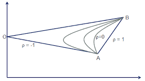
We now examine the other extreme: two assets that move perfectly together but in exactly opposite directions. In this case the standard deviation of the portfolio is [from Equation $(5.4)$ with $\rho=-1.0]$
$$
\sigma_P=\left[X_C^2 \sigma_C^2+\left(1-X_C\right)^2 \sigma_S^2-2 X_C\left(1-X_C\right) \sigma_C \sigma_S\right]^{1 / 2}
$$
Once again, the equation for standard deviation can be simplified. The term in the brackets is equivalent to either of the following two expressions:
$$
\left[X_C \sigma_C-\left(1-X_C\right) \sigma_S\right]^2
$$
or
$$
\left[-X_C \sigma_C+\left(1-X_C\right) \sigma_S\right]^2
$$
Thus $\sigma_P$ is either
$$
\sigma_P=X_C \sigma_C-\left(1-X_C\right) \sigma_S
$$
or
$$
\sigma_P=-X_C \sigma_C+\left(1-X_C\right) \sigma_S
$$
Because we took the square root to obtain an expression for $\sigma_P$ and because the square root of a negative number is imaginary, either of the preceding equations holds only when its right-hand side is positive. A further examination shows that the right-hand side of one equation is simply -1 times the other. Thus each equation is valid only when the righthand side is positive. Because one is always positive when the other is negative (except when both equations equal zero), there is a unique solution for the return and risk of any combination of securities $C$ and $S$. These equations are very similar to the ones we obtained when we had a correlation of +1 . Each also plots as a straight line when $\sigma_P$ is plotted against $X_C$. Thus one would suspect that an examination of the return on the portfolio of two assets as a function of the standard deviation would yield two straight lines, one for each expression for $\sigma_P$. As we observe in a moment, this is, in fact, the case. 5
The value of $\sigma_P$ for Equation (5.7) or (5.8) is always smaller than the value of $\sigma_P$ for the case where $\rho=+1$ [Equation (5.5)] for all values of $X_C$ between 0 and 1 . Thus the risk on a portfolio of assets is always smaller when the correlation coefficient is -1 than when it is +1 . We can go one step further. If two securities are perfectly negatively correlated (i.e., they move in exactly opposite directions), it should always be possible to find some combination of these two securities that has zero risk. By setting either Equation (5.7) or (5.8) equal to 0 , we find that a portfolio with $X_C=\sigma_S /\left(\sigma_S+\sigma_C\right)$ will have zero risk. Because $\sigma_S>0$ and $\sigma_S+\sigma_C>\sigma_S$, this implies that $0<X_C<1$ or that the zero-risk portfolio will always involve positive investment in both securities.

金融代写|利率理论代写portfolio theory代考|Case 4—Intermediate Risk

The correlation between any two actual stocks is almost always greater than 0 and considerably less than 1 . To show a more typical relationship between risk and return for two stocks, we have chosen to examine the relationship when $\rho=+0.5$.

The equation for the risk of portfolios composed of Colonel Motors and Separated Edison when the correlation is 0.5 is
$$
\begin{aligned}
\sigma_P & =\left[(6)^2 X_C^2+(3)^2\left(1-X_C\right)^2+2 X_C\left(1-X_C\right)(3)(6)\left(\frac{1}{2}\right)\right]^{1 / 2} \
\sigma_P & =\left(27 X_C^2+9\right)^{1 / 2}
\end{aligned}
$$
Table 5.4 presents the returns and risks on alternative portfolios of our two stocks when the correlation between them is 0.5 .

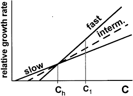
This risk-return relationship is plotted in Figure 5.5 along with the risk-return relationships for other intermediate values of the correlation coefficient. Notice that in this example, if $\rho=0.5$, then the minimum risk is obtained at a value of $X_C=0$ or where the investor has placed $100 \%$ of his funds in Separated Edison. This point could have been derived analytically from Equation (5.9). Employing this equation yields
$$
X_C=\frac{9-18(0.5)}{9+36-2(18)(0.5)}=0
$$
In this example (i.e., $\rho_{C S}=0.5$ ), there is no combination of the two securities that is less risky than the least risky asset by itself, though combinations are still less risky than they were in the case of perfect positive correlation. The particular value of the correlation coefficient for which no combination of two securities is less risky than the least risky security depends on the characteristics of the assets in question. Specifically, for all assets, there is some value of $\rho$ such that the risk of the portfolio can no longer be made less than the risk of the least risky asset in the portfolio. ${ }^7$

We have developed some insights into combinations of two securities or portfolios from the analysis performed to this point. First, we have noted that the lower (closer to -1.0 ) the correlation coefficient between assets, all other attributes held constant, the higher the payoff from diversification. Second, we have seen that combinations of two assets can never have more risk than that found on a straight line connecting the two assets in expected return standard deviation space. Finally, we have produced a simple expression for finding the minimum variance portfolio when two assets are combined in a portfolio. We can use this to gain more insight into the shape of the curve along which all possible combinations of assets must lie in expected return standard deviation space. This curve, which is called the portfolio possibilities curve, is the subject of the next section.

利率理论代考

金融代写|利率理论代写portfolio theory代考|Case 2—Perfect Negative Correlation

我们现在研究另一个极端: 两种资产完美地一起移动,但方向完全相反。在这种情况下,投资组合的标 准差是[来自等式 (5.4)和 $\rho=-1.0]$
$$
\sigma_P=\left[X_C^2 \sigma_C^2+\left(1-X_C\right)^2 \sigma_S^2-2 X_C\left(1-X_C\right) \sigma_C \sigma_S\right]^{1 / 2}
$$
再一次,可以简化标准偏差的方程式。括号中的术语等同于以下两个表达式之一:
$$
\left[X_C \sigma_C-\left(1-X_C\right) \sigma_S\right]^2
$$
或者
$$
\left[-X_C \sigma_C+\left(1-X_C\right) \sigma_S\right]^2
$$
因此 $\sigma_P$ 或者是
$$
\sigma_P=X_C \sigma_C-\left(1-X_C\right) \sigma_S
$$
或者
$$
\sigma_P=-X_C \sigma_C+\left(1-X_C\right) \sigma_S
$$
因为我们取平方根得到一个表达式 $\sigma_P$ 并且因为负数的平方根是虚数,所以只有当其右侧为正时,上述任 一方程式才成立。进一步检查表明,一个方程式的右边只是另一个方程式的 -1 倍。因此,每个等式仅在 右侧为正时才有效。因为当另一个为负时,一个总是正的(除非两个方程都为零),所以对于任何证券 组合的回报和风险都有一个唯一的解决方案 $C$ 和 $S$. 这些方程式与我们在相关性为 +1 时获得的方程式非 常相似。当 $\sigma_P$ 被暗算 $X_C$. 因此,人们会怀疑,将两种资产的投资组合回报率作为标准差的函数进行检查 会产生两条直线,一条直线对应于 $\sigma_P$. 正如我们稍后观察到的,事实确实如此。 5
的价值 $\sigma_P$ 对于等式 (5.7) 或 (5.8) 总是小于的值 $\sigma_P$ 对于这种情况 $\rho=+1$ [等式 (5.5)] 的所有值 $X_C$ 在 0 和 1 之间。因此,当相关系数为 -1 时,资产组合的风险始终小于相关系数为 +1 时的风险。我们可以更 进一步。如果两种证券完全负相关 (即,它们的走势完全相反),则总有可能找到这两种证券的某种零 风险组合。通过将等式 (5.7) 或 (5.8) 设置为 0 ,我们发现一个投资组合 $X_C=\sigma_S /\left(\sigma_S+\sigma_C\right.$ ) 将具有 零风险。因为 $\sigma_S>0$ 和 $\sigma_S+\sigma_C>\sigma_S$, 这意味着 $0<X_C<1$ 或者零风险投资组合将始终涉及对两 种证券的积极投资。

金融代写|利率理论代写portfolio theory代考|Case 4—Intermediate Risk

任何两个实际股票之间的相关性几乎总是大于 0 并且远小于 1。为了显示两只股票的风险和回报之间更 典型的关系,我们选择在以下情况下检查关系 $\rho=+0.5$.
当相关系数为 0.5 时,由 Colonel Motors 和 Separated Edison 组成的投资组合的风险方程为
$$
\sigma_P=\left[(6)^2 X_C^2+(3)^2\left(1-X_C\right)^2+2 X_C\left(1-X_C\right)(3)(6)\left(\frac{1}{2}\right)\right]^{1 / 2} \sigma_P=\left(27 X_C^2+9\right)^{1 / 2}
$$
表 5.4 显示了当它们之间的相关性为 0.5 时,我们两只股票的替代投资组合的回报和风险。
图 5.5 绘制了这种风险回报关系以及相关系数其他中间值的风险回报关系。请注意,在这个例子中,如 果 $\rho=0.5$ ,那么最小风险值是 $X_C=0$ 或投资者放置的地方 $100 \%$ 他在分离爱迪生的资金。这一点可以 从公式 (5.9) 中分析得出。使用这个等式产生
$$
X_C=\frac{9-18(0.5)}{9+36-2(18)(0.5)}=0
$$
在这个例子中 (即 $\rho_{C S}=0.5$ ), 没有两种证券的组合比风险最小的资产本身风险更低,尽管组合的风险 仍然低于完全正相关的情况。两种证券组合的风险都不低于风险最低的证券的相关系数的特定值取决于 相关资产的特征。具体来说,对于所有资产,都有一些价值 $\rho$ 这样投资组合的风险就不能再低于投资组合 中风险最小资产的风险。 ${ }^7$
从执行到现在的分析,我们对两种证券或投资组合的组合有了一些见解。首先,我们注意到资产之间的 相关系数越低 (接近 -1.0),所有其他属性保持不变,多元化的收益就越高。其次,我们已经看到,两 种资产的组合永远不会比在预期收益标准差空间中连接两种资产的直线上发现的风险更大。最后,我们 生成了一个简单的表达式,用于在组合两个资产时找到最小方差组合。我们可以使用它来更深入地了解 曲线的形状,所有可能的资产组合都必须位于预期收益标准差空间中。这条曲线,称为投资组合可能性 曲线,

金融代写|利率理论代写portfolio theory代考 请认准statistics-lab™

统计代写请认准statistics-lab™. statistics-lab™为您的留学生涯保驾护航。

金融工程代写

金融工程是使用数学技术来解决金融问题。金融工程使用计算机科学、统计学、经济学和应用数学领域的工具和知识来解决当前的金融问题,以及设计新的和创新的金融产品。

非参数统计代写

非参数统计指的是一种统计方法,其中不假设数据来自于由少数参数决定的规定模型;这种模型的例子包括正态分布模型和线性回归模型。

广义线性模型代考

广义线性模型(GLM)归属统计学领域,是一种应用灵活的线性回归模型。该模型允许因变量的偏差分布有除了正态分布之外的其它分布。

术语 广义线性模型(GLM)通常是指给定连续和/或分类预测因素的连续响应变量的常规线性回归模型。它包括多元线性回归,以及方差分析和方差分析(仅含固定效应)。

有限元方法代写

有限元方法(FEM)是一种流行的方法,用于数值解决工程和数学建模中出现的微分方程。典型的问题领域包括结构分析、传热、流体流动、质量运输和电磁势等传统领域。

有限元是一种通用的数值方法,用于解决两个或三个空间变量的偏微分方程(即一些边界值问题)。为了解决一个问题,有限元将一个大系统细分为更小、更简单的部分,称为有限元。这是通过在空间维度上的特定空间离散化来实现的,它是通过构建对象的网格来实现的:用于求解的数值域,它有有限数量的点。边界值问题的有限元方法表述最终导致一个代数方程组。该方法在域上对未知函数进行逼近。[1] 然后将模拟这些有限元的简单方程组合成一个更大的方程系统,以模拟整个问题。然后,有限元通过变化微积分使相关的误差函数最小化来逼近一个解决方案。

tatistics-lab作为专业的留学生服务机构,多年来已为美国、英国、加拿大、澳洲等留学热门地的学生提供专业的学术服务,包括但不限于Essay代写,Assignment代写,Dissertation代写,Report代写,小组作业代写,Proposal代写,Paper代写,Presentation代写,计算机作业代写,论文修改和润色,网课代做,exam代考等等。写作范围涵盖高中,本科,研究生等海外留学全阶段,辐射金融,经济学,会计学,审计学,管理学等全球99%专业科目。写作团队既有专业英语母语作者,也有海外名校硕博留学生,每位写作老师都拥有过硬的语言能力,专业的学科背景和学术写作经验。我们承诺100%原创,100%专业,100%准时,100%满意。

随机分析代写


随机微积分是数学的一个分支,对随机过程进行操作。它允许为随机过程的积分定义一个关于随机过程的一致的积分理论。这个领域是由日本数学家伊藤清在第二次世界大战期间创建并开始的。

时间序列分析代写

随机过程,是依赖于参数的一组随机变量的全体,参数通常是时间。 随机变量是随机现象的数量表现,其时间序列是一组按照时间发生先后顺序进行排列的数据点序列。通常一组时间序列的时间间隔为一恒定值(如1秒,5分钟,12小时,7天,1年),因此时间序列可以作为离散时间数据进行分析处理。研究时间序列数据的意义在于现实中,往往需要研究某个事物其随时间发展变化的规律。这就需要通过研究该事物过去发展的历史记录,以得到其自身发展的规律。

回归分析代写

多元回归分析渐进(Multiple Regression Analysis Asymptotics)属于计量经济学领域,主要是一种数学上的统计分析方法,可以分析复杂情况下各影响因素的数学关系,在自然科学、社会和经济学等多个领域内应用广泛。

MATLAB代写

MATLAB 是一种用于技术计算的高性能语言。它将计算、可视化和编程集成在一个易于使用的环境中,其中问题和解决方案以熟悉的数学符号表示。典型用途包括:数学和计算算法开发建模、仿真和原型制作数据分析、探索和可视化科学和工程图形应用程序开发,包括图形用户界面构建MATLAB 是一个交互式系统,其基本数据元素是一个不需要维度的数组。这使您可以解决许多技术计算问题,尤其是那些具有矩阵和向量公式的问题,而只需用 C 或 Fortran 等标量非交互式语言编写程序所需的时间的一小部分。MATLAB 名称代表矩阵实验室。MATLAB 最初的编写目的是提供对由 LINPACK 和 EISPACK 项目开发的矩阵软件的轻松访问,这两个项目共同代表了矩阵计算软件的最新技术。MATLAB 经过多年的发展,得到了许多用户的投入。在大学环境中,它是数学、工程和科学入门和高级课程的标准教学工具。在工业领域,MATLAB 是高效研究、开发和分析的首选工具。MATLAB 具有一系列称为工具箱的特定于应用程序的解决方案。对于大多数 MATLAB 用户来说非常重要,工具箱允许您学习应用专业技术。工具箱是 MATLAB 函数(M 文件)的综合集合,可扩展 MATLAB 环境以解决特定类别的问题。可用工具箱的领域包括信号处理、控制系统、神经网络、模糊逻辑、小波、仿真等。

R语言代写问卷设计与分析代写
PYTHON代写回归分析与线性模型代写
MATLAB代写方差分析与试验设计代写
STATA代写机器学习/统计学习代写
SPSS代写计量经济学代写
EVIEWS代写时间序列分析代写
EXCEL代写深度学习代写
SQL代写各种数据建模与可视化代写

金融代写|利率理论代写portfolio theory代考|Delineating Efficient Portfolios

如果你也在 怎样代写利率理论portfolio theory这个学科遇到相关的难题,请随时右上角联系我们的24/7代写客服。

现代投资组合理论(MPT)指的是一种投资理论,它允许投资者组建一个资产组合,在给定的风险水平下实现预期收益最大化。该理论假设投资者是规避风险的;在给定的预期收益水平下,投资者总是喜欢风险较小的投资组合。

statistics-lab™ 为您的留学生涯保驾护航 在代写利率理论portfolio theory方面已经树立了自己的口碑, 保证靠谱, 高质且原创的统计Statistics代写服务。我们的专家在代写利率理论portfolio theory代写方面经验极为丰富,各种代写利率理论portfolio theory相关的作业也就用不着说。

我们提供的利率理论portfolio theory及其相关学科的代写,服务范围广, 其中包括但不限于:

  • Statistical Inference 统计推断
  • Statistical Computing 统计计算
  • Advanced Probability Theory 高等概率论
  • Advanced Mathematical Statistics 高等数理统计学
  • (Generalized) Linear Models 广义线性模型
  • Statistical Machine Learning 统计机器学习
  • Longitudinal Data Analysis 纵向数据分析
  • Foundations of Data Science 数据科学基础

金融代写|利率理论代写portfolio theory代考|COMBINATIONS OF TWO RISKY ASSETS REVISITED

In Chapter 4 we began the analysis of combinations of risky assets. In this chapter we continue it. Previously, we treated the two assets as if they were individual assets, but nothing in the analysis so constrains them. In fact, when we talk about assets, we could equally well be talking about portfolios of risky assets.

Recall from Chapter 4 that the expected return on a portfolio of two assets is given by
$$
\bar{R}_P=X_A \bar{R}_A+X_B \bar{R}_B
$$
Where
$X_A$ is the fraction of the portfolio held in asset $A$
$X_B$ is the fraction of the portfolio held in asset $B$

$\bar{R}P$ is the expected return on the portfolio $\bar{R}_A$ is the expected return on asset $A$ $\bar{R}_B$ is the expected return on asset $B$ In addition, because we require the investor to be fully invested, the fraction she invests in $A$ plus the fraction she invests in $B$ must equal 1 , or $$ X_A+X_B=1 $$ We can rewrite this expression as $$ X_B=1-X_A $$ Substituting Equation (5.2) into Equation (5.1), we can express the expected return on a portfolio of two assets as $$ \bar{R}_P=X_A \bar{R}_A+\left(1-X_A\right) \bar{R}_B $$ Notice that the expected return on the portfolio is a simple weighted average of the expected returns on the individual securities and that the weights add to 1 . The same is not necessarily true of the risk (standard deviation of the return) of the portfolio. In Chapter 4 the standard deviation of the return on the portfolio was shown to be equal to $$ \sigma_P=\left(X_A^2 \sigma_A^2+X_B^2 \sigma_B^2+2 X_A X_B \sigma{A B}\right)^{1 / 2}
$$

金融代写|利率理论代写portfolio theory代考|Case 1—Perfect Positive Correlation

Let the subscript $C$ stand for Colonel Motors and the subscript $S$ stand for Separated Edison. If the correlation coefficient is +1 , then the equation for the risk on the portfolio, Equation (5.4), simplifies to
$$
\sigma_P=\left[X_C^2 \sigma_C^2+\left(1-X_C\right)^2 \sigma_S^2+2 X_C\left(1-X_C\right) \sigma_C \sigma_S\right]^{1 / 2}
$$
Note that the term in square brackets has the form $X^2+2 X Y+Y^2$ and thus can be written as
$$
\left[X_C \sigma_C+\left(1-X_C\right) \sigma_S\right]^2
$$
Because the standard deviation of the portfolio is equal to the positive square root of this expression, we know that
$$
\sigma_P=X_C \sigma_C+\left(1-X_C\right) \sigma_S
$$
while the expected return on the portfolio is
$$
\bar{R}_P=X_C \bar{R}_C+\left(1-X_C\right) \bar{R}_S
$$
Thus with the correlation coefficient equal to +1 , both risk and return of the portfolio are simply linear combinations of the risk and return of each security. In footnote 3 we show that the form of these two equations means that all combinations of two securities that are perfectly correlated will lie on a straight line in risk and return space. ${ }^3$ We now illustrate that this is true for the stocks in our example. For the two stocks under study,

利率理论代考

金融代写|利率理论代写portfolio theory代考|COMBINATIONS OF TWO RISKY ASSETS REVISITED

在第 4 章中,我们开始分析风险资产的组合。本章我们继续它。以前,我们将这两项资产视为单独的资 产,但分析中没有任何东西会如此限制它们。事实上,当我们谈论资产时,我们同样可以谈论风险资产 的投资组合。
回想一下第 4 章,两种资产组合的预期收益为
$$
\bar{R}_P=X_A \bar{R}_A+X_B \bar{R}_B
$$
在哪里
$X_A$ 是资产中持有的投资组合的一部分 $A$
$X_B$ 是资产中持有的投资组合的一部分 $B$
$\bar{R} P$ 是投资组合的预期回报 $\bar{R}_A$ 是资产的预期回报率 $A \bar{R}_B$ 是资产的预期回报率 $B$ 另外,因为我们要求投 资者全额投资,她投资的那部分 $A$ 加上她投资的部分 $B$ 必须等于 1 ,或者
$$
X_A+X_B=1
$$
我们可以将这个表达式重写为
$$
X_B=1-X_A
$$
将等式 (5.2) 代入等式 (5.1),我们可以将两种资产组合的预期收益表示为
$$
\bar{R}_P=X_A \bar{R}_A+\left(1-X_A\right) \bar{R}_B
$$
请注意,投资组合的预期回报是单个证券的预期回报的简单加权平均值,并且权重相加为 1 。投资组合 的风险 (回报的标准差) 不一定如此。在第 4 章中,投资组合回报率的标准差被证明等于
$$
\sigma_P=\left(X_A^2 \sigma_A^2+X_B^2 \sigma_B^2+2 X_A X_B \sigma A B\right)^{1 / 2}
$$

金融代写|利率理论代写portfolio theory代考|Case 1—Perfect Positive Correlation

让下标 $C$ 代表 Motors 上校和下标 $S$ 代表分离的爱迪生。如果相关系数为 +1 ,则投资组合风险的方程式 (5.4) 简化为
$$
\sigma_P=\left[X_C^2 \sigma_C^2+\left(1-X_C\right)^2 \sigma_S^2+2 X_C\left(1-X_C\right) \sigma_C \sigma_S\right]^{1 / 2}
$$
请注意,方括号中的术语具有以下形式 $X^2+2 X Y+Y^2$ 因此可以写成
$$
\left[X_C \sigma_C+\left(1-X_C\right) \sigma_S\right]^2
$$
因为投资组合的标准差等于这个表达式的正平方根,我们知道
$$
\sigma_P=X_C \sigma_C+\left(1-X_C\right) \sigma_S
$$
而投资组合的预期回报是
$$
\bar{R}_P=X_C \bar{R}_C+\left(1-X_C\right) \bar{R}_S
$$
因此,当相关系数等于 +1 时,投资组合的风险和回报都是每种证券的风险和回报的简单线性组合。在脚 注 3 中,我们表明这两个方程的形式意味着完全相关的两种证券的所有组合将位于风险和收益空间的一 条直线上。 ${ }^3$ 我们现在说明这对我们示例中的股票来说是正确的。对于正在研究的两只股票,

金融代写|利率理论代写portfolio theory代考 请认准statistics-lab™

统计代写请认准statistics-lab™. statistics-lab™为您的留学生涯保驾护航。

金融工程代写

金融工程是使用数学技术来解决金融问题。金融工程使用计算机科学、统计学、经济学和应用数学领域的工具和知识来解决当前的金融问题,以及设计新的和创新的金融产品。

非参数统计代写

非参数统计指的是一种统计方法,其中不假设数据来自于由少数参数决定的规定模型;这种模型的例子包括正态分布模型和线性回归模型。

广义线性模型代考

广义线性模型(GLM)归属统计学领域,是一种应用灵活的线性回归模型。该模型允许因变量的偏差分布有除了正态分布之外的其它分布。

术语 广义线性模型(GLM)通常是指给定连续和/或分类预测因素的连续响应变量的常规线性回归模型。它包括多元线性回归,以及方差分析和方差分析(仅含固定效应)。

有限元方法代写

有限元方法(FEM)是一种流行的方法,用于数值解决工程和数学建模中出现的微分方程。典型的问题领域包括结构分析、传热、流体流动、质量运输和电磁势等传统领域。

有限元是一种通用的数值方法,用于解决两个或三个空间变量的偏微分方程(即一些边界值问题)。为了解决一个问题,有限元将一个大系统细分为更小、更简单的部分,称为有限元。这是通过在空间维度上的特定空间离散化来实现的,它是通过构建对象的网格来实现的:用于求解的数值域,它有有限数量的点。边界值问题的有限元方法表述最终导致一个代数方程组。该方法在域上对未知函数进行逼近。[1] 然后将模拟这些有限元的简单方程组合成一个更大的方程系统,以模拟整个问题。然后,有限元通过变化微积分使相关的误差函数最小化来逼近一个解决方案。

tatistics-lab作为专业的留学生服务机构,多年来已为美国、英国、加拿大、澳洲等留学热门地的学生提供专业的学术服务,包括但不限于Essay代写,Assignment代写,Dissertation代写,Report代写,小组作业代写,Proposal代写,Paper代写,Presentation代写,计算机作业代写,论文修改和润色,网课代做,exam代考等等。写作范围涵盖高中,本科,研究生等海外留学全阶段,辐射金融,经济学,会计学,审计学,管理学等全球99%专业科目。写作团队既有专业英语母语作者,也有海外名校硕博留学生,每位写作老师都拥有过硬的语言能力,专业的学科背景和学术写作经验。我们承诺100%原创,100%专业,100%准时,100%满意。

随机分析代写


随机微积分是数学的一个分支,对随机过程进行操作。它允许为随机过程的积分定义一个关于随机过程的一致的积分理论。这个领域是由日本数学家伊藤清在第二次世界大战期间创建并开始的。

时间序列分析代写

随机过程,是依赖于参数的一组随机变量的全体,参数通常是时间。 随机变量是随机现象的数量表现,其时间序列是一组按照时间发生先后顺序进行排列的数据点序列。通常一组时间序列的时间间隔为一恒定值(如1秒,5分钟,12小时,7天,1年),因此时间序列可以作为离散时间数据进行分析处理。研究时间序列数据的意义在于现实中,往往需要研究某个事物其随时间发展变化的规律。这就需要通过研究该事物过去发展的历史记录,以得到其自身发展的规律。

回归分析代写

多元回归分析渐进(Multiple Regression Analysis Asymptotics)属于计量经济学领域,主要是一种数学上的统计分析方法,可以分析复杂情况下各影响因素的数学关系,在自然科学、社会和经济学等多个领域内应用广泛。

MATLAB代写

MATLAB 是一种用于技术计算的高性能语言。它将计算、可视化和编程集成在一个易于使用的环境中,其中问题和解决方案以熟悉的数学符号表示。典型用途包括:数学和计算算法开发建模、仿真和原型制作数据分析、探索和可视化科学和工程图形应用程序开发,包括图形用户界面构建MATLAB 是一个交互式系统,其基本数据元素是一个不需要维度的数组。这使您可以解决许多技术计算问题,尤其是那些具有矩阵和向量公式的问题,而只需用 C 或 Fortran 等标量非交互式语言编写程序所需的时间的一小部分。MATLAB 名称代表矩阵实验室。MATLAB 最初的编写目的是提供对由 LINPACK 和 EISPACK 项目开发的矩阵软件的轻松访问,这两个项目共同代表了矩阵计算软件的最新技术。MATLAB 经过多年的发展,得到了许多用户的投入。在大学环境中,它是数学、工程和科学入门和高级课程的标准教学工具。在工业领域,MATLAB 是高效研究、开发和分析的首选工具。MATLAB 具有一系列称为工具箱的特定于应用程序的解决方案。对于大多数 MATLAB 用户来说非常重要,工具箱允许您学习应用专业技术。工具箱是 MATLAB 函数(M 文件)的综合集合,可扩展 MATLAB 环境以解决特定类别的问题。可用工具箱的领域包括信号处理、控制系统、神经网络、模糊逻辑、小波、仿真等。

R语言代写问卷设计与分析代写
PYTHON代写回归分析与线性模型代写
MATLAB代写方差分析与试验设计代写
STATA代写机器学习/统计学习代写
SPSS代写计量经济学代写
EVIEWS代写时间序列分析代写
EXCEL代写深度学习代写
SQL代写各种数据建模与可视化代写

统计代写|金融统计代写Financial Statistics代考|GRA6518

如果你也在 怎样代写金融统计Financial Statistics这个学科遇到相关的难题,请随时右上角联系我们的24/7代写客服。

金融统计是将经济物理学应用于金融市场。它没有采用金融学的规范性根源,而是采用实证主义框架。它包括统计物理学的典范,强调金融市场的突发或集体属性。经验观察到的风格化事实是这种理解金融市场的方法的出发点。

statistics-lab™ 为您的留学生涯保驾护航 在代写金融统计Financial Statistics方面已经树立了自己的口碑, 保证靠谱, 高质且原创的统计Statistics代写服务。我们的专家在代写金融统计Financial Statistics代写方面经验极为丰富,各种代写金融统计Financial Statistics相关的作业也就用不着说。

我们提供的金融统计Financial Statistics及其相关学科的代写,服务范围广, 其中包括但不限于:

  • Statistical Inference 统计推断
  • Statistical Computing 统计计算
  • Advanced Probability Theory 高等概率论
  • Advanced Mathematical Statistics 高等数理统计学
  • (Generalized) Linear Models 广义线性模型
  • Statistical Machine Learning 统计机器学习
  • Longitudinal Data Analysis 纵向数据分析
  • Foundations of Data Science 数据科学基础
统计代写|金融统计代写Financial Statistics代考|GRA6518

统计代写|金融统计代写Financial Statistics代考|Probability of Union

To assess the probability of union, first, imagine we randomly select one card from the deck. Let event $A={$ club $}$ and event $B={$ heart or diamond $}$. Let $A \cup B$ denote the union, so $A \cup B={$ club, heart, diamond $}$.

The union of $A$ and $B$ means the event ” $A$ or $B$ ” occurs. We can now compute the mathematical probability of $A$ or $B$ :
$$
P(A)=\frac{13}{52}=\frac{1}{4} \text { and } P(B)=\frac{13+13}{52}=\frac{1}{2}
$$

The probability of getting a club, a heart, or a diamond is obtained by adding the number of club, heart, and diamond cards and dividing by the total number of cards, 52. As a result, the probability of drawing a card that is a member of the union of these two events is
$$
P(A \cup B)=P(A)+P(B)=\frac{1}{4}+\frac{1}{2}=\frac{3}{4}
$$
Thus, we have a $\frac{3}{4}=75 \%$ chance of randomly drawing a single card that is a club or a heart or a diamond.

If $A$ and $B$ are mutually exclusive, the probability formula for a union of $A$ and $B$ is
$$
P(A \cup B)=P(A)+P(B)
$$
The rule for obtaining the probability of the union of $A$ and $B$ as indicated in Eq. $5.4$ is the addition rule for two events that are mutually exclusive. This addition rule is illustrated by the Venn diagram in Fig. 5.9, where we note that the area of two circles taken together (denoting $A \cup B$ ) is the sum of the areas of the two circles.

统计代写|金融统计代写Financial Statistics代考|Probability of Intersection

If $A={$ diamond $}$ and $B={$ diamond or heart $}$, then $A \cap B={$ diamond $}=$ set of points that are in both $A$ and $B$. Using Table 5.2, we obtain
$$
\begin{aligned}
P(A) & =\frac{13}{52}=\frac{1}{4} \
P(B) & =(13+13) / 52=\frac{1}{2} \
P(A \cap B) & =\frac{13}{52}=\frac{1}{4}
\end{aligned}
$$
Thus, the probability of drawing a diamond and drawing a diamond or a heart is the probability of drawing a diamond, which is $\frac{1}{4}$, or $25 \%$.
From Eq. 5.5, we can define the probability of an intersection as
$$
P(A \cap B)=P(A)+P(B)-P(A \cup B)
$$
If, instead, $A=$ all diamonds and $B=$ all diamonds or all hearts, then
$$
P(A \cap B)=\frac{1}{4}+\frac{1}{2}-\frac{1}{2}=\frac{1}{4}
$$

统计代写|金融统计代写Financial Statistics代考|GRA6518

金融统计代考

统计代写|金融统计代写Financial Statistics代考|Probability of Union

为了评估联合的概率,首先,假设我们从一副牌中随机选择一张牌。让事件 $A=\$ c l u b \$$ 和事件 $B=\$$ heartordiamond $\$$. 让 $A \cup B$ 表示并集,所以 $A \cup B=\$ c l u b$, heart, diamond $\$$.
的联盟 $A$ 和 $B$ 表示事件” $A$ 或者 $B^{\prime \prime}$ 发生。我们现在可以计算数学概率 $A$ 或者 $B$ :
$$
P(A)=\frac{13}{52}=\frac{1}{4} \text { and } P(B)=\frac{13+13}{52}=\frac{1}{2}
$$
得到梅花、红桃或方块的概率是将梅花、红心和方块卡的数量相加除以卡片总数 52。因此,抽到卡片的 概率是这两个事件的联合成员是
$$
P(A \cup B)=P(A)+P(B)=\frac{1}{4}+\frac{1}{2}=\frac{3}{4}
$$
因此,我们有一个 $\frac{3}{4}=75 \%$ 随机抽取一张梅花、红心或方块牌的机会。
如果 $A$ 和 $B$ 是互奈的,联合的概率公式 $A$ 和 $B$ 是
$$
P(A \cup B)=P(A)+P(B)
$$
获得并集概率的规则 $A$ 和 $B$ 如方程式所示。5.4是两个互広事件的加法规则。图 $5.9$ 中的维恩图说明了这 个加法规则,我们注意到两个圆的面积合在一起 (表示 $A \cup B)$ 是两个圆的面积之和。

统计代写|金融统计代写Financial Statistics代考|Probability of Intersection

如果 $A=\$$ diamond $\$$ 和 $B=\$$ diamondorheart $\$$ ,然后 $A \cap B=\$$ diamond $\$=$ 两者都存在的 点集 $A$ 和 $B$. 使用表 5.2,我们得到
$$
P(A)=\frac{13}{52}=\frac{1}{4} P(B) \quad=(13+13) / 52=\frac{1}{2} P(A \cap B)=\frac{13}{52}=\frac{1}{4}
$$
于是,抽到钻石的概率和抽到钻石或心形的概率就是抽到钻石的概率,即 $\frac{1}{4}$ ,或者 $25 \%$. 从等式。5.5,我们可以定义相交的概率为
$$
P(A \cap B)=P(A)+P(B)-P(A \cup B)
$$
相反,如果 $A=$ 所有钻石和 $B=$ 所有的钻石或所有的心,那么
$$
P(A \cap B)=\frac{1}{4}+\frac{1}{2}-\frac{1}{2}=\frac{1}{4}
$$

统计代写|金融统计代写Financial Statistics代考 请认准statistics-lab™

统计代写请认准statistics-lab™. statistics-lab™为您的留学生涯保驾护航。

金融工程代写

金融工程是使用数学技术来解决金融问题。金融工程使用计算机科学、统计学、经济学和应用数学领域的工具和知识来解决当前的金融问题,以及设计新的和创新的金融产品。

非参数统计代写

非参数统计指的是一种统计方法,其中不假设数据来自于由少数参数决定的规定模型;这种模型的例子包括正态分布模型和线性回归模型。

广义线性模型代考

广义线性模型(GLM)归属统计学领域,是一种应用灵活的线性回归模型。该模型允许因变量的偏差分布有除了正态分布之外的其它分布。

术语 广义线性模型(GLM)通常是指给定连续和/或分类预测因素的连续响应变量的常规线性回归模型。它包括多元线性回归,以及方差分析和方差分析(仅含固定效应)。

有限元方法代写

有限元方法(FEM)是一种流行的方法,用于数值解决工程和数学建模中出现的微分方程。典型的问题领域包括结构分析、传热、流体流动、质量运输和电磁势等传统领域。

有限元是一种通用的数值方法,用于解决两个或三个空间变量的偏微分方程(即一些边界值问题)。为了解决一个问题,有限元将一个大系统细分为更小、更简单的部分,称为有限元。这是通过在空间维度上的特定空间离散化来实现的,它是通过构建对象的网格来实现的:用于求解的数值域,它有有限数量的点。边界值问题的有限元方法表述最终导致一个代数方程组。该方法在域上对未知函数进行逼近。[1] 然后将模拟这些有限元的简单方程组合成一个更大的方程系统,以模拟整个问题。然后,有限元通过变化微积分使相关的误差函数最小化来逼近一个解决方案。

tatistics-lab作为专业的留学生服务机构,多年来已为美国、英国、加拿大、澳洲等留学热门地的学生提供专业的学术服务,包括但不限于Essay代写,Assignment代写,Dissertation代写,Report代写,小组作业代写,Proposal代写,Paper代写,Presentation代写,计算机作业代写,论文修改和润色,网课代做,exam代考等等。写作范围涵盖高中,本科,研究生等海外留学全阶段,辐射金融,经济学,会计学,审计学,管理学等全球99%专业科目。写作团队既有专业英语母语作者,也有海外名校硕博留学生,每位写作老师都拥有过硬的语言能力,专业的学科背景和学术写作经验。我们承诺100%原创,100%专业,100%准时,100%满意。

随机分析代写


随机微积分是数学的一个分支,对随机过程进行操作。它允许为随机过程的积分定义一个关于随机过程的一致的积分理论。这个领域是由日本数学家伊藤清在第二次世界大战期间创建并开始的。

时间序列分析代写

随机过程,是依赖于参数的一组随机变量的全体,参数通常是时间。 随机变量是随机现象的数量表现,其时间序列是一组按照时间发生先后顺序进行排列的数据点序列。通常一组时间序列的时间间隔为一恒定值(如1秒,5分钟,12小时,7天,1年),因此时间序列可以作为离散时间数据进行分析处理。研究时间序列数据的意义在于现实中,往往需要研究某个事物其随时间发展变化的规律。这就需要通过研究该事物过去发展的历史记录,以得到其自身发展的规律。

回归分析代写

多元回归分析渐进(Multiple Regression Analysis Asymptotics)属于计量经济学领域,主要是一种数学上的统计分析方法,可以分析复杂情况下各影响因素的数学关系,在自然科学、社会和经济学等多个领域内应用广泛。

MATLAB代写

MATLAB 是一种用于技术计算的高性能语言。它将计算、可视化和编程集成在一个易于使用的环境中,其中问题和解决方案以熟悉的数学符号表示。典型用途包括:数学和计算算法开发建模、仿真和原型制作数据分析、探索和可视化科学和工程图形应用程序开发,包括图形用户界面构建MATLAB 是一个交互式系统,其基本数据元素是一个不需要维度的数组。这使您可以解决许多技术计算问题,尤其是那些具有矩阵和向量公式的问题,而只需用 C 或 Fortran 等标量非交互式语言编写程序所需的时间的一小部分。MATLAB 名称代表矩阵实验室。MATLAB 最初的编写目的是提供对由 LINPACK 和 EISPACK 项目开发的矩阵软件的轻松访问,这两个项目共同代表了矩阵计算软件的最新技术。MATLAB 经过多年的发展,得到了许多用户的投入。在大学环境中,它是数学、工程和科学入门和高级课程的标准教学工具。在工业领域,MATLAB 是高效研究、开发和分析的首选工具。MATLAB 具有一系列称为工具箱的特定于应用程序的解决方案。对于大多数 MATLAB 用户来说非常重要,工具箱允许您学习应用专业技术。工具箱是 MATLAB 函数(M 文件)的综合集合,可扩展 MATLAB 环境以解决特定类别的问题。可用工具箱的领域包括信号处理、控制系统、神经网络、模糊逻辑、小波、仿真等。

R语言代写问卷设计与分析代写
PYTHON代写回归分析与线性模型代写
MATLAB代写方差分析与试验设计代写
STATA代写机器学习/统计学习代写
SPSS代写计量经济学代写
EVIEWS代写时间序列分析代写
EXCEL代写深度学习代写
SQL代写各种数据建模与可视化代写

统计代写|金融统计代写Financial Statistics代考|AEM4070

如果你也在 怎样代写金融统计Financial Statistics这个学科遇到相关的难题,请随时右上角联系我们的24/7代写客服。

金融统计是将经济物理学应用于金融市场。它没有采用金融学的规范性根源,而是采用实证主义框架。它包括统计物理学的典范,强调金融市场的突发或集体属性。经验观察到的风格化事实是这种理解金融市场的方法的出发点。

statistics-lab™ 为您的留学生涯保驾护航 在代写金融统计Financial Statistics方面已经树立了自己的口碑, 保证靠谱, 高质且原创的统计Statistics代写服务。我们的专家在代写金融统计Financial Statistics代写方面经验极为丰富,各种代写金融统计Financial Statistics相关的作业也就用不着说。

我们提供的金融统计Financial Statistics及其相关学科的代写,服务范围广, 其中包括但不限于:

  • Statistical Inference 统计推断
  • Statistical Computing 统计计算
  • Advanced Probability Theory 高等概率论
  • Advanced Mathematical Statistics 高等数理统计学
  • (Generalized) Linear Models 广义线性模型
  • Statistical Machine Learning 统计机器学习
  • Longitudinal Data Analysis 纵向数据分析
  • Foundations of Data Science 数据科学基础
统计代写|金融统计代写Financial Statistics代考|AEM4070

统计代写|金融统计代写Financial Statistics代考|Probabilities of Outcomes

The probability of an event is ā real number on a scale from 0 to 1 thât measures the likelihood of the event’s occurring. If an outcome (or event) has a probability of 0 , then its occurrence is impossible; if an outcome (or event) has a probability of 1.0, then its occurrence is certain. Getting either a head or a tail in a coin toss is an example of an event that has a probability of $1.0$. Because there are only two possibilities, either one event or the other is certain to occur. An event with a zero probability is an impossible event, such as getting both a head and a tail when tossing a coin once.

When we roll a fair die, we are just as likely to obtain any face of the die as any other. Because there are six faces to a die, we generally say the “outcome” of the toss can be one of six numbers: $1,2,3,4,5,6$.

The probability of an outcome can be calculated by the classical approach, the relative frequency approach, or the subjective approach. The first two approaches are discussed in this section, the third approach in the next.

Classical probability is often called a priori probability, because if we keep using orderly examples, such as fair coins and unbiased dice, we can state the answer in advance (a priori) without tossing a coin or rolling a die. In other words, we can make statements based on logical reasoning before any experiments take place. Classical probability defines the probability that an event will occur as
$$
\text { Probability of an event }=\frac{\text { number of outcomes containéd in the event }}{\text { total number of possible outcomes }}
$$
Note that this approach is applicable only when all basic outcomes in the sample space are equally probable.
For example, the probability of getting a tail upon tossing a fair coin is
$$
P(\text { tail })=\frac{1}{1+1}=\frac{1}{2}
$$

And for the die-rolling example, the probability of obtaining the face 4 is
$$
P(4)=\frac{1}{6}
$$
The relative frequency approach to calculating probability requires the random experiment to take place as defined in Eq. 5.2:
$$
P\left(o=e_i\right)=\frac{n_i}{N} \quad \text { or } \quad P\left(e_i\right)=\frac{n_i}{N}
$$

统计代写|金融统计代写Financial Statistics代考|Subjective Probability

An alternative view about probability, which does not depend on the concept of repeatable random experiments, defines probability in terms of a subjective, or personalistic, concept. According to this concept of subjective probability, the probability of an event is the degree of belief, or degree of confidence, an individual places in the occurrence of an event on the basis of whatever evidence is available. This evidence may be data on the relative frequency of past occurrences, or it may be just an educated guess. The individual may assign an event the probability of 1 , 0 , or any other number between those two. Here are a few examples of situations that require a subjective probability:

  1. An individual consumer assigns a probability to the event of purchasing a TV during the next quarter.
  2. A quality control manager asserts the probability that a future incoming shipment will have $1.5 \%$ or fewer defective items.
  3. An auditing firm wishes to determine the probability that an audited voucher will contain an error.
  4. An investor ponders the probability that the Dow Jones closing index will be below 3,000 at some time during a 3-month period beginning on November 10, 1992.

As we have stated, an event is the result of a random experiment consisting of one or more basic outcomes. If an event consists of only one basic outcome, it is a simple event; if it consists of more than one basic outcome, it is a composite event. In the die-rolling experiment discussed in Fig. 5.1, the sample space is $S={1,2,3$, $4,5,6}$

Suppose we are interested in the event $E$, where the outcome is 1 or 6 . We can clearly describe the event $E$ as $E={1.6}$. An event $E$ is a subset of the sample space $S$. This is a composite event because it includes the simple events ${1}$ and ${6}$. The subset definition enables us to define an event in general.

In the tossing of a fair die, suppose that event $A$ represents the faces $1,2,3,4$, and 5 and event $B$ the faces of 4,5 , and 6 . Graphically, the relationship between basic outcomes and events can be represented as shown in Fig. 5.6. The intersection of these two events is the faces 4 and 5 , because these faces are common to both events.

统计代写|金融统计代写Financial Statistics代考|AEM4070

金融统计代考

统计代写|金融统计代写Financial Statistics代考|Probabilities of Outcomes

事件的概率是 0 到 1 范围内的实数,用于衡量事件发生的可能性。如果一个结果 (或事件) 的概率为 0 ,那么它的发生是不可能的;如果结果 (或事件) 的概率为 1.0,则它的发生是确定的。在抛硬币中获得 正面或反面是具有概率的事件的示例1.0. 因为只有两种可能性,一个事件或另一个事件肯定会发生。零 概率的事件就是不可能的事件,比如抛一次硬币既得到正面又出现反面。
当我们掷出一个公平的骰子时,我们得到骰子的任何一面的可能性与获得任何其他面的可能性一样。因为 一个骰子有六个面,所以我们通常说郑的”结果”可以是六个数字之一: $1,2,3,4,5,6$.
可以通过经典方法、相对频率方法或主观方法计算结果的概率。本节讨论前两种方法,下一节讨论第三种 方法。
经典概率通常称为先验概率,因为如果我们继续使用有序示例,例如公平硬币和无偏骰子,我们可以预先 (先验) 陈述答案,而无需抛硬币或郱骰子。换句话说,我们可以在进行任何实验之前根据逻辑推理做出 陈述。经典概率将事件发生的概率定义为
$$
\text { Probability of an event }=\frac{\text { number of outcomes containéd in the event }}{\text { total number of possible outcomes }}
$$
请注意,此方法仅适用于样本空间中所有基本结果均等可能的情况。 例如,抛一枚均匀的硬币得到反面的概率是
$$
P(\text { tail })=\frac{1}{1+1}=\frac{1}{2}
$$
而对于郑骰子的例子,得到面 4 的概率是
$$
P(4)=\frac{1}{6}
$$
计算概率的相对频率方法要求进行随机实验,如等式 1 中所定义。5.2:
$$
P\left(o=e_i\right)=\frac{n_i}{N} \quad \text { or } \quad P\left(e_i\right)=\frac{n_i}{N}
$$

统计代写|金融统计代写Financial Statistics代考|Subjective Probability

关于概率的另一种观点不依赖于可重复随机实验的概念,它根据主观或个人主义的概念来定义概率。根据 主观概率的概念,事件的概率是个人根据任何可用证据对事件发生的相信程度或置信度。这个证据可能是 关于过去发生的相对频率的数据,或者它可能只是一个有根据的猜测。个人可以为事件分配 $1 、 0$ 或这 两者之间的任何其他数字的概率。以下是一些需要主观概率的情况示例:

  1. 单个消费者为下一季度购买电视的事件分配概率。
  2. 质量控制经理断言末来进货的可能性 $1.5 \%$ 或更少的次品。
  3. 一家审计公司希望确定经过审计的凭证包含错误的概率。
  4. 一位投资者考虑道琼斯收盘指数在 1992 年 11 月 10 日开始的 3 个月期间的某个时候低于 3,000 的 可能性。
    正如我们所说,事件是由一个或多个基本结果组成的随机实验的结果。如果一个事件只包含一个基本结 果,那么它就是一个简单事件;如果它包含一个以上的基本结果,它就是一个复合事件。在图 $5.1$ 中讨论 的滚模实验中,样本空间为 $S=1,2,3 \$, \$ 4,5,6$
    假设我们对事件感兴趣 $E$ ,其中结果为 1 或 6 。我们可以清楚地描述事件 $E$ 作为 $E=1.6$. 一事件 $E$ 是 样本空间的子集 $S$. 这是一个复合事件,因为它包括简单事件 1 和6. 子集定义使我们能够定义一般事件。
    在公平掷骰子的过程中,假设该事件 $A$ 代表面孔 $1,2,3,4$ ,和 5 和事件 $B 4,5$ 和 6 的面孔。在图形上,基 本结果和事件之间的关系可以用图 $5.6$ 表示。这两个事件的交集是面 4 和 5 ,因为这些面是两个事件共有 的。
统计代写|金融统计代写Financial Statistics代考 请认准statistics-lab™

统计代写请认准statistics-lab™. statistics-lab™为您的留学生涯保驾护航。

金融工程代写

金融工程是使用数学技术来解决金融问题。金融工程使用计算机科学、统计学、经济学和应用数学领域的工具和知识来解决当前的金融问题,以及设计新的和创新的金融产品。

非参数统计代写

非参数统计指的是一种统计方法,其中不假设数据来自于由少数参数决定的规定模型;这种模型的例子包括正态分布模型和线性回归模型。

广义线性模型代考

广义线性模型(GLM)归属统计学领域,是一种应用灵活的线性回归模型。该模型允许因变量的偏差分布有除了正态分布之外的其它分布。

术语 广义线性模型(GLM)通常是指给定连续和/或分类预测因素的连续响应变量的常规线性回归模型。它包括多元线性回归,以及方差分析和方差分析(仅含固定效应)。

有限元方法代写

有限元方法(FEM)是一种流行的方法,用于数值解决工程和数学建模中出现的微分方程。典型的问题领域包括结构分析、传热、流体流动、质量运输和电磁势等传统领域。

有限元是一种通用的数值方法,用于解决两个或三个空间变量的偏微分方程(即一些边界值问题)。为了解决一个问题,有限元将一个大系统细分为更小、更简单的部分,称为有限元。这是通过在空间维度上的特定空间离散化来实现的,它是通过构建对象的网格来实现的:用于求解的数值域,它有有限数量的点。边界值问题的有限元方法表述最终导致一个代数方程组。该方法在域上对未知函数进行逼近。[1] 然后将模拟这些有限元的简单方程组合成一个更大的方程系统,以模拟整个问题。然后,有限元通过变化微积分使相关的误差函数最小化来逼近一个解决方案。

tatistics-lab作为专业的留学生服务机构,多年来已为美国、英国、加拿大、澳洲等留学热门地的学生提供专业的学术服务,包括但不限于Essay代写,Assignment代写,Dissertation代写,Report代写,小组作业代写,Proposal代写,Paper代写,Presentation代写,计算机作业代写,论文修改和润色,网课代做,exam代考等等。写作范围涵盖高中,本科,研究生等海外留学全阶段,辐射金融,经济学,会计学,审计学,管理学等全球99%专业科目。写作团队既有专业英语母语作者,也有海外名校硕博留学生,每位写作老师都拥有过硬的语言能力,专业的学科背景和学术写作经验。我们承诺100%原创,100%专业,100%准时,100%满意。

随机分析代写


随机微积分是数学的一个分支,对随机过程进行操作。它允许为随机过程的积分定义一个关于随机过程的一致的积分理论。这个领域是由日本数学家伊藤清在第二次世界大战期间创建并开始的。

时间序列分析代写

随机过程,是依赖于参数的一组随机变量的全体,参数通常是时间。 随机变量是随机现象的数量表现,其时间序列是一组按照时间发生先后顺序进行排列的数据点序列。通常一组时间序列的时间间隔为一恒定值(如1秒,5分钟,12小时,7天,1年),因此时间序列可以作为离散时间数据进行分析处理。研究时间序列数据的意义在于现实中,往往需要研究某个事物其随时间发展变化的规律。这就需要通过研究该事物过去发展的历史记录,以得到其自身发展的规律。

回归分析代写

多元回归分析渐进(Multiple Regression Analysis Asymptotics)属于计量经济学领域,主要是一种数学上的统计分析方法,可以分析复杂情况下各影响因素的数学关系,在自然科学、社会和经济学等多个领域内应用广泛。

MATLAB代写

MATLAB 是一种用于技术计算的高性能语言。它将计算、可视化和编程集成在一个易于使用的环境中,其中问题和解决方案以熟悉的数学符号表示。典型用途包括:数学和计算算法开发建模、仿真和原型制作数据分析、探索和可视化科学和工程图形应用程序开发,包括图形用户界面构建MATLAB 是一个交互式系统,其基本数据元素是一个不需要维度的数组。这使您可以解决许多技术计算问题,尤其是那些具有矩阵和向量公式的问题,而只需用 C 或 Fortran 等标量非交互式语言编写程序所需的时间的一小部分。MATLAB 名称代表矩阵实验室。MATLAB 最初的编写目的是提供对由 LINPACK 和 EISPACK 项目开发的矩阵软件的轻松访问,这两个项目共同代表了矩阵计算软件的最新技术。MATLAB 经过多年的发展,得到了许多用户的投入。在大学环境中,它是数学、工程和科学入门和高级课程的标准教学工具。在工业领域,MATLAB 是高效研究、开发和分析的首选工具。MATLAB 具有一系列称为工具箱的特定于应用程序的解决方案。对于大多数 MATLAB 用户来说非常重要,工具箱允许您学习应用专业技术。工具箱是 MATLAB 函数(M 文件)的综合集合,可扩展 MATLAB 环境以解决特定类别的问题。可用工具箱的领域包括信号处理、控制系统、神经网络、模糊逻辑、小波、仿真等。

R语言代写问卷设计与分析代写
PYTHON代写回归分析与线性模型代写
MATLAB代写方差分析与试验设计代写
STATA代写机器学习/统计学习代写
SPSS代写计量经济学代写
EVIEWS代写时间序列分析代写
EXCEL代写深度学习代写
SQL代写各种数据建模与可视化代写

统计代写|金融统计代写Financial Statistics代考|ST326

如果你也在 怎样代写金融统计Financial Statistics这个学科遇到相关的难题,请随时右上角联系我们的24/7代写客服。

金融统计是将经济物理学应用于金融市场。它没有采用金融学的规范性根源,而是采用实证主义框架。它包括统计物理学的典范,强调金融市场的突发或集体属性。经验观察到的风格化事实是这种理解金融市场的方法的出发点。

statistics-lab™ 为您的留学生涯保驾护航 在代写金融统计Financial Statistics方面已经树立了自己的口碑, 保证靠谱, 高质且原创的统计Statistics代写服务。我们的专家在代写金融统计Financial Statistics代写方面经验极为丰富,各种代写金融统计Financial Statistics相关的作业也就用不着说。

我们提供的金融统计Financial Statistics及其相关学科的代写,服务范围广, 其中包括但不限于:

  • Statistical Inference 统计推断
  • Statistical Computing 统计计算
  • Advanced Probability Theory 高等概率论
  • Advanced Mathematical Statistics 高等数理统计学
  • (Generalized) Linear Models 广义线性模型
  • Statistical Machine Learning 统计机器学习
  • Longitudinal Data Analysis 纵向数据分析
  • Foundations of Data Science 数据科学基础
统计代写|金融统计代写Financial Statistics代考|ST326

统计代写|金融统计代写Financial Statistics代考|Random Experiment, Outcomes, Sample Space

A random experiment is a process that has at least two possible outcomes and is characterized by uncertainty as to which will occur.
Each of the following examples involves a random experiment:

  1. A die is rolled.
  2. A voter is asked which of four candidates he or she prefers.
  3. A person is asked whether President Bush should order US troops to liberate Kuwait.
  4. The daily change in the price of silver per ounce is observed.
    When a die is rolled, the set of basic outcomes comprises 1 through 6; these basic outcomes represent the various possibilities that can occur. In other words, the possible outcomes of a random experiment are called the basic outcomes. The set of all basic outcomes is called the sample space. Thus, basic outcomes are equivalent to sample points in a sample space.

Suppose you are interested in getting an even number in rolling a die; in this case, the event is rolling a 2,4 , or 6 , which is a subset of ${1,2,3.4,5,6}$. In other words, an event is a set of basic outcomes from the sample space, and it is said to occur if the random experiment gives rise to one of its constituent basic outcomes. Each basic outcome within each event (e.g., ${2}{4}{6}$ ) can also be called a simple event. Hence, an event is a collection of one or more simple events. Finally, a basic event is a subset of the sample space. The concepts of random experiment, outcomes, sample space, and event, then, are fundamental to an understanding of probability.

The starting point of probability is the random experiment. Random experiments have three properties:

  1. They can be repeated physically or conceptually.
  2. The set consisting of all of possible outcomes – that is, the sample space-can be specified in advance.
  3. Various repetitions do not always yield the same outcome.
    Simple examples of conducting a random experiment include rolling dice, tossing a coin, and drawing a card from a deck of 52 playing cards.

Because of uncertainty in the business environment, business decision making is a tricky and an important skill. If the executive knew the exact outcomes of the courses of action available, he or she would have no difficulty making optimal decisions. However, the executive generally does not know the exact outcome of a decision. Thus, business executives spend much time evaluating the probabilities of various alternative outcomes. For example, an executive may need to determine the probability of extensive employee turnover if the firm moves to another area. Or a business decision maker may want to evaluate the impact of changes in economic indicators such as interest rate, inflation, and gross national product (GNP) on a company’s future earnings.

统计代写|金融统计代写Financial Statistics代考|Sample Space of an Experiment and the Venn Diagram

For convenience, we can represent each outcome of a random experiment by a set of symbols. The symbol $S$ is used to represent the sample space of the experiment. As we have noted, the sample space is the set of all basic outcomes (simple events) of the random experiment. In the foregoing die-rolling example, the sample space is $S={1,2,3,4,5,6}$. When a person takes a driver’s license test, the sample space contains only two elements: $S={P, F}$, where $P$ indicates a pass and $F$ a failure. In a stock price forecast, the sample space could contain three elements: $S={U, D$, $N}$, where $U, D$, and $N$ represent movement up, movement down, and no change in the price of a stock. In sum, the different basic outcomes of an experiment are often referred to as sample points (simple events), and the set of all possible outcomes is called the sample space. Thus, the sample points (simple events) form the sample space.

A Venn diagram can be used to describe graphically various basic outcomes (simple events) in a sample space. The rectangle represents the sample space, and the points are basic outcomes. Events are usually represented by circles or rectangles. Figure $5.1$ shows a Venn diagram. The elements labeled represent the six basic outcomes of rolling a die. In Fig. 5.2, the circle indicates the event of all even numbers that can result from rolling a single die. Let event $A={2,4,6}$. Again, the sample space is the possible outcomes of rolling a die. Figure $5.3$ shows events $A={1,3}$ and $B={4,5}$. When two events have no basic outcome in common, they are said to be mutually exclusive events. When events have some elements in common, the intersection of the events is the event that consists of the common elements. Say we have one event $A={2,3,4,6}$ and another event $B={2,3,5}$. The intersection of these events is shown in Fig. 5.4. The common elements are 2 and 3 .

统计代写|金融统计代写Financial Statistics代考|ST326

金融统计代考

统计代写|金融统计代写Financial Statistics代考|Random Experiment, Outcomes, Sample Space

随机实验是一个至少有两种可能结果的过程,其特点是不确定会发生哪种结果。
以下每个示例都涉及随机实验:

  1. 掷骰子。
  2. 选民被问到他或她更喜欢四位候选人中的哪一位。
  3. 有人问布什总统是否应该下令美军解放科威特。
  4. 观察每盎司白银价格的每日变化。
    掷骰子时,基本结果集包括 1 到 6;这些基本结果代表了可能发生的各种可能性。换句话说,随机实验的可能结果称为基本结果。所有基本结果的集合称为样本空间。因此,基本结果相当于样本空间中的样本点。

假设您有兴趣在掷骰子时获得偶数;在这种情况下,事件正在滚动 2,4 或 6 ,它是1,2,3.4,5,6. 换句话说,一个事件是样本空间的一组基本结果,如果随机实验产生了其中一个基本结果,则称该事件发生。每个事件中的每个基本结果(例如,246) 也可以称为简单事件。因此,事件是一个或多个简单事件的集合。最后,基本事件是样本空间的子集。因此,随机实验、结果、样本空间和事件的概念是理解概率的基础。

概率的起点是随机实验。随机实验具有三个属性:

  1. 它们可以在物理上或概念上重复。
  2. 包含所有可能结果的集合——即样本空间——可以预先指定。
  3. 不同的重复并不总是产生相同的结果。
    进行随机实验的简单示例包括掷骰子、抛硬币和从一副 52 张扑克牌中抽一张牌。

由于商业环境的不确定性,商业决策是一项棘手且重要的技能。如果行政人员知道可用行动方案的确切结果,他或她就可以毫不费力地做出最佳决策。但是,执行官通常不知道决策的确切结果。因此,企业高管花费大量时间评估各种备选结果的可能性。例如,如果公司搬到另一个地区,高管可能需要确定大量员工流失的可能性。或者,业务决策者可能希望评估利率、通货膨胀和国民生产总值 (GNP) 等经济指标的变化对公司未来收益的影响。

统计代写|金融统计代写Financial Statistics代考|Sample Space of an Experiment and the Venn Diagram

为方便起见,我们可以用一组符号表示随机实验的每个结果。符号小号用来表示实验的样本空间。正如我们所指出的,样本空间是随机实验的所有基本结果(简单事件)的集合。在上述滚模示例中,样本空间为小号=1,2,3,4,5,6. 当一个人参加驾照考试时,样本空间只包含两个元素:小号=P,F, 在哪里P表示通过和F失败。在股票价格预测中,样本空间可以包含三个元素:小号=在,丁$,$否, 在哪里在,丁, 和否代表股票价格上涨、下跌和不变。总之,一个实验的不同基本结果通常被称为样本点(简单事件),所有可能结果的集合称为样本空间。因此,样本点(简单事件)形成了样本空间。

维恩图可用于以图形方式描述样本空间中的各种基本结果(简单事件)。矩形代表样本空间,点是基本结果。事件通常用圆形或矩形表示。数字5.1显示维恩图。标记的元素代表掷骰子的六个基本结果。在图 5.2 中,圆圈表示掷出单个骰子可能产生的所有偶数的事件。让事件A=2,4,6. 同样,样本空间是掷骰子的可能结果。数字5.3显示事件A=1,3和乙=4,5. 当两个事件没有共同的基本结果时,它们被称为互斥事件。当事件具有某些共同元素时,事件的交集就是由共同元素组成的事件。假设我们有一个事件A=2,3,4,6和另一个事件乙=2,3,5. 这些事件的交集如图 5.4 所示。共同的元素是 2 和 3 。

统计代写|金融统计代写Financial Statistics代考 请认准statistics-lab™

统计代写请认准statistics-lab™. statistics-lab™为您的留学生涯保驾护航。

金融工程代写

金融工程是使用数学技术来解决金融问题。金融工程使用计算机科学、统计学、经济学和应用数学领域的工具和知识来解决当前的金融问题,以及设计新的和创新的金融产品。

非参数统计代写

非参数统计指的是一种统计方法,其中不假设数据来自于由少数参数决定的规定模型;这种模型的例子包括正态分布模型和线性回归模型。

广义线性模型代考

广义线性模型(GLM)归属统计学领域,是一种应用灵活的线性回归模型。该模型允许因变量的偏差分布有除了正态分布之外的其它分布。

术语 广义线性模型(GLM)通常是指给定连续和/或分类预测因素的连续响应变量的常规线性回归模型。它包括多元线性回归,以及方差分析和方差分析(仅含固定效应)。

有限元方法代写

有限元方法(FEM)是一种流行的方法,用于数值解决工程和数学建模中出现的微分方程。典型的问题领域包括结构分析、传热、流体流动、质量运输和电磁势等传统领域。

有限元是一种通用的数值方法,用于解决两个或三个空间变量的偏微分方程(即一些边界值问题)。为了解决一个问题,有限元将一个大系统细分为更小、更简单的部分,称为有限元。这是通过在空间维度上的特定空间离散化来实现的,它是通过构建对象的网格来实现的:用于求解的数值域,它有有限数量的点。边界值问题的有限元方法表述最终导致一个代数方程组。该方法在域上对未知函数进行逼近。[1] 然后将模拟这些有限元的简单方程组合成一个更大的方程系统,以模拟整个问题。然后,有限元通过变化微积分使相关的误差函数最小化来逼近一个解决方案。

tatistics-lab作为专业的留学生服务机构,多年来已为美国、英国、加拿大、澳洲等留学热门地的学生提供专业的学术服务,包括但不限于Essay代写,Assignment代写,Dissertation代写,Report代写,小组作业代写,Proposal代写,Paper代写,Presentation代写,计算机作业代写,论文修改和润色,网课代做,exam代考等等。写作范围涵盖高中,本科,研究生等海外留学全阶段,辐射金融,经济学,会计学,审计学,管理学等全球99%专业科目。写作团队既有专业英语母语作者,也有海外名校硕博留学生,每位写作老师都拥有过硬的语言能力,专业的学科背景和学术写作经验。我们承诺100%原创,100%专业,100%准时,100%满意。

随机分析代写


随机微积分是数学的一个分支,对随机过程进行操作。它允许为随机过程的积分定义一个关于随机过程的一致的积分理论。这个领域是由日本数学家伊藤清在第二次世界大战期间创建并开始的。

时间序列分析代写

随机过程,是依赖于参数的一组随机变量的全体,参数通常是时间。 随机变量是随机现象的数量表现,其时间序列是一组按照时间发生先后顺序进行排列的数据点序列。通常一组时间序列的时间间隔为一恒定值(如1秒,5分钟,12小时,7天,1年),因此时间序列可以作为离散时间数据进行分析处理。研究时间序列数据的意义在于现实中,往往需要研究某个事物其随时间发展变化的规律。这就需要通过研究该事物过去发展的历史记录,以得到其自身发展的规律。

回归分析代写

多元回归分析渐进(Multiple Regression Analysis Asymptotics)属于计量经济学领域,主要是一种数学上的统计分析方法,可以分析复杂情况下各影响因素的数学关系,在自然科学、社会和经济学等多个领域内应用广泛。

MATLAB代写

MATLAB 是一种用于技术计算的高性能语言。它将计算、可视化和编程集成在一个易于使用的环境中,其中问题和解决方案以熟悉的数学符号表示。典型用途包括:数学和计算算法开发建模、仿真和原型制作数据分析、探索和可视化科学和工程图形应用程序开发,包括图形用户界面构建MATLAB 是一个交互式系统,其基本数据元素是一个不需要维度的数组。这使您可以解决许多技术计算问题,尤其是那些具有矩阵和向量公式的问题,而只需用 C 或 Fortran 等标量非交互式语言编写程序所需的时间的一小部分。MATLAB 名称代表矩阵实验室。MATLAB 最初的编写目的是提供对由 LINPACK 和 EISPACK 项目开发的矩阵软件的轻松访问,这两个项目共同代表了矩阵计算软件的最新技术。MATLAB 经过多年的发展,得到了许多用户的投入。在大学环境中,它是数学、工程和科学入门和高级课程的标准教学工具。在工业领域,MATLAB 是高效研究、开发和分析的首选工具。MATLAB 具有一系列称为工具箱的特定于应用程序的解决方案。对于大多数 MATLAB 用户来说非常重要,工具箱允许您学习应用专业技术。工具箱是 MATLAB 函数(M 文件)的综合集合,可扩展 MATLAB 环境以解决特定类别的问题。可用工具箱的领域包括信号处理、控制系统、神经网络、模糊逻辑、小波、仿真等。

R语言代写问卷设计与分析代写
PYTHON代写回归分析与线性模型代写
MATLAB代写方差分析与试验设计代写
STATA代写机器学习/统计学习代写
SPSS代写计量经济学代写
EVIEWS代写时间序列分析代写
EXCEL代写深度学习代写
SQL代写各种数据建模与可视化代写

金融代写|金融工程作业代写Financial Engineering代考|BE953

如果你也在 怎样代写金融工程Financial Engineering这个学科遇到相关的难题,请随时右上角联系我们的24/7代写客服。

金融工程是使用数学技术来解决金融问题。金融工程使用计算机科学、统计学、经济学和应用数学领域的工具和知识来解决当前的金融问题,以及设计新的和创新的金融产品。

statistics-lab™ 为您的留学生涯保驾护航 在代写金融工程Financial Engineering方面已经树立了自己的口碑, 保证靠谱, 高质且原创的统计Statistics代写服务。我们的专家在代写金融工程Financial Engineering代写方面经验极为丰富,各种代写金融工程Financial Engineering相关的作业也就用不着说。

我们提供的金融工程Financial Engineering及其相关学科的代写,服务范围广, 其中包括但不限于:

  • Statistical Inference 统计推断
  • Statistical Computing 统计计算
  • Advanced Probability Theory 高等概率论
  • Advanced Mathematical Statistics 高等数理统计学
  • (Generalized) Linear Models 广义线性模型
  • Statistical Machine Learning 统计机器学习
  • Longitudinal Data Analysis 纵向数据分析
  • Foundations of Data Science 数据科学基础
金融代写|金融工程作业代写Financial Engineering代考|BE953

金融代写|金融工程作业代写Financial Engineering代考|Phase Diagrams for Linear Dynamical Systems

The following autonomous linear system is considered
$$
\dot{x}=A x
$$
The eigenvalues of matrix $A$ define the system dynamics. Some terminology associated with fixed points is as follows:

A fixed point for the system of Eq. (1.27) is called hyperbolic if none of the eigenvalues of matrix $A$ has zero real part. A hyperbolic fixed point is called a saddle if some of the eigenvalues of matrix $A$ have real parts greater than zero and the rest of the eigenvalues have real parts less than zero. If all of the eigenvalues have negative real parts then the hyperbolic fixed point is called a stable node or sink. If all of the eigenvalues have positive real parts then the hyperbolic fixed point is called an unstable node or source. If the eigenvalues are purely imaginary then one has an elliptic fixed point which is said to be a center.
Case 1: Both eigenvalues of matrix $A$ are real and unequal, that is $\lambda_1 \neq \lambda_1 \neq 0$. For $\lambda_1<0$ and $\lambda_2<0$ the phase diagram for $z_1$ and $z_2$ is shown in Fig. 1.4. In case that $\lambda_2$ is smaller than $\lambda_1$ the term $e^{\lambda_2 t}$ decays faster than $e^{\lambda_1 t}$. For $\lambda_1>0>\lambda_2$ the phase diagram of Fig. $1.5$ is obtained.

In the latter case there are stable trajectories along eigenvector $v_1$ and unstable trajectories along eigenvector $v_2$ of matrix $A$. The stability point $(0,0)$ is said to be a saddle point.
When $\lambda_1>\lambda_2>0$ then one has the phase diagrams of Fig. 1.6.
Case 2: Complex eigenvalues:
Typical phase diagrams in the case of stable complex eigenvalues are given in Fig. 1.7.
Typical phase diagrams in the case of unstable complex eigenvalues are given in Fig. 1.8.

Typical phase diagrams in the case of imaginary eigenvalues are given in Fig. 1.9.
Case 3: Matrix $A$ has nonzero eigenvalues which are equal to each other. The associated phase diagram is given in Fig. 1.10.

金融代写|金融工程作业代写Financial Engineering代考|Saddle-Node Bifurcations of Fixed Points

The considered dynamical system is given by $\dot{x}=\mu-x^2$. The fixed points of the system result from the condition $\dot{x}=0$ which for $\mu>0$ gives $x^*=\pm \sqrt{\mu}$. The first fixed point $x=\sqrt{\mu}$ is a stable one whereas the second fixed point $x=-\sqrt{\mu}$ is an unstable one. The phase diagram of the system is given in Fig. 1.14. Since there is one stable and one unstable fixed point the associated bifurcation (locus of the fixed points in the phase plane) will be a saddle-node one.

The bifurcations diagram is given next. The diagram shows how the fixed points of the dynamical system vary with respect to the values of parameter $\mu$. In the above case it represents a parabola in the $\mu-x$ plane as shown in Fig. 1.15.

For $\mu>0$ the dynamical system has two fixed points located at $\pm \sqrt{\mu}$. The one fixed point is stable and is associated with the upper branch of the parabola. The other fixed point is unstable and is associated with the lower branch of the parabola. The value $\mu=0$ is considered to be a bifurcation value and the point $(x, \mu)=(0,0)$ is a bifurcation point. This particular type of bifurcation where the one branch is associated with fixed points and the other branch is not associated to any fixed points is known as saddle-node bifurcation.

In pitchfork bifurcations the number of fixed points varies with respect to the values of the bifurcation parameter. The dynamical system $\dot{x}=x\left(\mu-x^2\right)$ is considered. The associated fixed points are found by the condition $\dot{x}=0$. For $\mu<0$ there is one fixed point at zero which is stable. For $\mu=0$ there is still one fixed point at zero which is still stable. For $\mu>0$ there are three fixed points, one at $x=0$, one at $x=+\sqrt{\mu}$ which is stable and one at $x=-\sqrt{\mu}$ which is also stable. The associated phase diagrams and fixed points are presented in Fig. 1.16.

The bifurcations diagram is given next. The diagram shows how the fixed points of the dynamical system vary with respect to the values of parameter $\mu$. In the above case it represents a parabola in the $\mu-x$ plane as shown in Fig. 1.17.

金融代写|金融工程作业代写Financial Engineering代考|BE953

金融工程代写

金融代写|金融工程作业代写Financial Engineering代考|Phase Diagrams for Linear Dynamical Systems

考虑以下自治线性系统
$$
\dot{x}=A x
$$
矩阵的特征值 $A$ 定义系统动力学。与固定点相关的一些术语如下:
方程式系统的固定点。如果没有矩阵的特征值,则 (1.27) 称为双曲线 $A$ 实部为零。如果矩阵的 某些特征值 $A$ 实部大于零,其余特征值的实部小于零。如果所有特征值都具有负实部,则双曲 不动点称为稳定节点或汇点。如果所有特征值都具有正实部,则双曲不动点称为不稳定节点或 源。如果特征值是纯虚数,则有一个椭圆不动点,称为中心。
情况 1: 矩阵的两个特征值 $A$ 是实数且不相等的,即 $\lambda_1 \neq \lambda_1 \neq 0$. 为了 $\lambda_1<0$ 和 $\lambda_2<0$ 的 相图 $z_1$ 和 $z_2$ 如图 $1.4$ 所示。万 $\lambda_2$ 小于 $\lambda_1$ 期限 $e^{\lambda_2 t}$ 衰减得比 $e^{\lambda_1 t}$. 为了 $\lambda_1>0>\lambda_2$ 图的相 图。1.5获得。
在后一种情况下,沿着特征向量有稳定的轨迹 $v_1$ 和沿特征向量的不稳定轨迹 $v_2$ 矩阵的 $A$. 稳定 点 $(0,0)$ 被称为鞍点。
什么时候 $\lambda_1>\lambda_2>0$ 然后是图 $1.6$ 的相图。
情况 2: 复特征值:
图 $1.7$ 给出了稳定复特征值情况下的典型相图。
图 $1.8$ 给出了不稳定复特征值情况下的典型相图。
图 $1.9$ 给出了虚本征值情况下的典型相图。
案例 3: 矩阵 $A$ 具有彼此相等的非零特征值。相关的相图如图 $1.10$ 所示。

金融代写|金融工程作业代写Financial Engineering代考|Saddle-Node Bifurcations of Fixed Points

所考虑的动力系统由下式给出 $\dot{x}=\mu-x^2$. 系统的固定点由条件产生 $\dot{x}=0$ 哪个 $\mu>0$ 给 $x^*=\pm \sqrt{\mu}$. 第一个固定点 $x=\sqrt{\mu}$ 是稳定的,而第二个不动点 $x=-\sqrt{\mu}$ 是一个不稳定 的。系统的相图如图 $1.14$ 所示。由于存在一个稳定不动点和一个不稳定不动点,因此相关的 分叉 (相平面中不动点的轨迹) 将是一个鞍节点分叉。
接下来给出分叉图。该图显示了动力系统的固定点如何随参数值变化 $\mu$. 在上面的例子中,它 代表了一条抛物线 $\mu-x$ 平面如图 $1.15$ 所示。
为了 $\mu>0$ 动力系统有两个固定点位于 $\pm \sqrt{\mu}$. 一个固定点是稳定的并且与抛物线的上分支相 关联。另一个不动点不稳定,与抛物线的下支有关。价值 $\mu=0$ 被认为是一个分叉值和点 $(x, \mu)=(0,0)$ 是分岔点。这种特殊类型的分叉称为鞍节点分叉,其中一个分支与固定点相 关联,而另一个分支不与任何固定点相关联。
在干草叉分叉中,固定点的数量随分叉参数的值而变化。动力系统 $\dot{x}=x\left(\mu-x^2\right)$ 被认为。 关联的固定点由条件找到 $\dot{x}=0$. 为了 $\mu<0$ 零处有一个固定点是稳定的。为了 $\mu=0$ 在零处 仍有一个固定点仍然稳定。为了 $\mu>0$ 有三个固定点,一个在 $x=0$ ,一在 $x=+\sqrt{\mu}$ 这是 稳定的,一个在 $x=-\sqrt{\mu}$ 这也是稳定的。相关的相图和固定点如图 $1.16$ 所示。
接下来给出分叉图。该图显示了动力系统的固定点如何随参数值变化 $\mu$. 在上面的例子中,它 代表了一条抛物线 $\mu-x$ 平面如图 $1.17$ 所示。

金融代写|金融工程作业代写Financial Engineering代考 请认准statistics-lab™

统计代写请认准statistics-lab™. statistics-lab™为您的留学生涯保驾护航。

金融工程代写

金融工程是使用数学技术来解决金融问题。金融工程使用计算机科学、统计学、经济学和应用数学领域的工具和知识来解决当前的金融问题,以及设计新的和创新的金融产品。

非参数统计代写

非参数统计指的是一种统计方法,其中不假设数据来自于由少数参数决定的规定模型;这种模型的例子包括正态分布模型和线性回归模型。

广义线性模型代考

广义线性模型(GLM)归属统计学领域,是一种应用灵活的线性回归模型。该模型允许因变量的偏差分布有除了正态分布之外的其它分布。

术语 广义线性模型(GLM)通常是指给定连续和/或分类预测因素的连续响应变量的常规线性回归模型。它包括多元线性回归,以及方差分析和方差分析(仅含固定效应)。

有限元方法代写

有限元方法(FEM)是一种流行的方法,用于数值解决工程和数学建模中出现的微分方程。典型的问题领域包括结构分析、传热、流体流动、质量运输和电磁势等传统领域。

有限元是一种通用的数值方法,用于解决两个或三个空间变量的偏微分方程(即一些边界值问题)。为了解决一个问题,有限元将一个大系统细分为更小、更简单的部分,称为有限元。这是通过在空间维度上的特定空间离散化来实现的,它是通过构建对象的网格来实现的:用于求解的数值域,它有有限数量的点。边界值问题的有限元方法表述最终导致一个代数方程组。该方法在域上对未知函数进行逼近。[1] 然后将模拟这些有限元的简单方程组合成一个更大的方程系统,以模拟整个问题。然后,有限元通过变化微积分使相关的误差函数最小化来逼近一个解决方案。

tatistics-lab作为专业的留学生服务机构,多年来已为美国、英国、加拿大、澳洲等留学热门地的学生提供专业的学术服务,包括但不限于Essay代写,Assignment代写,Dissertation代写,Report代写,小组作业代写,Proposal代写,Paper代写,Presentation代写,计算机作业代写,论文修改和润色,网课代做,exam代考等等。写作范围涵盖高中,本科,研究生等海外留学全阶段,辐射金融,经济学,会计学,审计学,管理学等全球99%专业科目。写作团队既有专业英语母语作者,也有海外名校硕博留学生,每位写作老师都拥有过硬的语言能力,专业的学科背景和学术写作经验。我们承诺100%原创,100%专业,100%准时,100%满意。

随机分析代写


随机微积分是数学的一个分支,对随机过程进行操作。它允许为随机过程的积分定义一个关于随机过程的一致的积分理论。这个领域是由日本数学家伊藤清在第二次世界大战期间创建并开始的。

时间序列分析代写

随机过程,是依赖于参数的一组随机变量的全体,参数通常是时间。 随机变量是随机现象的数量表现,其时间序列是一组按照时间发生先后顺序进行排列的数据点序列。通常一组时间序列的时间间隔为一恒定值(如1秒,5分钟,12小时,7天,1年),因此时间序列可以作为离散时间数据进行分析处理。研究时间序列数据的意义在于现实中,往往需要研究某个事物其随时间发展变化的规律。这就需要通过研究该事物过去发展的历史记录,以得到其自身发展的规律。

回归分析代写

多元回归分析渐进(Multiple Regression Analysis Asymptotics)属于计量经济学领域,主要是一种数学上的统计分析方法,可以分析复杂情况下各影响因素的数学关系,在自然科学、社会和经济学等多个领域内应用广泛。

MATLAB代写

MATLAB 是一种用于技术计算的高性能语言。它将计算、可视化和编程集成在一个易于使用的环境中,其中问题和解决方案以熟悉的数学符号表示。典型用途包括:数学和计算算法开发建模、仿真和原型制作数据分析、探索和可视化科学和工程图形应用程序开发,包括图形用户界面构建MATLAB 是一个交互式系统,其基本数据元素是一个不需要维度的数组。这使您可以解决许多技术计算问题,尤其是那些具有矩阵和向量公式的问题,而只需用 C 或 Fortran 等标量非交互式语言编写程序所需的时间的一小部分。MATLAB 名称代表矩阵实验室。MATLAB 最初的编写目的是提供对由 LINPACK 和 EISPACK 项目开发的矩阵软件的轻松访问,这两个项目共同代表了矩阵计算软件的最新技术。MATLAB 经过多年的发展,得到了许多用户的投入。在大学环境中,它是数学、工程和科学入门和高级课程的标准教学工具。在工业领域,MATLAB 是高效研究、开发和分析的首选工具。MATLAB 具有一系列称为工具箱的特定于应用程序的解决方案。对于大多数 MATLAB 用户来说非常重要,工具箱允许您学习应用专业技术。工具箱是 MATLAB 函数(M 文件)的综合集合,可扩展 MATLAB 环境以解决特定类别的问题。可用工具箱的领域包括信号处理、控制系统、神经网络、模糊逻辑、小波、仿真等。

R语言代写问卷设计与分析代写
PYTHON代写回归分析与线性模型代写
MATLAB代写方差分析与试验设计代写
STATA代写机器学习/统计学习代写
SPSS代写计量经济学代写
EVIEWS代写时间序列分析代写
EXCEL代写深度学习代写
SQL代写各种数据建模与可视化代写

金融代写|金融工程作业代写Financial Engineering代考|ICEFE2022

如果你也在 怎样代写金融工程Financial Engineering这个学科遇到相关的难题,请随时右上角联系我们的24/7代写客服。

金融工程是使用数学技术来解决金融问题。金融工程使用计算机科学、统计学、经济学和应用数学领域的工具和知识来解决当前的金融问题,以及设计新的和创新的金融产品。

statistics-lab™ 为您的留学生涯保驾护航 在代写金融工程Financial Engineering方面已经树立了自己的口碑, 保证靠谱, 高质且原创的统计Statistics代写服务。我们的专家在代写金融工程Financial Engineering代写方面经验极为丰富,各种代写金融工程Financial Engineering相关的作业也就用不着说。

我们提供的金融工程Financial Engineering及其相关学科的代写,服务范围广, 其中包括但不限于:

  • Statistical Inference 统计推断
  • Statistical Computing 统计计算
  • Advanced Probability Theory 高等概率论
  • Advanced Mathematical Statistics 高等数理统计学
  • (Generalized) Linear Models 广义线性模型
  • Statistical Machine Learning 统计机器学习
  • Longitudinal Data Analysis 纵向数据分析
  • Foundations of Data Science 数据科学基础
金融代写|金融工程作业代写Financial Engineering代考|ICEFE2022

金融代写|金融工程作业代写Financial Engineering代考|Lyapunov Stability Approach

The Lyapunov method analyzes the stability of a dynamical system without the need to compute explicitly the trajectories of the state vector $x=\left[x_1, x_2, \cdots, x_n\right]^T$.
Theorem: The system described by the relation $\dot{x}=f(x)$ is asymptotically stable in the vicinity of the equilibrium $x_0=0$ if there is a function $V(x)$ such that
(i) $V(x)$ to be continuous and to have a continuous first order derivative at $x_0$
(ii) $V(x)>0$ if $x \neq 0$ and $V(0)=0$
(iii) $\dot{V}(x)<0, \forall x \neq 0$.
The Lyapunov function is usually chosen to be a quadratic (and thus positive) energy function of the system however there in no systematic method to define it.

Assume now, that $\dot{x}=f(x)$ and $x_0=0$ is the equilibrium. Then the system is globally asymptotically stable if for every $\varepsilon>0, \exists \delta(\varepsilon)>0$, such that if $|x(0)|<\delta$ then $|x(t)|<\varepsilon, \forall t \geq 0$.

This means that if the state vector of the system starts in a disc of radius $\delta$ then as time advances it will remain in the disc of radius $\varepsilon$, as shown in Fig. 1.3. Moreover, if $\lim _{t \rightarrow \infty}|x(t)|=x_0=0$ then the system is globally asymptotically stable.
Example 1: Consider the system
$$
\begin{gathered}
\dot{x}_1=x_2 \
\dot{x}_2=-x_1-x_3^2
\end{gathered}
$$
The following Lyapunov function is defined
$$
V(x)-x_1^2+x_2^2
$$

The equilibrium point is $\left(x_1=0, x_2=0\right)$. It holds that $V(x)>0 \forall\left(x_1, x_2\right) \neq(0,0)$ and $V(x)=0$ for $\left(x_1, x_2\right)=(0,0)$. Moreover, it holds
$$
\begin{gathered}
\dot{V}(x)=2 x_1 \dot{x}1+2 x_2 \dot{x}_2=2 x_1 x_2+2 x_2\left(-x_1-x_2^3\right) \Rightarrow \ \dot{V}(x)=-2 x_2^4<0 \forall\left(x_1, x_2\right) \neq(0,0) \end{gathered} $$ Therefore, the system is asymptotically stable and $\lim {t \rightarrow \infty}\left(x_1, x_2\right)=(0,0)$.

金融代写|金融工程作业代写Financial Engineering代考|Local Stability Properties of a Nonlinear Model

Local stability of a nonlinear model can be studied round the associated equilibria. Local linearization can be performed round equilibria, using the set of differential equations that describe the nonlinear model $\dot{x}=h(x)$ and performing Taylor series expansion, that is $\dot{x}=h(x) \Rightarrow \dot{x}=\left.h\left(x_0\right)\right|_{x_0}+\nabla_x h\left(x-x_0\right)+\cdots$.
The nonlinear model is taken to have the generic form
$$
\left(\begin{array}{l}
\dot{x}_1 \
\dot{x}_2
\end{array}\right)=\left(\begin{array}{l}
f\left(x_1, x_2\right) \
g\left(x_1, x_2\right)
\end{array}\right)
$$
where $f\left(x_1, x_2\right)=2 x_1+x_2^2$ and $g\left(x_1, x_2\right)=x_1^2+2 x_2$. The fixed points of this model are computed from the condition $\dot{x}_1=0$ and $\dot{x}_2=0$. Using these relations one finds the equilibria $\left(x_1^, x_2^\right)=(0,0)$ and $\left(x_1^, x_2^\right)=(0,0)$
The Jacobian matrix $\nabla_x h=M$ is given by
$$
M=\left(\begin{array}{ll}
\frac{\partial f}{\partial x_1} & \frac{\partial f}{\partial x_2} \
\frac{\partial g}{\partial x_1} & \frac{\partial g}{\partial x_2}
\end{array}\right)
$$
which results into the matrix
$$
J=\left(\begin{array}{cc}
2 & 2 x_2 \
2 x_1 & 2
\end{array}\right)
$$
The eigenvalues of matrix $M$ define stability round fixed points (stable or unstable fixed point). To this end, one has to find the roots of the associated characteristic polynomial that is given by $\operatorname{det}(\lambda I-J)=0$ where $I$ is the identity matrix.

金融代写|金融工程作业代写Financial Engineering代考|ICEFE2022

金融工程代写

金融代写|金融工程作业代写Financial Engineering代考|Lyapunov Stability Approach

Lyapunov 方法分析动力系统的稳定性,无需显式计算状态向量的轨迹
$$
x=\left[x_1, x_2, \cdots, x_n\right]^T \text {. }
$$
定理: 由关系描述的系统 $\dot{x}=f(x)$ 在平衡点附近渐近稳定 $x_0=0$ 如果有函数 $V(x)$ 这样
(i) $V(x)$ 是连续的,并且有一个连续的一阶导数在 $x_0$
(二) $V(x)>0$ 如果 $x \neq 0$ 和 $V(0)=0$
(三) $\dot{V}(x)<0, \forall x \neq 0$. Lyapunov 函数通常被选择为系统的二次 (因此是正) 能量函数,但是没有系统的方法来定义 它。 现在假设, $\dot{x}=f(x)$ 和 $x_0=0$ 是平衡点。那么系统是全局渐近稳定的如果对于每个 $\varepsilon>0, \exists \delta(\varepsilon)>0$, 这样如果 $|x(0)|<\delta$ 然后 $|x(t)|<\varepsilon, \forall t \geq 0$. 这意味着如果系统的状态向量开始于半径为 $\delta$ 然后随着时间的推移它将保留在半径的圆盘中 $\varepsilon$ , 如图1.3所示。此外,如果 $\lim _{t \rightarrow \infty}|x(t)|=x_0=0$ 那么系统是全局渐近稳定的。 示例 1:考虑系统 $$ \dot{x}_1=x_2 \dot{x}_2=-x_1-x_3^2 $$ 定义了以下 Lyapunov 函数 $$ V(x)-x_1^2+x_2^2 $$ 平衡点是 $\left(x_1=0, x_2=0\right)$. 它认为 $V(x)>0 \forall\left(x_1, x_2\right) \neq(0,0)$ 和 $V(x)=0$ 为了 $\left(x_1, x_2\right)=(0,0)$. 此外, 它持有
$$
\dot{V}(x)=2 x_1 \dot{x} 1+2 x_2 \dot{x}_2=2 x_1 x_2+2 x_2\left(-x_1-x_2^3\right) \Rightarrow \dot{V}(x)=-2 x_2^4<0 \forall\left(x_1, x_2\right)
$$
因此,系统斩近稳定且 $\lim t \rightarrow \infty\left(x_1, x_2\right)=(0,0)$.

金融代写|金融工程作业代写Financial Engineering代考|Local Stability Properties of a Nonlinear Model

非线性模型的局部稳定性可以围绕相关平衡进行研究。可以使用描述非线性模型的微分方程组 在循环平衡中执行局部线性化 $\dot{x}=h(x)$ 并进行泰勒级数展开,即 $\dot{x}=h(x) \Rightarrow \dot{x}=\left.h\left(x_0\right)\right|{x_0}+\nabla_x h\left(x-x_0\right)+\cdots$ 非线性模型采用一般形式 $$ \left(\dot{x}_1 \dot{x}_2\right)=\left(f\left(x_1, x_2\right) g\left(x_1, x_2\right)\right) $$ 在哪里 $f\left(x_1, x_2\right)=2 x_1+x_2^2$ 和 $g\left(x_1, x_2\right)=x_1^2+2 x_2$. 该模型的固定点是根据条件计算 的 $\dot{x}_1=0$ 和 $\dot{x}_2=0$. 使用这些关系可以找到平衡点 $\bigcup$ |left $\left(x{-} 1 \wedge, x_{-} 2 \wedge r i g h t\right)=(0,0)$ 和
left $\left(x_{-} 1 \wedge, x_{-} _2 \wedge\right.$ right $)=(0,0)$
雅可比矩阵 $\nabla_x h=M$ 是 (谁) 给的
$$
M=\left(\begin{array}{llll}
\frac{\partial f}{\partial x_1} & \frac{\partial f}{\partial x_2} & \frac{\partial g}{\partial x_1} & \frac{\partial g}{\partial x_2}
\end{array}\right)
$$
结果进入矩阵
$$
J=\left(\begin{array}{lll}
2 & 2 x_2 2 x_1 & 2
\end{array}\right)
$$
矩阵的特征值 $M$ 定义围绕固定点的稳定性 (稳定或不稳定的固定点)。为此,必须找到由下 式给出的相关特征多项式的根 $\operatorname{det}(\lambda I-J)=0$ 在哪里 $I$ 是单位矩阵。

金融代写|金融工程作业代写Financial Engineering代考 请认准statistics-lab™

统计代写请认准statistics-lab™. statistics-lab™为您的留学生涯保驾护航。

金融工程代写

金融工程是使用数学技术来解决金融问题。金融工程使用计算机科学、统计学、经济学和应用数学领域的工具和知识来解决当前的金融问题,以及设计新的和创新的金融产品。

非参数统计代写

非参数统计指的是一种统计方法,其中不假设数据来自于由少数参数决定的规定模型;这种模型的例子包括正态分布模型和线性回归模型。

广义线性模型代考

广义线性模型(GLM)归属统计学领域,是一种应用灵活的线性回归模型。该模型允许因变量的偏差分布有除了正态分布之外的其它分布。

术语 广义线性模型(GLM)通常是指给定连续和/或分类预测因素的连续响应变量的常规线性回归模型。它包括多元线性回归,以及方差分析和方差分析(仅含固定效应)。

有限元方法代写

有限元方法(FEM)是一种流行的方法,用于数值解决工程和数学建模中出现的微分方程。典型的问题领域包括结构分析、传热、流体流动、质量运输和电磁势等传统领域。

有限元是一种通用的数值方法,用于解决两个或三个空间变量的偏微分方程(即一些边界值问题)。为了解决一个问题,有限元将一个大系统细分为更小、更简单的部分,称为有限元。这是通过在空间维度上的特定空间离散化来实现的,它是通过构建对象的网格来实现的:用于求解的数值域,它有有限数量的点。边界值问题的有限元方法表述最终导致一个代数方程组。该方法在域上对未知函数进行逼近。[1] 然后将模拟这些有限元的简单方程组合成一个更大的方程系统,以模拟整个问题。然后,有限元通过变化微积分使相关的误差函数最小化来逼近一个解决方案。

tatistics-lab作为专业的留学生服务机构,多年来已为美国、英国、加拿大、澳洲等留学热门地的学生提供专业的学术服务,包括但不限于Essay代写,Assignment代写,Dissertation代写,Report代写,小组作业代写,Proposal代写,Paper代写,Presentation代写,计算机作业代写,论文修改和润色,网课代做,exam代考等等。写作范围涵盖高中,本科,研究生等海外留学全阶段,辐射金融,经济学,会计学,审计学,管理学等全球99%专业科目。写作团队既有专业英语母语作者,也有海外名校硕博留学生,每位写作老师都拥有过硬的语言能力,专业的学科背景和学术写作经验。我们承诺100%原创,100%专业,100%准时,100%满意。

随机分析代写


随机微积分是数学的一个分支,对随机过程进行操作。它允许为随机过程的积分定义一个关于随机过程的一致的积分理论。这个领域是由日本数学家伊藤清在第二次世界大战期间创建并开始的。

时间序列分析代写

随机过程,是依赖于参数的一组随机变量的全体,参数通常是时间。 随机变量是随机现象的数量表现,其时间序列是一组按照时间发生先后顺序进行排列的数据点序列。通常一组时间序列的时间间隔为一恒定值(如1秒,5分钟,12小时,7天,1年),因此时间序列可以作为离散时间数据进行分析处理。研究时间序列数据的意义在于现实中,往往需要研究某个事物其随时间发展变化的规律。这就需要通过研究该事物过去发展的历史记录,以得到其自身发展的规律。

回归分析代写

多元回归分析渐进(Multiple Regression Analysis Asymptotics)属于计量经济学领域,主要是一种数学上的统计分析方法,可以分析复杂情况下各影响因素的数学关系,在自然科学、社会和经济学等多个领域内应用广泛。

MATLAB代写

MATLAB 是一种用于技术计算的高性能语言。它将计算、可视化和编程集成在一个易于使用的环境中,其中问题和解决方案以熟悉的数学符号表示。典型用途包括:数学和计算算法开发建模、仿真和原型制作数据分析、探索和可视化科学和工程图形应用程序开发,包括图形用户界面构建MATLAB 是一个交互式系统,其基本数据元素是一个不需要维度的数组。这使您可以解决许多技术计算问题,尤其是那些具有矩阵和向量公式的问题,而只需用 C 或 Fortran 等标量非交互式语言编写程序所需的时间的一小部分。MATLAB 名称代表矩阵实验室。MATLAB 最初的编写目的是提供对由 LINPACK 和 EISPACK 项目开发的矩阵软件的轻松访问,这两个项目共同代表了矩阵计算软件的最新技术。MATLAB 经过多年的发展,得到了许多用户的投入。在大学环境中,它是数学、工程和科学入门和高级课程的标准教学工具。在工业领域,MATLAB 是高效研究、开发和分析的首选工具。MATLAB 具有一系列称为工具箱的特定于应用程序的解决方案。对于大多数 MATLAB 用户来说非常重要,工具箱允许您学习应用专业技术。工具箱是 MATLAB 函数(M 文件)的综合集合,可扩展 MATLAB 环境以解决特定类别的问题。可用工具箱的领域包括信号处理、控制系统、神经网络、模糊逻辑、小波、仿真等。

R语言代写问卷设计与分析代写
PYTHON代写回归分析与线性模型代写
MATLAB代写方差分析与试验设计代写
STATA代写机器学习/统计学习代写
SPSS代写计量经济学代写
EVIEWS代写时间序列分析代写
EXCEL代写深度学习代写
SQL代写各种数据建模与可视化代写

金融代写|金融工程作业代写Financial Engineering代考|Best107

如果你也在 怎样代写金融工程Financial Engineering这个学科遇到相关的难题,请随时右上角联系我们的24/7代写客服。

金融工程是使用数学技术来解决金融问题。金融工程使用计算机科学、统计学、经济学和应用数学领域的工具和知识来解决当前的金融问题,以及设计新的和创新的金融产品。

statistics-lab™ 为您的留学生涯保驾护航 在代写金融工程Financial Engineering方面已经树立了自己的口碑, 保证靠谱, 高质且原创的统计Statistics代写服务。我们的专家在代写金融工程Financial Engineering代写方面经验极为丰富,各种代写金融工程Financial Engineering相关的作业也就用不着说。

我们提供的金融工程Financial Engineering及其相关学科的代写,服务范围广, 其中包括但不限于:

  • Statistical Inference 统计推断
  • Statistical Computing 统计计算
  • Advanced Probability Theory 高等概率论
  • Advanced Mathematical Statistics 高等数理统计学
  • (Generalized) Linear Models 广义线性模型
  • Statistical Machine Learning 统计机器学习
  • Longitudinal Data Analysis 纵向数据分析
  • Foundations of Data Science 数据科学基础
金融代写|金融工程作业代写Financial Engineering代考|Best107

金融代写|金融工程作业代写Financial Engineering代考|Characteristics of the Dynamics of Nonlinear Systems

Main features characterizing the stability of nonlinear dynamical systems are defined as follows [121, 274]:

  1. Finite escape time: It is the finite time within which the state-vector of the nonlinear system converges to infinity.
  2. Multiple isolated equilibria: A linear system can have only one equilibrium to which converges the state vector of the system in steady-state. A nonlinear system can have more than one isolated equilibria (fixed points). Depending on the initial state of the system, in steady-state the state vector of the system can converge to one of these equilibria.
  3. Limit cycles: For a linear system to exhibit oscillations it must have eigenvalues on the imaginary axis. The amplitude of the oscillations depends on initial conditions. In nonlinear systems one may have oscillations of constant amplitude and frequency, which do not depend on initial conditions. This type of oscillations is known as limit cycles.
  4. Sub-harmonic, harmonic and almost periodic oscillations: A stable linear system under periodic input produces an output of the same frequency. A nonlinear system,

under periodic excitation can generate oscillations with frequencies which are several times smaller (subharmonic) or multiples of the frequency of the input (harmonic). It may also generate almost periodic oscillations with frequencies which are not necessarily multiples of a basis frequency (almost periodic oscillations).

  1. Chaos: A nonlinear system in steady-state can exhibit a behavior which is not characterized as equilibrium, periodic oscillation or almost periodic oscillation. This behavior is characterized as chaos. As time advances the behavior of the system changes in a random-like manner, and this depends on the initial conditions. Although the dynamic system is deterministic it exhibits randomness in the way it evolves in time.
  2. Multiple modes of behavior: It is possible the same dynamical system to exhibit simultaneously more than one of the aforementioned characteristics (1)-(5). Thus, a system without external excitation may exhibit simultaneously more than one limit cycles. A system receiving a periodic external input may exhibit harmonic or subharmonic oscillations, or an even more complex behavior in steady state which depends on the amplitude and frequency of the excitation.

金融代写|金融工程作业代写Financial Engineering代考|Computation of Isoclines

An autonomous second order system is described by two differential equations of the form
$$
\begin{aligned}
& \dot{x}_1=f_1\left(x_1, x_2\right) \
& \dot{x}_2=f_2\left(x_1, x_2\right)
\end{aligned}
$$
The method of the isoclines consists of computing the slope (ratio) between $f_2$ and $f_1$ for every point of the trajectory of the state vector $\left(x_1, x_2\right)$.
$$
s(x)=\frac{f_2\left(x_1, x_2\right)}{f_1\left(x_1, x_2\right)}
$$
The case $s(x)=c$ describes a curve in the $x_1-x_2$ plane along which the trajectories $\dot{x}_1=f_1\left(x_1, x_2\right)$ and $\dot{x}_2=f_2\left(x_1, x_2\right)$ have a constant slope.

The curve $s(x)=c$ is drawn in the $x_1-x_2$ plane and along this curve one also draws small linear segments of length $c$. The curve $s(x)=c$ is known as isocline. The direction of these small linear segments is according to the sign of the ratio $f_2\left(x_1, x_2\right) / f_1\left(x_1, x_2\right)$.
Example 1:
The following simplified nonlinear dynamical system is considered
$$
\begin{gathered}
\dot{x}_1=x_2 \
\dot{x}_2=-\sin \left(x_1\right)
\end{gathered}
$$

The slope $s(x)$ is given by the relation
$$
s(x)=\frac{f_2\left(x_1, x_2\right)}{f_1\left(x_1, x_2\right)} \Rightarrow s(x)=-\frac{s i n\left(x_2\right)}{x_2}
$$
Setting $s(x)=c$ it holds that the isoclines are given by the relation
$$
x_2=-\frac{1}{c} \sin \left(x_1\right)
$$
For different values of $c$ one has the following isoclines diagram depicted in Fig. 1.1. Example 2:

The following oscillator model is considered, being free of friction and with statespace equations
$$
\begin{gathered}
\dot{x}_1=x_2 \
\dot{x}_2=-0.5 x_2-\sin \left(x_1\right)
\end{gathered}
$$

金融代写|金融工程作业代写Financial Engineering代考|Best107

金融工程代写

金融代写|金融工程作业代写Financial Engineering代考|Characteristics of the Dynamics of Nonlinear Systems

表征非线性动力系统稳定性的主要特征定义如下 [121, 274]:

  1. 有限逃逸时间:是非线性系统的状态向量收敛到无穷大的有限时间。
  2. 多重孤立平衡:一个线性系统只能有一个平衡点,该平衡点收敛于稳态系统的状态向量。一个非线性系统可以有多个孤立的平衡点(不动点)。根据系统的初始状态,在稳态下,系统的状态向量可以收敛到这些平衡点之一。
  3. 极限环:对于表现出振荡的线性系统,它必须在虚轴上具有特征值。振荡的幅度取决于初始条件。在非线性系统中,可能存在幅度和频率恒定的振荡,不依赖于初始条件。这种类型的振荡被称为极限环。
  4. 次谐波、谐波和几乎周期性振荡:在周期性输入下稳定的线性系统会产生相同频率的输出。一个非线性系统,

在周期性激励下会产生频率比输入频率小几倍(次谐波)或数倍(谐波)的振荡。它还可能产生几乎周期性的振荡,其频率不一定是基频的倍数(几乎周期性振荡)。

  1. 混沌:处于稳态的非线性系统可能表现出一种不具有平衡、周期性振荡或几乎周期性振荡特征的行为。这种行为的特点是混乱。随着时间的推移,系统的行为会以类似随机的方式发生变化,这取决于初始条件。尽管动态系统是确定性的,但它随时间演化的方式表现出随机性。
  2. 多种行为模式:同一动力系统可能同时表现出上述特征 (1)-(5) 中的一个以上。因此,没有外部激励的系统可能同时表现出多个极限循环。接收周期性外部输入的系统可能会表现出谐波或次谐波振荡,或者在稳态下表现出更复杂的行为,这取决于激励的幅度和频率。

金融代写|金融工程作业代写Financial Engineering代考|Computation of Isoclines

自治二阶系统由以下形式的两个微分方程描述
$$
\dot{x}_1=f_1\left(x_1, x_2\right) \quad \dot{x}_2=f_2\left(x_1, x_2\right)
$$
等斜线的方法包括计算之间的斜率 (比率) $f_2$ 和 $f_1$ 对于状态向量轨迹的每一点 $\left(x_1, x_2\right)$.
$$
s(x)=\frac{f_2\left(x_1, x_2\right)}{f_1\left(x_1, x_2\right)}
$$
案子 $s(x)=c$ 描述了一条曲线 $x_1-x_2$ 轨迹沿着的平面 $\dot{x}_1=f_1\left(x_1, x_2\right)$ 和 $\dot{x}_2=f_2\left(x_1, x_2\right)$ 有一个恒定的斜率。
曲线 $s(x)=c$ 被绘制在 $x_1-x_2$ 平面并沿着这条曲线也绘制了长度的小线性段 $c$. 曲线 $s(x)=c$ 被称为等倾角。这些小线段的方向是根据比率的符号 $f_2\left(x_1, x_2\right) / f_1\left(x_1, x_2\right)$. 示例 1:
考虑以下简化的非线性动力系统
$$
\dot{x}_1=x_2 \dot{x}_2=-\sin \left(x_1\right)
$$
斜坡 $s(x)$ 由关系给出
$$
s(x)=\frac{f_2\left(x_1, x_2\right)}{f_1\left(x_1, x_2\right)} \Rightarrow s(x)=-\frac{\sin \left(x_2\right)}{x_2}
$$
环境 $s(x)=c$ 它认为等斜线由关系给出
$$
x_2=-\frac{1}{c} \sin \left(x_1\right)
$$
对于不同的值 $c$ 一个具有以下图 $1.1$ 中描绘的等倾线图。示例 2 :
考虑以下振荡器模型,无摩擦且具有状态空间方程
$$
\dot{x}_1=x_2 \dot{x}_2=-0.5 x_2-\sin \left(x_1\right)
$$

金融代写|金融工程作业代写Financial Engineering代考 请认准statistics-lab™

统计代写请认准statistics-lab™. statistics-lab™为您的留学生涯保驾护航。

金融工程代写

金融工程是使用数学技术来解决金融问题。金融工程使用计算机科学、统计学、经济学和应用数学领域的工具和知识来解决当前的金融问题,以及设计新的和创新的金融产品。

非参数统计代写

非参数统计指的是一种统计方法,其中不假设数据来自于由少数参数决定的规定模型;这种模型的例子包括正态分布模型和线性回归模型。

广义线性模型代考

广义线性模型(GLM)归属统计学领域,是一种应用灵活的线性回归模型。该模型允许因变量的偏差分布有除了正态分布之外的其它分布。

术语 广义线性模型(GLM)通常是指给定连续和/或分类预测因素的连续响应变量的常规线性回归模型。它包括多元线性回归,以及方差分析和方差分析(仅含固定效应)。

有限元方法代写

有限元方法(FEM)是一种流行的方法,用于数值解决工程和数学建模中出现的微分方程。典型的问题领域包括结构分析、传热、流体流动、质量运输和电磁势等传统领域。

有限元是一种通用的数值方法,用于解决两个或三个空间变量的偏微分方程(即一些边界值问题)。为了解决一个问题,有限元将一个大系统细分为更小、更简单的部分,称为有限元。这是通过在空间维度上的特定空间离散化来实现的,它是通过构建对象的网格来实现的:用于求解的数值域,它有有限数量的点。边界值问题的有限元方法表述最终导致一个代数方程组。该方法在域上对未知函数进行逼近。[1] 然后将模拟这些有限元的简单方程组合成一个更大的方程系统,以模拟整个问题。然后,有限元通过变化微积分使相关的误差函数最小化来逼近一个解决方案。

tatistics-lab作为专业的留学生服务机构,多年来已为美国、英国、加拿大、澳洲等留学热门地的学生提供专业的学术服务,包括但不限于Essay代写,Assignment代写,Dissertation代写,Report代写,小组作业代写,Proposal代写,Paper代写,Presentation代写,计算机作业代写,论文修改和润色,网课代做,exam代考等等。写作范围涵盖高中,本科,研究生等海外留学全阶段,辐射金融,经济学,会计学,审计学,管理学等全球99%专业科目。写作团队既有专业英语母语作者,也有海外名校硕博留学生,每位写作老师都拥有过硬的语言能力,专业的学科背景和学术写作经验。我们承诺100%原创,100%专业,100%准时,100%满意。

随机分析代写


随机微积分是数学的一个分支,对随机过程进行操作。它允许为随机过程的积分定义一个关于随机过程的一致的积分理论。这个领域是由日本数学家伊藤清在第二次世界大战期间创建并开始的。

时间序列分析代写

随机过程,是依赖于参数的一组随机变量的全体,参数通常是时间。 随机变量是随机现象的数量表现,其时间序列是一组按照时间发生先后顺序进行排列的数据点序列。通常一组时间序列的时间间隔为一恒定值(如1秒,5分钟,12小时,7天,1年),因此时间序列可以作为离散时间数据进行分析处理。研究时间序列数据的意义在于现实中,往往需要研究某个事物其随时间发展变化的规律。这就需要通过研究该事物过去发展的历史记录,以得到其自身发展的规律。

回归分析代写

多元回归分析渐进(Multiple Regression Analysis Asymptotics)属于计量经济学领域,主要是一种数学上的统计分析方法,可以分析复杂情况下各影响因素的数学关系,在自然科学、社会和经济学等多个领域内应用广泛。

MATLAB代写

MATLAB 是一种用于技术计算的高性能语言。它将计算、可视化和编程集成在一个易于使用的环境中,其中问题和解决方案以熟悉的数学符号表示。典型用途包括:数学和计算算法开发建模、仿真和原型制作数据分析、探索和可视化科学和工程图形应用程序开发,包括图形用户界面构建MATLAB 是一个交互式系统,其基本数据元素是一个不需要维度的数组。这使您可以解决许多技术计算问题,尤其是那些具有矩阵和向量公式的问题,而只需用 C 或 Fortran 等标量非交互式语言编写程序所需的时间的一小部分。MATLAB 名称代表矩阵实验室。MATLAB 最初的编写目的是提供对由 LINPACK 和 EISPACK 项目开发的矩阵软件的轻松访问,这两个项目共同代表了矩阵计算软件的最新技术。MATLAB 经过多年的发展,得到了许多用户的投入。在大学环境中,它是数学、工程和科学入门和高级课程的标准教学工具。在工业领域,MATLAB 是高效研究、开发和分析的首选工具。MATLAB 具有一系列称为工具箱的特定于应用程序的解决方案。对于大多数 MATLAB 用户来说非常重要,工具箱允许您学习应用专业技术。工具箱是 MATLAB 函数(M 文件)的综合集合,可扩展 MATLAB 环境以解决特定类别的问题。可用工具箱的领域包括信号处理、控制系统、神经网络、模糊逻辑、小波、仿真等。

R语言代写问卷设计与分析代写
PYTHON代写回归分析与线性模型代写
MATLAB代写方差分析与试验设计代写
STATA代写机器学习/统计学习代写
SPSS代写计量经济学代写
EVIEWS代写时间序列分析代写
EXCEL代写深度学习代写
SQL代写各种数据建模与可视化代写

金融代写|量化风险管理代写Quantitative Risk Management代考|PROJMGNT1002

如果你也在 怎样代写量化风险管理Quantitative Risk Management这个学科遇到相关的难题,请随时右上角联系我们的24/7代写客服。

项目管理中的定量风险管理是将风险对项目的影响转换为数字的过程。这种数字信息经常被用来确定项目的成本和时间应急措施。

statistics-lab™ 为您的留学生涯保驾护航 在代写量化风险管理Quantitative Risk Management方面已经树立了自己的口碑, 保证靠谱, 高质且原创的统计Statistics代写服务。我们的专家在代写量化风险管理Quantitative Risk Management代写方面经验极为丰富,各种代写量化风险管理Quantitative Risk Management相关的作业也就用不着说。

我们提供的量化风险管理Quantitative Risk Management及其相关学科的代写,服务范围广, 其中包括但不限于:

  • Statistical Inference 统计推断
  • Statistical Computing 统计计算
  • Advanced Probability Theory 高等概率论
  • Advanced Mathematical Statistics 高等数理统计学
  • (Generalized) Linear Models 广义线性模型
  • Statistical Machine Learning 统计机器学习
  • Longitudinal Data Analysis 纵向数据分析
  • Foundations of Data Science 数据科学基础
金融代写|量化风险管理代写Quantitative Risk Management代考|PROJMGNT1002

金融代写|量化风险管理代写Quantitative Risk Management代考|Risks faced by a financial firm

Decrease in the value of the investments on the asset side of the balance sheet (e.g. losses from securities trading or credit risk).

  • Maturity mismatch (large parts of the assets are relatively illiquid (longterm) whereas large parts of the liabilities are rather short-term obligations. This can lead to a default of a solvent bank or a bank run).
  • The prime risk for an insurer is insolvency (risk that claims of policy holders cannot be met). On the asset side, risks are similar to those of a bank. On the liability side, the main risk is that reserves are insufficient
  • to cover future claim payments. Note that the liabilities of a life insurer are of a long-term nature and subject to multiple categories of risk (e.g. interest rate risk, inflation risk and longevity risk).
  • So risk is found on both sides of the balance sheet and thus RM should not focus on the asset side alone.
  • There are different notions of capital. One distinguishes:
    Equity capital $\quad-$ Value of assets – debt;
  • Measures the firm’s value to its shareholders;
  • Can be split into shareholder capital (initial capital invested in the firm) and retained earnings (accumulated earnings not paid to shareholders).
    Regulatory capital – Capital required according to regulatory rules;
  • For European insurance firms: Minimum (MCR) and solvency capital requirements (SCR);
  • A regulatory framework also specifies the capital quality. One distinguishes Tier 1 capital (i.e. shareholder capital + retained earnings; can act in full as buffer) and Tier 2 capital (includes other positions on the balance sheet).
  • Capital required to control the probability of becoming insolvent (typically over one year);
  • Internal assessment of risk capital;
  • Aims at a holistic view (assets and liabilities) and works with fair values of balance sheet items.

金融代写|量化风险管理代写Quantitative Risk Management代考|Modelling value and value change

We set up a general mathematical model for (changes in) value caused by financial risks. To this end we work on a probability space $(\Omega, \mathcal{F}, \mathbb{P})$ and consider a risk or loss as a random variable $X: \Omega \rightarrow \mathbb{R}($ or: $L$ ).

  • Consider a portfolio of assets and possibly liabilities. The value of the portfolio at time $t$ (today) is denoted by $V_t$ (a random variable; assumed to be known at $t$; its $d f$ is typically not trivial to determine!).
  • We consider a given time horizon $\Delta t$ and assume:
    1) the portfolio composition remains fixed over $\Delta t$;
    2) there are no intermediate payments during $\Delta t$
    $\Rightarrow$ Fine for small $\Delta t$ but unlikely to hold for large $\Delta t$.
  • The change in value of the portfolio is given by
    $$
    \Delta V_{t+1}=V_{t+1}-V_t
    $$
    and we define the (random) loss by the sign-adjusted value change
    $$
    L_{t+1}=-\Delta V_{t+1}
    $$
    (as QRM is mainly concerned with losses).

1) The distribution of $L_{t+1}$ is called loss distribution.
2) Practitioners often consider the profit-and-loss $(P \& L)$ distribution which is the distribution of $-L_{t+1}=\Delta V_{t+1}$.
3) For longer time intervals, $\Delta V_{t+1}=V_{t+1} /(1+r)-V_t$ ( $r=$ risk-free interest rate) would be more appropriate, but we will mostly neglect this issue.

  • $V_t$ is typically modelled as a function $f$ of time $t$ and a $d$-dimensional random vector $\boldsymbol{Z}=\left(Z_{t, 1}, \ldots, Z_{t, d}\right)$ of risk factors, that is,
    $$
    V_t=f\left(t, \boldsymbol{Z}t\right) \quad \text { (mapping of risks) } $$ for some measurable $f: \mathbb{R}{+} \times \mathbb{R}^d \rightarrow \mathbb{R}$. The choice of $f$ and $\boldsymbol{Z}_t$ is problem-specific (typically known, but possibly difficult to evaluate).
  • It is often convenient to work with the risk-factor changes
    $$
    \boldsymbol{X}{t+1}=\boldsymbol{Z}{t+1}-\boldsymbol{Z}t . $$ We can rewrite $L{t+1}$ in terms of $\boldsymbol{X}{t+1}$ via $$ \begin{aligned} L{t+1} & =-\left(V_{t+1}-V_t\right)=-\left(f\left(t+1, \boldsymbol{Z}{t+1}\right)-f\left(t, \boldsymbol{Z}_t\right)\right) \ & =-\left(f\left(t+1, \boldsymbol{Z}_t+\boldsymbol{X}{t+1}\right)-f\left(t, \boldsymbol{Z}t\right)\right) \end{aligned} $$ We see that the loss $d f$ is determined by the loss df of $X{t+1}$. We will thus also write $L_{t+1}=L\left(\boldsymbol{X}_{t+1}\right)$, where $L(\boldsymbol{x})=-\left(f\left(t+1, \boldsymbol{Z}_t+\boldsymbol{x}\right)-f\left(t, \boldsymbol{Z}_t\right)\right)$ is known as loss operator.
金融代写|量化风险管理代写Quantitative Risk Management代考|PROJMGNT1002

量化风险管理代考

金融代写|量化风险管理代写Quantitative Risk Management代考|Risks faced by a financial firm

资产负债表资产端的投资价值下降(例如,证券交易损失或信用风险)。

  • 期限错配(大部分资产流动性相对较差(长期),而大部分负债是相当短期的债务。这可能导致有偿付能力的银行违约或银行挤兑)。
  • 保险公司面临的主要风险是资不抵债(无法满足保单持有人索赔的风险)。在资产方面,风险类似于银行的风险。负债端,主要风险是准备金不足
  • 以支付未来的理赔费用。请注意,人寿保险公司的负债具有长期性质,并受到多种风险的影响(例如利率风险、通胀风险和长寿风险)。
  • 因此,资产负债表的两边都存在风险,因此 RM 不应只关注资产方面。
  • 有不同的资本概念。一区分:
    股权资本−资产价值——债务;
  • 衡量公司对其股东的价值;
  • 可以分为股东资本(投资于公司的初始资本)和留存收益(未支付给股东的累计收益)。
    监管资本——监管规定要求的资本;
  • 对于欧洲保险公司:最低 (MCR) 和偿付能力资本要求 (SCR);
  • 监管框架还规定了资本质量。一种区分一级资本(即股东资本+留存收益;可以完全作为缓冲)和二级资本(包括资产负债表上的其他头寸)。
  • 控制破产可能性所需的资本(通常超过一年);
  • 风险资本内部评估;
  • 以整体观点(资产和负债)为目标,并处理资产负债表项目的公允价值。

金融代写|量化风险管理代写Quantitative Risk Management代考|Modelling value and value change

我们为金融风险引起的价值 (变化) 建立了一个通用的数学模型。为此,我们在概率空间上工作 $(\Omega, \mathcal{F}, \mathbb{P})$ 并将风险或损失视为随机变量 $X: \Omega \rightarrow \mathbb{R}($ 或者: $L$ ).

  • 考虑一个资产组合,可能还有负债。投资组合当时的价值 $t$ (今天) 表示为 $V_t$ (一个随机变量; 假设 在 $t ;$ 它的 $d f$ 确定起来通常不是微不足道的))。
  • 我们考虑给定的时间范围 $\Delta t$ 并假设:
    1) 投资组合构成在 $\Delta t$;
    2)期间没有中间付款 $\Delta t$
    $\Rightarrow$ 适合小的 $\Delta t$ 但不太可能长期持有 $\Delta t$.
  • 投资组合价值的变化由下式给出
    $$
    \Delta V_{t+1}=V_{t+1}-V_t
    $$
    我们通过符号调整后的值变化来定义 (随机) 损失
    $$
    L_{t+1}=-\Delta V_{t+1}
    $$
    (因为 $\mathrm{QRM}$ 主要关注损失) 。
    1) 分布 $L_{t+1}$ 称为损失分布。
    2) 从业者往往考虑盈亏 $(P \& L)$ 分布这是分布 $-L_{t+1}=\Delta V_{t+1}$.
    3) 对于更长的时间间隔, $\Delta V_{t+1}=V_{t+1} /(1+r)-V_t(r=$ 无风险利率) 会更合适,但我们大多会 忽略这个问题。
  • $V_t$ 通常被建模为一个函数 $f$ 时间的 $t$ 和一个 $d$ 维随机向量 $\boldsymbol{Z}=\left(Z_{t, 1}, \ldots, Z_{t, d}\right)$ 的风险因素,即
    $$
    V_t=f(t, \boldsymbol{Z} t) \quad \text { (mapping of risks) }
    $$
    对于一些可测量的 $f: \mathbb{R}+\times \mathbb{R}^d \rightarrow \mathbb{R}$. 的选择 $f$ 和 $Z_t$ 是特定于问题的(通常是已知的,但可能难 以评估)。
  • 处理风险因素变化通常很方便
    $$
    \boldsymbol{X} t+1=\boldsymbol{Z} t+1-\boldsymbol{Z} t .
    $$
    我们可以重写 $L t+1$ 按照 $\boldsymbol{X} t+1$ 通过
    $$
    L t+1=-\left(V_{t+1}-V_t\right)=-\left(f(t+1, \boldsymbol{Z} t+1)-f\left(t, \boldsymbol{Z}t\right)\right) \quad=-\left(f \left(t+1, \boldsymbol{Z}_t+\boldsymbol{X} t\right.\right. $$ 我们看到损失 $d f$ 由损失 df 决定 $X t+1$. 因此我们也将写 $L{t+1}=L\left(\boldsymbol{X}_{t+1}\right)$ ,在哪里$L(\boldsymbol{x})=-\left(f\left(t+1, \boldsymbol{Z}_t+\boldsymbol{x}\right)-f\left(t, \boldsymbol{Z}_t\right)\right)$ 被称为损失算子。
金融代写|量化风险管理代写Quantitative Risk Management代考 请认准statistics-lab™

统计代写请认准statistics-lab™. statistics-lab™为您的留学生涯保驾护航。

金融工程代写

金融工程是使用数学技术来解决金融问题。金融工程使用计算机科学、统计学、经济学和应用数学领域的工具和知识来解决当前的金融问题,以及设计新的和创新的金融产品。

非参数统计代写

非参数统计指的是一种统计方法,其中不假设数据来自于由少数参数决定的规定模型;这种模型的例子包括正态分布模型和线性回归模型。

广义线性模型代考

广义线性模型(GLM)归属统计学领域,是一种应用灵活的线性回归模型。该模型允许因变量的偏差分布有除了正态分布之外的其它分布。

术语 广义线性模型(GLM)通常是指给定连续和/或分类预测因素的连续响应变量的常规线性回归模型。它包括多元线性回归,以及方差分析和方差分析(仅含固定效应)。

有限元方法代写

有限元方法(FEM)是一种流行的方法,用于数值解决工程和数学建模中出现的微分方程。典型的问题领域包括结构分析、传热、流体流动、质量运输和电磁势等传统领域。

有限元是一种通用的数值方法,用于解决两个或三个空间变量的偏微分方程(即一些边界值问题)。为了解决一个问题,有限元将一个大系统细分为更小、更简单的部分,称为有限元。这是通过在空间维度上的特定空间离散化来实现的,它是通过构建对象的网格来实现的:用于求解的数值域,它有有限数量的点。边界值问题的有限元方法表述最终导致一个代数方程组。该方法在域上对未知函数进行逼近。[1] 然后将模拟这些有限元的简单方程组合成一个更大的方程系统,以模拟整个问题。然后,有限元通过变化微积分使相关的误差函数最小化来逼近一个解决方案。

tatistics-lab作为专业的留学生服务机构,多年来已为美国、英国、加拿大、澳洲等留学热门地的学生提供专业的学术服务,包括但不限于Essay代写,Assignment代写,Dissertation代写,Report代写,小组作业代写,Proposal代写,Paper代写,Presentation代写,计算机作业代写,论文修改和润色,网课代做,exam代考等等。写作范围涵盖高中,本科,研究生等海外留学全阶段,辐射金融,经济学,会计学,审计学,管理学等全球99%专业科目。写作团队既有专业英语母语作者,也有海外名校硕博留学生,每位写作老师都拥有过硬的语言能力,专业的学科背景和学术写作经验。我们承诺100%原创,100%专业,100%准时,100%满意。

随机分析代写


随机微积分是数学的一个分支,对随机过程进行操作。它允许为随机过程的积分定义一个关于随机过程的一致的积分理论。这个领域是由日本数学家伊藤清在第二次世界大战期间创建并开始的。

时间序列分析代写

随机过程,是依赖于参数的一组随机变量的全体,参数通常是时间。 随机变量是随机现象的数量表现,其时间序列是一组按照时间发生先后顺序进行排列的数据点序列。通常一组时间序列的时间间隔为一恒定值(如1秒,5分钟,12小时,7天,1年),因此时间序列可以作为离散时间数据进行分析处理。研究时间序列数据的意义在于现实中,往往需要研究某个事物其随时间发展变化的规律。这就需要通过研究该事物过去发展的历史记录,以得到其自身发展的规律。

回归分析代写

多元回归分析渐进(Multiple Regression Analysis Asymptotics)属于计量经济学领域,主要是一种数学上的统计分析方法,可以分析复杂情况下各影响因素的数学关系,在自然科学、社会和经济学等多个领域内应用广泛。

MATLAB代写

MATLAB 是一种用于技术计算的高性能语言。它将计算、可视化和编程集成在一个易于使用的环境中,其中问题和解决方案以熟悉的数学符号表示。典型用途包括:数学和计算算法开发建模、仿真和原型制作数据分析、探索和可视化科学和工程图形应用程序开发,包括图形用户界面构建MATLAB 是一个交互式系统,其基本数据元素是一个不需要维度的数组。这使您可以解决许多技术计算问题,尤其是那些具有矩阵和向量公式的问题,而只需用 C 或 Fortran 等标量非交互式语言编写程序所需的时间的一小部分。MATLAB 名称代表矩阵实验室。MATLAB 最初的编写目的是提供对由 LINPACK 和 EISPACK 项目开发的矩阵软件的轻松访问,这两个项目共同代表了矩阵计算软件的最新技术。MATLAB 经过多年的发展,得到了许多用户的投入。在大学环境中,它是数学、工程和科学入门和高级课程的标准教学工具。在工业领域,MATLAB 是高效研究、开发和分析的首选工具。MATLAB 具有一系列称为工具箱的特定于应用程序的解决方案。对于大多数 MATLAB 用户来说非常重要,工具箱允许您学习应用专业技术。工具箱是 MATLAB 函数(M 文件)的综合集合,可扩展 MATLAB 环境以解决特定类别的问题。可用工具箱的领域包括信号处理、控制系统、神经网络、模糊逻辑、小波、仿真等。

R语言代写问卷设计与分析代写
PYTHON代写回归分析与线性模型代写
MATLAB代写方差分析与试验设计代写
STATA代写机器学习/统计学习代写
SPSS代写计量经济学代写
EVIEWS代写时间序列分析代写
EXCEL代写深度学习代写
SQL代写各种数据建模与可视化代写

金融代写|量化风险管理代写Quantitative Risk Management代考|PROJMGNT5004

如果你也在 怎样代写量化风险管理Quantitative Risk Management这个学科遇到相关的难题,请随时右上角联系我们的24/7代写客服。

项目管理中的定量风险管理是将风险对项目的影响转换为数字的过程。这种数字信息经常被用来确定项目的成本和时间应急措施。

statistics-lab™ 为您的留学生涯保驾护航 在代写量化风险管理Quantitative Risk Management方面已经树立了自己的口碑, 保证靠谱, 高质且原创的统计Statistics代写服务。我们的专家在代写量化风险管理Quantitative Risk Management代写方面经验极为丰富,各种代写量化风险管理Quantitative Risk Management相关的作业也就用不着说。

我们提供的量化风险管理Quantitative Risk Management及其相关学科的代写,服务范围广, 其中包括但不限于:

  • Statistical Inference 统计推断
  • Statistical Computing 统计计算
  • Advanced Probability Theory 高等概率论
  • Advanced Mathematical Statistics 高等数理统计学
  • (Generalized) Linear Models 广义线性模型
  • Statistical Machine Learning 统计机器学习
  • Longitudinal Data Analysis 纵向数据分析
  • Foundations of Data Science 数据科学基础
金融代写|量化风险管理代写Quantitative Risk Management代考|PROJMGNT5004

金融代写|量化风险管理代写Quantitative Risk Management代考|Why manage financial risk

  • Society (single customers and as a whole (systemic risk)) relies on the stability of the banking and insurance system.
  • This is related to systemic importance of the company in question (size and connectivity to other firms). Considering some firms as too big to fail creates a moral hazard (should be avoided!) since the management of such a firm may take more risk knowing that it would be bailed out in a crisis.
  • Better risk management can reduce the risk of company failure and protect customers and policyholders. However, regulation must be designed with care and should not promote herding, procyclical behaviour or other forms of endogenous risk that could result in a systemic crisis.
  • We treat QRM as a quantitative science using the language of mathematics in general, and probability and statistics in particular.
  • Probability and statistics provide us with a suitable language and with appropriate concepts for describing financial risks.
  • We also point out assumptions and limitations of the methodology used.
  • The $Q$ in QRM is an essential part of the RM process. We believe it remains (if applied correctly and honestly) a part of the solution to managing risk (not the problem). See also Shreve (2008):
    “Don’t blame the quants. Hire good ones instead and listen to them.”

金融代写|量化风险管理代写Quantitative Risk Management代考|The nature of the challenge

  • Our approach to QRM has two main strands:
  • Put current practice onto a firmer mathematical ground;
  • Put together techniques and tools which go beyond current practice and address some of the deficiencies.
  • In particular, some of the challenges of QRM are:
  • Extremes matter.
  • Interdependence and concentration of risks.
  • The problem of scale (models for all risk factors may not be feasible).
  • Interdisciplinarity.
  • Communication and education.

Balance sheet equation: Assets $=$ Liabilities $=$ Debt $+$ Equity. If equity $>0$, the company is solvent, otherwise insolvent.

Valuation of the items on the balance sheet is a non-trivial task.

  • Amortized cost accounting values a position a book value at its inception and this is carried forward/progressively reduced over time.

Fair-value accounting values assets at prices they are sold and liabilities at prices that would have to be paid in the market. This can be challenging for non-traded or illiquid assets or liabilities.

There is a tendency in the industry to move towards fair-value accounting. Market consistent valuation in Solvency II follows similar principles.

金融代写|量化风险管理代写Quantitative Risk Management代考|PROJMGNT5004

量化风险管理代考

金融代写|量化风险管理代写Quantitative Risk Management代考|Why manage financial risk

  • 社会(单一客户和整体(系统性风险))依赖于银行和保险体系的稳定性。
  • 这与相关公司的系统重要性(规模和与其他公司的联系)有关。将某些公司视为太大而不能倒闭会产生道德风险(应该避免!),因为此类公司的管理层可能会承担更多风险,因为他们知道自己会在危机中得到救助。
  • 更好的风险管理可以降低公司倒闭的风险并保护客户和保单持有人。然而,监管必须谨慎设计,不应助长羊群行为、顺周期行为或其他可能导致系统性危机的内生风险形式。
  • 我们将 QRM 视为一门使用一般数学语言,特别是概率和统计语言的定量科学。
  • 概率和统计为我们提供了一种合适的语言和合适的概念来描述金融风险。
  • 我们还指出了所用方法的假设和局限性。
  • 这问在 QRM 中是 RM 过程的重要组成部分。我们相信它仍然(如果正确和诚实地应用)是管理风险(而不是问题)的解决方案的一部分。另见 Shreve (2008):
    “不要责怪宽客。相反,请聘请优秀的人并听取他们的意见。”

金融代写|量化风险管理代写Quantitative Risk Management代考|The nature of the challenge

  • 我们的 QRM 方法有两个主要方面:
  • 将当前的实践置于更坚实的数学基础上;
  • 将超越当前实践的技术和工具放在一起并解决一些缺陷。
  • 特别是,QRM 的一些挑战是:
  • 极端很重要。
  • 相互依赖和风险集中。
  • 规模问题(所有风险因素的模型可能不可行)。
  • 跨学科。
  • 沟通和教育。

资产负债表等式:资产=负债=债务+公平。如果股权>0,公司有偿付能力,否则资不抵债。

对资产负债表上的项目进行估值是一项非常重要的任务。

  • 摊余成本会计对头寸的初始账面价值进行估值,并随着时间的推移结转/逐渐减少。

公允价值会计按资产的出售价格对资产进行估值,对负债的估值则按必须在市场上支付的价格进行。这对于非交易或非流动性资产或负债来说可能具有挑战性。

该行业有转向公允价值会计的趋势。Solvency II 中的市场一致估值遵循类似的原则。

金融代写|量化风险管理代写Quantitative Risk Management代考 请认准statistics-lab™

统计代写请认准statistics-lab™. statistics-lab™为您的留学生涯保驾护航。

金融工程代写

金融工程是使用数学技术来解决金融问题。金融工程使用计算机科学、统计学、经济学和应用数学领域的工具和知识来解决当前的金融问题,以及设计新的和创新的金融产品。

非参数统计代写

非参数统计指的是一种统计方法,其中不假设数据来自于由少数参数决定的规定模型;这种模型的例子包括正态分布模型和线性回归模型。

广义线性模型代考

广义线性模型(GLM)归属统计学领域,是一种应用灵活的线性回归模型。该模型允许因变量的偏差分布有除了正态分布之外的其它分布。

术语 广义线性模型(GLM)通常是指给定连续和/或分类预测因素的连续响应变量的常规线性回归模型。它包括多元线性回归,以及方差分析和方差分析(仅含固定效应)。

有限元方法代写

有限元方法(FEM)是一种流行的方法,用于数值解决工程和数学建模中出现的微分方程。典型的问题领域包括结构分析、传热、流体流动、质量运输和电磁势等传统领域。

有限元是一种通用的数值方法,用于解决两个或三个空间变量的偏微分方程(即一些边界值问题)。为了解决一个问题,有限元将一个大系统细分为更小、更简单的部分,称为有限元。这是通过在空间维度上的特定空间离散化来实现的,它是通过构建对象的网格来实现的:用于求解的数值域,它有有限数量的点。边界值问题的有限元方法表述最终导致一个代数方程组。该方法在域上对未知函数进行逼近。[1] 然后将模拟这些有限元的简单方程组合成一个更大的方程系统,以模拟整个问题。然后,有限元通过变化微积分使相关的误差函数最小化来逼近一个解决方案。

tatistics-lab作为专业的留学生服务机构,多年来已为美国、英国、加拿大、澳洲等留学热门地的学生提供专业的学术服务,包括但不限于Essay代写,Assignment代写,Dissertation代写,Report代写,小组作业代写,Proposal代写,Paper代写,Presentation代写,计算机作业代写,论文修改和润色,网课代做,exam代考等等。写作范围涵盖高中,本科,研究生等海外留学全阶段,辐射金融,经济学,会计学,审计学,管理学等全球99%专业科目。写作团队既有专业英语母语作者,也有海外名校硕博留学生,每位写作老师都拥有过硬的语言能力,专业的学科背景和学术写作经验。我们承诺100%原创,100%专业,100%准时,100%满意。

随机分析代写


随机微积分是数学的一个分支,对随机过程进行操作。它允许为随机过程的积分定义一个关于随机过程的一致的积分理论。这个领域是由日本数学家伊藤清在第二次世界大战期间创建并开始的。

时间序列分析代写

随机过程,是依赖于参数的一组随机变量的全体,参数通常是时间。 随机变量是随机现象的数量表现,其时间序列是一组按照时间发生先后顺序进行排列的数据点序列。通常一组时间序列的时间间隔为一恒定值(如1秒,5分钟,12小时,7天,1年),因此时间序列可以作为离散时间数据进行分析处理。研究时间序列数据的意义在于现实中,往往需要研究某个事物其随时间发展变化的规律。这就需要通过研究该事物过去发展的历史记录,以得到其自身发展的规律。

回归分析代写

多元回归分析渐进(Multiple Regression Analysis Asymptotics)属于计量经济学领域,主要是一种数学上的统计分析方法,可以分析复杂情况下各影响因素的数学关系,在自然科学、社会和经济学等多个领域内应用广泛。

MATLAB代写

MATLAB 是一种用于技术计算的高性能语言。它将计算、可视化和编程集成在一个易于使用的环境中,其中问题和解决方案以熟悉的数学符号表示。典型用途包括:数学和计算算法开发建模、仿真和原型制作数据分析、探索和可视化科学和工程图形应用程序开发,包括图形用户界面构建MATLAB 是一个交互式系统,其基本数据元素是一个不需要维度的数组。这使您可以解决许多技术计算问题,尤其是那些具有矩阵和向量公式的问题,而只需用 C 或 Fortran 等标量非交互式语言编写程序所需的时间的一小部分。MATLAB 名称代表矩阵实验室。MATLAB 最初的编写目的是提供对由 LINPACK 和 EISPACK 项目开发的矩阵软件的轻松访问,这两个项目共同代表了矩阵计算软件的最新技术。MATLAB 经过多年的发展,得到了许多用户的投入。在大学环境中,它是数学、工程和科学入门和高级课程的标准教学工具。在工业领域,MATLAB 是高效研究、开发和分析的首选工具。MATLAB 具有一系列称为工具箱的特定于应用程序的解决方案。对于大多数 MATLAB 用户来说非常重要,工具箱允许您学习应用专业技术。工具箱是 MATLAB 函数(M 文件)的综合集合,可扩展 MATLAB 环境以解决特定类别的问题。可用工具箱的领域包括信号处理、控制系统、神经网络、模糊逻辑、小波、仿真等。

R语言代写问卷设计与分析代写
PYTHON代写回归分析与线性模型代写
MATLAB代写方差分析与试验设计代写
STATA代写机器学习/统计学习代写
SPSS代写计量经济学代写
EVIEWS代写时间序列分析代写
EXCEL代写深度学习代写
SQL代写各种数据建模与可视化代写