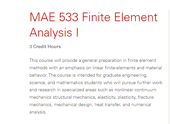
This course will provide a general preparation in finite element methods with an emphasis on linear finite-elements and material behavior. The course is intended for graduate engineering, science, and mathematics students who will pursue further work and research in specialized areas such as nonlinear continuum mechanics structural mechanics, elasticity, plasticity, fracture mechanics, mechanical design, heat transfer, and numerical analysis.
PREREQUISITES
Students will develop the mathematical and solid mechanics background to solve and analyze linear stress and analysis problems with the appropriate finite-element methodologies and numerical approximations. Applications of real-world problems with a focus on solid mechanics and elasticity. Course Requirements HOMEWORK: 6-8 assignments. EXAMINATIONS: Midterm and Final. SOFTWARE REQUIREMENTS: ANSYS will be used for different class projects. Other similar commercial FEM codes can be used. Knowledge of Fortran, C, C++, Matlab, or other programming languages will be useful Textbook Most of the material will be based on class notes and lectures. Students will be provided copies of the notes and the lectures.
MAE533 Finite Element Method HELP(EXAM HELP, ONLINE TUTOR)
问题 1.
Example 1.1 Equation of motion of a solid bar a) Derive the equation of motion of an elastic bar in terms of its deflection $u(x, t)$. Initially, assume that the bar has a variable cross-sectional area $A(x)$ and that it is subjected to distributed axial load $q(x, t)$ and a concentrated force $F$ at its free end as shown in Fig. 1.2. Also assume small deflections, linear elastic material behavior with constant elastic modulus $E$, and constant mass density $\rho$. b) Obtain the steady state solution for the case of constant cross-section and zero distributed force.
Solution 1.1a: The solution domain $\Omega$ for this problem spans $0<x<L$. The boundaries $\Gamma$ of the solution domain are located at $x=0$ and $x=L$. Internal forces develop in the bar in response to external loading. The internal normal force $N(x)$ at the cross-section $x$ can be defined as follows: $$ N(x)=\bar{\sigma}(x) A(x) $$ where the average normal stress $\bar{\sigma}$ is defined as follows: $$ \bar{\sigma}(x)=\frac{1}{A(x)} \int_{A(x)} \sigma d A $$ and where $\sigma$ is the internal normal stress, $A$ is the cross-sectional area of the bar. The equation of motion of the bar can be obtained by using Newton’s second law on a small segment of the bar (Fig. 1.2). The balance of internal and inertial forces gives, $$ \begin{aligned} & \sum F_x=\rho A d x \frac{\partial^2 u}{\partial t^2} \ & -N+q d x+\left(N+\frac{\partial N}{\partial x} d x\right)=\rho A d x \frac{\partial^2 u}{\partial t^2} \ & \frac{\partial N}{\partial x}=-q+\rho A \frac{\partial^2 u}{\partial t^2} \end{aligned}
Textbooks
• An Introduction to Stochastic Modeling, Fourth Edition by Pinsky and Karlin (freely available through the university library here) • Essentials of Stochastic Processes, Third Edition by Durrett (freely available through the university library here) To reiterate, the textbooks are freely available through the university library. Note that you must be connected to the university Wi-Fi or VPN to access the ebooks from the library links. Furthermore, the library links take some time to populate, so do not be alarmed if the webpage looks bare for a few seconds.
MAE533 Finite Element Method
Statistics-lab™可以为您提供engineeringonline.ncsu.edu MAE533 Finite Element Method有限元方法课程的代写代考和辅导服务! 请认准Statistics-lab™. Statistics-lab™为您的留学生涯保驾护航。
Choose one of the following functions to carry out the assignment:
$f(x)=\int_{0.1}^x e^{-t^2} d t$, where $0.1<x<5$
$f(x)=\int_{0.1}^x \sin (t) / t d t$, where $0.1<x<5$
$f(x)=\int_{0.1}^x e^{-t} \cos (t) d t$, where $0.1<x<5$
Write a python/matlab program and name it nInt.py or nInt.m.
The program nint will return the value of $f(x)$ when input a numerical value of $x$, where $0.1<$ $x<5$.
The program nInt will use a composite Simpson’s rule to calculate $f(x)$ with 1000 equally spaced partitions.
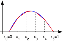
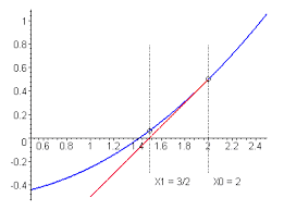
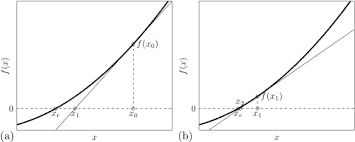
Show that there is at least one interception point for $f(x)$ and $y=1-x / 5$ in the interval $0.1<x<5$.
Find the interception point with either:
secant method; or
Newton’s method.
Plot $f(x), y=1-x / 5$ and the interception point on a same graph.
Comment on the accuracy of the interception point estimation, and how you will be able to improve the estimation.
I will choose the function $f(x)=\int_{0.1}^x e^{-t^2} dt$ for this assignment.
Python/Matlab code for nInt function:
pythonCopy codeimport numpy as np

def f(x):
    return np.exp(-0.01) + 2*np.sum(np.exp(-np.linspace(0.1, x, 1000)**2))

def nInt(x):
    h = (x - 0.1) / 1000
    integral = h / 3 * (f(0.1) + 4*f(np.linspace(0.1+h, x-h, 500)).sum() + 2*f(np.linspace(0.1+2*h, x-2*h, 499)).sum() + f(x))
    return integral
To show that there is at least one interception point for $f(x)$ and $y=1-x/5$ in the interval $0.1<x<5$, we can plot the two functions and observe their intersection:
The accuracy of the interception point estimation depends on the chosen tolerance and the method used. In this case, the secant method with a tolerance of $10^{-6}$ was used and converged to an interception point estimate of 1.0747. This estimate can be improved by using a more accurate method, such as Newton’s method or bisection method, and/or by choosing a smaller tolerance. Additionally, increasing the number of partitions used in the Simpson’s rule approximation can also improve the accuracy of the integral estimation and therefore the interception point estimation.
问题 2.
Consider a particle in two dimensions with Cartesian coordinates $x$ and $y$, and momentum $\left(p_x, p_y\right)$. The state of the system can be represented as a point $\left(x, y, p_x, p_y\right)$ in four-dimensional phase space. Suppose the particle has potential energy $V(x, y)$ and mass 1 . Then, its total energy is $$ H=\frac{1}{2}\left(p_x^2+p_y^2\right)+V(x, y), $$ and the equations of motion can be written as (Hamiltons equations) $$ \begin{array}{r} \frac{d x}{d t}=\frac{\partial H}{\partial p_x}=p_x \ \frac{d y}{d t}=\frac{\partial H}{\partial p_y}=p_y \ \frac{d p_x}{d t}=-\frac{\partial H}{\partial x}=-\frac{\partial V}{\partial x} \ \frac{d p_y}{d t}=-\frac{\partial H}{\partial y}=-\frac{\partial V}{\partial y} \end{array} $$ The solution to this system of equations, for given initial values $\left(x(0), y(0), p_x(0), p_y(0)\right)$, can be represented as a curve in phase space, $t \mapsto\left(x(t), y(t), p_x(t), p_y(t)\right)$. Along this curve the energy is conserved. Hence, the curve falls on a three-dimensional hypersurface $S_E$ corresponding to constant $H$, $$ S_E=\left{\left(x, y, p_x, p_y\right): H\left(x, y, p_x, p_y\right)=E=\text { constant }\right} $$ The following are some of the common potentials that used in modelling physical problems: \begin{tabular}{ll} \hline Hénon-Heiles Potential & $V=\frac{1}{2}\left(x^2+y^2\right)+x^2 y-\frac{1}{3} y^3$ \ Central Potential & $V=\left(x^2+y^2\right)^2$ \ \hline \end{tabular} Choose one of the above potential and answer the following questions:
Plot the equipotential curves for the potential. The equipotential curve is represented by the curve ${(x, y): V(x, y)=$ constant $}$, where along this curve the potential $V$ is constant.
For the Hénon-Heiles potential, plot the equipotential curves for $V=1 / 6,0.1,0.05$, and $0.01$.
For the Central potential, plot the equipotential curves for $V=1 / 6,0.1,0.05$, and $0.01$.
I choose the Hénon-Heiles potential $V=\frac{1}{2}\left(x^2+y^2\right)+x^2 y-\frac{1}{3} y^3$.
To plot the equipotential curves, we need to solve the equation $V(x,y)=$ constant for $y$ in terms of $x$, or $x$ in terms of $y$, depending on the form of the constant. Then we can plot the resulting curve for various values of the constant.
For $V=1/6$, we have \begin{align*} \frac{1}{2}\left(x^2+y^2\right)+x^2 y-\frac{1}{3} y^3 &= \frac{1}{6} \ y^3 + 3x^2 y – x^2 -\frac{1}{2}y^2 &= 0 \end{align*} We can plot this equation using matplotlib:
pythonCopy codeimport numpy as np
import matplotlib.pyplot as plt

# Constants
V = 1/6

# Create a grid of points to plot
x = np.linspace(-2, 2, 200)
y = np.linspace(-2, 2, 200)
X, Y = np.meshgrid(x, y)

# Calculate the equation
Z = Y**3 + 3*X**2*Y - X**2 - 0.5*Y**2 - V

# Plot the contour
plt.contour(X, Y, Z, levels=[0])
plt.axis('equal')
plt.title('Equipotential Curve for V=1/6')
plt.show()
This produces the following plot:
Similarly, we can plot the equipotential curves for $V=0.1,0.05,$ and $0.01$:
pythonCopy code# Constants
V = [0.1, 0.05, 0.01]

# Create a grid of points to plot
x = np.linspace(-2, 2, 200)
y = np.linspace(-2, 2, 200)
X, Y = np.meshgrid(x, y)

# Calculate and plot the contours
for v in V:
    Z = Y**3 + 3*X**2*Y - X**2 - 0.5*Y**2 - v
    plt.contour(X, Y, Z, levels=[0])

# Set the plot parameters
plt.axis('equal')
plt.title('Equipotential Curves for Hénon-Heiles Potential')
plt.legend(['V=0.1', 'V=0.05', 'V=0.01'])
plt.show()
This produces the following plot:
Now, we will plot the equipotential curves for the Central potential $V=\left(x^2+y^2\right)^2$:
pythonCopy code# Constants
V = [0.1, 0.05, 0.01]

# Create a grid of points to plot
x = np.linspace(-2, 2, 200)
y = np.linspace(-2, 2, 200)
X, Y = np.meshgrid(x, y)

# Calculate and plot the contours
for v in V:
    Z = X**2 + Y**2 - np.sqrt(v)
    plt.contour(X, Y, Z, levels=[0])

# Set the plot parameters
plt
Textbooks
• An Introduction to Stochastic Modeling, Fourth Edition by Pinsky and Karlin (freely available through the university library here) • Essentials of Stochastic Processes, Third Edition by Durrett (freely available through the university library here) To reiterate, the textbooks are freely available through the university library. Note that you must be connected to the university Wi-Fi or VPN to access the ebooks from the library links. Furthermore, the library links take some time to populate, so do not be alarmed if the webpage looks bare for a few seconds.
This course gives an introduction to commutative rings and their modules. We study concepts such as localization, decomposition of modules, chain conditions for rings and modules, and dimension theory. The course gives a relevant background for studies in algebraic geometry, but also relates the theory to problems in number theory.
PREREQUISITES
After completing the course you
know the definition of commutative rings, local rings, prime and maximal ideals, and modules over commutative rings
are familiar with the notions of noetherian and artinian rings and modules
know how to localize rings and modules, and are familiar with important applications of localization
know the Hilbert basis theorem and the Hilbert Nullstellensatz
are familiar with the concepts of support and associated primes
know the definition of an exact sequence of modules, and you also know important properties and applications of exact sequences
know the concept of direct limit and you can compute this limit in some non-trivial examples
know how to define tensor products of modules and are familiar with the concept of flatness
know Krull-Cohen-Seidenberg theory
know the basic results in the dimension theory for local rings
know how to complete a ring in an ideal.
MAT4200 Representation theory HELP(EXAM HELP, ONLINE TUTOR)
问题 1.
Problem 1: Given ideals $I, J$ of a ring $A$, we define $I J=\left{\sum_i a_i b_i \mid a_i \in I, b_i \in J\right}$. Show that (1) $\sqrt{I+J}=\sqrt{\sqrt{I}+\sqrt{J}}$. (2) $\sqrt{I J}=\sqrt{I} \cap \sqrt{J}$. (3) If $I$ is prime, then $\sqrt{I^n}=\sqrt{I}=I$ for all $n>0$.
(1) Firstly, we show that $\sqrt{I+J}\subseteq \sqrt{\sqrt{I}+\sqrt{J}}$. Suppose $x\in \sqrt{I+J}$, then there exists a positive integer $n$ such that $x^n\in I+J$. Write $x^n=\sum_i a_i+b_i$, where $a_i\in I$ and $b_i\in J$. Since $\sqrt{I}$ is an ideal, we have $(\sum_i a_i)^m\in I$ for some positive integer $m$, and similarly $(\sum_i b_i)^k\in J$ for some positive integer $k$. Then we have \begin{align*} x^n&=(\sum_i a_i+b_i)^n\ &=\sum_{i_1,i_2,\dots,i_n}\binom{n}{i_1,i_2,\dots,i_n}a_{i_1}a_{i_2}\dots a_{i_n}(\sum_i b_i)^{n-i_1-i_2-\dots-i_n}\ &\in I^n+J^n+\sum_{i=1}^{n-1}I^{i}J^{n-i}+\sum_{i=1}^{n-1}J^{i}I^{n-i}\ &\subseteq (I+\sqrt{I}J)^n+(J+\sqrt{J}I)^n\ &\subseteq (\sqrt{I}+\sqrt{J})^n \end{align*} where the first inclusion is due to the binomial expansion of $(\sum_i a_i+b_i)^n$ and the second inclusion is due to the fact that $I\subseteq \sqrt{I}$ and $J\subseteq \sqrt{J}$. Therefore, we have $x\in \sqrt{\sqrt{I}+\sqrt{J}}$.
Secondly, we show that $\sqrt{I+J}\supseteq \sqrt{\sqrt{I}+\sqrt{J}}$. Suppose $x\in \sqrt{\sqrt{I}+\sqrt{J}}$, then there exists a positive integer $n$ such that $x^n\in \sqrt{I}+\sqrt{J}$. Write $x^n=a+b$ where $a\in \sqrt{I}$ and $b\in \sqrt{J}$. Since $\sqrt{I}$ and $\sqrt{J}$ are ideals, we have $a^m\in I$ and $b^k\in J$ for some positive integers $m$ and $k$. Then we have \begin{align*} x^n&=(a+b)^n\ &=\sum_{i_1,i_2,\dots,i_n}\binom{n}{i_1,i_2,\dots,i_n}a^{i_1}b^{i_2}\dots a^{i_{n-1}}b^{i_n}\ &\in I^n+J^n+\sum_{i=1}^{n-1}I^{i-1}J^{n-i}a^i+\sum_{i=1}^{n-1}J^{i-1}I^{n-i}b^i\ &\subseteq (I+J)^n+\sum_{i=1}^{n-1}I^{i-1}J^{n-i}(I^m+J^k)+\sum_{i=1}^{n-1}J^{i-1}I^{n-i}(I^m+J^k)
问题 2.
Problem 2: Recall that $\operatorname{Spec} A$ denotes the set of all prime ideals of $A$. For every ideal $I \subset A$, we define $$ Z(I)={\mathfrak{p} \in \operatorname{Spec} A \mid I \subset \mathfrak{p}} $$ Show that (1) if $I \subset J$, then $Z(J) \subset Z(I)$. (2) $Z(\sqrt{I})=Z(I)$ (3) $Z(0)=\operatorname{Spec} A$ and $Z(A)=\varnothing$. (4) $\bigcap_{\alpha \in \mathcal{T}} Z\left(I_\alpha\right)=Z\left(\sum_{\alpha \in \mathcal{T}} I_\alpha\right)$ for any family of ideals $\left(I_\alpha\right)_{\alpha \in \mathcal{T}}$. (5) $Z(I) \cup Z(J)=Z(I \cap J)$ for any two ideals $I, J \subset A$. Hint: If $\mathfrak{p} \supset I \cap J \supset I J$, then $\mathfrak{p} \supset I$ or $\mathfrak{p} \supset J$ (explain this). The last three properties imply that the complements of $Z(I)$ form a topology on Spec $A$ (Zariski topology) so that $Z(I)$ are the closed subsets.
(1) Suppose $I \subset J$ and let $\mathfrak{p} \in Z(J)$, i.e., $J \subset \mathfrak{p}$. Since $I \subset J$, we have $I \subset \mathfrak{p}$, so $\mathfrak{p} \in Z(I)$. Thus, $Z(J) \subset Z(I)$.
(2) Let $\mathfrak{p} \in Z(\sqrt{I})$, i.e., $\sqrt{I} \subset \mathfrak{p}$. We want to show that $I \subset \mathfrak{p}$. Suppose not, then there exists $x \in I$ such that $x \notin \mathfrak{p}$. Since $\sqrt{I}$ is the intersection of all prime ideals containing $I$, it follows that $x^n \in \mathfrak{p}$ for some $n > 0$. But then $(x^n)^m \in \mathfrak{p}$ for all $m > 0$, so $x \in \sqrt{I} \subset \mathfrak{p}$, a contradiction. Thus, $I \subset \mathfrak{p}$ and hence $\mathfrak{p} \in Z(I)$. This shows that $Z(\sqrt{I}) \subset Z(I)$.
Conversely, suppose $\mathfrak{p} \in Z(I)$, i.e., $I \subset \mathfrak{p}$. Then $\sqrt{I} \subset \mathfrak{p}$ since $\mathfrak{p}$ is prime. Thus, $\mathfrak{p} \in Z(\sqrt{I})$. This shows that $Z(I) \subset Z(\sqrt{I})$. We have shown that $Z(\sqrt{I}) = Z(I)$.
(3) For any prime ideal $\mathfrak{p}$, we have $0 \subset \mathfrak{p}$, so $\mathfrak{p} \in Z(0)$. This shows that $Z(0) = \operatorname{Spec} A$.
On the other hand, if $A \subset \mathfrak{p}$ for some prime ideal $\mathfrak{p}$, then $1 \in A \subset \mathfrak{p}$, which implies that $\mathfrak{p} = A$. Thus, there are no prime ideals containing $A$, so $Z(A) = \varnothing$.
(4) Let $\mathfrak{p} \in \bigcap_{\alpha \in \mathcal{T}} Z(I_\alpha)$. Then $I_\alpha \subset \mathfrak{p}$ for all $\alpha$, so $\sum_{\alpha \in \mathcal{T}} I_\alpha \subset \mathfrak{p}$. This shows that $\mathfrak{p} \in Z\left(\sum_{\alpha \in \mathcal{T}} I_\alpha\right)$, so $\bigcap_{\alpha \in \mathcal{T}} Z(I_\alpha) \subset Z\left(\sum_{\alpha \in \mathcal{T}} I_\alpha\right)$.
• An Introduction to Stochastic Modeling, Fourth Edition by Pinsky and Karlin (freely available through the university library here) • Essentials of Stochastic Processes, Third Edition by Durrett (freely available through the university library here) To reiterate, the textbooks are freely available through the university library. Note that you must be connected to the university Wi-Fi or VPN to access the ebooks from the library links. Furthermore, the library links take some time to populate, so do not be alarmed if the webpage looks bare for a few seconds.
This course is an introduction to the representation theory of groups. Although the catalog title refers to finite groups, we will consider both finite and infinite groups. Representation theory studies the way in which a given group may act on vector spaces; in other words, it is concerned with representing groups as groups of matrices. We are mostly interested in irreducible representations, which are the building blocks for the construction of all representations of a given group. The main questions in representation theory are related to: (1) the construction of irreducible representations; (2) the calculation of certain algebraic invariants of these; (3) the decomposition of other representations into irreducibles.
Representation theory is a fundamental tool for studying group symmetry – geometric, analytic, or algebraic – by means of linear algebra. Its origins are mostly in the work of F. Frobenius, H. Weyl, I. Schur, and A. Young, about a century ago; Weyl’s work, for instance, is a milestone in the representation theory of Lie groups, which play a central role in many areas of mathematics. Important advances have been made during last century, through the study of representations of more and more general groups, and through a better understanding of the subtle combinatorics involved, which led to some very explicit constructions and computations. Today, representation theory plays an important role in many recent developments of mathematics and theoretical physics. A considerable amount of recent work is devoted to the representation theory of quantum groups, which are certain deformations of Lie groups, with applications to physics.
PREREQUISITES
Here are some pretty pictures that will come up in this course, created by John Stembridge; they illustrate the hyperplane arrangements corresponding to the root systems A3 and B3 .
Tentative syllabus: The main concepts of representation theory (characters, induced representations, irreducible representations). Symmetric functions (Young tableaux, Schur functions). Representations of the symmetric group (construction of the irreducible representations, Frobenius’s formula). Representations of the general linear group (Weyl’s construction, characters). Extension of Weyl’s construction to other Lie groups and Lie algebras. The main concepts of Lie theory and the classification of complex semisimple Lie algebras. Representations of complex simple Lie groups. The Weyl character formula. A hint about what lies ahead.
Prerequisites for this course are Math 220 (Linear Algebra) and Math 327 (Elementary Abstract Algebra). On the other hand, Math 420 (Abstract Algebra) and Math 424 (Advanced Linear Algebra) are helpful, but not required.
Math620 Representation theory HELP(EXAM HELP, ONLINE TUTOR)
问题 1.
(1) (5 pts) Let $G$ be a finite group. Show that the function
This sum is greater than or equal to zero and is zero if and only if $f(g)=0$ for all $g \in G$.
Therefore, $\langle f, f\rangle=0$ if and only if $f(g)=0$ for all $g \in G$, which implies that $\langle \cdot, \cdot\rangle$ is positive definite. Thus, $\langle \cdot, \cdot\rangle$ is an inner product on $\mathbb{C}[G]$.
问题 2.
(2) Instead of taking the trace of $\phi_g$ to define the character, one might try to do the same by taking the determinant of $\phi_g$ instead. This problem shows that this is not as useful since such a character would tell us nothing about non-abelian simple groups (and these are important).
For $\phi$ a representation of a finite group $G$, define a function
$$
\begin{aligned}
\operatorname{det} \phi: G & \longrightarrow \mathbb{C}^{\times} \
g & \longmapsto(\operatorname{det} \phi)(g)=\operatorname{det}\left(\phi_g\right)
\end{aligned}
$$
(a) (4 pts) Show det $\phi$ is a representatation (and hence it’s a character since characters are same as representations for one-dimensional representations).
(b) (5 pts) Show that if $G$ is a non-abelian simple group, then det $\phi$ is the trivial character.
Solution:
(a) Follows from the multiplicativity of the determinant.
(b) Since $\operatorname{det} \phi$ is a homomorphism, its kernel is a normal subgroup of $G$. Since $G$ is simple, it must be that $\operatorname{ker}(\operatorname{det} \phi)={e}$ or $\operatorname{ker}(\operatorname{det} \phi)=G$. If the former is true, then det $\phi$ is injective, and its image is a subgroup of $\mathbb{C}^{\times}$, which is abelian. This $G$ would be isomorphic to an abelian group, but this cannot by by assumption. So it must be that $\operatorname{ker}(\operatorname{det} \phi)=G$, in which case $\operatorname{det} \phi$ is the trivial homomorphism.
Here’s a more complete solution:
(b) Let $\phi$ be a representation of $G$, and let $\chi_{\operatorname{det} \phi}$ denote the character of the one-dimensional representation given by $\operatorname{det} \phi$. Suppose $G$ is non-abelian and simple. Then $\ker(\chi_{\operatorname{det} \phi})$ is a normal subgroup of $G$. Since $G$ is non-abelian and simple, the only normal subgroups of $G$ are the trivial subgroup ${e}$ and $G$ itself. If $\ker(\chi_{\operatorname{det} \phi}) = G$, then $\chi_{\operatorname{det} \phi}$ is the trivial character. Otherwise, $\ker(\chi_{\operatorname{det} \phi}) = {e}$, so $\chi_{\operatorname{det} \phi}$ is injective. But the image of $\chi_{\operatorname{det} \phi}$ is a subgroup of $\mathbb{C}^\times$, which is abelian. Thus $G$ would be isomorphic to an abelian group, which is a contradiction. Therefore, $\ker(\chi_{\operatorname{det} \phi}) = G$, so $\chi_{\operatorname{det} \phi}$ is the trivial character.
Textbooks
• An Introduction to Stochastic Modeling, Fourth Edition by Pinsky and Karlin (freely available through the university library here) • Essentials of Stochastic Processes, Third Edition by Durrett (freely available through the university library here) To reiterate, the textbooks are freely available through the university library. Note that you must be connected to the university Wi-Fi or VPN to access the ebooks from the library links. Furthermore, the library links take some time to populate, so do not be alarmed if the webpage looks bare for a few seconds.
statistics-lab™ 为您的留学生涯保驾护航 在代写有限元方法Finite Element Method方面已经树立了自己的口碑, 保证靠谱, 高质且原创的统计Statistics代写服务。我们的专家在代写有限元方法Finite Element Method代写方面经验极为丰富,各种代写有限元方法Finite Element Method相关的作业也就用不着说。
我们提供的有限元方法Finite Element Method及其相关学科的代写,服务范围广, 其中包括但不限于:
Statistical Inference 统计推断
Statistical Computing 统计计算
Advanced Probability Theory 高等概率论
Advanced Mathematical Statistics 高等数理统计学
(Generalized) Linear Models 广义线性模型
Statistical Machine Learning 统计机器学习
Longitudinal Data Analysis 纵向数据分析
Foundations of Data Science 数据科学基础
数学代写|有限元方法代写Finite Element Method代考|CIVL6840
数学代写|有限元方法代写Finite Element Method代考|Consistent nodal load vector
Equations $(6.37)(\mathrm{c}, \mathrm{d})$ are used to find statically equivalent forces and moments acting on the nodes due to distributed forces acting along the element. These nodal forces (and moments) are referred to as the consistent nodal forces (and moments). Consider the concentrated and the distributed forces acting on the element shown in Fig. 6.3. By using Eqs. (6.37) and (6.29) the following consistent nodal force vectors are found. Concentrated force: $-F_y \delta\left(x^{\prime}-a\right)$ acting along the $-y$-axis and located at $x^{\prime}=a$ $$ \left{r_q^{\prime}\right}^{(e)}=-F_y^{\prime}\left{\frac{b^2\left(L^{(e)}+2 a\right)}{L^{(e) 3}} \frac{a b^2}{L^{(e) 2}} \frac{a^2\left(L^{(e)}+2 b\right)}{L^{(e) 3}}-\frac{a^2 b}{L^{(e) 2}}\right}^T $$ where $b=L-a$. Linearly distributed force: $q_{y^{\prime}}=q_{y^{\prime} 1}+\frac{q_{y^{\prime} 2}-q_{y^{\prime} 1}}{L} x^{\prime}$. Note that $q_{y^{\prime}}$ is positive along the $+y^{\prime}$-axis. $$ \left{r_q^{\prime}\right}^{(e)}=\left{\frac{\left(7 q_{y_1}+3 q_{y_2}\right) L^{(c)}}{20} \frac{\left(3 q_{y_1}+2 q_{y_2}\right) L^{(e) 2}}{60} \frac{\left(3 q_{y 1}+7 q_{y_2}\right) L^{(e)}}{20}-\frac{\left(2 q_{y_1 1}+3 q_{y_2 2}\right) L^{(e) 2}}{60}\right}^T $$ Distributed force with constant magnitude: $q_{y^{\prime}}\left(x^{\prime}\right)=q_{y^{\prime} 0}$ which points along the $+y^{\prime}$-axis. $$ \left{r_q{ }^{\prime}\right}^{(e)}=\left{\frac{q_{y_0} L^{(e)}}{2} \frac{q_{y^{\prime} 0} L^{(e) 2}}{12} \frac{q_{y_0 0} L^{(e)}}{2}-\frac{q_{y_0 0} L^{(e) 2}}{12}\right}^T $$ The signs of the forces in these vectors are determined by the sign convention defined in Fig. 6.1.
数学代写|有限元方法代写Finite Element Method代考|General beam element with membrane
In many load bearing situations stretching and bending occurs on the same member, simultaneously (Fig. 6.4). The element stiffness matrix that represents the equilibrium of such a member is obtained by using the superposition of membrane and bending responses. Note that here we consider small deflection cases where these two effects can be assumed to be uncoupled from one another. The equilibrium equation for such a generic beam element is represented in matrix form as follows: $$ \left[k_{m b}^{\prime}\right]^{(e)}\left{d_{m b}\right}^{(e)}=\left{r_{m b}\right}^{(e)} $$ This relationship can be obtained by using a superposition of the membrane and beam mechanics, represented by Eqs. (5.22) and (6.38), $$ \left[k_m{ }^{\prime}\right]^{(e)}\left{d_m{ }^{\prime}\right}^{(e)}+\left[k_b^{\prime}\right]^{(e)}\left{d_b{ }^{\prime}\right}^{(e)}=\left{r_m{ }^{\prime}\right}^{(e)}+\left{r_b\right}^{(e)} $$ As the membrane and the bending actions are uncoupled (at least in this presentation) the following variables can be easily identified, $$ \left.\left[k_{m b}\right]^{\prime}\right]^{(e)}=\left[\begin{array}{cccccc} k_m & 0 & 0 & -k_m & 0 & 0 \ 0 & 12 k_b & 6 k_b L^{(e)} & 0 & -12 k_b & 6 k_b L^{(e)} \ 0 & 6 k_b L^{(e)} & 4 k_b L^{(e) 2} & 0 & -6 k_b L^{(e)} & 2 k_b L^{(e) 2} \ -k_m & 0 & 0 & k_m & 0 & 0 \ 0 & -12 k_b & -6 k_b L^{(e)} & 0 & 12 k_b & -6 k_b L^{(e)} \ 0 & 6 k_b L^{(e)} & 2 k_b L^{(e) 2} & 0 & -6 k_b L^{(e)} & 4 k_b L^{(e) 2} \end{array}\right] $$ with $k_m=\frac{E A}{L^{(e)}}$ and $k_b=\frac{E I}{\left.L^{(e)}\right)}$ $$ \begin{aligned} & \left{d_{m b}{ }^{\prime}\right}^{(e)}=\left{\begin{array}{llllll} u_1^{\prime} & v_1^{\prime} & \theta_1^{\prime} & u_2^{\prime} & v_2^{\prime} & \theta_2^{\prime} \end{array}\right}^T \ & \left{r_{m b}\right}^{\prime(e)}=\left[\begin{array}{llllll} F_{x^{\prime} 1} & F_{y^{\prime} 1} & M_1 & F_{x^{\prime} 2} & F_{y^{\prime} 2} & M_2 \end{array}\right}^T \end{aligned} $$
数学代写|有限元方法代写Finite Element Method代考|Consistent nodal load vector
方程式 $(6.37)(\mathrm{c}, \mathrm{d})$ 用于查找由于沿单元作用的分布力而作用在节点上的静态等效力和力矩。这些节点力 (和力矩) 被称为一致节点力 (和力矩) 。考虑作用在图 $6.3$ 中所示的单元上的集中力和分布力。通过使 用方程式。(6.37) 和 (6.29) 找到以下一致的节点力矢量。 集中力量: $-F_y \delta\left(x^{\prime}-a\right)$ 沿着 $-y$-轴并位于 $x^{\prime}=a$ left{ $_r_{-} q^{\wedge}{$ prime $\left.} \backslash r i g h t\right}^{\wedge}{(e)}=-F _y^{\wedge}{\backslash$ prime $} \backslash l e f t\left{\backslash f r a c\left{b^{\wedge} 2 \backslash l e f t\left(L^{\wedge}{(e)}+2\right.\right.\right.$ a right $\left.)\right}{L \wedge{(e) 3}} \backslash f r a c\left{a b^{\wedge} 2\right}\left{L^{\wedge}{(e) 2\right.$ 在哪里 $b=L-a$. 线性分布力: $q_{y^{\prime}}=q_{y^{\prime} 1}+\frac{q_{y^{\prime} 2}-q_{y^{\prime}}}{L} x^{\prime}$. 注意 $q_{y^{\prime}}$ 沿为正 $+y^{\prime}$-轴。 Veft $\left{r_{-} q^{\wedge}{\backslash\right.$ prime $\left.} \backslash r i g h t\right} \wedge{(e)}=\backslash \operatorname{eft}\left{\backslash f r a c\left{\backslash \operatorname{lft}\left(7 q_{-}\left{y_{-} 1\right}+3 q_{_}\left{y_{-} 2\right} \backslash r i g h t\right) L^{\wedge}{(c)}\right}{20} \backslash f r a c\left{\backslash e f t\left(3 q_{-}\left{y_{-} 1\right}+2 q_{-}\left{y_{-}\right.\right.\right.\right.$ 大小恒定的分布力: $q_{y^{\prime}}\left(x^{\prime}\right)=q_{y^{\prime} 0}$ 哪个点沿着 $+y^{\prime}$-轴。 Veft{r_q {}$^{\wedge}{\backslash$ prime $\left.} \backslash r i g h t\right}^{\wedge}{(e)}=\bigvee$ left $\left{\right.$ frac $\left{q_{-}\left{y_{-} 0\right} L^{\wedge}{(e)}\right}{2} \backslash$ frac $\left{q_{_}\left{y^{\wedge}{\backslash p r i m e} 0\right} L^{\wedge}{(e) 2}\right}{12} \backslash f r a c\left{q_{-}\left{y_{-} 00\right.\right.$ 这些矢量中力的符号由图 $6.1$ 中定义的符号约定确定。
数学代写|有限元方法代写Finite Element Method代考|General beam element with membrane
statistics-lab™ 为您的留学生涯保驾护航 在代写有限元方法Finite Element Method方面已经树立了自己的口碑, 保证靠谱, 高质且原创的统计Statistics代写服务。我们的专家在代写有限元方法Finite Element Method代写方面经验极为丰富,各种代写有限元方法Finite Element Method相关的作业也就用不着说。
我们提供的有限元方法Finite Element Method及其相关学科的代写,服务范围广, 其中包括但不限于:
Statistical Inference 统计推断
Statistical Computing 统计计算
Advanced Probability Theory 高等概率论
Advanced Mathematical Statistics 高等数理统计学
(Generalized) Linear Models 广义线性模型
Statistical Machine Learning 统计机器学习
Longitudinal Data Analysis 纵向数据分析
Foundations of Data Science 数据科学基础
数学代写|有限元方法代写Finite Element Method代考|ENGR7961
数学代写|有限元方法代写Finite Element Method代考|Total potential energy of a beam element
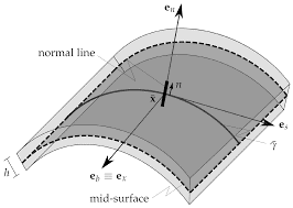
Similar to the development presented for the axial bar in Section 5.2.4, the total potential energy of the beam under the effect of external forces is expressed as follows: $$ \begin{aligned} & \pi_p^{(e)}=U^{(e)}-W^{(e)} \ & \pi_p^{(e)}=\int_A \int_0^{L^{(e)}} \sigma^{\prime} d \varepsilon^{\prime} d A d x^{\prime}-\left(\int_0^{L^{(-)}} v^{\prime}\left(F_b A+q\right) d x^{\prime}+v_1^{\prime} F_{y 1}{ }^{\prime}+v_2^{\prime} F_{y 2}{ }^{\prime}+\theta_1 M_1+\theta_2 M_2\right) \end{aligned} $$ where the first term represents the strain energy stored in the beam, and the second term represents the work done by the external forces. Note that for a beam we have $d A=b d y^{\prime}$ where $b$ is the breadth of the beam’s cross-section. The bending strain, is a longitudinal strain $\varepsilon_{x^{\prime}}$, which depends on the normal distance as measured from the neutral axis of the beam (Fig. 6.2) as given in Eq. (2.138), $$ \varepsilon_{x^{\prime}}=-y^{\prime} \frac{d^2 v^{\prime}}{d x^{\prime 2}} $$
The strain energy component of the total potential energy then becomes, $$ U_b^{(e)}=\frac{1}{2} \int_0^{L^{(e)}}\left[\int_A E\left(-y^{\prime} \frac{d^2 v^{\prime}}{d x^2}\right)^2 b d y^{\prime}\right] d x^{\prime}=\frac{1}{2} \int_0^{L^{(e)}} E\left(\frac{d^2 v^{\prime}}{d x^2}\right)^2\left(\int_{-c / 2}^{c / 2} y^2 b d y^{\prime}\right) d x^{\prime} $$ Note that the inner integral over the area represents the definition of the second moment of area $$ I=\int_{-c / 2}^{c / 2} y^{\prime 2} b d y^{\prime} $$ The strain energy due to bending $U_b^{(e)}$ in a beam element is therefore expressed as follows: $$ U_b^{(e)}=\frac{1}{2} \int_0^{L^{(e)}} E I\left(\frac{d^2 v^{\prime}}{d x^{\prime 2}}\right)^2 d x^{\prime}, \text { or } U_b^{(e)}=\frac{1}{2} \int_0^{L^{(e)}} E I\left(\frac{d \theta}{d x^{\prime}}\right)^2 d x^{\prime} $$
数学代写|有限元方法代写Finite Element Method代考|Finite element form of the equilibrium equations
The principle of minimum total potential energy states that the equilibrium conditions are found when the variation of the total potential energy functional is zero. For an Euler-Bernoulli beam element, this is expressed as follows: $$ \delta \pi_p^{(\varepsilon)}=\int_0^{L^{(c)}} E I \frac{d \theta}{d x^{\prime}} \frac{d \delta \theta}{d x^{\prime}} d x^{\prime}-\left(\int_0^{L^{(c)}} \delta v^{\prime}\left(F_{B y^{\prime}} A+q_y\right) d x^{\prime}+\delta v_1{ }^{\prime} F_{y_1}+\delta v_2{ }^{\prime} F_{y^{\prime}}+\delta \theta_1 M_1+\delta \theta_2 M_2\right) $$
In order to find an expression for the curvature, $d \theta / d x^{\prime}$ recall that the beam deflection $v^{\prime}$ is approximated as follows: $$ \begin{aligned} v^{\prime}\left(x^{\prime}\right) & =N_1^{(b)} v_1^{\prime}+N_2^{(b)} \theta_1+N_3^{(b)} v_2{ }^{\prime}+N_4^{(b)} \theta_2 \text { (a) } \ & =\left[N^{(b)}\right]\left{d_b^{\prime}\right}^{(e)} \end{aligned} $$ where $\left[N^{(b)}\right]$ and $\left{d_b^{\prime}\right}^{(e)}$ are the shape function matrix and the degree of freedom vector, (Eq. (6.10)(a)) respectively, $$ \left[\begin{array}{llll} N^{(b)} \end{array}\right]=\left[\begin{array}{llll} N_1^{(b)} & N_2^{(b)} & N_3^{(b)} & N_4^{(b)} \end{array}\right] $$ $N_i^{(L)}$ are the $\mathrm{C}^1$-continuous shape functions given by Eq. (6.5). Using this approximation, the curvature vector is found as follows: $$ \frac{d \theta}{d x^{\prime}}=\frac{d^2 v^{\prime}}{d x^{\prime 2}}=\frac{d^2}{d x^{\prime 2}}\left(\left[N^{(b)}\right]\left{d_b^{\prime}\right}^{(e)}\right)=\left[B^{(b)}\right]\left{d_b^{\prime}\right}^{(e)} $$ where $\left[\begin{array}{llll}B^{(b)}\end{array}\right]=\left[\begin{array}{llll}B_1^{(b)} & B_2^{(b)} & B_3^{(b)} & B_4^{(b)}\end{array}\right]$ is the curvature-displacement matrix with, $$ \begin{aligned} & B_1^{(b)}=\frac{d^2 N_1^{(b)}}{d x^2}=\left(-\frac{6}{L^{(e) 2}}+\frac{12 x^{\prime}}{L^{(e) 3}}\right), \quad B_2^{(b)}=\frac{d^2 N_2^{(b)}}{d x^{\prime 2}}=\left(-\frac{4}{L^{(e)}}+\frac{6 x}{L^{(e) 2}}\right), \ & B_3^{(b)}=\frac{d^2 N_3^{(b)}}{d x^{\prime 2}}=\left(\frac{6}{L^{(e) 2}}-\frac{12 x^{\prime}}{L^{(e) 3}}\right), \quad B_4=\frac{d^2 N_4^{(b)}}{d x^{\prime 2}}=\left(-\frac{2}{L^{(e)}}+\frac{6 x^{\prime}}{L^{(e) 2}}\right) \end{aligned} $$
数学代写|数值分析代写numerical analysis代考|Use of Automatic Differentiation
Automatic differentiation is such a wonderful technique, there is tendency to apply it indiscriminately. Some recent work, such as [131], can seem to promote this point of view. However, automatic differentiation is not infallible. To illustrate this, consider using the bisection method to solve $f(x, p)=0$ for $x$ : the solution $x$ is implicitly a function of $p: x=x(p)$. Provided for $p \approx p_0$ we have $f(a, p)<0$ and $f(b, p)>0$ for given fixed numbers $a<b$, bisection will give the solution $x(p)$ for $p \approx p_0$. However, in the bisection algorithm (Algorithm 40), we first look at $c=(a+b) / 2$ and evaluate $f(c, p)$ and use the sign of this function value to determine how to update the endpoints $a$ and $b$. Since $a$ and $b$ are constant, $\partial a / \partial p=\partial a / \partial p=0$, and so $\partial c / \partial p=0$. Continuing through the bisection algorithm we find that the solution returned has $\partial x^* / \partial p=0$. Which is wrong. From the Implicit Function Theorem we have $$ \begin{aligned} 0 & =\frac{\partial f}{\partial x}(x, p) \frac{\partial x}{\partial p}+\frac{\partial f}{\partial p}(x, p), \ \frac{\partial x}{\partial p} & =-\left(\frac{\partial f}{\partial p}(x, p)\right) /\left(\frac{\partial f}{\partial x}(x, p)\right) \end{aligned} $$ Once the solution $x(p)$ is found, we can find the derivatives $\partial f / \partial p$ and $\partial f / \partial x$ using automatic differentiation. We can then compute $\partial x / \partial p$ using the above formula, regardless of how $x(p)$ is computed. In a multivariate setting, the computation of derivatives of the solution $\boldsymbol{x}(\boldsymbol{p})$ of equations $\boldsymbol{f}(\boldsymbol{x}, \boldsymbol{p})=\mathbf{0}$ with respect to a parameter $p$ will involve solving a linear system of equations: $\nabla_p \boldsymbol{x}(\boldsymbol{p})=$ $-\nabla_x f(x, p)^{-1} \nabla_p f(x, p)$
Automatic differentiation is also heavily used in machine learning and neural networks. The main neural network training algorithm backpropagation is essentially an application of the main ideas of automatic differentiation [18] combined with a version of gradient descent.
If gradients $\nabla f(\boldsymbol{x})$ can be computed in $\mathcal{O}(\operatorname{oper}(f(\boldsymbol{x})))$ operations, what about second derivatives? Can we compute Hess $f(\boldsymbol{x})$ in $\mathcal{O}(\operatorname{oper}(f(\boldsymbol{x})))$ operations? The answer is no. Take, for example, the function $f(\boldsymbol{x})=\left(\boldsymbol{x}^T \boldsymbol{x}\right)^2$. The computation of $f(\boldsymbol{x})$ only requires oper $(f(\boldsymbol{x}))=2 n+1$ arithmetic operations. Then $$ \begin{aligned} \nabla f(\boldsymbol{x}) & =4\left(\boldsymbol{x}^T \boldsymbol{x}\right) \boldsymbol{x}, \ \text { Hess } f(\boldsymbol{x}) & =4\left(\boldsymbol{x}^T \boldsymbol{x}\right) I+8 \boldsymbol{x} \boldsymbol{x}^T . \end{aligned} $$ For general $\boldsymbol{x}$, Hess $f(x)$ has $n^2$ non-zero entries $\left(\frac{1}{2} n(n+1)\right.$ independent entries), so we cannot expect to “compute” Hess $f(\boldsymbol{x})$ in $\mathcal{O}(n)$ operations. However, we can compute $$ \text { Hess } \begin{aligned} f(\boldsymbol{x}) \boldsymbol{d} & =\left[4\left(\boldsymbol{x}^T \boldsymbol{x}\right) I+8 \boldsymbol{x} \boldsymbol{x}^T\right] \boldsymbol{d} \ & =4\left(\boldsymbol{x}^T \boldsymbol{x}\right) \boldsymbol{d}+8 \boldsymbol{x}\left(\boldsymbol{x}^T \boldsymbol{d}\right) \end{aligned} $$ in just $7 n+2=\mathcal{O}(n)$ arithmetic operations. In general, we can compute Hess $f(\boldsymbol{x}) \boldsymbol{d}$ in $\mathcal{O}(\operatorname{oper}(f(\boldsymbol{x})))$. We can do this by applying the forward mode to compute $$ \left.\frac{d}{d s} \nabla f(\boldsymbol{x}+s \boldsymbol{d})\right|_{s=0}=\text { Hess } f(\boldsymbol{x}) \boldsymbol{d} $$ where we use the reverse mode for computing $\nabla f(z)$.
数学代写|数值分析代写numerical analysis代考|Basic Theory
We start with an equivalent expression of the initial value problem (6.1.1): $$ \boldsymbol{x}(t)=\boldsymbol{x}0+\int{t_0}^t \boldsymbol{f}(s, \boldsymbol{x}(s)) d s \quad \text { for all } t . $$ Peano proved the existence and uniqueness of solutions to the initial value problem using a fixed point iteration [200] named in his honor: (6.1.3) $\quad \boldsymbol{x}{k+1}(t)=\boldsymbol{x}_0+\int{t_0}^t \boldsymbol{f}\left(s, \boldsymbol{x}_k(s)\right) d s \quad$ for all $t$ for $k=0,1,2, \ldots$, with $\boldsymbol{x}_0(t)=\boldsymbol{x}_0$ for all $t$. To show that the iteration (6.1.3) is well defined and converges, we need to make some assumptions about the right-hand side function $f$. Most specifically we assume that $\boldsymbol{f}(t, \boldsymbol{x})$ is continuous in $(t, \boldsymbol{x})$ and Lipschitz continuous in $\boldsymbol{x}$ : there must be a constant $L$ where (6.1.4) $|\boldsymbol{f}(t, \boldsymbol{u})-\boldsymbol{f}(t, \boldsymbol{v})| \leq L|\boldsymbol{u}-\boldsymbol{v}| \quad$ for all $t, \boldsymbol{u}$, and $\boldsymbol{v}$. Caratheodory extended Peano’s existence theorem to allow for $\boldsymbol{f}(t, x)$ continuous in $\boldsymbol{x}$ and measurable in $t$ with a bound $|\boldsymbol{f}(t, \boldsymbol{x})| \leq m(t) \varphi(|\boldsymbol{x}|)$ with $m(t) \geq 0$ integrable in $t$ over $\left[t_0, T\right], \varphi$ continuous, and $\int_1^{\infty} d r / \varphi(r)=\infty$. Uniqueness holds if the Lipschitz continuity condition (6.1.4) holds with an integrable function $L(t)$ : (6.1.5) $|\boldsymbol{f}(t, \boldsymbol{u})-\boldsymbol{f}(t, \boldsymbol{v})| \leq L(t)|\boldsymbol{u}-\boldsymbol{v}| \quad$ for all $t, \boldsymbol{u}, \boldsymbol{v}$. We will focus on the case where $\boldsymbol{f}(t, \boldsymbol{x})$ is continuous in $t$ and Lipschitz in $\boldsymbol{x}$ (6.1.4) since numerical estimation of integrals of general measurable functions is essentially impossible.
Theorem 6.1 Suppose $\boldsymbol{f}: \mathbb{R} \times \mathbb{R}^n \rightarrow \mathbb{R}^n$ is continuous and (6.1.4) holds. Then the initial value problem (6.1.1) has a unique solution $\boldsymbol{x}(\cdot)$.
Proof We use the Peano iteration (6.1.3) to show the solution to the integral form (6.1.2) of (6.1.1) has a unique solution. To do that we show that the iteration (6.1.3) is a contraction mapping (Theorem 3.3) on the space of continuous functions $\left[t_0, t_0+\delta\right] \rightarrow \mathbb{R}^n$ for $\delta=1 /(2 L)$. This establishes the existence and uniqueness of the solution $x:\left[t_0, t_0+\delta\right] \rightarrow \mathbb{R}^n$. To show existence and uniqueness beyond this, let $t_1=t_0+\delta$ and $\boldsymbol{x}_1=\boldsymbol{x}\left(t_0+\delta\right)$.
Forward mode is the simplest approach for automatic differentiation, both conceptually and in practice. This idea is sometimes implemented as dual numbers in programming languages that allow overloaded arithmetic operations and functions. A dual number is a pair $x=(x . v, x . d)$ where $x . v$ represents the value of the number, and $x . d$ its derivative with respect to some single parameter, say $d x / d s$. Ordinary numbers are treated as constants, and so are represented as $(v, 0)$ where $v$ is the number. Operations on dual numbers $x$ and $y$ can be described as $$ \begin{aligned} x+y & =(x \cdot v+y \cdot v, x \cdot d+y \cdot d) \ x-y & =(x \cdot v-y \cdot v, x \cdot d-y \cdot d) \ x \cdot y & =(x \cdot v \cdot y \cdot v, x \cdot v \cdot y \cdot d+x \cdot d \cdot y \cdot v) \ x / y & =\left(x \cdot v / y \cdot v,(x \cdot d \cdot y \cdot v-x \cdot v \cdot y \cdot d) /(y \cdot v)^2\right) \ f(x) & =\left(f(x \cdot v), f^{\prime}(x \cdot v) \cdot x \cdot d\right) \end{aligned} $$ This can be extended to handle higher order derivatives, such as triple numbers $x=$ $(x . v, x . d, x . c)$ where $x . d=d x / d s$ and $x . c=d^2 x / d s^2$. Then for triple numbers, for example, the arithmetic rules include $$ \begin{aligned} & x \cdot y=(x \cdot v \cdot y \cdot v, x \cdot v \cdot y \cdot d+x \cdot d \cdot y \cdot v, x \cdot v \cdot y \cdot c+2 x \cdot d \cdot y \cdot d+x \cdot c \cdot y \cdot v) \ & f(x)=\left(f(x \cdot v), f^{\prime}(x \cdot v) \cdot x \cdot d, f^{\prime}(x \cdot v) x \cdot c+f^{\prime \prime}(x \cdot v)(x \cdot d)^2\right) \end{aligned} $$ The derivatives computed would be exact if the underlying arithmetic were exact. Thus the only errors in the computed derivatives are due to roundoff error. This does not guarantee accurate results, but they rarely fail.
Forward mode automatic differentiation is suitable where there is one, or a small number, of independent variables with respect to which we wish to computed derivatives. If we wish to compute gradients for many inputs, we need a different method.
数学代写|数值分析代写numerical analysis代考|Reverse Mode
The reverse mode of automatic differentiation is best suited to compute gradients of a single output function with respect to many inputs. The basic idea has been rediscovered multiple times that we know of, but the modern approach can be traced back at least to Seppo Linnainmaa in his PhD thesis that was later published [163]. For this, we need to conceptually flatten the execution of a piece of code so that it is written as a “straight-line code” with branches and loops removed. For example, the loop should be written as it is executed: $$ \begin{aligned} & x_1 \leftarrow f\left(x_0\right) \ & x_2 \leftarrow f\left(x_1\right) \ & x_3 \leftarrow f\left(x_2\right) \ & x_4 \leftarrow f\left(x_3\right) \end{aligned} $$ The index $j$ in $x_j$ indicates a potentially new value for the variable ” $x$ ” for each pass through the body of the loop.
In reverse mode automatic differentiation, this execution path and the values of variables along this path must be saved, at least at strategically important points of the execution of the original code. This can be represented in a computational graph of the execution of the code. Note that in the computational graph, each variable must only be assigned a value once. If a value of a variable is over-written, then we create a new variable for the computational graph, as shown in the example of the loop above. The code $$ \begin{aligned} & u \leftarrow r \cdot s \ & v \leftarrow r^s \ & x \leftarrow \varphi(u, v) \ & y \leftarrow x \cdot r \end{aligned} $$ can be represented by the computational graph in Figure 5.5.2. We compute the partial derivatives $\partial y / \partial z$ for $z$ each of the variables in the computational graph as we go back through the computational graph.
前向模式是最简单的自动微分方法,无论是在概念上还是在实践中。这个想法有时在允许重载算术运算和 函数的编程语言中实现为双数。双数是一对 $x=(x . v, x . d)$ 在哪里 $x . v$ 表示数字的值,并且 $x . d$ 它关于 某个单一参数的导数,比如说 $d x / d s$. 普通数被视为常数,因此表示为 $(v, 0)$ 在哪里 $v$ 是数字。 双数运算 $x$ 和 $y$ 可以描述为 $$ x+y=(x \cdot v+y \cdot v, x \cdot d+y \cdot d) x-y \quad=(x \cdot v-y \cdot v, x \cdot d-y \cdot d) x \cdot y=(x \cdot v \cdot y \cdot v $$ 这可以扩展到处理高阶导数,例如三重数 $x=(x . v, x . d, x . c)$ 在哪里 $x . d=d x / d s$ 和 $x . c=d^2 x / d s^2$. 那么对于三重数,例如,算术规则包括 $$ x \cdot y=(x \cdot v \cdot y \cdot v, x \cdot v \cdot y \cdot d+x \cdot d \cdot y \cdot v, x \cdot v \cdot y \cdot c+2 x \cdot d \cdot y \cdot d+x \cdot c \cdot y \cdot v) \quad f(x) $$ 如果基础算法是精确的,则计算出的导数将是精确的。因此,计算出的导数中唯一的误差是由于舍入误差 造成的。这并不能保证准确的结果,但它们很少会失败。 正向模式自动微分适用于我们希望计算导数的一个或少量自变量的情况。如果我们㹷望为许多输入计算梯 度,我们需要一种不同的方法。
数学代写|数值分析代写numerical analysis代考|Reverse Mode
自动微分的反向模式最适合计算单个输出函数相对于多个输入的梯度。据我们所知,基本思想已被多次重 新发现,但现代方法至少可以追溯到 Seppo Linnainmaa 在其后来发表的博士论文中 [163]。为此,我们 需要在概念上将一段代码的执行扁平化,使其写成去除了分支和循环的“直线代码”。例如,循环 应该在执行时写成: $$ x_1 \leftarrow f\left(x_0\right) \quad x_2 \leftarrow f\left(x_1\right) x_3 \leftarrow f\left(x_2\right) \quad x_4 \leftarrow f\left(x_3\right) $$ 指标 $j$ 在 $x_j$ 指示变量的潜在新值” $x$ ” 每次通过循环体。 在逆向模式自动微分中,这条执行路径和沿着这条路径的变量值必须被保存,至少在原始代码执行的战略 要点。这可以在代码执行的计算图中表示。请注意,在计算图中,每个变量只能被赋值一次。如果变量的 值被覆盖,那么我们为计算图创建一个新变量,如上面的循环示例所示。 代码 $$ u \leftarrow r \cdot s \quad v \leftarrow r^s x \leftarrow \varphi(u, v) \quad y \leftarrow x \cdot r $$ 可以用图 5.5.2 中的计算图来表示。 我们计算偏导数 $\partial y / \partial z$ 为了 $z$ 当我们返回计算图时,计算图中的每个变量。
数学代写|交换代数代写commutative algebra代考|Definition, Changing Generator Set
A finitely presented module is an $\mathbf{A}$-module $M$ given by a finite number of generators and relations. Therefore it is a module with a finite generator set having a finitely generated syzygy module. Equivalently, it is a module $M$ isomorphic to the cokernel of a linear map $$ \gamma: \mathbf{A}^m \longrightarrow \mathbf{A}^q $$ The matrix $G \in \mathbf{A}^{q \times m}$ of $\gamma$ has as its columns a generator set of the syzygy module between the generators $g_i$ which are the images of the canonical base of $\mathbf{A}^q$ by the surjection $\pi: \mathbf{A}^q \rightarrow M$. Such a matrix is called a presentation matrix of the module $M$ for the generator set $\left(g_1, \ldots, g_q\right)$. This translates into
$\left[g_1 \cdots g_q\right] G=0$, and
every syzygy between the $g_i$ ‘s is a linear combination of the columns of $G$, i.e.: if $\left[g_1 \cdots g_q\right] C=0$ with $C \in \mathbf{A}^{q \times 1}$, there exists a $C^{\prime} \in \mathbf{A}^{m \times 1}$ such that $C=G C^{\prime}$.
1) A free module of rank $k$ is a finitely presented module presented by a matrix column formed of $k$ zeros. ${ }^1$ More generally every simple matrix is the presentation matrix of a free module of finite rank. 2) Recall that a finitely generated projective module is a module $\boldsymbol{P}$ isomorphic to the image of a projection matrix $F \in \mathbb{M}_n$ (A) for a specific integer $n$. Since $\mathbf{A}^n=\operatorname{Im}(F) \oplus \operatorname{Im}\left(\mathrm{I}_n-F\right)$, we obtain $P \simeq \operatorname{Coker}\left(\mathrm{I}_n-F\right)$. This shows that every finitely generated projective module is finitely presented. 3) Let $\varphi: V \rightarrow V$ be an endomorphism of a finite-dimensional vector space over a discrete field $\mathbf{K}$. Consider $V$ as a $\mathbf{K}[X]$-module with the following external law $$ \begin{cases}\mathbf{K}[X] \times V & \rightarrow V \ (P, u) & \mapsto P \cdot u:=P(\varphi)(u)\end{cases} $$ Let $\left(u_1, \ldots, u_n\right)$ be a basis of $V$ as a $\mathbf{K}$-vector space and $A$ be the matrix of $\varphi$ with respect to this basis. Then we can show that a presentation matrix of $V$ as a $\mathbf{K}[X]$-module for the generator set $\left(u_1, \ldots, u_n\right)$ is the matrix $X \mathrm{I}_n-A$ (see Exercise 3). 1.0 Lemma When we change a finite generator set for a given finitely presented module, the syzygies between the new generators form a finitely generated module again.
Consider a ring $\mathbf{A}$ and a generator set $\left(a_1, \ldots, a_n\right)=(a)$ for a finitely generated ideal $\mathfrak{a}$ of $\mathbf{A}$. We are interested in the $\mathbf{A}$-module structure of $\boldsymbol{a}$.
Among the syzygies between the $a_i$ ‘s there are what we call the trivial syzygies (or trivial relators if we see them as algebraic dependence relations over $\mathbf{k}$ when $\mathbf{A}$ is a k-algebra): $$ a_i a_j-a_j a_i=0 \text { for } i \neq j . $$ If $\mathfrak{a}$ is finitely presented, we can always take a presentation matrix of $\mathfrak{a}$ for the generator set $(a)$ in the form $$ W=\left[R_{a} \mid U\right], $$ where $R_{a}$ is “the” $n \times n(n-1) / 2$ matrix of trivial syzygies (the order of the columns is without importance). For example, for $n=4$ $$ R_{a}=\left[\begin{array}{cccccc} a_2 & a_3 & 0 & a_4 & 0 & 0 \ -a_1 & 0 & a_3 & 0 & a_4 & 0 \ 0 & -a_1 & -a_2 & 0 & 0 & a_4 \ 0 & 0 & 0 & -a_1 & -a_2 & -a_3 \end{array}\right] . $$ 2.1 Lemma (Determinantal ideals of the matrix of trivial syzygies) Using the above notations, we have the following results.
$\mathcal{D}n\left(R{a}\right)={0}$.
If $1 \leqslant r<n$, then $\mathcal{D}r\left(R{a}\right)=\mathfrak{a}^r$ and $$ \mathfrak{a}^r+\mathcal{D}r(U) \subseteq \mathcal{D}_r(W) \subseteq \mathfrak{a}+\mathcal{D}_r(U) . $$ In particular, we have the equivalence $$ 1 \in \mathcal{D}{\mathbf{A}, r}(W) \Longleftrightarrow 1 \in \mathcal{D}_{\mathbf{A} / \mathfrak{a}, r}(\bar{U}) \text { where } \bar{U}=U \bmod \mathfrak{a} . $$
考虑一枚戒指 $\mathbf{A}$ 和发电机组 $\$ \backslash e f t\left(a_{-} 1, V\right.$ dots, a_n $\backslash$ right $)=($ a $)$ fora finitelygeneratedideal \mathfrak{a}of $\backslash$ mathbf{A}. Weareinterestedinthe $\backslash$ mathbf ${\mathrm{A}}-$ modulestructureof Vboldsymbol{a}\$。 在 syzygies 之间 $a_i$ 有什么我们称之为平凡的 syzygies(或者平凡的相关关系,如果我们将它们视为代数 依赖关系 $\mathbf{k}$ 什么时候 $\mathbf{A}$ 是一个 $k-$ 代数): $$ a_i a_j-a_j a_i=0 \text { for } i \neq j . $$ 如果 $\mathfrak{a}$ 是有限呈现的,我们总是可以采用表示矩阵 $\mathfrak{a}$ 对于发电机组 $\$(a)$ inthe form $\$$ $W=\backslash l e f t\left[R _{a} \backslash m i d\right.$ U\right } ] \text { , } $\$ \$$ 其中 $\$ R_{-}{a} i s$ “the” $n$ Itimes $n(\mathrm{n}-1) / 2$ matrixoftrivialsyzygies(theorderofthecolumnsiswithoutimportance). Forexample, for $\mathrm{n}=4 \$$ $R _{a}=\backslash \operatorname{left}[$ 正确的]。 $\$ \$$ $2.1$ 引理 (平凡合集矩阵的行列式理想) 使用上述符号,我们得到以下结果。
$\$ \backslash$ mathcal${D} n \backslash e f t(R{a} \backslash r i g h t)={0} \$$ 。
如果 $1 \leqslant r<n$, 那么 $\$ \backslash m a t h c a l{D} r \backslash l e f t(R{a} \backslash r i g h t)=\backslash m a t h f r a k{a} \wedge$ rand $\mathfrak{a}^r+\mathcal{D} r(U) \subseteq \mathcal{D}r(W) \subseteq \mathfrak{a}+\mathcal{D}_r(U)$.Inparticular, wehavetheequivalence $1 \in \mathcal{D} \mathbf{A}, r(W) \Longleftrightarrow 1 \in \mathcal{D}{\mathbf{A} / \mathfrak{a}, r}(\bar{U})$ where $\bar{U}=U \bmod a . \$$ $$ \text { 3. } \mathcal{D}_n(W)=\mathcal{D}_n(U) $$
We now move onto a formal Nullstellensatz, formal in the sense that it applies (in classical mathematics) to an arbitrary ideal over an arbitrary ring. Nevertheless to have a constructive statement we will be content with a polynomial ring $\mathbb{Z}[X]$ for our arbitrary ring and a finitely generated ideal for our arbitrary ideal.
Although this may seem very restrictive, practice shows that this is not the case because we can (almost) always apply the method of undetermined coefficients to a commutative algebra problem; a method which reduces the problem to a polynomial problem over $\mathbb{Z}$. An illustration of this will be given next.
Note that to read the statement, when we speak of a zero of some $f_i \in \mathbb{Z}[X]$ over a ring $\mathbf{A}$, one must first consider $f_i \operatorname{modulo} \operatorname{Ker} \varphi$, where $\varphi$ is the unique homomorphism $\mathbb{Z} \rightarrow \mathbf{A}$, with $\mathbf{A}_1 \simeq \mathbb{Z} / \operatorname{Ker} \varphi$ as its image. This thus reduces to a polynomial $\overline{f_i}$ of $\mathbf{A}_1[X] \subseteq \mathbf{A}[X]$. 9.9 Theorem (Nullstellensatz over $\mathbb{Z}$, formal Nullstellensatz) Let $\mathbb{Z}[X]=$ $\mathbb{Z}\left[X_1, \ldots, X_n\right]$. Consider $g, f_1, \ldots, f_s$ in $\mathbb{Z}[X]$
For the system $\left(f_1, \ldots, f_s\right)$ the following properties are equivalent. a. $1 \in\left\langle f_1, \ldots, f_s\right\rangle$. b. The system does not admit a zero on any nontrivial discrete field. c. The system does not admit a zero on any finite field or on any finite extension of $\mathbb{Q}$. d. The system does not admit a zero on any finite field.
The following properties are equivalent. a. $\exists N \in \mathbb{N}, g^N \in\left\langle f_1, \ldots, f_s\right\rangle$. b. The polynomial $g$ is annihilated at the zeros of the system $\left(f_1, \ldots, f_s\right)$ on any discrete field. c. The polynomial $g$ is annihilated at the zeros of the system $\left(f_1, \ldots, f_s\right)$ on every finite field and on every finite extension of $\mathbb{Q}$. d. The polynomial $g$ is annihilated at the zeros of the system $\left(f_1, \ldots, f_s\right)$ on every finite field.
数学代写|交换代数代写commutative algebra代考|Newton’s Method in Algebra
If $s=n$, we denote by $\operatorname{Jac}{X}(f)$ or $\operatorname{Jac}{X_1, \ldots, X_n}\left(f_1, \ldots, f_n\right)$ or $\operatorname{Jac}(f)$ the Jacobian of the system $(f)$, i.e. the determinant of the Jacobian matrix.
In analysis $\bar{N}$ ewton’s method to approximate a root of a differentiable function $f: \mathbb{R} \rightarrow \mathbb{R}$ is the following. Starting from a point $x_0$ “near a root,” at which the derivative is “far from 0 “, we construct a series $\left(x_m\right){m \in \mathbb{N}}$ by induction by letting $$ x{m+1}=x_m-\frac{f\left(x_m\right)}{f^{\prime}\left(x_m\right)} . $$ The method can be generalized for a system of $p$ equations with $p$ unknowns. A solution of such a system is a zero of a function $f: \mathbb{R}^p \rightarrow \mathbb{R}^p$. We apply “the same formula” as above $$ x_{m+1}=x_m-f^{\prime}\left(x_m\right)^{-1} \cdot f\left(x_m\right) $$ where $f^{\prime}(x)$ is the differential (the Jacobian matrix) of $f$ at the point $x \in \mathbb{R}^p$, which must be invertible in a neighborhood of $x_0$.
This method, and other methods of the infinitesimal calculus, can also be applied in certain cases in algebra, by replacing the Leibnizian infinitesimals by the nilpotent elements. If for instance $\mathbf{A}$ is a $\mathbb{Q}$-algebra and $x \in \mathbf{A}$ is nilpotent, the formal series $$ 1+x+x^2 / 2+x^3 / 6+\ldots $$ which defines $\exp (x)$ only has a finite number of nonzero terms in $\mathbf{A}$ and therefore defines an element $1+y$ with $y$ nilpotent. Since the equality $$ \exp \left(x+x^{\prime}\right)=\exp (x) \exp \left(x^{\prime}\right) $$ holds in analysis, it is also valid with regard to formal series over $\mathbb{Q}$. So when $x$ and $x^{\prime}$ are nilpotents in $\mathbf{A}$ we will obtain the same equality in A. Similarly the formal series $$ y-y^2 / 2+y^3 / 3-\ldots $$ which defines $\log (1+y)$, only has a finite number of terms in $\mathbf{A}$ when $y$ is nilpotent and allows for a definition of $\log (1+y)$ as a nilpotent element of $\mathbf{A}$. Furthermore, for nilpotent $x$ and $y$, we obtain the equalities $$ \log (\exp (x))=x \text { and } \exp (\log (1+y))=1+y $$ as consequences of the corresponding equalities for the formal series.
我们现在转向正式的 Nullstellensatz,正式的意思是它(在经典数学中)适用于任意环上的任意理想。尽 管如此,为了有一个建设性的陈述,我们将满足于我们的任意环的多项式环 $\$ \backslash m a t h b b{Z}[X] \$$ 和我们的 任意理想的有限生成的理想。 尽管这看起来非常局限,但实践表明情况并非如此,因为我们(几乎) 总是可以将待定系数的方法应用于 交换代数问题; 一种将问题简化为多项式问题的方法Z $\mathbb{Z}$. 接下来将对此进行说明。 , onemust firstconsiderfi loperatorname{modulo} loperatorname{Ker} Ivarphi, wherelvarphi istheuniquehomomorphism $\backslash m a t h b b{Z} \backslash r i g h t a r r o w \backslash m a t h b f{\mathrm{~A}}$, with $\backslash$ mathbf ${\mathrm{A}} _1$ \word Imathbb{Z} / \operatorname{Ker} Ivarphiasitsimage. Thisthusreducestoapolynomial loverline{f_i}of $\backslash$ mathbf $\left{A_{-} 1[\mathrm{X}] \backslash\right.$ subset $\backslash$ mathbf ${\mathrm{A}}[X .9 .9$ Theorem $($ Nullstellensatzover Imathbb ${Z}$, formalNullstellensatz $)$ Let $\backslash \operatorname{mathbb}{\mathrm{Z}}[X]=\backslash \operatorname{mathbb}{Z} \backslash$ feft $[\mathrm{X} 1$, VIdots, X_n $\backslash$ right $]$ . Considerg, f_1, \dots, f_sin $\backslash \operatorname{mathbb}{\mathrm{Z}}[\mathrm{X}] \$$
对于系统 $\left(f_1, \ldots, f_s\right)$ 以下属性是等效的。 A. $1 \in\left\langle f_1, \ldots, f_s\right\rangle$. b. 该系统不允许在任何非平凡的离散域上出现零。 C。该系统不允许在任何有限域或任何有限扩展上为零 $\mathbb{Q}$. d. 系统不允许在任何有限域上出现零。