分类: 仿真代写simulation代考

统计代写|蒙特卡洛方法代写monte carlo method代考| Markov Jump Processes

如果你也在 怎样代写蒙特卡洛方法学monte carlo method这个学科遇到相关的难题,请随时右上角联系我们的24/7代写客服。

蒙特卡洛方法,或称蒙特卡洛实验,是一类广泛的计算算法,依靠重复随机抽样来获得数值结果。其基本概念是利用随机性来解决原则上可能是确定性的问题。

statistics-lab™ 为您的留学生涯保驾护航 在代写蒙特卡洛方法学monte carlo method方面已经树立了自己的口碑, 保证靠谱, 高质且原创的统计Statistics代写服务。我们的专家在代写蒙特卡洛方法学monte carlo method代写方面经验极为丰富,各种代写蒙特卡洛方法学monte carlo method相关的作业也就用不着说。

我们提供的蒙特卡洛方法学monte carlo method及其相关学科的代写,服务范围广, 其中包括但不限于:

  • Statistical Inference 统计推断
  • Statistical Computing 统计计算
  • Advanced Probability Theory 高等概率论
  • Advanced Mathematical Statistics 高等数理统计学
  • (Generalized) Linear Models 广义线性模型
  • Statistical Machine Learning 统计机器学习
  • Longitudinal Data Analysis 纵向数据分析
  • Foundations of Data Science 数据科学基础
统计代写|蒙特卡洛方法代写monte carlo method代考| Markov Jump Processes

统计代写|蒙特卡洛方法代写monte carlo method代考|Markov Jump Processes

A Markov jump process $X=\left{X_{t}, t \geqslant 0\right}$ can be viewed as a continuous-time generalization of a Markov chain and also of a Poisson process. The Markov property $(1.30)$ now reads
$$
\mathbb{P}\left(X_{t+s}=x_{t+s} \mid X_{u}=x_{u}, u \leqslant t\right)=\mathbb{P}\left(X_{t+s}=x_{t+s} \mid X_{t}=x_{t}\right) .
$$
As in the Markov chain case, one usually assumes that the process is timehomogeneous, that is, $\mathbb{P}\left(X_{t+s}=j \mid X_{t}=i\right)$ does not depend on $t$. Denote this probability by $P_{s}(i, j)$. An important quantity is the transition rate $q_{i j}$ from state $i$ to $j$, defined for $i \neq j$ as
$$
q_{i j}=\lim {t \downarrow 0} \frac{P{t}(i, j)}{t} .
$$
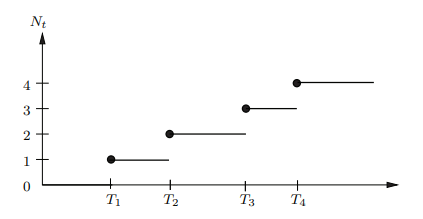
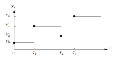
The sum of the rates out of state $i$ is denoted by $q_{i}$. A typical sample path of $X$ is shown in Figure 1.6. The process jumps at times $T_{1}, T_{2}, \ldots$ to states $Y_{1}, Y_{2}, \ldots$, staying some length of time in each state.

More precisely, a Markov jump process $X$ behaves (under suitable regularity conditions; see [3]) as follows:

  1. Given its past, the probability that $X$ jumps from its current state $i$ to state $j$ is $K_{i j}=q_{i j} / q_{i}$.
  2. The amount of time that $X$ spends in state $j$ has an exponential distribution with mean $1 / q_{j}$, independent of its past history.

The first statement implies that the process $\left{Y_{n}\right}$ is in fact a Markov chain, with transition matrix $K=\left(K_{i j}\right)$.

A convenient way to describe a Markov jump process is through its transition rate graph. This is similar to a transition graph for Markov chains. The states are represented by the nodes of the graph, and a transition rate from state $i$ to $j$ is indicated by an arrow from $i$ to $j$ with weight $q_{i j}$.

统计代写|蒙特卡洛方法代写monte carlo method代考|Birth-and-Death Process

A birth-and-death process is a Markov jump process with a transition rate graph of the form given in Figure 1.7. Imagine that $X_{t}$ represents the total number of individuals in a population at time $t$. Jumps to the right correspond to births, and jumps to the left to deaths. The birth rates $\left{b_{i}\right}$ and the death rates $\left{d_{i}\right}$ may differ from state to state. Many applications of Markov chains involve processes of this kind. Note that the process jumps from one state to

the next according to a Markov chain with transition probabilities $K_{0,1}=1$, $K_{i, i+1}=b_{i} /\left(b_{i}+d_{i}\right)$, and $K_{i, i-1}=d_{i} /\left(b_{i}+d_{i}\right), i=1,2, \ldots$. Moreover, it spends an $\operatorname{Exp}\left(b_{0}\right)$ amount of time in state 0 and $\operatorname{Exp}\left(b_{i}+d_{i}\right)$ in the other states.
Limiting Behavior We now formulate the continuous-time analogues of (1.34) and Theorem 1.13.2. Irreducibility and recurrence for Markov jump processes are defined in the same way as for Markov chains. For simplicity, we assume that $\mathscr{E}={1,2, \ldots}$. If $X$ is a recurrent and irreducible Markov jump process, then regardless of $i$,
$$
\lim {t \rightarrow \infty} \mathbb{P}\left(X{t}=j \mid X_{0}=i\right)=\pi_{j}
$$
for some number $\pi_{j} \geqslant 0$. Moreover, $\pi=\left(\pi_{1}, \pi_{2}, \ldots\right)$ is the solution to
$$
\sum_{j \neq i} \pi_{i} q_{i j}=\sum_{j \neq i} \pi_{j} q_{j i}, \quad \text { for all } i=1, \ldots, m
$$
with $\sum_{j} \pi_{j}=1$, if such a solution exists, in which case all states are positive recurrent. If such a solution does not exist, all $\pi_{j}$ are 0 .

As in the Markov chain case, $\left{\pi_{j}\right}$ is called the limiting distribution of $X$ and is usually identified with the row vector $\pi$. Any solution $\pi$ of (1.42) with $\sum_{j} \pi_{j}=1$ is called a stationary distribution, since taking it as the initial distribution of the Markov jump process renders the process stationary.

统计代写|蒙特卡洛方法代写monte carlo method代考|GAUSSIAN PROCESSES

The normal distribution is also called the Gaussian distribution. Gaussian processes are generalizations of multivariate normal random vectors (discussed in Section 1.10). Specifically, a stochastic process $\left{X_{t}, t \in \mathscr{T}\right}$ is said to be Gaussian if all its finite-dimensional distributions are Gaussian. That is, if for any choice of $n$ and $t_{1}, \ldots, t_{n} \in \mathscr{T}$, it holds that
$$
\left(X_{t_{1}}, \ldots, X_{t_{n}}\right)^{\top} \sim \mathrm{N}(\boldsymbol{\mu}, \Sigma)
$$
for some expectation vector $\boldsymbol{\mu}$ and covariance matrix $\Sigma$ (both of which depend on the choice of $\left.t_{1}, \ldots, t_{n}\right)$. Equivalently, $\left{X_{t}, t \in \mathscr{T}\right}$ is Gaussian if any linear combination $\sum_{i=1}^{n} b_{i} X_{t_{i}}$ has a normal distribution. Note that a Gaussian process is determined completely by its expectation function $\mu_{t}=\mathbb{E}\left[X_{t}\right], t \in \mathscr{T}$, and covariance function $\Sigma_{s, t}=\operatorname{Cov}\left(X_{s}, X_{t}\right), s, t \in \mathscr{T}$.

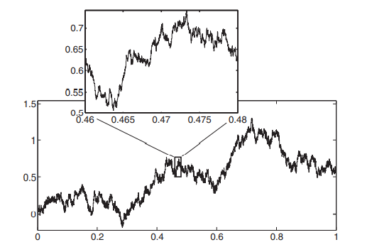
The Wiener process can be defined as a Gaussian process $\left{X_{t}, t \geqslant 0\right}$ with expectation function $\mu_{t}=0$ for all $t$ and covariance function $\Sigma_{s, t}=s$ for $0 \leqslant s \leqslant t$. The Wiener process has many fascinating properties (e.g., [11]). For example, it is a Markov process (i.e., it satisfies the Markov property $(1.30)$ ) with continuous sample paths that are nowhere differentiable. Moreover, the increments $X_{t}-X_{s}$ over intervals $[s, t]$ are independent and normally distributed. Specifically, for any $t_{1}<t_{2} \leqslant t_{3}<t_{4}$,
$$
X_{t_{4}}-X_{t_{3}} \quad \text { and } \quad X_{t_{2}}-X_{t_{1}}
$$
are independent random variables, and for all $t \geqslant s \geqslant 0$,
$$
X_{t}-X_{s} \sim \mathrm{N}(0, t-s) .
$$
This leads to a simple simulation procedure for Wiener processes, which is discussed in Section 2.8.

统计代写|蒙特卡洛方法代写monte carlo method代考| Markov Jump Processes

monte carlo method代写

统计代写|蒙特卡洛方法代写monte carlo method代考|Markov Jump Processes

马尔可夫跳跃过程X=\left{X_{t}, t \geqslant 0\right}X=\left{X_{t}, t \geqslant 0\right}可以看作是马尔可夫链和泊松过程的连续时间推广。马尔科夫性质(1.30)现在读
磷(X吨+s=X吨+s∣X在=X在,在⩽吨)=磷(X吨+s=X吨+s∣X吨=X吨).
与马尔可夫链的情况一样,通常假设过程是时间齐次的,即磷(X吨+s=j∣X吨=一世)不依赖于吨. 将此概率表示为磷s(一世,j). 一个重要的量是转换率q一世j从状态一世到j, 定义为一世≠j作为
q一世j=林吨↓0磷吨(一世,j)吨.
州外费率总和一世表示为q一世. 一个典型的样本路径X如图 1.6 所示。过程有时会跳跃吨1,吨2,…给各州是1,是2,…,在每个状态停留一段时间。

更准确地说,马尔可夫跳跃过程X行为(在合适的规律性条件下;参见 [3])如下:

  1. 鉴于它的过去,概率X从当前状态跳转一世陈述j是ķ一世j=q一世j/q一世.
  2. 的时间量X在州花费j具有均值的指数分布1/qj,独立于其过去的历史。

第一条语句意味着该过程\left{Y_{n}\right}\left{Y_{n}\right}实际上是一个马尔可夫链,带有转移矩阵ķ=(ķ一世j).

描述马尔可夫跳跃过程的一种方便方法是通过其转换率图。这类似于马尔可夫链的转移图。状态由图的节点表示,以及状态的转换率一世到j用箭头表示一世到j有重量q一世j.

统计代写|蒙特卡洛方法代写monte carlo method代考|Birth-and-Death Process

生死过程是一个马尔可夫跳跃过程,其转换率图的形式如图 1.7 所示。想象一下X吨表示在某个时间人口中的个体总数吨. 向右跳对应出生,向左跳对应死亡。出生率\left{b_{i}\right}\left{b_{i}\right}和死亡率\left{d_{i}\right}\left{d_{i}\right}可能因州而异。马尔可夫链的许多应用都涉及这种过程。请注意,该过程从一种状态跳转到

下一个根据具有转移概率的马尔可夫链ķ0,1=1, ķ一世,一世+1=b一世/(b一世+d一世), 和ķ一世,一世−1=d一世/(b一世+d一世),一世=1,2,…. 此外,它花费了一个经验⁡(b0)处于状态 0 的时间量和经验⁡(b一世+d一世)在其他州。
限制行为 我们现在制定 (1.34) 和定理 1.13.2 的连续时间类似物。马尔可夫跳跃过程的不可约性和重复性的定义与马尔可夫链的定义方式相同。为简单起见,我们假设和=1,2,…. 如果X是一个循环且不可约的马尔可夫跳跃过程,则不管一世,
林吨→∞磷(X吨=j∣X0=一世)=圆周率j
对于一些数字圆周率j⩾0. 而且,圆周率=(圆周率1,圆周率2,…)是解决方案
∑j≠一世圆周率一世q一世j=∑j≠一世圆周率jqj一世, 对全部 一世=1,…,米
和∑j圆周率j=1,如果存在这样的解决方案,在这种情况下,所有状态都是正循环的。如果没有这样的解决方案,所有圆周率j是 0 。

就像马尔可夫链的情况一样,\左{\pi_{j}\右}\左{\pi_{j}\右}称为极限分布X并且通常用行向量标识圆周率. 任何解决方案圆周率(1.42) 的∑j圆周率j=1称为平稳分布,因为将其作为马尔可夫跳跃过程的初始分布会使过程平稳。

统计代写|蒙特卡洛方法代写monte carlo method代考|GAUSSIAN PROCESSES

正态分布也称为高斯分布。高斯过程是多元正态随机向量的推广(在 1.10 节中讨论)。具体来说,一个随机过程\left{X_{t}, t \in \mathscr{T}\right}\left{X_{t}, t \in \mathscr{T}\right}如果其所有有限维分布都是高斯分布,则称其为高斯分布。也就是说,如果对于任何选择n和吨1,…,吨n∈吨, 它认为
(X吨1,…,X吨n)⊤∼ñ(μ,Σ)
对于一些期望向量μ和协方差矩阵Σ(两者都取决于选择吨1,…,吨n). 等效地,\left{X_{t}, t \in \mathscr{T}\right}\left{X_{t}, t \in \mathscr{T}\right}如果有任何线性组合,则为高斯∑一世=1nb一世X吨一世具有正态分布。请注意,高斯过程完全由其期望函数决定μ吨=和[X吨],吨∈吨, 和协方差函数Σs,吨=这⁡(Xs,X吨),s,吨∈吨.

维纳过程可以定义为高斯过程\left{X_{t}, t \geqslant 0\right}\left{X_{t}, t \geqslant 0\right}有期望函数μ吨=0对全部吨和协方差函数Σs,吨=s为了0⩽s⩽吨. 维纳过程有许多令人着迷的特性(例如,[11])。例如,它是一个马尔科夫过程(即满足马尔科夫性质(1.30)) 具有无处可微的连续样本路径。此外,增量X吨−Xs间隔时间[s,吨]是独立且正态分布的。具体来说,对于任何吨1<吨2⩽吨3<吨4,
X吨4−X吨3 和 X吨2−X吨1
是独立的随机变量,并且对于所有吨⩾s⩾0,
X吨−Xs∼ñ(0,吨−s).
这导致了一个简单的维纳过程模拟过程,这将在第 2.8 节中讨论。

统计代写|蒙特卡洛方法代写monte carlo method代考 请认准statistics-lab™

统计代写请认准statistics-lab™. statistics-lab™为您的留学生涯保驾护航。

金融工程代写

金融工程是使用数学技术来解决金融问题。金融工程使用计算机科学、统计学、经济学和应用数学领域的工具和知识来解决当前的金融问题,以及设计新的和创新的金融产品。

非参数统计代写

非参数统计指的是一种统计方法,其中不假设数据来自于由少数参数决定的规定模型;这种模型的例子包括正态分布模型和线性回归模型。

广义线性模型代考

广义线性模型(GLM)归属统计学领域,是一种应用灵活的线性回归模型。该模型允许因变量的偏差分布有除了正态分布之外的其它分布。

术语 广义线性模型(GLM)通常是指给定连续和/或分类预测因素的连续响应变量的常规线性回归模型。它包括多元线性回归,以及方差分析和方差分析(仅含固定效应)。

有限元方法代写

有限元方法(FEM)是一种流行的方法,用于数值解决工程和数学建模中出现的微分方程。典型的问题领域包括结构分析、传热、流体流动、质量运输和电磁势等传统领域。

有限元是一种通用的数值方法,用于解决两个或三个空间变量的偏微分方程(即一些边界值问题)。为了解决一个问题,有限元将一个大系统细分为更小、更简单的部分,称为有限元。这是通过在空间维度上的特定空间离散化来实现的,它是通过构建对象的网格来实现的:用于求解的数值域,它有有限数量的点。边界值问题的有限元方法表述最终导致一个代数方程组。该方法在域上对未知函数进行逼近。[1] 然后将模拟这些有限元的简单方程组合成一个更大的方程系统,以模拟整个问题。然后,有限元通过变化微积分使相关的误差函数最小化来逼近一个解决方案。

tatistics-lab作为专业的留学生服务机构,多年来已为美国、英国、加拿大、澳洲等留学热门地的学生提供专业的学术服务,包括但不限于Essay代写,Assignment代写,Dissertation代写,Report代写,小组作业代写,Proposal代写,Paper代写,Presentation代写,计算机作业代写,论文修改和润色,网课代做,exam代考等等。写作范围涵盖高中,本科,研究生等海外留学全阶段,辐射金融,经济学,会计学,审计学,管理学等全球99%专业科目。写作团队既有专业英语母语作者,也有海外名校硕博留学生,每位写作老师都拥有过硬的语言能力,专业的学科背景和学术写作经验。我们承诺100%原创,100%专业,100%准时,100%满意。

随机分析代写


随机微积分是数学的一个分支,对随机过程进行操作。它允许为随机过程的积分定义一个关于随机过程的一致的积分理论。这个领域是由日本数学家伊藤清在第二次世界大战期间创建并开始的。

时间序列分析代写

随机过程,是依赖于参数的一组随机变量的全体,参数通常是时间。 随机变量是随机现象的数量表现,其时间序列是一组按照时间发生先后顺序进行排列的数据点序列。通常一组时间序列的时间间隔为一恒定值(如1秒,5分钟,12小时,7天,1年),因此时间序列可以作为离散时间数据进行分析处理。研究时间序列数据的意义在于现实中,往往需要研究某个事物其随时间发展变化的规律。这就需要通过研究该事物过去发展的历史记录,以得到其自身发展的规律。

回归分析代写

多元回归分析渐进(Multiple Regression Analysis Asymptotics)属于计量经济学领域,主要是一种数学上的统计分析方法,可以分析复杂情况下各影响因素的数学关系,在自然科学、社会和经济学等多个领域内应用广泛。

MATLAB代写

MATLAB 是一种用于技术计算的高性能语言。它将计算、可视化和编程集成在一个易于使用的环境中,其中问题和解决方案以熟悉的数学符号表示。典型用途包括:数学和计算算法开发建模、仿真和原型制作数据分析、探索和可视化科学和工程图形应用程序开发,包括图形用户界面构建MATLAB 是一个交互式系统,其基本数据元素是一个不需要维度的数组。这使您可以解决许多技术计算问题,尤其是那些具有矩阵和向量公式的问题,而只需用 C 或 Fortran 等标量非交互式语言编写程序所需的时间的一小部分。MATLAB 名称代表矩阵实验室。MATLAB 最初的编写目的是提供对由 LINPACK 和 EISPACK 项目开发的矩阵软件的轻松访问,这两个项目共同代表了矩阵计算软件的最新技术。MATLAB 经过多年的发展,得到了许多用户的投入。在大学环境中,它是数学、工程和科学入门和高级课程的标准教学工具。在工业领域,MATLAB 是高效研究、开发和分析的首选工具。MATLAB 具有一系列称为工具箱的特定于应用程序的解决方案。对于大多数 MATLAB 用户来说非常重要,工具箱允许您学习应用专业技术。工具箱是 MATLAB 函数(M 文件)的综合集合,可扩展 MATLAB 环境以解决特定类别的问题。可用工具箱的领域包括信号处理、控制系统、神经网络、模糊逻辑、小波、仿真等。

R语言代写问卷设计与分析代写
PYTHON代写回归分析与线性模型代写
MATLAB代写方差分析与试验设计代写
STATA代写机器学习/统计学习代写
SPSS代写计量经济学代写
EVIEWS代写时间序列分析代写
EXCEL代写深度学习代写
SQL代写各种数据建模与可视化代写

统计代写|蒙特卡洛方法代写monte carlo method代考| Classification of States

如果你也在 怎样代写蒙特卡洛方法学monte carlo method这个学科遇到相关的难题,请随时右上角联系我们的24/7代写客服。

蒙特卡洛方法,或称蒙特卡洛实验,是一类广泛的计算算法,依靠重复随机抽样来获得数值结果。其基本概念是利用随机性来解决原则上可能是确定性的问题。

statistics-lab™ 为您的留学生涯保驾护航 在代写蒙特卡洛方法学monte carlo method方面已经树立了自己的口碑, 保证靠谱, 高质且原创的统计Statistics代写服务。我们的专家在代写蒙特卡洛方法学monte carlo method代写方面经验极为丰富,各种代写蒙特卡洛方法学monte carlo method相关的作业也就用不着说。

我们提供的蒙特卡洛方法学monte carlo method及其相关学科的代写,服务范围广, 其中包括但不限于:

  • Statistical Inference 统计推断
  • Statistical Computing 统计计算
  • Advanced Probability Theory 高等概率论
  • Advanced Mathematical Statistics 高等数理统计学
  • (Generalized) Linear Models 广义线性模型
  • Statistical Machine Learning 统计机器学习
  • Longitudinal Data Analysis 纵向数据分析
  • Foundations of Data Science 数据科学基础
统计代写|蒙特卡洛方法代写monte carlo method代考| Classification of States

统计代写|蒙特卡洛方法代写monte carlo method代考|Classification of States

Let $X$ be a Markov chain with discrete state space $E$ and transition matrix $P$. We can characterize the relations between states in the following way: If states $i$ and $j$ are such that $P^{t}(i, j)>0$ for some $t \geqslant 0$, we say that $i$ leads to $j$ and write $i \rightarrow j$. We say that $i$ and $j$ communicate if $i \rightarrow j$ and $j \rightarrow i$, and write $i \leftrightarrow j$. Using the relation ” $\leftrightarrow “$ “, we can divide $\mathscr{E}$ into equivalence classes such that all the states in an equivalence class communicate with each other but not with any state outside that class. If there is only one equivalent class $(=\mathscr{E})$, the Markov chain is said to be irreducible. If a set of states $\mathscr{A}$ is such that $\sum_{j \in \mathscr{A}} P(i, j)=1$ for all $i \in \mathscr{A}$, then $\mathscr{A}$ is called a closed set. A state $i$ is called an absorbing state if ${i}$ is closed. For example, in the transition graph depicted in Figure 1.5, the equivalence classes are ${1,2},{3}$, and ${4,5}$. Class ${1,2}$ is the only closed set: the Markov chain cannot escape from it. If state 1 were missing, state 2 would be absorbing. In Example $1.10$ the Markov chain is irreducible since all states communicate.

Another classification of states is obtained by observing the system from a local point of view. In particular, let $T$ denote the time the chain first visits state $j$, or first returns to $j$ if it started there, and let $N_{j}$ denote the total number of visits to $j$ from time 0 on. We write $\mathbb{P}{j}(A)$ for $\mathbb{P}\left(A \mid X{0}=j\right)$ for any event $A$. We denote the corresponding expectation operator by $\mathbb{E}{j}$. State $j$ is called a recurrent state if $\mathbb{P}{j}(T<\infty)=1$; otherwise, $j$ is called transient. A recurrent state is called positive recurrent if $\mathbb{E}{j}[T]<\infty$; otherwise, it is called null recurrent. Finally, a state is said to be periodic, with period $\delta$, if $\delta \geqslant 2$ is the largest integer for which $\mathbb{P}{j}(T=n \delta$ for some $n \geqslant 1)=1$; otherwise, it is called aperiodic. For example, in Figure $1.5$ states 1 and 2 are recurrent, and the other states are transient. All these states are aperiodic. The states of the random walk of Example $1.10$ are periodic with period 2 .

It can be shown that recurrence and transience are class properties. In particular, if $i \leftrightarrow j$, then $i$ recurrent (transient) $\Leftrightarrow j$ recurrent (transient). Thus, in an irreducible Markov chain, one state being recurrent implies that all other states are also recurrent. And if one state is transient, then so are all the others.

统计代写|蒙特卡洛方法代写monte carlo method代考|Limiting Behavior

The limiting or “steady-state” behavior of Markov chains as $t \rightarrow \infty$ is of considerable interest and importance, and this type of behavior is often simpler to describe and analyze than the “transient” behavior of the chain for fixed $t$. It can be shown (see, for example, [3]) that in an irreducible, aperiodic Markov chain with transition matrix $P$ the $t$-step probabilities converge to a constant that does not depend on the initial state. More specifically,
$$
\lim {t \rightarrow \infty} P^{t}(i, j)=\pi{j}
$$
for some number $0 \leqslant \pi_{j} \leqslant 1$. Moreover, $\pi_{j}>0$ if $j$ is positive recurrent and $\pi_{j}=0$ otherwise. The intuitive reason behind this result is that the process “forgets” where it was initially if it goes on long enough. This is true for both finite and countably infinite Markov chains. The numbers $\left{\pi_{j}, j \in \mathscr{E}\right}$ form the limiting distribution of the Markov chain, provided that $\pi_{j} \geqslant 0$ and $\sum_{j} \pi_{j}=1$. Note that these conditions are not always satisfied: they are clearly not satisfied if the Markov chain is transient, and they may not be satisfied if the Markov chain is recurrent (i.e., when the states are null-recurrent). The following theorem gives a method for obtaining limiting distributions. Here we assume for simplicity that $\mathscr{E}={0,1,2, \ldots}$. The limiting distribution is identified with the row vector $\pi=$ $\left(\pi_{0}, \pi_{1}, \ldots\right)$

Theorem 1.13.2 For an irreducible, aperiodic Markov chain with transition matrix $P$, if the limiting distribution $\pi$ exists, then it is uniquely determined by the solution of
$$
\pi=\pi P
$$
with $\pi_{j} \geqslant 0$ and $\sum_{j} \pi_{j}=1$. Conversely, if there exists a positive row vector $\pi$ satisfying (1.35) and summing up to 1 , then $\pi$ is the limiting distribution of the Markov chain. Moreover, in that case, $\pi_{j}>0$ for all $j$ and all states are positive recurrent.

Proof: (Sketch) For the case where $\mathscr{E}$ is finite, the result is simply a consequence of (1.33). Namely, with $\pi^{(0)}$ being the $i$-th unit vector, we have
$$
P^{t+1}(i, j)=\left(\pi^{(0)} P^{t} P\right)(j)=\sum_{k \in \mathcal{E}} P^{t}(i, k) P(k, j)
$$
Letting $t \rightarrow \infty$, we obtain (1.35) from (1.34), provided that we can change the order of the limit and the summation. To show uniqueness, suppose that another vector $\mathbf{y}$, with $y_{j} \geqslant 0$ and $\sum_{j} y_{j}=1$, satisfies $\mathbf{y}=\mathbf{y} P$. Then it is easy to show by induction that $\mathbf{y}=\mathbf{y} P^{t}$, for every $t$. Hence, letting $t \rightarrow \infty$, we obtain for every $j$
$$
y_{j}=\sum_{i} y_{i} \pi_{j}=\pi_{j},
$$
since the $\left{y_{j}\right}$ sum up to unity. We omit the proof of the converse statement.

统计代写|蒙特卡洛方法代写monte carlo method代考|Random Walk on the Positive Integers

This is a slightly different random walk than the one in Example 1.10. Let $X$ be a random walk on $\mathscr{E}={0,1,2, \ldots}$ with transition matrix
$$
P=\left(\begin{array}{cccccc}
q & p & 0 & \ldots & & \
q & 0 & p & 0 & \ldots & \
0 & q & 0 & p & 0 & \cdots \
\vdots & \ddots & \ddots & \ddots & \ddots & \ddots
\end{array}\right)
$$
where $0<p<1$ and $q=1-p . X_{l}$ could represent, for example, the number of customers who are waiting in a queue at time $t$.

All states can be reached from each other, so the chain is irreducible and every state is either recurrent or transient. The equation $\pi=\pi P$ becomes
$$
\begin{aligned}
&\pi_{0}=q \pi_{0}+q \pi_{1} \
&\pi_{1}=p \pi_{0}+q \pi_{2} \
&\pi_{2}=p \pi_{1}+q \pi_{3} \
&\pi_{3}=p \pi_{2}+q \pi_{4}
\end{aligned}
$$
and so on. We can solve this set of equation sequentially. If we let $r=p / q$, then we can express the $\pi_{1}, \pi_{2}, \ldots$ in terms of $\pi_{0}$ and $r$ as
$$
\pi_{j}=r^{j} \pi_{0}, j=0,1,2, \ldots
$$

统计代写|蒙特卡洛方法代写monte carlo method代考| Classification of States

monte carlo method代写

统计代写|蒙特卡洛方法代写monte carlo method代考|Classification of States

让X是具有离散状态空间的马尔可夫链和和转移矩阵磷. 我们可以用以下方式描述状态之间的关系:如果状态一世和j是这样的磷吨(一世,j)>0对于一些吨⩾0, 我们说一世导致j和写一世→j. 我们说一世和j沟通如果一世→j和j→一世, 和写一世↔j. 使用关系”↔““,我们可以分和等价类,使得等价类中的所有状态都相互通信,但不与该类之外的任何状态通信。如果只有一个等效类(=和),马尔可夫链是不可约的。如果一组状态一种是这样的∑j∈一种磷(一世,j)=1对全部一世∈一种, 然后一种称为闭集。一个状态一世被称为吸收状态,如果一世已经关闭。例如,在图 1.5 中描述的转移图中,等价类是1,2,3, 和4,5. 班级1,2是唯一的闭集:马尔可夫链无法从中逃脱。如果状态 1 缺失,则状态 2 将被吸收。在示例中1.10马尔可夫链是不可约的,因为所有状态都可以通信。

另一种状态分类是通过从局部角度观察系统获得的。特别是,让吨表示链首次访问状态的时间j, 或首先返回j如果它从那里开始,让ñj表示访问的总次数j从时间 0 开始。我们写磷j(一种)为了磷(一种∣X0=j)对于任何事件一种. 我们将相应的期望算子表示为和j. 状态j称为循环状态,如果磷j(吨<∞)=1; 除此以外,j称为瞬态。一个循环状态称为正循环,如果和j[吨]<∞; 否则,称为空循环。最后,一个状态被称为是周期性的,其中周期d, 如果d⩾2是最大的整数磷j(吨=nd对于一些n⩾1)=1; 否则,它被称为非周期性的。例如,在图1.5状态 1 和 2 是循环的,其他状态是瞬态的。所有这些状态都是非周期性的。Example 的随机游走的状态1.10周期为 2 。

可以证明,递归和瞬态是类属性。特别是,如果一世↔j, 然后一世经常性(瞬态)⇔j经常性(瞬态)。因此,在不可约马尔可夫链中,一个状态是循环的意味着所有其他状态也是循环的。如果一种状态是短暂的,那么其他所有状态也是如此。

统计代写|蒙特卡洛方法代写monte carlo method代考|Limiting Behavior

马尔可夫链的限制或“稳态”行为吨→∞具有相当大的兴趣和重要性,并且这种类型的行为通常比固定链的“瞬态”行为更易于描述和分析吨. 可以证明(例如,参见 [3])在具有转移矩阵的不可约非周期马尔可夫链中磷这吨步概率收敛到一个不依赖于初始状态的常数。进一步来说,
林吨→∞磷吨(一世,j)=圆周率j
对于一些数字0⩽圆周率j⩽1. 而且,圆周率j>0如果j是阳性复发和圆周率j=0除此以外。这个结果背后的直观原因是,如果持续足够长的时间,该过程会“忘记”最初的位置。这对于有限和可数无限的马尔可夫链都是正确的。号码\left{\pi_{j}, j \in \mathscr{E}\right}\left{\pi_{j}, j \in \mathscr{E}\right}形成马尔可夫链的极限分布,前提是圆周率j⩾0和∑j圆周率j=1. 请注意,这些条件并不总是满足:如果马尔可夫链是瞬态的,它们显然不满足,如果马尔可夫链是循环的(即,当状态为空循环时),它们可能不满足。下面的定理给出了一种获得极限分布的方法。在这里,为了简单起见,我们假设和=0,1,2,…. 极限分布用行向量标识圆周率= (圆周率0,圆周率1,…)

定理 1.13.2 对于具有转移矩阵的不可约非周期马尔可夫链磷, 如果极限分布圆周率存在,那么它是由解唯一确定的
圆周率=圆周率磷
和圆周率j⩾0和∑j圆周率j=1. 反之,如果存在正的行向量圆周率满足 (1.35) 并求和为 1 ,则圆周率是马尔可夫链的极限分布。此外,在那种情况下,圆周率j>0对全部j并且所有状态都是正循环的。

证明:(草图)和是有限的,结果只是(1.33)的结果。即,与圆周率(0)作为一世-th 单位向量,我们有
磷吨+1(一世,j)=(圆周率(0)磷吨磷)(j)=∑ķ∈和磷吨(一世,ķ)磷(ķ,j)
让吨→∞,我们从 (1.34) 得到 (1.35),前提是我们可以改变极限和求和的顺序。为了显示唯一性,假设另一个向量是, 和是j⩾0和∑j是j=1, 满足是=是磷. 那么很容易通过归纳证明是=是磷吨, 对于每个吨. 因此,让吨→∞, 我们得到每个j
是j=∑一世是一世圆周率j=圆周率j,
自从\left{y_{j}\right}\left{y_{j}\right}总结为统一。我们省略了相反陈述的证明。

统计代写|蒙特卡洛方法代写monte carlo method代考|Random Walk on the Positive Integers

这与示例 1.10 中的随机游走略有不同。让X随意走和=0,1,2,…有转移矩阵
磷=(qp0… q0p0… 0q0p0⋯ ⋮⋱⋱⋱⋱⋱)
在哪里0<p<1和q=1−p.Xl例如,可以表示在某个时间排队等候的客户数量吨.

所有状态都可以相互到达,因此链是不可约的,每个状态要么是循环的,要么是短暂的。方程圆周率=圆周率磷变成
圆周率0=q圆周率0+q圆周率1 圆周率1=p圆周率0+q圆周率2 圆周率2=p圆周率1+q圆周率3 圆周率3=p圆周率2+q圆周率4
等等。我们可以依次求解这组方程。如果我们让r=p/q,那么我们可以表达圆周率1,圆周率2,…按照圆周率0和r作为
圆周率j=rj圆周率0,j=0,1,2,…

统计代写|蒙特卡洛方法代写monte carlo method代考 请认准statistics-lab™

统计代写请认准statistics-lab™. statistics-lab™为您的留学生涯保驾护航。

金融工程代写

金融工程是使用数学技术来解决金融问题。金融工程使用计算机科学、统计学、经济学和应用数学领域的工具和知识来解决当前的金融问题,以及设计新的和创新的金融产品。

非参数统计代写

非参数统计指的是一种统计方法,其中不假设数据来自于由少数参数决定的规定模型;这种模型的例子包括正态分布模型和线性回归模型。

广义线性模型代考

广义线性模型(GLM)归属统计学领域,是一种应用灵活的线性回归模型。该模型允许因变量的偏差分布有除了正态分布之外的其它分布。

术语 广义线性模型(GLM)通常是指给定连续和/或分类预测因素的连续响应变量的常规线性回归模型。它包括多元线性回归,以及方差分析和方差分析(仅含固定效应)。

有限元方法代写

有限元方法(FEM)是一种流行的方法,用于数值解决工程和数学建模中出现的微分方程。典型的问题领域包括结构分析、传热、流体流动、质量运输和电磁势等传统领域。

有限元是一种通用的数值方法,用于解决两个或三个空间变量的偏微分方程(即一些边界值问题)。为了解决一个问题,有限元将一个大系统细分为更小、更简单的部分,称为有限元。这是通过在空间维度上的特定空间离散化来实现的,它是通过构建对象的网格来实现的:用于求解的数值域,它有有限数量的点。边界值问题的有限元方法表述最终导致一个代数方程组。该方法在域上对未知函数进行逼近。[1] 然后将模拟这些有限元的简单方程组合成一个更大的方程系统,以模拟整个问题。然后,有限元通过变化微积分使相关的误差函数最小化来逼近一个解决方案。

tatistics-lab作为专业的留学生服务机构,多年来已为美国、英国、加拿大、澳洲等留学热门地的学生提供专业的学术服务,包括但不限于Essay代写,Assignment代写,Dissertation代写,Report代写,小组作业代写,Proposal代写,Paper代写,Presentation代写,计算机作业代写,论文修改和润色,网课代做,exam代考等等。写作范围涵盖高中,本科,研究生等海外留学全阶段,辐射金融,经济学,会计学,审计学,管理学等全球99%专业科目。写作团队既有专业英语母语作者,也有海外名校硕博留学生,每位写作老师都拥有过硬的语言能力,专业的学科背景和学术写作经验。我们承诺100%原创,100%专业,100%准时,100%满意。

随机分析代写


随机微积分是数学的一个分支,对随机过程进行操作。它允许为随机过程的积分定义一个关于随机过程的一致的积分理论。这个领域是由日本数学家伊藤清在第二次世界大战期间创建并开始的。

时间序列分析代写

随机过程,是依赖于参数的一组随机变量的全体,参数通常是时间。 随机变量是随机现象的数量表现,其时间序列是一组按照时间发生先后顺序进行排列的数据点序列。通常一组时间序列的时间间隔为一恒定值(如1秒,5分钟,12小时,7天,1年),因此时间序列可以作为离散时间数据进行分析处理。研究时间序列数据的意义在于现实中,往往需要研究某个事物其随时间发展变化的规律。这就需要通过研究该事物过去发展的历史记录,以得到其自身发展的规律。

回归分析代写

多元回归分析渐进(Multiple Regression Analysis Asymptotics)属于计量经济学领域,主要是一种数学上的统计分析方法,可以分析复杂情况下各影响因素的数学关系,在自然科学、社会和经济学等多个领域内应用广泛。

MATLAB代写

MATLAB 是一种用于技术计算的高性能语言。它将计算、可视化和编程集成在一个易于使用的环境中,其中问题和解决方案以熟悉的数学符号表示。典型用途包括:数学和计算算法开发建模、仿真和原型制作数据分析、探索和可视化科学和工程图形应用程序开发,包括图形用户界面构建MATLAB 是一个交互式系统,其基本数据元素是一个不需要维度的数组。这使您可以解决许多技术计算问题,尤其是那些具有矩阵和向量公式的问题,而只需用 C 或 Fortran 等标量非交互式语言编写程序所需的时间的一小部分。MATLAB 名称代表矩阵实验室。MATLAB 最初的编写目的是提供对由 LINPACK 和 EISPACK 项目开发的矩阵软件的轻松访问,这两个项目共同代表了矩阵计算软件的最新技术。MATLAB 经过多年的发展,得到了许多用户的投入。在大学环境中,它是数学、工程和科学入门和高级课程的标准教学工具。在工业领域,MATLAB 是高效研究、开发和分析的首选工具。MATLAB 具有一系列称为工具箱的特定于应用程序的解决方案。对于大多数 MATLAB 用户来说非常重要,工具箱允许您学习应用专业技术。工具箱是 MATLAB 函数(M 文件)的综合集合,可扩展 MATLAB 环境以解决特定类别的问题。可用工具箱的领域包括信号处理、控制系统、神经网络、模糊逻辑、小波、仿真等。

R语言代写问卷设计与分析代写
PYTHON代写回归分析与线性模型代写
MATLAB代写方差分析与试验设计代写
STATA代写机器学习/统计学习代写
SPSS代写计量经济学代写
EVIEWS代写时间序列分析代写
EXCEL代写深度学习代写
SQL代写各种数据建模与可视化代写

统计代写|蒙特卡洛方法代写monte carlo method代考| MARKOV PROCESSES

如果你也在 怎样代写蒙特卡洛方法学monte carlo method这个学科遇到相关的难题,请随时右上角联系我们的24/7代写客服。

蒙特卡洛方法,或称蒙特卡洛实验,是一类广泛的计算算法,依靠重复随机抽样来获得数值结果。其基本概念是利用随机性来解决原则上可能是确定性的问题。

statistics-lab™ 为您的留学生涯保驾护航 在代写蒙特卡洛方法学monte carlo method方面已经树立了自己的口碑, 保证靠谱, 高质且原创的统计Statistics代写服务。我们的专家在代写蒙特卡洛方法学monte carlo method代写方面经验极为丰富,各种代写蒙特卡洛方法学monte carlo method相关的作业也就用不着说。

我们提供的蒙特卡洛方法学monte carlo method及其相关学科的代写,服务范围广, 其中包括但不限于:

  • Statistical Inference 统计推断
  • Statistical Computing 统计计算
  • Advanced Probability Theory 高等概率论
  • Advanced Mathematical Statistics 高等数理统计学
  • (Generalized) Linear Models 广义线性模型
  • Statistical Machine Learning 统计机器学习
  • Longitudinal Data Analysis 纵向数据分析
  • Foundations of Data Science 数据科学基础
统计代写|蒙特卡洛方法代写monte carlo method代考| MARKOV PROCESSES

统计代写|蒙特卡洛方法代写monte carlo method代考|MARKOV PROCESSES

Markov processes are stochastic processes whose futures are conditionally independent of their pasts given their present values. More formally, a stochastic process $\left{X_{t}, t \in \mathscr{T}\right}$, with $\mathscr{T} \subseteq \mathbb{R}$, is called a Markov process if, for every $s>0$ and $t$,
$$
\left(X_{t+s} \mid X_{u}, u \leqslant t\right) \sim\left(X_{t+s} \mid X_{t}\right)
$$
In other words, the conditional distribution of the future variable $X_{t+s}$, given the entire past of the process $\left{X_{u}, u \leqslant t\right}$, is the same as the conditional distribution of $X_{t+s}$ given only the present $X_{t}$. That is, in order to predict future states, we only need to know the present one. Property (1.30) is called the Markov property.
Depending on the index set $\mathscr{T}$ and state space $\mathscr{E}$ (the set of all values the $\left{X_{t}\right}$ can take), Markov processes come in many different forms. A Markov process with a discrete index set is called a Markov chain. A Markov process with a discrete state space and a continuous index set (such as $\mathbb{R}$ or $\mathbb{R}_{+}$) is called a Markov jump process.

统计代写|蒙特卡洛方法代写monte carlo method代考|Markov Chains

Consider a Markov chain $X=\left{X_{t}, t \in \mathbb{N}\right}$ with a discrete (i.e., countable) state space $\mathscr{E}$. In this case the Markov property (1.30) is
$$
\mathbb{P}\left(X_{t+1}=x_{t+1} \mid X_{0}=x_{0}, \ldots, X_{t}=x_{t}\right)=\mathbb{P}\left(X_{t+1}=x_{t+1} \mid X_{t}=x_{t}\right)
$$
for all $x_{0}, \ldots, x_{t+1}, \in \mathscr{E}$ and $t \in \mathbb{N}$. We restrict ourselves to Markov chains for which the conditional probabilities
$$
\mathbb{P}\left(X_{t+1}=j \mid X_{t}=i\right), i, j \in \mathscr{E}
$$
are independent of the time $t$. Such chains are called time-homogeneous. The probabilities in (1.32) are called the (one-step) transition probabilities of $X$. The distribution of $X_{0}$ is called the initial distribution of the Markov chain. The one-step transition probabilities and the initial distribution completely specify the distribution of $X$. Namely, we have by the product rule (1.4) and the Markov property (1.30),
$$
\begin{aligned}
&\mathbb{P}\left(X_{U}=x_{U}, \ldots, X_{t}=x_{t}\right) \
&\quad=\mathbb{P}\left(X_{0}=x_{0}\right) \mathbb{P}\left(X_{1}=x_{1} \mid X_{0}=x_{0}\right) \cdots \mathbb{P}\left(X_{t}=x_{t} \mid X_{0}=x_{0}, \ldots X_{t-1}=x_{t-1}\right) \
&\quad=\mathbb{P}\left(X_{0}=x_{0}\right) \mathbb{P}\left(X_{1}=x_{1} \mid X_{0}=x_{0}\right) \cdots \mathbb{P}\left(X_{t}=x_{t} \mid X_{t-1}=x_{t-1}\right) .
\end{aligned}
$$
Since $\mathscr{E}$ is countable, we can arrange the one-step transition probabilities in an array. This array is called the (one-step) transition matrix of $X$. We usually denote it by $P$. For example, when $\mathscr{E}={0,1,2, \ldots}$, the transition matrix $P$ has the form
$$
P=\left(\begin{array}{cccc}
p_{00} & p_{01} & p_{02} & \cdots \
p_{10} & p_{11} & p_{12} & \cdots \
p_{20} & p_{21} & p_{22} & \cdots \
\vdots & \vdots & \vdots & \ddots
\end{array}\right) \text {. }
$$
Note that the elements in every row are positive and sum up to unity.
Another convenient way to describe a Markov chain $X$ is through its transition graph. States are indicated by the nodes of the graph, and a strictly positive $(>0)$ transition probability $p_{i j}$ from state $i$ to $j$ is indicated by an arrow from $i$ to $j$ with weight $p_{i j}$.

统计代写|蒙特卡洛方法代写monte carlo method代考|Random Walk on the Integers

Let $p$ be a number between 0 and 1 . The Markov chain $X$ with state space $\mathbb{Z}$ and transition matrix $P$ defined by
$$
P(i, i+1)=p, \quad P(i, i-1)=\bar{q}=1-\bar{p}, \quad \text { for all } i \in \mathbb{Z}
$$
is called a random walk on the integers. Let $X$ start at $0 ;$ thus, $\mathbb{P}\left(X_{0}=0\right)=1$. The corresponding transition graph is given in Figure 1.4. Starting at 0 , the chain takes subsequent steps to the right with probability $p$ and to the left with probability $q$.

We show next how to calculate the probability that, starting from state $i$ at some (discrete) time $t$, we are in $j$ at (discrete) time $t+s$, that is, the probability $\mathbb{P}\left(X_{t+s}=j \mid X_{t}=i\right)$. For clarity, let us assume that $\mathscr{E}={1,2, \ldots, m}$ for some fixed $m$, so that $P$ is an $m \times m$ matrix. For $t=0,1,2, \ldots$, define the row vector
$$
\boldsymbol{\pi}^{(t)}=\left(\mathbb{P}\left(X_{t}=1\right), \ldots, \mathbb{P}\left(X_{t}=m\right)\right)
$$
We call $\pi^{(t)}$ the distribution vector, or simply the distribution, of $X$ at time $t$ and $\pi^{(0)}$ the initial distribution of $X$. The following result shows that the $t$-step probabilities can be found simply by matrix multiplication.
Theorem 1.13.1 The distribution of $X$ at time $t$ is given by
$$
\pi^{(t)}=\pi^{(0)} P^{t}
$$
for all $t=0,1, \ldots .$ (Here $P^{0}$ denotes the identity matrix.)
Proof: The proof is by induction. Equality (1.33) holds for $t=0$ by definition. Suppose that this equality is true for some $t=0,1, \ldots$. We have
$$
\mathbb{P}\left(X_{t+1}=k\right)=\sum_{i=1}^{m} \mathbb{P}\left(X_{t+1}=k \mid X_{t}=i\right) \mathbb{P}\left(X_{t}=i\right)
$$
But (1.33) is assumed to be true for $t$, so $\mathbb{P}\left(X_{t}=i\right)$ is the $i$-th element of $\pi^{(0)} P^{t}$. Moreover, $\mathbb{P}\left(X_{t+1}=k \mid X_{t}=i\right)$ is the $(i, k)$-th element of $P$. Therefore, for every $k$,
$$
\sum_{i=1}^{m} \mathbb{P}\left(X_{t+1}=k \mid X_{t}=i\right) \mathbb{P}\left(X_{t}=i\right)=\sum_{i=1}^{m} P(i, k)\left(\boldsymbol{\pi}^{(0)} P^{t}\right)(i)
$$
which is just the $k$-th element of $\pi^{(0)} P^{t+1}$. This completes the induction step, and thus the theorem is proved.

By taking $\pi^{(0)}$ as the $i$-th unit vector, $\mathbf{e}{i}$, the $t$-step transition probabilities can be found as $\mathbb{P}\left(X{t}=j \mid X_{0}=i\right)=\left(\mathbf{e}_{i} P^{t}\right)(j)=P^{t}(i, j)$, which is the $(i, j)$-th element of matrix $P^{t}$. Ihus, to find the $t$-step transition probabilities, we just have to compute the $t$-th power of $P$.

统计代写|蒙特卡洛方法代写monte carlo method代考| MARKOV PROCESSES

monte carlo method代写

统计代写|蒙特卡洛方法代写monte carlo method代考|MARKOV PROCESSES

马尔可夫过程是随机过程,在给定当前值的情况下,其未来有条件地独立于其过去。更正式地说,一个随机过程\left{X_{t}, t \in \mathscr{T}\right}\left{X_{t}, t \in \mathscr{T}\right}, 和吨⊆R,称为马尔可夫过程,如果,对于每个s>0和吨,
(X吨+s∣X在,在⩽吨)∼(X吨+s∣X吨)
换句话说,未来变量的条件分布X吨+s,给定整个过程的过去\left{X_{u}, u \leqslant t\right}\left{X_{u}, u \leqslant t\right}, 与条件分布相同X吨+s只给现在X吨. 也就是说,为了预测未来的状态,我们只需要知道现在的状态。属性(1.30)称为马尔可夫属性。
取决于索引集吨和状态空间和(所有值的集合\left{X_{t}\right}\left{X_{t}\right}可以采取),马尔可夫过程有许多不同的形式。具有离散索引集的马尔可夫过程称为马尔可夫链。具有离散状态空间和连续索引集的马尔可夫过程(例如R或者R+) 称为马尔科夫跳跃过程。

统计代写|蒙特卡洛方法代写monte carlo method代考|Markov Chains

考虑马尔可夫链X=\left{X_{t}, t \in \mathbb{N}\right}X=\left{X_{t}, t \in \mathbb{N}\right}具有离散(即可数)状态空间和. 在这种情况下,马尔可夫属性 (1.30) 是
磷(X吨+1=X吨+1∣X0=X0,…,X吨=X吨)=磷(X吨+1=X吨+1∣X吨=X吨)
对全部X0,…,X吨+1,∈和和吨∈ñ. 我们将自己限制在条件概率的马尔可夫链上
磷(X吨+1=j∣X吨=一世),一世,j∈和
与时间无关吨. 这样的链被称为时间均匀的。(1.32)中的概率称为(一步)转移概率X. 的分布X0称为马尔可夫链的初始分布。一步转移概率和初始分布完全指定了X. 即,我们有乘积规则(1.4)和马尔可夫性质(1.30),
磷(X在=X在,…,X吨=X吨) =磷(X0=X0)磷(X1=X1∣X0=X0)⋯磷(X吨=X吨∣X0=X0,…X吨−1=X吨−1) =磷(X0=X0)磷(X1=X1∣X0=X0)⋯磷(X吨=X吨∣X吨−1=X吨−1).
自从和是可数的,我们可以将单步转移概率排列在一个数组中。这个数组被称为(一步)转移矩阵X. 我们通常用磷. 例如,当和=0,1,2,…, 转移矩阵磷有形式
磷=(p00p01p02⋯ p10p11p12⋯ p20p21p22⋯ ⋮⋮⋮⋱). 
请注意,每一行中的元素都是正数并且总和为一。
另一种描述马尔可夫链的便捷方式X是通过它的转移图。状态由图中的节点表示,严格的正(>0)转移概率p一世j从状态一世到j用箭头表示一世到j有重量p一世j.

统计代写|蒙特卡洛方法代写monte carlo method代考|Random Walk on the Integers

让p是介于 0 和 1 之间的数字。马尔可夫链X有状态空间从和转移矩阵磷被定义为
磷(一世,一世+1)=p,磷(一世,一世−1)=q¯=1−p¯, 对全部 一世∈从
被称为整数上的随机游走。让X开始于0;因此,磷(X0=0)=1. 相应的转换图如图​​ 1.4 所示。从 0 开始,链以概率向右执行后续步骤p并以概率向左q.

我们接下来展示如何计算从状态开始的概率一世在某个(离散的)时间吨, 我们在j在(离散)时间吨+s,也就是概率磷(X吨+s=j∣X吨=一世). 为了清楚起见,让我们假设和=1,2,…,米对于一些固定的米, 以便磷是一个米×米矩阵。为了吨=0,1,2,…, 定义行向量
圆周率(吨)=(磷(X吨=1),…,磷(X吨=米))
我们称之为圆周率(吨)的分布向量,或简称分布,X有时吨和圆周率(0)的初始分布X. 下面的结果表明,吨-step 概率可以通过矩阵乘法简单地找到。
定理 1.13.1 的分布X有时吨是(谁)给的
圆周率(吨)=圆周率(0)磷吨
对全部吨=0,1,….(这里磷0表示单位矩阵。)
证明:证明是通过归纳。等式 (1.33) 成立吨=0根据定义。假设这个等式对某些人是正确的吨=0,1,…. 我们有
磷(X吨+1=ķ)=∑一世=1米磷(X吨+1=ķ∣X吨=一世)磷(X吨=一世)
但是(1.33)被假定为对吨, 所以磷(X吨=一世)是个一世-第一个元素圆周率(0)磷吨. 而且,磷(X吨+1=ķ∣X吨=一世)是个(一世,ķ)-第一个元素磷. 因此,对于每个ķ,
∑一世=1米磷(X吨+1=ķ∣X吨=一世)磷(X吨=一世)=∑一世=1米磷(一世,ķ)(圆周率(0)磷吨)(一世)
这只是ķ-第一个元素圆周率(0)磷吨+1. 这样就完成了归纳步骤,从而证明了定理。

通过采取圆周率(0)作为一世-th 单位向量,和一世, 这吨-step转移概率可以找到磷(X吨=j∣X0=一世)=(和一世磷吨)(j)=磷吨(一世,j), 哪一个是(一世,j)- 矩阵的第一个元素磷吨. 伊胡斯,找到吨-step 转移概率,我们只需要计算吨- 次方磷.

统计代写|蒙特卡洛方法代写monte carlo method代考 请认准statistics-lab™

统计代写请认准statistics-lab™. statistics-lab™为您的留学生涯保驾护航。

金融工程代写

金融工程是使用数学技术来解决金融问题。金融工程使用计算机科学、统计学、经济学和应用数学领域的工具和知识来解决当前的金融问题,以及设计新的和创新的金融产品。

非参数统计代写

非参数统计指的是一种统计方法,其中不假设数据来自于由少数参数决定的规定模型;这种模型的例子包括正态分布模型和线性回归模型。

广义线性模型代考

广义线性模型(GLM)归属统计学领域,是一种应用灵活的线性回归模型。该模型允许因变量的偏差分布有除了正态分布之外的其它分布。

术语 广义线性模型(GLM)通常是指给定连续和/或分类预测因素的连续响应变量的常规线性回归模型。它包括多元线性回归,以及方差分析和方差分析(仅含固定效应)。

有限元方法代写

有限元方法(FEM)是一种流行的方法,用于数值解决工程和数学建模中出现的微分方程。典型的问题领域包括结构分析、传热、流体流动、质量运输和电磁势等传统领域。

有限元是一种通用的数值方法,用于解决两个或三个空间变量的偏微分方程(即一些边界值问题)。为了解决一个问题,有限元将一个大系统细分为更小、更简单的部分,称为有限元。这是通过在空间维度上的特定空间离散化来实现的,它是通过构建对象的网格来实现的:用于求解的数值域,它有有限数量的点。边界值问题的有限元方法表述最终导致一个代数方程组。该方法在域上对未知函数进行逼近。[1] 然后将模拟这些有限元的简单方程组合成一个更大的方程系统,以模拟整个问题。然后,有限元通过变化微积分使相关的误差函数最小化来逼近一个解决方案。

tatistics-lab作为专业的留学生服务机构,多年来已为美国、英国、加拿大、澳洲等留学热门地的学生提供专业的学术服务,包括但不限于Essay代写,Assignment代写,Dissertation代写,Report代写,小组作业代写,Proposal代写,Paper代写,Presentation代写,计算机作业代写,论文修改和润色,网课代做,exam代考等等。写作范围涵盖高中,本科,研究生等海外留学全阶段,辐射金融,经济学,会计学,审计学,管理学等全球99%专业科目。写作团队既有专业英语母语作者,也有海外名校硕博留学生,每位写作老师都拥有过硬的语言能力,专业的学科背景和学术写作经验。我们承诺100%原创,100%专业,100%准时,100%满意。

随机分析代写


随机微积分是数学的一个分支,对随机过程进行操作。它允许为随机过程的积分定义一个关于随机过程的一致的积分理论。这个领域是由日本数学家伊藤清在第二次世界大战期间创建并开始的。

时间序列分析代写

随机过程,是依赖于参数的一组随机变量的全体,参数通常是时间。 随机变量是随机现象的数量表现,其时间序列是一组按照时间发生先后顺序进行排列的数据点序列。通常一组时间序列的时间间隔为一恒定值(如1秒,5分钟,12小时,7天,1年),因此时间序列可以作为离散时间数据进行分析处理。研究时间序列数据的意义在于现实中,往往需要研究某个事物其随时间发展变化的规律。这就需要通过研究该事物过去发展的历史记录,以得到其自身发展的规律。

回归分析代写

多元回归分析渐进(Multiple Regression Analysis Asymptotics)属于计量经济学领域,主要是一种数学上的统计分析方法,可以分析复杂情况下各影响因素的数学关系,在自然科学、社会和经济学等多个领域内应用广泛。

MATLAB代写

MATLAB 是一种用于技术计算的高性能语言。它将计算、可视化和编程集成在一个易于使用的环境中,其中问题和解决方案以熟悉的数学符号表示。典型用途包括:数学和计算算法开发建模、仿真和原型制作数据分析、探索和可视化科学和工程图形应用程序开发,包括图形用户界面构建MATLAB 是一个交互式系统,其基本数据元素是一个不需要维度的数组。这使您可以解决许多技术计算问题,尤其是那些具有矩阵和向量公式的问题,而只需用 C 或 Fortran 等标量非交互式语言编写程序所需的时间的一小部分。MATLAB 名称代表矩阵实验室。MATLAB 最初的编写目的是提供对由 LINPACK 和 EISPACK 项目开发的矩阵软件的轻松访问,这两个项目共同代表了矩阵计算软件的最新技术。MATLAB 经过多年的发展,得到了许多用户的投入。在大学环境中,它是数学、工程和科学入门和高级课程的标准教学工具。在工业领域,MATLAB 是高效研究、开发和分析的首选工具。MATLAB 具有一系列称为工具箱的特定于应用程序的解决方案。对于大多数 MATLAB 用户来说非常重要,工具箱允许您学习应用专业技术。工具箱是 MATLAB 函数(M 文件)的综合集合,可扩展 MATLAB 环境以解决特定类别的问题。可用工具箱的领域包括信号处理、控制系统、神经网络、模糊逻辑、小波、仿真等。

R语言代写问卷设计与分析代写
PYTHON代写回归分析与线性模型代写
MATLAB代写方差分析与试验设计代写
STATA代写机器学习/统计学习代写
SPSS代写计量经济学代写
EVIEWS代写时间序列分析代写
EXCEL代写深度学习代写
SQL代写各种数据建模与可视化代写

统计代写|蒙特卡洛方法代写monte carlo method代考| JOINTLY NORMAL RANDOM VARIABLES

如果你也在 怎样代写蒙特卡洛方法学monte carlo method这个学科遇到相关的难题,请随时右上角联系我们的24/7代写客服。

蒙特卡洛方法,或称蒙特卡洛实验,是一类广泛的计算算法,依靠重复随机抽样来获得数值结果。其基本概念是利用随机性来解决原则上可能是确定性的问题。

statistics-lab™ 为您的留学生涯保驾护航 在代写蒙特卡洛方法学monte carlo method方面已经树立了自己的口碑, 保证靠谱, 高质且原创的统计Statistics代写服务。我们的专家在代写蒙特卡洛方法学monte carlo method代写方面经验极为丰富,各种代写蒙特卡洛方法学monte carlo method相关的作业也就用不着说。

我们提供的蒙特卡洛方法学monte carlo method及其相关学科的代写,服务范围广, 其中包括但不限于:

  • Statistical Inference 统计推断
  • Statistical Computing 统计计算
  • Advanced Probability Theory 高等概率论
  • Advanced Mathematical Statistics 高等数理统计学
  • (Generalized) Linear Models 广义线性模型
  • Statistical Machine Learning 统计机器学习
  • Longitudinal Data Analysis 纵向数据分析
  • Foundations of Data Science 数据科学基础
统计代写|蒙特卡洛方法代写monte carlo method代考| JOINTLY NORMAL RANDOM VARIABLES

统计代写|蒙特卡洛方法代写monte carlo method代考|JOINTLY NORMAL RANDOM VARIABLES

It is helpful to view normally distributed random variables as simple transformations of standard normal – that is, $\mathrm{N}(0,1)$-distributed – random variables. In particular, let $X \sim \mathrm{N}(0,1)$. Then $X$ has density $f_{X}$ given by
$$
f_{X}(x)=\frac{1}{\sqrt{2 \pi}} \mathrm{e}^{-\frac{x^{2}}{2}} .
$$
Now consider the transformation $Z=\mu+\sigma X$. Then, by (1.15), $Z$ has density
$$
f_{Z}(z)=\frac{1}{\sqrt{2 \pi \sigma^{2}}} \mathrm{e}^{-\frac{(z-\mu)^{2}}{2 \sigma^{2}}} .
$$
In other words, $Z \sim \mathrm{N}\left(\mu, \sigma^{2}\right)$. We can also state this as follows: if $Z \sim \mathrm{N}\left(\mu, \sigma^{2}\right)$, then $(Z-\mu) / \sigma \sim \mathrm{N}(0,1)$. This procedure is called standardization.

We now generalize this to $n$ dimensions. Let $X_{1}, \ldots, X_{n}$ be independent and standard normal random variables. The joint pdf of $\mathbf{X}=\left(X_{1}, \ldots, X_{n}\right)^{\top}$ is given by
$$
f_{\mathbf{X}}(\mathbf{x})=(2 \pi)^{-n / 2} \mathrm{e}^{-\frac{1}{2} \mathbf{x}^{\top} \mathbf{x}}, \quad \mathbf{x} \in \mathbb{R}^{n} .
$$
Consider the affine transformation (i.e., a linear transformation plus a constant vector)
$$
\mathbf{Z}=\boldsymbol{\mu}+B \mathbf{X}
$$
for some $m \times n$ matrix $B$. Note that, by Theorem 1.8.1, Z has expectation vector $\boldsymbol{\mu}$ and covariance matrix $\Sigma=B B^{\top}$. Any random vector of the form (1.23) is said to have a jointly normal or multivariate normal distribution. We write $\mathbf{Z} \sim N(\boldsymbol{\mu}, \Sigma)$. Suppose that $B$ is an invertible $n \times n$ matrix. Then, by (1.19), the density of $\mathbf{Y}=\mathbf{Z}-\boldsymbol{\mu}$ is given by
$$
f_{\mathbf{Y}}(\mathbf{y})=\frac{1}{|B| \sqrt{(2 \pi)^{n}}} \mathrm{e}^{-\frac{1}{2}\left(B^{-1} \mathbf{y}\right)^{\top} B^{-1} \mathbf{y}}=\frac{1}{|B| \sqrt{(2 \pi)^{n}}} \mathrm{e}^{-\frac{1}{2} \mathbf{y}^{\top}\left(B^{-1}\right)^{\top} B^{-1} \mathbf{y}} .
$$
We have $|B|=\sqrt{|\Sigma|}$ and $\left(B^{-1}\right)^{\top} B^{-1}=\left(B^{\top}\right)^{-1} B^{-1}=\left(B B^{\top}\right)^{-1}=\Sigma^{-1}$, so that
$$
f_{\mathbf{Y}}(\mathbf{y})=\frac{1}{\sqrt{(2 \pi)^{n}|\Sigma|}} \mathrm{e}^{-\frac{1}{2} \mathbf{y}^{\top} \Sigma^{-1} \mathbf{y}} .
$$
Because $\mathbf{Z}$ is obtained from $\mathbf{Y}$ by simply adding a constant vector $\boldsymbol{\mu}$, we have $f_{\mathbf{Z}}(\mathbf{z})=f_{\mathbf{Y}}(\mathbf{z}-\boldsymbol{\mu})$, and therefore
$$
f_{\mathbf{Z}}(\mathbf{z})=\frac{1}{\sqrt{(2 \pi)^{n}|\Sigma|}} \mathrm{e}^{-\frac{1}{2}(\mathbf{z}-\boldsymbol{\mu})^{\top} \Sigma^{-1}(\mathbf{z}-\mu)}, \quad \mathbf{z} \in \mathbb{R}^{n} .
$$
Note that this formula is very similar to that of the one-dimensional case.
Conversely, given a covariance matrix $\Sigma=\left(\sigma_{i j}\right)$, there exists a unique lower triangular matrix
$$
B=\left(\begin{array}{cccc}
b_{11} & 0 & \cdots & 0 \
b_{21} & b_{22} & \cdots & 0 \
\vdots & \vdots & & \vdots \
b_{n 1} & b_{n 2} & \cdots & b_{n n}
\end{array}\right)
$$
such that $\Sigma=B B^{\top}$. This matrix can be obtained efficiently via the Cholesky square root method; see Section A.1 of the Appendix.

统计代写|蒙特卡洛方法代写monte carlo method代考|LIMIT THEOREMS

We briefly discuss two of the main results in probability: the law of large numbers and the central limit theorem. Both are associated with sums of independent random variables.

Let $X_{1}, X_{2}, \ldots$ be iid random variables with expectation $\mu$ and variance $\sigma^{2}$. For each $n$, let $S_{n}=X_{1}+\cdots+X_{n}$. Since $X_{1}, X_{2}, \ldots$ are iid, we have $\mathbb{E}\left[S_{n}\right]=n \mathbb{E}\left[X_{1}\right]=$ $n \mu$ and $\operatorname{Var}\left(S_{n}\right)=n \operatorname{Var}\left(X_{1}\right)=n \sigma^{2}$.

The law of large numbers states that $S_{n} / n$ is close to $\mu$ for large $n$. Here is the more precise statement.

Theorem 1.11.1 (Strong Law of Large Numbers) If $X_{1}, \ldots, X_{n}$ are iid with expectation $\mu$, then
$$
\mathbb{P}\left(\lim {n \rightarrow \infty} \frac{S{n}}{n}=\mu\right)=1
$$
The central limit theorem describes the limiting distribution of $S_{n}$ (or $S_{n} / n$ ), and it applies to both continuous and discrete random variables. Loosely, it states that the random sum $S_{n}$ has a distribution that is approximately normal, when $n$ is large. The more precise statement is given next.

Theorem 1.11.2 (Central Limit Theorem) If $X_{1}, \ldots, X_{n}$ are iid with expectation $\mu$ and variance $\sigma^{2}<\infty$, then for all $x \in \mathbb{R}$,
$$
\lim {n \rightarrow \infty} \mathbb{P}\left(\frac{S{n}-n \mu}{\sigma \sqrt{n}} \leqslant x\right)=\Phi(x),
$$
where $\Phi$ is the cdf of the standard normal distribution.
In other words, $S_{n}$ has a distribution that is approximately normal, with expectation $n \mu$ and variance $n \sigma^{2}$. To see the central limit theorem in action, consider Figure 1.2. The left part shows the pdfs of $S_{1}, \ldots, S_{4}$ for the case where the $\left{X_{i}\right}$ have a $U[0,1]$ distribution. The right part shows the same for the $\operatorname{Exp}(1)$ distribution. We clearly see convergence to a bell-shaped curve, characteristic of the normal distribution.

统计代写|蒙特卡洛方法代写monte carlo method代考|POISSON PROCESSES

The Poisson process is used to model certain kinds of arrivals or patterns. Imagine, for example, a telescope that can detect individual photons from a faraway galaxy. The photons arrive at random times $T_{1}, T_{2}, \ldots .$ Let $N_{t}$ denote the number of arrivals in the time interval $[0, t]$, that is, $N_{t}=\sup \left{k: T_{k} \leqslant t\right}$. Note that the number of arrivals in an interval $I=(a, b]$ is given by $N_{b}-N_{a}$. We will also denote it by $N(a, b]$. A sample path of the arrival counting process $\left{N_{t}, t \geqslant 0\right}$ is given in Figure 1.3.

For this particular arrival process, one would assume that the number of arrivals in an interval $(a, b)$ is independent of the number of arrivals in interval $(c, d)$ when the two intervals do not intersect. Such considerations lead to the following definition:

Definition 1.12.1 (Poisson Process) An arrival counting process $N=\left{N_{t}\right}$ is called a Poisson process with rate $\lambda>0$ if
(a) The numbers of points in nonoverlapping intervals are independent.
(b) The number of points in interval $I$ has a Poisson distribution with mean $\lambda \times \operatorname{length}(I)$.

统计代写|蒙特卡洛方法代写monte carlo method代考| JOINTLY NORMAL RANDOM VARIABLES

monte carlo method代写

统计代写|蒙特卡洛方法代写monte carlo method代考|JOINTLY NORMAL RANDOM VARIABLES

将正态分布的随机变量视为标准正态的简单变换是有帮助的——也就是说,ñ(0,1)-分布式——随机变量。特别是,让X∼ñ(0,1). 然后X有密度FX由
FX(X)=12圆周率和−X22.
现在考虑转换从=μ+σX. 然后,由 (1.15),从有密度
F从(和)=12圆周率σ2和−(和−μ)22σ2.
换句话说,从∼ñ(μ,σ2). 我们也可以这样表述:如果从∼ñ(μ,σ2), 然后(从−μ)/σ∼ñ(0,1). 这个过程称为标准化。

我们现在将其推广到n方面。让X1,…,Xn是独立的标准正态随机变量。联合pdfX=(X1,…,Xn)⊤是(谁)给的
FX(X)=(2圆周率)−n/2和−12X⊤X,X∈Rn.
考虑仿射变换(即线性变换加常数向量)
从=μ+乙X
对于一些米×n矩阵乙. 请注意,根据定理 1.8.1,Z 具有期望向量μ和协方差矩阵Σ=乙乙⊤. 任何形式为 (1.23) 的随机向量都被称为具有联合正态分布或多元正态分布。我们写从∼ñ(μ,Σ). 假设乙是可逆的n×n矩阵。然后,由(1.19),密度是=从−μ是(谁)给的
F是(是)=1|乙|(2圆周率)n和−12(乙−1是)⊤乙−1是=1|乙|(2圆周率)n和−12是⊤(乙−1)⊤乙−1是.
我们有|乙|=|Σ|和(乙−1)⊤乙−1=(乙⊤)−1乙−1=(乙乙⊤)−1=Σ−1, 以便
F是(是)=1(2圆周率)n|Σ|和−12是⊤Σ−1是.
因为从是从是通过简单地添加一个常数向量μ, 我们有F从(和)=F是(和−μ),因此
F从(和)=1(2圆周率)n|Σ|和−12(和−μ)⊤Σ−1(和−μ),和∈Rn.
请注意,此公式与一维情况的公式非常相似。
相反,给定一个协方差矩阵Σ=(σ一世j), 存在唯一的下三角矩阵
乙=(b110⋯0 b21b22⋯0 ⋮⋮⋮ bn1bn2⋯bnn)
这样Σ=乙乙⊤. 该矩阵可以通过 Cholesky 平方根方法有效地获得;见附录 A.1 节。

统计代写|蒙特卡洛方法代写monte carlo method代考|LIMIT THEOREMS

我们简要讨论概率的两个主要结果:大数定律和中心极限定理。两者都与独立随机变量的总和有关。

让X1,X2,…是具有期望的独立同分布随机变量μ和方差σ2. 对于每个n, 让小号n=X1+⋯+Xn. 自从X1,X2,…是 iid,我们有和[小号n]=n和[X1]= nμ和曾是⁡(小号n)=n曾是⁡(X1)=nσ2.

大数定律指出小号n/n接近μ对于大n. 这是更准确的说法。

定理 1.11.1(大数强定律)如果X1,…,Xn充满期待μ, 然后
磷(林n→∞小号nn=μ)=1
中心极限定理描述了小号n(或者小号n/n),它适用于连续和离散的随机变量。松散地,它指出随机和小号n具有近似正态分布,当n很大。接下来给出更准确的陈述。

定理 1.11.2(中心极限定理)如果X1,…,Xn充满期待μ和方差σ2<∞, 那么对于所有X∈R,
林n→∞磷(小号n−nμσn⩽X)=披(X),
在哪里披是标准正态分布的 cdf。
换句话说,小号n具有近似正态分布,具有期望nμ和方差nσ2. 要查看实际的中心极限定理,请考虑图 1.2。左边部分显示了pdf小号1,…,小号4对于这种情况\left{X_{i}\right}\left{X_{i}\right}有一个在[0,1]分配。右侧部分显示相同的经验⁡(1)分配。我们清楚地看到收敛到钟形曲线,这是正态分布的特征。

统计代写|蒙特卡洛方法代写monte carlo method代考|POISSON PROCESSES

泊松过程用于对某些类型的到达或模式进行建模。例如,想象一个可以探测到来自遥远星系的单个光子的望远镜。光子随机到达吨1,吨2,….让ñ吨表示时间间隔内的到达次数[0,吨], 那是,N_{t}=\sup \left{k: T_{k} \leqslant t\right}N_{t}=\sup \left{k: T_{k} \leqslant t\right}. 注意一个区间内的到达次数一世=(一种,b]是(谁)给的ñb−ñ一种. 我们也将其表示为ñ(一种,b]. 到达计数过程的示例路径\left{N_{t}, t \geqslant 0\right}\left{N_{t}, t \geqslant 0\right}如图 1.3 所示。

对于这个特定的到达过程,可以假设一个区间内的到达次数(一种,b)与区间内的到达次数无关(C,d)当两个区间不相交时。这些考虑导致了以下定义:

定义 1.12.1(泊松过程)到达计数过程N=\left{N_{t}\right}N=\left{N_{t}\right}称为具有速率的泊松过程λ>0如果
(a) 非重叠区间中的点数是独立的。
(b) 区间点数一世具有均值的泊松分布λ×长度⁡(一世).

统计代写|蒙特卡洛方法代写monte carlo method代考 请认准statistics-lab™

统计代写请认准statistics-lab™. statistics-lab™为您的留学生涯保驾护航。

金融工程代写

金融工程是使用数学技术来解决金融问题。金融工程使用计算机科学、统计学、经济学和应用数学领域的工具和知识来解决当前的金融问题,以及设计新的和创新的金融产品。

非参数统计代写

非参数统计指的是一种统计方法,其中不假设数据来自于由少数参数决定的规定模型;这种模型的例子包括正态分布模型和线性回归模型。

广义线性模型代考

广义线性模型(GLM)归属统计学领域,是一种应用灵活的线性回归模型。该模型允许因变量的偏差分布有除了正态分布之外的其它分布。

术语 广义线性模型(GLM)通常是指给定连续和/或分类预测因素的连续响应变量的常规线性回归模型。它包括多元线性回归,以及方差分析和方差分析(仅含固定效应)。

有限元方法代写

有限元方法(FEM)是一种流行的方法,用于数值解决工程和数学建模中出现的微分方程。典型的问题领域包括结构分析、传热、流体流动、质量运输和电磁势等传统领域。

有限元是一种通用的数值方法,用于解决两个或三个空间变量的偏微分方程(即一些边界值问题)。为了解决一个问题,有限元将一个大系统细分为更小、更简单的部分,称为有限元。这是通过在空间维度上的特定空间离散化来实现的,它是通过构建对象的网格来实现的:用于求解的数值域,它有有限数量的点。边界值问题的有限元方法表述最终导致一个代数方程组。该方法在域上对未知函数进行逼近。[1] 然后将模拟这些有限元的简单方程组合成一个更大的方程系统,以模拟整个问题。然后,有限元通过变化微积分使相关的误差函数最小化来逼近一个解决方案。

tatistics-lab作为专业的留学生服务机构,多年来已为美国、英国、加拿大、澳洲等留学热门地的学生提供专业的学术服务,包括但不限于Essay代写,Assignment代写,Dissertation代写,Report代写,小组作业代写,Proposal代写,Paper代写,Presentation代写,计算机作业代写,论文修改和润色,网课代做,exam代考等等。写作范围涵盖高中,本科,研究生等海外留学全阶段,辐射金融,经济学,会计学,审计学,管理学等全球99%专业科目。写作团队既有专业英语母语作者,也有海外名校硕博留学生,每位写作老师都拥有过硬的语言能力,专业的学科背景和学术写作经验。我们承诺100%原创,100%专业,100%准时,100%满意。

随机分析代写


随机微积分是数学的一个分支,对随机过程进行操作。它允许为随机过程的积分定义一个关于随机过程的一致的积分理论。这个领域是由日本数学家伊藤清在第二次世界大战期间创建并开始的。

时间序列分析代写

随机过程,是依赖于参数的一组随机变量的全体,参数通常是时间。 随机变量是随机现象的数量表现,其时间序列是一组按照时间发生先后顺序进行排列的数据点序列。通常一组时间序列的时间间隔为一恒定值(如1秒,5分钟,12小时,7天,1年),因此时间序列可以作为离散时间数据进行分析处理。研究时间序列数据的意义在于现实中,往往需要研究某个事物其随时间发展变化的规律。这就需要通过研究该事物过去发展的历史记录,以得到其自身发展的规律。

回归分析代写

多元回归分析渐进(Multiple Regression Analysis Asymptotics)属于计量经济学领域,主要是一种数学上的统计分析方法,可以分析复杂情况下各影响因素的数学关系,在自然科学、社会和经济学等多个领域内应用广泛。

MATLAB代写

MATLAB 是一种用于技术计算的高性能语言。它将计算、可视化和编程集成在一个易于使用的环境中,其中问题和解决方案以熟悉的数学符号表示。典型用途包括:数学和计算算法开发建模、仿真和原型制作数据分析、探索和可视化科学和工程图形应用程序开发,包括图形用户界面构建MATLAB 是一个交互式系统,其基本数据元素是一个不需要维度的数组。这使您可以解决许多技术计算问题,尤其是那些具有矩阵和向量公式的问题,而只需用 C 或 Fortran 等标量非交互式语言编写程序所需的时间的一小部分。MATLAB 名称代表矩阵实验室。MATLAB 最初的编写目的是提供对由 LINPACK 和 EISPACK 项目开发的矩阵软件的轻松访问,这两个项目共同代表了矩阵计算软件的最新技术。MATLAB 经过多年的发展,得到了许多用户的投入。在大学环境中,它是数学、工程和科学入门和高级课程的标准教学工具。在工业领域,MATLAB 是高效研究、开发和分析的首选工具。MATLAB 具有一系列称为工具箱的特定于应用程序的解决方案。对于大多数 MATLAB 用户来说非常重要,工具箱允许您学习应用专业技术。工具箱是 MATLAB 函数(M 文件)的综合集合,可扩展 MATLAB 环境以解决特定类别的问题。可用工具箱的领域包括信号处理、控制系统、神经网络、模糊逻辑、小波、仿真等。

R语言代写问卷设计与分析代写
PYTHON代写回归分析与线性模型代写
MATLAB代写方差分析与试验设计代写
STATA代写机器学习/统计学习代写
SPSS代写计量经济学代写
EVIEWS代写时间序列分析代写
EXCEL代写深度学习代写
SQL代写各种数据建模与可视化代写

统计代写|蒙特卡洛方法代写monte carlo method代考|FUNCTIONS OF RANDOM VARIABLES

如果你也在 怎样代写蒙特卡洛方法学monte carlo method这个学科遇到相关的难题,请随时右上角联系我们的24/7代写客服。

蒙特卡洛方法,或称蒙特卡洛实验,是一类广泛的计算算法,依靠重复随机抽样来获得数值结果。其基本概念是利用随机性来解决原则上可能是确定性的问题。

statistics-lab™ 为您的留学生涯保驾护航 在代写蒙特卡洛方法学monte carlo method方面已经树立了自己的口碑, 保证靠谱, 高质且原创的统计Statistics代写服务。我们的专家在代写蒙特卡洛方法学monte carlo method代写方面经验极为丰富,各种代写蒙特卡洛方法学monte carlo method相关的作业也就用不着说。

我们提供的蒙特卡洛方法学monte carlo method及其相关学科的代写,服务范围广, 其中包括但不限于:

  • Statistical Inference 统计推断
  • Statistical Computing 统计计算
  • Advanced Probability Theory 高等概率论
  • Advanced Mathematical Statistics 高等数理统计学
  • (Generalized) Linear Models 广义线性模型
  • Statistical Machine Learning 统计机器学习
  • Longitudinal Data Analysis 纵向数据分析
  • Foundations of Data Science 数据科学基础
Probability Distribution for a Discrete Random Variable | CK-12 Foundation
统计代写|蒙特卡洛方法代写monte carlo method代考|FUNCTIONS OF RANDOM VARIABLES

统计代写|蒙特卡洛方法代写monte carlo method代考|FUNCTIONS OF RANDOM VARIABLES

Suppose that $X_{1}, \ldots, X_{n}$ are measurements of a random experiment. Often we are only interested in certain functions of the measurements rather than the individual measurements. Here are some examples.
EXAMPLE $1.5$
Let $X$ be a continuous random variable with pdf $f_{X}$ and let $Z=a X+b$, where $a \neq 0$. We wish to determine the pdf $f_{Z}$ of $Z$. Suppose that $a>0$. We have for any $z$
$$
F_{Z}(z)=\mathbb{P}(Z \leqslant z)=\mathbb{P}(X \leqslant(z-b) / a)=F_{X}((z-b) / a) .
$$
Differentiating this with respect to $z$ gives $f_{Z}(z)=f_{X}((z-b) / a) / a$. For $a<0$ we similarly obtain $f_{Z}(z)=f_{X}((z-b) / a) /(-a)$. Thus, in general,
$$
f_{Z}(z)=\frac{1}{|a|} f_{X}\left(\frac{z-b}{a}\right) .
$$
EXAMPLE $1.6$
Generalizing the previous example, suppose that $Z=g(X)$ for some monotonically increasing function $g$. To find the pdf of $Z$ from that of $X$ we first write
$$
F_{Z}(z)=\mathbb{P}(Z \leqslant z)=\mathbb{P}\left(X \leqslant g^{-1}(z)\right)=F_{X}\left(g^{-1}(z)\right),
$$
where $g^{-1}$ is the inverse of $g$. Differentiating with respect to $z$ now gives
$$
f_{Z}(z)=f_{X}\left(g^{-1}(z)\right) \frac{\mathrm{d}}{\mathrm{d} z} g^{-1}(z)=\frac{f_{X}\left(g^{-1}(z)\right)}{g^{\prime}\left(g^{-1}(z)\right)} .
$$
For monotonically decreasing functions, $\frac{\mathrm{d}}{\mathrm{d} z} g^{-1}(z)$ in the first equation needs to be replaced with its negative value.

统计代写|蒙特卡洛方法代写monte carlo method代考|Linear Transformations

Let $\mathbf{x}=\left(x_{1}, \ldots, x_{n}\right)^{\top}$ be a column vector in $\mathbb{R}^{n}$ and $A$ an $m \times n$ matrix. The mapping $\mathbf{x} \mapsto \mathbf{z}$, with $\mathbf{z}=A \mathbf{x}$, is called a linear transformation. Now consider a random vector $\mathbf{X}=\left(X_{1}, \ldots, X_{n}\right)^{\top}$, and let
$$
\mathbf{Z}=A \mathbf{X}
$$
Then $\mathbf{Z}$ is a random vector in $\mathbb{R}^{m}$. In principle, if we know the joint distribution of $\mathbf{X}$, then we can derive the joint distribution of Z. Let us first see how the expectation vector and covariance matrix are transformed.

Theorem 1.8.1 If $\mathbf{X}$ has an expectation vector $\boldsymbol{\mu}{\mathbf{X}}$ and covariance matrix $\mathbf{\Sigma}{\mathbf{X}}$, then the expectation vector and covariance matrux of $\mathbf{Z}-A \mathbf{X}$ are given by
$$
\mu_{\mathbf{Z}}=A \mu_{\mathbf{X}}
$$
and
$$
\Sigma_{\mathbf{Z}}=A \Sigma_{\mathbf{X}} A^{\top} .
$$
Proof: We have $\boldsymbol{\mu}{\mathbf{Z}}=\mathbb{F}[\mathbf{Z}]=\mathbb{E}[A \mathbf{X}]=A \mathbb{E}[\mathbf{X}]=A{\boldsymbol{\mu}{\mathbf{X}}}$ and $$ \begin{aligned} \Sigma{\mathbf{Z}} &=\mathbb{E}\left[\left(\mathbf{Z}-\boldsymbol{\mu}{\mathbf{Z}}\right)\left(\mathbf{Z}-\boldsymbol{\mu}{\mathbf{Z}}\right)^{\top}\right]=\mathbb{E}\left[A\left(\mathbf{X}-\boldsymbol{\mu}{\mathbf{X}}\right)\left(A\left(\mathbf{X}-\boldsymbol{\mu}{\mathbf{X}}\right)\right)^{\top}\right] \
&=A \mathbb{E}\left[\left(\mathbf{X}-\boldsymbol{\mu}{\mathbf{X}}\right)\left(\mathbf{X}-\boldsymbol{\mu}{\mathbf{X}}\right)^{\top}\right] A^{\top} \
&=A \Sigma_{\mathbf{X}} A^{\top} .
\end{aligned}
$$
Suppose that $A$ is an invertible $n \times n$ matrix. If $\mathbf{X}$ has a joint density $f \mathbf{X}$, what is the joint density $f_{\mathbf{z}}$ of $\mathbf{Z}$ ? Consider Figure 1.1. For any fixed $\mathbf{x}$, let $\mathbf{z}=A \mathbf{x}$. Hence, $\mathbf{x}=A^{-1} \mathbf{z}$. Consider the $n$-dimensional cube $C=\left[z_{1}, z_{1}+h\right] \times \cdots \times\left[z_{n}, z_{n}+h\right]$. Let $D$ be the image of $C$ under $A^{-1}$, that is, the parallelepiped of all points $\mathbf{x}$ such that $A \mathbf{x} \in C$. Then,
$$
\mathbb{P}(\mathbf{Z} \in C) \approx h^{n} f_{\mathbf{Z}}(\mathbf{z})
$$

统计代写|蒙特卡洛方法代写monte carlo method代考|General Transformations

We can apply reasoning similar to that above to deal with general transformations $\mathbf{x} \mapsto \boldsymbol{g}(\mathbf{x})$, written out as
$$
\left(\begin{array}{c}
x_{1} \
x_{2} \
\vdots \
x_{n}
\end{array}\right) \mapsto\left(\begin{array}{c}
g_{1}(\mathbf{x}) \
g_{2}(\mathbf{x}) \
\vdots \
g_{n}(\mathbf{x})
\end{array}\right)
$$
For a fixed $\mathbf{x}$, let $\mathbf{z}=\boldsymbol{g}(\mathbf{x})$. Suppose that $\boldsymbol{g}$ is invertible; hence $\mathbf{x}=\boldsymbol{g}^{-1}(\mathbf{z})$. Any infinitesimal $n$-dimensional rectangle at $\mathbf{x}$ with volume $V$ is transformed into an $n$-dimensional parallelepiped at $\mathbf{z}$ with volume $V\left|J_{\mathbf{x}}(\boldsymbol{g})\right|$, where $J_{\mathbf{x}}(\boldsymbol{g})$ is the matrix of Jacobi at $\mathbf{x}$ of the transformation $\boldsymbol{g}$, that is,
$$
J_{\mathbf{x}}(\boldsymbol{g})=\left(\begin{array}{ccc}
\frac{\partial g_{1}}{\partial x_{1}} & \cdots & \frac{\partial g_{1}}{\partial x_{n}} \
\vdots & \cdots & \vdots \
\frac{\partial g_{n}}{\partial x_{1}} & \cdots & \frac{\partial g_{n}}{\partial x_{n}}
\end{array}\right)
$$
Now consider a random column vector $\mathbf{Z}=\boldsymbol{g}(\mathbf{X})$. Let $C$ be a small cube around $\mathbf{z}$ with volume $h^{n}$. Let $D$ be the image of $C$ under $\boldsymbol{g}^{-1}$. Then, as in the linear case,
$$
\mathbb{P}(\mathbf{Z} \in C) \approx h^{n} f_{\mathbf{Z}}(\mathbf{z}) \approx h^{n}\left|J_{\mathbf{z}}\left(\boldsymbol{g}^{-1}\right)\right| f_{\mathbf{X}}(\mathbf{x}) .
$$
Hence we have the transformation rule
$$
f_{\mathbf{Z}}(\mathbf{z})=f_{\mathbf{X}}\left(\boldsymbol{g}^{-1}(\mathbf{z})\right)\left|J_{\mathbf{z}}\left(\boldsymbol{g}^{-1}\right)\right|, \quad \mathbf{z} \in \mathbb{R}^{n} .
$$
$\left(\right.$ Note: $\left.\left|J_{\mathbf{z}}\left(\boldsymbol{g}^{-1}\right)\right|=1 /\left|J_{\mathbf{x}}(\boldsymbol{g})\right| .\right)$

The probability distribution of discrete and continuous random variable can  be defined in terms of what? - Quora
统计代写|蒙特卡洛方法代写monte carlo method代考|FUNCTIONS OF RANDOM VARIABLES

monte carlo method代写

统计代写|蒙特卡洛方法代写monte carlo method代考|FUNCTIONS OF RANDOM VARIABLES

假设X1,…,Xn是随机实验的测量值。通常我们只对测量的某些功能感兴趣,而不是对单个测量感兴趣。这里有些例子。
例子1.5
让X是一个带有 pdf 的连续随机变量FX然后让从=一种X+b, 在哪里一种≠0. 我们希望确定 pdfF从的从. 假设一种>0. 我们有任何和
F从(和)=磷(从⩽和)=磷(X⩽(和−b)/一种)=FX((和−b)/一种).
对此进行区分和给F从(和)=FX((和−b)/一种)/一种. 为了一种<0我们同样得到F从(和)=FX((和−b)/一种)/(−一种). 因此,一般来说,
F从(和)=1|一种|FX(和−b一种).
例子1.6
概括前面的例子,假设从=G(X)对于一些单调递增的函数G. 找到pdf从从那个X我们先写
F从(和)=磷(从⩽和)=磷(X⩽G−1(和))=FX(G−1(和)),
在哪里G−1是的倒数G. 区别于和现在给
F从(和)=FX(G−1(和))dd和G−1(和)=FX(G−1(和))G′(G−1(和)).
对于单调递减函数,dd和G−1(和)在第一个方程中需要用它的负值替换。

统计代写|蒙特卡洛方法代写monte carlo method代考|Linear Transformations

让X=(X1,…,Xn)⊤是一个列向量Rn和一种一个米×n矩阵。映射X↦和, 和和=一种X,称为线性变换。现在考虑一个随机向量X=(X1,…,Xn)⊤, 然后让
从=一种X
然后从是一个随机向量R米. 原则上,如果我们知道联合分布X,那么我们可以推导出Z的联合分布。我们先看看期望向量和协方差矩阵是如何变换的。

定理 1.8.1 如果X有一个期望向量μX和协方差矩阵ΣX,则期望向量和协方差矩阵从−一种X由
μ从=一种μX

Σ从=一种ΣX一种⊤.
证明:我们有μ从=F[从]=和[一种X]=一种和[X]=一种μX和Σ从=和[(从−μ从)(从−μ从)⊤]=和[一种(X−μX)(一种(X−μX))⊤] =一种和[(X−μX)(X−μX)⊤]一种⊤ =一种ΣX一种⊤.
假设一种是可逆的n×n矩阵。如果X具有联合密度FX, 什么是联合密度F和的从? 考虑图 1.1。对于任何固定X, 让和=一种X. 因此,X=一种−1和. 考虑n维立方体C=[和1,和1+H]×⋯×[和n,和n+H]. 让D成为C在下面一种−1,即所有点的平行六面体X这样一种X∈C. 然后,
磷(从∈C)≈HnF从(和)

统计代写|蒙特卡洛方法代写monte carlo method代考|General Transformations

我们可以应用与上述类似的推理来处理一般变换X↦G(X),写成
(X1 X2 ⋮ Xn)↦(G1(X) G2(X) ⋮ Gn(X))
对于一个固定X, 让和=G(X). 假设G是可逆的;因此X=G−1(和). 任何无穷小n维矩形在X有音量在被转化为n维平行六面体在和有音量在|ĴX(G)|, 在哪里ĴX(G)是 Jacobi 的矩阵X转型的G, 那是,
ĴX(G)=(∂G1∂X1⋯∂G1∂Xn ⋮⋯⋮ ∂Gn∂X1⋯∂Gn∂Xn)
现在考虑一个随机列向量从=G(X). 让C成为一个小立方体和有音量Hn. 让D成为C在下面G−1. 然后,与线性情况一样,
磷(从∈C)≈HnF从(和)≈Hn|Ĵ和(G−1)|FX(X).
因此我们有转换规则
F从(和)=FX(G−1(和))|Ĵ和(G−1)|,和∈Rn.
(笔记:|Ĵ和(G−1)|=1/|ĴX(G)|.)

统计代写|蒙特卡洛方法代写monte carlo method代考 请认准statistics-lab™

统计代写请认准statistics-lab™. statistics-lab™为您的留学生涯保驾护航。

金融工程代写

金融工程是使用数学技术来解决金融问题。金融工程使用计算机科学、统计学、经济学和应用数学领域的工具和知识来解决当前的金融问题,以及设计新的和创新的金融产品。

非参数统计代写

非参数统计指的是一种统计方法,其中不假设数据来自于由少数参数决定的规定模型;这种模型的例子包括正态分布模型和线性回归模型。

广义线性模型代考

广义线性模型(GLM)归属统计学领域,是一种应用灵活的线性回归模型。该模型允许因变量的偏差分布有除了正态分布之外的其它分布。

术语 广义线性模型(GLM)通常是指给定连续和/或分类预测因素的连续响应变量的常规线性回归模型。它包括多元线性回归,以及方差分析和方差分析(仅含固定效应)。

有限元方法代写

有限元方法(FEM)是一种流行的方法,用于数值解决工程和数学建模中出现的微分方程。典型的问题领域包括结构分析、传热、流体流动、质量运输和电磁势等传统领域。

有限元是一种通用的数值方法,用于解决两个或三个空间变量的偏微分方程(即一些边界值问题)。为了解决一个问题,有限元将一个大系统细分为更小、更简单的部分,称为有限元。这是通过在空间维度上的特定空间离散化来实现的,它是通过构建对象的网格来实现的:用于求解的数值域,它有有限数量的点。边界值问题的有限元方法表述最终导致一个代数方程组。该方法在域上对未知函数进行逼近。[1] 然后将模拟这些有限元的简单方程组合成一个更大的方程系统,以模拟整个问题。然后,有限元通过变化微积分使相关的误差函数最小化来逼近一个解决方案。

tatistics-lab作为专业的留学生服务机构,多年来已为美国、英国、加拿大、澳洲等留学热门地的学生提供专业的学术服务,包括但不限于Essay代写,Assignment代写,Dissertation代写,Report代写,小组作业代写,Proposal代写,Paper代写,Presentation代写,计算机作业代写,论文修改和润色,网课代做,exam代考等等。写作范围涵盖高中,本科,研究生等海外留学全阶段,辐射金融,经济学,会计学,审计学,管理学等全球99%专业科目。写作团队既有专业英语母语作者,也有海外名校硕博留学生,每位写作老师都拥有过硬的语言能力,专业的学科背景和学术写作经验。我们承诺100%原创,100%专业,100%准时,100%满意。

随机分析代写


随机微积分是数学的一个分支,对随机过程进行操作。它允许为随机过程的积分定义一个关于随机过程的一致的积分理论。这个领域是由日本数学家伊藤清在第二次世界大战期间创建并开始的。

时间序列分析代写

随机过程,是依赖于参数的一组随机变量的全体,参数通常是时间。 随机变量是随机现象的数量表现,其时间序列是一组按照时间发生先后顺序进行排列的数据点序列。通常一组时间序列的时间间隔为一恒定值(如1秒,5分钟,12小时,7天,1年),因此时间序列可以作为离散时间数据进行分析处理。研究时间序列数据的意义在于现实中,往往需要研究某个事物其随时间发展变化的规律。这就需要通过研究该事物过去发展的历史记录,以得到其自身发展的规律。

回归分析代写

多元回归分析渐进(Multiple Regression Analysis Asymptotics)属于计量经济学领域,主要是一种数学上的统计分析方法,可以分析复杂情况下各影响因素的数学关系,在自然科学、社会和经济学等多个领域内应用广泛。

MATLAB代写

MATLAB 是一种用于技术计算的高性能语言。它将计算、可视化和编程集成在一个易于使用的环境中,其中问题和解决方案以熟悉的数学符号表示。典型用途包括:数学和计算算法开发建模、仿真和原型制作数据分析、探索和可视化科学和工程图形应用程序开发,包括图形用户界面构建MATLAB 是一个交互式系统,其基本数据元素是一个不需要维度的数组。这使您可以解决许多技术计算问题,尤其是那些具有矩阵和向量公式的问题,而只需用 C 或 Fortran 等标量非交互式语言编写程序所需的时间的一小部分。MATLAB 名称代表矩阵实验室。MATLAB 最初的编写目的是提供对由 LINPACK 和 EISPACK 项目开发的矩阵软件的轻松访问,这两个项目共同代表了矩阵计算软件的最新技术。MATLAB 经过多年的发展,得到了许多用户的投入。在大学环境中,它是数学、工程和科学入门和高级课程的标准教学工具。在工业领域,MATLAB 是高效研究、开发和分析的首选工具。MATLAB 具有一系列称为工具箱的特定于应用程序的解决方案。对于大多数 MATLAB 用户来说非常重要,工具箱允许您学习应用专业技术。工具箱是 MATLAB 函数(M 文件)的综合集合,可扩展 MATLAB 环境以解决特定类别的问题。可用工具箱的领域包括信号处理、控制系统、神经网络、模糊逻辑、小波、仿真等。

R语言代写问卷设计与分析代写
PYTHON代写回归分析与线性模型代写
MATLAB代写方差分析与试验设计代写
STATA代写机器学习/统计学习代写
SPSS代写计量经济学代写
EVIEWS代写时间序列分析代写
EXCEL代写深度学习代写
SQL代写各种数据建模与可视化代写

统计代写|蒙特卡洛方法代写monte carlo method代考|SOME IMPORTANT DISTRIBUTIONS

如果你也在 怎样代写蒙特卡洛方法学monte carlo method这个学科遇到相关的难题,请随时右上角联系我们的24/7代写客服。

蒙特卡洛方法,或称蒙特卡洛实验,是一类广泛的计算算法,依靠重复随机抽样来获得数值结果。其基本概念是利用随机性来解决原则上可能是确定性的问题。

statistics-lab™ 为您的留学生涯保驾护航 在代写蒙特卡洛方法学monte carlo method方面已经树立了自己的口碑, 保证靠谱, 高质且原创的统计Statistics代写服务。我们的专家在代写蒙特卡洛方法学monte carlo method代写方面经验极为丰富,各种代写蒙特卡洛方法学monte carlo method相关的作业也就用不着说。

我们提供的蒙特卡洛方法学monte carlo method及其相关学科的代写,服务范围广, 其中包括但不限于:

  • Statistical Inference 统计推断
  • Statistical Computing 统计计算
  • Advanced Probability Theory 高等概率论
  • Advanced Mathematical Statistics 高等数理统计学
  • (Generalized) Linear Models 广义线性模型
  • Statistical Machine Learning 统计机器学习
  • Longitudinal Data Analysis 纵向数据分析
  • Foundations of Data Science 数据科学基础
GRE Data Analysis | Distribution of Data, Random Variables, and Probability  Distributions - GeeksforGeeks
统计代写|蒙特卡洛方法代写monte carlo method代考|SOME IMPORTANT DISTRIBUTIONS

统计代写|蒙特卡洛方法代写monte carlo method代考|SOME IMPORTANT DISTRIBUTIONS

Tables $1.1$ and $1.2$ list a number of important continuous and discrete distributions. We will use the notation $X \sim f, X \sim F$, or $X \sim$ Dist to signify that $X$ has a pdf $f$, a cdf $F$ or a distribution Dist. We sometimes write $f_{X}$ instead of $f$ to stress that the pdf refers to the random variable $X$. Note that in Table $1.1, \Gamma$ is the gamma function: $\Gamma(\alpha)=\int_{0}^{\infty} \mathrm{e}^{-x} x^{\alpha-1} \mathrm{~d} x, \quad \alpha>0$

It is often useful to consider different kinds of numerical characteristics of a random variable. One such quantity is the expectation, which measures the mean value of the distribution.

Definition 1.6.1 (Expectation) Let $X$ be a random variable with pdf $f$. The expectation (or expected value or mean) of $X$, denoted by $\mathbb{E}[X]$ (or sometimes $\mu$ ), is defined by
$$
\mathbb{E}[X]= \begin{cases}\sum_{x} x f(x) & \text { discrete case } \ \int_{-\infty}^{\infty} x f(x) \mathrm{d} x & \text { continuous case }\end{cases}
$$
If $X$ is a random variable, then a function of $X$, such as $X^{2}$ or $\sin (X)$, is again a random variable. Moreover, the expected value of a function of $X$ is simply a weighted average of the possible values that this function can take. That is, for any real function $h$
$$
\mathbb{E}[h(X)]= \begin{cases}\sum_{x} h(x) f(x) & \text { discrete case } \ \int_{-\infty}^{\infty} h(x) f(x) \mathrm{d} x & \text { continuous case. }\end{cases}
$$
Another useful quantity is the variance, which measures the spread or dispersion of the distribution.

Definition 1.6.2 (Variance) The variance of a random variable $X$, denoted by $\operatorname{Var}(X)$ (or sometimes $\sigma^{2}$ ), is defined by
$$
\operatorname{Var}(X)=\mathbb{E}\left[(X-\mathbb{E}[X])^{2}\right]=\mathbb{E}\left[X^{2}\right]-(\mathbb{E}[X])^{2}
$$
The square root of the variance is called the standard deviation. Table $1.3$ lists the expectations and variances for some well-known distributions.

统计代写|蒙特卡洛方法代写monte carlo method代考|JOINT DISTRIBUTIONS

Often a random experiment is described by more than one random variable. The theory for multiple random variables is similar to that for a single random variable.
Let $X_{1}, \ldots, X_{n}$ be random variables describing some random experiment. We can accumulate these into a random vector $\mathbf{X}=\left(X_{1}, \ldots, X_{n}\right)$. More generally, a collection $\left{X_{t}, t \in \mathscr{T}\right}$ of random variables is called a stochastic process. The set $\mathscr{T}$ is called the parameter set or inder set of the process. It may he discrete (e.g., $\mathbb{N}$ or ${1, \ldots, 10}$ ) or continuous (e.g., $\mathbb{R}{+}=[0, \infty)$ or $\left.[1,10]\right)$. The set of possible values for the stochastic process is called the state space. The joint distribution of $X{1}, \ldots, X_{n}$ is specified by the joint cdf
$$
F\left(x_{1}, \ldots, x_{n}\right)=\mathbb{P}\left(X_{1} \leqslant x_{1}, \ldots, X_{n} \leqslant x_{n}\right) .
$$
The joint pdf $f$ is given, in the discrete case, by $f\left(x_{1}, \ldots, x_{n}\right)=\mathbb{P}\left(X_{1}=\right.$ $\left.x_{1}, \ldots, X_{n}=x_{n}\right)$, and in the continuous case $f$ is such that
$$
\mathbb{P}(\mathbf{X} \in \mathscr{B})-\int_{\mathscr{B}} f\left(x_{1}, \ldots, x_{n}\right) \mathrm{d} x_{1} \ldots \mathrm{d} x_{n}
$$
for any (measurable) region $\mathscr{B}$ in $\mathbb{R}^{n}$. The marginal pdfs can be recovered from the joint pdf by integration or summation. For example, in the case of a continuous random vector $(X, Y)$ with joint pdf $f$, the pdf $f_{X}$ of $X$ is found as
$$
f_{X}(x)=\int f(x, y) \mathrm{d} y
$$
Suppose that $X$ and $Y$ are both discrete or both continuous, with joint pdf $f$, and suppose that $f_{X}(x)>0$. Then the conditional pdf of $Y$ given $X=x$ is given by
$$
f_{Y \mid X}(y \mid x)=\frac{f(x, y)}{f_{X}(x)} \quad \text { for all } y .
$$
The corresponding conditional expectation is (in the continuous case)
$$
\mathbb{E}[Y \mid X=x]=\int y f_{Y \mid X}(y \mid x) \mathrm{d} y
$$
Note that $\mathbb{E}[Y \mid X=x]$ is a function of $x$, say $h(x)$. The corresponding random variable $h(X)$ is written as $\mathbb{E}[Y \mid X]$. It can be shown (see, for example, [3]) that its expectation is simply the expectation of $Y$, that is,
$$
\mathbb{E}[\mathbb{E}[Y \mid X]]=\mathbb{E}[Y] .
$$
When the conditional distribution of $Y$ given $X$ is identical to that of $Y, X$ and $Y$ are said to be independent. More precisely:

统计代写|蒙特卡洛方法代写monte carlo method代考|Bernoulli Sequence

Consider the experiment where we flip a biased coin $n$ times, with probability $p$ of heads. We can model this experiment in the following way. For $i=1, \ldots, n$, let $X_{i}$ be the result of the $i$-th toss: $\left{X_{i}=1\right}$ means heads (or success), $\left{X_{i}=0\right}$ means tails (or failure). Also, let
$$
\mathbb{P}\left(X_{i}=1\right)=p=1-\mathbb{P}\left(X_{i}=0\right), \quad i=1,2, \ldots, n .
$$
Last, assume that $X_{1}, \ldots, X_{n}$ are independent. The sequence $\left{X_{i}, i=\right.$ $1,2, \ldots}$ is called a Bernoulli sequence or Bernoulli process with success probability $p$. Let $X=X_{1}+\cdots+X_{n}$ be the total number of successes in $n$ trials (tosses of the coin). Denote by $\mathscr{B}$ the set of all binary vectors $\mathbf{x}=\left(x_{1}, \ldots, x_{n}\right)$ such that $\sum_{i=1}^{n} x_{i}=k$. Note that $\mathscr{B}$ has $\left(\begin{array}{l}n \ k\end{array}\right)$ elements. We now have
$$
\begin{aligned}
\mathbb{P}(X=k) &=\sum_{\mathbf{x} \in \mathscr{B}} \mathbb{P}\left(X_{1}=x_{1}, \ldots, X_{n}=x_{n}\right) \
&=\sum_{\mathbf{x} \in \mathscr{B}} \mathbb{P}\left(X_{1}=x_{1}\right) \cdots \mathbb{P}\left(X_{n}=x_{n}\right)=\sum_{\mathbf{x} \in \mathscr{B}} p^{k}(1-p)^{n-k} \
&=\left(\begin{array}{l}
n \
k
\end{array}\right) p^{k}(1-p)^{n-k} .
\end{aligned}
$$
In other words, $X \sim \operatorname{Bin}(n, p)$. Compare this with Example 1.2.
Remark 1.7.1 An infinite sequence $X_{1}, X_{2}, \ldots$ of random variables is called inde pendent if for any finite choice of parameters $i_{1}, i_{2}, \ldots, i_{n}$ (none of them the same the random variables $X_{i_{1}}, \ldots, X_{i_{n}}$ are independent. Many probabilistic models in volve random variables $X_{1}, X_{2}, \ldots$ that are independent and identically distributed abbreviated as iid. We will use this abbreviation throughout this book.

Similar to the one-dimensional case, the expected value of any real-valued function $h$ of $X_{1}, \ldots, X_{n}$ is a weighted average of all values that this function can take Specifically, in the continuous case,
$$
\mathbb{E}\left[h\left(X_{1}, \ldots, X_{n}\right)\right]=\int \ldots \int h\left(x_{1}, \ldots, x_{n}\right) f\left(x_{1}, \ldots, x_{n}\right) \mathrm{d} x_{1} \ldots \mathrm{d} x_{n} .
$$

统计代写|蒙特卡洛方法代写monte carlo method代考|SOME IMPORTANT DISTRIBUTIONS

monte carlo method代写

统计代写|蒙特卡洛方法代写monte carlo method代考|SOME IMPORTANT DISTRIBUTIONS

表1.1和1.2列出一些重要的连续和离散分布。我们将使用符号X∼F,X∼F, 或者X∼Dist 表示X有一个pdfF, 一个 CDFF或分布区。我们有时会写FX代替F强调 pdf 指的是随机变量X. 请注意,在表中1.1,Γ是伽马函数:Γ(一种)=∫0∞和−XX一种−1 dX,一种>0

考虑随机变量的不同类型的数值特征通常很有用。一个这样的量是期望,它衡量分布的平均值。

定义 1.6.1(期望)让X是pdf的随机变量F. 的期望(或期望值或平均值)X,表示为和[X](或者有时μ),定义为
和[X]={∑XXF(X) 离散案例  ∫−∞∞XF(X)dX 连续案例 
如果X是一个随机变量,那么一个函数X, 如X2或者罪⁡(X), 又是一个随机变量。此外,函数的期望值为X只是此函数可以采用的可能值的加权平均值。也就是说,对于任何实函数H
和[H(X)]={∑XH(X)F(X) 离散案例  ∫−∞∞H(X)F(X)dX 连续的情况。 
另一个有用的量是方差,它衡量分布的散布或分散。

定义 1.6.2(方差)随机变量的方差X,表示为曾是⁡(X)(或者有时σ2),定义为
曾是⁡(X)=和[(X−和[X])2]=和[X2]−(和[X])2
方差的平方根称为标准差。桌子1.3列出了一些众所周知的分布的期望和方差。

统计代写|蒙特卡洛方法代写monte carlo method代考|JOINT DISTRIBUTIONS

通常,随机实验由多个随机变量描述。多个随机变量的理论类似于单个随机变量的理论。
让X1,…,Xn是描述一些随机实验的随机变量。我们可以将这些累积成一个随机向量X=(X1,…,Xn). 更一般地,一个集合\left{X_{t}, t \in \mathscr{T}\right}\left{X_{t}, t \in \mathscr{T}\right}随机变量的集合称为随机过程。套装吨称为过程的参数集或索引集。它可能是离散的(例如,ñ或者1,…,10)或连续的(例如,R+=[0,∞)或者[1,10]). 随机过程的一组可能值称为状态空间。联合分布X1,…,Xn由联合 cdf 指定
F(X1,…,Xn)=磷(X1⩽X1,…,Xn⩽Xn).
联合.pdfF在离散情况下,由F(X1,…,Xn)=磷(X1= X1,…,Xn=Xn),并且在连续情况下F是这样的
磷(X∈乙)−∫乙F(X1,…,Xn)dX1…dXn
对于任何(可测量的)区域乙在Rn. 可以通过积分或求和从联合 pdf 中恢复边缘 pdf。例如,在连续随机向量的情况下(X,是)与联合pdfF, .pdfFX的X被发现为
FX(X)=∫F(X,是)d是
假设X和是都是离散的或都是连续的,具有联合 pdfF,并假设FX(X)>0. 然后是条件pdf是给定X=X是(谁)给的
F是∣X(是∣X)=F(X,是)FX(X) 对全部 是.
相应的条件期望是(在连续情况下)
和[是∣X=X]=∫是F是∣X(是∣X)d是
注意和[是∣X=X]是一个函数X, 说H(X). 对应的随机变量H(X)写成和[是∣X]. 可以证明(例如,参见 [3])它的期望只是是, 那是,
和[和[是∣X]]=和[是].
当条件分布是给定X是相同的是,X和是据说是独立的。更确切地说:

统计代写|蒙特卡洛方法代写monte carlo method代考|Bernoulli Sequence

考虑一下我们掷硬币的实验n次,有概率p的头。我们可以通过以下方式对该实验进行建模。为了一世=1,…,n, 让X一世成为的结果一世-th 折腾:\left{X_{i}=1\right}\left{X_{i}=1\right}意味着头(或成功),\left{X_{i}=0\right}\left{X_{i}=0\right}表示尾巴(或失败)。另外,让
磷(X一世=1)=p=1−磷(X一世=0),一世=1,2,…,n.
最后,假设X1,…,Xn是独立的。序列\left{X_{i}, i=\right.$ $1,2, \ldots}\left{X_{i}, i=\right.$ $1,2, \ldots}称为具有成功概率的伯努利序列或伯努利过程p. 让X=X1+⋯+Xn是成功的总数n试验(抛硬币)。表示为乙所有二进制向量的集合X=(X1,…,Xn)这样∑一世=1nX一世=ķ. 注意乙拥有(n ķ)元素。我们现在有
磷(X=ķ)=∑X∈乙磷(X1=X1,…,Xn=Xn) =∑X∈乙磷(X1=X1)⋯磷(Xn=Xn)=∑X∈乙pķ(1−p)n−ķ =(n ķ)pķ(1−p)n−ķ.
换句话说,X∼斌⁡(n,p). 将此与示例 1.2 进行比较。
备注 1.7.1 无限序列X1,X2,…如果对于任何有限的参数选择,则随机变量称为独立的一世1,一世2,…,一世n(没有一个与随机变量相同X一世1,…,X一世n是独立的。许多概率模型涉及随机变量X1,X2,…独立同分布的缩写为 iid。我们将在本书中使用这个缩写。

与一维情况类似,任何实值函数的期望值H的X1,…,Xn是此函数可以取的所有值的加权平均值具体而言,在连续情况下,
和[H(X1,…,Xn)]=∫…∫H(X1,…,Xn)F(X1,…,Xn)dX1…dXn.

统计代写|蒙特卡洛方法代写monte carlo method代考 请认准statistics-lab™

统计代写请认准statistics-lab™. statistics-lab™为您的留学生涯保驾护航。

金融工程代写

金融工程是使用数学技术来解决金融问题。金融工程使用计算机科学、统计学、经济学和应用数学领域的工具和知识来解决当前的金融问题,以及设计新的和创新的金融产品。

非参数统计代写

非参数统计指的是一种统计方法,其中不假设数据来自于由少数参数决定的规定模型;这种模型的例子包括正态分布模型和线性回归模型。

广义线性模型代考

广义线性模型(GLM)归属统计学领域,是一种应用灵活的线性回归模型。该模型允许因变量的偏差分布有除了正态分布之外的其它分布。

术语 广义线性模型(GLM)通常是指给定连续和/或分类预测因素的连续响应变量的常规线性回归模型。它包括多元线性回归,以及方差分析和方差分析(仅含固定效应)。

有限元方法代写

有限元方法(FEM)是一种流行的方法,用于数值解决工程和数学建模中出现的微分方程。典型的问题领域包括结构分析、传热、流体流动、质量运输和电磁势等传统领域。

有限元是一种通用的数值方法,用于解决两个或三个空间变量的偏微分方程(即一些边界值问题)。为了解决一个问题,有限元将一个大系统细分为更小、更简单的部分,称为有限元。这是通过在空间维度上的特定空间离散化来实现的,它是通过构建对象的网格来实现的:用于求解的数值域,它有有限数量的点。边界值问题的有限元方法表述最终导致一个代数方程组。该方法在域上对未知函数进行逼近。[1] 然后将模拟这些有限元的简单方程组合成一个更大的方程系统,以模拟整个问题。然后,有限元通过变化微积分使相关的误差函数最小化来逼近一个解决方案。

tatistics-lab作为专业的留学生服务机构,多年来已为美国、英国、加拿大、澳洲等留学热门地的学生提供专业的学术服务,包括但不限于Essay代写,Assignment代写,Dissertation代写,Report代写,小组作业代写,Proposal代写,Paper代写,Presentation代写,计算机作业代写,论文修改和润色,网课代做,exam代考等等。写作范围涵盖高中,本科,研究生等海外留学全阶段,辐射金融,经济学,会计学,审计学,管理学等全球99%专业科目。写作团队既有专业英语母语作者,也有海外名校硕博留学生,每位写作老师都拥有过硬的语言能力,专业的学科背景和学术写作经验。我们承诺100%原创,100%专业,100%准时,100%满意。

随机分析代写


随机微积分是数学的一个分支,对随机过程进行操作。它允许为随机过程的积分定义一个关于随机过程的一致的积分理论。这个领域是由日本数学家伊藤清在第二次世界大战期间创建并开始的。

时间序列分析代写

随机过程,是依赖于参数的一组随机变量的全体,参数通常是时间。 随机变量是随机现象的数量表现,其时间序列是一组按照时间发生先后顺序进行排列的数据点序列。通常一组时间序列的时间间隔为一恒定值(如1秒,5分钟,12小时,7天,1年),因此时间序列可以作为离散时间数据进行分析处理。研究时间序列数据的意义在于现实中,往往需要研究某个事物其随时间发展变化的规律。这就需要通过研究该事物过去发展的历史记录,以得到其自身发展的规律。

回归分析代写

多元回归分析渐进(Multiple Regression Analysis Asymptotics)属于计量经济学领域,主要是一种数学上的统计分析方法,可以分析复杂情况下各影响因素的数学关系,在自然科学、社会和经济学等多个领域内应用广泛。

MATLAB代写

MATLAB 是一种用于技术计算的高性能语言。它将计算、可视化和编程集成在一个易于使用的环境中,其中问题和解决方案以熟悉的数学符号表示。典型用途包括:数学和计算算法开发建模、仿真和原型制作数据分析、探索和可视化科学和工程图形应用程序开发,包括图形用户界面构建MATLAB 是一个交互式系统,其基本数据元素是一个不需要维度的数组。这使您可以解决许多技术计算问题,尤其是那些具有矩阵和向量公式的问题,而只需用 C 或 Fortran 等标量非交互式语言编写程序所需的时间的一小部分。MATLAB 名称代表矩阵实验室。MATLAB 最初的编写目的是提供对由 LINPACK 和 EISPACK 项目开发的矩阵软件的轻松访问,这两个项目共同代表了矩阵计算软件的最新技术。MATLAB 经过多年的发展,得到了许多用户的投入。在大学环境中,它是数学、工程和科学入门和高级课程的标准教学工具。在工业领域,MATLAB 是高效研究、开发和分析的首选工具。MATLAB 具有一系列称为工具箱的特定于应用程序的解决方案。对于大多数 MATLAB 用户来说非常重要,工具箱允许您学习应用专业技术。工具箱是 MATLAB 函数(M 文件)的综合集合,可扩展 MATLAB 环境以解决特定类别的问题。可用工具箱的领域包括信号处理、控制系统、神经网络、模糊逻辑、小波、仿真等。

R语言代写问卷设计与分析代写
PYTHON代写回归分析与线性模型代写
MATLAB代写方差分析与试验设计代写
STATA代写机器学习/统计学习代写
SPSS代写计量经济学代写
EVIEWS代写时间序列分析代写
EXCEL代写深度学习代写
SQL代写各种数据建模与可视化代写

统计代写|蒙特卡洛方法代写monte carlo method代考|PRELIMINARIES

如果你也在 怎样代写蒙特卡洛方法学monte carlo method这个学科遇到相关的难题,请随时右上角联系我们的24/7代写客服。

蒙特卡洛方法,或称蒙特卡洛实验,是一类广泛的计算算法,依靠重复随机抽样来获得数值结果。其基本概念是利用随机性来解决原则上可能是确定性的问题。

statistics-lab™ 为您的留学生涯保驾护航 在代写蒙特卡洛方法学monte carlo method方面已经树立了自己的口碑, 保证靠谱, 高质且原创的统计Statistics代写服务。我们的专家在代写蒙特卡洛方法学monte carlo method代写方面经验极为丰富,各种代写蒙特卡洛方法学monte carlo method相关的作业也就用不着说。

我们提供的蒙特卡洛方法学monte carlo method及其相关学科的代写,服务范围广, 其中包括但不限于:

  • Statistical Inference 统计推断
  • Statistical Computing 统计计算
  • Advanced Probability Theory 高等概率论
  • Advanced Mathematical Statistics 高等数理统计学
  • (Generalized) Linear Models 广义线性模型
  • Statistical Machine Learning 统计机器学习
  • Longitudinal Data Analysis 纵向数据分析
  • Foundations of Data Science 数据科学基础
统计代写|蒙特卡洛方法代写monte carlo method代考|PRELIMINARIES

统计代写|蒙特卡洛方法代写monte carlo method代考|RANDOM EXPERIMENTS

The basic notion in probability theory is that of a random experiment: an experiment whose outcome cannot be determined in advance. The most fundamental example is the experiment where a fair coin is tossed a number of times. For simplicity suppose that the coin is tossed three times. The sample space, denoted $\Omega$, is the set of all possible outcomes of the experiment. In this case $\Omega$ has eight possible outcomes:
$$
\Omega={H H H, H H T, H T H, H T T, T H H, T H T, T T H, T T T},
$$
where, for example, HTH means that the first toss is heads, the second tails, and the third heads.

Subsets of the sample space are called events. For example, the event $A$ that the third toss is heads is
$$
A={H H H, H T H, T H H, T T H} .
$$
We say that event $A$ occurs if the outcome of the experiment is one of the elements in $A$. Since events are sets, we can apply the usual set operations to them. For example, the event $A \cup B$, called the union of $A$ and $B$, is the event that $A$ or $B$ or both occur, and the event $A \cap B$, called the intersection of $A$ and $B$, is the event that $A$ and $B$ both occur. Similar notation holds for unions and intersections of more than two events. The event $A^{c}$, called the complement of $A$, is the event that $A$ does not occur. Two events $A$ and $B$ that have no outcomes in common, that is, their intersection is empty, are called disjoint events. The main step is to specify the probability of each event.

Definition 1.2.1 (Probability) A probability $\mathbb{P}$ is a rule that assigns a number $0 \leqslant \mathbb{P}(A) \leqslant 1$ to each event $A$, such that $\mathbb{P}(\Omega)=1$, and such that for any sequence $A_{1}, A_{2}, \ldots$ of disjoint events
$$
\mathbb{P}\left(\bigcup_{i} A_{i}\right)=\sum_{i} \mathbb{P}\left(A_{i}\right)
$$
Equation (1.1) is referred to as the sum rule of probability. It states that if an event can happen in a number of different ways, but not simultaneously, the probability of that event is simply the sum of the probabilities of the comprising events.

For the fair coin toss experiment the probability of any event is easily given. Namely, because the coin is fair, each of the eight possible outcomes is equally likely, so that $\mathbb{P}({H H H})=\cdots=\mathbb{P}({T T T})=1 / 8$. Since any event $A$ is the union of the “elementary” events ${H H H}, \ldots,{T T T}$, the sum rule implies that
$$
\mathbb{P}(A)=\frac{|A|}{|\Omega|},
$$
where $|A|$ denotes the number of outcomes in $A$ and $|\Omega|=8$. More generally, if a random experiment has finitely many and equally likely outcomes, the probability is always of the form (1.2). In that case the calculation of probabilities reduces to counting.

统计代写|蒙特卡洛方法代写monte carlo method代考|CONDITIONAL PROBABILITY AND INDEPENDENCE

How do probabilities change when we know that some event $B \subset \Omega$ has occurred? Given that the outcome lies in $B$, the event $A$ will occur if and only if $A \cap B$ occurs, and the relative chance of $A$ occurring is therefore $\mathbb{P}(A \cap B) / \mathbb{P}(B)$. This leads to the definition of the conditional probability of $A$ given $B$ :
$$
\mathbb{P}(A \mid B)=\frac{\mathbb{P}(A \cap B)}{\mathbb{P}(B)} .
$$
For example, suppose that we toss a fair coin three times. Let $B$ be the event that the total number of heads is two. The conditional probability of the event $A$ that the first toss is heads, given that $B$ occurs, is $(2 / 8) /(3 / 8)=2 / 3$.

Rewriting (1.3) and interchanging the role of $A$ and $B$ gives the relation $\mathbb{P}(A \cap$ $B)=\mathbb{P}(A) \mathbb{P}(B \mid A)$. This can be generalized easily to the product rule of probability, which states that for any sequence of events $A_{1}, A_{2}, \ldots, A_{n}$,
$$
\mathbb{P}\left(A_{1} \cdots A_{n}\right)=\mathbb{P}\left(A_{1}\right) \mathbb{P}\left(A_{2} \mid A_{1}\right) \mathbb{P}\left(A_{3} \mid A_{1} A_{2}\right) \cdots \mathbb{P}\left(A_{n} \mid A_{1} \cdots A_{n-1}\right)
$$
using the abbreviation $A_{1} A_{2} \cdots A_{k} \equiv A_{1} \cap A_{2} \cap \cdots \cap A_{k}$.
Suppose that $B_{1}, B_{2}, \ldots, B_{n}$ is a partition of $\Omega$. That is, $B_{1}, B_{2}, \ldots, B_{n}$ are disjoint and their union is $\Omega$. Then, by the sum rule, $\mathbb{P}(A)=\sum_{i=1}^{n} \mathbb{P}\left(A \cap B_{i}\right)$ and hence, by the definition of conditional probability, we have the law of total probability:
$$
\mathbb{P}(A)=\sum_{i=1}^{n} \mathbb{P}\left(A \mid B_{i}\right) \mathbb{P}\left(B_{i}\right)
$$
Combining this with the definition of conditional probability gives Bayes’ rule:
$$
\mathbb{P}\left(B_{j} \mid A\right)=\frac{\mathbb{P}\left(A \mid B_{j}\right) \mathbb{P}\left(B_{j}\right)}{\sum_{i=1}^{n} \mathbb{P}\left(A \mid B_{i}\right) \mathbb{P}\left(B_{i}\right)}
$$
Independence is of crucial importance in probability and statistics. Loosely speaking, it models the lack of information between events. Two events $A$ and $B$ are said to be independent if the knowledge that $B$ has occurred does not change the probability that $A$ occurs. That is, $A, B$ independent $\Leftrightarrow \mathbb{P}(A \mid B)=\mathbb{P}(A)$. Since $\mathbb{P}(A \mid B)=\mathbb{P}(A \cap B) / \mathbb{P}(B)$, an alternative definition of independence is
$A, B$ independent $\Leftrightarrow \mathbb{P}(A \cap B)=\mathbb{P}(A) \mathbb{P}(B)$.
This definition covers the case where $B=\emptyset$ (empty set). We can extend this definition to arbitrarily many events.

统计代写|蒙特卡洛方法代写monte carlo method代考|RANDOM VARIABLES AND PROBABILITY DISTRIBUTIONS

Specifying a model for a random experiment via a complete description of $\Omega$ and $\mathbb{P}$ may not always be convenient or necessary. In practice, we are only interested in certain observations (i.e., numerical measurements) in the experiment. We incorporate these into our modeling process via the introduction of random variables, usually denoted by capital letters from the last part of the alphabet (e.g., $X$, $\left.X_{1}, X_{2}, \ldots, Y, Z\right)$.
EXAMPLE 1.2
We toss a biased coin $n$ times, with $p$ the probability of heads. Suppose that we are interested only in the number of heads, say $X$. Note that $X$ can tale any of the values in ${0,1, \ldots, n}$. The probability distribution of $X$ is given by the binomial formula
$$
\mathbb{P}(X=k)=\left(\begin{array}{l}
n \
k
\end{array}\right) p^{k}(1-p)^{n-k}, \quad k=0,1, \ldots, n
$$
Namely, by Example $1.1$, each elementary event ${H T H \cdots T}$ with exactly $k$ heads and $n-k$ tails has probability $p^{k}(1-p)^{n-k}$, and there are $\left(\begin{array}{l}n \ k\end{array}\right)$ such events.

The probability distribution of a general random variable $X$ – identifying such probabilities as $\mathbb{P}(X=x), \mathbb{P}(a \leqslant X \leqslant b)$, and so on – is completely specified by the cumulative distribution function (cdf), defined by
$$
F(x)=\mathbb{P}(X \leqslant x), \quad x \in \mathbb{R} .
$$
A random variable $X$ is said to have a discrete distribution if, for some finite or countable set of values $x_{1}, x_{2}, \ldots, \mathbb{P}\left(X=x_{i}\right)>0, i=1,2, \ldots$ and $\sum_{i} \mathbb{P}\left(X=x_{i}\right)=$ 1. The function $f(x)=\mathbb{P}(X=x)$ is called the probability mass function (pmf) of $X$ – but see Remark 1.4.1.

统计代写|蒙特卡洛方法代写monte carlo method代考|PRELIMINARIES

monte carlo method代写

统计代写|蒙特卡洛方法代写monte carlo method代考|RANDOM EXPERIMENTS

概率论的基本概念是随机实验:其结果无法预先确定的实验。最基本的例子是多次投掷公平硬币的实验。为简单起见,假设硬币被抛了 3 次。样本空间,记为Ω, 是实验所有可能结果的集合。在这种情况下Ω有八种可能的结果:
Ω=HHH,HH,HH,H,HH,H,H,,
其中,例如,HTH 表示第一次投掷是正面,第二次是反面,第三次是正面。

样本空间的子集称为事件。例如,事件一种第三次是正面是
一种=HHH,H吨H,吨HH,吨吨H.
我们说那个事件一种如果实验的结果是其中的元素之一,则发生一种. 由于事件是集合,我们可以对它们应用通常的集合操作。例如,事件一种∪乙,称为并集一种和乙, 是事件一种或者乙或两者都发生,并且事件一种∩乙,称为交集一种和乙, 是事件一种和乙两者都发生。类似的符号适用于两个以上事件的并集和交集。事件一种C,称为的补码一种, 是事件一种不会发生。两个事件一种和乙没有共同结果的事件,即它们的交集是空的,称为不相交事件。主要步骤是指定每个事件的概率。

定义 1.2.1(概率)概率磷是一个分配数字的规则0⩽磷(一种)⩽1到每个事件,使得,并且对于任何序列的不相交事件方程(1.1)称为概率求和法则。它指出,如果一个事件可以以多种不同的方式发生,但不能同时发生,则该事件的概率只是组成事件的概率之和。一种磷(Ω)=1一种1,一种2,…
磷(⋃一世一种一世)=∑一世磷(一种一世)

对于公平抛硬币实验,很容易给出任何事件的概率。也就是说,因为硬币是公平的,所以八种可能的结果中的每一种的可能性都相同,所以。由于任何事件是“基本”事件的并集,因此求和规则意味着其中表示和中的结果数。更一般地说,如果一个随机实验有有限多个且同样可能的结果,则概率始终为 (1.2) 形式。在那种情况下,概率的计算就变成了计数。磷(HHH)=⋯=磷(吨吨吨)=1/8一种HHH,…,吨吨吨
磷(一种)=|一种||Ω|,
|一种|一种|Ω|=8

统计代写|蒙特卡洛方法代写monte carlo method代考|CONDITIONAL PROBABILITY AND INDEPENDENCE

当我们知道某个事件已经发生时,概率如何变化?假设结果在中,当且仅当发生时,事件发生的相对机会。这导致给定的条件概率的定义:例如,假设我们将一枚公平的硬币抛了 3 次。设为正面的总数为 2 的事件。事件乙⊂Ω乙一种一种∩乙一种磷(一种∩乙)/磷(乙)一种乙
磷(一种∣乙)=磷(一种∩乙)磷(乙).
乙一种鉴于出现,第一次投掷是正面,是。乙(2/8)/(3/8)=2/3

重写 (1.3) 并交换和的角色给出关系。这可以很容易地推广到概率的乘积规则,它表明对于任何事件序列 ,使用缩写。假设一种乙磷(一种∩ 乙)=磷(一种)磷(乙∣一种)一种1,一种2,…,一种n
磷(一种1⋯一种n)=磷(一种1)磷(一种2∣一种1)磷(一种3∣一种1一种2)⋯磷(一种n∣一种1⋯一种n−1)
一种1一种2⋯一种ķ≡一种1∩一种2∩⋯∩一种ķ
乙1,乙2,…,乙n是的一个分区。也就是说,是不相交的,它们的并集是。然后,根据求和规则,,因此,由条件概率的定义,我们有全概率定律:将其与条件概率的定义相结合得到贝叶斯规则:Ω乙1,乙2,…,乙nΩ磷(一种)=∑n一世=1磷(一种∩乙一世)
磷(一种)=n∑一世=1磷(一种∣乙一世)磷(乙一世)磷(乙j∣一种)=磷(一种∣乙j)磷(乙j)∑n一世=1磷(一种∣乙一世)磷(乙一世)
独立性在概率和统计中至关重要。粗略地说,它模拟了事件之间信息的缺乏。已经发生的知识不会改变发生的概率,则称两个事件和是独立的。即独立。由于,独立性的另一种定义是独立。这个定义涵盖了一种乙乙一种一种,乙⇔磷(一种∣乙)=磷(一种)磷(一种∣乙)=磷(一种∩乙)/磷(乙)
一种,乙⇔磷(一种∩乙)=磷(一种)磷(乙)
乙=∅(空集)。我们可以将此定义扩展到任意多个事件。

统计代写|蒙特卡洛方法代写monte carlo method代考|RANDOM VARIABLES AND PROBABILITY DISTRIBUTIONS

和的完整描述为随机实验指定模型可能并不总是方便或必要的。在实践中,我们只对实验中的某些观察(即数值测量)感兴趣。我们通过引入随机变量将这些纳入我们的建模过程,通常用字母表最后部分的大写字母表示(例如,、。例 1.2我们掷硬币次,其中是正面的概率。假设我们只对正面的数量感兴趣,比如。请注意,Ω磷XX1,X2,…,,)npXX可以记录中的任何值。的概率分布由二项式公式即,通过例 ,每个恰好有个头和个尾的基本事件的概率为,并且有这样的事件。0,1,…,nX
磷(X=ķ)=(n ķ)pķ(1−p)nķ,ķ=0,1,…,n
1.1HHķnķpķ(1−p)nķ(n ķ)

一般随机变量的概率分布——识别诸如等概率——完全由累积分布函数 (cdf),由如果对于某些有限或可数的值集x_和 1. 函数的概率质量函数 (pmf) ——但请参见备注 1.4.1。X磷(X=X),磷(一种⩽X⩽b)
F(X)=磷(X⩽X),X∈R.
XX1,X2,…,磷(X=X一世)>0,一世=1,2,…∑一世磷(X=X一世)=F(X)=磷(X=X)X

统计代写|蒙特卡洛方法代写monte carlo method代考 请认准statistics-lab™

统计代写请认准statistics-lab™. statistics-lab™为您的留学生涯保驾护航。

金融工程代写

金融工程是使用数学技术来解决金融问题。金融工程使用计算机科学、统计学、经济学和应用数学领域的工具和知识来解决当前的金融问题,以及设计新的和创新的金融产品。

非参数统计代写

非参数统计指的是一种统计方法,其中不假设数据来自于由少数参数决定的规定模型;这种模型的例子包括正态分布模型和线性回归模型。

广义线性模型代考

广义线性模型(GLM)归属统计学领域,是一种应用灵活的线性回归模型。该模型允许因变量的偏差分布有除了正态分布之外的其它分布。

术语 广义线性模型(GLM)通常是指给定连续和/或分类预测因素的连续响应变量的常规线性回归模型。它包括多元线性回归,以及方差分析和方差分析(仅含固定效应)。

有限元方法代写

有限元方法(FEM)是一种流行的方法,用于数值解决工程和数学建模中出现的微分方程。典型的问题领域包括结构分析、传热、流体流动、质量运输和电磁势等传统领域。

有限元是一种通用的数值方法,用于解决两个或三个空间变量的偏微分方程(即一些边界值问题)。为了解决一个问题,有限元将一个大系统细分为更小、更简单的部分,称为有限元。这是通过在空间维度上的特定空间离散化来实现的,它是通过构建对象的网格来实现的:用于求解的数值域,它有有限数量的点。边界值问题的有限元方法表述最终导致一个代数方程组。该方法在域上对未知函数进行逼近。[1] 然后将模拟这些有限元的简单方程组合成一个更大的方程系统,以模拟整个问题。然后,有限元通过变化微积分使相关的误差函数最小化来逼近一个解决方案。

tatistics-lab作为专业的留学生服务机构,多年来已为美国、英国、加拿大、澳洲等留学热门地的学生提供专业的学术服务,包括但不限于Essay代写,Assignment代写,Dissertation代写,Report代写,小组作业代写,Proposal代写,Paper代写,Presentation代写,计算机作业代写,论文修改和润色,网课代做,exam代考等等。写作范围涵盖高中,本科,研究生等海外留学全阶段,辐射金融,经济学,会计学,审计学,管理学等全球99%专业科目。写作团队既有专业英语母语作者,也有海外名校硕博留学生,每位写作老师都拥有过硬的语言能力,专业的学科背景和学术写作经验。我们承诺100%原创,100%专业,100%准时,100%满意。

随机分析代写


随机微积分是数学的一个分支,对随机过程进行操作。它允许为随机过程的积分定义一个关于随机过程的一致的积分理论。这个领域是由日本数学家伊藤清在第二次世界大战期间创建并开始的。

时间序列分析代写

随机过程,是依赖于参数的一组随机变量的全体,参数通常是时间。 随机变量是随机现象的数量表现,其时间序列是一组按照时间发生先后顺序进行排列的数据点序列。通常一组时间序列的时间间隔为一恒定值(如1秒,5分钟,12小时,7天,1年),因此时间序列可以作为离散时间数据进行分析处理。研究时间序列数据的意义在于现实中,往往需要研究某个事物其随时间发展变化的规律。这就需要通过研究该事物过去发展的历史记录,以得到其自身发展的规律。

回归分析代写

多元回归分析渐进(Multiple Regression Analysis Asymptotics)属于计量经济学领域,主要是一种数学上的统计分析方法,可以分析复杂情况下各影响因素的数学关系,在自然科学、社会和经济学等多个领域内应用广泛。

MATLAB代写

MATLAB 是一种用于技术计算的高性能语言。它将计算、可视化和编程集成在一个易于使用的环境中,其中问题和解决方案以熟悉的数学符号表示。典型用途包括:数学和计算算法开发建模、仿真和原型制作数据分析、探索和可视化科学和工程图形应用程序开发,包括图形用户界面构建MATLAB 是一个交互式系统,其基本数据元素是一个不需要维度的数组。这使您可以解决许多技术计算问题,尤其是那些具有矩阵和向量公式的问题,而只需用 C 或 Fortran 等标量非交互式语言编写程序所需的时间的一小部分。MATLAB 名称代表矩阵实验室。MATLAB 最初的编写目的是提供对由 LINPACK 和 EISPACK 项目开发的矩阵软件的轻松访问,这两个项目共同代表了矩阵计算软件的最新技术。MATLAB 经过多年的发展,得到了许多用户的投入。在大学环境中,它是数学、工程和科学入门和高级课程的标准教学工具。在工业领域,MATLAB 是高效研究、开发和分析的首选工具。MATLAB 具有一系列称为工具箱的特定于应用程序的解决方案。对于大多数 MATLAB 用户来说非常重要,工具箱允许您学习应用专业技术。工具箱是 MATLAB 函数(M 文件)的综合集合,可扩展 MATLAB 环境以解决特定类别的问题。可用工具箱的领域包括信号处理、控制系统、神经网络、模糊逻辑、小波、仿真等。

R语言代写问卷设计与分析代写
PYTHON代写回归分析与线性模型代写
MATLAB代写方差分析与试验设计代写
STATA代写机器学习/统计学习代写
SPSS代写计量经济学代写
EVIEWS代写时间序列分析代写
EXCEL代写深度学习代写
SQL代写各种数据建模与可视化代写