如果你也在 怎样代写蒙特卡洛方法学monte carlo method这个学科遇到相关的难题,请随时右上角联系我们的24/7代写客服。
蒙特卡洛方法,或称蒙特卡洛实验,是一类广泛的计算算法,依靠重复随机抽样来获得数值结果。其基本概念是利用随机性来解决原则上可能是确定性的问题。
statistics-lab™ 为您的留学生涯保驾护航 在代写蒙特卡洛方法学monte carlo method方面已经树立了自己的口碑, 保证靠谱, 高质且原创的统计Statistics代写服务。我们的专家在代写蒙特卡洛方法学monte carlo method代写方面经验极为丰富,各种代写蒙特卡洛方法学monte carlo method相关的作业也就用不着说。
我们提供的蒙特卡洛方法学monte carlo method及其相关学科的代写,服务范围广, 其中包括但不限于:
- Statistical Inference 统计推断
- Statistical Computing 统计计算
- Advanced Probability Theory 高等概率论
- Advanced Mathematical Statistics 高等数理统计学
- (Generalized) Linear Models 广义线性模型
- Statistical Machine Learning 统计机器学习
- Longitudinal Data Analysis 纵向数据分析
- Foundations of Data Science 数据科学基础
统计代写|蒙特卡洛方法代写monte carlo method代考|JOINTLY NORMAL RANDOM VARIABLES
It is helpful to view normally distributed random variables as simple transformations of standard normal – that is, $\mathrm{N}(0,1)$-distributed – random variables. In particular, let $X \sim \mathrm{N}(0,1)$. Then $X$ has density $f_{X}$ given by
$$
f_{X}(x)=\frac{1}{\sqrt{2 \pi}} \mathrm{e}^{-\frac{x^{2}}{2}} .
$$
Now consider the transformation $Z=\mu+\sigma X$. Then, by (1.15), $Z$ has density
$$
f_{Z}(z)=\frac{1}{\sqrt{2 \pi \sigma^{2}}} \mathrm{e}^{-\frac{(z-\mu)^{2}}{2 \sigma^{2}}} .
$$
In other words, $Z \sim \mathrm{N}\left(\mu, \sigma^{2}\right)$. We can also state this as follows: if $Z \sim \mathrm{N}\left(\mu, \sigma^{2}\right)$, then $(Z-\mu) / \sigma \sim \mathrm{N}(0,1)$. This procedure is called standardization.
We now generalize this to $n$ dimensions. Let $X_{1}, \ldots, X_{n}$ be independent and standard normal random variables. The joint pdf of $\mathbf{X}=\left(X_{1}, \ldots, X_{n}\right)^{\top}$ is given by
$$
f_{\mathbf{X}}(\mathbf{x})=(2 \pi)^{-n / 2} \mathrm{e}^{-\frac{1}{2} \mathbf{x}^{\top} \mathbf{x}}, \quad \mathbf{x} \in \mathbb{R}^{n} .
$$
Consider the affine transformation (i.e., a linear transformation plus a constant vector)
$$
\mathbf{Z}=\boldsymbol{\mu}+B \mathbf{X}
$$
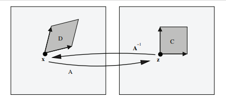
for some $m \times n$ matrix $B$. Note that, by Theorem 1.8.1, Z has expectation vector $\boldsymbol{\mu}$ and covariance matrix $\Sigma=B B^{\top}$. Any random vector of the form (1.23) is said to have a jointly normal or multivariate normal distribution. We write $\mathbf{Z} \sim N(\boldsymbol{\mu}, \Sigma)$. Suppose that $B$ is an invertible $n \times n$ matrix. Then, by (1.19), the density of $\mathbf{Y}=\mathbf{Z}-\boldsymbol{\mu}$ is given by
$$
f_{\mathbf{Y}}(\mathbf{y})=\frac{1}{|B| \sqrt{(2 \pi)^{n}}} \mathrm{e}^{-\frac{1}{2}\left(B^{-1} \mathbf{y}\right)^{\top} B^{-1} \mathbf{y}}=\frac{1}{|B| \sqrt{(2 \pi)^{n}}} \mathrm{e}^{-\frac{1}{2} \mathbf{y}^{\top}\left(B^{-1}\right)^{\top} B^{-1} \mathbf{y}} .
$$
We have $|B|=\sqrt{|\Sigma|}$ and $\left(B^{-1}\right)^{\top} B^{-1}=\left(B^{\top}\right)^{-1} B^{-1}=\left(B B^{\top}\right)^{-1}=\Sigma^{-1}$, so that
$$
f_{\mathbf{Y}}(\mathbf{y})=\frac{1}{\sqrt{(2 \pi)^{n}|\Sigma|}} \mathrm{e}^{-\frac{1}{2} \mathbf{y}^{\top} \Sigma^{-1} \mathbf{y}} .
$$
Because $\mathbf{Z}$ is obtained from $\mathbf{Y}$ by simply adding a constant vector $\boldsymbol{\mu}$, we have $f_{\mathbf{Z}}(\mathbf{z})=f_{\mathbf{Y}}(\mathbf{z}-\boldsymbol{\mu})$, and therefore
$$
f_{\mathbf{Z}}(\mathbf{z})=\frac{1}{\sqrt{(2 \pi)^{n}|\Sigma|}} \mathrm{e}^{-\frac{1}{2}(\mathbf{z}-\boldsymbol{\mu})^{\top} \Sigma^{-1}(\mathbf{z}-\mu)}, \quad \mathbf{z} \in \mathbb{R}^{n} .
$$
Note that this formula is very similar to that of the one-dimensional case.
Conversely, given a covariance matrix $\Sigma=\left(\sigma_{i j}\right)$, there exists a unique lower triangular matrix
$$
B=\left(\begin{array}{cccc}
b_{11} & 0 & \cdots & 0 \
b_{21} & b_{22} & \cdots & 0 \
\vdots & \vdots & & \vdots \
b_{n 1} & b_{n 2} & \cdots & b_{n n}
\end{array}\right)
$$
such that $\Sigma=B B^{\top}$. This matrix can be obtained efficiently via the Cholesky square root method; see Section A.1 of the Appendix.
统计代写|蒙特卡洛方法代写monte carlo method代考|LIMIT THEOREMS
We briefly discuss two of the main results in probability: the law of large numbers and the central limit theorem. Both are associated with sums of independent random variables.
Let $X_{1}, X_{2}, \ldots$ be iid random variables with expectation $\mu$ and variance $\sigma^{2}$. For each $n$, let $S_{n}=X_{1}+\cdots+X_{n}$. Since $X_{1}, X_{2}, \ldots$ are iid, we have $\mathbb{E}\left[S_{n}\right]=n \mathbb{E}\left[X_{1}\right]=$ $n \mu$ and $\operatorname{Var}\left(S_{n}\right)=n \operatorname{Var}\left(X_{1}\right)=n \sigma^{2}$.
The law of large numbers states that $S_{n} / n$ is close to $\mu$ for large $n$. Here is the more precise statement.
Theorem 1.11.1 (Strong Law of Large Numbers) If $X_{1}, \ldots, X_{n}$ are iid with expectation $\mu$, then
$$
\mathbb{P}\left(\lim {n \rightarrow \infty} \frac{S{n}}{n}=\mu\right)=1
$$
The central limit theorem describes the limiting distribution of $S_{n}$ (or $S_{n} / n$ ), and it applies to both continuous and discrete random variables. Loosely, it states that the random sum $S_{n}$ has a distribution that is approximately normal, when $n$ is large. The more precise statement is given next.
Theorem 1.11.2 (Central Limit Theorem) If $X_{1}, \ldots, X_{n}$ are iid with expectation $\mu$ and variance $\sigma^{2}<\infty$, then for all $x \in \mathbb{R}$,
$$
\lim {n \rightarrow \infty} \mathbb{P}\left(\frac{S{n}-n \mu}{\sigma \sqrt{n}} \leqslant x\right)=\Phi(x),
$$
where $\Phi$ is the cdf of the standard normal distribution.
In other words, $S_{n}$ has a distribution that is approximately normal, with expectation $n \mu$ and variance $n \sigma^{2}$. To see the central limit theorem in action, consider Figure 1.2. The left part shows the pdfs of $S_{1}, \ldots, S_{4}$ for the case where the $\left{X_{i}\right}$ have a $U[0,1]$ distribution. The right part shows the same for the $\operatorname{Exp}(1)$ distribution. We clearly see convergence to a bell-shaped curve, characteristic of the normal distribution.
统计代写|蒙特卡洛方法代写monte carlo method代考|POISSON PROCESSES
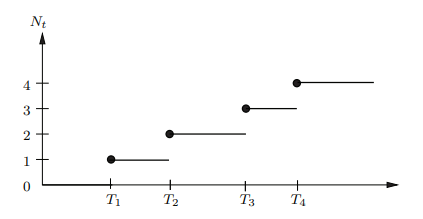
The Poisson process is used to model certain kinds of arrivals or patterns. Imagine, for example, a telescope that can detect individual photons from a faraway galaxy. The photons arrive at random times $T_{1}, T_{2}, \ldots .$ Let $N_{t}$ denote the number of arrivals in the time interval $[0, t]$, that is, $N_{t}=\sup \left{k: T_{k} \leqslant t\right}$. Note that the number of arrivals in an interval $I=(a, b]$ is given by $N_{b}-N_{a}$. We will also denote it by $N(a, b]$. A sample path of the arrival counting process $\left{N_{t}, t \geqslant 0\right}$ is given in Figure 1.3.
For this particular arrival process, one would assume that the number of arrivals in an interval $(a, b)$ is independent of the number of arrivals in interval $(c, d)$ when the two intervals do not intersect. Such considerations lead to the following definition:
Definition 1.12.1 (Poisson Process) An arrival counting process $N=\left{N_{t}\right}$ is called a Poisson process with rate $\lambda>0$ if
(a) The numbers of points in nonoverlapping intervals are independent.
(b) The number of points in interval $I$ has a Poisson distribution with mean $\lambda \times \operatorname{length}(I)$.
monte carlo method代写
统计代写|蒙特卡洛方法代写monte carlo method代考|JOINTLY NORMAL RANDOM VARIABLES
将正态分布的随机变量视为标准正态的简单变换是有帮助的——也就是说,ñ(0,1)-分布式——随机变量。特别是,让X∼ñ(0,1). 然后X有密度FX由
FX(X)=12圆周率和−X22.
现在考虑转换从=μ+σX. 然后,由 (1.15),从有密度
F从(和)=12圆周率σ2和−(和−μ)22σ2.
换句话说,从∼ñ(μ,σ2). 我们也可以这样表述:如果从∼ñ(μ,σ2), 然后(从−μ)/σ∼ñ(0,1). 这个过程称为标准化。
我们现在将其推广到n方面。让X1,…,Xn是独立的标准正态随机变量。联合pdfX=(X1,…,Xn)⊤是(谁)给的
FX(X)=(2圆周率)−n/2和−12X⊤X,X∈Rn.
考虑仿射变换(即线性变换加常数向量)
从=μ+乙X
对于一些米×n矩阵乙. 请注意,根据定理 1.8.1,Z 具有期望向量μ和协方差矩阵Σ=乙乙⊤. 任何形式为 (1.23) 的随机向量都被称为具有联合正态分布或多元正态分布。我们写从∼ñ(μ,Σ). 假设乙是可逆的n×n矩阵。然后,由(1.19),密度是=从−μ是(谁)给的
F是(是)=1|乙|(2圆周率)n和−12(乙−1是)⊤乙−1是=1|乙|(2圆周率)n和−12是⊤(乙−1)⊤乙−1是.
我们有|乙|=|Σ|和(乙−1)⊤乙−1=(乙⊤)−1乙−1=(乙乙⊤)−1=Σ−1, 以便
F是(是)=1(2圆周率)n|Σ|和−12是⊤Σ−1是.
因为从是从是通过简单地添加一个常数向量μ, 我们有F从(和)=F是(和−μ),因此
F从(和)=1(2圆周率)n|Σ|和−12(和−μ)⊤Σ−1(和−μ),和∈Rn.
请注意,此公式与一维情况的公式非常相似。
相反,给定一个协方差矩阵Σ=(σ一世j), 存在唯一的下三角矩阵
乙=(b110⋯0 b21b22⋯0 ⋮⋮⋮ bn1bn2⋯bnn)
这样Σ=乙乙⊤. 该矩阵可以通过 Cholesky 平方根方法有效地获得;见附录 A.1 节。
统计代写|蒙特卡洛方法代写monte carlo method代考|LIMIT THEOREMS
我们简要讨论概率的两个主要结果:大数定律和中心极限定理。两者都与独立随机变量的总和有关。
让X1,X2,…是具有期望的独立同分布随机变量μ和方差σ2. 对于每个n, 让小号n=X1+⋯+Xn. 自从X1,X2,…是 iid,我们有和[小号n]=n和[X1]= nμ和曾是(小号n)=n曾是(X1)=nσ2.
大数定律指出小号n/n接近μ对于大n. 这是更准确的说法。
定理 1.11.1(大数强定律)如果X1,…,Xn充满期待μ, 然后
磷(林n→∞小号nn=μ)=1
中心极限定理描述了小号n(或者小号n/n),它适用于连续和离散的随机变量。松散地,它指出随机和小号n具有近似正态分布,当n很大。接下来给出更准确的陈述。
定理 1.11.2(中心极限定理)如果X1,…,Xn充满期待μ和方差σ2<∞, 那么对于所有X∈R,
林n→∞磷(小号n−nμσn⩽X)=披(X),
在哪里披是标准正态分布的 cdf。
换句话说,小号n具有近似正态分布,具有期望nμ和方差nσ2. 要查看实际的中心极限定理,请考虑图 1.2。左边部分显示了pdf小号1,…,小号4对于这种情况\left{X_{i}\right}\left{X_{i}\right}有一个在[0,1]分配。右侧部分显示相同的经验(1)分配。我们清楚地看到收敛到钟形曲线,这是正态分布的特征。
统计代写|蒙特卡洛方法代写monte carlo method代考|POISSON PROCESSES
泊松过程用于对某些类型的到达或模式进行建模。例如,想象一个可以探测到来自遥远星系的单个光子的望远镜。光子随机到达吨1,吨2,….让ñ吨表示时间间隔内的到达次数[0,吨], 那是,N_{t}=\sup \left{k: T_{k} \leqslant t\right}N_{t}=\sup \left{k: T_{k} \leqslant t\right}. 注意一个区间内的到达次数一世=(一种,b]是(谁)给的ñb−ñ一种. 我们也将其表示为ñ(一种,b]. 到达计数过程的示例路径\left{N_{t}, t \geqslant 0\right}\left{N_{t}, t \geqslant 0\right}如图 1.3 所示。
对于这个特定的到达过程,可以假设一个区间内的到达次数(一种,b)与区间内的到达次数无关(C,d)当两个区间不相交时。这些考虑导致了以下定义:
定义 1.12.1(泊松过程)到达计数过程N=\left{N_{t}\right}N=\left{N_{t}\right}称为具有速率的泊松过程λ>0如果
(a) 非重叠区间中的点数是独立的。
(b) 区间点数一世具有均值的泊松分布λ×长度(一世).

统计代写请认准statistics-lab™. statistics-lab™为您的留学生涯保驾护航。
金融工程代写
金融工程是使用数学技术来解决金融问题。金融工程使用计算机科学、统计学、经济学和应用数学领域的工具和知识来解决当前的金融问题,以及设计新的和创新的金融产品。
非参数统计代写
非参数统计指的是一种统计方法,其中不假设数据来自于由少数参数决定的规定模型;这种模型的例子包括正态分布模型和线性回归模型。
广义线性模型代考
广义线性模型(GLM)归属统计学领域,是一种应用灵活的线性回归模型。该模型允许因变量的偏差分布有除了正态分布之外的其它分布。
术语 广义线性模型(GLM)通常是指给定连续和/或分类预测因素的连续响应变量的常规线性回归模型。它包括多元线性回归,以及方差分析和方差分析(仅含固定效应)。
有限元方法代写
有限元方法(FEM)是一种流行的方法,用于数值解决工程和数学建模中出现的微分方程。典型的问题领域包括结构分析、传热、流体流动、质量运输和电磁势等传统领域。
有限元是一种通用的数值方法,用于解决两个或三个空间变量的偏微分方程(即一些边界值问题)。为了解决一个问题,有限元将一个大系统细分为更小、更简单的部分,称为有限元。这是通过在空间维度上的特定空间离散化来实现的,它是通过构建对象的网格来实现的:用于求解的数值域,它有有限数量的点。边界值问题的有限元方法表述最终导致一个代数方程组。该方法在域上对未知函数进行逼近。[1] 然后将模拟这些有限元的简单方程组合成一个更大的方程系统,以模拟整个问题。然后,有限元通过变化微积分使相关的误差函数最小化来逼近一个解决方案。
tatistics-lab作为专业的留学生服务机构,多年来已为美国、英国、加拿大、澳洲等留学热门地的学生提供专业的学术服务,包括但不限于Essay代写,Assignment代写,Dissertation代写,Report代写,小组作业代写,Proposal代写,Paper代写,Presentation代写,计算机作业代写,论文修改和润色,网课代做,exam代考等等。写作范围涵盖高中,本科,研究生等海外留学全阶段,辐射金融,经济学,会计学,审计学,管理学等全球99%专业科目。写作团队既有专业英语母语作者,也有海外名校硕博留学生,每位写作老师都拥有过硬的语言能力,专业的学科背景和学术写作经验。我们承诺100%原创,100%专业,100%准时,100%满意。
随机分析代写
随机微积分是数学的一个分支,对随机过程进行操作。它允许为随机过程的积分定义一个关于随机过程的一致的积分理论。这个领域是由日本数学家伊藤清在第二次世界大战期间创建并开始的。
时间序列分析代写
随机过程,是依赖于参数的一组随机变量的全体,参数通常是时间。 随机变量是随机现象的数量表现,其时间序列是一组按照时间发生先后顺序进行排列的数据点序列。通常一组时间序列的时间间隔为一恒定值(如1秒,5分钟,12小时,7天,1年),因此时间序列可以作为离散时间数据进行分析处理。研究时间序列数据的意义在于现实中,往往需要研究某个事物其随时间发展变化的规律。这就需要通过研究该事物过去发展的历史记录,以得到其自身发展的规律。
回归分析代写
多元回归分析渐进(Multiple Regression Analysis Asymptotics)属于计量经济学领域,主要是一种数学上的统计分析方法,可以分析复杂情况下各影响因素的数学关系,在自然科学、社会和经济学等多个领域内应用广泛。
MATLAB代写
MATLAB 是一种用于技术计算的高性能语言。它将计算、可视化和编程集成在一个易于使用的环境中,其中问题和解决方案以熟悉的数学符号表示。典型用途包括:数学和计算算法开发建模、仿真和原型制作数据分析、探索和可视化科学和工程图形应用程序开发,包括图形用户界面构建MATLAB 是一个交互式系统,其基本数据元素是一个不需要维度的数组。这使您可以解决许多技术计算问题,尤其是那些具有矩阵和向量公式的问题,而只需用 C 或 Fortran 等标量非交互式语言编写程序所需的时间的一小部分。MATLAB 名称代表矩阵实验室。MATLAB 最初的编写目的是提供对由 LINPACK 和 EISPACK 项目开发的矩阵软件的轻松访问,这两个项目共同代表了矩阵计算软件的最新技术。MATLAB 经过多年的发展,得到了许多用户的投入。在大学环境中,它是数学、工程和科学入门和高级课程的标准教学工具。在工业领域,MATLAB 是高效研究、开发和分析的首选工具。MATLAB 具有一系列称为工具箱的特定于应用程序的解决方案。对于大多数 MATLAB 用户来说非常重要,工具箱允许您学习和应用专业技术。工具箱是 MATLAB 函数(M 文件)的综合集合,可扩展 MATLAB 环境以解决特定类别的问题。可用工具箱的领域包括信号处理、控制系统、神经网络、模糊逻辑、小波、仿真等。