月度归档: 2022 年 12 月

数学代写|勒贝格积分代写Lebesgue Integration代考|Math720

如果你也在 怎样代写勒贝格积分Lebesgue Integration这个学科遇到相关的难题,请随时右上角联系我们的24/7代写客服。

勒贝格积分一词既可以指勒贝格积分提出的关于函数相对于一般度量的积分的一般理论,也可以指定义在实线子域上的函数相对于勒贝格积分度量的积分的具体情形。

statistics-lab™ 为您的留学生涯保驾护航 在代写勒贝格积分Lebesgue Integration方面已经树立了自己的口碑, 保证靠谱, 高质且原创的统计Statistics代写服务。我们的专家在代写勒贝格积分Lebesgue Integration代写方面经验极为丰富,各种代写勒贝格积分Lebesgue Integration相关的作业也就用不着说。

我们提供的勒贝格积分Lebesgue Integration及其相关学科的代写,服务范围广, 其中包括但不限于:

  • Statistical Inference 统计推断
  • Statistical Computing 统计计算
  • Advanced Probability Theory 高等概率论
  • Advanced Mathematical Statistics 高等数理统计学
  • (Generalized) Linear Models 广义线性模型
  • Statistical Machine Learning 统计机器学习
  • Longitudinal Data Analysis 纵向数据分析
  • Foundations of Data Science 数据科学基础
数学代写|勒贝格积分代写Lebesgue Integration代考|Math720

数学代写|勒贝格积分代写Lebesgue Integration代考|Continuity and Differentiability

The fourth big question asks for the relationship between continuity and differentiability. We know that a function that is differentiable at a given value of $x$ must also be continuous at that value, and it is clear that the converse does not hold. The function $f(x)=|x|$ is continuous but not differentiable at $x=0$. But how nondifferentiable can a continuous function be?

Throughout the first half of the nineteenth century, it was generally believed that a continuous function would be differentiable at most points. ${ }^4$ Mathematicians recognized that a function might have finitely many values at which it failed to have a derivative. There might even be a sparse infinite set of points at which a continuous function was not differentiable, but the mathematical community was honestly surprised when, in 1875 , Gaston Darboux and Paul du-Bois Reymond ${ }^5$ published examples of continuous functions that are not differentiable at any value.
The question then shifted to what additional assumptions beyond continuity would ensure differentiability. Monotonicity was a natural candidate. Weierstrass constructed a strictly increasing continuous function that is not differentiable at any algebraic number, that is to say, at any number that is the root of a polynomial with rational coefficients. It is not differentiable at $1 / 2$ or $\sqrt{2}$ or $\sqrt[3]{5}-2 \sqrt[21]{35}$. Weierstrass’s function is differentiable at $\pi$. Can we find a continuous, increasing function that is not differentiable at any value? The surprising answer is No. In fact, in a sense that later will be made precise, a continuous, monotonic function is differentiable at “most” values of $x$. There are very important subtleties lurking behind this fourth question.

数学代写|勒贝格积分代写Lebesgue Integration代考|Term-by-term Integration

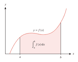
Returning to Fourier series, we saw that the heuristic justification relied on interchanging summation and integration, integrating an infinite series of functions by integrating each summand. This works for finite summations. It is not hard to find infinite series for which term-by-term integration leads to a divergent series or, even worse, a series that converges to the wrong value.

Weierstrass had shown that if the series converges uniformly, then term-by-term integration is valid. The problem with this result is that the most interesting series, especially Fourier series, often do not converge uniformly and yet term-by-term integration is valid. Uniform convergence is sufficient, but it is very far from necessary. As we shall see, finding useful conditions under which term-by-term integration is valid is very difficult so long as we cling to the Riemann integral. As Lebesgue would show in the opening years of the twentieth century, his definition of the integral yields a simple, elegant solution, the Lebesgue dominated convergence theorem.

1.1.1. Find the Fourier expansions for $f_1(x)=x$ and $f_2(x)=x^2$ over $[-\pi, \pi]$.
1.1.2. For the functions $f_1$ and $f_2$ defined in Exercise 1.1.1, differentiate each summand in the Fourier series for $f_2$. Do you get the summands in the Fourier series for $2 f_1$ ? Differentiate each summand in the Fourier series for $f_1$. Do you get the summand in the Fourier series for $f_1^{\prime}(x)$ ?
1.1.3. Using the Fourier series expansion for $x^2$ (Exercise 1.1.1) evaluated at $x=\pi$, show that
$$
\sum_{n=1}^{\infty} \frac{1}{n^2}=\frac{\pi^2}{6} .
$$
1.1.4. Show that if $k$ is an integer $\geq 1$, then
$$
\int_{-\pi}^\pi \cos (k x) d x=\int_{-\pi}^\pi \sin (k x) d x=0 .
$$

数学代写|勒贝格积分代写Lebesgue Integration代考|Math720

勒贝格积分代考

数学代写|勒贝格积分代写Lebesgue Integration代考|Continuity and Differentiability

第四个大问题是连续性和可微性之间的关系。我们知道在给定的值下可微分的函数 $x$ 也必须在该值处连 续,很明显,反之亦然。功能 $f(x)=|x|$ 是连续的但在 $x=0$. 但是连续函数的不可微性如何呢?
在整个 19 世纪上半叶,人们普遍认为连续函数在大多数点上都是可微的。 4 数学家们认识到,一个函数 可能有有限多个值,在这些值处它没有导数。甚至可能存在连续函数不可微的稀疏无限点集,但当 1875 年 Gaston Darboux 和 Paul du-Bois Reymond 时,数学界真的感到惊讶 ${ }^5$ 已发布的在任何值下均不可微 的连续函数示例。
然后问题转移到除了连续性之外还有哪些额外的假设可以确保可微性。单调性是一个自然的候选者。 Weierstrass 构造了一个严格递增的连续函数,该函数在任何代数数处不可微,也就是说,在作为具有有 理系数的多项式的根的任何数处不可微。它不可微 $1 / 2$ 要么 $\sqrt{2}$ 要么 $\sqrt[3]{5}-2 \sqrt[21]{35}$. Weierstrass 的函数在 $\pi$. 我们能否找到一个在任何值下都不可微的连续增函数? 令人惊讶的答案是否定的。事实上,从某种意 义上说,以后会变得精确,一个连续的、单调的函数在”大多数”值处是可微的。 $x$. 第四个问题背后隐藏着 非常重要的微妙之处。

数学代写|勒贝格积分代写Lebesgue Integration代考|Term-by-term Integration

回到傅里叶级数,我们看到启发式论证依赖于求和和积分的交替,通过积分每个被加数来积分无限系列 的函数。这适用于有限求和。不难发现无限级数,其中逐项积分导致发散级数,或者更糟糕的是,级数 收敛到错误的值。

Weierstrass 已经表明,如果级数一致收敛,则逐项积分是有效的。这个结果的问题在于,最有趣的级 数,尤其是傅立叶级数,通常不会一致收敛,但逐项积分是有效的。均匀收敛就足够了,但远非必要。 正如我们将要看到的,只要我们坚持黎曼积分,就很难找到使逐项积分有效的有用条件。正如勒贝格在 20 世纪初所表明的那样,他对积分的定义产生了一个简单、优雅的解决方案,即勒贝格支配的收敛定 理。
1.1.1. 求傅立叶展开式 $f_1(x)=x$ 和 $f_2(x)=x^2$ 超过 $[-\pi, \pi]$.
1.1.2. 对于函数 $f_1$ 和 $f_2$ 在练习 1.1.1 中定义,区分傅立叶级数中的每个被加数 $f_2$. 你得到傅立叶级数中的 被加数了吗 $2 f_1$ ? 区分傅里叶级数中的每个被加数 $f_1$. 你得到傅立叶级数中的被加数了吗 $f_1^{\prime}(x)$ ?
1.1.3. 使用傅里叶级数展开 $x^2$ (练习 1.1.1) 评估于 $x=\pi$ , 显示
$$
\sum_{n=1}^{\infty} \frac{1}{n^2}=\frac{\pi^2}{6}
$$
1.1.4. 证明如果 $k$ 是一个整数 $\geq 1$ , 然后
$$
\int_{-\pi}^\pi \cos (k x) d x=\int_{-\pi}^\pi \sin (k x) d x=0
$$

数学代写|勒贝格积分代写Lebesgue Integration代考 请认准statistics-lab™

统计代写请认准statistics-lab™. statistics-lab™为您的留学生涯保驾护航。

金融工程代写

金融工程是使用数学技术来解决金融问题。金融工程使用计算机科学、统计学、经济学和应用数学领域的工具和知识来解决当前的金融问题,以及设计新的和创新的金融产品。

非参数统计代写

非参数统计指的是一种统计方法,其中不假设数据来自于由少数参数决定的规定模型;这种模型的例子包括正态分布模型和线性回归模型。

广义线性模型代考

广义线性模型(GLM)归属统计学领域,是一种应用灵活的线性回归模型。该模型允许因变量的偏差分布有除了正态分布之外的其它分布。

术语 广义线性模型(GLM)通常是指给定连续和/或分类预测因素的连续响应变量的常规线性回归模型。它包括多元线性回归,以及方差分析和方差分析(仅含固定效应)。

有限元方法代写

有限元方法(FEM)是一种流行的方法,用于数值解决工程和数学建模中出现的微分方程。典型的问题领域包括结构分析、传热、流体流动、质量运输和电磁势等传统领域。

有限元是一种通用的数值方法,用于解决两个或三个空间变量的偏微分方程(即一些边界值问题)。为了解决一个问题,有限元将一个大系统细分为更小、更简单的部分,称为有限元。这是通过在空间维度上的特定空间离散化来实现的,它是通过构建对象的网格来实现的:用于求解的数值域,它有有限数量的点。边界值问题的有限元方法表述最终导致一个代数方程组。该方法在域上对未知函数进行逼近。[1] 然后将模拟这些有限元的简单方程组合成一个更大的方程系统,以模拟整个问题。然后,有限元通过变化微积分使相关的误差函数最小化来逼近一个解决方案。

tatistics-lab作为专业的留学生服务机构,多年来已为美国、英国、加拿大、澳洲等留学热门地的学生提供专业的学术服务,包括但不限于Essay代写,Assignment代写,Dissertation代写,Report代写,小组作业代写,Proposal代写,Paper代写,Presentation代写,计算机作业代写,论文修改和润色,网课代做,exam代考等等。写作范围涵盖高中,本科,研究生等海外留学全阶段,辐射金融,经济学,会计学,审计学,管理学等全球99%专业科目。写作团队既有专业英语母语作者,也有海外名校硕博留学生,每位写作老师都拥有过硬的语言能力,专业的学科背景和学术写作经验。我们承诺100%原创,100%专业,100%准时,100%满意。

随机分析代写


随机微积分是数学的一个分支,对随机过程进行操作。它允许为随机过程的积分定义一个关于随机过程的一致的积分理论。这个领域是由日本数学家伊藤清在第二次世界大战期间创建并开始的。

时间序列分析代写

随机过程,是依赖于参数的一组随机变量的全体,参数通常是时间。 随机变量是随机现象的数量表现,其时间序列是一组按照时间发生先后顺序进行排列的数据点序列。通常一组时间序列的时间间隔为一恒定值(如1秒,5分钟,12小时,7天,1年),因此时间序列可以作为离散时间数据进行分析处理。研究时间序列数据的意义在于现实中,往往需要研究某个事物其随时间发展变化的规律。这就需要通过研究该事物过去发展的历史记录,以得到其自身发展的规律。

回归分析代写

多元回归分析渐进(Multiple Regression Analysis Asymptotics)属于计量经济学领域,主要是一种数学上的统计分析方法,可以分析复杂情况下各影响因素的数学关系,在自然科学、社会和经济学等多个领域内应用广泛。

MATLAB代写

MATLAB 是一种用于技术计算的高性能语言。它将计算、可视化和编程集成在一个易于使用的环境中,其中问题和解决方案以熟悉的数学符号表示。典型用途包括:数学和计算算法开发建模、仿真和原型制作数据分析、探索和可视化科学和工程图形应用程序开发,包括图形用户界面构建MATLAB 是一个交互式系统,其基本数据元素是一个不需要维度的数组。这使您可以解决许多技术计算问题,尤其是那些具有矩阵和向量公式的问题,而只需用 C 或 Fortran 等标量非交互式语言编写程序所需的时间的一小部分。MATLAB 名称代表矩阵实验室。MATLAB 最初的编写目的是提供对由 LINPACK 和 EISPACK 项目开发的矩阵软件的轻松访问,这两个项目共同代表了矩阵计算软件的最新技术。MATLAB 经过多年的发展,得到了许多用户的投入。在大学环境中,它是数学、工程和科学入门和高级课程的标准教学工具。在工业领域,MATLAB 是高效研究、开发和分析的首选工具。MATLAB 具有一系列称为工具箱的特定于应用程序的解决方案。对于大多数 MATLAB 用户来说非常重要,工具箱允许您学习应用专业技术。工具箱是 MATLAB 函数(M 文件)的综合集合,可扩展 MATLAB 环境以解决特定类别的问题。可用工具箱的领域包括信号处理、控制系统、神经网络、模糊逻辑、小波、仿真等。

R语言代写问卷设计与分析代写
PYTHON代写回归分析与线性模型代写
MATLAB代写方差分析与试验设计代写
STATA代写机器学习/统计学习代写
SPSS代写计量经济学代写
EVIEWS代写时间序列分析代写
EXCEL代写深度学习代写
SQL代写各种数据建模与可视化代写

数学代写|勒贝格积分代写Lebesgue Integration代考|MATH6210

如果你也在 怎样代写勒贝格积分Lebesgue Integration这个学科遇到相关的难题,请随时右上角联系我们的24/7代写客服。

勒贝格积分一词既可以指勒贝格积分提出的关于函数相对于一般度量的积分的一般理论,也可以指定义在实线子域上的函数相对于勒贝格积分度量的积分的具体情形。

statistics-lab™ 为您的留学生涯保驾护航 在代写勒贝格积分Lebesgue Integration方面已经树立了自己的口碑, 保证靠谱, 高质且原创的统计Statistics代写服务。我们的专家在代写勒贝格积分Lebesgue Integration代写方面经验极为丰富,各种代写勒贝格积分Lebesgue Integration相关的作业也就用不着说。

我们提供的勒贝格积分Lebesgue Integration及其相关学科的代写,服务范围广, 其中包括但不限于:

  • Statistical Inference 统计推断
  • Statistical Computing 统计计算
  • Advanced Probability Theory 高等概率论
  • Advanced Mathematical Statistics 高等数理统计学
  • (Generalized) Linear Models 广义线性模型
  • Statistical Machine Learning 统计机器学习
  • Longitudinal Data Analysis 纵向数据分析
  • Foundations of Data Science 数据科学基础
数学代写|勒贝格积分代写Lebesgue Integration代考|MATH6210

数学代写|勒贝格积分代写Lebesgue Integration代考|The Fundamental Theorem of Calculus

The fundamental theorem of calculus is, in essence, simply a statement of the equivalence of the two means of understanding integration, as the inverse process of differentiation and as a limit of sums of products. The precise theorems to which this designation refers today arise from the assumption that integration is defined as a limiting process. They then clarify the precise relationship between integration and differentiation. The actual statements that we shall use are given by the following theorems.

Theorem 1.1 (FTC, evaluation). If $f$ is the derivative of $F$ at every point on $[a, b]$, then under suitable hypotheses we have that
$$
\int_a^b f(t) d t=F(b)-F(a) .
$$
Theorem $1.2$ (FTC, antiderivative). If $f$ is integrable on the interval $[a, b]$, then under suitable hypotheses we have that
$$
\frac{d}{d x} \int_a^x f(t) d t=f(x) .
$$
The first of these theorems tells us how we can use any antiderivative to obtain a simple evaluation of a definite integral. The second shows that the definite integral can be used to create an antiderivative, the definite integral of $f$ from $a$ to $x$ is a function of $x$ whose derivative is $f$. Both of these statements would be meaningless if we had defined the integral as the antiderivative. Their meaning and importance comes from the assumption that $\int_a^b f(t) d t$ is defined as a limit of summations.
In both cases, I have not specified the hypotheses under which these theorems hold. There are two reasons for this. One is that much of the interesting story that is to be told about the creation of analysis in the late nineteenth century revolves around finding necessary and sufficient conditions under which the conclusions hold. When working with Riemann’s definition of the integal, the answer is complicated. The second reason is that the hypotheses that are needed depend on the way we choose to define the integral. For Lebesgue’s definition, the hypotheses are quite different.

数学代写|勒贝格积分代写Lebesgue Integration代考|A Brief History of Theorems 1.1 and 1.22

The earliest reference to Theorem $1.1$ of which I am aware is Siméon Denis Poisson’s 1820 Suite du Mémoire sur les Intégrales Définies. There he refers to it as “the fundamental proposition of the theory of definite integrals.” Poisson’s work is worth some digression because it illustrates the importance of how we define the definite integral and the difficulties encountered when it is defined as the difference of the values of an antiderivative at the endpoints.

Siméon Denis Poisson (1781-1840) studied and then taught at the École Polytechnique. He succeeded to Fourier’s professorship in mathematics when Fourier departed for Grenoble to become prefect of the department of Isère. It was Poisson who wrote up the rejection of Fourier’s Theory of the Propoagation of Heat in Solid Bodies in 1808. When, in 1815, Poisson published his own article on the flow of heat, Fourier pointed out its many flaws and the extent to which Poisson had rediscovered Fourier’s own work.

Poisson, as a colleague of Cauchy at the École Polytechnique, almost certainly was aware of Cauchy’s definition of the definite integral even though Cauchy had not yet published it. But the relationship between Poisson and Cauchy was far from amicable, and it would have been surprising had Poisson chosen to embrace his colleague’s approach. Poisson defines the definite integral as the difference of the values of the antiderivative. It would seem there is nothing to prove. What Poisson does prove is that if $F$ has a Taylor series expansion and $F^{\prime}=f$, then
$$
F(b)-F(a)=\lim {n \rightarrow \infty} \sum{j=1}^n t f(a+(j-1) t), \quad \text { where } t=\frac{b-a}{n} .
$$
Poisson begins with the observation that for $1 \leq j \leq n$ and $t=(b-a) / n$, there is a $k \geq 1$ and a collection of functions $R_j$ such that
$$
F(a+j t)=F(a+(j-1) t)+t f(a+(j-1) t)+t^{1+k} R_j(t),
$$
and therefore
$$
\begin{aligned}
F(b)-F(a) & =\sum_{j=1}^n[F(a+j t)-F(a+(j-1) t)] \
& =\sum_{j=1}^n t f(a+(j-1) t)+t^{1+k} \sum_{j=1}^n R_j(t) .
\end{aligned}
$$

数学代写|勒贝格积分代写Lebesgue Integration代考|MATH6210

勒贝格积分代考

数学代写|勒贝格积分代写Lebesgue Integration代考|The Fundamental Theorem of Calculus

微积分的基本定理本质上只是对理解积分的两种方法的等价性的陈述,即微分的逆过程和乘积和的极 限。今天这个名称所指的精确定理源于积分被定义为限制过程的假设。然后他们阐明了整合和分化之间 的确切关系。我们将使用的实际陈述由以下定理给出。
定理 $1.1$ (FTC,评估) 。如果 $f$ 是导数 $F$ 在每一点上 $[a, b]$, 然后在适当的假设下我们有
$$
\int_a^b f(t) d t=F(b)-F(a)
$$
定理1.2 (FTC,反衍生) 。如果 $f$ 在区间上可积 $[a, b]$, 然后在适当的假设下我们有
$$
\frac{d}{d x} \int_a^x f(t) d t=f(x)
$$
这些定理中的第一个告诉我们如何使用任何反导数来获得定积分的简单计算。第二个表明定积分可用于 创建反导数,即定积分 $f$ 从 $a$ 到 $x$ 是一个函数 $x$ 它的导数是 $f$. 如果我们将积分定义为反导数,那么这两个陈 述将毫无意义。它们的意义和重要性来自以下假设 $\int_a^b f(t) d t$ 被定义为求和的极限。
在这两种情况下,我都没有具体说明这些定理成立的假设。有两个原因。其中之一是关于 19 世纪后期分 析的创建的许多有趣故事都围绕着寻找结论成立的必要和充分条件。在使用黎曼的积分定义时,答案很 复杂。第二个原因是所需的假设取决于我们选择定义积分的方式。对于勒贝格的定义,假设是完全不同 的。

数学代写|勒贝格积分代写Lebesgue Integration代考|A Brief History of Theorems 1.1 and 1.22

最早引用定理1.1其中我知道的是 Siméon Denis Poisson 的 1820 Suite du Mémoire sur les Intégrales Définies。他在那里将其称为 “定积分理论的基本命题”。泊松的工作值得一些题外话,因为它说明了我们 如何定义定积分的重要性,以及将其定义为反导数在端点处的值之差时遇到的困难。

Siméon Denis Poisson (1781-1840) 在巴黎综合理工学院学习并任教。当傅立叶前往格勒诺布尔成为 伊泽尔省省长时,他继承了傅立叶的数学教授职位。正是泊松在 1808 年写下了拒绝傅立叶的固体热传播 理论的文章。在 1815 年,泊松发表了他自己关于热流的文章时,傅立叶指出了它的许多缺陷以及泊松在 多大程度上重新发现了傅里叶自己的工作。
泊松作为柯西在巴黎综合理工学院的同事,几乎可以肯定知道柯西对定积分的定义,尽管柯西尚末发表 它。但泊松和柯西之间的关系远非友好,如果泊松选择接受他同事的方法,那将是令人惊讶的。泊松将 定积分定义为反导数值的差值。似乎没有什么可以证明的。泊松证明的是,如果 $F$ 有泰勒级数展开和 $F^{\prime}=f ,$ 然后
$$
F(b)-F(a)=\lim n \rightarrow \infty \sum j=1^n t f(a+(j-1) t), \quad \text { where } t=\frac{b-a}{n} .
$$
泊松从观察开始,对于 $1 \leq j \leq n$ 和 $t=(b-a) / n$ ,有一个 $k \geq 1$ 和一系列功能 $R_j$ 这样
$$
F(a+j t)=F(a+(j-1) t)+t f(a+(j-1) t)+t^{1+k} R_j(t),
$$
因此
$$
F(b)-F(a)=\sum_{j=1}^n[F(a+j t)-F(a+(j-1) t)] \quad=\sum_{j=1}^n t f(a+(j-1) t)+t^{1+k} \sum_{j=1}^n R_j(t)
$$

数学代写|勒贝格积分代写Lebesgue Integration代考 请认准statistics-lab™

统计代写请认准statistics-lab™. statistics-lab™为您的留学生涯保驾护航。

金融工程代写

金融工程是使用数学技术来解决金融问题。金融工程使用计算机科学、统计学、经济学和应用数学领域的工具和知识来解决当前的金融问题,以及设计新的和创新的金融产品。

非参数统计代写

非参数统计指的是一种统计方法,其中不假设数据来自于由少数参数决定的规定模型;这种模型的例子包括正态分布模型和线性回归模型。

广义线性模型代考

广义线性模型(GLM)归属统计学领域,是一种应用灵活的线性回归模型。该模型允许因变量的偏差分布有除了正态分布之外的其它分布。

术语 广义线性模型(GLM)通常是指给定连续和/或分类预测因素的连续响应变量的常规线性回归模型。它包括多元线性回归,以及方差分析和方差分析(仅含固定效应)。

有限元方法代写

有限元方法(FEM)是一种流行的方法,用于数值解决工程和数学建模中出现的微分方程。典型的问题领域包括结构分析、传热、流体流动、质量运输和电磁势等传统领域。

有限元是一种通用的数值方法,用于解决两个或三个空间变量的偏微分方程(即一些边界值问题)。为了解决一个问题,有限元将一个大系统细分为更小、更简单的部分,称为有限元。这是通过在空间维度上的特定空间离散化来实现的,它是通过构建对象的网格来实现的:用于求解的数值域,它有有限数量的点。边界值问题的有限元方法表述最终导致一个代数方程组。该方法在域上对未知函数进行逼近。[1] 然后将模拟这些有限元的简单方程组合成一个更大的方程系统,以模拟整个问题。然后,有限元通过变化微积分使相关的误差函数最小化来逼近一个解决方案。

tatistics-lab作为专业的留学生服务机构,多年来已为美国、英国、加拿大、澳洲等留学热门地的学生提供专业的学术服务,包括但不限于Essay代写,Assignment代写,Dissertation代写,Report代写,小组作业代写,Proposal代写,Paper代写,Presentation代写,计算机作业代写,论文修改和润色,网课代做,exam代考等等。写作范围涵盖高中,本科,研究生等海外留学全阶段,辐射金融,经济学,会计学,审计学,管理学等全球99%专业科目。写作团队既有专业英语母语作者,也有海外名校硕博留学生,每位写作老师都拥有过硬的语言能力,专业的学科背景和学术写作经验。我们承诺100%原创,100%专业,100%准时,100%满意。

随机分析代写


随机微积分是数学的一个分支,对随机过程进行操作。它允许为随机过程的积分定义一个关于随机过程的一致的积分理论。这个领域是由日本数学家伊藤清在第二次世界大战期间创建并开始的。

时间序列分析代写

随机过程,是依赖于参数的一组随机变量的全体,参数通常是时间。 随机变量是随机现象的数量表现,其时间序列是一组按照时间发生先后顺序进行排列的数据点序列。通常一组时间序列的时间间隔为一恒定值(如1秒,5分钟,12小时,7天,1年),因此时间序列可以作为离散时间数据进行分析处理。研究时间序列数据的意义在于现实中,往往需要研究某个事物其随时间发展变化的规律。这就需要通过研究该事物过去发展的历史记录,以得到其自身发展的规律。

回归分析代写

多元回归分析渐进(Multiple Regression Analysis Asymptotics)属于计量经济学领域,主要是一种数学上的统计分析方法,可以分析复杂情况下各影响因素的数学关系,在自然科学、社会和经济学等多个领域内应用广泛。

MATLAB代写

MATLAB 是一种用于技术计算的高性能语言。它将计算、可视化和编程集成在一个易于使用的环境中,其中问题和解决方案以熟悉的数学符号表示。典型用途包括:数学和计算算法开发建模、仿真和原型制作数据分析、探索和可视化科学和工程图形应用程序开发,包括图形用户界面构建MATLAB 是一个交互式系统,其基本数据元素是一个不需要维度的数组。这使您可以解决许多技术计算问题,尤其是那些具有矩阵和向量公式的问题,而只需用 C 或 Fortran 等标量非交互式语言编写程序所需的时间的一小部分。MATLAB 名称代表矩阵实验室。MATLAB 最初的编写目的是提供对由 LINPACK 和 EISPACK 项目开发的矩阵软件的轻松访问,这两个项目共同代表了矩阵计算软件的最新技术。MATLAB 经过多年的发展,得到了许多用户的投入。在大学环境中,它是数学、工程和科学入门和高级课程的标准教学工具。在工业领域,MATLAB 是高效研究、开发和分析的首选工具。MATLAB 具有一系列称为工具箱的特定于应用程序的解决方案。对于大多数 MATLAB 用户来说非常重要,工具箱允许您学习应用专业技术。工具箱是 MATLAB 函数(M 文件)的综合集合,可扩展 MATLAB 环境以解决特定类别的问题。可用工具箱的领域包括信号处理、控制系统、神经网络、模糊逻辑、小波、仿真等。

R语言代写问卷设计与分析代写
PYTHON代写回归分析与线性模型代写
MATLAB代写方差分析与试验设计代写
STATA代写机器学习/统计学习代写
SPSS代写计量经济学代写
EVIEWS代写时间序列分析代写
EXCEL代写深度学习代写
SQL代写各种数据建模与可视化代写

数学代写|勒贝格积分代写Lebesgue Integration代考|MAT00013H

如果你也在 怎样代写勒贝格积分Lebesgue Integration这个学科遇到相关的难题,请随时右上角联系我们的24/7代写客服。

勒贝格积分一词既可以指勒贝格积分提出的关于函数相对于一般度量的积分的一般理论,也可以指定义在实线子域上的函数相对于勒贝格积分度量的积分的具体情形。

statistics-lab™ 为您的留学生涯保驾护航 在代写勒贝格积分Lebesgue Integration方面已经树立了自己的口碑, 保证靠谱, 高质且原创的统计Statistics代写服务。我们的专家在代写勒贝格积分Lebesgue Integration代写方面经验极为丰富,各种代写勒贝格积分Lebesgue Integration相关的作业也就用不着说。

我们提供的勒贝格积分Lebesgue Integration及其相关学科的代写,服务范围广, 其中包括但不限于:

  • Statistical Inference 统计推断
  • Statistical Computing 统计计算
  • Advanced Probability Theory 高等概率论
  • Advanced Mathematical Statistics 高等数理统计学
  • (Generalized) Linear Models 广义线性模型
  • Statistical Machine Learning 统计机器学习
  • Longitudinal Data Analysis 纵向数据分析
  • Foundations of Data Science 数据科学基础
数学代写|勒贝格积分代写Lebesgue Integration代考|MAT00013H

数学代写|勒贝格积分代写Lebesgue Integration代考|The Five Big Questions

Fourier’s method for expanding an arbitrary function $F$ defined on $[-\pi, \pi]$ into a trigonometric series is to use integration to calculate coefficients:
$$
\begin{aligned}
& a_k=\frac{1}{\pi} \int_{-\pi}^\pi F(x) \cos (k x) d x \quad(k \geq 0), \
& b_k=\frac{1}{\pi} \int_{-\pi}^\pi F(x) \sin (k x) d x \quad(k \geq 1) .
\end{aligned}
$$
The Fourier expansion is then given by
$$
F(x)=\frac{a_0}{2}+\sum_{k=1}^{\infty}\left[a_k \cos (k x)+b_k \sin (k x)\right] .
$$
The heuristic argument for the validity of this procedure is that if $F$ really can be expanded in a series of the form given in Equation (1.3), then
$$
\begin{aligned}
\int_{-\pi}^\pi & F(x) \cos (n x) d x \
= & \int_{-\pi}^\pi\left(\frac{a_0}{2}+\sum_{k=1}^{\infty}\left[a_k \cos (k x)+b_k \sin (k x)\right]\right) \cos (n x) d x \
= & \int_{-\pi}^\pi \frac{a_0}{2} \cos (n x) d x+\sum_{k=1}^{\infty} \int_{-\pi}^\pi a_k \cos (k x) \cos (n x) d x \
& +\sum_{k=1}^{\infty} \int_{-\pi}^\pi b_k \sin (k x) \cos (n x) d x
\end{aligned}
$$
Since $n$ and $k$ are integers, all of the integrals are zero except for the one involving $a_n$. These integrals are easily evaluated:
$$
\int_{-\pi}^\pi F(x) \cos (n x) d x=\pi a_n .
$$

数学代写|勒贝格积分代写Lebesgue Integration代考|Cauchy and Riemann Integrals

Fourier and Cauchy were among the first to fully realize the inadequacy of defining integration as the inverse process of differentiation. It is too restrictive. Fourier wanted to apply his methods to arbitrary functions. Not all functions have antiderivatives that can be expressed in terms of standard functions. Fourier tried defining the definite integral of a nonnegative function as the area between the graph of the function and the $x$-axis, but that begs the question of what we mean by area. Cauchy embraced Leibniz’s understanding as a limit of products, and he found a way to avoid infinitesimals.

To define $\int_a^b f(x) d x$, Cauchy worked with finite approximating sums. Given a partition of $[a, b]$ : $\left(a=x_0<x_1<\cdots<x_n=b\right)$, we consider
$$
\sum_{k=1}^n f\left(x_{k-1}\right)\left(x_k-x_{k-1}\right) .
$$
If we can force all of these approximating sums to be as close to each as other as we wish simply by limiting the size of the difference between consecutive values in the partition, then these summations have a limiting value that is designated as the value of the definite integral, and the function $f$ is said to be integrable over $[a, b]$.

Equipped with this definition, Cauchy succeeded in proving that any continuous or piecewise continuous function is integrable. The class of functions to which Fourier’s analysis could be applied was suddenly greatly expanded.

When Riemann turned to the study of trigonometric series, he wanted to know the limits of Cauchy’s approach to integration. Was there an easy test that could be used to determine whether or not a function could be integrated? Cauchy had chosen to evaluate the function at the left-hand endpoint of the interval simply for convenience. As Riemann thought about how far this definition could be pushed, he realized that his analysis would be simpler if the definition were stated in a slightly more complicated but essentially equivalent manner. Given a partition of $[a, b]$ : $\left(a=x_0<x_1<\cdots<x_n=b\right)$, we assign a tag to each interval, a number $x_j^$ contained in that interval, and consider all sums of the form $$ \sum_{k=1}^n f\left(x_k^\right)\left(x_k-x_{k-1}\right) \text {. }
$$

数学代写|勒贝格积分代写Lebesgue Integration代考|MAT00013H

勒贝格积分代考

数学代写|勒贝格积分代写Lebesgue Integration代考|The Five Big Questions

展开任意函数的傅立叶方法 $F$ 定义于 $[-\pi, \pi]$ 成三角级数就是用积分来计算系数:
$$
a_k=\frac{1}{\pi} \int_{-\pi}^\pi F(x) \cos (k x) d x \quad(k \geq 0), \quad b_k=\frac{1}{\pi} \int_{-\pi}^\pi F(x) \sin (k x) d x \quad(k \geq 1) .
$$
傅立叶展开由下式给出
$$
F(x)=\frac{a_0}{2}+\sum_{k=1}^{\infty}\left[a_k \cos (k x)+b_k \sin (k x)\right] .
$$
该程序有效性的启发式论据是,如果 $F$ 真的可以展开为式(1.3)给出的一系列形式,则
$$
\int_{-\pi}^\pi F(x) \cos (n x) d x=\int_{-\pi}^\pi\left(\frac{a_0}{2}+\sum_{k=1}^{\infty}\left[a_k \cos (k x)+b_k \sin (k x)\right]\right) \cos (n x) d x=\int_{-\pi}^\pi \frac{a_0}{2}
$$
自从 $n$ 和 $k$ 是整数,除了涉及的那个以外,所有的积分都是零 $a_n$. 这些积分很容易计算:
$$
\int_{-\pi}^\pi F(x) \cos (n x) d x=\pi a_n .
$$

数学代写|勒贝格积分代写Lebesgue Integration代考|Cauchy and Riemann Integrals

傅立叶和柯西是最先充分认识到将积分定义为微分的逆过程的不足之处的人之一。它太严格了。傅立叶 想将他的方法应用于任意函数。并非所有函数都具有可以用标准函数表示的反导数。傅里叶尝试将非负 函数的定积分定义为函数图形与 $x$-轴,但这回避了我们所说的面积是什么意思的问题。柯西将莱布尼茨 的理解视为乘积的极限,他找到了避免无穷小的方法。
界定 $\int_a^b f(x) d x$ ,Cauchy 使用有限近似和。给定一个分区 $[a, b]:\left(a=x_0<x_1<\cdots<x_n=b\right)$ , 我们认为
$$
\sum_{k=1}^n f\left(x_{k-1}\right)\left(x_k-x_{k-1}\right) .
$$
如果我们可以通过限制分区中连续值之间的差异大小来强制所有这些近似和彼此尽可能接近,那么这些 总和就有一个极限值,被指定为定积分和函数 $f$ 据说是可积的 $[a, b]$.
有了这个定义,柯西成功地证明了任何连续或分段连续函数都是可积的。可以应用傅立叶分析的函数类 别突然大大扩展了。
当黎畠转向三角级数的研究时,他想知道柯西积分方法的局限性。是否有一个简单的测试可用于确定功 能是否可以集成? 为了方便起见,柯西选择在区间的左侧端点计算函数。当黎曼思考这个定义可以推到 什么程度时,他意识到如果定义以稍微复杂但本质上等价的方式表述,他的分析会更简单。给定一个分 区间内,并考虑以下形式的所有总和

数学代写|勒贝格积分代写Lebesgue Integration代考 请认准statistics-lab™

统计代写请认准statistics-lab™. statistics-lab™为您的留学生涯保驾护航。

金融工程代写

金融工程是使用数学技术来解决金融问题。金融工程使用计算机科学、统计学、经济学和应用数学领域的工具和知识来解决当前的金融问题,以及设计新的和创新的金融产品。

非参数统计代写

非参数统计指的是一种统计方法,其中不假设数据来自于由少数参数决定的规定模型;这种模型的例子包括正态分布模型和线性回归模型。

广义线性模型代考

广义线性模型(GLM)归属统计学领域,是一种应用灵活的线性回归模型。该模型允许因变量的偏差分布有除了正态分布之外的其它分布。

术语 广义线性模型(GLM)通常是指给定连续和/或分类预测因素的连续响应变量的常规线性回归模型。它包括多元线性回归,以及方差分析和方差分析(仅含固定效应)。

有限元方法代写

有限元方法(FEM)是一种流行的方法,用于数值解决工程和数学建模中出现的微分方程。典型的问题领域包括结构分析、传热、流体流动、质量运输和电磁势等传统领域。

有限元是一种通用的数值方法,用于解决两个或三个空间变量的偏微分方程(即一些边界值问题)。为了解决一个问题,有限元将一个大系统细分为更小、更简单的部分,称为有限元。这是通过在空间维度上的特定空间离散化来实现的,它是通过构建对象的网格来实现的:用于求解的数值域,它有有限数量的点。边界值问题的有限元方法表述最终导致一个代数方程组。该方法在域上对未知函数进行逼近。[1] 然后将模拟这些有限元的简单方程组合成一个更大的方程系统,以模拟整个问题。然后,有限元通过变化微积分使相关的误差函数最小化来逼近一个解决方案。

tatistics-lab作为专业的留学生服务机构,多年来已为美国、英国、加拿大、澳洲等留学热门地的学生提供专业的学术服务,包括但不限于Essay代写,Assignment代写,Dissertation代写,Report代写,小组作业代写,Proposal代写,Paper代写,Presentation代写,计算机作业代写,论文修改和润色,网课代做,exam代考等等。写作范围涵盖高中,本科,研究生等海外留学全阶段,辐射金融,经济学,会计学,审计学,管理学等全球99%专业科目。写作团队既有专业英语母语作者,也有海外名校硕博留学生,每位写作老师都拥有过硬的语言能力,专业的学科背景和学术写作经验。我们承诺100%原创,100%专业,100%准时,100%满意。

随机分析代写


随机微积分是数学的一个分支,对随机过程进行操作。它允许为随机过程的积分定义一个关于随机过程的一致的积分理论。这个领域是由日本数学家伊藤清在第二次世界大战期间创建并开始的。

时间序列分析代写

随机过程,是依赖于参数的一组随机变量的全体,参数通常是时间。 随机变量是随机现象的数量表现,其时间序列是一组按照时间发生先后顺序进行排列的数据点序列。通常一组时间序列的时间间隔为一恒定值(如1秒,5分钟,12小时,7天,1年),因此时间序列可以作为离散时间数据进行分析处理。研究时间序列数据的意义在于现实中,往往需要研究某个事物其随时间发展变化的规律。这就需要通过研究该事物过去发展的历史记录,以得到其自身发展的规律。

回归分析代写

多元回归分析渐进(Multiple Regression Analysis Asymptotics)属于计量经济学领域,主要是一种数学上的统计分析方法,可以分析复杂情况下各影响因素的数学关系,在自然科学、社会和经济学等多个领域内应用广泛。

MATLAB代写

MATLAB 是一种用于技术计算的高性能语言。它将计算、可视化和编程集成在一个易于使用的环境中,其中问题和解决方案以熟悉的数学符号表示。典型用途包括:数学和计算算法开发建模、仿真和原型制作数据分析、探索和可视化科学和工程图形应用程序开发,包括图形用户界面构建MATLAB 是一个交互式系统,其基本数据元素是一个不需要维度的数组。这使您可以解决许多技术计算问题,尤其是那些具有矩阵和向量公式的问题,而只需用 C 或 Fortran 等标量非交互式语言编写程序所需的时间的一小部分。MATLAB 名称代表矩阵实验室。MATLAB 最初的编写目的是提供对由 LINPACK 和 EISPACK 项目开发的矩阵软件的轻松访问,这两个项目共同代表了矩阵计算软件的最新技术。MATLAB 经过多年的发展,得到了许多用户的投入。在大学环境中,它是数学、工程和科学入门和高级课程的标准教学工具。在工业领域,MATLAB 是高效研究、开发和分析的首选工具。MATLAB 具有一系列称为工具箱的特定于应用程序的解决方案。对于大多数 MATLAB 用户来说非常重要,工具箱允许您学习应用专业技术。工具箱是 MATLAB 函数(M 文件)的综合集合,可扩展 MATLAB 环境以解决特定类别的问题。可用工具箱的领域包括信号处理、控制系统、神经网络、模糊逻辑、小波、仿真等。

R语言代写问卷设计与分析代写
PYTHON代写回归分析与线性模型代写
MATLAB代写方差分析与试验设计代写
STATA代写机器学习/统计学习代写
SPSS代写计量经济学代写
EVIEWS代写时间序列分析代写
EXCEL代写深度学习代写
SQL代写各种数据建模与可视化代写

数学代写|表示论代写Representation theory代考|MAST90017

如果你也在 怎样代写表示论Representation theory这个学科遇到相关的难题,请随时右上角联系我们的24/7代写客服。

表示论是数学的一个分支,它通过将抽象代数结构的元素表示为向量空间的线性变换来研究抽象代数结构,并研究这些抽象代数结构上的模块。实质上,表示通过用矩阵及其代数运算来描述其元素,使抽象代数对象更加具体。矩阵和线性运算符的理论已被充分理解,因此用熟悉的线性代数对象来表示更抽象的对象有助于收集属性,有时还能简化更抽象理论的计算。

statistics-lab™ 为您的留学生涯保驾护航 在代写表示论Representation theory方面已经树立了自己的口碑, 保证靠谱, 高质且原创的统计Statistics代写服务。我们的专家在代写表示论Representation theory代写方面经验极为丰富,各种代写表示论Representation theory相关的作业也就用不着说。

我们提供的表示论Representation theory及其相关学科的代写,服务范围广, 其中包括但不限于:

  • Statistical Inference 统计推断
  • Statistical Computing 统计计算
  • Advanced Probability Theory 高等概率论
  • Advanced Mathematical Statistics 高等数理统计学
  • (Generalized) Linear Models 广义线性模型
  • Statistical Machine Learning 统计机器学习
  • Longitudinal Data Analysis 纵向数据分析
  • Foundations of Data Science 数据科学基础
数学代写|表示论代写Representation theory代考|MAST90017

数学代写|表示论代写Representation theory代考|Matrix Reduction Algorithm

There is a version of the algorithm PAIRPERSISTENCE that uses only matrix operations. First notice the following:

  • The boundary operator $\partial_p: \mathbf{C}p \rightarrow \mathbf{C}{p-1}$ can be represented by a boundary matrix $D_p$ where the columns correspond to the $p$-simplices and rows correspond to $(p-1)$-simplices.
  • It represents the transformation of a basis of $\mathrm{C}p$ given by the set of $p$-simplices to a basis of $C{p-1}$ given by the set of $(p-1)$-simplices:
    $$
    D_p[i, j]= \begin{cases}1 & \text { if } \sigma_i \in \partial_p \sigma_j, \ 0 & \text { otherwise. }\end{cases}
    $$
  • One can combine all boundary matrices into a single matrix $D$ that represents all linear maps $\bigoplus_p \partial_p-\bigoplus_p\left(\mathrm{C}p \rightarrow \mathrm{C}{p-1}\right)$, that is, transformation of a basis of all chain groups together to a basis of itself, but with a shift to a one lower dimension:
    $$
    D[i, j]= \begin{cases}1 & \text { if } \sigma_i \in \partial_* \sigma_j, \ 0 & \text { otherwise. }\end{cases}
    $$
    Definition 3.12. (Filtered boundary matrix) Let $\mathcal{F}: \varnothing=K_0 \hookrightarrow K_1 \hookrightarrow \cdots$ $\hookrightarrow K_n=K$ be a filtration induced by an ordering of simplices $\left(\sigma_1, \sigma_2, \ldots, \sigma_n\right)$ in $K$. Let $D$ denote the boundary matrix for simplices in $K$ that respects the ordering of the simplices in the filtration, that is, the simplex $\sigma_i$ in the filtration occupies column $i$ and row $i$ in $D$. We call $D$ the filtered boundary matrix for $\mathcal{F}$.

Given any matrix $A$, let row ${ }_A\lfloor i\rfloor$ and $\operatorname{col}_A\lfloor j\rfloor$ denote the $i$ th row and $j$ th column of $A$, respectively. We abuse notation slightly to let $\operatorname{col}_A[j]$ denote also the chain $\left{\sigma_i \mid A[i, j]=1\right}$, which is the collection of simplices corresponding to $1 \mathrm{~s}$ in the column $\operatorname{col}_A[j]$.

Definition 3.13. (Reduced matrix) Let $\operatorname{low}_A[j]$ denote the row index of the last 1 in the $j$ th column of $A$, which we call the low-row index of the column $j$. It is undefined for empty columns (marked with $-1$ in Algorithm 3). The matrix $A$ is reduced (or is in reduced form) if low $[j] \neq \operatorname{low}_A\left[j^{\prime}\right]$ for any $j \neq j^{\prime}$; that is, no two columns share the same low-row indices.

数学代写|表示论代写Representation theory代考|Efficient Implementation

The matrix reduction algorithm considers a column from left to right and reduces it by left-to-right additions. As we have observed, every addition to a column with index $j$ pushes $\operatorname{low}_D[j]$ upward. In the case that $\sigma_j$ is a positive simplex, the entire column is zeroed out. In general, positive simplices incur more cost than negative ones because $\operatorname{low}_D[\cdot]$ needs to be pushed all the way up for zeroing out the entire column. However, they do not participate in any future left-to-right column additions. Therefore, if it is known beforehand that the simplex $\sigma_j$ will be a positive simplex, then the costly step of zeroing out the column $j$ can be avoided.

Chen and Kerber [94] observed the following simple fact. If we process the input filtration backward in dimension, that is, process the boundary matrices $D_p, p=1, \ldots, d$, in decreasing order of dimensions, then a persistence pair $\left(\sigma^{p-1}, \sigma^p\right)$ is detected from $D_p$ before processing the column for $\sigma^{p-1}$ in $D_{p-1}$. Fortunately, we already know that $\sigma^{p-1}$ has to be a positive simplex because it cannot pair with a negative simplex $\sigma^p$ otherwise. So, we can simply ignore the column of $\sigma^{p-1}$ while processing $D_{p-1}$. We call it clearing out column $p-1$. In practice, this saves a considerable amount of computation in cases where a lot of positive simplices occur such as in Rips filtrations. Algorithm 4: ClearPersistence implements this idea.

We cannot take advantage of the clearing for the last dimension in the filtration. If $d$ is the highest dimension of the simplices in the input filtration, the matrix $D_d$ has to be processed for all columns because the pairings for the positive $d$-simplices are not available.

If the number of $d$-simplices is large compared to the number of simplices of lower dimensions, the incurred cost of processing their columns can still be high. For example, in a Rips filtration restricted to a certain dimension $d$, the number of $d$-simplices becomes usually much larger than the number of, say,

1-simplices. In those cases, the clearing can be more cost-effective if it can be applied forward.

In this respect, the following observation becomes helpful. Let $D_p^$ denote the anti-transpose of the matrix $D_p$, defined by the transpose of $D_p$ with the columns and rows being ordered in reverse. This means that if $D_p$ has row and column indices $1, \ldots, m$ and $1, \ldots, n$, respectively, then $D_p^(i, j)=D_p(n+$ $1-j, m+1-i)$. We call it the twisted matrix of $D_p$. Figure $3.13$ shows the twisted matrix $D^$ of the matrix $D$ in Figure $3.12$ where the rows and columns are marked with the indices of the original matrix. The following proposition guaranteés thăt wé cañ computê thê persistencee pairs in $D_P$ from the matrix $D_p^$

数学代写|表示论代写Representation theory代考|MAST90017

表示论代考

数学代写|表示论代写Representation theory代考|Matrix Reduction Algorithm

有一个仅使用矩阵运算的算法 PAIRPERSISTENCE 版本。首先注意以下几点:

  • 边界运算符 $\partial_p: \mathbf{C} p \rightarrow \mathbf{C} p-1$ 可以用边界矩阵表示 $D_p$ 其中列对应于 $p$-单纯形和行对应 $(p-1)$ 简单的
  • 它代表了基础的转变 $\mathrm{C} p$ 由一组给出 $p$-单纯形的基础 $C p-1$ 由一组给出 $(p-1)$-简单的:
    $$
    D_p[i, j]=\left{1 \quad \text { if } \sigma_i \in \partial_p \sigma_j, 0 \quad\right. \text { otherwise. }
    $$
  • 可以将所有边界矩阵组合成一个矩阵 $D$ 表示所有线性映射 $\bigoplus_p \partial_p-\bigoplus_p(\mathrm{C} p \rightarrow \mathrm{C} p-1)$ ,也就 是说,将所有链组的基础一起转换为自身的基础,但转移到一个较低的维度:
    $$
    D[i, j]=\left{1 \quad \text { if } \sigma_i \in \partial_* \sigma_j, 0 \quad\right. \text { otherwise. }
    $$
    定义 3.12。 (过滤后的边界矩阵) 让 $\mathcal{F}: \varnothing=K_0 \hookrightarrow K_1 \hookrightarrow \cdots \hookrightarrow K_n=K$ 是由单纯形的排 序引起的过滤 $\left(\sigma_1, \sigma_2, \ldots, \sigma_n\right)$ 在 $K$. 让 $D$ 表示单纯形的边界矩阵 $K$ 尊重过滤中单纯形的顺序,即 单纯形 $\sigma_i$ 在过滤占列 $i$ 和行 $i$ 在 $D$. 我们称之为 $D$ 过滤后的边界矩阵 $\mathcal{F}$.
    给定任何矩阵 $A$ , 让行 $A\lfloor i\rfloor$ 和 $\operatorname{col}A\lfloor j\rfloor$ 表示 $i$ 行和 $j$ 第 列 $A$ ,分别。我们稍微滥用符号让 $\operatorname{col}_A[j]$ 也表示链 \eft{\sigma_i \mid A[i, j]=1\right } } \text { , 这是对应于 } 1 \text { s在专栏中 } \operatorname { c o l } { A } [ j ] \text { . }
    定义 3.13。(简化矩阵) 让 $\operatorname{low}_A[j]$ 表示最后一个 1 的行索引 $j$ 第列 $A$ ,我们称之为列的低行索引 $j$. 它对 于空列是末定义的 (标有 $-1$ 在算法 3) 中。矩阵 $A$ 如果低,则减少 (或减少形式) $[j] \neq \operatorname{low}_A\left[j^{\prime}\right]$ 对于 任何 $j \neq j^{\prime}$ ;也就是说,没有两列共享相同的低行索引。

数学代写|表示论代写Representation theory代考|Efficient Implementation

矩阵缩减算法从左到右考虑一列,并通过从左到右的加法来减少它。正如我们所观察到的,每次添加到 具有索引的列 $j$ 推动 $\operatorname{low}_D[j]$ 向上。在这种情况下 $\sigma_j$ 是一个正单纯形,整个列被清零。一般来说,正单形 比负单形产生更多的成本,因为 $\operatorname{low}_D[\cdot]$ 需要一直向上推以将整个列归零。但是,它们不参与任何末来的 从左到右的列添加。因此,如果事先知道单纯形 $\sigma_j$ 将是一个正单纯形,然后是将列归零的昂贵步驵㼋 $j$ 以 避免。

Chen 和 Kerber [94] 观察到以下简单事实。如果我们对输入过滤进行维度逆向处理,即对边界矩阵进行 处理 $D_p, p=1, \ldots, d$ ,按维度降序排列,然后是持久性对 $\left(\sigma^{p-1}, \sigma^p\right)$ 从检测到 $D_p$ 在处理列之前 $\sigma^{p-1}$ 在 $D_{p-1}$. 幸运的是,我们已经知道 $\sigma^{p-1}$ 必须是正单纯形,因为它不能与负单纯形配对 $\sigma^p$ 除此以外。所 以,我们可以简单地忽略列 $\sigma^{p-1}$ 加工时 $D_{p-1}$. 我们称之为清除列 $p-1$. 实际上,在出现大量正单纯形的 情况下(例如在 Rips 过滤中),这可以节省大量计算。算法 4:ClearPersistence 实现了这个想法。
我们不能利用过滤中最后一个维度的清理。如果 $d$ 是输入过滤中单纯形的最高维度,矩阵 $D_d$ 必须对所有 列进行处理,因为正的配对 $d$-单纯形不可用。
如果数量 $d-$ 单形与低维单形的数量相比很大,处理它们的列所产生的成本仍然很高。例如,在限制为特 定维度的 Rips 过滤中 $d$ ,的数量 $d$ – 单纯形通常变得比数量大得多,比如说,
1-单纯形。在这些情况下,如果可以向前应用清算,则清算可能更具成本效益。
在这方面,以下观察会有所帮助。让 $\mathrm{D}_{-} \mathrm{p}^{\wedge}$ 表示矩阵的反转置 $D_p$ ,由转置定义 $D_p$ 列和行被反向排序。这 意味着如果 $D_p$ 有行和列索引 $1, \ldots, m$ 和 $1, \ldots, n$, 分别是 $\left.D_p^{(} i, j\right)=D_p(n+1-j, m+1-i)$. 我 们称之为扭曲矩阵 $D_p$. 数字 $3.13$ 显示扭曲矩阵^ 矩阵的 $D$ 在图中 $3.12$ 其中行和列标有原始矩阵的索引。 以下命题保证我们可以计算持久性对 $D_P$ 从矩阵 D_p $^{\wedge}$

数学代写|表示论代写Representation theory代考 请认准statistics-lab™

统计代写请认准statistics-lab™. statistics-lab™为您的留学生涯保驾护航。

金融工程代写

金融工程是使用数学技术来解决金融问题。金融工程使用计算机科学、统计学、经济学和应用数学领域的工具和知识来解决当前的金融问题,以及设计新的和创新的金融产品。

非参数统计代写

非参数统计指的是一种统计方法,其中不假设数据来自于由少数参数决定的规定模型;这种模型的例子包括正态分布模型和线性回归模型。

广义线性模型代考

广义线性模型(GLM)归属统计学领域,是一种应用灵活的线性回归模型。该模型允许因变量的偏差分布有除了正态分布之外的其它分布。

术语 广义线性模型(GLM)通常是指给定连续和/或分类预测因素的连续响应变量的常规线性回归模型。它包括多元线性回归,以及方差分析和方差分析(仅含固定效应)。

有限元方法代写

有限元方法(FEM)是一种流行的方法,用于数值解决工程和数学建模中出现的微分方程。典型的问题领域包括结构分析、传热、流体流动、质量运输和电磁势等传统领域。

有限元是一种通用的数值方法,用于解决两个或三个空间变量的偏微分方程(即一些边界值问题)。为了解决一个问题,有限元将一个大系统细分为更小、更简单的部分,称为有限元。这是通过在空间维度上的特定空间离散化来实现的,它是通过构建对象的网格来实现的:用于求解的数值域,它有有限数量的点。边界值问题的有限元方法表述最终导致一个代数方程组。该方法在域上对未知函数进行逼近。[1] 然后将模拟这些有限元的简单方程组合成一个更大的方程系统,以模拟整个问题。然后,有限元通过变化微积分使相关的误差函数最小化来逼近一个解决方案。

tatistics-lab作为专业的留学生服务机构,多年来已为美国、英国、加拿大、澳洲等留学热门地的学生提供专业的学术服务,包括但不限于Essay代写,Assignment代写,Dissertation代写,Report代写,小组作业代写,Proposal代写,Paper代写,Presentation代写,计算机作业代写,论文修改和润色,网课代做,exam代考等等。写作范围涵盖高中,本科,研究生等海外留学全阶段,辐射金融,经济学,会计学,审计学,管理学等全球99%专业科目。写作团队既有专业英语母语作者,也有海外名校硕博留学生,每位写作老师都拥有过硬的语言能力,专业的学科背景和学术写作经验。我们承诺100%原创,100%专业,100%准时,100%满意。

随机分析代写


随机微积分是数学的一个分支,对随机过程进行操作。它允许为随机过程的积分定义一个关于随机过程的一致的积分理论。这个领域是由日本数学家伊藤清在第二次世界大战期间创建并开始的。

时间序列分析代写

随机过程,是依赖于参数的一组随机变量的全体,参数通常是时间。 随机变量是随机现象的数量表现,其时间序列是一组按照时间发生先后顺序进行排列的数据点序列。通常一组时间序列的时间间隔为一恒定值(如1秒,5分钟,12小时,7天,1年),因此时间序列可以作为离散时间数据进行分析处理。研究时间序列数据的意义在于现实中,往往需要研究某个事物其随时间发展变化的规律。这就需要通过研究该事物过去发展的历史记录,以得到其自身发展的规律。

回归分析代写

多元回归分析渐进(Multiple Regression Analysis Asymptotics)属于计量经济学领域,主要是一种数学上的统计分析方法,可以分析复杂情况下各影响因素的数学关系,在自然科学、社会和经济学等多个领域内应用广泛。

MATLAB代写

MATLAB 是一种用于技术计算的高性能语言。它将计算、可视化和编程集成在一个易于使用的环境中,其中问题和解决方案以熟悉的数学符号表示。典型用途包括:数学和计算算法开发建模、仿真和原型制作数据分析、探索和可视化科学和工程图形应用程序开发,包括图形用户界面构建MATLAB 是一个交互式系统,其基本数据元素是一个不需要维度的数组。这使您可以解决许多技术计算问题,尤其是那些具有矩阵和向量公式的问题,而只需用 C 或 Fortran 等标量非交互式语言编写程序所需的时间的一小部分。MATLAB 名称代表矩阵实验室。MATLAB 最初的编写目的是提供对由 LINPACK 和 EISPACK 项目开发的矩阵软件的轻松访问,这两个项目共同代表了矩阵计算软件的最新技术。MATLAB 经过多年的发展,得到了许多用户的投入。在大学环境中,它是数学、工程和科学入门和高级课程的标准教学工具。在工业领域,MATLAB 是高效研究、开发和分析的首选工具。MATLAB 具有一系列称为工具箱的特定于应用程序的解决方案。对于大多数 MATLAB 用户来说非常重要,工具箱允许您学习应用专业技术。工具箱是 MATLAB 函数(M 文件)的综合集合,可扩展 MATLAB 环境以解决特定类别的问题。可用工具箱的领域包括信号处理、控制系统、神经网络、模糊逻辑、小波、仿真等。

R语言代写问卷设计与分析代写
PYTHON代写回归分析与线性模型代写
MATLAB代写方差分析与试验设计代写
STATA代写机器学习/统计学习代写
SPSS代写计量经济学代写
EVIEWS代写时间序列分析代写
EXCEL代写深度学习代写
SQL代写各种数据建模与可视化代写

数学代写|表示论代写Representation theory代考|MATH4314

如果你也在 怎样代写表示论Representation theory这个学科遇到相关的难题,请随时右上角联系我们的24/7代写客服。

表示论是数学的一个分支,它通过将抽象代数结构的元素表示为向量空间的线性变换来研究抽象代数结构,并研究这些抽象代数结构上的模块。实质上,表示通过用矩阵及其代数运算来描述其元素,使抽象代数对象更加具体。矩阵和线性运算符的理论已被充分理解,因此用熟悉的线性代数对象来表示更抽象的对象有助于收集属性,有时还能简化更抽象理论的计算。

statistics-lab™ 为您的留学生涯保驾护航 在代写表示论Representation theory方面已经树立了自己的口碑, 保证靠谱, 高质且原创的统计Statistics代写服务。我们的专家在代写表示论Representation theory代写方面经验极为丰富,各种代写表示论Representation theory相关的作业也就用不着说。

我们提供的表示论Representation theory及其相关学科的代写,服务范围广, 其中包括但不限于:

  • Statistical Inference 统计推断
  • Statistical Computing 统计计算
  • Advanced Probability Theory 高等概率论
  • Advanced Mathematical Statistics 高等数理统计学
  • (Generalized) Linear Models 广义线性模型
  • Statistical Machine Learning 统计机器学习
  • Longitudinal Data Analysis 纵向数据分析
  • Foundations of Data Science 数据科学基础
数学代写|表示论代写Representation theory代考|MATH4314

数学代写|表示论代写Representation theory代考|Stability of Persistence Diagrams

A persistence diagram $\operatorname{Dgm}_p\left(\mathcal{F}_f\right)$, as a set of points in the extended plane $\overline{\mathbb{R}}^2$, summarizes certain topological information of a simplicial complex (space) in relation to the function $f$ that induces the filtration $\mathcal{F}_f$. However, this is not useful in practice unless we can be certain that a slight change in $f$ does not change this diagram dramatically. In practice $f$ is seldom measured accurately, and if its persistence diagram can be approximated from a slightly perturbed version, it becomes useful. Fortunately, persistence diagrams are stable. To formulate this stability, we need a notion of distance between persistence diagrams.

Let $\operatorname{Dgm}_p\left(\mathcal{F}_f\right)$ and $\operatorname{Dgm}_p\left(\mathcal{F}_g\right)$ be two persistence diagrams for two functions $f$ and $g$. We want to consider bijections between points from $\operatorname{Dgm}_p\left(\mathcal{F}_f\right)$ and $\operatorname{Dgm}_p\left(\mathcal{F}_g\right)$. However, they may have different cardinality for off-diagonal points. Recall that persistence diagrams include the points on the diagonal $\Delta$ each with infinite multiplicity. This addition allows us to borrow points from the diagonal when necessary to define the bijections. Note that we are considering only filtrations of finite complexes which also make each homology group finite.

Definition 3.9. (Bottleneck distance) Let $\Pi=\left{\pi: \operatorname{Dgm}p\left(\mathcal{F}_f\right) \rightarrow\right.$ $\left.\operatorname{Dgm}_p\left(\mathcal{F}_g\right)\right}$ denote the set of all bijections. Consider the distance between two points $x=\left(x_1, x_2\right)$ and $y=\left(y_1, y_2\right)$ in $L{\infty}$-norm $|x-y|_{\infty}=$ $\max \left{\left|x_1-x_2\right|,\left|y_1-y_2\right|\right}$ with the assumption that $\infty-\infty=0$. The bottleneck distance between the two diagrams (see Figure $3.10$ ) is
$$
\mathrm{d}b\left(\operatorname{Dgm}_p\left(\mathcal{F}_f\right), \operatorname{Dgm}_p\left(\mathcal{F}_g\right)\right)=\inf {\pi \in \Pi} \sup {x \in \operatorname{Dgm}_p\left(\mathcal{F}_f\right)}|x-\pi(x)|{\infty} .
$$

数学代写|表示论代写Representation theory代考|Computing Bottleneck Distances

Let $A$ and $B$ be the nondiagonal points in two persistence diagrams $\operatorname{Dgm}_p\left(\mathcal{F}_f\right)$ and $\operatorname{Dgm}_p\left(\mathcal{F}_g\right)$, respectively. For a point $a \in A$, let $\bar{a}$ denote the nearest point of $a$ on the diagonal. Define $\bar{b}$ for every point $b \in B$ similarly. Let $\bar{A}={\bar{a}}$ and $\bar{B}={\bar{b}}$. Let $\tilde{A}=A \cup \bar{B}$ and $\tilde{B}=B \cup \bar{A}$. We want to bijectively match points in $\tilde{A}$ and $\tilde{B}$. Let $\Pi={\pi}$ denote such a matching. It follows from the definition that
$$
\mathrm{d}b\left(\operatorname{Dgm}_p\left(\mathcal{F}_f\right), \operatorname{Dgm}_p\left(\mathcal{F}_g\right)\right)=\min {\pi \in \Pi} \sup {a \in \tilde{A}, \pi(a) \in \tilde{B}}|a-\pi(a)|{\infty} .
$$
Then, the bottleneck distance we want to compute must be $L_{\infty}$ distance $\max \left{\left|x_a-x_b\right|,\left|y_a-y_b\right|\right}$ for two points $a \in \tilde{A}$ and $b \in \tilde{B}$. We do a binary search on all such possible $O\left(n^2\right)$ distances where $|\tilde{A}|=|\tilde{B}|=n$. Let $\delta_0, \delta_1, \ldots, \delta_{n^{\prime}}$ be the sorted sequence of these distances in a nondecreasing order.

Given a $\delta=\delta_i \geq 0$ where $i$ is the median of the index in the hinary search interval $[\ell, u]$, we construct a bipartite graph $G=(\tilde{A} \cup \tilde{B}, E)$ where an edge $e=(a, b){{a \in \tilde{A}, b \in \tilde{B}}}$ is in $E$ if and only if either both $a \in \bar{A}$ and $b \in \bar{B}$ (weight $(e)=0$ ) or $|a-b|{\infty} \leq \delta$ (weight $(e)=|a-b|_{\infty}$ ). A complete matching in $G$ is a set of $n$ edges so that every vertex in $\tilde{A}$ and $\tilde{B}$ is incident to exactly one edge in the set. To determine if $G$ has a complete matching, one can use an $O\left(n^{2.5}\right)$ algorithm of Hopcroft and Karp [198] for complete matching in a bipartite graph. However, exploiting the geometric embedding of the points in the persistence diagrams, we can apply an $O\left(n^{1.5}\right)$ time algorithm of Efrat et al. [154] for the purpose. If such an algorithm affirms that a complete matching exists, we do the following: If $\ell=u$ we output $\delta$, otherwise we set $u=i$ and repeat. If no matching exists, we set $\ell=i$ and repeat. Observe that matching has to exist for some value of $\delta$, in particular for $\delta_{n^{\prime}}$ and thus the binary search always succeeds. Algorithm 1: BoTTLENECK lays out the pseudocode for this matching. The algorithm runs in $O\left(n^{1.5} \log n\right)$ time accounting for the $O(\log n)$ probes for binary search each applying an $O\left(n^{1.5}\right)$ time matching algorithm. However, to achieve this complexity, we have to avoid sorting $n^{\prime}=O\left(n^2\right)$ values taking $O\left(n^2 \log n\right)$ time. Again, using the geometric embedding of the points, one can perform the binary probes without incurring the cost for sorting. For details and an efficient implementation of this algorithm, seee [209].

数学代写|表示论代写Representation theory代考|MATH4314

表示论代考

数学代写|表示论代写Representation theory代考|Stability of Persistence Diagrams

持久性图 $\operatorname{Dgm}p\left(\mathcal{F}_f\right)$ ,作为扩展平面中的一组点 $\overline{\mathbb{R}}^2$ ,总结了与函数相关的单纯复形 (空间) 的某些拓扑 信息 $f$ 诱导过滤 $\mathcal{F}_f$. 然而,这在实践中没有用,除非我们可以确定 $f$ 不会显着改变此图。在实践中 $f$ 很少 被准确测量,如果它的持久性图可以从一个轻微扰动的版本中近似出来,它就会变得有用。幸运的是, 持久性图是稳定的。为了表达这种稳定性,我们需要持久性图之间的距离概念。 让D $\operatorname{Dgm}_p\left(\mathcal{F}_f\right)$ 和 $\operatorname{Dgm}_p\left(\mathcal{F}_g\right)$ 是两个函数的两个持久性图 $f$ 和 $g$. 我们想考虑点之间的双射 $\operatorname{Dgm}_p\left(\mathcal{F}_f\right)$ 和 $\operatorname{Dgm}_p\left(\mathcal{F}_g\right)$. 但是,对于非对角线点,它们可能具有不同的基数。回想一下持久性图包括对角线上的点 $\Delta$ 每个都有无限的多样性。这种添加允许我们在必要时从对角线上借用点来定义双射。请注意,我们只 考虑有限复形的过滤,这也使每个同调群都有限。 定义 3.9。 (瓶颈距离) 让 表示所有双射的集合。考虑两点之间的距离 $x=\left(x_1, x_2\right)$ 和 $y=\left(y_1, y_2\right)$ 在 $L \infty$-规范 $|x-y|{\infty}=$ $3.10)$ 是
$$
\mathrm{d} b\left(\operatorname{Dgm}_p\left(\mathcal{F}_f\right), \operatorname{Dgm}_p\left(\mathcal{F}_g\right)\right)=\inf \pi \in \Pi \sup x \in \operatorname{Dgm}_p\left(\mathcal{F}_f\right)|x-\pi(x)| \infty
$$

数学代写|表示论代写Representation theory代考|Computing Bottleneck Distances

让 $A$ 和 $B$ 是两个持久性图中的非对角点 $\mathrm{Dgm}p\left(\mathcal{F}_f\right)$ 和 $\operatorname{Dgm}_p\left(\mathcal{F}_g\right)$ ,分别。对于一点 $a \in A$ ,让 $\bar{a}$ 表示 最近的点 $a$ 在对角线上。定义 $\bar{b}$ 对于每一点 $b \in B$ 相似地。让 $\bar{A}=\bar{a}$ 和 $\bar{B}=\bar{b}$. 让 $\tilde{A}=A \cup \bar{B}$ 和 $$ \mathrm{d} b\left(\operatorname{Dgm}_p\left(\mathcal{F}_f\right), \operatorname{Dgm}_p\left(\mathcal{F}_g\right)\right)=\min \pi \in \Pi \sup a \in \tilde{A}, \pi(a) \in \tilde{B}|a-\pi(a)| \infty . $$ $a \in \tilde{A}$ 和 $b \in \tilde{B}$. 我们对所有可能的情况进行二分查找 $O\left(n^2\right)$ 距离在哪里 $|\tilde{A}|=|\tilde{B}|=n$. 让 $\delta_0, \delta_1, \ldots, \delta{n^{\prime}}$ 是这些距离的非递减顺序的排序序列。
给定一个 $\delta=\delta_i \geq 0$ 在哪里 $i$ 是 hinary 搜索区间中索引的中位数 $[\ell, u]$ ,我们构造一个二分图 $G=(\tilde{A} \cup \tilde{B}, E$ ) 哪里有边 $e=(a, b) a \in \tilde{A}, b \in \tilde{B}$ 在 $E$ 当且仅当两者都有 $a \in \bar{A}$ 和 $b \in \bar{B}$ (重量
$(e)=0$ ) 要么 $|a-b| \infty \leq \delta$ (重量 $(e)=|a-b|{\infty}$ ). 一个完整的匹配 $G$ 是一组 $n$ 边使得每个顶点在 $\tilde{A}$ 和 $\tilde{B}$ 恰好与集合中的一条边相关。确定是否 $G$ 有一个完整的匹配,一个可以使用 $O\left(n^{2.5}\right)$ Hopcroft 和 Karp [198] 的算法用于二分图中的完全匹配。然而,利用持久性图中点的几何嵌入,我们可以应用 $O\left(n^{1.5}\right)$ Efrat 等人的时间算法。[154] 的目的。如果这样的算法确认存在完全匹配,我们将执行以下操 作: 如果 $\ell=u$ 我们输出 $\delta$ ,否则我们设置 $u=i$ 并重复。如果不存在匹配项,我们设置 $\ell=i$ 并重复。观 察到对于某些值必须存在匹配 $\delta$ ,特别是对于 $\delta{n^{\prime}}$ 因此二分查找总是成功的。算法 1: BOTTLENECK 列出 了此匹配的伪代码。该算法运行于 $O\left(n^{1.5} \log n\right)$ 时间占 $O(\log n)$ 用于二进制搜索的探针每个应用一个 $O\left(n^{1.5}\right)$ 时间匹配算法。然而,为了实现这种复杂性,我们必须避免排序 $n^{\prime}=O\left(n^2\right)$ 取值
$O\left(n^2 \log n\right)$ 时间。同样,使用点的几何嵌入,可以在不产生排序成本的情况下执行二元探测。有关此 算法的详细信息和有效实现,请参阅 [209]。

数学代写|表示论代写Representation theory代考 请认准statistics-lab™

统计代写请认准statistics-lab™. statistics-lab™为您的留学生涯保驾护航。

金融工程代写

金融工程是使用数学技术来解决金融问题。金融工程使用计算机科学、统计学、经济学和应用数学领域的工具和知识来解决当前的金融问题,以及设计新的和创新的金融产品。

非参数统计代写

非参数统计指的是一种统计方法,其中不假设数据来自于由少数参数决定的规定模型;这种模型的例子包括正态分布模型和线性回归模型。

广义线性模型代考

广义线性模型(GLM)归属统计学领域,是一种应用灵活的线性回归模型。该模型允许因变量的偏差分布有除了正态分布之外的其它分布。

术语 广义线性模型(GLM)通常是指给定连续和/或分类预测因素的连续响应变量的常规线性回归模型。它包括多元线性回归,以及方差分析和方差分析(仅含固定效应)。

有限元方法代写

有限元方法(FEM)是一种流行的方法,用于数值解决工程和数学建模中出现的微分方程。典型的问题领域包括结构分析、传热、流体流动、质量运输和电磁势等传统领域。

有限元是一种通用的数值方法,用于解决两个或三个空间变量的偏微分方程(即一些边界值问题)。为了解决一个问题,有限元将一个大系统细分为更小、更简单的部分,称为有限元。这是通过在空间维度上的特定空间离散化来实现的,它是通过构建对象的网格来实现的:用于求解的数值域,它有有限数量的点。边界值问题的有限元方法表述最终导致一个代数方程组。该方法在域上对未知函数进行逼近。[1] 然后将模拟这些有限元的简单方程组合成一个更大的方程系统,以模拟整个问题。然后,有限元通过变化微积分使相关的误差函数最小化来逼近一个解决方案。

tatistics-lab作为专业的留学生服务机构,多年来已为美国、英国、加拿大、澳洲等留学热门地的学生提供专业的学术服务,包括但不限于Essay代写,Assignment代写,Dissertation代写,Report代写,小组作业代写,Proposal代写,Paper代写,Presentation代写,计算机作业代写,论文修改和润色,网课代做,exam代考等等。写作范围涵盖高中,本科,研究生等海外留学全阶段,辐射金融,经济学,会计学,审计学,管理学等全球99%专业科目。写作团队既有专业英语母语作者,也有海外名校硕博留学生,每位写作老师都拥有过硬的语言能力,专业的学科背景和学术写作经验。我们承诺100%原创,100%专业,100%准时,100%满意。

随机分析代写


随机微积分是数学的一个分支,对随机过程进行操作。它允许为随机过程的积分定义一个关于随机过程的一致的积分理论。这个领域是由日本数学家伊藤清在第二次世界大战期间创建并开始的。

时间序列分析代写

随机过程,是依赖于参数的一组随机变量的全体,参数通常是时间。 随机变量是随机现象的数量表现,其时间序列是一组按照时间发生先后顺序进行排列的数据点序列。通常一组时间序列的时间间隔为一恒定值(如1秒,5分钟,12小时,7天,1年),因此时间序列可以作为离散时间数据进行分析处理。研究时间序列数据的意义在于现实中,往往需要研究某个事物其随时间发展变化的规律。这就需要通过研究该事物过去发展的历史记录,以得到其自身发展的规律。

回归分析代写

多元回归分析渐进(Multiple Regression Analysis Asymptotics)属于计量经济学领域,主要是一种数学上的统计分析方法,可以分析复杂情况下各影响因素的数学关系,在自然科学、社会和经济学等多个领域内应用广泛。

MATLAB代写

MATLAB 是一种用于技术计算的高性能语言。它将计算、可视化和编程集成在一个易于使用的环境中,其中问题和解决方案以熟悉的数学符号表示。典型用途包括:数学和计算算法开发建模、仿真和原型制作数据分析、探索和可视化科学和工程图形应用程序开发,包括图形用户界面构建MATLAB 是一个交互式系统,其基本数据元素是一个不需要维度的数组。这使您可以解决许多技术计算问题,尤其是那些具有矩阵和向量公式的问题,而只需用 C 或 Fortran 等标量非交互式语言编写程序所需的时间的一小部分。MATLAB 名称代表矩阵实验室。MATLAB 最初的编写目的是提供对由 LINPACK 和 EISPACK 项目开发的矩阵软件的轻松访问,这两个项目共同代表了矩阵计算软件的最新技术。MATLAB 经过多年的发展,得到了许多用户的投入。在大学环境中,它是数学、工程和科学入门和高级课程的标准教学工具。在工业领域,MATLAB 是高效研究、开发和分析的首选工具。MATLAB 具有一系列称为工具箱的特定于应用程序的解决方案。对于大多数 MATLAB 用户来说非常重要,工具箱允许您学习应用专业技术。工具箱是 MATLAB 函数(M 文件)的综合集合,可扩展 MATLAB 环境以解决特定类别的问题。可用工具箱的领域包括信号处理、控制系统、神经网络、模糊逻辑、小波、仿真等。

R语言代写问卷设计与分析代写
PYTHON代写回归分析与线性模型代写
MATLAB代写方差分析与试验设计代写
STATA代写机器学习/统计学习代写
SPSS代写计量经济学代写
EVIEWS代写时间序列分析代写
EXCEL代写深度学习代写
SQL代写各种数据建模与可视化代写

数学代写|表示论代写Representation theory代考|MTH4107

如果你也在 怎样代写表示论Representation theory这个学科遇到相关的难题,请随时右上角联系我们的24/7代写客服。

表示论是数学的一个分支,它通过将抽象代数结构的元素表示为向量空间的线性变换来研究抽象代数结构,并研究这些抽象代数结构上的模块。实质上,表示通过用矩阵及其代数运算来描述其元素,使抽象代数对象更加具体。矩阵和线性运算符的理论已被充分理解,因此用熟悉的线性代数对象来表示更抽象的对象有助于收集属性,有时还能简化更抽象理论的计算。

statistics-lab™ 为您的留学生涯保驾护航 在代写表示论Representation theory方面已经树立了自己的口碑, 保证靠谱, 高质且原创的统计Statistics代写服务。我们的专家在代写表示论Representation theory代写方面经验极为丰富,各种代写表示论Representation theory相关的作业也就用不着说。

我们提供的表示论Representation theory及其相关学科的代写,服务范围广, 其中包括但不限于:

  • Statistical Inference 统计推断
  • Statistical Computing 统计计算
  • Advanced Probability Theory 高等概率论
  • Advanced Mathematical Statistics 高等数理统计学
  • (Generalized) Linear Models 广义线性模型
  • Statistical Machine Learning 统计机器学习
  • Longitudinal Data Analysis 纵向数据分析
  • Foundations of Data Science 数据科学基础
数学代写|表示论代写Representation theory代考|MTH4107

数学代写|表示论代写Representation theory代考|Persistence

In both cases of space and simplicial filtration $\mathcal{F}$, we arrive at a homology module:
$$
\mathrm{H}p \mathcal{F}: 0=\mathrm{H}_p\left(X_0\right) \rightarrow \mathrm{H}_p\left(X_1\right) \rightarrow \cdots \rightarrow \mathrm{H}_p\left(X_i\right) \rightarrow \stackrel{h_p^{h_j}}{ } \rightarrow \mathrm{H}_p\left(X_j\right) \rightarrow \cdots \rightarrow \mathrm{H}_p\left(X_n\right)=\mathrm{H}_p(X), $$ where $X_i=\mathbb{T}{a_i}$ if $\mathcal{F}$ is a space filtration of a topological space $X=\mathbb{T}$ or $X_i=K_i$ if $\mathcal{F}$ is a simplicial filtration of a simplicial complex $X=K$. Persistent homology groups for a homology module are algebraic structures capturing the survival of the homology classes through this sequence. In general, we will call homology modules persistence modules in Section $3.4$ recognizing that we can replace homology groups with vector spaces.

Definition 3.4. (Persistent Betti number) The $p$-th persistent homology groups are the images of the homomorphisms: $\mathrm{H}_p^{i, j}=\operatorname{im} h_p^{i, j}$, for $0 \leq i \leq$ $j \leq n$. The $p$-th persistent Betti numbers are the dimensions $\beta_p^{i, j}=\operatorname{dim} \mathrm{H}_p^{i, j}$ of the vector spaces $\mathrm{H}_p^{i, j}$.

The $p$-th persistent homology groups contain the important information of when a homology class is born or when it dies. The issue of birth and death of a class becomes more subtle because when a new class is born, many other classes that are the sum of this new class and any other existing class are also born. Similarly, when a class ceases to exist, many other classes may cease to exist along with it. Therefore, we need a mechanism to pair births and deaths canonically. Figure $3.7$ illustrates the birth and death of a class, though the pairing of birth and death events is more complicated as stated in Fact 3.3.
Observe that the nontrivial elements of $p$-th persistent homology groups $\mathrm{H}_p^{i, j}$ consist of classes that survive from $X_i$ to $X_j$, that is, the classes which do not get “quotiented out” by the boundaries in $X_j$. So, one can observe the following.

数学代写|表示论代写Representation theory代考|Persistence Diagram

Fact $3.3$ provides a qualitative characterization of the pairing of births and deaths of classes. Now we give a quantitative characterization which helps to draw a visual representation of this pairing called a persistence diagram; see Figure 3.8(a). Consider the extended plane $\overline{\mathbb{R}}^2:=(\mathbb{R} \cup{\pm \infty})^2$ on which we represent the birth at $a_i$ paired with the death at $a_j$ as a point $\left(a_i, a_j\right)$. This pairing uses a persistence pairing function $\mu_p^{i, j}$ defined below. Strictly positive values of this function correspond to multiplicities of points in the persistence diagram (Definition 3.8). In what follows, to account for classes that never die, we extend the induced module in Eq. (3.3) on the right end by assuming that $\mathrm{H}p\left(X{n+1}\right)=0$.
Definition 3.6. For $0<i<j \leq n+1$, define
$$
\mu_p^{i, j}=\left(\beta_p^{i, j-1}-\beta_p^{i, j}\right)-\left(\beta_p^{i-1, j-1}-\beta_p^{i-1, j}\right) .
$$
The first difference on the right-hand side counts the number of independent classes that are born at or before $X_i$ and die entering $X_j$. The second difference counts the number of independent classes that are born at or before $X_{i-1}$ and die entering $X_j$. The difference between the two differences thus counts the number of independent classes that are born at $X_i$ and die entering $X_j$. When $j-n+1, \mu_p^{i, n+1}$ counts the number of independent classes that are born at $X_i$ and die entering $X_{n+1}$. They remain alive till the end in the original filtration without extension, or we say that they never die. To emphasize that classes which exist in $X_n$ actually never die, we equate $n+1$ with $\infty$ and take $a_{n+1}=$ $a_{\infty}=\infty$. Observe that, with this assumption, we have $\beta^{i, n+1}=\beta^{i, \infty}=0$ for every $i \leq n$.

数学代写|表示论代写Representation theory代考|MTH4107

表示论代考

数学代写|表示论代写Representation theory代考|Persistence

在空间和简单过滤的两种情况下 $\mathcal{F}$ ,我们得到一个同源模块:
$$
\mathrm{H} p \mathcal{F}: 0=\mathrm{H}_p\left(X_0\right) \rightarrow \mathrm{H}_p\left(X_1\right) \rightarrow \cdots \rightarrow \mathrm{H}_p\left(X_i\right) \rightarrow h_p^{h_j} \rightarrow \mathrm{H}_p\left(X_j\right) \rightarrow \cdots \rightarrow \mathrm{H}_p\left(X_n\right)=\mathrm{H}_p
$$
在哪里 $X_i=\mathbb{T} a_i$ 如果 $\mathcal{F}$ 是拓扑空间的空间过滤 $X=\mathbb{T}$ 要么 $X_i=K_i$ 如果 $\mathcal{F}$ 是单纯复形的单纯过滤 $X=K$. 同源模块的持久同源群是通过该序列捕获同源类生存的代数结构。一般来说,我们会在Section 中调用同源模块persistence modules3.4认识到我们可以用向量空间代替同调群。
定义 3.4。 (持久的 Betti 号码) $p$-th 持久同源群是同态的图像: $\mathrm{H}_p^{i, j}=\operatorname{im} h_p^{i, j}$ ,为了 $0 \leq i \leq j \leq n$ . 这 $p$-th 持久的 Betti 数字是维度 $\beta_p^{i, j}=\operatorname{dim} \mathrm{H}_p^{i, j}$ 向量空间 $\mathrm{H}_p^{i, j}$.
这 $p$-th 持久同源群包含同源类何时诞生或何时消亡的重要信息。一个类的生雨问题变得更加微妙,因为 当一个新类诞生时,许多其他类也诞生了,这些类是这个新类和任何其他现有类的总和。同样,当一个 类不复存在时,许多其他类也可能随之不复存在。因此,我们需要一种机制来规范地配对出生和死亡。 数字3.7说明了一个类的出生和死亡,尽管如事实 $3.3$ 所述,出生和死亡事件的配对更为复杂。
观察到的非平凡元素 $p$-th 持久同源群 $\mathrm{H}_p^{i, j}$ 由从中幸存下来的类组成 $X_i$ 到 $X_j$ ,也就是说,没有被边界“商 出”的类 $X_j$. 因此,可以观察以下内容。

数学代写|表示论代写Representation theory代考|Persistence Diagram

事实3.3提供了阶级出生和死亡配对的定性特征。现在我们给出一个定量特征,这有助于绘制这种配对的 可视化表示,称为持久性图;见图 3.8(a)。考虑扩展平面 $\bar{R}^2:=(\mathbb{R} \cup \pm \infty)^2$ 我们代表出生于 $a_i$ 与死亡 配对 $a_j$ 作为一个点 $\left(a_i, a_j\right)$. 本次配对使用持久配对功能 $\mu_p^{i, j}$ 定义如下。此函数的严格正值对应于持久性 图中的多个点(定义 3.8) 。接下来,为了解释永不消亡的类,我们扩展了方程式中的诱导模块。(3.3) 在 右端假设 $\mathrm{H} p(X n+1)=0$.
定义 3.6。为了 $0<i<j \leq n+1$ ,定义
$$
\mu_p^{i, j}=\left(\beta_p^{i, j-1}-\beta_p^{i, j}\right)-\left(\beta_p^{i-1, j-1}-\beta_p^{i-1, j}\right) .
$$
右侧的第一个差值计算出生时或之前出生的独立班级的数量 $X_i$ 并死于进入 $X_j$. 第二个差异计算出生在或 之前的独立班级的数量 $X_{i-1}$ 并死于进入 $X_j$. 因此,这两个差异之间的差异计算了出生时独立阶级的数量 $X_i$ 并死于进入 $X_j$. 什么时候 $j-n+1, \mu_p^{i, n+1}$ 计算出生于的独立班级的数量 $X_i$ 并死于进入 $X_{n+1}$. 它们 在原始过滤中一直存活到最后,没有延伸,或者我们说它们永远不会死。强调存在于 $X_n$ 实际上永远不会 死,我们等同于 $n+1$ 和 $\infty$ 并釆取 $a_{n+1}=a_{\infty}=\infty$. 观察到,根据这个假设,我们有 $\beta^{i, n+1}=\beta^{i, \infty}=0$ 每一个 $i \leq n$.

数学代写|表示论代写Representation theory代考 请认准statistics-lab™

统计代写请认准statistics-lab™. statistics-lab™为您的留学生涯保驾护航。

金融工程代写

金融工程是使用数学技术来解决金融问题。金融工程使用计算机科学、统计学、经济学和应用数学领域的工具和知识来解决当前的金融问题,以及设计新的和创新的金融产品。

非参数统计代写

非参数统计指的是一种统计方法,其中不假设数据来自于由少数参数决定的规定模型;这种模型的例子包括正态分布模型和线性回归模型。

广义线性模型代考

广义线性模型(GLM)归属统计学领域,是一种应用灵活的线性回归模型。该模型允许因变量的偏差分布有除了正态分布之外的其它分布。

术语 广义线性模型(GLM)通常是指给定连续和/或分类预测因素的连续响应变量的常规线性回归模型。它包括多元线性回归,以及方差分析和方差分析(仅含固定效应)。

有限元方法代写

有限元方法(FEM)是一种流行的方法,用于数值解决工程和数学建模中出现的微分方程。典型的问题领域包括结构分析、传热、流体流动、质量运输和电磁势等传统领域。

有限元是一种通用的数值方法,用于解决两个或三个空间变量的偏微分方程(即一些边界值问题)。为了解决一个问题,有限元将一个大系统细分为更小、更简单的部分,称为有限元。这是通过在空间维度上的特定空间离散化来实现的,它是通过构建对象的网格来实现的:用于求解的数值域,它有有限数量的点。边界值问题的有限元方法表述最终导致一个代数方程组。该方法在域上对未知函数进行逼近。[1] 然后将模拟这些有限元的简单方程组合成一个更大的方程系统,以模拟整个问题。然后,有限元通过变化微积分使相关的误差函数最小化来逼近一个解决方案。

tatistics-lab作为专业的留学生服务机构,多年来已为美国、英国、加拿大、澳洲等留学热门地的学生提供专业的学术服务,包括但不限于Essay代写,Assignment代写,Dissertation代写,Report代写,小组作业代写,Proposal代写,Paper代写,Presentation代写,计算机作业代写,论文修改和润色,网课代做,exam代考等等。写作范围涵盖高中,本科,研究生等海外留学全阶段,辐射金融,经济学,会计学,审计学,管理学等全球99%专业科目。写作团队既有专业英语母语作者,也有海外名校硕博留学生,每位写作老师都拥有过硬的语言能力,专业的学科背景和学术写作经验。我们承诺100%原创,100%专业,100%准时,100%满意。

随机分析代写


随机微积分是数学的一个分支,对随机过程进行操作。它允许为随机过程的积分定义一个关于随机过程的一致的积分理论。这个领域是由日本数学家伊藤清在第二次世界大战期间创建并开始的。

时间序列分析代写

随机过程,是依赖于参数的一组随机变量的全体,参数通常是时间。 随机变量是随机现象的数量表现,其时间序列是一组按照时间发生先后顺序进行排列的数据点序列。通常一组时间序列的时间间隔为一恒定值(如1秒,5分钟,12小时,7天,1年),因此时间序列可以作为离散时间数据进行分析处理。研究时间序列数据的意义在于现实中,往往需要研究某个事物其随时间发展变化的规律。这就需要通过研究该事物过去发展的历史记录,以得到其自身发展的规律。

回归分析代写

多元回归分析渐进(Multiple Regression Analysis Asymptotics)属于计量经济学领域,主要是一种数学上的统计分析方法,可以分析复杂情况下各影响因素的数学关系,在自然科学、社会和经济学等多个领域内应用广泛。

MATLAB代写

MATLAB 是一种用于技术计算的高性能语言。它将计算、可视化和编程集成在一个易于使用的环境中,其中问题和解决方案以熟悉的数学符号表示。典型用途包括:数学和计算算法开发建模、仿真和原型制作数据分析、探索和可视化科学和工程图形应用程序开发,包括图形用户界面构建MATLAB 是一个交互式系统,其基本数据元素是一个不需要维度的数组。这使您可以解决许多技术计算问题,尤其是那些具有矩阵和向量公式的问题,而只需用 C 或 Fortran 等标量非交互式语言编写程序所需的时间的一小部分。MATLAB 名称代表矩阵实验室。MATLAB 最初的编写目的是提供对由 LINPACK 和 EISPACK 项目开发的矩阵软件的轻松访问,这两个项目共同代表了矩阵计算软件的最新技术。MATLAB 经过多年的发展,得到了许多用户的投入。在大学环境中,它是数学、工程和科学入门和高级课程的标准教学工具。在工业领域,MATLAB 是高效研究、开发和分析的首选工具。MATLAB 具有一系列称为工具箱的特定于应用程序的解决方案。对于大多数 MATLAB 用户来说非常重要,工具箱允许您学习应用专业技术。工具箱是 MATLAB 函数(M 文件)的综合集合,可扩展 MATLAB 环境以解决特定类别的问题。可用工具箱的领域包括信号处理、控制系统、神经网络、模糊逻辑、小波、仿真等。

R语言代写问卷设计与分析代写
PYTHON代写回归分析与线性模型代写
MATLAB代写方差分析与试验设计代写
STATA代写机器学习/统计学习代写
SPSS代写计量经济学代写
EVIEWS代写时间序列分析代写
EXCEL代写深度学习代写
SQL代写各种数据建模与可视化代写

数学代写|拓扑学代写Topology代考|MATH3061

如果你也在 怎样代写拓扑学Topology这个学科遇到相关的难题,请随时右上角联系我们的24/7代写客服。

拓扑学是数学的一个分支,有时被称为 “橡胶板几何”,在这个分支中,如果两个物体可以通过弯曲、扭曲、拉伸和收缩等空间运动连续变形为彼此,同时不允许撕开或粘在一起的部分,则被认为是等效的。

statistics-lab™ 为您的留学生涯保驾护航 在代写拓扑学Topology方面已经树立了自己的口碑, 保证靠谱, 高质且原创的统计Statistics代写服务。我们的专家在代写拓扑学Topology代写方面经验极为丰富,各种代写拓扑学Topology相关的作业也就用不着说。

我们提供的拓扑学Topology及其相关学科的代写,服务范围广, 其中包括但不限于:

  • Statistical Inference 统计推断
  • Statistical Computing 统计计算
  • Advanced Probability Theory 高等概率论
  • Advanced Mathematical Statistics 高等数理统计学
  • (Generalized) Linear Models 广义线性模型
  • Statistical Machine Learning 统计机器学习
  • Longitudinal Data Analysis 纵向数据分析
  • Foundations of Data Science 数据科学基础
数学代写|拓扑学代写Topology代考|MATH3061

数学代写|拓扑学代写Topology代考|Functions on Smooth Manifolds

In previous sections, we introduced topological spaces, including the special case of (smooth) manifolds. Very often, a space can be equipped with continuous functions defined on it. In this section, we focus on real-valued functions of the form $f: X \rightarrow \mathbb{R}$ defined on a topological space $X$, also called scalar functions; see Figure 1.8(a) for the graph of a function $f: \mathbb{R}^2 \rightarrow \mathbb{R}$. Scalar functions appear commonly in practice that describe space/data of interest (e.g., the elevation function defined on the surface of the Earth). We are interested in the topological structures behind scalar functions. In this section, we limit our discussion to nicely behaved scalar functions (called Morse functions) defined on smooth manifolds. Their topological structures are characterized by the so-called critical points which we will introduce below. Later in the book we will also discuss scalar functions on simplicial complex domains, as well as more complex maps defined on a space $X$, for example, a multivariate function $f: X \rightarrow \mathbb{R}^d$

In what follows, for simplicity of presentation, we assume that we consider smooth ( $C^{\infty}$-continuous) functions and smooth manifolds embedded in $\mathbb{R}^d$, even though often we only require the functions (resp. manifolds) to be $C^2$ continuous (resp. $C^2$-smooth).

To provide intuition, let us start with a smooth scalar function defined on the real line, $f: \mathbb{R} \rightarrow \mathbb{R}$; the graph of such a function is shown in Figure 1.8(b). Recall that the derivative of a function at a point $x \in \mathbb{R}$ is defined as
$$
D f(x)=\frac{d}{d x} f(x)=\lim _{t \rightarrow 0} \frac{f(x+t)-f(x)}{t} .
$$ The value $D f(x)$ gives the rate of change of the value of $f$ at $x$. This can be visualized as the slope of the tangent line of the graph of $f$ at $(x, f(x))$. The critical points of $f$ are the set of points $x$ such that $D f(x)=0$. For a function defined on the real line, there are two types of critical points in the generic case: maxima and minima, as marked in Figure 1.8(b).

数学代写|拓扑学代写Topology代考|Morse Functions and Morse Lemma

From the first-order derivatives of a function we can determine critical points. We can learn more about the “type” of the critical points by inspecting the second-order derivatives of $f$.

A critical point $x$ of $f$ is nondegenerate if its Hessian matrix, Hessian $(x)$, is nonsingular (has nonzero determinant); otherwise, it is a degenerate critical point.

For example, consider $f: \mathbb{R}^2 \rightarrow \mathbb{R}$ defined by $f(x, y)=x^3-3 x y^2$. The origin $(0,0)$ is a degenerate critical point often referred to as a “monkey saddle:” see Figure 1.9(d), where the graph of the function around $(0,0)$ goes up and down three times (instead of twice as for a nondegenerate saddle shown in Figure 1.9b). It turns out that, as a consequence of the Morse Lemma below, nondegenerate critical points are always isolated whereas the degenerate ones may not be so. A simple example is $f: \mathbb{R}^2 \rightarrow \mathbb{R}$ defined by $f(x, y)=x^2$, where all points on the $y$-axis are degenerate critical points. The local neighborhood of nondegenerate critical points can be completely characterized by the following Morse Lemma.

Proposition 1.2. (Morse Lemma) Given a smooth function $f: M \rightarrow \mathbb{R}$ defined on a smooth $m$-manifold $M$, let $p$ be a nondegenerate critical point of $f$. Then there is a local coordinate system in a neighborhood $U(p)$ of $p$ so that (i) the coordinate of $p$ is $(0,0, \ldots, 0)$, and (ii) locally for every point $x=\left(x_1, x_2, \ldots, x_m\right)$ in neighborhood $U(p)$,
$f(x)=f(p)-x_1^2-\cdots-x_s^2+x_{s+1}^2 \cdots+x_m^2, \quad$ for some $s \in[0, m]$.
The number s of minus signs in the above quadratic representation of $f(x)$ is called the index of the critical point $p$.

A critical point $x$ of $f$ is nondegenerate if its Hessian matrix, Hessian $(x)$, is nonsingular (has nonzero determinant); otherwise, it is a degenerate critical point.

For example, consider $f: \mathbb{R}^2 \rightarrow \mathbb{R}$ defined by $f(x, y)=x^3-3 x y^2$. The origin $(0,0)$ is a degenerate critical point often referred to as a “monkey saddle:” see Figure 1.9(d), where the graph of the function around $(0,0)$ goes up and down three times (instead of twice as for a nondegenerate saddle shown in Figure 1.9b). It turns out that, as a consequence of the Morse Lemma below, nondegenerate critical points are always isolated whereas the degenerate ones may not be so. A simple example is $f: \mathbb{R}^2 \rightarrow \mathbb{R}$ defined by $f(x, y)=x^2$, where all points on the $y$-axis are degenerate critical points. The local neighborhood of nondegenerate critical points can be completely characterized by the following Morse Lemma.

数学代写|拓扑学代写Topology代考|MATH3061

拓扑学代考

数学代写|拓扑学代写Topology代考|Functions on Smooth Manifolds

在前面的部分中,我们介绍了拓扑空间,包括(光滑) 流形的特例。很多时候,空间可以配备定义在其 上的连续功能。在本节中,我们关注形式的实值函数 $f: X \rightarrow \mathbb{R}$ 在拓扑空间上定义 $X$ ,也称为标量函 数;函数图见图 1.8(a) $f: \mathbb{R}^2 \rightarrow \mathbb{R}$. 标量函数通常出现在描述感兴趣的空间/数据的实践中(例如,在地 球表面定义的高程函数)。我们对标量函数背后的拓扑结构感兴趣。在本节中,我们将讨论限制在光滑 流形上定义的表现良好的标量函数(称为莫尔斯函数)。它们的拓扑结构以所谓的临界点为特征,我们 将在下面介绍。在本书的后面,我们还将讨论单纯复数域上的标量函数,以及定义在空间上的更复杂的 映射 $X$ ,例如,多元函数 $f: X \rightarrow \mathbb{R}^d$
在下文中,为了简单起见,我们假设我们考虑平滑 ( $C^{\infty}$-continuous) 函数和平滑流形嵌入 $\mathbb{R}^d$ ,尽管我 们通常只需要函数 (resp.流形) 是 $C^2$ 连续的 (分别 $C^2$-光滑的)。
为了提供直觉,让我们从定义在实线上的平滑标量函数开始, $f: \mathbb{R} \rightarrow \mathbb{R}$; 这种函数的图形如图 1.8(b) 所示。回想一下函数在一点的导数 $x \in \mathbb{R}$ 定义为
$$
D f(x)=\frac{d}{d x} f(x)=\lim _{t \rightarrow 0} \frac{f(x+t)-f(x)}{t} .
$$
价值 $D f(x)$ 给出值的变化率 $f$ 在 $x$. 这可以看作是图的切线的斜率 $f$ 在 $(x, f(x))$. 的关键点 $f$ 是点集 $x$ 这样 $D f(x)=0$. 对于定义在实线上的函数,一般情况下有两种临界点:最大值和最小值,如图 1.8(b) 所示。

数学代写|拓扑学代写Topology代考|Morse Functions and Morse Lemma

从函数的一阶导数我们可以确定临界点。我们可以通过检查的二阶导数来更多地了解临界点的“类型” $f$.
一个临界点 $x$ 的 $f$ 是非退化的,如果它的 Hessian 矩阵 $\operatorname{Hessian}(x)$ ,是非奇异的(具有非零行列式);否 则,它就是退化临界点。
例如,考虑 $f: \mathbb{R}^2 \rightarrow \mathbb{R}^{\text {被定义为 }} f(x, y)=x^3-3 x y^2$. 起源 $(0,0)$ 是一个退化的临界点,通常被称为 “猴鞍”: 见图 1.9(d),其中函数图围绕 $(0,0)$ 上下三次 (而不是图 1.9b 中所示的非退化鞍座的两次)。事 实证明,由于下面的莫尔斯引理,非退化临界点总是孤立的,而退化临界点可能不是这样。一个简单的 例子是 $f: \mathbb{R}^2 \rightarrow \mathbb{R}$ 被定义为 $f(x, y)=x^2$ ,其中所有点都在 $y$ 轴是退化临界点。非退化临界点的局部 邻域可以完全由以下莫尔斯引理表征。
提案 1.2。 (莫尔斯引理) 给定一个平滑函数 $f: M \rightarrow \mathbb{R}$ 定义在光滑 $m$-歧管 $M$ ,让 $p$ 是一个非退化的 临界点 $f$. 那么在一个邻域内就有一个局部坐标系 $U(p)$ 的 $p$ 使得 (i) 的坐标 $p$ 是 $(0,0, \ldots, 0)$ , 以及 (ii) 本 地的每个点 $x=\left(x_1, x_2, \ldots, x_m\right)$ 在附近 $U(p)$ , $f(x)=f(p)-x_1^2-\cdots-x_s^2+x_{s+1}^2 \cdots+x_m^2 , \quad$ 对于一些 $s \in[0, m]$.
上述二次表示中减号的个数 $\mathrm{s} f(x)$ 称为临界点的指标 $p$.
一个临界点 $x$ 的 $f$ 是非退化的,如果它的 Hessian 矩阵 $\operatorname{Hessian}(x)$ ,是非奇异的(具有非零行列式);否 则,它就是退化临界点。
例如,考虑 $f: \mathbb{R}^2 \rightarrow \mathbb{R}$ 被定义为 $f(x, y)=x^3-3 x y^2$. 起源 $(0,0)$ 是一个退化的临界点,通常被称为 “猴鞍”: 见图 1.9(d),其中函数图围绕 $(0,0)$ 上下三次 (而不是图 1.9b 中所示的非退化鞍座的两次)。事 实证明,由于下面的莫尔斯引理,非退化临界点总是孤立的,而退化临界点可能不是这样。一个简单的 例子是 $f: \mathbb{R}^2 \rightarrow \mathbb{R}$ 被定义为 $f(x, y)=x^2$ ,其中所有点都在 $y$ 轴是退化临界点。非退化临界点的局部 邻域可以完全由以下莫尔斯引理表征。

数学代写|拓扑学代写Topology代考 请认准statistics-lab™

统计代写请认准statistics-lab™. statistics-lab™为您的留学生涯保驾护航。

金融工程代写

金融工程是使用数学技术来解决金融问题。金融工程使用计算机科学、统计学、经济学和应用数学领域的工具和知识来解决当前的金融问题,以及设计新的和创新的金融产品。

非参数统计代写

非参数统计指的是一种统计方法,其中不假设数据来自于由少数参数决定的规定模型;这种模型的例子包括正态分布模型和线性回归模型。

广义线性模型代考

广义线性模型(GLM)归属统计学领域,是一种应用灵活的线性回归模型。该模型允许因变量的偏差分布有除了正态分布之外的其它分布。

术语 广义线性模型(GLM)通常是指给定连续和/或分类预测因素的连续响应变量的常规线性回归模型。它包括多元线性回归,以及方差分析和方差分析(仅含固定效应)。

有限元方法代写

有限元方法(FEM)是一种流行的方法,用于数值解决工程和数学建模中出现的微分方程。典型的问题领域包括结构分析、传热、流体流动、质量运输和电磁势等传统领域。

有限元是一种通用的数值方法,用于解决两个或三个空间变量的偏微分方程(即一些边界值问题)。为了解决一个问题,有限元将一个大系统细分为更小、更简单的部分,称为有限元。这是通过在空间维度上的特定空间离散化来实现的,它是通过构建对象的网格来实现的:用于求解的数值域,它有有限数量的点。边界值问题的有限元方法表述最终导致一个代数方程组。该方法在域上对未知函数进行逼近。[1] 然后将模拟这些有限元的简单方程组合成一个更大的方程系统,以模拟整个问题。然后,有限元通过变化微积分使相关的误差函数最小化来逼近一个解决方案。

tatistics-lab作为专业的留学生服务机构,多年来已为美国、英国、加拿大、澳洲等留学热门地的学生提供专业的学术服务,包括但不限于Essay代写,Assignment代写,Dissertation代写,Report代写,小组作业代写,Proposal代写,Paper代写,Presentation代写,计算机作业代写,论文修改和润色,网课代做,exam代考等等。写作范围涵盖高中,本科,研究生等海外留学全阶段,辐射金融,经济学,会计学,审计学,管理学等全球99%专业科目。写作团队既有专业英语母语作者,也有海外名校硕博留学生,每位写作老师都拥有过硬的语言能力,专业的学科背景和学术写作经验。我们承诺100%原创,100%专业,100%准时,100%满意。

随机分析代写


随机微积分是数学的一个分支,对随机过程进行操作。它允许为随机过程的积分定义一个关于随机过程的一致的积分理论。这个领域是由日本数学家伊藤清在第二次世界大战期间创建并开始的。

时间序列分析代写

随机过程,是依赖于参数的一组随机变量的全体,参数通常是时间。 随机变量是随机现象的数量表现,其时间序列是一组按照时间发生先后顺序进行排列的数据点序列。通常一组时间序列的时间间隔为一恒定值(如1秒,5分钟,12小时,7天,1年),因此时间序列可以作为离散时间数据进行分析处理。研究时间序列数据的意义在于现实中,往往需要研究某个事物其随时间发展变化的规律。这就需要通过研究该事物过去发展的历史记录,以得到其自身发展的规律。

回归分析代写

多元回归分析渐进(Multiple Regression Analysis Asymptotics)属于计量经济学领域,主要是一种数学上的统计分析方法,可以分析复杂情况下各影响因素的数学关系,在自然科学、社会和经济学等多个领域内应用广泛。

MATLAB代写

MATLAB 是一种用于技术计算的高性能语言。它将计算、可视化和编程集成在一个易于使用的环境中,其中问题和解决方案以熟悉的数学符号表示。典型用途包括:数学和计算算法开发建模、仿真和原型制作数据分析、探索和可视化科学和工程图形应用程序开发,包括图形用户界面构建MATLAB 是一个交互式系统,其基本数据元素是一个不需要维度的数组。这使您可以解决许多技术计算问题,尤其是那些具有矩阵和向量公式的问题,而只需用 C 或 Fortran 等标量非交互式语言编写程序所需的时间的一小部分。MATLAB 名称代表矩阵实验室。MATLAB 最初的编写目的是提供对由 LINPACK 和 EISPACK 项目开发的矩阵软件的轻松访问,这两个项目共同代表了矩阵计算软件的最新技术。MATLAB 经过多年的发展,得到了许多用户的投入。在大学环境中,它是数学、工程和科学入门和高级课程的标准教学工具。在工业领域,MATLAB 是高效研究、开发和分析的首选工具。MATLAB 具有一系列称为工具箱的特定于应用程序的解决方案。对于大多数 MATLAB 用户来说非常重要,工具箱允许您学习应用专业技术。工具箱是 MATLAB 函数(M 文件)的综合集合,可扩展 MATLAB 环境以解决特定类别的问题。可用工具箱的领域包括信号处理、控制系统、神经网络、模糊逻辑、小波、仿真等。

R语言代写问卷设计与分析代写
PYTHON代写回归分析与线性模型代写
MATLAB代写方差分析与试验设计代写
STATA代写机器学习/统计学习代写
SPSS代写计量经济学代写
EVIEWS代写时间序列分析代写
EXCEL代写深度学习代写
SQL代写各种数据建模与可视化代写

数学代写|拓扑学代写Topology代考|MTH3130

如果你也在 怎样代写拓扑学Topology这个学科遇到相关的难题,请随时右上角联系我们的24/7代写客服。

拓扑学是数学的一个分支,有时被称为 “橡胶板几何”,在这个分支中,如果两个物体可以通过弯曲、扭曲、拉伸和收缩等空间运动连续变形为彼此,同时不允许撕开或粘在一起的部分,则被认为是等效的。

statistics-lab™ 为您的留学生涯保驾护航 在代写拓扑学Topology方面已经树立了自己的口碑, 保证靠谱, 高质且原创的统计Statistics代写服务。我们的专家在代写拓扑学Topology代写方面经验极为丰富,各种代写拓扑学Topology相关的作业也就用不着说。

我们提供的拓扑学Topology及其相关学科的代写,服务范围广, 其中包括但不限于:

  • Statistical Inference 统计推断
  • Statistical Computing 统计计算
  • Advanced Probability Theory 高等概率论
  • Advanced Mathematical Statistics 高等数理统计学
  • (Generalized) Linear Models 广义线性模型
  • Statistical Machine Learning 统计机器学习
  • Longitudinal Data Analysis 纵向数据分析
  • Foundations of Data Science 数据科学基础
数学代写|拓扑学代写Topology代考|MTH3130

数学代写|拓扑学代写Topology代考|Maps, Homeomorphisms, and Homotopies

The equivalence of two topological spaces is determined by how the points that comprise them are connected. For example, the surface of a cube can be deformed into a sphere without cutting or gluing it because they are connected the same way. They have the same topology. This notion of topological equivalence can be formalized via functions that send the points of one space to points of the other while preserving the connectivity.

This preservation of connectivity is achieved by preserving the open sets. A function from one space to another that preserves the open sets is called a continuous function or a map. Continuity is a vehicle to define topological equivalence, because a continuous function can send many points to a single point in the target space, or send no points to a given point in the target space. If the former does not happen, that is, when the function is injective, we call it an embedding of the domain into the target space. True equivalence is given by a homeomorphism, a bijective function from one space to another which has continuity as well as a continuous inverse. This ensures that open sets are preserved in both directions.

Definition 1.15. (Continuous function; Map) A function $f: \mathbb{T} \rightarrow \mathbb{U}$ from the topological space $\mathbb{T}$ to another topological space $\mathbb{U}$ is continuous if for every open set $Q \subseteq \mathbb{U}, f^{-1}(Q)$ is open. Continuous functions are also called maps.
Definition 1.16. (Embedding) A map $g: \mathbb{T} \rightarrow \mathbb{U}$ is an embedding of $\mathbb{V}$ into $\mathbb{U}$ if $g$ is injective.

A topological space can be embedded into a Euclidean space by assigning coordinates to its points so that the assignment is continuous and injective. For example, drawing a triangle on paper is an embedding of $\mathbb{S}^1$ into $\mathbb{R}^2$. There are topological spaces that cannot be embedded into a Euclidean space, or even into a metric space – these spaces cannot be represented by any metric.

Next we define a homeomorphism that connects two spaces that have essentially the same topology.

Definition 1.17. (Homeomorphism) Let $\mathbb{T}$ and $\mathbb{U}$ be topological spaces. A homeomorphism is a bijective map $h: \mathbb{T} \rightarrow \mathbb{U}$ whose inverse is continuous too.

Two topological spaces are homeomorphic if there exists a homeomorphism between them.

数学代写|拓扑学代写Topology代考|Manifolds

A manifold is a topological space that is locally connected in a particular way. A 1-manifold has this local connectivity looking like a segment. A 2manifold (with boundary) has the local connectivity looking like a complete or partial disk. In layman’s terms, a 2-manifold has the structure of a piece of paper or rubber sheet, possibly with the houndaries glued together to form a closed surface – a category that includes disks, spheres, tori, and Möbius bands.

Definition 1.22. (Manifold) A topological space $M$ is an m-manifold, or simply a manifold, if every point $x \in M$ has a neighborhood homeomorphic to $\mathbb{B}_o^m$ or $\mathbb{H}^m$. The dimension of $M$ is $m$.

Every manifold can be partitioned into boundary and interior points. Observe that these words mean very different things for a manifold than they do for a metric space or topological space.

Definition 1.23. (Boundary; Interior) The interior Int $M$ of an $m$-manifold $M$ is the set of points in $M$ that have a neighborhood homeomorphic to $\mathbb{B}_o^m$. The boundary $\mathrm{Bd} M$ of $M$ is the set of points $M \backslash \operatorname{Int} M$. The boundary $\operatorname{Bd} M$, if not empty, consists of the points that have a neighborhood homeomorphic to $\mathbb{H}^m$. If $\mathrm{Bd} M$ is the empty set, we say that $M$ is without boundary.

A single point, a 0 -ball, is a 0 -manifold without boundary according to this definition. The closed disk $\mathbb{B}^2$ is a 2-manifold whose interior is the open disk $\mathbb{B}_o^2$ and whose boundary is the circle $\mathbb{S}^1$. The open disk $\mathbb{B}_o^2$ is a 2-manifold whose interior is $\mathbb{B}_o^2$ and whose boundary is the empty set. This highlights an important difference between Definitions $1.13$ and $1.23$ of “boundary”: when $\mathbb{B}_o^2$ is viewed as a point set in the space $\mathbb{R}^2$, its boundary is $\mathbb{S}^1$ according to Definition 1.13; but viewed as a manifold, its boundary is empty according to Definition 1.23. The boundary of a manifold is always included in the manifold.

The open disk $\mathbb{B}_o^2$, the Euclidean space $\mathbb{R}^2$, the sphere $\mathbb{S}^2$, and the torus are all connected 2-manifolds without boundary. The first two are homeomorphic to each other, but the last two are not. The sphere and the torus in $\mathbb{R}^3$ are compact (bounded and closed with respect to $\mathbb{R}^3$ ) whereas $\mathbb{B}_o^2$ and $\mathbb{R}^2$ are not.

A $d$-manifold, $d \geq 2$, can have orientations whose formal definition we skip here. Informally, we say that a 2-manifold $M$ is non-orientable if, starting from a point $p$, one can walk on one side of $M$ and end up on the opposite side of $M$ upon returning to $p$. Otherwise, $M$ is orientable. Spheres and balls are orientable, whereas the Möbius band in Figure 1.7(a) is a non-orientable 2-manifold with boundary.

数学代写|拓扑学代写Topology代考|MTH3130

拓扑学代考

数学代写|拓扑学代写Topology代考|Maps, Homeomorphisms, and Homotopies

两个拓扑空间的等价性取决于组成它们的点的连接方式。例如,立方体的表面可以变形为球体而无需切 割或粘合,因为它们的连接方式相同。它们具有相同的拓扑结构。这种拓扑等价的概念可以通过将一个 空间的点发送到另一个空间的点同时保持连通性的函数来形式化。
这种连通性的保存是通过保存开集来实现的。从一个空间到另一个空间并保留开集的函数称为连续函数 或映射。连续性是定义拓扑等价性的载体,因为连续函数可以将许多点发送到目标空间中的单个点,或 者不发送任何点到目标空间中的给定点。如果前者没有发生,即函数是单射的,我们称它为域到目标空 间的嵌入。真正的等价性由同胚给出,同胚是从一个空间到另一个空间的双射函数,它具有连续性和连 续逆。这确保开集在两个方向上都得到保留。
定义 1.15。(Continuous function; Map) 一个函数 $f: \mathbb{T} \rightarrow \mathbb{U}$ 从拓扑空间 $\mathbb{T}$ 到另一个拓扑空间 $\mathbb{U}$ 是连续 的如果对于每个开集 $Q \subseteq \mathbb{U}, f^{-1}(Q)$ 开了。连续函数也称为映射。
定义 1.16。(嵌入)地图 $g: \mathbb{T} \rightarrow \mathbb{U}$ 是一个嵌入 $\mathbb{V}$ 进入 $\mathbb{U}$ 如果 $g$ 是单射的。
拓扑空间可以通过为它的点分配坐标来嵌入到欧几里得空间中,这样分配是连续的和单射的。例如,在 纸上画一个三角形是嵌入 $\mathbb{S}^1$ 进入 $\mathbb{R}^2$. 有些拓扑空间不能嵌入到欧几里得空间,甚至不能嵌入到度量空间 一一这些空间不能用任何度量表示。
接下来我们定义一个同胚连接两个具有基本相同拓扑结构的空间。
定义 1.17。(同胚) 让 $\mathbb{T}$ 和 $\mathbb{U}$ 是拓扑空间。同胚是双射映射 $h: \mathbb{T} \rightarrow \mathbb{U}$ 它的逆也是连续的。
如果两个拓扑空间之间存在同胚,则它们是同胚的。

数学代写|拓扑学代写Topology代考|Manifolds

流形是以特定方式局部连接的拓扑空间。一个1-流形具有看起来像一个段的这种局部连通性。2 流形 (带边界) 具有看起来像完整或部分磁盘的本地连接。用外行的话来说,2-流形具有一张纸或橡胶板的结 构,可能有边界粘在一起形成一个封闭的表面一一这一类别包括圆盘、球体、环面和莫比乌斯带。
定义 1.22。(流形) 拓扑空间 $M$ 是一个 $\mathrm{m}$-流形,或者只是一个流形,如果每个点 $x \in M$ 有一个邻域同 肧于 $\mathbb{B}_o^m$ 要么 $\mathbb{H}^m$. 的维度 $M$ 是 $m$.
每个流形都可以划分为边界点和内部点。请注意,这些词对于流形的含义与它们对于度量空间或拓扑空 间的含义截然不同。
定义 1.23。(边界;内部) 内部 Int $M$ 的 $m$-歧管 $M$ 是点集 $M$ 有一个邻域同胚于 $\mathbb{B}_o^m$. 边界 $\mathrm{Bd} M$ 的 $M$ 是 点集 $M \backslash \operatorname{Int} M$. 边界 $\mathrm{Bd} M$ ,如果不为空,则由邻域同胚于 $\mathbb{H}^m$. 如果 $\mathrm{Bd} M$ 是空集,我们说 $M$ 是无边 界的。
根据这个定义,一个点,一个 0 -球,是一个没有边界的 0 -流形。封闭的磁盘 $\mathbb{B}^2$ 是一个 2 流形,其内部 是开放圆盘 $\mathbb{B}_o^2$ 以圆为界 $\mathbb{S}^1$. 打开的磁盘 $\mathbb{B}_o^2$ 是一个 2-流形,其内部是 $\mathbb{B}_o^2$ 并且其边界为空集。这突出了定
1.13;但作为流形来看,根据定义 1.23,它的边界是空的。流形的边界总是包含在流形中。
打开的磁盘 $\mathbb{B}_o^2$ ,欧氏空间 $\mathbb{R}^2$ ,球体 $\mathbb{S}^2$ ,环面都是无边界连接的 2-流形。前两个是彼此同胚的,但后两个 不是。中的球体和环面 $\mathbb{R}^3$ 是紧凑的(相对于 $\mathbb{R}^3$ ) 然而 $\mathbb{B}_o^2$ 和 $\mathbb{R}^2$ 不是。
一种 $d$-歧管, $d \geq 2$ ,可以有方向,我们在这里跳过其正式定义。非正式地,我们说一个 2-流形 $M$ 是不可 定向的,如果从一个点开始 $p$ ,一个人可以走在一侧 $M$ 并最终在对面 $M$ 回到 $p$. 除此以外, $M$ 是可定向 的。球体和球是可定向的,而图 1.7(a) 中的莫比乌斯带是一个不可定向的有边界的 2-流形。

数学代写|拓扑学代写Topology代考 请认准statistics-lab™

统计代写请认准statistics-lab™. statistics-lab™为您的留学生涯保驾护航。

金融工程代写

金融工程是使用数学技术来解决金融问题。金融工程使用计算机科学、统计学、经济学和应用数学领域的工具和知识来解决当前的金融问题,以及设计新的和创新的金融产品。

非参数统计代写

非参数统计指的是一种统计方法,其中不假设数据来自于由少数参数决定的规定模型;这种模型的例子包括正态分布模型和线性回归模型。

广义线性模型代考

广义线性模型(GLM)归属统计学领域,是一种应用灵活的线性回归模型。该模型允许因变量的偏差分布有除了正态分布之外的其它分布。

术语 广义线性模型(GLM)通常是指给定连续和/或分类预测因素的连续响应变量的常规线性回归模型。它包括多元线性回归,以及方差分析和方差分析(仅含固定效应)。

有限元方法代写

有限元方法(FEM)是一种流行的方法,用于数值解决工程和数学建模中出现的微分方程。典型的问题领域包括结构分析、传热、流体流动、质量运输和电磁势等传统领域。

有限元是一种通用的数值方法,用于解决两个或三个空间变量的偏微分方程(即一些边界值问题)。为了解决一个问题,有限元将一个大系统细分为更小、更简单的部分,称为有限元。这是通过在空间维度上的特定空间离散化来实现的,它是通过构建对象的网格来实现的:用于求解的数值域,它有有限数量的点。边界值问题的有限元方法表述最终导致一个代数方程组。该方法在域上对未知函数进行逼近。[1] 然后将模拟这些有限元的简单方程组合成一个更大的方程系统,以模拟整个问题。然后,有限元通过变化微积分使相关的误差函数最小化来逼近一个解决方案。

tatistics-lab作为专业的留学生服务机构,多年来已为美国、英国、加拿大、澳洲等留学热门地的学生提供专业的学术服务,包括但不限于Essay代写,Assignment代写,Dissertation代写,Report代写,小组作业代写,Proposal代写,Paper代写,Presentation代写,计算机作业代写,论文修改和润色,网课代做,exam代考等等。写作范围涵盖高中,本科,研究生等海外留学全阶段,辐射金融,经济学,会计学,审计学,管理学等全球99%专业科目。写作团队既有专业英语母语作者,也有海外名校硕博留学生,每位写作老师都拥有过硬的语言能力,专业的学科背景和学术写作经验。我们承诺100%原创,100%专业,100%准时,100%满意。

随机分析代写


随机微积分是数学的一个分支,对随机过程进行操作。它允许为随机过程的积分定义一个关于随机过程的一致的积分理论。这个领域是由日本数学家伊藤清在第二次世界大战期间创建并开始的。

时间序列分析代写

随机过程,是依赖于参数的一组随机变量的全体,参数通常是时间。 随机变量是随机现象的数量表现,其时间序列是一组按照时间发生先后顺序进行排列的数据点序列。通常一组时间序列的时间间隔为一恒定值(如1秒,5分钟,12小时,7天,1年),因此时间序列可以作为离散时间数据进行分析处理。研究时间序列数据的意义在于现实中,往往需要研究某个事物其随时间发展变化的规律。这就需要通过研究该事物过去发展的历史记录,以得到其自身发展的规律。

回归分析代写

多元回归分析渐进(Multiple Regression Analysis Asymptotics)属于计量经济学领域,主要是一种数学上的统计分析方法,可以分析复杂情况下各影响因素的数学关系,在自然科学、社会和经济学等多个领域内应用广泛。

MATLAB代写

MATLAB 是一种用于技术计算的高性能语言。它将计算、可视化和编程集成在一个易于使用的环境中,其中问题和解决方案以熟悉的数学符号表示。典型用途包括:数学和计算算法开发建模、仿真和原型制作数据分析、探索和可视化科学和工程图形应用程序开发,包括图形用户界面构建MATLAB 是一个交互式系统,其基本数据元素是一个不需要维度的数组。这使您可以解决许多技术计算问题,尤其是那些具有矩阵和向量公式的问题,而只需用 C 或 Fortran 等标量非交互式语言编写程序所需的时间的一小部分。MATLAB 名称代表矩阵实验室。MATLAB 最初的编写目的是提供对由 LINPACK 和 EISPACK 项目开发的矩阵软件的轻松访问,这两个项目共同代表了矩阵计算软件的最新技术。MATLAB 经过多年的发展,得到了许多用户的投入。在大学环境中,它是数学、工程和科学入门和高级课程的标准教学工具。在工业领域,MATLAB 是高效研究、开发和分析的首选工具。MATLAB 具有一系列称为工具箱的特定于应用程序的解决方案。对于大多数 MATLAB 用户来说非常重要,工具箱允许您学习应用专业技术。工具箱是 MATLAB 函数(M 文件)的综合集合,可扩展 MATLAB 环境以解决特定类别的问题。可用工具箱的领域包括信号处理、控制系统、神经网络、模糊逻辑、小波、仿真等。

R语言代写问卷设计与分析代写
PYTHON代写回归分析与线性模型代写
MATLAB代写方差分析与试验设计代写
STATA代写机器学习/统计学习代写
SPSS代写计量经济学代写
EVIEWS代写时间序列分析代写
EXCEL代写深度学习代写
SQL代写各种数据建模与可视化代写

数学代写|拓扑学代写Topology代考|MATH3402

如果你也在 怎样代写拓扑学Topology这个学科遇到相关的难题,请随时右上角联系我们的24/7代写客服。

拓扑学是数学的一个分支,有时被称为 “橡胶板几何”,在这个分支中,如果两个物体可以通过弯曲、扭曲、拉伸和收缩等空间运动连续变形为彼此,同时不允许撕开或粘在一起的部分,则被认为是等效的。

statistics-lab™ 为您的留学生涯保驾护航 在代写拓扑学Topology方面已经树立了自己的口碑, 保证靠谱, 高质且原创的统计Statistics代写服务。我们的专家在代写拓扑学Topology代写方面经验极为丰富,各种代写拓扑学Topology相关的作业也就用不着说。

我们提供的拓扑学Topology及其相关学科的代写,服务范围广, 其中包括但不限于:

  • Statistical Inference 统计推断
  • Statistical Computing 统计计算
  • Advanced Probability Theory 高等概率论
  • Advanced Mathematical Statistics 高等数理统计学
  • (Generalized) Linear Models 广义线性模型
  • Statistical Machine Learning 统计机器学习
  • Longitudinal Data Analysis 纵向数据分析
  • Foundations of Data Science 数据科学基础
数学代写|拓扑学代写Topology代考|MATH3402

数学代写|拓扑学代写Topology代考|Topological Space

The basic object in a topological space is a ground set whose elements are called points. A topology on these points specifies how they are connected by listing what points constitute a neighborhood – the so-called open set.

The expression “rubber-sheet topology” commonly associated with the term “topology” exemplifies this idea of connectivity of neighborhoods. If we bend and stretch a sheet of rubber, it changes shape but always preserves the neighborhoods in terms of the points and how they are connected.

We first introduce basic notions from point set topology. These notions are prerequisites for more sophisticated topological ideas – manifolds, homeomorphism, isotopy, and other maps – used later to study algorithms for topological data analysis. Homeomorphisms, for example, offer a rigorous way to state that an operation preserves the topology of a domain, and isotopy offers a rigorous way to state that the domain can be deformed intoo aa shape without ever colliding with itself.

Perhaps it is more intuitive to understand the concept of topology in the presence of a metric because then we can use the metric balls such as Euclidean balls in a Euclidean space to define neighborhoods – the open sets. Topological spaces provide a way to abstract out this idea without a metric or point coordinates, so they are more general than metric spaces. In place of a metric, we encode the connectivity of a point set by supplying a list of all of the open sets. This list is called a system of subsets of the point set. The point set and its system together describe a topological space.

数学代写|拓扑学代写Topology代考|Metric Space Topology

Metric spaces are a special type of topological space commonly encountered in practice. Such a space admits a metric that specifies the scalar distance between every pair of points satisfying certain axioms.

Definition 1.8. (Metric space) A metric space is a pair ( $\mathbb{T}, d)$ where $\mathbb{T}$ is a set and $d$ is a distance function $d: \mathbb{T} \times \mathbb{T} \rightarrow \mathbb{R}$ satisfying the following properties:

  • $\mathrm{d}(p, q)=0$ if and only if $p=q$ for all $p \in \mathbb{T}$;
  • $\mathrm{d}(p, q)=\mathrm{d}(q, p)$ for all $p, q \in \mathbb{\pi}$;
  • $\mathrm{d}(p, q) \leq \mathrm{d}(p, r)+\mathrm{d}(r, q)$ for all $p, q, r \in \mathbb{T}$.
    It can be shown that the three axioms above imply that $\mathrm{d}(p, q) \geq 0$ for every pair $p, q \in \mathbb{T}$. In a metric space $\mathbb{T}$, an open metric ball with center $c$ and radius $r$ is defined to be the point set $B_o(c, r)={p \in \mathbb{T}: \mathrm{d}(p, c)<r}$. Metric balls define a topology on a metric space.

Definition 1.9. (Metric space topology) Given a metric space $\mathbb{T}$, all metric balls $\left{B_o(c, r) \mid c \in \mathbb{T}\right.$ and $\left.0<r \leq \infty\right}$ and their union constituting the open sets define a topology on $\mathbb{T}$.

All definitions for general topological spaces apply to metric spaces with the above defined topology. However, we give alternative definitions using the concept of limit points which may be more intuitive.

As we have mentioned already, the heart of topology is the question of what it means for a set of points to be connected. After all, two distinct points cannot be adjacent to each other; they can only be connected to one another by passing through uncountably many intermediate points. The idea of limit points helps express this concept more concretely, specifically in the case of metric spaces. We use the notation $\mathrm{d}(\cdot, \cdot)$ to express minimum distances between point sets $P, Q \subseteq \mathbb{T}:$
$$
\begin{aligned}
& \mathrm{d}(p, Q)=\inf {\mathrm{d}(p, q): q \in Q} \
& \mathrm{d}(P, Q)=\inf {\mathrm{d}(p, q): p \in P, q \in Q}
\end{aligned}
$$

数学代写|拓扑学代写Topology代考|MATH3402

拓扑学代考

数学代写|拓扑学代写Topology代考|Topological Space

拓扑空间中的基本对象是一个基集,其元素称为点。这些点上的拓扑通过列出构成邻域的点(即所谓的开集)来指定它们是如何连接的。

通常与术语“拓扑”相关联的“橡皮布拓扑”表达体现了这种邻里连通性的想法。如果我们弯曲和拉伸一块橡胶,它会改变形状,但始终会保留点及其连接方式方面的邻域。

我们首先介绍点集拓扑的基本概念。这些概念是更复杂的拓扑思想的先决条件——流形、同胚、同位素和其他映射——后来用于研究拓扑数据分析的算法。例如,同胚提供了一种严格的方式来说明操作保留了域的拓扑结构,而同位素提供了一种严格的方式来说明域可以变形为某种形状而不会与自身发生碰撞。

也许在存在度量的情况下理解拓扑的概念更直观,因为这样我们就可以使用欧几里得空间中的度量球(例如欧几里得球)来定义邻域——开集。拓扑空间提供了一种在没有度量或点坐标的情况下抽象出这个想法的方法,因此它们比度量空间更通用。我们通过提供所有开放集的列表来对点集的连通性进行编码,而不是度量。该列表称为点集子集的系统。点集及其系统共同描述了一个拓扑空间。

数学代写|拓扑学代写Topology代考|Metric Space Topology

度量空间是实践中经常遇到的一种特殊类型的拓扑空间。这样的空间接受一个度量,该度量指定满足某 些公理的每对点之间的标量距离。
定义 1.8。(度量空间)一个度量空间是一对( $\mathbb{T}, d)$ 在哪里 $\mathbb{T}$ 是一个集合并且 $d$ 是一个距离函数 $d: \mathbb{T} \times \mathbb{T} \rightarrow \mathbb{R}$ 满足以下性质:

  • $\mathrm{d}(p, q)=0$ 当且仅当 $p=q$ 对所有人 $p \in \mathbb{T}$;
  • $\mathrm{d}(p, q)=\mathrm{d}(q, p)$ 对所有人 $p, q \in \pi$;
  • $\mathrm{d}(p, q) \leq \mathrm{d}(p, r)+\mathrm{d}(r, q)$ 对所有人 $p, q, r \in \mathbb{T}$.
    可以证明,上面的三个公理意味着 $\mathrm{d}(p, q) \geq 0$ 每对 $p, q \in \mathbb{T}$. 在度量空间 $\mathbb{T}$, 一个中心为空心的公 制球 $c$ 和半径 $r$ 被定义为点集 $B_o(c, r)=p \in \mathbb{T}: \mathrm{d}(p, c)<r$. 度量球定义度量空间上的拓扑。
    定义 1.9。 (度量空间拓扑) 给定一个度量空间 $\mathbb{T}$ ,所有公制球 个拓扑T⿺丄⺊.
    一般拓扑空间的所有定义都适用于具有上述定义拓扑的度量空间。但是,我们使用可能更直观的极限点 概念给出替代定义。
    正如我们已经提到的,拓扑的核心问题是连接一组点意味着什么。毕竟,两个不同的点不能彼此相邻; 它们只能通过无数个中间点才能相互连接。极限点的概念有助于更具体地表达这个概念,特别是在度量 空间的情况下。我们使用符号 $\mathrm{d}(\cdot, \cdot)$ 表达点集之间的最小距离 $P, Q \subseteq \mathbb{T}$ :
    $$
    \mathrm{d}(p, Q)=\inf \mathrm{d}(p, q): q \in Q \quad \mathrm{~d}(P, Q)=\inf \mathrm{d}(p, q): p \in P, q \in Q
    $$
数学代写|拓扑学代写Topology代考 请认准statistics-lab™

统计代写请认准statistics-lab™. statistics-lab™为您的留学生涯保驾护航。

金融工程代写

金融工程是使用数学技术来解决金融问题。金融工程使用计算机科学、统计学、经济学和应用数学领域的工具和知识来解决当前的金融问题,以及设计新的和创新的金融产品。

非参数统计代写

非参数统计指的是一种统计方法,其中不假设数据来自于由少数参数决定的规定模型;这种模型的例子包括正态分布模型和线性回归模型。

广义线性模型代考

广义线性模型(GLM)归属统计学领域,是一种应用灵活的线性回归模型。该模型允许因变量的偏差分布有除了正态分布之外的其它分布。

术语 广义线性模型(GLM)通常是指给定连续和/或分类预测因素的连续响应变量的常规线性回归模型。它包括多元线性回归,以及方差分析和方差分析(仅含固定效应)。

有限元方法代写

有限元方法(FEM)是一种流行的方法,用于数值解决工程和数学建模中出现的微分方程。典型的问题领域包括结构分析、传热、流体流动、质量运输和电磁势等传统领域。

有限元是一种通用的数值方法,用于解决两个或三个空间变量的偏微分方程(即一些边界值问题)。为了解决一个问题,有限元将一个大系统细分为更小、更简单的部分,称为有限元。这是通过在空间维度上的特定空间离散化来实现的,它是通过构建对象的网格来实现的:用于求解的数值域,它有有限数量的点。边界值问题的有限元方法表述最终导致一个代数方程组。该方法在域上对未知函数进行逼近。[1] 然后将模拟这些有限元的简单方程组合成一个更大的方程系统,以模拟整个问题。然后,有限元通过变化微积分使相关的误差函数最小化来逼近一个解决方案。

tatistics-lab作为专业的留学生服务机构,多年来已为美国、英国、加拿大、澳洲等留学热门地的学生提供专业的学术服务,包括但不限于Essay代写,Assignment代写,Dissertation代写,Report代写,小组作业代写,Proposal代写,Paper代写,Presentation代写,计算机作业代写,论文修改和润色,网课代做,exam代考等等。写作范围涵盖高中,本科,研究生等海外留学全阶段,辐射金融,经济学,会计学,审计学,管理学等全球99%专业科目。写作团队既有专业英语母语作者,也有海外名校硕博留学生,每位写作老师都拥有过硬的语言能力,专业的学科背景和学术写作经验。我们承诺100%原创,100%专业,100%准时,100%满意。

随机分析代写


随机微积分是数学的一个分支,对随机过程进行操作。它允许为随机过程的积分定义一个关于随机过程的一致的积分理论。这个领域是由日本数学家伊藤清在第二次世界大战期间创建并开始的。

时间序列分析代写

随机过程,是依赖于参数的一组随机变量的全体,参数通常是时间。 随机变量是随机现象的数量表现,其时间序列是一组按照时间发生先后顺序进行排列的数据点序列。通常一组时间序列的时间间隔为一恒定值(如1秒,5分钟,12小时,7天,1年),因此时间序列可以作为离散时间数据进行分析处理。研究时间序列数据的意义在于现实中,往往需要研究某个事物其随时间发展变化的规律。这就需要通过研究该事物过去发展的历史记录,以得到其自身发展的规律。

回归分析代写

多元回归分析渐进(Multiple Regression Analysis Asymptotics)属于计量经济学领域,主要是一种数学上的统计分析方法,可以分析复杂情况下各影响因素的数学关系,在自然科学、社会和经济学等多个领域内应用广泛。

MATLAB代写

MATLAB 是一种用于技术计算的高性能语言。它将计算、可视化和编程集成在一个易于使用的环境中,其中问题和解决方案以熟悉的数学符号表示。典型用途包括:数学和计算算法开发建模、仿真和原型制作数据分析、探索和可视化科学和工程图形应用程序开发,包括图形用户界面构建MATLAB 是一个交互式系统,其基本数据元素是一个不需要维度的数组。这使您可以解决许多技术计算问题,尤其是那些具有矩阵和向量公式的问题,而只需用 C 或 Fortran 等标量非交互式语言编写程序所需的时间的一小部分。MATLAB 名称代表矩阵实验室。MATLAB 最初的编写目的是提供对由 LINPACK 和 EISPACK 项目开发的矩阵软件的轻松访问,这两个项目共同代表了矩阵计算软件的最新技术。MATLAB 经过多年的发展,得到了许多用户的投入。在大学环境中,它是数学、工程和科学入门和高级课程的标准教学工具。在工业领域,MATLAB 是高效研究、开发和分析的首选工具。MATLAB 具有一系列称为工具箱的特定于应用程序的解决方案。对于大多数 MATLAB 用户来说非常重要,工具箱允许您学习应用专业技术。工具箱是 MATLAB 函数(M 文件)的综合集合,可扩展 MATLAB 环境以解决特定类别的问题。可用工具箱的领域包括信号处理、控制系统、神经网络、模糊逻辑、小波、仿真等。

R语言代写问卷设计与分析代写
PYTHON代写回归分析与线性模型代写
MATLAB代写方差分析与试验设计代写
STATA代写机器学习/统计学习代写
SPSS代写计量经济学代写
EVIEWS代写时间序列分析代写
EXCEL代写深度学习代写
SQL代写各种数据建模与可视化代写

计算机代写|机器学习代写machine learning代考|COMP4702

如果你也在 怎样代写机器学习 machine learning这个学科遇到相关的难题,请随时右上角联系我们的24/7代写客服。

机器学习是一个致力于理解和建立 “学习 “方法的研究领域,也就是说,利用数据来提高某些任务的性能的方法。机器学习算法基于样本数据(称为训练数据)建立模型,以便在没有明确编程的情况下做出预测或决定。机器学习算法被广泛用于各种应用,如医学、电子邮件过滤、语音识别和计算机视觉,在这些应用中,开发传统算法来执行所需任务是困难的或不可行的。

statistics-lab™ 为您的留学生涯保驾护航 在代写机器学习 machine learning方面已经树立了自己的口碑, 保证靠谱, 高质且原创的统计Statistics代写服务。我们的专家在代写机器学习 machine learning代写方面经验极为丰富,各种代写机器学习 machine learning相关的作业也就用不着说。

我们提供的机器学习 machine learning及其相关学科的代写,服务范围广, 其中包括但不限于:

  • Statistical Inference 统计推断
  • Statistical Computing 统计计算
  • Advanced Probability Theory 高等概率论
  • Advanced Mathematical Statistics 高等数理统计学
  • (Generalized) Linear Models 广义线性模型
  • Statistical Machine Learning 统计机器学习
  • Longitudinal Data Analysis 纵向数据分析
  • Foundations of Data Science 数据科学基础
计算机代写|机器学习代写machine learning代考|COMP4702

计算机代写|机器学习代写machine learning代考|Distance and Inner-Product Random Kernel Matrices

The most widely used kernel model in machine learning applications is the heat kernel $\mathbf{K}=\left{\exp \left(-\left|\mathbf{x}i-\mathbf{x}_j\right|^2 / 2 \sigma^2\right)\right}{i, j=1}^n$, for some $\sigma>0$. It is thus natural to start the large-dimensional analysis of kernel random matrices by focusing on this model.
As mentioned in the previous sections, for the Gaussian mixture model above, as the dimension $p$ increases, $\sigma^2$ needs to scale as $O(p)$, so say $\sigma^2=\tilde{\sigma}^2 p$ for some $\tilde{\sigma}^2=O(1)$, to avoid evaluating the exponential at increasingly large values for $p$ large. As such, the prototypical kernel of present interest is
$$
\mathbf{K}=\left{f\left(\frac{1}{p}\left|\mathbf{x}i-\mathbf{x}_j\right|^2\right)\right}{i, j-1}^n,
$$
for $f$ a sufficiently smooth function (specifically, $f(t)=\exp \left(-t / 2 \tilde{\sigma}^2\right)$ for the heat kernel). As we will see though, it is much desirable not to restrict ourselves to $f(t)=\exp \left(-t / 2 \tilde{\sigma}^2\right)$ so to better appreciate the impact of the nonlinear kernel function $f$ on the (asymptotic) structural behavior of the kernel matrix $\mathbf{K}$.

计算机代写|机器学习代写machine learning代考|Euclidean Random Matrices with Equal Covariances

In order to get a first picture of the large-dimensional behavior of $\mathbf{K}$, let us first develop the distance $\left|\mathbf{x}_i-\mathbf{x}_j\right|^2 / p$ for $\mathbf{x}_i \in \mathcal{C}_a$ and $\mathbf{x}_j \in \mathcal{C}_b$, with $i \neq j$.

For simplicity, let us assume for the moment $\mathbf{C}_1=\cdots=\mathbf{C}_k=\mathbf{I}_p$ and recall the notation $\mathbf{x}_i=\boldsymbol{\mu}_a+\mathbf{z}_i$. We have, for $i \neq j$ that “entry-wise,”
$$
\begin{aligned}
\frac{1}{p}\left|\mathbf{x}_i-\mathbf{x}_j\right|^2= & \frac{1}{p}\left|\boldsymbol{\mu}_a-\boldsymbol{\mu}_b\right|^2+\frac{2}{p}\left(\boldsymbol{\mu}_a-\boldsymbol{\mu}_b\right)^{\top}\left(\mathbf{z}_i-\mathbf{z}_j\right) \
& +\frac{1}{p}\left|\mathbf{z}_i\right|^2+\frac{1}{p}\left|\mathbf{z}_j\right|^2-\frac{2}{p} \mathbf{z}_i^{\top} \mathbf{z}_j .
\end{aligned}
$$
For $\left|\mathbf{x}_i\right|$ of order $O(\sqrt{p})$, if $\left|\mu_a\right|=O(\sqrt{p})$ for all $a \in{1, \ldots, k}$ (which would be natural), then $\left|\mu_a-\mu_b\right|^2 / p$ is a priori of order $O(1)$ while, by the central limit theorem, $\left|\mathbf{z}_i\right|^2 / p=1+O\left(p^{-1 / 2}\right)$. Also, again by the central limit theorem, $\mathbf{z}_i^{\top} \mathbf{z}_j / p=$ $O\left(p^{-1 / 2}\right)$ and $\left(\mu_a-\mu_b\right)^{\top}\left(\mathbf{z}_i-\mathbf{z}_j\right) / p=O\left(p^{-1 / 2}\right)$

As a consequence, for $p$ large, the distance $\left|\mathbf{x}i-\mathbf{x}_j\right|^2 / p$ is dominated by $| \boldsymbol{\mu}_a-$ $\boldsymbol{\mu}_b |^2 / p+2$ and easily discriminates classes from the pairwise observations of $\mathbf{x}_i, \mathbf{x}_j$, making the classification asymptotically trivial (without having to resort to any kernel method). It is thus of interest consider the situations where the class distances are less significant to understand how the choices of kernel come into play in such more practical scenario. To this end, we now demand that $$ \left|\mu_a-\mu_b\right|=O(1), $$ which is also the minimal distance rate that can be discriminated from a mere Bayesian inference analysis, as thoroughly discussed in Section 1.1.3. Since the kernel function $f(\cdot)$ operates only on the distances $\left|\mathbf{x}_i-\mathbf{x}_j\right|$, we may even request (up to centering all data by, say, the constant vector $\frac{1}{n} \sum{a=1}^k n_a \mu_a$ ) for simplicity that $\left|\mu_a\right|=O(1)$ for each $a$.

计算机代写|机器学习代写machine learning代考|COMP4702

机器学习代考

计算机代写|机器学习代写machine learning代考|Distance and Inner-Product Random Kernel Matrices

机器学习应用中使用最广泛的内核模型是热内核 于一些 $\sigma>0$. 因此,通过关注该模型来开始核随机矩阵的大维分析是很自然的。
前面章节提到,对于上面的高斯混合模型,作为维度 $p$ 增加, $\sigma^2$ 需要缩放为 $O(p)$ ,所以说 $\sigma^2=\tilde{\sigma}^2 p$ 对于 一些 $\tilde{\sigma}^2=O(1)$ ,以避免在越来越大的值下评估指数 $p$ 大。因此,目前感兴趣的原型内核是
为了 $f$ 一个足够平滑的函数(具体来说, $f(t)=\exp \left(-t / 2 \tilde{\sigma}^2\right)$ 为热内核)。正如我们将要看到的,最 好不要将自己限制在 $f(t)=\exp \left(-t / 2 \tilde{\sigma}^2\right)$ 以便更好地理解非线性核函数的影响 $f$ 关于内核矩阵的 (渐 近) 结构行为 $\mathbf{K}$.

计算机代写|机器学习代写machine learning代考|Euclidean Random Matrices with Equal Covariances

为了获得大维行为的第一张图片 $\mathbf{K}$ ,让我们先发展距离 $\left|\mathbf{x}_i-\mathbf{x}_j\right|^2 / p$ 为了 $\mathbf{x}_i \in \mathcal{C}_a$ 和 $\mathbf{x}_j \in \mathcal{C}_b$ ,和 $i \neq j$
为简单起见,让我们暂时假设 $\mathbf{C}_1=\cdots=\mathbf{C}_k=\mathbf{I}_p$ 并回忆一下符号 $\mathbf{x}_i=\boldsymbol{\mu}_a+\mathbf{z}_i$. 我们有,为了 $i \neq j$ 那个”入门级”,
$$
\frac{1}{p}\left|\mathbf{x}_i-\mathbf{x}_j\right|^2=\frac{1}{p}\left|\boldsymbol{\mu}_a-\boldsymbol{\mu}_b\right|^2+\frac{2}{p}\left(\boldsymbol{\mu}_a-\boldsymbol{\mu}_b\right)^{\top}\left(\mathbf{z}_i-\mathbf{z}_j\right) \quad+\frac{1}{p}\left|\mathbf{z}_i\right|^2+\frac{1}{p}\left|\mathbf{z}_j\right|^2-\frac{2}{p} \mathbf{z}_i^{\top} \mathbf{z}_j
$$
为了 $\left|\mathbf{x}_i\right|$ 秩序 $O(\sqrt{p})$ ,如果 $\left|\mu_a\right|=O(\sqrt{p})$ 对所有人 $a \in 1, \ldots, k$ (这很自然),然后 $\left|\mu_a-\mu_b\right|^2 / p$ 是先验的顺序 $O(1)$ 而根据中心极限定理, $\left|\mathbf{z}_i\right|^2 / p=1+O\left(p^{-1 / 2}\right)$. 同样,再次根据中心极限定理, $\mathbf{z}_i^{\top} \mathbf{z}_j / p=O\left(p^{-1 / 2}\right)$ 和 $\left(\mu_a-\mu_b\right)^{\top}\left(\mathbf{z}_i-\mathbf{z}_j\right) / p=O\left(p^{-1 / 2}\right)$
结果,对于 $p$ 大,距离 $\left|\mathbf{x} i-\mathbf{x}_j\right|^2 / p$ 被支配 $\left|\boldsymbol{\mu}_a-\boldsymbol{\mu}_b\right|^2 / p+2$ 并且很容易从成对观察中区分类别 $\mathbf{x}_i, \mathbf{x}_j$ ,使分类渐近平凡(无需求助于任何内核方法) 。因此,有趣的是考虑类距离不太重要的情况,以了解 内核的选择如何在这种更实际的场景中发挥作用。为此,我们现在要求
$$
\left|\mu_a-\mu_b\right|=O(1)
$$
这也是可以从单纯的贝叶斯推理分析中区分出来的最小距离率,如第 1.1.3 节中详尽讨论的那样。由于核 函数 $f(\cdot)$ 仅在距离上运行 $\left|\mathbf{x}_i-\mathbf{x}_j\right|$ ,我们甚至可以请求 (直到通过常量向量将所有数据居中 $\left.\frac{1}{n} \sum a=1^k n_a \mu_a\right)$ 为简单起见 $\left|\mu_a\right|=O(1)$ 每个 $a$.

计算机代写|机器学习代写machine learning代考 请认准statistics-lab™

统计代写请认准statistics-lab™. statistics-lab™为您的留学生涯保驾护航。

金融工程代写

金融工程是使用数学技术来解决金融问题。金融工程使用计算机科学、统计学、经济学和应用数学领域的工具和知识来解决当前的金融问题,以及设计新的和创新的金融产品。

非参数统计代写

非参数统计指的是一种统计方法,其中不假设数据来自于由少数参数决定的规定模型;这种模型的例子包括正态分布模型和线性回归模型。

广义线性模型代考

广义线性模型(GLM)归属统计学领域,是一种应用灵活的线性回归模型。该模型允许因变量的偏差分布有除了正态分布之外的其它分布。

术语 广义线性模型(GLM)通常是指给定连续和/或分类预测因素的连续响应变量的常规线性回归模型。它包括多元线性回归,以及方差分析和方差分析(仅含固定效应)。

有限元方法代写

有限元方法(FEM)是一种流行的方法,用于数值解决工程和数学建模中出现的微分方程。典型的问题领域包括结构分析、传热、流体流动、质量运输和电磁势等传统领域。

有限元是一种通用的数值方法,用于解决两个或三个空间变量的偏微分方程(即一些边界值问题)。为了解决一个问题,有限元将一个大系统细分为更小、更简单的部分,称为有限元。这是通过在空间维度上的特定空间离散化来实现的,它是通过构建对象的网格来实现的:用于求解的数值域,它有有限数量的点。边界值问题的有限元方法表述最终导致一个代数方程组。该方法在域上对未知函数进行逼近。[1] 然后将模拟这些有限元的简单方程组合成一个更大的方程系统,以模拟整个问题。然后,有限元通过变化微积分使相关的误差函数最小化来逼近一个解决方案。

tatistics-lab作为专业的留学生服务机构,多年来已为美国、英国、加拿大、澳洲等留学热门地的学生提供专业的学术服务,包括但不限于Essay代写,Assignment代写,Dissertation代写,Report代写,小组作业代写,Proposal代写,Paper代写,Presentation代写,计算机作业代写,论文修改和润色,网课代做,exam代考等等。写作范围涵盖高中,本科,研究生等海外留学全阶段,辐射金融,经济学,会计学,审计学,管理学等全球99%专业科目。写作团队既有专业英语母语作者,也有海外名校硕博留学生,每位写作老师都拥有过硬的语言能力,专业的学科背景和学术写作经验。我们承诺100%原创,100%专业,100%准时,100%满意。

随机分析代写


随机微积分是数学的一个分支,对随机过程进行操作。它允许为随机过程的积分定义一个关于随机过程的一致的积分理论。这个领域是由日本数学家伊藤清在第二次世界大战期间创建并开始的。

时间序列分析代写

随机过程,是依赖于参数的一组随机变量的全体,参数通常是时间。 随机变量是随机现象的数量表现,其时间序列是一组按照时间发生先后顺序进行排列的数据点序列。通常一组时间序列的时间间隔为一恒定值(如1秒,5分钟,12小时,7天,1年),因此时间序列可以作为离散时间数据进行分析处理。研究时间序列数据的意义在于现实中,往往需要研究某个事物其随时间发展变化的规律。这就需要通过研究该事物过去发展的历史记录,以得到其自身发展的规律。

回归分析代写

多元回归分析渐进(Multiple Regression Analysis Asymptotics)属于计量经济学领域,主要是一种数学上的统计分析方法,可以分析复杂情况下各影响因素的数学关系,在自然科学、社会和经济学等多个领域内应用广泛。

MATLAB代写

MATLAB 是一种用于技术计算的高性能语言。它将计算、可视化和编程集成在一个易于使用的环境中,其中问题和解决方案以熟悉的数学符号表示。典型用途包括:数学和计算算法开发建模、仿真和原型制作数据分析、探索和可视化科学和工程图形应用程序开发,包括图形用户界面构建MATLAB 是一个交互式系统,其基本数据元素是一个不需要维度的数组。这使您可以解决许多技术计算问题,尤其是那些具有矩阵和向量公式的问题,而只需用 C 或 Fortran 等标量非交互式语言编写程序所需的时间的一小部分。MATLAB 名称代表矩阵实验室。MATLAB 最初的编写目的是提供对由 LINPACK 和 EISPACK 项目开发的矩阵软件的轻松访问,这两个项目共同代表了矩阵计算软件的最新技术。MATLAB 经过多年的发展,得到了许多用户的投入。在大学环境中,它是数学、工程和科学入门和高级课程的标准教学工具。在工业领域,MATLAB 是高效研究、开发和分析的首选工具。MATLAB 具有一系列称为工具箱的特定于应用程序的解决方案。对于大多数 MATLAB 用户来说非常重要,工具箱允许您学习应用专业技术。工具箱是 MATLAB 函数(M 文件)的综合集合,可扩展 MATLAB 环境以解决特定类别的问题。可用工具箱的领域包括信号处理、控制系统、神经网络、模糊逻辑、小波、仿真等。

R语言代写问卷设计与分析代写
PYTHON代写回归分析与线性模型代写
MATLAB代写方差分析与试验设计代写
STATA代写机器学习/统计学习代写
SPSS代写计量经济学代写
EVIEWS代写时间序列分析代写
EXCEL代写深度学习代写
SQL代写各种数据建模与可视化代写