如果你也在 怎样代写表示论Representation theory这个学科遇到相关的难题,请随时右上角联系我们的24/7代写客服。
表示论是数学的一个分支,它通过将抽象代数结构的元素表示为向量空间的线性变换来研究抽象代数结构,并研究这些抽象代数结构上的模块。实质上,表示通过用矩阵及其代数运算来描述其元素,使抽象代数对象更加具体。矩阵和线性运算符的理论已被充分理解,因此用熟悉的线性代数对象来表示更抽象的对象有助于收集属性,有时还能简化更抽象理论的计算。
statistics-lab™ 为您的留学生涯保驾护航 在代写表示论Representation theory方面已经树立了自己的口碑, 保证靠谱, 高质且原创的统计Statistics代写服务。我们的专家在代写表示论Representation theory代写方面经验极为丰富,各种代写表示论Representation theory相关的作业也就用不着说。
我们提供的表示论Representation theory及其相关学科的代写,服务范围广, 其中包括但不限于:
- Statistical Inference 统计推断
- Statistical Computing 统计计算
- Advanced Probability Theory 高等概率论
- Advanced Mathematical Statistics 高等数理统计学
- (Generalized) Linear Models 广义线性模型
- Statistical Machine Learning 统计机器学习
- Longitudinal Data Analysis 纵向数据分析
- Foundations of Data Science 数据科学基础
数学代写|表示论代写Representation theory代考|Persistence
In both cases of space and simplicial filtration $\mathcal{F}$, we arrive at a homology module:
$$
\mathrm{H}p \mathcal{F}: 0=\mathrm{H}_p\left(X_0\right) \rightarrow \mathrm{H}_p\left(X_1\right) \rightarrow \cdots \rightarrow \mathrm{H}_p\left(X_i\right) \rightarrow \stackrel{h_p^{h_j}}{ } \rightarrow \mathrm{H}_p\left(X_j\right) \rightarrow \cdots \rightarrow \mathrm{H}_p\left(X_n\right)=\mathrm{H}_p(X), $$ where $X_i=\mathbb{T}{a_i}$ if $\mathcal{F}$ is a space filtration of a topological space $X=\mathbb{T}$ or $X_i=K_i$ if $\mathcal{F}$ is a simplicial filtration of a simplicial complex $X=K$. Persistent homology groups for a homology module are algebraic structures capturing the survival of the homology classes through this sequence. In general, we will call homology modules persistence modules in Section $3.4$ recognizing that we can replace homology groups with vector spaces.
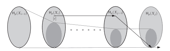
Definition 3.4. (Persistent Betti number) The $p$-th persistent homology groups are the images of the homomorphisms: $\mathrm{H}_p^{i, j}=\operatorname{im} h_p^{i, j}$, for $0 \leq i \leq$ $j \leq n$. The $p$-th persistent Betti numbers are the dimensions $\beta_p^{i, j}=\operatorname{dim} \mathrm{H}_p^{i, j}$ of the vector spaces $\mathrm{H}_p^{i, j}$.
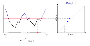
The $p$-th persistent homology groups contain the important information of when a homology class is born or when it dies. The issue of birth and death of a class becomes more subtle because when a new class is born, many other classes that are the sum of this new class and any other existing class are also born. Similarly, when a class ceases to exist, many other classes may cease to exist along with it. Therefore, we need a mechanism to pair births and deaths canonically. Figure $3.7$ illustrates the birth and death of a class, though the pairing of birth and death events is more complicated as stated in Fact 3.3.
Observe that the nontrivial elements of $p$-th persistent homology groups $\mathrm{H}_p^{i, j}$ consist of classes that survive from $X_i$ to $X_j$, that is, the classes which do not get “quotiented out” by the boundaries in $X_j$. So, one can observe the following.
数学代写|表示论代写Representation theory代考|Persistence Diagram
Fact $3.3$ provides a qualitative characterization of the pairing of births and deaths of classes. Now we give a quantitative characterization which helps to draw a visual representation of this pairing called a persistence diagram; see Figure 3.8(a). Consider the extended plane $\overline{\mathbb{R}}^2:=(\mathbb{R} \cup{\pm \infty})^2$ on which we represent the birth at $a_i$ paired with the death at $a_j$ as a point $\left(a_i, a_j\right)$. This pairing uses a persistence pairing function $\mu_p^{i, j}$ defined below. Strictly positive values of this function correspond to multiplicities of points in the persistence diagram (Definition 3.8). In what follows, to account for classes that never die, we extend the induced module in Eq. (3.3) on the right end by assuming that $\mathrm{H}p\left(X{n+1}\right)=0$.
Definition 3.6. For $0<i<j \leq n+1$, define
$$
\mu_p^{i, j}=\left(\beta_p^{i, j-1}-\beta_p^{i, j}\right)-\left(\beta_p^{i-1, j-1}-\beta_p^{i-1, j}\right) .
$$
The first difference on the right-hand side counts the number of independent classes that are born at or before $X_i$ and die entering $X_j$. The second difference counts the number of independent classes that are born at or before $X_{i-1}$ and die entering $X_j$. The difference between the two differences thus counts the number of independent classes that are born at $X_i$ and die entering $X_j$. When $j-n+1, \mu_p^{i, n+1}$ counts the number of independent classes that are born at $X_i$ and die entering $X_{n+1}$. They remain alive till the end in the original filtration without extension, or we say that they never die. To emphasize that classes which exist in $X_n$ actually never die, we equate $n+1$ with $\infty$ and take $a_{n+1}=$ $a_{\infty}=\infty$. Observe that, with this assumption, we have $\beta^{i, n+1}=\beta^{i, \infty}=0$ for every $i \leq n$.
表示论代考
数学代写|表示论代写Representation theory代考|Persistence
在空间和简单过滤的两种情况下 $\mathcal{F}$ ,我们得到一个同源模块:
$$
\mathrm{H} p \mathcal{F}: 0=\mathrm{H}_p\left(X_0\right) \rightarrow \mathrm{H}_p\left(X_1\right) \rightarrow \cdots \rightarrow \mathrm{H}_p\left(X_i\right) \rightarrow h_p^{h_j} \rightarrow \mathrm{H}_p\left(X_j\right) \rightarrow \cdots \rightarrow \mathrm{H}_p\left(X_n\right)=\mathrm{H}_p
$$
在哪里 $X_i=\mathbb{T} a_i$ 如果 $\mathcal{F}$ 是拓扑空间的空间过滤 $X=\mathbb{T}$ 要么 $X_i=K_i$ 如果 $\mathcal{F}$ 是单纯复形的单纯过滤 $X=K$. 同源模块的持久同源群是通过该序列捕获同源类生存的代数结构。一般来说,我们会在Section 中调用同源模块persistence modules3.4认识到我们可以用向量空间代替同调群。
定义 3.4。 (持久的 Betti 号码) $p$-th 持久同源群是同态的图像: $\mathrm{H}_p^{i, j}=\operatorname{im} h_p^{i, j}$ ,为了 $0 \leq i \leq j \leq n$ . 这 $p$-th 持久的 Betti 数字是维度 $\beta_p^{i, j}=\operatorname{dim} \mathrm{H}_p^{i, j}$ 向量空间 $\mathrm{H}_p^{i, j}$.
这 $p$-th 持久同源群包含同源类何时诞生或何时消亡的重要信息。一个类的生雨问题变得更加微妙,因为 当一个新类诞生时,许多其他类也诞生了,这些类是这个新类和任何其他现有类的总和。同样,当一个 类不复存在时,许多其他类也可能随之不复存在。因此,我们需要一种机制来规范地配对出生和死亡。 数字3.7说明了一个类的出生和死亡,尽管如事实 $3.3$ 所述,出生和死亡事件的配对更为复杂。
观察到的非平凡元素 $p$-th 持久同源群 $\mathrm{H}_p^{i, j}$ 由从中幸存下来的类组成 $X_i$ 到 $X_j$ ,也就是说,没有被边界“商 出”的类 $X_j$. 因此,可以观察以下内容。
数学代写|表示论代写Representation theory代考|Persistence Diagram
事实3.3提供了阶级出生和死亡配对的定性特征。现在我们给出一个定量特征,这有助于绘制这种配对的 可视化表示,称为持久性图;见图 3.8(a)。考虑扩展平面 $\bar{R}^2:=(\mathbb{R} \cup \pm \infty)^2$ 我们代表出生于 $a_i$ 与死亡 配对 $a_j$ 作为一个点 $\left(a_i, a_j\right)$. 本次配对使用持久配对功能 $\mu_p^{i, j}$ 定义如下。此函数的严格正值对应于持久性 图中的多个点(定义 3.8) 。接下来,为了解释永不消亡的类,我们扩展了方程式中的诱导模块。(3.3) 在 右端假设 $\mathrm{H} p(X n+1)=0$.
定义 3.6。为了 $0<i<j \leq n+1$ ,定义
$$
\mu_p^{i, j}=\left(\beta_p^{i, j-1}-\beta_p^{i, j}\right)-\left(\beta_p^{i-1, j-1}-\beta_p^{i-1, j}\right) .
$$
右侧的第一个差值计算出生时或之前出生的独立班级的数量 $X_i$ 并死于进入 $X_j$. 第二个差异计算出生在或 之前的独立班级的数量 $X_{i-1}$ 并死于进入 $X_j$. 因此,这两个差异之间的差异计算了出生时独立阶级的数量 $X_i$ 并死于进入 $X_j$. 什么时候 $j-n+1, \mu_p^{i, n+1}$ 计算出生于的独立班级的数量 $X_i$ 并死于进入 $X_{n+1}$. 它们 在原始过滤中一直存活到最后,没有延伸,或者我们说它们永远不会死。强调存在于 $X_n$ 实际上永远不会 死,我们等同于 $n+1$ 和 $\infty$ 并釆取 $a_{n+1}=a_{\infty}=\infty$. 观察到,根据这个假设,我们有 $\beta^{i, n+1}=\beta^{i, \infty}=0$ 每一个 $i \leq n$.

统计代写请认准statistics-lab™. statistics-lab™为您的留学生涯保驾护航。
金融工程代写
金融工程是使用数学技术来解决金融问题。金融工程使用计算机科学、统计学、经济学和应用数学领域的工具和知识来解决当前的金融问题,以及设计新的和创新的金融产品。
非参数统计代写
非参数统计指的是一种统计方法,其中不假设数据来自于由少数参数决定的规定模型;这种模型的例子包括正态分布模型和线性回归模型。
广义线性模型代考
广义线性模型(GLM)归属统计学领域,是一种应用灵活的线性回归模型。该模型允许因变量的偏差分布有除了正态分布之外的其它分布。
术语 广义线性模型(GLM)通常是指给定连续和/或分类预测因素的连续响应变量的常规线性回归模型。它包括多元线性回归,以及方差分析和方差分析(仅含固定效应)。
有限元方法代写
有限元方法(FEM)是一种流行的方法,用于数值解决工程和数学建模中出现的微分方程。典型的问题领域包括结构分析、传热、流体流动、质量运输和电磁势等传统领域。
有限元是一种通用的数值方法,用于解决两个或三个空间变量的偏微分方程(即一些边界值问题)。为了解决一个问题,有限元将一个大系统细分为更小、更简单的部分,称为有限元。这是通过在空间维度上的特定空间离散化来实现的,它是通过构建对象的网格来实现的:用于求解的数值域,它有有限数量的点。边界值问题的有限元方法表述最终导致一个代数方程组。该方法在域上对未知函数进行逼近。[1] 然后将模拟这些有限元的简单方程组合成一个更大的方程系统,以模拟整个问题。然后,有限元通过变化微积分使相关的误差函数最小化来逼近一个解决方案。
tatistics-lab作为专业的留学生服务机构,多年来已为美国、英国、加拿大、澳洲等留学热门地的学生提供专业的学术服务,包括但不限于Essay代写,Assignment代写,Dissertation代写,Report代写,小组作业代写,Proposal代写,Paper代写,Presentation代写,计算机作业代写,论文修改和润色,网课代做,exam代考等等。写作范围涵盖高中,本科,研究生等海外留学全阶段,辐射金融,经济学,会计学,审计学,管理学等全球99%专业科目。写作团队既有专业英语母语作者,也有海外名校硕博留学生,每位写作老师都拥有过硬的语言能力,专业的学科背景和学术写作经验。我们承诺100%原创,100%专业,100%准时,100%满意。
随机分析代写
随机微积分是数学的一个分支,对随机过程进行操作。它允许为随机过程的积分定义一个关于随机过程的一致的积分理论。这个领域是由日本数学家伊藤清在第二次世界大战期间创建并开始的。
时间序列分析代写
随机过程,是依赖于参数的一组随机变量的全体,参数通常是时间。 随机变量是随机现象的数量表现,其时间序列是一组按照时间发生先后顺序进行排列的数据点序列。通常一组时间序列的时间间隔为一恒定值(如1秒,5分钟,12小时,7天,1年),因此时间序列可以作为离散时间数据进行分析处理。研究时间序列数据的意义在于现实中,往往需要研究某个事物其随时间发展变化的规律。这就需要通过研究该事物过去发展的历史记录,以得到其自身发展的规律。
回归分析代写
多元回归分析渐进(Multiple Regression Analysis Asymptotics)属于计量经济学领域,主要是一种数学上的统计分析方法,可以分析复杂情况下各影响因素的数学关系,在自然科学、社会和经济学等多个领域内应用广泛。
MATLAB代写
MATLAB 是一种用于技术计算的高性能语言。它将计算、可视化和编程集成在一个易于使用的环境中,其中问题和解决方案以熟悉的数学符号表示。典型用途包括:数学和计算算法开发建模、仿真和原型制作数据分析、探索和可视化科学和工程图形应用程序开发,包括图形用户界面构建MATLAB 是一个交互式系统,其基本数据元素是一个不需要维度的数组。这使您可以解决许多技术计算问题,尤其是那些具有矩阵和向量公式的问题,而只需用 C 或 Fortran 等标量非交互式语言编写程序所需的时间的一小部分。MATLAB 名称代表矩阵实验室。MATLAB 最初的编写目的是提供对由 LINPACK 和 EISPACK 项目开发的矩阵软件的轻松访问,这两个项目共同代表了矩阵计算软件的最新技术。MATLAB 经过多年的发展,得到了许多用户的投入。在大学环境中,它是数学、工程和科学入门和高级课程的标准教学工具。在工业领域,MATLAB 是高效研究、开发和分析的首选工具。MATLAB 具有一系列称为工具箱的特定于应用程序的解决方案。对于大多数 MATLAB 用户来说非常重要,工具箱允许您学习和应用专业技术。工具箱是 MATLAB 函数(M 文件)的综合集合,可扩展 MATLAB 环境以解决特定类别的问题。可用工具箱的领域包括信号处理、控制系统、神经网络、模糊逻辑、小波、仿真等。