Classical mechanics studies the motion of material bodies. It is among the fundamental branches of modern physics and is therefore an essential component of all graduate programs in Physics. This course introduces the structure of classical mechanics and discusses some of its most important applications in modern physics. In the first part of this course, we will start from the Lagrangian formulation of classical mechanics and study the solution of the equations of motion of several systems, from simple one-body systems, to more complex systems acted upon by central forces and rigid bodies, up to scattering problems and oscillations. We will also extend our discussion to include the theory of special relativity. The second part of this course will introduce the hamiltonian formulation of classical mechanics and study its formal and physical consequences. More advanced topics, such as non-linear dynamics and continuous systems, will be discussed in the third part of this course, depending on time availability.
PREREQUISITES
Classical mechanics studies the motion of material bodies. It is among the fundamental branches of modern physics and is therefore an essential component of all graduate programs in Physics. This course introduces the structure of classical mechanics and discusses some of its most important applications in modern physics. In the first part of this course, we will start from the Lagrangian formulation of classical mechanics and study the solution of the equations of motion of several systems, from simple one-body systems, to more complex systems acted upon by central forces and rigid bodies, up to scattering problems and oscillations. We will also extend our discussion to include the theory of special relativity. The second part of this course will introduce the hamiltonian formulation of classical mechanics and study its formal and physical consequences. More advanced topics, such as non-linear dynamics and continuous systems, will be discussed in the third part of this course, depending on time availability.
Theorem 1.6.2 $A^{-1}$ exists only when $\operatorname{det} A \neq 0$. The elements are then found by: $$ \left(a^{-1}\right){i j}=\frac{U{j i}}{\operatorname{det} A} . $$ (Note the order of the indexes!)
Proof Let $\widehat{A}=\left(\alpha_{i j}=U_{j i}\right)$ be an $(n \times n)$-matrix. With the expansion theorems (1.327) and (1.332) we find: $$ \begin{aligned} & \operatorname{det} A=\sum_j a_{i j} U_{i j}=\sum_j a_{i j} \alpha_{j i}=(A \cdot \widehat{A}){i i}, \ & \operatorname{det} A=\sum_i a{i j} U_{i j}=\sum_i \alpha_{j i} a_{i j}=(\widehat{A} \cdot A){j j} . \ & \end{aligned} $$ The diagonal elements of the product matrices $A \cdot \widehat{A}$ and $\widehat{A} \cdot A$ are thus all identical to $\operatorname{det} A$. What about the non-diagonal elements? With (1.336) one finds: $$ (A \cdot \widehat{A}){i j}=\sum_k a_{i k} \alpha_{k j}=\sum_k a_{i k} U_{j k}=0 \quad \text { for } i \neq j . $$ It follows that $A \cdot \widehat{A}$ and $\widehat{A} \cdot A$ are diagonal matrices with $$ A \cdot \widehat{A}=\widehat{A} \cdot A=\operatorname{det} A \cdot \mathbb{1} $$ With $\operatorname{det} A \neq 0$ and by comparison with (1.337) the theorem is proved: $$ \frac{\widehat{A}}{\operatorname{det} A}=A^{-1} \Longleftrightarrow \frac{U_{j i}}{\operatorname{det} A}=\left(a^{-1}\right)_{i j} . $$
问题 2.
By the term function $f(x)$ one understands the unique attribution of a dependent variable $y$ from the co-domain $W$ to an independent variable $x$ from the domain of definition $D$ of the function $f(x)$ : $$ y=f(x) \quad ; \quad D \subset \mathbb{R} \stackrel{f}{\longrightarrow} W \subset \mathbb{R} . $$ We ask ourselves how $f(x)$ changes with $x$. All elements of the sequence $$ \left{x_n\right}=x_1, x_2, x_3, \cdots, x_n, \cdots $$ shall be from the domain of definition of the function $f$. Then for each $x_n$ there exists a $$ y_n=f\left(x_n\right) $$ and therewith a ‘new’ sequence $\left{f\left(x_n\right)\right}$.
Definition $f(x)$ possesses at $x_0$ a limiting value $f_0$, if for each sequence $\left{x_n\right} \rightarrow x_0$ holds: $$ \lim {n \rightarrow \infty} f\left(x_n\right)=f_0 $$ That is written as: $$ \lim {x \rightarrow x_0} f(x)=f_0 $$ Examples 1. $$ f(x)=\frac{x^3}{x^3+x-1} \quad ; \quad \lim {x \rightarrow \infty} f(x)=? $$ This expression can be reformulated for all $x \neq 0$ : $$ f(x)=\frac{1}{1+\frac{1}{x^2}-\frac{1}{x^3}} . $$ For all sequences $\left{x_n\right}$, which tend to $\infty, \frac{1}{x^2}$ and $\frac{1}{x^3}$ become null sequences. That means: $$ \lim {x \rightarrow \infty} \frac{x^3}{x^3+x-1}=1 $$
Textbooks
• An Introduction to Stochastic Modeling, Fourth Edition by Pinsky and Karlin (freely available through the university library here) • Essentials of Stochastic Processes, Third Edition by Durrett (freely available through the university library here) To reiterate, the textbooks are freely available through the university library. Note that you must be connected to the university Wi-Fi or VPN to access the ebooks from the library links. Furthermore, the library links take some time to populate, so do not be alarmed if the webpage looks bare for a few seconds.
The curl (rotation) of the vector field $\mathbf{a}(\mathbf{r})$ is the vector field $$ \operatorname{rot} \mathbf{a} \equiv \nabla \times \mathbf{a} \equiv \lim {V \rightarrow 0} \frac{1}{V} \int{(V)} \mathbf{d} \mathbf{f} \times \mathbf{a} $$ For the above-mentioned cube with the edges $\mathrm{d} x, \mathrm{~d} y, \mathrm{~d} z$, the $x$-component of the right-hand expression is equal to $$ \frac{1}{\mathrm{~d} x \mathrm{~d} y \mathrm{~d} z}\left[+\mathrm{d} z \mathrm{~d} x\left{a_{z}(x, y+\mathrm{d} y, z)-a_{z}(x, y, z)\right}\right. $$ $$ \left.-\mathrm{d} x \mathrm{~d} y\left{a_{y}(x, y, z+\mathrm{d} z)-a_{y}(x, y, z)\right}\right]=\frac{\partial a_{z}}{\partial y}-\frac{\partial a_{y}}{\partial z} . $$ With $\partial_{i} \equiv 1 / \partial x_{i}$, we thus have which is the vector product of the operators $\nabla$ and a. This explains the notation $\boldsymbol{\nabla} \times \mathbf{a}$. Moreover, we have $$ \int_{V} \mathrm{~d} V \nabla \times \mathbf{a}=\int_{(V)} \mathrm{d} \mathbf{f} \times \mathbf{a} $$ for all continuous vector fields, although they may become singular point-wise, and even along lines, as will become apparent shortly. An important result is Stokes’s theorem $$ \int_{A} \mathrm{df} \cdot(\nabla \times \mathbf{a})=\int_{(A)} \mathrm{d} \mathbf{r} \cdot \mathbf{a} $$ where $\mathrm{df}$ is taken in the rotational sense on the edge $(A)$ and forms a right=hand screw.
物理代写|理论力学代写theoretical mechanics代考|Delta Function
In the following, we shall often use the Dirac delta function. Therefore, its properties are compiled here, even though it does not actually belong to vector analysis, but to general analysis (and in particular to integral calculus). We start with the Kronecker symbol $$ \delta_{i k}= \begin{cases}0 & \text { for } i \neq k \ 1 & \text { for } i=k\end{cases} $$ It is useful for many purposes. In particular we may use it to filter out the $k$ th element of a sequence $\left{f_{i}\right}$ : $$ f_{k}=\sum_{i} f_{i} \delta_{i k} . $$ Here, of course, within the sum, one of the $i$ has to take the value $k$. Now, if we make the transition from the countable (discrete) variables $i$ to a continuous quantity $x$, then we must also generalize the Kronecker symbol. This yields Dirac’s delta function $\delta\left(x-x^{\prime}\right)$. It is defined by the equation $$ f\left(x^{\prime}\right)=\int_{a}^{b} f(x) \delta\left(x-x^{\prime}\right) \mathrm{d} x \quad \text { for } a<x^{\prime}<b, \text { zero otherwise }, $$ where $f(x)$ is an arbitrary continuous test function. If the variable $x$ (and hence also $\mathrm{d} x)$ is a physical quantity with unit $[x]$, the delta function has the unit $[x]^{-1}$.
Obviously, the delta function $\delta\left(x-x^{\prime}\right)$ is not an ordinary function, because it has to vanish for $x \neq x^{\prime}$ and it has to be singular for $x=x^{\prime}$, so that the integral becomes $\int \delta\left(x-x^{\prime}\right) \mathrm{d} x=1$. Consequently, we have to extend the concept of a function: $\delta\left(x-x^{\prime}\right)$ is a distribution, or generalized function, which makes sense only as a weight factor in an integrand, while an ordinary function $y=f(x)$ is a map $x \rightarrow y$. Every equation in which the delta function appears without an integral symbol is an equation between integrands: on both sides of the equation, the integral symbol and the test function have been left out. The delta function is the derivative of the Heaviside step function: $$ \varepsilon\left(x-x^{\prime}\right)=\left{\begin{array}{ll} 0 & \text { for } xx^{\prime} \end{array} \quad \Longrightarrow \quad \delta(x)=\varepsilon^{\prime}(x)\right. $$
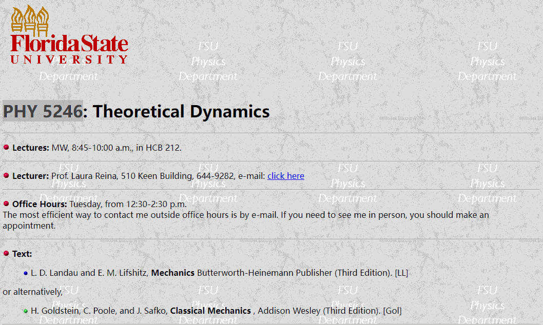
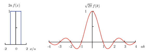
If the region of definition is infinite on both sides, we use $$ f(x)=\int_{-\infty}^{\infty} g(k, x) f(k) \mathrm{d} k, \quad f(k)=\int_{-\infty}^{\infty} g^{}(k, x) f(x) \mathrm{d} x $$ with $g(k, x)=1 / \sqrt{2 \pi} \exp (\mathrm{i} k x)$ : $$ \begin{aligned} &f(x)=\frac{1}{\sqrt{2 \pi}} \int_{-\infty}^{\infty} \exp (+\mathrm{i} k x) f(k) \mathrm{d} k \ &f(k)=\frac{1}{\sqrt{2 \pi}} \int_{-\infty}^{\infty} \exp (-\mathrm{i} k x) f(x) \mathrm{d} x \end{aligned} $$ Generally, $f(x)$ and $f(k)$ are different functions of their arguments, but we would like to distinguish them only through their argument. [The less symmetric notation $f(x)=\int \exp (\mathrm{i} k x) F(k) \mathrm{d} k$ with $F(k)=f(k) / \sqrt{2 \pi}$ is often used. This avoids the square root factor with the agreement that $(2 \pi)^{-1}$ always appears with $\mathrm{d} x$.] Instead of the pair of variables $x \leftrightarrow k$, the pair $t \leftrightarrow \omega$ is also often used. Important properties of the Fourier transform are $f(x)=f^{}(x) \quad \Longleftrightarrow \quad f(k)=f^{*}(-k)$, $f(x)=g(x) h(x) \Longleftrightarrow f(k)=\frac{1}{\sqrt{2 \pi}} \int_{-\infty}^{\infty} g\left(k-k^{\prime}\right) h\left(k^{\prime}\right) \mathrm{d} k^{\prime}$, $f(x)=g\left(x-x^{\prime}\right) \quad \Longleftrightarrow \quad f(k)=\exp \left(-\mathrm{i} k x^{\prime}\right) g(k) .$ For a periodic function $f(x)=f(x-l)$ the last relation leads to the condition $k_{n}=$ $2 \pi n / l$ with $n \in{0, \pm 1, \pm 2, \ldots}$, thus to a Fourier series instead of the integral. In addition, by Fourier transform, all convolution integrals $\int g\left(x-x^{\prime}\right) h\left(x^{\prime}\right) \mathrm{d} x^{\prime}$ can clearly be turned into products $\sqrt{2 \pi} g(k) h(k)$ (Problem 3.9), which are much easier to handle.
If a vector is associated with each position, we speak of a vector field. With scalar fields, a scalar is associated with each position. The vector field $\mathbf{a}(\mathbf{r})$ is only continuous at $\mathbf{r}{0}$ if all paths approaching $\mathbf{r}{0}$ have the same limit. For scalar fields, this is already an essentially stronger requirement than in one dimension.
Instead of drawing a vector field with arrows at many positions, it is often visualized by a set of field lines: at every point of a field line the tangent points in the direction of the vector field. Thus $\mathbf{a} | \mathrm{d} \mathbf{r}$ and $\mathbf{a} \times \mathrm{d} \mathbf{r}=\mathbf{0}$.
For a given vector field many integrals can be formed. In particular, we often have to evaluate integrals over surfaces or volumes. In order to avoid double or triple integral symbols, the corresponding differential is often written immediately after the integral symbol: $\mathrm{d} V$ for the volume, df for the surface integral, e.g., $\int \mathrm{d} \mathbf{f} \times \mathbf{a}$ instead of $-\int \mathbf{a} \times$ df (in this way the unnecessary minus sign is avoided for the introduction of the curl density or rotation on p. 13). Here df is perpendicular to the related surface element. However, the sign of df still has to be fixed. In general, we consider the surface of a volume $V$, which will be denoted here by $(V)$. Then df points outwards. Corresponding to $(V)$, the edge of an area $A$ is denoted by $(A)$. An important example of a scalar integral is the line integral $\int \mathrm{d} \mathbf{r} \cdot \mathbf{a}(\mathbf{r})$ along a given curve $\mathbf{r}(t)$. If the parameter $t$ determines the points on the curve uniquely, then the line integral $$ \int \mathrm{d} \mathbf{r} \cdot \mathbf{a}(\mathbf{r})=\int \mathrm{d} t \frac{\mathrm{d} \mathbf{r}}{\mathrm{d} t} \cdot \mathbf{a}(\mathbf{r}(t)) $$ is an ordinary integral over the scalar product $\mathbf{a} \cdot \mathrm{d} \mathbf{r} / \mathrm{d} t$. Another example of a scalar integral is the surface integral $\int \mathrm{df} \cdot \mathbf{a}(\mathbf{r})$ taken over a given area $A$ or over the surface $(V)$ of the volume $V$.
Besides the scalar integrals, vectorial integrals like $\int \mathrm{d} V \mathbf{a}, \int \mathrm{d} \mathbf{f} \times \mathbf{a}$, and $\int \mathrm{d} \mathbf{r} \times \mathbf{a}$ can arise, e.g., the $x$-component of $\int \mathrm{d} V$ a is the simple integral $\int \mathrm{d} V a_{x}$.
Different forms are also reasonable through differentiation: vector fields can be deduced from scalar fields, and scalar fields (but also vector fields and tensor fields) from vector fields. These will now be considered one by one. Then the operator $\nabla$ will always turn up. The symbol $\nabla$, an upside-down $\Delta$, resembles an Ancient Greek harp and hence is called nabla, after W. R. Hamilton (see 122).
物理代写|理论力学代写theoretical mechanics代考|Gradient
The gradient of a scalar function $\psi(\mathbf{r})$ is the vector field $$ \operatorname{grad} \psi \equiv \nabla \psi, \quad \text { with } \nabla \psi \cdot \mathrm{d} \mathbf{r} \equiv \mathrm{d} \psi \equiv \psi(\mathbf{r}+\mathrm{d} \mathbf{r})-\psi(\mathbf{r}) $$ This is clearly perpendicular to the area $\psi=$ const. at every point and points in the direction of $\mathrm{d} \psi>0$ (see Fig. 1.4). The value of the vector $\nabla \psi$ is equal to the derivative of the scalar function $\psi(\mathbf{r})$ with respect to the line element in this direction. In Cartesian coordinates, we thus have $$ \nabla \psi=\mathbf{e}{x} \frac{\partial \psi}{\partial x}+\mathbf{e}{y} \frac{\partial \psi}{\partial y}+\mathbf{e}{z} \frac{\partial \psi}{\partial z}=\left(\mathbf{e}{x} \frac{\partial}{\partial x}+\mathbf{e}{y} \frac{\partial}{\partial y}+\mathbf{e}{z} \frac{\partial}{\partial z}\right) \psi $$
Here $\partial \psi / \partial x$ is the partial derivative of $\psi(x, y, z)$ with respect to $x$ for constant $y$ and $z$. (If other quantities are kept fixed instead, then special rules have to be considered, something we shall deal with in Sect. 1.2.7.) The gradient is also obtained as a limit of a vectorial integral: $$ \nabla \psi=\lim {V \rightarrow 0} \frac{1}{V} \int{(V)} \text { df } \psi(\mathbf{r}) $$ If we take a cube with infinitesimal edges $\mathrm{d} x, \mathrm{~d} y$, and $\mathrm{d} z$, we have on the right-hand side as $x$-component $(\mathrm{d} x \mathrm{~d} y \mathrm{~d} z)^{-1}{\mathrm{~d} y \mathrm{~d} z \psi(x+\mathrm{d} x, y, z)-\mathrm{d} y \mathrm{~d} z \psi(x, y, z)}=$ $\partial \psi / \partial x$, and similarly for the remaining components. Hence, also $$ \int_{V} \mathrm{~d} V \nabla \psi-\int_{(V)} \mathrm{d} \mathbf{f} \psi $$ because a finite volume can be divided into infinitesimal volume elements, and for continuous $\psi$, contributions from adjacent planes cancel in pairs. With this surface integral the gradient can be determined even if $\psi$ is not differentiable (singular) at individual points-the surface integral depends only upon points in the neighbourhood of the singular point, where everything is continuous. (In Sect. 1.1.12, we shall consider the example $\psi=1 / r$.)
物理代写|理论力学代写theoretical mechanics代考|Divergence
While a vector field has been derived from a scalar field with the help of the gradient, the divergence associates a scalar field with a vector field: $$ \operatorname{div} \mathbf{a} \equiv \nabla \cdot \mathbf{a} \equiv \lim {V \rightarrow 0} \frac{1}{V} \int{(V)} \mathbf{d f} \cdot \mathbf{a} $$
For the same cube as in the last section, the right-hand expression yields $$ \begin{aligned} \frac{1}{\mathrm{~d} x \mathrm{~d} y \mathrm{~d} z} & {\left[\mathrm{~d} y \mathrm{~d} z\left{a_{x}(x+\mathrm{d} x, y, z)-a_{x}(x, y, z)\right}\right.} \ &+\mathrm{d} z \mathrm{~d} x\left{a_{y}(x, y+\mathrm{d} y, z)-a_{y}(x, y, z)\right} \ &\left.+\mathrm{d} x \mathrm{~d} y\left{a_{z}(x, y, z+\mathrm{d} z)-a_{z}(x, y, z)\right}\right]=\frac{\partial a_{x}}{\partial x}+\frac{\partial a_{y}}{\partial y}+\frac{\partial a_{z}}{\partial z} \end{aligned} $$ as suggested by the notation $\nabla$. a, i.e., a scalar product between the vector operator $\nabla$ and the vector $\mathbf{a}$. With this we have also proven Gauss’s theorem $$ \int_{V} \mathrm{~d} V \nabla \cdot \mathbf{a}=\int_{(V)} \mathrm{d} \mathbf{f} \cdot \mathbf{a} $$ since for any partition of the finite volume $V$ into infinitesimal ones and for a continuous vector field $\mathbf{a}$, the contributions of adjacent planes cancel in pairs. The integrals here may even enclose points at which a (r) is singular (see Fig. 1.5 left). We shall discuss this in more detail in Sect. 1.1.12.
The integral $\int$ df $\cdot \mathbf{a}$ over an area is called the $\int u x$ of the vector field $\mathbf{a}(\mathbf{r})$ through this area (even if $\mathbf{a}$ is not a current density). In this picture, the integral over the closed area $(V)$ describes the source strength of the vector field, i.e., how much more flows into $V$ than out. The divergence is therefore to be understood as a source density. A vector field is said to be source-free if its divergence vanishes everywhere. (If the source density is negative, then “drains” predominate.)
The concept of a field-line tube is also useful (we discussed field lines in Sect. 1.1.4). Its walls are everywhere parallel to a (r). Therefore, there is no flux through the walls, and the flux through the end faces is equal to the volume integral of $\nabla \cdot \mathbf{a}$. For a source-free vector field $(\nabla \cdot \mathbf{a}=0)$, the flux flowing into the field-line tube through one end face emerges again from the other.
标量函数的梯度 $\psi(\mathbf{r})$ 是向量场 $$ \operatorname{grad} \psi \equiv \nabla \psi, \quad \text { with } \nabla \psi \cdot \mathrm{d} \mathbf{r} \equiv \mathrm{d} \psi \equiv \psi(\mathbf{r}+\mathrm{d} \mathbf{r})-\psi(\mathbf{r}) $$ 这显然垂直于该区域 $\psi=$ 常量。在每个点和指向的方向 $\mathrm{d} \psi>0$ (见图 1.4) 。向量的值 $\nabla \psi$ 等于标量函数的导数 $\psi(\mathbf{r})$ 相对于这个方向的线元素。在笛卡尔坐标中,我们因此有 $$ \nabla \psi=\mathbf{e} x \frac{\partial \psi}{\partial x}+\mathbf{e} y \frac{\partial \psi}{\partial y}+\mathbf{e} z \frac{\partial \psi}{\partial z}=\left(\mathbf{e} x \frac{\partial}{\partial x}+\mathbf{e} y \frac{\partial}{\partial y}+\mathbf{e} z \frac{\partial}{\partial z}\right) \psi $$ 这里 $\partial \psi / \partial x$ 是的偏导数 $\psi(x, y, z)$ 关于 $x$ 为常数 $y$ 和 $z$. (如果其他量保持不变,则必须考虑特殊规则,我们将在第 $1.2 .7$ 节中讨论。) 梯度也作为矢量积分的极限获得: $$ \nabla \psi=\lim V \rightarrow 0 \frac{1}{V} \int(V) \mathrm{df} \psi(\mathbf{r}) $$ 如果我们取一个具有无穷小边的立方体 $\mathrm{d} x, \mathrm{~d} y$ ,和 $\mathrm{d} z$ ,我们在右边有 $x$-零件 $(\mathrm{d} x \mathrm{~d} y \mathrm{~d} z)^{-1} \mathrm{~d} y \mathrm{~d} z \psi(x+\mathrm{d} x, y, z)-\mathrm{d} y \mathrm{~d} z \psi(x, y, z)=\partial \psi / \partial x$ ,对于其余的组件也是如此。因此,也 $$ \int_{V} \mathrm{~d} V \nabla \psi-\int_{(V)} \mathrm{d} \mathbf{f} \psi $$ 因为一个有限的体积可以分成无穷小的体积元素,而对于连续的 $\psi$ ,来自相邻平面的贡献成对抵消。使用这个表面 积分,即使在以下情况下也可以确定梯度 $\psi$ 在单个点上是不可微的(奇异的) – 曲面积分仅取决于奇异点附近的 点,其中一切都是连续的。(在第 $1.1 .12$ 节中,我们将考虑这个例子 $\psi=1 / r$.)
物理代写|理论力学代写theoretical mechanics代考|Divergence
虽然向量场是在梯度的帮助下从标量场导出的,但散度将标量场与向量场相关联: $\$ \$$ loperatorname{div} \mathbf{a} \equiv $\backslash$ nabla $\backslash$ cdot $\backslash$ mathbf ${$ a $}$ lequiv $\backslash \lim {V \backslash$ Irightarrow 0$} \backslash$ frac ${1} V} \backslash$ Iint ${(\mathrm{V})} \mathrm{~ I m a t h b f { d f } ~ \ c d o t ~ \ m a t h b f { a }}$ $\$ \$$ 对于与上一节中相同的立方体,右侧表达式产生 Ibegin ${a l i g n} \backslash$ frac ${1} \backslash \backslash m a t h r m{\sim d} x \backslash m a t h r m{\sim d}$ 和 $\backslash$ mathrm ${\sim d}$ Z \& ${\backslash \backslash$ eft $\backslash \backslash m a t h r m{\sim d}$ 和 $\backslash$ mathrm ${\sim d}}$ Z $\backslash$ eft ${a$ 正如符号所建议的那样 $\nabla$. a,即向量算子之间的标量积 $\nabla$ 和向量 $\mathbf{a}$. 这样我们也证明了高斯定理 $$ \int_{V} \mathrm{~d} V \nabla \cdot \mathbf{a}=\int_{(V)} \mathrm{d} \mathbf{f} \cdot \mathbf{a} $$ 因为对于有限体积的任何分区 $V$ 成无穷小和连续向量场 $\mathbf{a}$ ,相邻平面的贡献成对抵消。这里的积分甚至可以包含 $a$ (r) 为奇异的点 (见图 $1.5$ 左) 。我们将在第 3 节中更详细地讨论这个问题。1.1.12。 积分 $\int \mathrm{df} \cdot \mathbf{a}$ 在一个区域上称为 $\int u x$ 向量场的 $\mathbf{a}(\mathbf{r})$ 通过这个区域(即使 $\mathbf{a}$ 不是电流密度)。在这张图中,封闭区域上 的积分 $(V)$ 描述矢量场的源强度,即有多少流入 $V$ 比出来。因此,该分歧应被理解为源密度。如果矢量场的散度处 处消失,则称矢量场是无源的。(如果源密度为负,则漏极”占主导地位。) 场线管的概念也很有用(我们在第 $1.1 .4$ 节中讨论了场线)。它的墙壁处处平行于 $a(r)$ 。因此,没有通过壁的通 量,通过端面的通量等于体积积分 $\nabla \cdot \mathbf{a}$. 对于无源矢量场 $(\nabla \cdot \mathbf{a}=0)$ ,通过一个端面流入场线管的通量从另一个 端面再次出现。
Space and time are two basic concepts which, according to Kant, inherently or innately determine the form of all experience in an a priori manner, thereby making possible experience as such: only in space and time can we arrange our sensations. [According to the doctrines of evolutionary cognition, what is innate to us has developed phylogenetically by adaption to our environment. This is why we only notice the insufficiency of these “self-evident”‘ concepts under extraordinary circumstances, e.g., for velocities close to that of light $\left(c_{0}\right)$ or actions of the order of Planck’s quantum $h$. We shall tackle such “weird” cases later-in electromagnetism and quantum mechanics. For the time being, we want to make sure we can handle our familiar environment.]
To do this, we introduce a continuous parameter $t$. Like every other physical quantity it is composed of number and unit (for example, a second $1 \mathrm{~s}=1 \mathrm{~min} / 60$ $-1 \mathrm{~h} / 3600$ ). The larger the unit, the smaller the number. Physical quantities do not depend on the unit-likewise equations between physical quantities. Nevertheless, the opposite is sometimes seen, as in: “We choose units such that the velocity of light $c$ assumes the value 1”. In fact, the concept of velocity is thereby changed, so that instead of the velocity $v$, the ratio $v / c$ is taken here as the velocity, and $c t$ as time or $x / c$ as length.
The zero time $(t=0)$ can be chosen arbitrarily, since basically only the time difference, i.e., the duration of a process, is important. A differentiation with respect to time $(\mathrm{d} / \mathrm{d} t)$ is often marked by a dot over the differentiated quantity, i.e., $\mathrm{d} x / \mathrm{d} t \equiv \dot{x}$. In empty space every direction is equivalent. Here, too, we may choose the zero point freely and, starting from this point, determine the position of other points in a coordinate-free notation by the position vector $\mathbf{r}$, which fixes the distance and direction of the point under consideration. This coordinate-free type of notation is particularly advantageous when we want to exploit the assumed homogeneity of space. However, conditions often arise (i.e., when there is axial or spherical symmetry) which are best taken care of in special coordinates. We are free to choose a coordinate system. We only require that it determine all positions uniquely. This we shall treat in the next section.
物理代写|理论力学代写theoretical mechanics代考|Vector Algebra
From two vectors $\mathbf{a}$ and $\mathbf{b}$, their sum $\mathbf{a}+\mathbf{b}$ may be formed according to the construction of parallelograms (as the diagonal), as shown in Fig. 1.1. From this follows the commutative and associative law of vector addition: $$ \mathbf{a}+\mathbf{b}=\mathbf{b}+\mathbf{a}, \quad(\mathbf{a}+\mathbf{b})+\mathbf{c}=\mathbf{a}+(\mathbf{b}+\mathbf{c}) $$ The product of the vectors a with a scalar (i.e., directionless) factor $\alpha$ is understood as the vector $\alpha \mathbf{a}=\mathbf{a} \alpha$ with the same (for $\alpha<0$ opposite) direction and with value $|\alpha| a$. In particular, a and $-\mathbf{a}$ have the same value, but opposite directions. For $\alpha=0$ the zero vector 0 results, with length 0 and undetermined direction.
The scalar product (inner product) $\mathbf{a} \cdot \mathbf{b}$ of the two vectors $\mathbf{a}$ and $\mathbf{b}$ is the product of their values times the cosine of the enclosed angle $\phi_{a b}$ (see Fig. 1.2 left): $$ \mathbf{a} \cdot \mathbf{b} \equiv a b \cos \phi_{a b} $$ The dot between the two factors is important for the scalar product-if it is missing, then it is the tensor product of the two vectors, which will be explained in Sect. 1.2.4 with $\mathbf{a} \cdot \mathbf{b} \mathbf{c} \neq \mathbf{a} \mathbf{b} \cdot \mathbf{c}$, if $\mathbf{a}$ and $\mathbf{c}$ have different directions, i.e., if $\mathbf{a}$ is not a multiple of $\mathbf{c}$. Consequently, one has $$ \mathbf{a} \cdot \mathbf{b}=\mathbf{b} \cdot \mathbf{a} $$ and $$ \mathbf{a} \cdot \mathbf{b}=0 \quad \Longleftrightarrow \quad \mathbf{a} \perp \mathbf{b} \text { or } a=0 \text { or } b=0 . $$ If the two vectors are oriented perpendicularly to each other $(\mathbf{a} \perp \mathbf{b})$, then they are also said to be orthogonal. Obviously, $\mathbf{a} \cdot \mathbf{a}=a^{2}$ holds. Vectors with value 1 are called unit vectors. Here they are denoted by e. Given three Cartesian, i.e., pairwise perpendicular unit vectors $\mathbf{e}{x}, \mathbf{e}{y}, \mathbf{e}{z}$, all vectors can be decomposed in terms of these: $$ \mathbf{a}=\mathbf{e}{x} a_{x}+\mathbf{e}{y} a{y}+\mathbf{e}{z} a{z}, $$ with the Cartesian components $$ a_{x} \equiv \mathbf{e}{x} \cdot \mathbf{a}, \quad a{y} \equiv \mathbf{e}{y} \cdot \mathbf{a}, \quad a{z} \equiv \mathbf{e}_{z} \cdot \mathbf{a} . $$
物理代写|理论力学代写theoretical mechanics代考|Trajectories
If a vector depends upon a parameter, then we speak of a vector function. The vector function $\mathbf{a}(t)$ is continuous at $t_{0}$, if it tends to $\mathbf{a}\left(t_{0}\right)$ for $t \rightarrow t_{0}$. With the same limit $t \rightarrow t_{0}$, the vector differential da and the first derivative da/d $t$ is introduced. These quantities may be formed for every Cartesian component, and we have $$ \begin{array}{ll} \mathrm{d}(\mathbf{a}+\mathbf{b})=\mathrm{d} \mathbf{a}+\mathrm{d} \mathbf{b}, & \mathrm{d}(\alpha \mathbf{a})=\alpha \mathrm{d} \mathbf{a}+\mathbf{a} \mathrm{d} \alpha \ \mathrm{d}(\mathbf{a} \cdot \mathbf{b})=\mathbf{a} \cdot \mathrm{d} \mathbf{b}+\mathbf{b} \cdot \mathrm{d} \mathbf{a}, & \mathrm{d}(\mathbf{a} \times \mathbf{b})=\mathbf{a} \times \mathrm{d} \mathbf{b}-\mathbf{b} \times \mathrm{d} \mathbf{a} \end{array} $$ Obviously, $\mathbf{a} \cdot \mathrm{d} \mathbf{a} / \mathrm{d} t=\frac{1}{2} \mathrm{~d}(\mathbf{a} \cdot \mathbf{a}) / \mathrm{d} t=\frac{1}{2} \mathrm{~d} a^{2} / \mathrm{d} t=a \mathrm{~d} a / \mathrm{d} t$ holds. In particular the derivative of a unit vector is always perpendicular to the original vector-if it does nôt vañish.
As an example of a vector function, we investigate $\mathbf{r}(t)$, the path of a point as a function of the time $t$. Thus we want to consider also the velocity $\mathbf{v}=\dot{\mathbf{r}}$ and the acceleration $\mathbf{a}=\ddot{\mathbf{r}}$ rather generally. The time is not important for the trajectories as geometrical lines. Therefore, instead of the time $t$ we introduce the path length $s$ as a parameter and exploit $\mathrm{d} s=|\mathrm{d} \mathbf{r}|=v \mathrm{~d} t$.
We now take three mutually perpendicular unit vectors $\mathbf{e}{\mathrm{T}}, \mathbf{e}{\mathrm{N}}$, and $\mathbf{e}{\mathrm{B}}$, which are attached to every point on the trajectory. Here $\mathbf{e}{\mathrm{T}}$ has the direction of $\mathbf{v}$ : tangent vector $\quad \mathbf{e}{\mathrm{T}} \equiv \frac{\mathrm{d} \mathbf{r}}{\mathrm{d} s}=\frac{\mathbf{v}}{v}$ For a straight path, this vector is already sufficient for the description. But in general the path curvature $\quad \kappa \equiv\left|\frac{\mathrm{d} \mathbf{e}{\mathrm{T}}}{\mathrm{d} s}\right|=\left|\frac{\mathrm{d}^{2} \mathbf{r}}{\mathrm{d} s^{2}}\right|$ is different from zero. In order to get more insight into this parameter we consider a plane curve of constant curvature, namely, the circle with $s=R \varphi$. For $\mathbf{r}(\varphi)=\mathbf{r}{0}+$ $R\left(\cos \varphi \mathbf{e}{x}+\sin \varphi \mathbf{e}{y}\right)$, we have $\kappa=\left|\mathrm{d}^{2} \mathbf{r} / \mathrm{d}(R \varphi)^{2}\right|=R^{-1}$. Instead of the curvature $\kappa$, its reciprocal, the curvature radius $R \equiv \frac{1}{\kappa}$, can also be used to determine the curve. Hence as a further unit vector we have the normal vector $\quad \mathbf{e}{\mathrm{N}} \equiv R \frac{\mathbf{d} \mathbf{e}_{\mathrm{T}}}{\mathrm{d} s}=R \frac{\mathrm{d}^{2} \mathbf{r}}{\mathrm{d} s^{2}}$
物理代写|理论力学代写theoretical mechanics代考|Homogenization of Piezoelectric Composites
To determine the effective properties of piezoelectric composites, in ACELANCOMPOS package we use classical version of the effective moduli method. For piezoelectric composites this method was applied in a large number of papers $[5,9$, $22,24,30]$, with its mathematical basis given in $[22,24]$. In this section, we describe the formulation of the homogenization problem using the Voigt vector-matrix notation, which is generally accepted in the physical and theoretical literature on piezoelectricity.
The input data for the homogenization problem for two-phase piezoelectric (electroelastic) composite material is its representative volume element $\Omega$ together with the parts $\Omega^{(1)}$ and $\Omega^{(2)}$ filled with materials of different phases. In the domains $\Omega^{(j)}, j=1,2$, the following material moduli are known: the elastic stiffnesses $c_{\alpha \beta}^{E}=c_{\alpha \beta}^{E(j)}$, measured at constant electric field; the piezoelectric moduli $e_{k \beta}=e_{k \beta}^{(j)}$; and the dielectric permittivity constants $\varepsilon_{k m}^{S}=\varepsilon_{k m}^{S(j)}$, measured at constant strain; $\alpha, \beta=1,2, \ldots, 6, k, m=1,2,3 ; \mathbf{x} \in \Omega^{(j)} .$
We also introduce the following notation: $\Gamma=\partial \Omega$ is the outer boundary of the volume; $\mathbf{u}=\mathbf{u}(\mathbf{x})$ is the vector function of displacements; $\varphi=\varphi(\mathbf{x})$ is the electric potential function; $\mathbf{T}=\left{\sigma_{11}, \sigma_{22}, \sigma_{33}, \sigma_{23}, \sigma_{13}, \sigma_{12}\right}$ is the array of stress components $\sigma_{k m} ; \mathbf{S}=\left{\varepsilon_{11}, \varepsilon_{22}, \varepsilon_{33}, 2 \varepsilon_{23}, 2 \varepsilon_{13}, 2 \varepsilon_{12}\right}$ is the array of the strain components $\varepsilon_{k m} ; \mathbf{D}$ is the vector of electric induction or electric displacement; $\mathbf{E}$ is the vector of electric field; $\mathbf{c}^{E}$ is the $6 \times 6$ matrix of elastic stiffness moduli $c_{\alpha \beta}^{E}$, e is the $3 \times 6$ matrix of piezoelectric modui $e_{k \beta} ; \varepsilon^{s}$ is the $3 \times 3$ matrix of dielectric permittivity moduli $\varepsilon_{k m m^{}}^{S}$. In the homogenization problem, it is necessary to determine the effective moduli $\bar{c}{\alpha \beta}^{E}, \bar{e}{k \beta}, \bar{\varepsilon}_{k m m}^{S}$. In order to do this, we need to solve a set of static boundary piezoelectric problems $$ \begin{gathered} \mathbf{L}^{}(\nabla) \cdot \mathbf{T}=0, \quad \nabla \cdot \mathbf{D}=0, \quad \mathbf{x} \in \Omega \ \mathbf{T}=\mathbf{c}^{E} \cdot \mathbf{S}-\mathbf{e}^{*} \cdot \mathbf{E}=0, \quad \mathbf{D}=\mathbf{e} \cdot \mathbf{S}+\boldsymbol{\varepsilon}^{S} \cdot \mathbf{E}=0 \end{gathered} $$
$$ \begin{gathered} \mathbf{S}=\mathbf{L}(\nabla) \cdot \mathbf{u}, \quad \mathbf{E}=-\nabla \varphi \ \mathbf{u}=\mathbf{L}^{}(\mathbf{x}) \cdot \mathbf{S}{0}, \quad \varphi=-\mathbf{x} \cdot \mathbf{E}{0}, \quad \mathbf{x} \in \Gamma \end{gathered} $$ where $\mathbf{S}{0}$ is the six-dimensional array of constant values, $\mathbf{E}{0}$ is the constant vector, $(\ldots)^{}$ is the transpose operation, $L(\nabla)$ is the matrix operator of differentiation, which in transposed form is defined as follows $$ \mathbf{L}^{*}(\nabla)=\left[\begin{array}{cccccc} \partial_{1} & 0 & 0 & 0 & \partial_{3} & \partial_{2} \ 0 & \partial_{2} & 0 & \partial_{3} & 0 & \partial_{1} \ 0 & 0 & \partial_{3} & \partial_{2} & \partial_{1} & 0 \end{array}\right] $$
物理代写|理论力学代写theoretical mechanics代考|Some Models of Inhomogeneous Polarization
When analyzing the composites with the skeleton made of elastic piezoceramic material containing inclusions or pores, we can expect high inhomogeneity of the residual polarization vector P of piezoceramics. Indeed, even if the piezoceramics are polarized in one direction, the electric field or electric induction vectors inside the composite will not be parallel to this direction but will go around the inhomogeneities of the composite. Then it is logical to assume that the directions of the vector $\mathbf{P}=\mathbf{P}(\mathbf{x})$ at the first approximation can be obtained from the solution of the model problem of the polarization of composite material in linear setting. We will provide the mathematical setting of this problem in relation to the subsequent finite element homogenization problem.
Let $\Omega$ be a cubic representative volume of the composite of the size $L \times L \times L$ with the mesh consisting of finite elements $\Omega^{e m}, \Omega=\cup_{m} \Omega^{e m}$. It is assumed that each element $\Omega^{e m}$ belongs to the domain of one of the two phases, namely, the unpolarized piezoceramics $\Omega^{(1)}$ or the inclusion $\Omega^{(2)}$. Consequently, each element $\Omega^{e m}$ has dielectric properties of two phases, which we will consider isotropic materials with dielectric permeabilities $\varepsilon_{i}=\varepsilon_{i}^{(j)}, \mathbf{x} \in \Omega^{(j)}, j=1,2$. We assume that the edges $x_{3}=0$ and $x_{3}=L$ of the volume $\Omega$ are electrodized and are subjected to the potential difference $\Delta V=L E_{}$ with the field value $E_{}$, which is enough for the polarization of homogeneous piezoceramic material.
For the representative volume $\Omega$ with the help of FEM we solve the problem of electrostatics $$ \begin{gathered} \nabla \cdot \mathbf{D}=0, \quad \mathbf{D}=\varepsilon_{i} \mathbf{E}, \quad \mathbf{E}=-\nabla \varphi, \quad \mathbf{x} \in \Omega, \ \varphi=L E_{4}, \quad x_{3}=0 ; \quad \varphi=0, \quad x_{3}=L . \end{gathered} $$
ACELAN-COMPOS is a client-server GUI application with a modular structure. The user interface is implemented as an application developed using HTML and JavaScript and runs in a web-browser. The client-side application consists of the following moduli:
Graphic 3D preprocessor – a component for creating and viewing the source geometry. It is developed using the WebGL Framework. Currently, to start solving the problem the user provides parameters for the new model, including preferred connectivity type. Then the preprocessor allows analyzing generated mesh.
Tools for editing physical models – a set of forms for specifying boundary conditions and material properties with the help of the ACELAN command language.
Graphic 3D postprocessor – a module for analyzing the solution obtained, which includes the ability to view the solution both in tabular form and in the form of visualizations over the original geometry. Supported viewing modes include heat maps, vector field visualizations, sections and body viewing capabilities, etc. WebGL Framework is also selected as the implementation tool for the graphic postprocessor.
The server-side part of the package is a cross-platform application, developed using the .Net Core Framework and the $\mathrm{C} #$ programming language. It is responsible for performing calculations and processing the results of solving the problem. It allows performing computations for different users simultaneously. The interaction between the server and the client application is implemented by means of the REST API. The main components are:
A set of mesh generators for composites of supported types. Various plug-in mesh generators allow users to get models of composites that meet the required criteria. Currently only two-component composites are supported.
The ALGLIB Library and custom implementation of the Page-Sanders algorithm for solving systems of linear equations.
物理代写|理论力学代写theoretical mechanics代考|Some Models of Inhomogeneous Polarization
在分析骨架由含有夹杂物或孔隙的弹性压电材料制成的复合材料时,我们可以预期压电陶瓷的剩余极化矢量 P 的高度不均匀性。实际上,即使压电陶瓷沿一个方向极化,复合材料内部的电场或电感应矢量也不会平行于该方向,而是会绕过复合材料的不均匀性。那么假设向量的方向是合乎逻辑的磷=磷(X)可以从线性设置中复合材料极化模型问题的求解中得到第一个近似值。我们将提供与随后的有限元均匀化问题相关的这个问题的数学设置。
物理代写|理论力学代写theoretical mechanics代考|Infinite Periodic System. Plane Problem
The solution to the plane elasticity theory for the infinite periodic systems by the developed semi-analytical method is presented in $[16,17]$. Let us cite here only the properties of the kernel for respective integral equations and the discretization scheme.
As indicated above, it is necessary to consider the auxiliary integral equation, for which we should study the properties of its kernel $[16,17]$ : $$ \begin{aligned} &\frac{1}{2 a} \int_{-b}^{b} h(\eta) K(y-\eta) d \eta=1 ; K(y)=\sum_{n=1}^{\infty} L_{n} \cos \left(a_{n} y\right) ; L_{n}=\frac{R_{n}}{k_{2}^{2} q_{n}},|y|<b \ &q_{n}=\left[(\pi n / a)^{2}-k_{1}^{2}\right]^{1 / 2}, r_{n}=\left[(\pi n / a)^{2}-k_{2}^{2}\right]^{1 / 2}, \end{aligned} $$
$$ R_{n}=\left[2 a_{n}^{2}-k_{2}^{2}\right]^{2}-4 r_{n} q_{n} a_{n}^{2}, \quad a_{n}=\pi n / a $$ Here $k_{1}, k_{2}$-wave numbers for the longitudinal and the transverse waves. Let us notice that $L_{n} \sim-2\left(1-c_{2}^{2} / c_{1}^{2}\right) a_{n}, n \rightarrow \infty$, where $c_{1}, c_{2}$-the speed of the longitudinal and the transverse wave, respectively. Then the expression for the kernel is transformed to the following form $$ \begin{aligned} K(y) &=-2\left(1-\frac{c_{2}^{2}}{c_{1}^{2}}\right) \sum_{n=1}^{\infty} a_{n} \cos \left(a_{n} y\right)+\sum_{n=1}^{\infty}\left[L_{n}+2\left(1-\frac{c_{2}^{2}}{c_{1}^{2}}\right) a_{n}\right] \cos \left(a_{n} y\right) \ &=-2\left(1-\frac{c_{2}^{2}}{c_{1}^{2}}\right) I(y)+K_{r}(y) \end{aligned} $$ Here the second sum is a certain regular function. The first one has both regular and singular parts: $I(y)=\left[I_{r}(y)+I_{s}(y)\right]$. After some transformations of the kernel (15) of the auxiliary integral Eq. (14) the regular and the singular parts become, respectively $$ I_{r}(y)=\frac{a}{\pi y^{2}}-\frac{\pi}{4 a \sin ^{2}(\pi y / 2 a)} ; I_{s}(y)=-\frac{a}{\pi y^{2}} $$
In order to solve the problem in the scalar case, we first consider the incidence of a plane wave upon a doubly-periodic system of rigid screens, which is finite in the both directions. In frames of the scalar acoustics, the wave equation for full acoustic pressure $p$ is reduced to the Helmholtz equation $$ \left(\Delta+k^{2}\right) \mathbf{p}=0 $$ where $k$-the wave number of the acoustic wave, $\Delta$ denotes the two-dimensional Laplace operator, and the full wave pressure is a linear sum of the incident and the scattered field: $\mathbf{p}=\mathbf{p}^{i n c}+\mathbf{p}^{s c}$. To be more specific, let us restrict the consideration by the normal incidence of a plane wave, hence the incident wave field is $\mathbf{p}^{i n c}\left(y^{0}\right)=$ $\mathrm{e}^{i k y_{1}^{0}}$, where the two-dimensional point is $y^{0}=\left(y_{1}^{0}, y_{2}^{0}\right)$.
The boundary condition, in the case of acoustically hard boundary $\bar{L}$ has the form $$ \left.\frac{\partial \mathbf{p}}{\partial \mathbf{n}{y}}\right|{\tilde{L}}=0, \quad(y \in \tilde{L}) $$
Here $\mathbf{n}{y}$ is the unit normal vector at the point $y$, and $\bar{L}=\sum{m=1}^{M} \tilde{l}_{m}$ represents itself the full set of boundary contours.
In order to develop the basic boundary integral equation, let us introduce a respective closed contour $l_{m}$ around the current screen. Obviously, for the given contours, in the case when the observation point $x$ is outside, the following standard integral representation is valid $$ p^{s c}\left(y^{0}\right)=\int_{L}\left(p(y) \frac{\partial \Phi}{\partial n_{y}}-\frac{\partial p(y)}{\partial n_{y}} \Phi\right) d L_{y}, \quad(y \in L) $$ where $\Phi=\Phi(r)$ is the Green’s function, which in the two-dimensional acoustic case is expressed through the Hankel function of the first kind $\Phi(r)=(i / 4) H_{0}^{(1)}(r), r=$ $\left|y-y^{0}\right|$
If each surrounding closed contour converges to the respective rigid screen located inside, then the second term in $(22)$ is cancelled, due to the boundary condition. The opposite sides of each obstacle are considered separately, being $l_{m}^{-}$и $l_{m}^{+}$, where the sign “plus” is related to the normal $\mathbf{n}{m}^{+}$, directed along the propagation of the incident wave, and the negative sign-oppositely. Then, the integral representation (22) can be reduced to the expression $$ \begin{aligned} \mathbf{p}^{s c}\left(y^{0}\right) &=\sum{m=1}^{M}\left(\int_{\ell_{w}^{+}}\left(\mathbf{p}^{+}(y) \frac{\partial \Phi}{\partial \mathbf{n}{y}^{+}}\right) d \ell{y}^{+}+\int\left(\mathbf{p}^{-}(y) \frac{\partial \Phi}{\partial \mathbf{n}{y}^{-}}\right) d \ell{y}^{-}\right) \ &=\sum_{m=1}^{M} \int_{\ell_{m}^{+}} \mathbf{g}(y) \frac{\partial \Phi}{\partial \mathbf{n}{y}^{+}}\left(k\left|y-y^{0}\right|\right) d \ell{y}^{+}, \mathbf{g}(y)=\mathbf{p}^{+}(y)-\mathbf{p}^{-}(y), \quad\left(y \in l_{m}\right) \end{aligned} $$
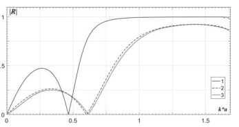
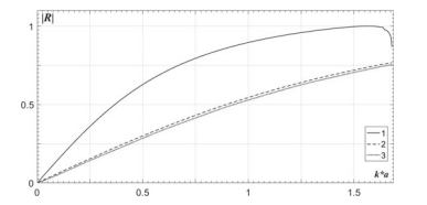
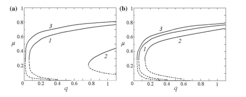
Let us perform a numerical analysis of the problems considered above, on example of the medium with the longitudinal wave speed $c_{1}=6000 \mathrm{~m} / \mathrm{s}$ (steel), and the ratio of the longitudinal and the transverse wave speeds is $c_{1} / c_{2}=1.87$.
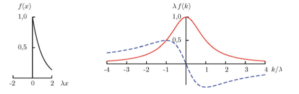
To begin with, let us compare the moduli of reflection and transmission coefficients versus frequency parameter, between the three studied cases, for a single vertical array (see Figs. 2 and 3). With so doing, we assume that the longitudinal wave speed in the problem 2 is equal to the transverse wave speed of the problems 1 and 3. This condition shortens the one-mode frequency interval, whose limit from the right becomes $\pi / 1.87=1.680$, (see Figs. 2 and 3 ). In Figs. $4,5,6,7$ and 8 the comparative numerical analysis of the scalar problems 1 and 3 has been performed for the transverse incident wave. Let us notice that for all cases the filtration interval can be seen in the upper part of the one-mode frequency range. It is shown that lines 2 and 3 in Figs. 2 and 3, related to the scalar problems, are practically coinciding that takes place even for $N=10$ cracks in each vertical array. It should also be noted that line 1 related to the elastic problem, shows a significant domination of the filtration property, when compared with both infinite and finite scalar problems. Let us also notice that for two vertical arrays in the elastic problem a perfect filtration takes place for $a k \geq 0.7$, but for one vertical row this property is valid only for $a k \geq 1.5$; this also confirms the evident property that with the growth of the vertical rows the filtration becomes stronger.
Let us pass to the analysis of the grid size to the precision of the obtained results. It is stated that in the case of a single obstacle it is sufficient to take 10 grid nodes per each wavelength, to provide reliable results. With so doing, for the frequency $0.16 \mathrm{MHz}$ in this formulation the wavelength is $3.75 \mathrm{~cm}$, hence on the obstacle of the length $1.5 \mathrm{~cm}$ it is sufficient to take only 5 nodes. However, the complex geometry of the diffraction lattice requires greater number of nodes. It can be seen from Fig. 4 , which represents the results for the array of 10 vertical rows, each containing 10 obstacles, that with 10 nodes over each obstacle the calculations are correct only in the low-frequency case (for $k^{*} a<1$ ).
物理代写|理论力学代写theoretical mechanics代考|The Propagation of High-Frequency Shear Elastic Waves
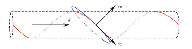
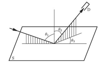
The features of the formation and propagation of forms of an elastic shear wave, concatenated with a canonical (rectangular, periodic in section) protrusions of surfaces each with the other one in elastic isotropic half-spaces (Fig. 7) is investigated [17]. The connection of two half-spaces with surface canonical protrusions is modeled as a composite waveguide consisting of periodically, longitudinally inhomogeneous embedded inner layer in two homogeneous half-spaces.
It is shown from the formation of half-spaces with protrusions, that for the convenience of the mathematical boundary value problem, the coordinate plane yoz
(coordinate plane $x=0$ ) is allocated on one of lateral surfaces of the protrusion contact of the half-spaces $\Omega_{1}{x ; y}$ and $\Omega_{2}{x ; y}$, and the coordinate axis $o z$ is parallel to the forming of these projections. The canonicity of projections (the forms of pins and their linear dimensions) allows us to provide the full mechanical contact along the entire line of contact of half-spaces.
By input of virtual cross-sections, in fact a three-layer waveguide is formed from two homogeneous half-spaces and virtually separated longitudinally inhomogeneous (piecewise-homogeneous) layer of periodically distributed cells of protrusions pairs $\Omega_{1 n}{x ; y}$ and $\Omega_{2 n}{x ; y}$. The mathematical boundary problem on the propagation of normal wave signal (SH) of elastic shear is formulated from the equations of the corresponding homogeneous half-spaces and their respective protrusions:
To study the filtration properties of the metamaterials, let us consider the normal incidence of a plane longitudinal wave, propagating in an unbounded medium $p^{i n c}=$ $\mathrm{e}^{i k x_{1}}$, on a doubly-periodic system of finite number $M(>2)$ of identical vertical arrays, which are finite or infinite along $x_{2}$ and infinite in the direction $x_{3}$. Each of them is an ordinary periodic system of coplanar linear cracks located at $x=0, d, 2 d, \ldots,(M-$ 1)d. In the infinite case, under the natural symmetry, the problem is reduced to the consideration of a plane waveguide of the width $2 a$, which includes $M$ cracks (Fig. 1). For the finite case it is necessary to solve the corresponding boundary integral equation over all available contours of the crack system.
It is assumed that with the normal wave incidence $\mathrm{e}^{i\left(k_{1} x_{1}-\omega t\right)}$ there is a regime of one-mode propagation at $k_{1} a<\pi$, where $k_{1}$-the wave number of the longitudinal wave, $2 a$-the period of the system in the vertical direction, $d$-in the horizontal one. The semi-analytical method is used when the distance between the adjacent parallel arrays $d$ and the incident wave length $\lambda=2 \pi / k_{1}$ are such that the condition $\lambda / d \gg$ 1 is satisfied. A comparative analysis of the properties of the scattering parameters is carried out for the three diffraction problems for a finite and infinite periodic system in a scalar formulation, as well as for an infinite periodic system under the conditions of the plane problem of the elasticity theory.
物理代写|理论力学代写theoretical mechanics代考|Infinite Periodic System. Anti-plane Problem
The solution for elastic problems with infinite periodic arrays of cracks, in the antiplane formulation is presented in $[5,7,15]$. Omitting some routine transformations, the problem can be reduced to the following system of $M$ integral equations regarding the unknown functions $g^{s}(y) ;|y|<b ; s=1, \ldots, M,[8]$ : $\frac{1}{2 a} \int_{-b}^{b} g^{\prime}(t)\left{\frac{1}{2}-\frac{K(y-t)}{i k_{2}}\right} d t+\frac{e^{k_{1} d d}}{4 a} \int_{-b}^{b} g^{2}(t) d t+\frac{e^{2 k k_{2} d}}{4 a} \int_{-b}^{b} g^{3}(t) d t+\ldots+\frac{e^{u k_{2}(M-1) d}}{4 a} \int_{-b}^{b} g^{M}(t) d t=1$ $\frac{e^{a_{1} d}}{4 a} \int_{-6}^{b} g^{1}(t) d t+\frac{1}{2 a} \int_{-1}^{b} g^{2}(t)\left{\frac{1}{2}-\frac{K(y-t)}{i k_{2}}\right) d t+\frac{e^{k_{2} d}}{4 a} \int_{-+}^{h} g^{3}(t) d t+\ldots+\frac{e^{a_{2}(M-2) d}}{4 a} \int_{-h}^{h} g^{M}(t) d t=e^{u_{2} d}$; $\frac{e^{u_{2} 2 d}}{4 a} \int_{-t}^{b} g^{1}(t) d t+\frac{e^{u_{2} d}}{4 a} \int_{-b}^{b} g^{2}(t) d t+\frac{1}{2 a} \int_{-b}^{b} g^{3}(t)\left{\frac{1}{2}-\frac{K(y-t)}{i k_{2}} \int d t+\ldots+\frac{e^{k_{2}(M-5) d}}{4 a} \int_{-b}^{b} g^{M}(t) d t=e^{k_{2} 2 d} ;\right.$ where the kernel has the following form: $K(y)=\sum_{n=1}^{\infty} r_{n} \cos \left(a_{n} y\right), r_{n}=$ $\sqrt{(\pi n / a)^{2}-k_{2}^{2}}, a_{n}=\pi n / a, k_{2}$-the wave number of the incident transverse wave. As mentioned for some aspects of the proposed semi-analytical method [16, 17], it is necessary to consider the auxiliary integral equation, whose kernel $K(y)$ requires a special treatment:$\frac{1}{2 a} \int_{-b}^{b} h(\eta) K(y-\eta) d \eta=1, K(y)=\sum_{n=1}^{\infty} r_{n} \cos \left(a_{n} y\right), \quad|y|<b .$
物理代写|理论力学代写theoretical mechanics代考|Basic Linear Relations of Electro Elasticity
In the future, we will consider only electroacoustic interaction in piezoelectric media, where the complete system of quasistatic equations can be conveniently represented as $$ c_{i j k m} \frac{\partial^{2} u_{k}^{(n)}}{\partial x_{i} \partial x_{m}}+e_{i j m} \frac{\partial^{2} \varphi_{n}}{\partial x_{i} \partial x_{m}}=\rho_{n} \frac{\partial^{2} u_{j}^{(n)}}{\partial t^{2}} ; e_{i j m} \frac{\partial^{2} u_{j}^{(n)}}{\partial x_{i} \partial x_{m}}-\varepsilon_{i m} \frac{\partial^{2} \varphi_{n}}{\partial x_{i} \partial x_{m}}=0 . $$ in which the physicomechanical characteristics of the material form the tensors describing a specific anisotropy of the piezoelectric material $\left{\left(\hat{c}{i j n k}\right){6 \times 6} ;\left(\hat{e}{i j m}\right){3 \times 6} ;\left(\hat{e}{m i j}\right){6 \times 3} ;\left(\hat{\varepsilon}{n k}\right){3 \times 3}\right}_{9 \times 9}$, and determine the structural composition of the coupled electroelastic wave field $\left{u_{i}\left(x_{k}, t\right) ; \varphi\left(x_{k}, t\right)\right}$.
Formally, the role of the conjugation conditions of mechanical fields in the adjoining electro- (magneto-thermo-) elastic media is played by the conditions of continuity of mechanical stresses $\sigma_{i j}^{(m)}$ and elastic displacements $u_{k}^{(m)}$ at the media interface $\Sigma_{m}\left(x_{i}\right)$ $$ \left.\left(\sigma_{i j}^{(1)}-\sigma_{i j}^{(2)}\right) \cdot n_{j}\right|{\Sigma{m}\left(x_{i}\right)}=0 ;\left.\quad u_{k}^{(1)}\right|{\Sigma{w}\left(x_{i}\right)}=\left.u_{k}^{(2)}\right|{\Sigma{w}\left(x_{i}\right)} $$ In electro-elastic media, the conjugacy conditions at the interface of the media are represented as continuity of the tangential components of the electric field strength and normal components of the electric displacements in the adjacent media. In the media interface $\Sigma_{m}\left(x_{i}\right)$, these conditions are written as $$ \left.\left(D_{j}^{(1)}-D_{j}^{(2)}\right) \cdot n_{j}\right|{\Sigma{w}\left(x_{i}\right)}=0 ;\left.\quad \varphi^{(1)}\right|{\Sigma{m}\left(x_{i}\right)}=\left.\varphi^{(2)}\right|{\Sigma{m}\left(x_{i}\right)^{0}} $$ In the problems of electro elasticity (magneto elasticity), the vacuum is also considered as an interacting “medium”, on the outer surfaces of the waveguide. In these cases, the conditions of mechanically open borders are written as $$ \left.\sigma_{i j}^{(1)} \cdot n_{j}\right|{\Sigma{0}\left(x_{i}\right)}=0 . $$ In the case of a rigidly clamped outer surface of the waveguide, we will have the fixing conditions for elastic displacements $$ \left.u_{k}^{(1)}\right|{\Sigma{0}\left(x_{i}\right)}=0 . $$
物理代写|理论力学代写theoretical mechanics代考|The Connection of Two Piezoelectric Layers
When the roughness surfaces of two bodies are joined with the piezoelectric glue (Fig. 1), a near-surface thin non-uniform three-layer with mixed physico mechanical properties is formed $[14,15]$. Take into account a thinness of the near-surface zone,
the piecewise-homogeneous three-layer is modeled as an internal meta-surface of a two-layer waveguide, with unique physical and geometric characteristics (Fig. 1). The thickness of the adhesive layer is also small compared to the effective thickness of the adjacent layers. In studies of the propagation of the wave signal electroactive antiplane deformation, in the internal adhesive gap of variable width $\Omega_{3}=\left{|x|<\infty, h_{2}(x) \leq y \leq h_{1}(x),|z|<\infty\right}$, as well as in each half space $\Omega_{1}=\left{|x|<\infty, h_{1}(x) \leq y<\infty,|z|<\infty\right}$ and $\Omega_{2}=\left{|x|<\infty,-\infty<y \leq h_{2}(x),|z|<\infty\right}$ quasistatic equations of electroactive antiplane deformation are solved $$ \begin{gathered} c_{44}^{(m)} \frac{\partial^{2} \mathrm{w}{m}}{\partial x^{2}}+e{15}^{(m)} \frac{\partial^{2} \varphi_{m}}{\partial x^{2}}+\frac{\partial \sigma_{y z}^{(m)}}{\partial y}=\rho_{m} \frac{\partial^{2} \mathrm{w}{m}}{\partial t^{2}} ; \ e{15}^{(m)} \frac{\partial^{2} \mathrm{w}{m}}{\partial x^{2}}-\varepsilon{11}^{(m)} \frac{\partial^{2} \varphi_{m}}{\partial x^{2}}+\frac{\partial D_{y}^{(m)}}{\partial y}=0 \end{gathered} $$ Taking into account the effective thickness of the adjacent layers, the solutions of Eqs. (3.1) and (3.2) in each half space have the following form $$ \begin{gathered} \mathrm{w}{n}(x, y, t)=W{0 n} \exp \left[(-1)^{n} \alpha_{n} k y\right] \cdot \exp [i(k x-\omega t)] \ \varphi_{n}(x, y, t)=\left{\begin{array}{l} \Phi_{0 n} \exp \left[(-1)^{n} k y\right] \ +\left(e_{n} \backslash \varepsilon_{n}\right) \cdot W_{0 n} \exp \left[(-1)^{n} \alpha_{n} k y\right] \end{array}\right} \cdot \exp [i(k x-\omega t)] \end{gathered} $$ The function of the distribution of the wave field is chosen so that it simply and completely (without loss of physical phenomena) describes the nature of the change of the desired quantities on surfaces and along the thickness of the adhesive layer.
物理代写|理论力学代写theoretical mechanics代考|Smoothing the Roughness of the Surfaces
Smoothing the roughness of the surfaces of the piezoelectric layer by pouring different materials (Fig. 2), in the near-surface zones, thin non-uniform double layers with mixed physical and mechanical properties are formed $[16,18,19]$. Different fills lead to the formation of heterogeneous electromechanical meta-surfaces of the piezoelectric base layer.
Let us assume that the waveguide surface irregularities $y=h_{+}(x)$ are filled to the level $y=h_{0}\left(1+\gamma_{+}\right)$with a good dielectric, and the waveguide’s surface irregularities $y=h_{-}(x)$ are filled to the level $y=-h_{0}\left(1+\gamma_{-}\right)$with a good electrical conductor. Here $\gamma_{\pm} \ll 1$ are the heights of the profiles of irregularities and $h_{0}$ is a half of the base thickness of the homogeneous piezoelectric layer. So we have a composite waveguide, which consists of five layers:
the base layer $\Omega_{0}{x, y}$ of a constant thickness $-h_{0}\left(1-\gamma_{-}\right) \leq y \leq h_{0}\left(1-\gamma_{+}\right)$
an electrically conductive layer $\Omega_{-}^{c}{x, y}$ of thickness $\xi_{c}(x)=$ $\left|h_{0}\left(1+\gamma_{-}\right)+h_{-}(x)\right|$
nonhomogeneous piezoelectric thin layer $\Omega_{-}^{p}{x, y}$ of thickness $\xi_{p-}(x)=$ $\left|-h_{0}\left(1-\gamma_{-}\right)-h_{-}(x)\right|$
nonhomogeneous piezoelectric thin layer $\Omega_{+}^{p}{x, y}$ of thickness $\xi_{p+}(x)=$ $\left|h_{+}(x)-h_{0}\left(1-\gamma_{+}\right)\right|$
a dielectric thin layer $\Omega_{+}^{d}{x, y}$ of thickness $\xi_{d}(x)=h_{0}\left(1+\gamma_{+}\right)-h_{+}(x)$. Thus, near the surface area $y=h_{-}(x)$ we have a composite layer, which consists of transversely inhomogeneous piezoelectric and homogeneous, perfectly conducting materials. The same way, near the surface area $y=h_{+}(x)$ we have a composite layer, which consists of homogeneous dielectric and transversely inhomogeneous piezoelectric materials. The homogeneous piezoelectric waveguide with filled surface irregularities is modeled as a multilayer waveguide made of different materials.
物理代写|理论力学代写theoretical mechanics代考|The Study of the Problem in the Local Formulation
Let a circular monochromatic high-frequency wave fall from the point $x_{0}$ of the infinite elastic plane to the boundary contour $l$ of an obstacle or a system of obstacles in it. The wave is generated by the force $Q e^{i \omega t}$ located at point $x_{0}$, where $\omega$ is the oscillation frequency. In this case, the displacements at the point $y$ of the elastic plane are determined by the Kupradze matrix [7].
The aim is to study the amplitude characteristics of the scattered field by the contours of obstacles in the through-transmitted elastic wave.
In the directions $\mathbf{q}{1}$ and $\mathbf{q}{2}$ we have asymptotic representations of the amplitudes of displacements in the incident wave $$ \begin{gathered} \mathbf{u}{\mathbf{q}}^{(p)}(y)=\frac{Q{\mathrm{q}}}{4 \mu} \mathbf{q} i \frac{k_{p}^{2}}{k_{s}^{2}} \sqrt{\frac{2}{\pi k_{p}}} \mathrm{e}^{-i \frac{\pi}{4}} \frac{\mathrm{e}^{i k_{p} R_{0}}}{\sqrt{R_{0}}}\left[1+\mathrm{O}\left(\left(\frac{1}{k_{p} R_{0}}\right)\right)\right], \quad Q_{\mathrm{q}}=(\mathrm{Q}, \mathrm{q}), \ \mathbf{u}{\mathrm{q}{1}}^{(s)}(y)=\frac{Q_{\mathrm{q}{1}}}{4 \mu} \mathbf{q}{1} i \sqrt{\frac{2}{\pi k_{s}}} \mathrm{e}^{-i \frac{\pi}{4}} \frac{\mathrm{e}^{i k_{s} R_{0}}}{\sqrt{R_{0}}}\left[1+\mathrm{O}\left(\frac{1}{k_{s} R_{0}}\right)\right], \quad Q_{\mathbf{q}{1}}=\left(\mathrm{Q}, \mathrm{q}{1}\right) . \end{gathered} $$ Here the tangential direction $\mathbf{q}{1}$ is perpendicular to $\mathbf{q}{\mathbf{1}} Q_{\mathbf{q}}$ and $Q_{\mathbf{q}{1}}$ are the projections of the force $\mathbf{Q}$ on the directions $\mathbf{q}$ and $\mathbf{q}{1}$. Here $\rho$ is the mass density, $\lambda, \mu$ are the Lamè coefficients, $k_{p}=\omega / c_{p}, k_{s}=\omega / c_{s}, c_{p}$ and $c_{S}$ are the wave numbers and the velocities of the longitudinal and transverse waves. The components of the displacement vector in the reflected wave from the free boundary contour at the point $x$ of the elastic plane are determined by the following integral [8] $$ \begin{gathered} u_{k}(x)=\int_{l} \mathbf{T}{y}\left[\mathbf{U}^{(k)}(y, x)\right] \cdot \mathbf{u}(y) d l, \quad k=1,2 \ \mathbf{T}{y}\left[\mathbf{U}^{(k)}(y, x)\right]=2 \mu \frac{\partial \mathbf{U}^{(k)}}{\partial n}+\lambda \mathbf{n} \operatorname{div}\left(\mathbf{U}^{(k)}\right)+\mu\left(\mathbf{n} \times \operatorname{rot}\left(\mathbf{U}^{(k)}\right)\right) \end{gathered} $$ where the Kupradze matrix $\mathbf{U}^{(k)}(y, x)$ is obtained from the matrix $\mathbf{U}^{(k)}\left(y, x_{0}\right)$ by replacing $x_{0}$ by $x$ and $R_{0}$ by $R=|y-x|$. $\mathbf{T}_{y}$ is the force vector at the point $y$, $\mathbf{u}(y)$ is the vector of the total displacement field on the boundary surface, $\mathbf{n}$ is the outer unit normal to the contour $l$, directed toward the elastic medium.
物理代写|理论力学代写theoretical mechanics代考|Two-Fold Reflection of Elastic Waves on the Plane
This section is devoted to the development of the ray diffraction theory with respect to arbitrary (nonconvex) smooth two-dimensional obstacles in an elastic medium. Double re-reflection of the high-frequency wave, taking into account possible transformations, can be formed both within the contour of one obstacle (Fig. 1) and two different obstacles (Fig. 2). Numerical investigation of the problems of highfrequency scattering of elastic waves is considerably complex if the wavelength is much smaller than the average size of the scatterer. There are some known numerical methods-the finite element method, the method of boundary elements, all require in this case a large number of nodes on the grid. This leads to instability of the calculation. To calculate the displacement amplitude in a multiply re-reflected wave, it is possible to use the Keller geometric theory of diffraction (GTD) [11], based on the use of divergence coefficients, which is rather cumbersome. If we investigate the problem of the reflection of a high-frequency wave from an obstacle contour in an elastic medium with various possible wave transformations of an arbitrary finite number of times $N$, then it is more convenient to start from the estimate of the $N$-fold multiple diffraction integral by the multidimensional stationary phase method. The basis for the investigation of the general case of an arbitrary number of re-reflections is the solution of the problem of double reflection (Figs. 1 and 2), to which we turn. The direct usage of the integral representation (3) over the entire “light” zone for reflected waves is impossible [9], since it does not describe multiply reflected waves. If one substitutes to the Green’s formula (3) the solution of [12] for local problems (8) and $(10$ ) and as the primary field takes the total field $u(y)$, then the integral formula (3) gives only a single-reflected wave. A doubly reflected wave is obtained only when the values of $u(y)$ include both the primary field and its single reflection. To solve the problem of double re-reflection, we start from the modification [9] of the integral formula (3). Following this modification, the doubly reflected waves will be found by integrating along the neighborhood $l_{2}^{}$ of the second mirror reflection point $y_{2}^{}$ the rays obtained upon single reflection from the neighborhood $l_{1}^{}$ of the first mirror reflection point $y_{1}^{}$. Such a modification means that when finding the leading term of the asymptotics of the double diffraction integral, we stay within the framework of the calculation of the displacement amplitude in a doubly reflected wave in accordance with the GTD.
物理代写|理论力学代写theoretical mechanics代考|Multiple Reflections with All Possible Transformations
The geometry of the boundary contours of the obstacles in the elastic medium and their arrangement can form such trajectories of the rays $x_{0}-y_{1}^{}-y_{2}^{}-\cdots-y_{N}^{}-x_{N+1}$ which lead to any possible sequence of reflections and wave transformations at the points of specular reflection. Suppose that for any $N$ times re-reflected ray, in a certain order, $p-p$ and $s-s$ reflections have been realized at the mirror reflection points $y_{1}^{}, y_{2}^{}, \ldots, y_{N-1}^{}, y_{N}^{}$, respectively $N_{1}$ and $N_{3}$ times, and $p-s$, and $s-p$, transformations-respectively $N_{2}$ and $N_{4}$ times. At the receiving point $x_{N+1}$, both the longitudinal wave $u\left(x_{N+1}\right)=u_{r}^{(p)}\left(x_{N+1}\right)$ and the transverse one $u\left(x_{N+1}\right)=u_{\theta}^{(s)}\left(x_{N+1}\right)$ may be received. In this case, the amplitude of the radial or tangential displacement of the $N$ times reflected ray at the point $x_{N+1}$ relatively the local polar coordinate system $r, \theta$ at the point $y_{N}^{}$ of the boundary contour of the obstacle is represented by the multiple Kirchhoff integral, which is formed according to the same laws as the diffraction integral (11), by taking into account reflections and transformations of the propagating ray at the points of mirror reflection: $u_{r}^{(p)}\left(x_{N+1}\right)=B(-1)^{N} \mathrm{e}^{-i \frac{\pi}{4}}\left(\frac{k_{p}}{2 \pi}\right)^{\frac{N_{1}+N_{2}}{2}}\left(\frac{k_{s}}{2 \pi}\right)^{\frac{N_{3}+N_{4}}{2}} \frac{1}{\sqrt{L_{0}}} \prod_{n=1}^{N} \frac{\cos \gamma_{n}^{(2)}}{\sqrt{L_{n}}} V\left(y_{n}^{}\right)$ $\times \int_{l_{N}} \int_{l_{N-1}} \ldots \int_{l_{2}^{}} \int_{l_{i}^{}} \mathrm{e}^{i k_{P \psi}} d l_{N} d l_{N-1} \ldots d l_{2} d l_{1}$ $\varphi=k_{p}^{-1}\left(k_{1}\left|x_{0}-y_{1}\right|+\sum_{n=1}^{N-1} k_{n}\left|y_{n}-y_{n+1}\right|+k_{N}\left|y_{N}-x_{N+1}\right|\right)$ $L_{0}=\left|x_{0}-y_{1}^{}\right|, L_{n}=\left|y_{n}^{}-y_{n+1}^{}\right|, L_{N}=\left|y_{N}^{*}-x_{N+1}\right|, \quad n=1,2, \ldots, N-1 .$
物理代写|理论力学代写theoretical mechanics代考|Effect of Thickness on the Magnitude of Spontaneous
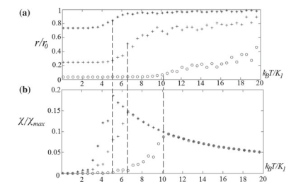
To describe properties of the ferroelectric films and to study of ordering effects we use a three-dimensional lattice model (Fig. 10), consisting of $N_{1}, N_{2}$ and $N_{3}$ nodes along the respective axes of the Cartesian coordinate system. The position of the lattice node is characterized by the set of three numbers $\vec{n}=\left(n_{1}, n_{2}, n_{3}\right)$.
In this paper, the interaction energy of dipoles is described by a potential that takes into account the energy of orientation interactions (as in the classical Ising model) and the additional term representing the Lennard-Jones potential: $$ H=H_{o r}+\sum_{\vec{n}, \vec{m}} \varepsilon\left(\frac{r_{0}^{12}}{r_{\vec{n}, \vec{m}}^{12}}-\frac{2 r_{0}^{6}}{r_{\vec{n}, \vec{m}}^{6}}\right), $$ where $\varepsilon$ is the potential well depth of the Lennard-Jones potential, $r_{i, j}, j$ is the distance between the dipoles, $r_{0}$ is average distance in the absence of orientation interactions.
The second term of Eq. (14) does not depend on the temperature and the polarization, in contrast to the first term.
When the polarization decreases, therefore, we must take into account that the distance between the dipoles changes in transverse dimensions $N_{2}$ and $N_{3}$ of film. The potential of orientation interactions $H_{o r}$ is represented by the formula: $$ \begin{aligned} H_{o r}=&-\sum_{\vec{n}} K_{1} S_{n_{1}, n_{2}, n_{3}} S_{n_{1}-1, n_{2}, n_{3}}-\sum_{\vec{n}} K_{2} \frac{r_{0}^{3}}{r^{3}} S_{n_{1}, n_{2}, n_{3}} S_{n_{1}, n_{2}-1, n_{3}} \ &-\sum_{\vec{n}} K_{2} \frac{r_{0}^{3}}{r^{3}} S_{n_{1}, n_{2}, n_{3}} S_{n_{1}, n_{2}, n_{3}-1}+p \sum_{\vec{n}} S_{\vec{n}} E_{d} \end{aligned} $$ where the quantity $S_{-n}$ takes only two values $+1$ and $-1, K_{1}$ is the coefficient of exchange interactions in the longitudinal direction, $p$ is the dipole moment, $K_{2}$ is the constant of exchange interactions between the dipoles in the transverse direction, $E_{d}$ is the projection of the vector of the depolarizing field strength on the direction $N_{1}$.
物理代写|理论力学代写theoretical mechanics代考|Modeling of Geometric and Optical Properties
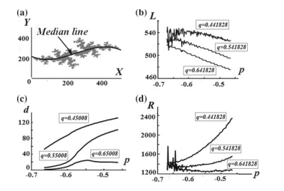
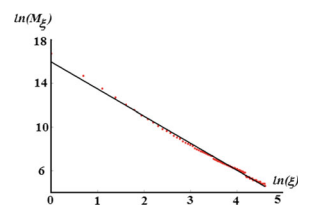
The solution of the problem of creating surfaces with certain properties is necessary both for stable functioning of products and technological control of the surface quality of such products [33]. The use of the fractal approach to describe structural in homogeneities, as well as the justification of general regularities, is one of the modern scientific trends in the surface physics and the chemistry of solids. At present, various mathematical models of fractals (Sierpinski rug, Mandelbrot set), describe well the real imperfections (Brownian) surfaces of metal layers, dielectric layers [34], semiconductor surfaces [35] those have defects of a symmetric type [36, 37]. However, when examining the surface of polymer coatings of metal sheet, the detected defects are anisotropic (Fig. 16a); therefore, these models cannot be used to describe their structure. In this paper, the three-dimensional anisotropic model based on the Julia set will be used to construct a fractal model of the surface. Algorithm of creating of the fractals To construct fractal surfaces of the extured polymer coating of sheet metal (Fig. 16a, b), the following algorithm was used:
The area in which the fractal is created is divided into $1000 \times 1000$ rectangles. Each rectangle is characterized by the coordinates $\left(X_{r, s}, Y_{r, s}\right)$ of its center.
A sequence is defined by the recurrence formula [38]. $$ Z_{r, s}^{(n)}=\left(Z_{r, s}^{(n-1)}\right)^{2}+p+i q, $$ where values $p$ and $q$ are parameters of the fractal function (22). The first term of the sequence is defined as $$ Z_{r, s}^{(1)}=X_{r, s}+i Y_{r, s} $$
The value of $H$ is select inversely to the rate of increase of the modulus of the sequence term (1). $H$ is equal to the smallest number of the sequence term, when $\left|z_{i}\right|>Q$. In our calculations, we assumed that the value is $Q=10^{6}$. The examples of fractal functions obtained are shown in Fig. 16c, d.
In an infinite two-dimensional elastic medium there is an array of obstacles. The obstacles can be of two types: absolutely solid and voids. In the array of obstacles, a pulse is introduced with a tonal filling by several periods of a planar high-frequency, monochromatic longitudinal or transverse elastic wave, and in a certain region of the elastic medium, a transmitted wave with any possible reflections (longitudinal wave to longitudinal one, transverse wave to transverse one) and transformations (longitudinal wave to transverse one, transverse wave to longitudinal one).
The aim of the study is to obtain analytical expressions for displacements in the transmitted longitudinal or transverse wave.
The structure of the input pulse makes it possible to investigate the problem in the regime of harmonic oscillations. The incident plane elastic wave is replaced by a set of point sources of cylindrical waves. Each cylindrical wave propagating in an angle with a vertex in the source directed toward the obstacles and a contracted semi-circle is replaced by a system of corresponding radial propagation rays of the elastic wave. Thus, the problem is reduced to a problem of short-wave diffraction of elastic waves in a local formulation. The total field in the region of reception of propagating elastic waves is composed of rays transmitted through a system of obstacles, which can be of the three types: rays transmitted through the obstacle system without diffraction; rays reflected from the system once or a finite number of times.