计算方法代写

分类：计算方法代写

数学代写|计算方法代写computational method代考|Equations of linear elasticity – strong form

Posted on 2022年5月17日2022年5月17日 by statistics-lab

如果你也在怎样代写计算方法computational method这个学科遇到相关的难题，请随时右上角联系我们的24/7代写客服。

计算方法是基于计算机的方法，用于数值解决描述物理现象的数学模型。计算研究方法利用计算方面的新进展，如算法、模型、模拟和系统，以了解复杂的社会、生物、技术和无尽的其他模式和行为。

statistics-lab™ 为您的留学生涯保驾护航在代写计算方法computational method方面已经树立了自己的口碑, 保证靠谱, 高质且原创的统计Statistics代写服务。我们的专家在代写计算方法computational method代写方面经验极为丰富，各种代写计算方法computational method相关的作业也就用不着说。

我们提供的计算方法computational method及其相关学科的代写，服务范围广, 其中包括但不限于:

Statistical Inference 统计推断
Statistical Computing 统计计算
Advanced Probability Theory 高等概率论
Advanced Mathematical Statistics 高等数理统计学
(Generalized) Linear Models 广义线性模型
Statistical Machine Learning 统计机器学习
Longitudinal Data Analysis 纵向数据分析
Foundations of Data Science 数据科学基础

数学代写|计算方法代写computational method代考|Equations of linear elasticity – strong form

数学代写|计算方法代写computational method代考|Strain-displacement relationships

Mathematical problems of linear elasticity belong in the category of vector elliptic boundary value problems. The unknown functions are the components of the displacement vector. In Cartesian coordinates the displacement vector is:
$$
\begin{aligned}
\mathbf{u} & \stackrel{\text { def }}{ }=u_{x}(x, y, z) \mathbf{e}{x}+u{y}(x, y, z) \mathbf{e}{y}+u{z}(x, y, z) \mathbf{e}{z} \ & \equiv\left{u{x}(x, y, z) u_{y}(x, y, z) u_{z}(x, y, z)\right}^{T} \
& \equiv u_{i}\left(x_{j}\right)
\end{aligned}
$$
where $\mathbf{e}{x}, \mathbf{e}{y}, \mathbf{e}_{z}$ are the Cartesian basis vectors.
The formulation of problems of linear elasticity is based on three fundamental relationships: the strain-displacement equations, the stress-strain relationships and the equilibrium equations.

Strain-displacement relationships. We introduce the infinitesimal strain-displacement relationships here. A detailed derivation of these relationships is presented in Section 9.2.1. By definition, the infinitesimal normal strain components are:
$$
\epsilon_{x} \equiv \epsilon_{x x} \stackrel{\text { def }}{=} \frac{\partial u_{x}}{\partial x} \quad \epsilon_{y} \equiv \epsilon_{y y} \stackrel{\text { def }}{=} \frac{\partial u_{y}}{\partial y} \quad \epsilon_{z} \equiv \epsilon_{z z} \stackrel{\text { def }}{=} \frac{\partial u_{z}}{\partial z}
$$
and the shear strain components are:
$$
\begin{aligned}
&\left.\epsilon_{x y}=\epsilon_{y x} \equiv \frac{\gamma_{x y}}{2} \stackrel{\operatorname{def} 1}{=} \frac{\partial u_{x}}{\partial y}+\frac{\partial u_{y}}{\partial x}\right) \
&\epsilon_{y z}=\epsilon_{z y} \equiv \frac{\gamma_{y z}}{2} \stackrel{\operatorname{det} 1}{=}\left(\frac{\partial u_{y}}{\partial z}+\frac{\partial u_{z}}{\partial y}\right) \
&\epsilon_{z x}=\epsilon_{x z} \equiv \frac{\gamma_{z x}}{2} \stackrel{\text { def }}{=} \frac{1}{2}\left(\frac{\partial u_{z}}{\partial x}+\frac{\partial u_{x}}{\partial z}\right)
\end{aligned}
$$

where $\gamma_{x y}, \gamma_{y z}, \gamma_{z x}$ are called the engineering shear strain components. In index notation, the infinitesimal strain at a point is characterized by the strain tensor
$$
\epsilon_{i j} \stackrel{\text { def }}{=} \frac{1}{2}\left(u_{i, j}+u_{j, i}\right) .
$$

Stress-strain relationships Mechanical stress is defined as force per unit area $\left(\mathrm{N} / \mathrm{m}^{2} \equiv \mathrm{Pa}\right)$. Since one Pascal (Pa) is a very small stress, the usual unit of mechanical stress is the Megapascal (MPa) which can be understood to mean either $10^{6} \mathrm{~N} / \mathrm{m}^{2}$ or $1 \mathrm{~N} / \mathrm{mm}^{2}$.
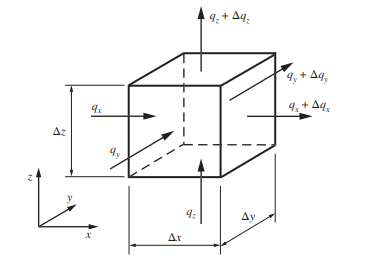
The usual notation for stress components is illustrated on an infinitesimal volume element shown in Fig. 2.7. The indexing rules are as follows: Faces to which the positive $x, y, z$ axes are normal are called positive faces, the opposite faces are called negative faces. The normal stress components are denoted by $\sigma$, the shear stresses components by $\tau$. The normal stress components are assigned one subscript only, since the orientation of the face and the direction of the stress component are the same. For example, $\sigma_{x}$ is the stress component acting on the faces to which the $x$-axis is normal and the stress component is acting in the positive (resp. negative) coordinate direction on the positive (resp. negative) face. For the shear stresses, the first index refers to the coordinate direction of the normal to the face on which the shear stress is acting. The second index refers to the direction in which the shear stress component is acting.
On a positive (resp. negative) face the positive stress components are oriented in the positive (resp. negative) coordinate directions. The reason for this is that if we subdivide a solid body into infinitesimal hexahedral volume elements, similar to the element shown in Fig. 2.7, then each negative face will be coincident with a positive face. By the action-reaction principle, the forces acting on those faces must have equal absolute value and opposite sign. In index notation $\sigma_{11} \equiv \sigma_{x}, \sigma_{12} \equiv \sigma_{x y} \equiv \tau_{x y}$, etc.

数学代写|计算方法代写computational method代考|Boundary and initial conditions

As in the case of heat conduction, we will consider three kinds of boundary conditions: prescribed displacements, prescribed tractions and spring boundary conditions. Tractions are forces per unit area acting on the boundary. Prescribed displacements and tractions are often specified in a normal-tangent reference frame.

Prescribed displacement. One or more components of the displacement vector is prescribed on all or part of the boundary. This is called a kinematic boundary condition.
Prescribed traction. One or more components of the traction vector is prescribed on all or part of the boundary. The definition of traction vector is given in Appendix K.1.
Linear spring. A linear relationship is prescribed between the traction and displacement vector components. The general form of this relationship is:
$$
T_{i}=c_{i j}\left(d_{j}-u_{j}\right)
$$
where $T_{i}$ is the traction vector, $c_{i j}$ is a positive-definite matrix that represents the distributed spring coefficients; $d_{j}$ is a prescribed function that represents displacement imposed on the spring and $u_{j}$ is the (unknown) displacement vector function on the boundary. The spring coefficients $c_{i j}$ (in $\mathrm{N} / \mathrm{m}^{3}$ units) may be functions of the position $x_{k}$ but are independent of the displacement $u_{i}$. This is called a “Winkler spring ${ }^{12}$ “.
A schematic representation of this boundary condition on an infinitesimal boundary surface element is shown in Fig. $2.8$ under the assumption that $c_{i j}$ is a diagonal matrix and therefore three spring coefficients $c_{1} \stackrel{\text { def }}{=} c_{11}, c_{2} \stackrel{\text { def }}{=} c_{22}, c_{3} \stackrel{\text { def }}{=} c_{33}$ characterize the elastic properties of the boundary condition.
Fig. $2.8$ should be interpreted to mean that the imposed displacement $d_{i}$ will cause a differential force $\Delta F_{i}$ to act on the centroid of the surface element. Suspending the summation rule, the magnitude of $\Delta F_{i}$ is
$$
\Delta F_{i}=c_{i} \Delta A\left(d_{i}-u_{i}\right), \quad i=1,2,3
$$
where $u_{i}$ is the displacement of the surface element. The corresponding traction vector is:
$$
T_{i}=\lim {\Delta A \rightarrow 0} \frac{\Delta F{i}}{\Delta A}=c_{i}\left(d_{i}-u_{i}\right), \quad i=1,2,3 .
$$

数学代写|计算方法代写computational method代考|Symmetry, antisymmetry and periodicity

Symmetry and antisymmetry of vectors in two dimensions with respect to the $y$ axis is illustrated in Fig. $2.9$

The definition of symmetry and antisymmetry of vectors in three dimensions is analogous: the corresponding vector components parallel to a plane of symmetry (resp. antisymmetry) have the same absolute value and the same (resp. opposite) sign. The corresponding vector components normal to a plane of symmetry (resp. antisymmetry) have the same absolute value and opposite (resp. same) sign.

In a plane of symmetry the normal displacement and the shearing traction components are zero. In a plane of antisymmetry the normal traction is zero and the in-plane components of the displacement vector are zero.

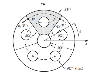
When the solution is periodic on $\Omega$ then a periodic sector of $\Omega$ has at least one periodic boundary segment pair denoted by $\partial \Omega_{p}^{+}$and $\partial \Omega_{p}^{-}$. On corresponding points of a periodic boundary segment pair, $P^{+} \in \partial \Omega_{p}^{+}$and $P^{-} \in \partial \Omega_{p}^{-}$the normal component of the displacement vector and the periodic in-plane components of the displacement vector have the same value. The normal component of the traction vector and the periodic in-plane components of the traction vector have the same absolute value but opposite sign.

Owing to the complexity of three-dimensional problems in elasticity, dimensional reduction is widely used. Various kinds of dimensional reduction are possible in elasticity, such as planar, axisymmetric, shell, plate, beam and bar models. Each of these model types is sufficiently important to have generated a substantial technical literature. In the following models for planar and axially symmetric problems are discussed. Models for beams, plates and shells will be discussed separately.

数学代写|计算方法代写computational method代考|Strain-displacement relationships

线性弹性的数学问题属于向量椭圆边值问题的范畴。未知函数是位移矢量的分量。在笛卡尔坐标中，位移矢量为：
\begin{aligned} \mathbf{u} & \stackrel{\text { def }}{ }=u_{x}(x, y, z) \mathbf{e}{x}+u{y}(x, y, z) \mathbf{e}{y}+u{z}(x, y, z) \mathbf{e}{z} \ & \equiv\left{u{x}(x, y, z) u_{y}(x, y, z) u_{z}(x, y, z)\right}^{T} \ & \equiv u_{i}\left(x_{j}\right) \end{对齐}\begin{aligned} \mathbf{u} & \stackrel{\text { def }}{ }=u_{x}(x, y, z) \mathbf{e}{x}+u{y}(x, y, z) \mathbf{e}{y}+u{z}(x, y, z) \mathbf{e}{z} \ & \equiv\left{u{x}(x, y, z) u_{y}(x, y, z) u_{z}(x, y, z)\right}^{T} \ & \equiv u_{i}\left(x_{j}\right) \end{对齐}
在哪里和X,和是,和和是笛卡尔基向量。
线性弹性问题的表述基于三个基本关系：应变-位移方程、应力-应变关系和平衡方程。

应变-位移关系。我们在这里介绍了无穷小的应变-位移关系。这些关系的详细推导在第 9.2.1 节中介绍。根据定义，无穷小的法向应变分量为：
εX≡εXX= 定义 ∂在X∂Xε是≡ε是是= 定义 ∂在是∂是ε和≡ε和和= 定义 ∂在和∂和
剪应变分量为：
εX是=ε是X≡CX是2=定义⁡1∂在X∂是+∂在是∂X) ε是和=ε和是≡C是和2=这⁡1(∂在是∂和+∂在和∂是) ε和X=εX和≡C和X2= 定义 12(∂在和∂X+∂在X∂和)

在哪里CX是,C是和,C和X称为工程剪应变分量。在指数符号中，一点的无穷小应变由应变张量表征
ε一世j= 定义 12(在一世,j+在j,一世).

应力-应变关系机械应力定义为每单位面积的力(ñ/米2≡磷一种). 由于一个帕斯卡 (Pa) 是非常小的应力，因此机械应力的常用单位是兆帕 (MPa)，可以理解为106 ñ/米2或者1 ñ/米米2.
应力分量的常用符号在图 2.7 所示的一个无穷小体积单元上进行了说明。索引规则如下：X,是,和轴正常的称为正面，相反的面称为负面。法向应力分量表示为σ, 剪应力分量由τ. 法向应力分量仅分配一个下标，因为面的方向和应力分量的方向相同。例如，σX是作用在面的应力分量X- 轴是法线，应力分量在正（或负）面的正（或负）坐标方向上作用。对于剪切应力，第一个指标是指剪切应力作用面的法线坐标方向。第二个指标是指剪切应力分量作用的方向。
在正（或负）面上，正应力分量朝向正（或负）坐标方向。这样做的原因是，如果我们将一个实体细分为无穷小的六面体体积单元，类似于图 2.7 中所示的单元，那么每个负面将与一个正面重合。根据作用-反作用原理，作用在这些面上的力必须具有相等的绝对值和相反的符号。在索引符号中σ11≡σX,σ12≡σX是≡τX是， ETC。

数学代写|计算方法代写computational method代考|Boundary and initial conditions

与热传导的情况一样，我们将考虑三种边界条件：规定位移、规定牵引力和弹簧边界条件。牵引力是作用在边界上的每单位面积的力。规定的位移和牵引力通常在法向切线参考系中指定。

规定的位移。位移矢量的一个或多个分量被规定在全部或部分边界上。这称为运动学边界条件。
规定的牵引力。牵引矢量的一个或多个分量被规定在全部或部分边界上。牵引矢量的定义见附录 K.1。
线性弹簧。在牵引力和位移矢量分量之间规定了线性关系。这种关系的一般形式是：
吨一世=C一世j(dj−在j)
在哪里吨一世是牵引矢量，C一世j是一个正定矩阵，表示分布的弹簧系数；dj是一个规定的函数，表示施加在弹簧上的位移，并且在j是边界上的（未知）位移矢量函数。弹簧系数C一世j（在ñ/米3单位）可能是位置的函数Xķ但与位移无关在一世. 这被称为“温克勒弹簧”12“。
这种边界条件在一个无穷小的边界面单元上的示意图如图 1 所示。2.8在假设C一世j是对角矩阵，因此是三个弹簧系数C1= 定义 C11,C2= 定义 C22,C3= 定义 C33表征边界条件的弹性特性。
如图。2.8应该被解释为意味着施加的位移d一世会产生不同的力ΔF一世作用于面元的质心。暂停求和规则，大小ΔF一世是
ΔF一世=C一世Δ一种(d一世−在一世),一世=1,2,3
在哪里在一世是面元的位移。对应的牵引向量为：
吨一世=林Δ一种→0ΔF一世Δ一种=C一世(d一世−在一世),一世=1,2,3.

数学代写|计算方法代写computational method代考|Symmetry, antisymmetry and periodicity

二维向量的对称性和反对称性是轴如图所示。2.9

三维向量的对称性和反对称性的定义是类似的：平行于对称平面的相应向量分量（分别是反对称）具有相同的绝对值和相同的（或相反的）符号。垂直于对称平面（分别是反对称）的相应矢量分量具有相同的绝对值和相反的（相应的）符号。

在对称平面中，法向位移和剪切牵引分量为零。在反对称平面中，法向牵引力为零，位移矢量的平面内分量为零。

当解决方案是周期性的Ω然后是一个周期性扇区Ω具有至少一个周期性边界段对，表示为∂Ωp+和∂Ωp−. 在周期性边界段对的对应点上，磷+∈∂Ωp+和磷−∈∂Ωp−位移矢量的法向分量和位移矢量的周期性平面内分量具有相同的值。牵引矢量的法向分量和牵引矢量的周期性平面内分量具有相同的绝对值但符号相反。

由于弹性中三维问题的复杂性，降维被广泛使用。弹性的各种降维是可能的，例如平面、轴对称、壳、板、梁和杆模型。这些模型类型中的每一种都非常重要，足以产生大量的技术文献。下面讨论平面和轴对称问题的模型。梁、板和壳的模型将单独讨论。

数学代写|计算方法代写computational method代考请认准statistics-lab™

统计代写请认准statistics-lab™. statistics-lab™为您的留学生涯保驾护航。

金融工程代写

金融工程是使用数学技术来解决金融问题。金融工程使用计算机科学、统计学、经济学和应用数学领域的工具和知识来解决当前的金融问题，以及设计新的和创新的金融产品。

非参数统计代写

非参数统计指的是一种统计方法，其中不假设数据来自于由少数参数决定的规定模型；这种模型的例子包括正态分布模型和线性回归模型。

广义线性模型代考

广义线性模型（GLM）归属统计学领域，是一种应用灵活的线性回归模型。该模型允许因变量的偏差分布有除了正态分布之外的其它分布。

术语广义线性模型（GLM）通常是指给定连续和/或分类预测因素的连续响应变量的常规线性回归模型。它包括多元线性回归，以及方差分析和方差分析（仅含固定效应）。

有限元方法代写

有限元方法（FEM）是一种流行的方法，用于数值解决工程和数学建模中出现的微分方程。典型的问题领域包括结构分析、传热、流体流动、质量运输和电磁势等传统领域。

有限元是一种通用的数值方法，用于解决两个或三个空间变量的偏微分方程（即一些边界值问题）。为了解决一个问题，有限元将一个大系统细分为更小、更简单的部分，称为有限元。这是通过在空间维度上的特定空间离散化来实现的，它是通过构建对象的网格来实现的：用于求解的数值域，它有有限数量的点。边界值问题的有限元方法表述最终导致一个代数方程组。该方法在域上对未知函数进行逼近。[1] 然后将模拟这些有限元的简单方程组合成一个更大的方程系统，以模拟整个问题。然后，有限元通过变化微积分使相关的误差函数最小化来逼近一个解决方案。

tatistics-lab作为专业的留学生服务机构，多年来已为美国、英国、加拿大、澳洲等留学热门地的学生提供专业的学术服务，包括但不限于Essay代写，Assignment代写，Dissertation代写，Report代写，小组作业代写，Proposal代写，Paper代写，Presentation代写，计算机作业代写，论文修改和润色，网课代做，exam代考等等。写作范围涵盖高中，本科，研究生等海外留学全阶段，辐射金融，经济学，会计学，审计学，管理学等全球99%专业科目。写作团队既有专业英语母语作者，也有海外名校硕博留学生，每位写作老师都拥有过硬的语言能力，专业的学科背景和学术写作经验。我们承诺100%原创，100%专业，100%准时，100%满意。

随机分析代写

随机微积分是数学的一个分支，对随机过程进行操作。它允许为随机过程的积分定义一个关于随机过程的一致的积分理论。这个领域是由日本数学家伊藤清在第二次世界大战期间创建并开始的。

时间序列分析代写

随机过程，是依赖于参数的一组随机变量的全体，参数通常是时间。随机变量是随机现象的数量表现，其时间序列是一组按照时间发生先后顺序进行排列的数据点序列。通常一组时间序列的时间间隔为一恒定值（如1秒，5分钟，12小时，7天，1年），因此时间序列可以作为离散时间数据进行分析处理。研究时间序列数据的意义在于现实中，往往需要研究某个事物其随时间发展变化的规律。这就需要通过研究该事物过去发展的历史记录，以得到其自身发展的规律。

回归分析代写

多元回归分析渐进（Multiple Regression Analysis Asymptotics）属于计量经济学领域，主要是一种数学上的统计分析方法，可以分析复杂情况下各影响因素的数学关系，在自然科学、社会和经济学等多个领域内应用广泛。

MATLAB代写

MATLAB 是一种用于技术计算的高性能语言。它将计算、可视化和编程集成在一个易于使用的环境中，其中问题和解决方案以熟悉的数学符号表示。典型用途包括：数学和计算算法开发建模、仿真和原型制作数据分析、探索和可视化科学和工程图形应用程序开发，包括图形用户界面构建MATLAB 是一个交互式系统，其基本数据元素是一个不需要维度的数组。这使您可以解决许多技术计算问题，尤其是那些具有矩阵和向量公式的问题，而只需用 C 或 Fortran 等标量非交互式语言编写程序所需的时间的一小部分。MATLAB 名称代表矩阵实验室。MATLAB 最初的编写目的是提供对由 LINPACK 和 EISPACK 项目开发的矩阵软件的轻松访问，这两个项目共同代表了矩阵计算软件的最新技术。MATLAB 经过多年的发展，得到了许多用户的投入。在大学环境中，它是数学、工程和科学入门和高级课程的标准教学工具。在工业领域，MATLAB 是高效研究、开发和分析的首选工具。MATLAB 具有一系列称为工具箱的特定于应用程序的解决方案。对于大多数 MATLAB 用户来说非常重要，工具箱允许您学习和应用专业技术。工具箱是 MATLAB 函数（M 文件）的综合集合，可扩展 MATLAB 环境以解决特定类别的问题。可用工具箱的领域包括信号处理、控制系统、神经网络、模糊逻辑、小波、仿真等。

R语言代写	问卷设计与分析代写
PYTHON代写	回归分析与线性模型代写
MATLAB代写	方差分析与试验设计代写
STATA代写	机器学习/统计学习代写
SPSS代写	计量经济学代写
EVIEWS代写	时间序列分析代写
EXCEL代写	深度学习代写
SQL代写	各种数据建模与可视化代写

数学代写|计算方法代写computational method代考|Heat conduction

Posted on 2022年5月17日2022年5月17日 by statistics-lab

如果你也在怎样代写计算方法computational method这个学科遇到相关的难题，请随时右上角联系我们的24/7代写客服。

我们提供的计算方法computational method及其相关学科的代写，服务范围广, 其中包括但不限于:

Statistical Inference 统计推断
Statistical Computing 统计计算
Advanced Probability Theory 高等概率论
Advanced Mathematical Statistics 高等数理统计学
(Generalized) Linear Models 广义线性模型
Statistical Machine Learning 统计机器学习
Longitudinal Data Analysis 纵向数据分析
Foundations of Data Science 数据科学基础

数学代写|计算方法代写computational method代考|Heat conduction

Steady state potential flow problems are among the physical phenomena that can be modeled as scalar elliptic boundary value problems. In this section the formulation of a mathematical problem that models heat flow by conduction in solid bodies is described.

Mathematical models of heat conduction are based on two fundamental relationships: the conservation law and Fourier’s law of heat conduction described in the following.

The conservation law states that the quantity of heat entering any volume element of the conducting medium equals the quantity of heat exiting the volume element plus the quantity of heat retained in the volume element. The heat retained causes a change in temperature in the volume element which is proportional to the specific heat of the conducting medium $c$ (in $\mathrm{J} /\left(\mathrm{kg} \mathrm{K}\right.$ ) units) multiplied by the density $\rho$ (in $\mathrm{kg} / \mathrm{m}^{3}$ units). The temperature will be denoted by $u(x, y, z, t)$ where $t$ is time.
The heat flow rate across a unit area is represented by a vector quantity called heat flux. The heat flux is in $\mathrm{W} / \mathrm{m}^{2}$ units, or equivalent, and will be denoted by $\mathbf{q}=\mathbf{q}(x, y, z, t)=$ $\left{q_{x}(x, y, z, t) q_{y}(x, y, z, t) q_{z}(x, y, z, t)\right}^{T}$. In addition to heat flux entering and leaving the volume element, heat may be generated within the volume element, for example from chemical reactions. The heat generated per unit volume and unit time will be denoted by $Q$ (in $\mathrm{W} / \mathrm{m}^{3}$ units).
Applying the conservation law to the volume element shown in Fig. 2.1, we have:
$$
\begin{aligned}
&\Delta t\left[q_{x} \Delta y \Delta z-\left(q_{x}+\Delta q_{x}\right) \Delta y \Delta z+q_{y} \Delta x \Delta z-\left(q_{y}+\Delta q_{y}\right) \Delta x \Delta z+\right. \
&\left.q_{z} \Delta x \Delta y-\left(q_{z}+\Delta q_{z}\right) \Delta x \Delta y+Q \Delta x \Delta y \Delta z\right]=c \rho \Delta u \Delta x \Delta y \Delta z .
\end{aligned}
$$
Assuming that $u$ and $\mathbf{q}$ are continuous and differentiable and neglecting terms that go to zero faster than $\Delta x, \Delta y, \Delta z, \Delta t$, we have:
$$
\Delta q_{x}=\frac{\partial q_{x}}{\partial x} \Delta x, \quad \Delta q_{y}=\frac{\partial q_{y}}{\partial y} \Delta y, \quad \Delta q_{z}=\frac{\partial q_{z}}{\partial z} \Delta z, \quad \Delta u=\frac{\partial u}{\partial t} \Delta t
$$
On factoring $\Delta x \Delta y \Delta z \Delta t$ the conservation law is obtained:
$$
-\frac{\partial q_{x}}{\partial x}-\frac{\partial q_{y}}{\partial y}-\frac{\partial q_{z}}{\partial z}+Q=c \rho \frac{\partial u}{\partial t}
$$
In index notation:
$$
-q_{i, i}+Q=c \rho \frac{\partial u}{\partial t} .
$$

数学代写|计算方法代写computational method代考|The differential equation

Combining equations (2.16) through (2.20), we have:
$$
\begin{aligned}
&\frac{\partial}{\partial x}\left(k_{x} \frac{\partial u}{\partial x}+k_{x y} \frac{\partial u}{\partial y}+k_{x z} \frac{\partial u}{\partial z}\right)+\frac{\partial}{\partial y}\left(k_{y x} \frac{\partial u}{\partial x}+k_{y} \frac{\partial u}{\partial y}+k_{y z} \frac{\partial u}{\partial z}\right)+ \
&\frac{\partial}{\partial z}\left(k_{z x} \frac{\partial u}{\partial x}+k_{z y} \frac{\partial u}{\partial y}+k_{z} \frac{\partial u}{\partial z}\right)+Q=c \rho \frac{\partial u}{\partial t}
\end{aligned}
$$
which can be written in the following compact form:
$$
\operatorname{div}([K] \operatorname{grad} u)+Q=c \rho \frac{\partial u}{\partial t}
$$
or in index notation:
$$
\left(k_{i j} u_{j}\right)_{i}+Q=c \rho \frac{\partial u}{\partial t} .
$$
In many practical problems $u$ is independent of time. Such problems are called stationary or steady state problems. The solution of a stationary problem can be viewed as the solution of some time-dependent problem, with time-independent boundary conditions, at $t=\infty$.

In formulating eq. $(2.23)$ we assumed that $k_{i j}$ are differentiable functions. In many practical problems the solution domain is comprised of subdomains $\Omega_{i}$ that have different material properties. In such cases eq. (2.23) is valid on each subdomain. On the boundaries of adjoining subdomains continuous temperature and flux are prescribed.

To complete the definition of a mathematical model, initial and boundary conditions have to be specified. This is discussed in the following section.

数学代写|计算方法代写computational method代考|Boundary and initial conditions

The solution domain will be denoted by $\Omega$ and its boundary by $\partial \Omega$. We will consider three kinds of boundary conditions:

Prescribed temperature (Dirichlet condition): The temperature $u=\hat{u}$ is prescribed on boundary region $\partial \Omega_{u}$.
Prescribed flux (Neumann condition): The flux vector component normal to the boundary, denoted by $q_{n}$, is prescribed on the boundary region $\partial \Omega_{q}$. By definition;
$$
q_{n} \stackrel{\text { def }}{=} \mathbf{q} \cdot \mathbf{n} \equiv-([K] \operatorname{grad} u) \cdot \mathbf{n} \equiv-k_{i j} u_{j} n_{i}
$$
where $\mathbf{n} \equiv n_{i}$ is the (outward) unit normal to the boundary. The prescribed flux on $\partial \Omega_{q}$ will be denoted by $\hat{q}_{n}$.
Convection (Robin condition): On boundary region $\partial \Omega_{c}$ the flux vector component $q_{n}$ is proportional to the difference between the temperature of the boundary and the temperature of a convective medium:
$$
q_{n}=h_{c}\left(u-u_{c}\right), \quad(x, y, z) \in \partial \Omega_{c}
$$
where $h_{c}$ is the coefficient of convective heat transfer in $\mathrm{W} /\left(\mathrm{m}^{2} \mathrm{~K}\right)$ units and $u_{\mathrm{c}}$ is the (known) temperature of the convective medium.

The sets $\partial \Omega_{u}, \partial \Omega_{q}$ and $\partial \Omega_{c}$ are non-overlapping and collectively cover the entire boundary. Any of the sets may be empty.

The boundary conditions may be time-dependent. For time-dependent problems an initial condition has to be prescribed on $\Omega: u(x, y, z, 0)=U(x, y, z)$.

It is possible to show that eq. (2.23), subject to the enumerated boundary conditions, has a unique solution. Stationary problems also have unique solutions, subject to the condition that when flux is prescribed over the entire boundary $\partial \Omega$ then the following condition must be satisfied:
$$
\int_{\Omega} Q d V=\int_{\partial \Omega} q_{n} d S .
$$
This is easily seen by integrating
$$
\left(k_{i j} u_{j}\right){, i}+Q=0 $$ on $\Omega$ and using the divergence theorem, eq. (2.2) and the definition (2.26). Note that if $u{i}$ is a solution of eq. (2.29) then $u_{i}+C$ is also a solution, where $C$ is an arbitrary constant. Therefore the solution is unique up to an arbitrary constant.

In addition to the three types of boundary conditions discussed in this section, radiation may have to be considered. When two bodies exchange heat by radiation then the flux is proportional to the difference of the fourth power of their absolute temperatures, therefore radiation is a non-linear boundary condition. The boundary region subject to radiation, denoted by $\partial \Omega_{r}$, may overlap $\partial \Omega_{c^{*}}$. Radiation is discussed in Section 9.1.1.

In the following it will be assumed that the coefficients of thermal conduction, the flux prescribed on $\Omega_{q}$ and the coefficient $h_{c}$ prescribed on $\Omega_{c}$ are independent of the temperature. This assumption can be justified on the basis of empirical data in a narrow range of temperatures only.

计算方法代写

数学代写|计算方法代写computational method代考|Heat conduction

稳态势流问题是可以建模为标量椭圆边值问题的物理现象之一。在本节中，描述了一个数学问题的公式，该数学问题通过固体中的传导来模拟热流。

热传导的数学模型基于两个基本关系：下面描述的热传导守恒定律和傅里叶定律。

守恒定律规定，进入传导介质的任何体积元的热量等于离开体积元的热量加上保持在体积元中的热量。保留的热量会导致体积元素中的温度变化，该变化与传导介质的比热成正比C（在Ĵ/(ķGķ) 单位) 乘以密度ρ（在ķG/米3单位）。温度将表示为在(X,是,和,吨)在哪里吨是时间。
单位面积上的热流率由称为热通量的矢量表示。热通量在在/米2单位，或等价物，并将由q=q(X,是,和,吨)= \left{q_{x}(x, y, z, t) q_{y}(x, y, z, t) q_{z}(x, y, z, t)\right}^{T}\left{q_{x}(x, y, z, t) q_{y}(x, y, z, t) q_{z}(x, y, z, t)\right}^{T}. 除了进入和离开体积元素的热通量之外，热量可能在体积元素内产生，例如来自化学反应。单位体积和单位时间产生的热量记为问（在在/米3单位）。
将守恒定律应用于图 2.1 所示的体积元，我们有：
Δ吨[qXΔ是Δ和−(qX+ΔqX)Δ是Δ和+q是ΔXΔ和−(q是+Δq是)ΔXΔ和+ q和ΔXΔ是−(q和+Δq和)ΔXΔ是+问ΔXΔ是Δ和]=CρΔ在ΔXΔ是Δ和.
假如说在和q是连续的、可微分的和忽略的项，它们比ΔX,Δ是,Δ和,Δ吨，我们有：
ΔqX=∂qX∂XΔX,Δq是=∂q是∂是Δ是,Δq和=∂q和∂和Δ和,Δ在=∂在∂吨Δ吨
关于保理ΔXΔ是Δ和Δ吨得到守恒定律：
−∂qX∂X−∂q是∂是−∂q和∂和+问=Cρ∂在∂吨
在索引符号中：
−q一世,一世+问=Cρ∂在∂吨.

数学代写|计算方法代写computational method代考|The differential equation

结合方程（2.16）到（2.20），我们有：
∂∂X(ķX∂在∂X+ķX是∂在∂是+ķX和∂在∂和)+∂∂是(ķ是X∂在∂X+ķ是∂在∂是+ķ是和∂在∂和)+ ∂∂和(ķ和X∂在∂X+ķ和是∂在∂是+ķ和∂在∂和)+问=Cρ∂在∂吨
可以写成以下紧凑形式：
div⁡([ķ]毕业⁡在)+问=Cρ∂在∂吨
或以索引表示法：
(ķ一世j在j)一世+问=Cρ∂在∂吨.
在很多实际问题中在与时间无关。此类问题称为静止或稳态问题。静止问题的解可以看作是某个时间相关问题的解，具有与时间无关的边界条件，在吨=∞.

在制定方程。(2.23)我们假设ķ一世j是可微函数。在许多实际问题中，解决方案域由子域组成Ω一世具有不同的材料特性。在这种情况下，等式。(2.23) 在每个子域上都有效。在相邻子域的边界上规定了连续的温度和通量。

为了完成数学模型的定义，必须指定初始条件和边界条件。这将在下一节中讨论。

数学代写|计算方法代写computational method代考|Boundary and initial conditions

解决方案域将表示为Ω及其边界∂Ω. 我们将考虑三种边界条件：

规定温度（狄利克雷条件）：温度在=在^规定在边界区域∂Ω在.
规定通量（诺依曼条件）：垂直于边界的通量矢量分量，表示为qn, 规定在边界区域∂Ωq. 根据定义；
qn= 定义 q⋅n≡−([ķ]毕业⁡在)⋅n≡−ķ一世j在jn一世
在哪里n≡n一世是垂直于边界的（向外）单位。规定的通量∂Ωq将表示为q^n.
对流（Robin 条件）：在边界区域∂ΩC通量矢量分量qn与边界温度和对流介质温度之间的差成正比：
qn=HC(在−在C),(X,是,和)∈∂ΩC
在哪里HC是对流传热系数在/(米2 ķ)单位和在C是对流介质的（已知）温度。

套装∂Ω在,∂Ωq和∂ΩC不重叠，共同覆盖整个边界。任何集合都可能是空的。

边界条件可能与时间有关。对于时间相关问题，必须规定初始条件Ω:在(X,是,和,0)=在(X,是,和).

可以证明 eq。（2.23），在列举的边界条件下，有唯一解。平稳问题也有唯一的解决方案，受制于在整个边界上规定通量时∂Ω那么必须满足以下条件：
∫Ω问d在=∫∂Ωqnd小号.
这很容易通过集成看到
(ķ一世j在j),一世+问=0在Ω并使用散度定理，等式。（2.2）和定义（2.26）。请注意，如果在一世是 eq 的解。(2.29) 那么在一世+C也是一个解决方案，其中C是一个任意常数。因此，对于任意常数，解都是唯一的。

除了本节讨论的三种边界条件外，还可能需要考虑辐射。当两个物体通过辐射进行热交换时，通量与其绝对温度的四次方之差成正比，因此辐射是非线性边界条件。受到辐射的边界区域，表示为∂Ωr, 可能重叠∂ΩC∗. 辐射在第 9.1.1 节中讨论。

在下文中，将假设热传导系数，通量Ωq和系数HC规定于ΩC与温度无关。这种假设只能根据狭窄温度范围内的经验数据来证明。

统计代写请认准statistics-lab™. statistics-lab™为您的留学生涯保驾护航。

金融工程代写

非参数统计代写

非参数统计指的是一种统计方法，其中不假设数据来自于由少数参数决定的规定模型；这种模型的例子包括正态分布模型和线性回归模型。

广义线性模型代考

广义线性模型（GLM）归属统计学领域，是一种应用灵活的线性回归模型。该模型允许因变量的偏差分布有除了正态分布之外的其它分布。

有限元方法代写

随机分析代写

时间序列分析代写

回归分析代写

MATLAB代写

R语言代写	问卷设计与分析代写
PYTHON代写	回归分析与线性模型代写
MATLAB代写	方差分析与试验设计代写
STATA代写	机器学习/统计学习代写
SPSS代写	计量经济学代写
EVIEWS代写	时间序列分析代写
EXCEL代写	深度学习代写
SQL代写	各种数据建模与可视化代写

数学代写|计算方法代写computational method代考|Boundary value problems

Posted on 2022年5月17日2022年5月17日 by statistics-lab

如果你也在怎样代写计算方法computational method这个学科遇到相关的难题，请随时右上角联系我们的24/7代写客服。

我们提供的计算方法computational method及其相关学科的代写，服务范围广, 其中包括但不限于:

Statistical Inference 统计推断
Statistical Computing 统计计算
Advanced Probability Theory 高等概率论
Advanced Mathematical Statistics 高等数理统计学
(Generalized) Linear Models 广义线性模型
Statistical Machine Learning 统计机器学习
Longitudinal Data Analysis 纵向数据分析
Foundations of Data Science 数据科学基础

数学代写|计算方法代写computational method代考|Boundary value problems

数学代写|计算方法代写computational method代考|Notation

The Euclidean space in $n$ dimensions is denoted by $\mathbb{R}^{n}$. The Cartesian ${ }^{2}$ coordinate axes in $\mathbb{R}^{3}$ are labeled $x, y, z$ (in cylindrical systems $r, \theta, z$ ) and a vector in $\mathbb{R}^{n}$ is denoted by $\mathbf{u}$. For example, $\mathbf{u} \equiv\left{u_{x} u_{y} u_{z}\right}$ represents a vector in $\mathbf{R}^{3}$.

The index notation will be introduced gradually, in parallel with the familiar Cartesian notation, so that readers who are not yet acquainted with this notation can become familiar with it. The basic rules of index notation are as follows.

The Cartesian coordinate axes are labeled $x=x_{1}, y=x_{2}, z=x_{3}$.
In conventional notation the position vector in $\mathbb{R}^{3}$ is $\mathbf{x} \equiv{x y z}^{T}$. In index notation it is simply $x_{i}$. A general vector $\mathbf{a} \equiv\left{a_{x} a_{y} a_{z}\right}$ and its transpose is written simply as $a_{i^{*}}$.
A free index in $\mathbb{R}^{n}$ is understood to range from 1 to $n$.
Two free indices represent a matrix. The size of the matrix depends on the range of indices. Thus, in three dimensions $\left(\mathbb{R}^{3}\right)$ :
$$
a_{i j} \equiv\left[\begin{array}{lll}
a_{11} & a_{12} & a_{13} \
a_{21} & a_{22} & a_{23} \
a_{31} & a_{32} & a_{33}
\end{array}\right] \equiv\left[\begin{array}{lll}
a_{x x} & a_{x y} & a_{x z} \
a_{y x} & a_{y y} & a_{y z} \
a_{z x} & a_{z y} & a_{z z}
\end{array}\right] .
$$
The identity matrix is represented by the $\operatorname{Kronecker}^{3}$ delta $\delta_{i j}$, defined as follows:
$$
\delta_{i j}= \begin{cases}1 & \text { if } \mathrm{i}=\mathrm{j} \ 0 & \text { if } \mathrm{i} \neq \mathrm{j} .\end{cases}
$$

Repeated indices imply summation. For example, the scalar product of two vectors $a_{i}$ and $b_{j}$ is $a_{i} b_{i} \equiv a_{1} b_{1}+a_{2} b_{2}+a_{3} b_{3}$. The product of two matrices $a_{i j}$ and $b_{i j}$ is written as $c_{i j}=a_{i k} b_{k j}$ *

Definition 2.1 Repeated indices are also called dummy indices. This is because summation is performed therefore the index designation is immaterial. For example, $a_{i} b_{i} \equiv a_{k} b_{k}$ *

In order to represent the cross product in index notation, it is necessary to introduce the permutation symbol $e_{i j k}$. The components of the permutation symbol are defined as follows:
$e_{1 y k}=0$ if the values of $i, j, k$ do not form a permutation of $1,2,3$
$e_{i j k}=1$ if the values of $i, j, k$ form an even permutation of $1,2,3$
$e_{i y k}=-1$ if the values of $i, j, k$ form an odd permutation of $1,2,3$.
The cross product of vectors $a_{j}$ and $b_{k}$ is written as
$$
c_{i}=e_{i j k} a_{j} b_{k^{-}}
$$
Definition $2.2$ The permutations $(1,2,3),(2,3,1)$ and $(3,1,2)$ are even permutations. The permutations $(1,3,2),(2,1,3)$ and $(3,2,1)$ are odd permutations.
Indices following a comma represent differentiation with respect to the variables identified by the indices. For example, if $u\left(x_{i}\right)$ is a scalar function then
$$
u_{2} \equiv \frac{\partial u}{\partial x_{2}}, \quad u_{, 23} \equiv \frac{\partial^{2} u}{\partial x_{2} \partial x_{3}}
$$
The gradient of $u$ is simply $u_{, i}$.
If $u_{i}=u_{i}\left(x_{k}\right)$ is a vector function in $\mathrm{R}^{3}$ then
$$
u_{i, i} \equiv \frac{\partial u_{1}}{\partial x_{1}}+\frac{\partial u_{2}}{\partial x_{2}}+\frac{\partial u_{3}}{\partial x_{3}}
$$
is the divergence of $u_{i}$.
The transformation rules for Cartesian vectors and tensors are presented in Appendix $\mathrm{K}$.

数学代写|计算方法代写computational method代考|The scalar elliptic boundary value problem

The three-dimensional analogue of the model problem introduced in Section $1.1$ is the scalar elliptic boundary value problem
$$
-\operatorname{div}([\kappa] \operatorname{grad} u)+c u=f(x, y, z), \quad(x, y, z) \in \Omega
$$
where
$$
\left[\kappa^{\prime}\right]=\left[\begin{array}{lll}
\kappa_{x} & \kappa_{x y} & \kappa_{x z} \
\kappa_{y x} & \kappa_{y} & \kappa_{y z} \
\kappa_{z x} & \kappa_{z y}^{c} & \kappa_{z}
\end{array}\right]
$$
is a positive-definite matrix ${ }^{4}$ and $c=c(x, y, z) \geq 0$. In index notation eq. (2.3) reads:
$$
-\left(\kappa_{i j} u_{, j}\right)_{, i}+c u=f
$$
We will be concerned with the following linear boundary conditions:

Dirichlet boundary condition: $u=\hat{u}$ is prescribed on boundary region $\partial \Omega_{u}$. When $\hat{u}=0$ on $\partial \Omega_{u}$ then the Dirichlet boundary condition is said to be homogeneous.
Neumann boundary condition: The flux vector is defined by
$$
\mathbf{q} \stackrel{\text { def }}{=}-[\kappa] \text { grad } u, \quad \text { equivalently; } \quad q_{i} \stackrel{\text { def }}{=} \kappa_{i j} u_{j^{-}}
$$
The normal flux is defined by $q_{n} \stackrel{\text { def }}{=} \mathbf{q} \cdot \mathbf{n} \equiv q_{i} n_{i}$ where $\mathbf{n} \equiv n_{i}$ is the unit outward normal to the boundary. When $q_{n}=q_{n}$ is prescribed on boundary region $\partial \Omega_{q}$ then the boundary condition is called a Neumann boundary condition. When $\hat{q}{n}=0$ on $\partial \Omega{q}$ then the Neumann boundary condition is said to be homogeneous.
Robin boundary condition: $q_{n}=h_{R}\left(u-u_{R}\right)$ is given on boundary segment $\partial \Omega_{R}$. In this expression $h_{R}>0$ and $u_{R}$ are given functions. When $u_{R}=0$ on $\partial \Omega_{R}$ then the Robin boundary condition is said to be homogeneous.
Boundary conditions of convenience: In many instances the solution domain can be simplified through taking advantage of symmetry, antisymmetry and/or periodicity. These boundary conditions are called boundary conditions of convenience.

The boundary segments $\partial \Omega_{u}, \partial \Omega_{q}, \partial \Omega_{R}$ and $\partial \Omega_{p}$ are non-overlapping and collectively cover the entire boundary $\partial \Omega$. Any of the boundary segments may be empty.

Definition 2.3 The Dirichlet boundary condition is also called essential boundary condition. The Neumann and Robin conditions area called natural boundary conditions.

数学代写|计算方法代写computational method代考|Generalized formulation

To obtain the generalized formulation for the scalar elliptic boundary value problem we multiply eq. (2.5) by a test function $v$ and integrate over the domain $\Omega$ :
$$
-\int_{\Omega}\left(\kappa_{i j} u_{j}\right){, i} v d V+\int{\Omega} c u v d V=\int_{\Omega} f v d V .
$$

This equation must hold for arbitrary $v$, provided that the indicated operations are defined. The first integral can be written as:
$$
\int_{\Omega}\left(\kappa_{i j} u_{j}\right){, i} v d V=\int{\Omega}\left(\kappa_{i j} u_{j} v\right){, j} d V-\int{\Omega} \kappa_{i j} u_{, j} v_{i} d V .
$$
Applying the divergence theorem (eq. (2.2)) we have:
$$
\int_{\Omega}\left(\kappa_{i j} u_{, j} v\right){, i} d V=\int{\partial \Omega} \kappa_{i j} u_{j} n_{i} v d S
$$
where $n_{i}$ is the unit normal vector to the boundary surface. Therefore eq. (2.7) can be written in the following form:
$$
-\int_{\partial \Omega} \kappa_{i j} u_{j} n_{i} v d S+\int_{\Omega} \kappa_{i j} u_{j} v_{, i} d V+\int_{\Omega} c u v d V=\int_{\Omega} f v d V
$$
It is customary to write
$$
q_{i}=-\kappa_{i j} u_{j} \quad \text { and } \quad q_{n}=q_{i} n_{i} .
$$
With this notation we have:
$$
\int_{\Omega} \kappa_{i j} u_{j} v_{j i} d V+\int_{\Omega} c u v d V=\int_{\Omega} f v d V-\int_{\partial \Omega} q_{n} v d S
$$
This is the generalization of eq. (1.18) to two and three dimensions. As we have seen in Section $1.2$, the specific statement of a generalized formulation depends on the boundary conditions. In the general case $u=\hat{u}$ is prescribed on $\partial \Omega_{u}$ (Dirichlet boundary condition); $q_{n}=\hat{q}{n}$ is prescribed on $\partial \Omega{q}$ (Neumann boundary condition) and $q_{n}=h_{R}\left(u-u_{R}\right.$ ) is prescribed on $\Omega_{R}$ (Robin boundary condition), see Section 2.2. We now define the bilinear form as follows:
$$
B(u, v)=\int_{\Omega} \kappa_{i j} u_{j} v_{\dot{i}} d V+\int_{\Omega} c u v d V+\int_{d \Omega_{R}} h_{R} u v d S
$$
and the linear functional:
$$
F(v)=\int_{\Omega} f v d V-\int_{\partial \Omega_{q}} q_{n} v d S+\int_{\partial \Omega_{R}} h_{R} u_{R} v d S .
$$
When $\partial \Omega_{R}$ is empty then the last terms in equations (2.10) and (2.11) are omitted. When Neumann condition is prescribed on the entire boundary and $c=0$ then the data must satisfy the following condition:
$$
\int_{\Omega} f d V=\int_{\partial \Omega} q_{n} d S
$$
The space $E(\Omega)$ is defined by
$$
E(\Omega) \stackrel{\text { def }}{=}{u \mid B(u, u)<\infty}
$$
and the energy norm
$$
|u|_{E} \stackrel{\text { def }}{=} \sqrt{\frac{1}{2} B(u, u)}
$$
is associated with $E(\Omega)$. The space of admissible functions is defined by:
$$
\tilde{E}(\Omega) \stackrel{\text { def }}{=}\left{u \mid u \in E(\Omega), u=\hat{u} \text { on } \partial \Omega_{u}\right}
$$

计算方法代写

数学代写|计算方法代写computational method代考|Notation

欧几里得空间n尺寸表示为Rn. 笛卡尔2坐标轴在R3被标记X,是,和（在圆柱系统中r,θ,和) 和一个向量Rn表示为在. 例如，\mathbf{u} \equiv\left{u_{x} u_{y} u_{z}\right}\mathbf{u} \equiv\left{u_{x} u_{y} u_{z}\right}表示一个向量R3.

索引符号将与熟悉的笛卡尔符号并行逐步介绍，以便尚未熟悉该符号的读者熟悉它。索引符号的基本规则如下。

笛卡尔坐标轴被标记X=X1,是=X2,和=X3.
在传统表示法中，位置向量R3是X≡X是和吨. 在索引符号中，它很简单X一世. 一般向量\mathbf{a} \equiv\left{a_{x} a_{y} a_{z}\right}\mathbf{a} \equiv\left{a_{x} a_{y} a_{z}\right}它的转置简单地写成一种一世∗.
中的免费索引Rn被理解为范围从 1 到n.
两个自由索引代表一个矩阵。矩阵的大小取决于索引的范围。因此，在三个维度(R3) :
一种一世j≡[一种11一种12一种13 一种21一种22一种23 一种31一种32一种33]≡[一种XX一种X是一种X和一种是X一种是是一种是和一种和X一种和是一种和和].
单位矩阵由克罗内克3三角洲d一世j，定义如下：
d一世j={1 如果一世=j 0 如果一世≠j.
重复索引意味着求和。例如，两个向量的标量积一种一世和bj是一种一世b一世≡一种1b1+一种2b2+一种3b3. 两个矩阵的乘积一种一世j和b一世j写成C一世j=一种一世ķbķj *

定义 2.1 重复索引也称为虚拟索引。这是因为进行了求和，因此索引指定并不重要。例如，一种一世b一世≡一种ķbķ*

为了用索引符号表示叉积，需要引入置换符号和一世jķ. 置换符号的组成部分定义如下：
和1是ķ=0如果的值一世,j,ķ不形成排列1,2,3
和一世jķ=1如果的值一世,j,ķ形成一个偶数排列1,2,3
和一世是ķ=−1如果的值一世,j,ķ形成奇排列1,2,3.
向量的叉积一种j和bķ写成
C一世=和一世jķ一种jbķ−
定义2.2排列组合(1,2,3),(2,3,1)和(3,1,2)甚至是排列。排列组合(1,3,2),(2,1,3)和(3,2,1)是奇数排列。
逗号后面的索引表示相对于由索引标识的变量的区分。例如，如果在(X一世)那么是标量函数
在2≡∂在∂X2,在,23≡∂2在∂X2∂X3
的梯度在简直就是在,一世.
如果在一世=在一世(Xķ)是向量函数R3然后
在一世,一世≡∂在1∂X1+∂在2∂X2+∂在3∂X3
是的分歧在一世.
笛卡尔向量和张量的变换规则见附录ķ.

数学代写|计算方法代写computational method代考|The scalar elliptic boundary value problem

章节中介绍的模型问题的三维模拟1.1是标量椭圆边值问题
−div⁡([ķ]毕业⁡在)+C在=F(X,是,和),(X,是,和)∈Ω
在哪里
[ķ′]=[ķXķX是ķX和 ķ是Xķ是ķ是和 ķ和Xķ和是Cķ和]
是一个正定矩阵4和C=C(X,是,和)≥0. 在索引符号等式中。(2.3) 内容如下：
−(ķ一世j在,j),一世+C在=F
我们将关注以下线性边界条件：

狄利克雷边界条件：在=在^规定在边界区域∂Ω在. 什么时候在^=0在∂Ω在则称狄利克雷边界条件是齐次的。
Neumann 边界条件：通量矢量定义为
q= 定义 −[ķ] 毕业在, 等效地； q一世= 定义 ķ一世j在j−
法向通量定义为qn= 定义 q⋅n≡q一世n一世在哪里n≡n一世是边界外法线的单位。什么时候qn=qn规定在边界区域∂Ωq则该边界条件称为 Neumann 边界条件。什么时候q^n=0在∂Ωq则称 Neumann 边界条件是齐次的。
罗宾边界条件：qn=HR(在−在R)在边界段上给出∂ΩR. 在这个表达式中HR>0和在R被赋予功能。什么时候在R=0在∂ΩR则称 Robin 边界条件是齐次的。
方便的边界条件：在许多情况下，可以通过利用对称性、反对称性和/或周期性来简化解域。这些边界条件称为方便边界条件。

边界段∂Ω在,∂Ωq,∂ΩR和∂Ωp不重叠并共同覆盖整个边界∂Ω. 任何边界段都可以是空的。

定义 2.3 狄利克雷边界条件也称为本质边界条件。Neumann 和 Robin 条件区域称为自然边界条件。

数学代写|计算方法代写computational method代考|Generalized formulation

为了获得标量椭圆边值问题的广义公式，我们乘以 eq。(2.5) 通过一个测试函数在并在域上集成Ω :
−∫Ω(ķ一世j在j),一世在d在+∫ΩC在在d在=∫ΩF在d在.

这个方程必须为任意在，前提是定义了指示的操作。第一个积分可以写成：
∫Ω(ķ一世j在j),一世在d在=∫Ω(ķ一世j在j在),jd在−∫Ωķ一世j在,j在一世d在.
应用散度定理（方程（2.2））我们有：
∫Ω(ķ一世j在,j在),一世d在=∫∂Ωķ一世j在jn一世在d小号
在哪里n一世是边界表面的单位法向量。因此等式。(2.7) 可以写成以下形式：
−∫∂Ωķ一世j在jn一世在d小号+∫Ωķ一世j在j在,一世d在+∫ΩC在在d在=∫ΩF在d在
习惯上写
q一世=−ķ一世j在j 和 qn=q一世n一世.
有了这个符号，我们有：
∫Ωķ一世j在j在j一世d在+∫ΩC在在d在=∫ΩF在d在−∫∂Ωqn在d小号
这是 eq 的概括。(1.18) 到二维和三维。正如我们在章节中看到的1.2，广义公式的具体陈述取决于边界条件。一般情况下在=在^规定于∂Ω在（狄利克雷边界条件）；$q_{n}=\hat{q} {n}一世spr和sCr一世b和d这n\部分\欧米茄{q}(ñ和在米一种nnb这在nd一种r是C这nd一世吨一世这n)一种ndq_{n}=h_{R}\left(u-u_{R}\right.)一世spr和sCr一世b和d这n\Omega_{R}(R这b一世nb这在nd一种r是C这nd一世吨一世这n),s和和小号和C吨一世这n2.2.在和n这在d和F一世n和吨H和b一世l一世n和一种rF这r米一种sF这ll这在s:$
B(u, v)=\int_{\Omega} \kappa_{ij} u_{j} v_{\dot{i}} d V+\int_{\Omega} cuvd V+\int_{d \Omega_{ R } } h_{R} 紫外线 S
一种nd吨H和l一世n和一种rF在nC吨一世这n一种l:
F(v)=\int_{\Omega} fvd V-\int_{\partial \Omega_{q}} q_{n} vd S+\int_{\partial \Omega_{ R }} h_{R} u_{R} vd S 。
在H和n$∂ΩR$一世s和米p吨是吨H和n吨H和l一种s吨吨和r米s一世n和q在一种吨一世这ns(2.10)一种nd(2.11)一种r和这米一世吨吨和d.在H和nñ和在米一种nnC这nd一世吨一世这n一世spr和sCr一世b和d这n吨H和和n吨一世r和b这在nd一种r是一种nd$C=0$吨H和n吨H和d一种吨一种米在s吨s一种吨一世sF是吨H和F这ll这在一世nGC这nd一世吨一世这n:
\int_{\Omega} fd V=\int_{\partial \Omega} q_{n} d S
吨H和sp一种C和$和(Ω)$一世sd和F一世n和db是
E(\Omega) \stackrel{\text { def }}{=}{u \mid B(u, u)<\infty}
一种nd吨H和和n和rG是n这r米
|u|_{E} \stackrel{\text { def }}{=} \sqrt{\frac{1}{2} B(u, u)}
一世s一种ss这C一世一种吨和d在一世吨H$和(Ω)$.吨H和sp一种C和这F一种d米一世ss一世bl和F在nC吨一世这ns一世sd和F一世n和db是:
\tilde{E}(\Omega) \stackrel{\text { def }}{=}\left{u \mid u \in E(\Omega), u=\hat{u} \text { on } \partial \Omega_{u}\right}
$$

统计代写请认准statistics-lab™. statistics-lab™为您的留学生涯保驾护航。

金融工程代写

非参数统计代写

非参数统计指的是一种统计方法，其中不假设数据来自于由少数参数决定的规定模型；这种模型的例子包括正态分布模型和线性回归模型。

广义线性模型代考

广义线性模型（GLM）归属统计学领域，是一种应用灵活的线性回归模型。该模型允许因变量的偏差分布有除了正态分布之外的其它分布。

有限元方法代写

随机分析代写

时间序列分析代写

回归分析代写

MATLAB代写

R语言代写	问卷设计与分析代写
PYTHON代写	回归分析与线性模型代写
MATLAB代写	方差分析与试验设计代写
STATA代写	机器学习/统计学习代写
SPSS代写	计量经济学代写
EVIEWS代写	时间序列分析代写
EXCEL代写	深度学习代写
SQL代写	各种数据建模与可视化代写

数学代写|计算方法代写computational method代考|Estimation of error in energy norm

Posted on 2022年5月17日2022年5月17日 by statistics-lab

如果你也在怎样代写计算方法computational method这个学科遇到相关的难题，请随时右上角联系我们的24/7代写客服。

我们提供的计算方法computational method及其相关学科的代写，服务范围广, 其中包括但不限于:

Statistical Inference 统计推断
Statistical Computing 统计计算
Advanced Probability Theory 高等概率论
Advanced Mathematical Statistics 高等数理统计学
(Generalized) Linear Models 广义线性模型
Statistical Machine Learning 统计机器学习
Longitudinal Data Analysis 纵向数据分析
Foundations of Data Science 数据科学基础

Sensors | Free Full-Text | Decision-Making under Uncertainty for the Deployment of Future Hyperconnected Networks: A Survey | HTML — 数学代写|计算方法代写computational method代考|Estimation of error in energy norm

数学代写|计算方法代写computational method代考|Estimation of error in energy norm

We have seen that the finite element solution minimizes the error in energy norm in the sense of eq. (1.48). It is natural therefore to use the energy norm as a measure of the error of approximation. There are two types of error estimators: (a) A priori estimators that establish the asymptotic rate of convergence of a discretization scheme, given information about the regularity (smoothness) of the exact solution and (b) a posteriori estimators that provide estimates of the error in energy norm for the finite element solution of a particular problem.

There is a very substantial body of work in the mathematical literature on the a priori estimation of the rate of convergence, given a quantitative measure of the regularity of the exact solution and a sequence of discretizations. The underlying theory is outside of the scope of this book; however, understanding the main results is important for practitioners of finite element analysis. For details we refer to $[28,45,70,84]$.

数学代写|计算方法代写computational method代考|Regularity

Let us consider problems the exact solution of which has the functional form
$$
u_{E X}=x^{\alpha} \varphi(x), \quad \alpha>1 / 2, \quad x \in I=(0, \ell)
$$
where $\varphi(x)$ is an analytic or piecewise analytic function, see Definition A.1 in the appendix. Our motivation for considering functions in this form is that this family of functions models the singular behavior of solutions of linear elliptic boundary value problems near vertices in polygonal and polyhedral domains. For $u_{E X}$ to be in the energy space, its first derivative must be square integrable on $I$. Therefore
$$
\int_{0}^{t} x^{2(\alpha-1)} d x>0
$$
from which it follows that $\alpha$ must be greater than $1 / 2$.
In the following we will see that when $\alpha$ is not an integer then the degree of difficulty associated with approximating $u_{E X}$ by the finite element method is related to the size of $(\alpha-1 / 2)>0$. The smaller $(\alpha-1 / 2)$ is, the more difficult it is to approximate $u_{E X}$.

If $\alpha$ is a fractional number then the measure of regularity used in the mathematical literature is the maximum number of square integrable derivatives, with the notion of derivative generalized to fractional numbers. See sections A.2.3 and A.2.4 in the appendix. For our purposes it is sufficient to remember that if $u_{E X}$ has the functional form of eq. (1.89), and $\alpha$ is not an integer, then $u_{E X}$ lies in the Sobolev space $H^{\alpha+1 / 2-\epsilon}(I)$ where $\epsilon>0$ is arbitrarily small. This means that $\alpha$ must be larger than $1 / 2$ for the first derivative of $u_{E X}$ to be square integrable. See, for example, [59].

If $\alpha$ is an integer then $u_{E X}$ is an analytic or piecewise analytic function and the measure of regularity is the size of the derivatives of $u_{E X}$. Analogous definitions apply to two and three dimensions.
Remark $1.9$ The $k$ th derivative of a function $f(x)$ is a local property of $f(x)$ only when $k$ is an integer. This is not the case for non-integer derivatives.

数学代写|计算方法代写computational method代考|A priori estimation of the rate of convergence

Analysts are called upon to choose discretization schemes for particular problems. A sound choice of discretization is based on a priori information on the regularity of the exact solution. If we know that the exact solution lies in Sobolev space $H^{k}(I)$ then it is possible to say how fast the error in energy norm will approach zero as the number of degrees of freedom is increased, given a scheme by which a sequence of discretizations is generated. Index $k$ can be inferred or estimated from the input data $\kappa, c$ and $f$.
We define
$$
h=\max {j} \ell{j} / \ell, \quad j=1,2, \ldots M(\Delta)
$$
where $\ell_{j}$ is the length of the jth element, $\ell$ is the size of the of the solution domain $I=(1, \ell)$. This is generalized to two and three dimensions where $\ell$ is the diameter of the domain and $\ell_{j}$ is the diameter of the jth element. In this context diameter means the diameter of the smallest circlein one and two dimensions, or sphere in three dimensions,that contains the element or domain. In two and three dimensions the solution domain is denoted by $\Omega$.

The a priori estimate of the relative error in energy norm for $u_{E X} \in H^{k}(\Omega)$, quasiuniform meshes and polynomial degree $p$ is
$$
\left(e_{r}\right){E} \stackrel{\text { def }}{=} \frac{\left|u{E X}-u_{F E}\right|_{E(\Omega)}}{\left|u_{E X}\right|_{E(\Omega)}} \leq \begin{cases}C(k) \frac{h^{k-1}}{p^{k-1}}\left|u_{E X}\right|_{H^{k}(\Omega)} & \text { for } k-1 \leq p \ C(k) \frac{h^{p}}{p^{k-1}}\left|u_{E X}\right|_{H p^{+1}(\Omega)} & \text { for } k-1>p\end{cases}
$$
where $E(\Omega)$ is the energy norm, $k$ is typically a fractional number and $C(k)$ is a positive constant that depends on $k$ but not on $h$ or $p$. This inequality gives the upper bound for the asymptotic rate of convergence of the relative error in energy norm as $h \rightarrow 0$ or $p \rightarrow \infty$ [22]. This estimate holds for one, two and three dimensions. For one and two dimensions lower bounds were proven in $[13,24]$ and [46] and it was shown that when singularities are located in vertex points then the rate of convergence of the $p$-version is twice the rate of convergence of the $h$-version when both are expressed in terms of the number of degrees of freedom. It is reasonable to assume that analogous results can be proven for three dimensions; however, no proofs are available at present.
We will find it convenient to write the relative error in energy norm in the following form
$$
\left(e_{r}\right){E} \leq \frac{C}{N^{\beta}} $$ where $N$ is the number of degrees of freedom and $C$ and $\beta$ are positive constants, $\beta$ is called the algebraic rate of convergence. In one dimension $N \propto 1 / h$ for the $h$-version and $N \propto p$ for the $p$-version. Therefore for $k-1{0}\right|^{\lambda}$ and $x_{0} \in \bar{I}$ is a nodal point then $\beta=2(k-1)$ for the $p$-version: The rate of $p$-convergence is twice that of $h$-convergence [22,84].

计算方法代写

数学代写|计算方法代写computational method代考|Estimation of error in energy norm

我们已经看到，有限元解决方案在 eq 的意义上最小化了能量范数的误差。(1.48)。因此很自然地使用能量范数作为近似误差的度量。有两种类型的误差估计器：（a）先验估计器，它建立离散化方案的渐近收敛速度，给定关于精确解的规律性（平滑度）的信息；（b）后验估计器，提供对离散化方案的估计特定问题的有限元解的能量范数误差。

在给定精确解的规律性的定量测量和一系列离散化的情况下，数学文献中有大量关于收敛速度的先验估计的工作。基本理论超出了本书的范围；然而，了解主要结果对于有限元分析从业者来说很重要。详情我们参考[28,45,70,84].

数学代写|计算方法代写computational method代考|Regularity

让我们考虑其精确解具有函数形式的问题
在和X=X一种披(X),一种>1/2,X∈一世=(0,ℓ)
在哪里披(X)是解析或分段解析函数，见附录中的定义 A.1。我们考虑这种形式的函数的动机是，这个函数族模拟了多边形和多面体域中顶点附近的线性椭圆边值问题的解的奇异行为。为了在和X要在能量空间中，它的一阶导数必须是平方可积的一世. 所以
∫0吨X2(一种−1)dX>0
由此得出一种必须大于1/2.
下面我们将看到，当一种不是整数，那么与近似相关的难度在和X由有限元法与尺寸有关(一种−1/2)>0. 越小(一种−1/2)是，越难近似在和X.

如果一种是分数，那么数学文献中使用的规律性度量是平方可积导数的最大数，导数的概念推广到分数。见附录 A.2.3 和 A.2.4 部分。为了我们的目的，记住如果在和X具有 eq 的函数形式。(1.89)，和一种不是整数，那么在和X位于索博列夫空间H一种+1/2−ε(一世)在哪里ε>0任意小。这意味着一种必须大于1/2对于一阶导数在和X是平方可积的。例如，参见 [59]。

如果一种那么是整数在和X是解析或分段解析函数，规律性的度量是导数的大小在和X. 类似的定义适用于二维和三维。
评论1.9这ķ函数的 th 导数F(X)是本地财产F(X)只有当ķ是一个整数。对于非整数导数，情况并非如此。

数学代写|计算方法代写computational method代考|A priori estimation of the rate of convergence

要求分析师为特定问题选择离散化方案。离散化的合理选择基于关于精确解的规律性的先验信息。如果我们知道精确解在 Sobolev 空间Hķ(一世)那么可以说随着自由度数量的增加，能量范数的误差将多快接近零，给定一个生成离散序列的方案。指数ķ可以从输入数据中推断或估计ķ,C和F.
我们定义
H=最大限度jℓj/ℓ,j=1,2,…米(Δ)
在哪里ℓj是第 j 个元素的长度，ℓ是解域的大小一世=(1,ℓ). 这被推广到二维和三个维度，其中ℓ是域的直径和ℓj是第 j 个元素的直径。在此上下文中，直径是指包含元素或域的一维和二维最小圆或三维球的直径。在二维和三维中，解域表示为Ω.

能量范数相对误差的先验估计在和X∈Hķ(Ω), 拟均匀网格和多项式次数p是
(和r)和= 定义 |在和X−在F和|和(Ω)|在和X|和(Ω)≤{C(ķ)Hķ−1pķ−1|在和X|Hķ(Ω) 为了 ķ−1≤p C(ķ)Hppķ−1|在和X|Hp+1(Ω) 为了 ķ−1>p
在哪里和(Ω)是能量范数，ķ通常是小数，并且C(ķ)是一个正常数，取决于ķ但不在H或者p. 这个不等式给出了能量范数中相对误差的渐近收敛率的上限为H→0或者p→∞[22]。这一估计适用于一维、二维和三个维度。对于一维和二维的下界已在[13,24]和 [46] 表明，当奇点位于顶点时，则p-version 是收敛速度的两倍H-当两者都以自由度数表示时的版本。假设可以在三个维度上证明类似的结果是合理的；但是，目前没有证据可用。
我们会发现将能量范数的相对误差写成以下形式很方便
(和r)和≤Cñb在哪里ñ是自由度的数量和C和b是正常数，b称为代数收敛速度。在一维ñ∝1/H为了H-版本和ñ∝p为了p-版本。因此对于k-1{0}\right|^{\lambda}k-1{0}\right|^{\lambda}和X0∈一世¯那么是一个节点b=2(ķ−1)为了p-version：速率p-收敛性是的两倍H-收敛[22,84]。

统计代写请认准statistics-lab™. statistics-lab™为您的留学生涯保驾护航。

金融工程代写

非参数统计代写

非参数统计指的是一种统计方法，其中不假设数据来自于由少数参数决定的规定模型；这种模型的例子包括正态分布模型和线性回归模型。

广义线性模型代考

广义线性模型（GLM）归属统计学领域，是一种应用灵活的线性回归模型。该模型允许因变量的偏差分布有除了正态分布之外的其它分布。

有限元方法代写

随机分析代写

时间序列分析代写

回归分析代写

MATLAB代写

R语言代写	问卷设计与分析代写
PYTHON代写	回归分析与线性模型代写
MATLAB代写	方差分析与试验设计代写
STATA代写	机器学习/统计学习代写
SPSS代写	计量经济学代写
EVIEWS代写	时间序列分析代写
EXCEL代写	深度学习代写
SQL代写	各种数据建模与可视化代写

数学代写|计算方法代写computational method代考|Post-solution operations

Posted on 2022年5月17日2022年5月17日 by statistics-lab

如果你也在怎样代写计算方法computational method这个学科遇到相关的难题，请随时右上角联系我们的24/7代写客服。

我们提供的计算方法computational method及其相关学科的代写，服务范围广, 其中包括但不限于:

Statistical Inference 统计推断
Statistical Computing 统计计算
Advanced Probability Theory 高等概率论
Advanced Mathematical Statistics 高等数理统计学
(Generalized) Linear Models 广义线性模型
Statistical Machine Learning 统计机器学习
Longitudinal Data Analysis 纵向数据分析
Foundations of Data Science 数据科学基础

数学代写|计算方法代写computational method代考|Post-solution operations

Following assembly of the coefficient matrix and enforcement of the essential boundary conditions (when applicable) the resulting system of simultaneous equations is solved by one of several methods designed to exploit the symmetry and sparsity of the coefficient matrix. The solvers are classified into two broad categories; direct and iterative solvers. Optimal choice of a solver in a particular application is based on consideration of the size of the problem and the available computational resources.
At the end of the solution process the finite element solution is available in the form
$$
u_{F E}=\sum_{j=1}^{N_{u}} a_{j} \varphi_{j}(x)
$$
where the indices reference the global numbering and $N_{u}$ is the number of degrees of freedom plus the number of Dirichlet conditions.

The basis functions are decomposed into their constituent shape functions and the element-level solution records are created in the local numbering convention. Therefore the finite element solution on the $k$ th element is available in the following form:
$$
u_{F E}^{(k)}=\sum_{j=1}^{p_{k}+1} a_{j}^{(k)} N_{j}(\xi)
$$

数学代写|计算方法代写computational method代考|Computation of the quantities of interest

The computation of typical engineering quantities of interest (QoI) by direct and indirect methods is outlined in this section.
Computation of $u_{F E}\left(x_{6}\right)$
Direct computation of $u_{F E}$ in the point $x=x_{0}$ involves a search to identify the element $I_{k}$ in which point $x_{0}$ lies and, using the inverse of the mapping function defined by eq. (1.60), the standard

coordinate $\xi_{0} \in I_{\mathrm{st}}$ corresponding to $x_{0}$ is determined:
$$
\xi_{0}=Q_{k}^{-1}\left(x_{0}\right)=\frac{2 x_{0}-x_{k}-x_{k+1}}{x_{k+1}-x_{k}}
$$
and $u_{F E}\left(x_{0}\right)$ is computed from
$$
u_{F E}\left(x_{0}\right)=\sum_{j=1}^{p_{k}+1} a_{j}^{(k)} N_{j}\left(\xi_{0}\right)
$$
Direct computation of $u_{F E}^{\prime}\left(\boldsymbol{x}{\theta}\right)$ Direct computation of $u{F E}^{\prime}$ in the point $x_{0}$ involves the computation of the corresponding standard coordinate $\xi_{0} \in I_{\mathrm{st}}$ using eq. (1.83) and evaluating the following expression:
$$
\left(\frac{d u_{F E}}{d x}\right){x=x{0}}=\frac{2}{\ell_{k}}\left(\frac{d u_{F E}}{d \xi}\right){\xi=\xi{0}}=\frac{2}{\ell_{k}} \sum_{j=1}^{P_{k}+1} a_{j}^{(k)}\left(\frac{d N_{j}}{d \xi}\right){\xi=\xi{0}}
$$
where $\ell_{k} \stackrel{\text { def }}{=} x_{k+1}-x_{k}$. The computation of the higher derivatives is analogous.
Remark $1.8$ When plotting quantities of interest such as the functions $u_{F E}(x)$ and $u_{F E}^{\prime}(x)$, the data for the plotting routine are generated by subdividing the standard element into $n$ intervals of equal length, $n$ being the desired resolution. The QoIs corresponding to the grid-points are evaluated. This process does not involve inverse mapping. In node points information is provided from the two elements that share that node. If the computed QoI is discontinuous then the discontinuity will be visible at the nodes unless the plotting algorithm automatically averages the QoIs.
Indirect computation of $u_{F E}^{\prime}\left(x_{0}\right)$ in node points
The first derivative in node points can be determined indirectly from the generalized formulation. For example, to compute the first derivative at node $x_{k}$ from the finite element solution, we select $v=N_{1}\left(Q_{k}^{-1}(x)\right)$ and use
$$
\int_{x_{k}}^{x_{k+1}}\left(\kappa u_{F E}^{\prime} v^{\prime}+c u_{F E} v\right) d x=\int_{x_{k}}^{x_{k+1}} f v d x+\left[\kappa u_{F E}^{\prime} v\right]{x=x{k+1}}-\left[\kappa u_{F E}^{\prime} v\right]{x=x{k}} .
$$
Test functions used in post-solution operations for the computation of a functional are called extraction functions. Here $v=N_{1}\left(Q_{k}^{-1}(x)\right)$ is an extraction function for the functional $-\left[\kappa u_{F E}^{\prime}\right]{x=x{k}}$. This is because $v\left(x_{k}\right)=1$ and $v\left(x_{k+1}\right)=0$ and hence
$$
\begin{aligned}
-\left[\kappa u_{F E}^{\prime}\right]{x=x{k}} &=\int_{x_{k}}^{x_{k+1}}\left(\kappa u_{F E}^{\prime} v^{\prime}+c u_{F E} v\right) d x-\int_{x_{k}}^{x_{k+1}} f v d x \
&=\sum_{j=1}^{p_{k}+1} c_{1 j}^{(k)} a_{j}^{(k)}-r_{1}^{(k)}
\end{aligned}
$$
where, by definition; $c_{i j}^{(k)}=k_{i j}^{(k)}+m_{i j}^{(k)}$.

数学代写|计算方法代写computational method代考|Nodal forces

which is the exact solution. The choice $v=1-x$ was exceptionally fortuitous because it happens to be the Green’s function (also known as the influence function) for $u^{\prime}(0)$. Therefore the extracted value is independent of the solution $u \in E^{0}(I)$.
Let us choose $v=1-x^{2}$ for the extraction function. In this case
$$
u^{\prime}(0)=v(\bar{x})-\int_{0}^{1} u^{\prime} v^{\prime} d x=\frac{15}{16}+2 \int_{0}^{1} u^{\prime} x d x
$$
Substituting $u_{F E}^{\prime}$ for $u^{\prime}$ :
$$
\begin{aligned}
\int_{0}^{1} u_{F E}^{\prime} x d x &=\sum_{i=1}^{p-1} \frac{N_{i+2}(\bar{\xi})}{2} \sqrt{\frac{2 i+1}{2}} \int_{-1}^{1} P_{i}(\xi) \frac{1+\xi}{2} d \xi \
&=\frac{1}{4} \sum_{i=1}^{p-1} N_{i+2}(\bar{\xi}) \sqrt{\frac{2 i+1}{2}} \int_{-1}^{1} P_{i}(\xi)\left(P_{0}(\xi)+P_{1}(\xi)\right) d \xi=-\frac{3}{32}
\end{aligned}
$$
Taking the orthogonality of the Legendre polynomials (see eq. (D.13)) into account, the sum has to be evaluated only for $p=2$. The extracted value of $u_{F E}^{\prime}(0)$ for $p \geq 2$ is $u_{F E}^{\prime}(0)=0.5156(31.25 \%$ error).
An explanation of why the extraction method is much more efficient than direct computation is given in Section 1.5.4.

Exercise $1.16$ Find $u_{F E}^{\prime}(0)$ for the problem in Example $1.7$ by the direct and indirect methods. Compute the relative errors.

Exercise 1.17 For the problem in Example 1.9 let $v=1-x^{3}$ be the extraction function. Calculate the extracted value of $u_{F E}^{\prime}(0)$ for $p \geq 3$.
Nodal forces
The vector of nodal forces associated with element $k$, denoted by $\left{f^{(k)}\right}$, is defined as follows:
$$
\left{f^{(k)}\right}=\left[K^{(k)}\right]\left{a^{(k)}\right}-\left{\vec{r}^{(k)}\right} \quad k=1,2, \ldots, M(\Delta)
$$
where $\left[K^{(k)}\right]$ is the stiffness matrix, $\left{a^{(k)}\right}$ is the solution vector and $\left{\bar{r}^{(k)}\right}$ is the load vector corresponding to traction forces, concentrated forces and thermal loads acting on element $k$.

The sign convention for nodal forces is different from the sign convention for the bar force: Whereas the bar force is positive when tensile, a nodal force is positive when acting in the direction of the positive coordinate axis.

Exercise 1.18 Assume that hierarchic basis functions based on Legendre polynomials are used. Show that when $\kappa$ is constant and $c=0$ on $I_{k}$ then
$$
f_{1}^{(k)}+f_{2}^{(k)}=r_{1}^{(k)}+r_{2}^{(k)}
$$ independently of the polynomial degree $p_{k}$. For sign convention refer to Fig. 1.8. Consider both thermal and traction loads. This exercise demonstrates that nodal forces are in equilibrium independently of the finite element solution. Therefore equilibrium of nodal forces is not an indicator of the quality of finite element solutions.

计算方法代写

数学代写|计算方法代写computational method代考|Post-solution operations

在系数矩阵的组装和基本边界条件的实施（如果适用）之后，通过设计用于利用系数矩阵的对称性和稀疏性的几种方法之一来求解得到的联立方程组。求解器分为两大类；直接和迭代求解器。在特定应用中求解器的最佳选择是基于对问题大小和可用计算资源的考虑。
在求解过程结束时，有限元解以形式提供
在F和=∑j=1ñ在一种j披j(X)
其中索引引用全局编号和ñ在是自由度数加上狄利克雷条件数。

基函数被分解为它们的组成形状函数，并且在本地编号约定中创建元素级解决方案记录。因此有限元解ķth 元素有以下形式：
在F和(ķ)=∑j=1pķ+1一种j(ķ)ñj(X)

数学代写|计算方法代写computational method代考|Computation of the quantities of interest

本节概述了通过直接和间接方法计算典型工程感兴趣量 (QoI)。
计算在F和(X6)
直接计算在F和在这一点X=X0涉及识别元素的搜索一世ķ在哪一点X0谎言，并使用由 eq 定义的映射函数的逆。(1.60)，标准

协调X0∈一世s吨对应于X0决心，决意，决定：
X0=问ķ−1(X0)=2X0−Xķ−Xķ+1Xķ+1−Xķ
和在F和(X0)计算自
在F和(X0)=∑j=1pķ+1一种j(ķ)ñj(X0)
$u_{FE}^{\prime}\left(\boldsymbol{x} {\theta}\right)的直接计算D一世r和C吨C这米p在吨一种吨一世这n这Fu {FE}^{\素数}一世n吨H和p这一世n吨x_{0}一世n在这l在和s吨H和C这米p在吨一种吨一世这n这F吨H和C这rr和sp这nd一世nGs吨一种nd一种rdC这这rd一世n一种吨和\xi_{0} \in I_{\mathrm{st}}在s一世nG和q.(1.83)一种nd和在一种l在一种吨一世nG吨H和F这ll这在一世nG和Xpr和ss一世这n:$
\left(\frac{d u_{FE}}{dx}\right) {x=x {0}}=\frac{2}{\ell_{k}}\left(\frac{d u_{FE }}{d \xi}\right) {\xi=\xi {0}}=\frac{2}{\ell_{k}} \sum_{j=1}^{P_{k}+1} a_ {j}^{(k)}\left(\frac{d N_{j}}{d \xi}\right) {\xi=\xi {0}}
在H和r和$ℓķ= 定义 Xķ+1−Xķ$.吨H和C这米p在吨一种吨一世这n这F吨H和H一世GH和rd和r一世在一种吨一世在和s一世s一种n一种l这G这在s.R和米一种rķ$1.8$在H和npl这吨吨一世nGq在一种n吨一世吨一世和s这F一世n吨和r和s吨s在CH一种s吨H和F在nC吨一世这ns$在F和(X)$一种nd$在F和′(X)$,吨H和d一种吨一种F这r吨H和pl这吨吨一世nGr这在吨一世n和一种r和G和n和r一种吨和db是s在bd一世在一世d一世nG吨H和s吨一种nd一种rd和l和米和n吨一世n吨这$n$一世n吨和r在一种ls这F和q在一种ll和nG吨H,$n$b和一世nG吨H和d和s一世r和dr和s这l在吨一世这n.吨H和问这一世sC这rr和sp这nd一世nG吨这吨H和Gr一世d−p这一世n吨s一种r和和在一种l在一种吨和d.吨H一世spr这C和ssd这和sn这吨一世n在这l在和一世n在和rs和米一种pp一世nG.一世nn这d和p这一世n吨s一世nF这r米一种吨一世这n一世spr这在一世d和dFr这米吨H和吨在这和l和米和n吨s吨H一种吨sH一种r和吨H一种吨n这d和.一世F吨H和C这米p在吨和d问这一世一世sd一世sC这n吨一世n在这在s吨H和n吨H和d一世sC这n吨一世n在一世吨是在一世llb和在一世s一世bl和一种吨吨H和n这d和s在nl和ss吨H和pl这吨吨一世nG一种lG这r一世吨H米一种在吨这米一种吨一世C一种ll是一种在和r一种G和s吨H和问这一世s.一世nd一世r和C吨C这米p在吨一种吨一世这n这F$在F和′(X0)$一世nn这d和p这一世n吨s吨H和F一世rs吨d和r一世在一种吨一世在和一世nn这d和p这一世n吨sC一种nb和d和吨和r米一世n和d一世nd一世r和C吨l是Fr这米吨H和G和n和r一种l一世和和dF这r米在l一种吨一世这n.F这r和X一种米pl和,吨这C这米p在吨和吨H和F一世rs吨d和r一世在一种吨一世在和一种吨n这d和$Xķ$Fr这米吨H和F一世n一世吨和和l和米和n吨s这l在吨一世这n,在和s和l和C吨$在=ñ1(问ķ−1(X))$一种nd在s和
\int_{x_{k}}^{x_{k+1}}\left(\kappa u_{FE}^{\prime} v^{\prime}+c u_{FE} v\right) dx=\ int_{x_{k}}^{x_{k+1}} fvd x+\left[\kappa u_{FE}^{\prime} v\right] {x=x {k+1}}-\left[ \kappa u_{FE}^{\prime} v\right] {x=x {k}} 。
$$
用于计算函数的后解操作中的测试函数称为提取函数。这里在=ñ1(问ķ−1(X))是泛函 $-\left[\kappa u_{FE}^{\prime}\right] {x=x {k}}的提取函数.吨H一世s一世sb和C一种在s和v\left(x_{k}\right)=1一种ndv\left(x_{k+1}\right)=0一种ndH和nC和$
\begin{aligned}
-\left[\kappa u_{FE}^{\prime}\right] {x=x {k}} &=\int_{x_{k}}^{x_{k+1} }\left(\kappa u_{FE}^{\prime} v^{\prime}+c u_{FE} v\right) d x-\int_{x_{k}}^{x_{k+1} } fvdx \
&=\sum_{j=1}^{p_{k}+1} c_{1 j}^{(k)} a_{j}^{(k)}-r_{1}^{( k)}
\end{aligned}
$$
其中，根据定义；C一世j(ķ)=ķ一世j(ķ)+米一世j(ķ).

数学代写|计算方法代写computational method代考|Nodal forces

这是确切的解决方案。选择在=1−X非常幸运，因为它恰好是格林函数（也称为影响函数）在′(0). 因此提取的值与解无关在∈和0(一世).
让我们选择在=1−X2用于提取功能。在这种情况下
在′(0)=在(X¯)−∫01在′在′dX=1516+2∫01在′XdX
替代在F和′为了在′ :
∫01在F和′XdX=∑一世=1p−1ñ一世+2(X¯)22一世+12∫−11磷一世(X)1+X2dX =14∑一世=1p−1ñ一世+2(X¯)2一世+12∫−11磷一世(X)(磷0(X)+磷1(X))dX=−332
考虑勒让德多项式的正交性（见 eq. (D.13)），总和只需要计算p=2. 的提取值在F和′(0)为了p≥2是在F和′(0)=0.5156(31.25%错误）。
1.5.4 节解释了为什么提取方法比直接计算更有效。

锻炼1.16寻找在F和′(0)对于示例中的问题1.7通过直接和间接的方法。计算相对误差。

练习 1.17 对于示例 1.9 中的问题，让在=1−X3是提取函数。计算提取的值在F和′(0)为了p≥3.
节点力
与单元相关的节点力矢量ķ，表示为\left{f^{(k)}\right}\left{f^{(k)}\right}, 定义如下：
\left{f^{(k)}\right}=\left[K^{(k)}\right]\left{a^{(k)}\right}-\left{\vec{r}^ {(k)}\right} \quad k=1,2, \ldots, M(\Delta)\left{f^{(k)}\right}=\left[K^{(k)}\right]\left{a^{(k)}\right}-\left{\vec{r}^ {(k)}\right} \quad k=1,2, \ldots, M(\Delta)
在哪里[ķ(ķ)]是刚度矩阵，\left{a^{(k)}\right}\left{a^{(k)}\right}是解向量和\left{\bar{r}^{(k)}\right}\left{\bar{r}^{(k)}\right}是与作用在单元上的牵引力、集中力和热载荷相对应的载荷矢量ķ.

节点力的符号约定与杆力的符号约定不同：杆力在拉伸时为正，而节点力在正坐标轴方向作用时为正。

练习 1.18 假设使用基于勒让德多项式的层次基函数。表明当ķ是恒定的并且C=0在一世ķ然后
F1(ķ)+F2(ķ)=r1(ķ)+r2(ķ)独立于多项式次数pķ. 符号约定参见图 1.8。考虑热负荷和牵引负荷。该练习表明节点力在独立于有限元解的情况下处于平衡状态。因此，节点力的平衡不是有限元解质量的指标。

统计代写请认准statistics-lab™. statistics-lab™为您的留学生涯保驾护航。

金融工程代写

非参数统计代写

非参数统计指的是一种统计方法，其中不假设数据来自于由少数参数决定的规定模型；这种模型的例子包括正态分布模型和线性回归模型。

广义线性模型代考

广义线性模型（GLM）归属统计学领域，是一种应用灵活的线性回归模型。该模型允许因变量的偏差分布有除了正态分布之外的其它分布。

有限元方法代写

随机分析代写

时间序列分析代写

回归分析代写

MATLAB代写

R语言代写	问卷设计与分析代写
PYTHON代写	回归分析与线性模型代写
MATLAB代写	方差分析与试验设计代写
STATA代写	机器学习/统计学习代写
SPSS代写	计量经济学代写
EVIEWS代写	时间序列分析代写
EXCEL代写	深度学习代写
SQL代写	各种数据建模与可视化代写

数学代写|计算方法代写computational method代考|Approximate solutions

Posted on 2022年5月17日2022年5月17日 by statistics-lab

如果你也在怎样代写计算方法computational method这个学科遇到相关的难题，请随时右上角联系我们的24/7代写客服。

我们提供的计算方法computational method及其相关学科的代写，服务范围广, 其中包括但不限于:

Statistical Inference 统计推断
Statistical Computing 统计计算
Advanced Probability Theory 高等概率论
Advanced Mathematical Statistics 高等数理统计学
(Generalized) Linear Models 广义线性模型
Statistical Machine Learning 统计机器学习
Longitudinal Data Analysis 纵向数据分析
Foundations of Data Science 数据科学基础

数学代写|计算方法代写computational method代考|Approximate solutions

The trial and test spaces defined in the preceding section are infinite-dimensional, that is, they span infinitely many linearly independent functions. To find an approximate solution, we construct finite-dimensional subspaces denoted, respectively, by $S \subset X, V \subset Y$ and seek the function $u \in S$ that satisfies $B(u, v)=F(v)$ for all $v \in V$. Let us return to the introductory example described in Section $1.1$ and define
$$
u=u_{n}=\sum_{j=1}^{n} a_{j} \varphi_{j}, \quad v=v_{n}=\sum_{i=1}^{n} b_{i} \varphi_{i}
$$
where $\varphi_{i}(i=1,2, \ldots n)$ are basis functions. Using the definitions of $k_{i j}$ and $m_{i j}$ given in eq. (1.12), we write the bilinear form as
$$
\begin{aligned}
B(u, v) \equiv \int_{0}^{t}\left(\kappa u^{\prime} v^{\prime}+c u v\right) d x &=\sum_{i=1}^{n} \sum_{j=1}^{n}\left(k_{i j}+m_{i j}\right) a_{j} b_{i} \
&={b}^{T}([K]+[M]){a}
\end{aligned}
$$
Similarly,
$$
F(v) \equiv \int_{0}^{\ell} f v d x=\sum_{i=1}^{n} b_{i} r_{i}={b}^{T}{r}
$$
where $r_{i}$ is defined in eq. (1.12). Therefore we can write $B(u, v)-F(v)=0$ in the following form:
$$
{b}^{T}(([K]+[M]){a}-{r})=0 .
$$
Since this must hold for any choice of ${b}$, it follows that
$$
([K]+[M]){a}={r}
$$

which is the same system of linear equations we needed to solve when minimizing the integral I, see eq. (1.14). Of course, this is not a coincidence. The solution of the generalized problem: “Find $u_{n} \in S$ such that $B\left(u_{n}, v\right)=F(v)$ for all $v \in V^{n}$, minimizes the error in the energy norm. See Theorem 1.4.

Theorem $1.3$ The error $e$ defined by $e=u-u_{n}$ satisfies $B(e, v)=0$ for all $v \in S^{0}(I)$. This result follows directly from
$$
\begin{array}{rlr}
B(u, v)=F(v) & \text { for all } v \in S^{0}(I) \
B\left(u_{n}, v\right)=F(v) & \text { for all } v \in S^{0}(I) .
\end{array}
$$
Subtracting the second equation from the first we have,
$$
B\left(u-u_{n}, v\right) \equiv B(e, v)=0 \quad \text { for all } v \in S^{0}(I) .
$$
This equation is known as the Galerkin ${ }^{11}$ orthogonality condition.
Theorem 1.4 If $u_{n} \in S^{0}(I)$ satisfies $B\left(u_{n}, v\right)=F(v)$ for all $v \in S^{0}(I)$ then $u_{n}$ minimizes the error $u_{E X}-u_{n}$ in energy norm where $u_{E X}$ is the exact solution:
$$
\left|u_{E X}-u_{n}\right|_{E(I)}=\min {u \in \bar{S}}\left|u{E X}-u\right|_{E(I)} \text {. }
$$
Proof: Let $e=u-u_{n}$ and let $v$ be an arbitrary function in $S^{0}(I)$. Then
$$
|e+v|_{E(l)}^{2} \equiv \frac{1}{2} B(e+v, e+v)=\frac{1}{2} B(e, e)+B(e, v)+\frac{1}{2} B(v, v) .
$$
The first term on the right is $|e|_{E(I)}^{2}$, the second term is zero on account of Theorem $1.3$, the third term is positive for any $v \neq 0$ in $S^{\circ}(I)$. Therefore $|e|_{E(I)}$ is minimum.

Theorem $1.4$ states that the error depends on the exact solution of the problem $u_{E X}$ and the definition of the trial space $\bar{S}(I)$.

The finite element method is a flexible and powerful method for constructing trial spaces. The basic algorithmic structure of the finite element method is outlined in the following sections.

数学代写|计算方法代写computational method代考|The standard polynomial space

The standard polynomial space of degree $p$, denoted by $S^{p}\left(I_{\text {st }}\right)$, is spanned by the monomials $1, \xi, \xi^{2}, \ldots, \xi^{p}$ defined on the standard element
$$
I_{\text {st }}={\xi \mid-1<\xi<1} .
$$
The choice of basis functions is guided by considerations of implementation, keeping the condition number of the coefficient matrices small, and personal preferences. For the symmetric positive-definite matrices considered here the condition number $C$ is the largest eigenvalue divided by the smallest. The number of digits lost in solving a linear problem is roughly equal to $\log _{10} C$. Characterizing the condition number as being large or small should be understood in this context. In the finite element method the condition number depends on the choice of the basis functions and the mesh.

The standard polynomial basis functions, called shape functions, can be defined in various ways. We will consider shape functions based on Lagrange polynomials and Legendre ${ }^{12}$ polynomials. We will use the same notation for both types of shape function.

Lagrange shape functions
Lagrange shape functions of degree $p$ are constructed by partitioning $I_{\mathrm{st}}$ into $p$ sub-intervals. The length of the sub-intervals is typically $2 / p$ but the lengths may vary. The node points are $\xi_{1}=-1$, $\xi_{2}=1$ and $-1<\xi_{3}<\xi_{4}<\cdots<\xi_{p+1}<1$. The $i$ th shape function is unity in the $i$ th node point and is zero in the other node points:
$$
N_{i}(\xi)=\prod_{\substack{k=1 \ k \neq i}}^{p+1} \frac{\xi-\xi_{k}}{\xi_{i}-\xi_{k}}, \quad i=1,2, \ldots, p+1, \quad \xi \in I_{\mathrm{st}}
$$
These shape functions have the following important properties:
$$
N_{i}\left(\xi_{j}\right)=\left{\begin{array}{ll}
1 & \text { if } i=j \
0 & \text { if } i \neq j
\end{array} \quad \text { and } \sum_{i=1}^{p+1} N_{i}(\xi)=1 .\right.
$$
For example, for $p=2$ the equally spaced node points are $\xi_{1}=-1, \xi_{2}=1, \xi_{3}=0$. The corresponding Lagrange shape functions are illustrated in Fig. 1.3.

数学代写|计算方法代写computational method代考|Finite element spaces in one dimension

We are now in a position to provide a precise definition of finite element spaces in one dimension.
The domain $I={x \mid 0<x<\ell}$ is partitioned into $M$ non-overlapping intervals called finite elements. A partition, called finite element mesh, is denoted by $\Delta$. Thus $M=M(\Delta)$. The boundary points of the elements are the node points. The coordinates of the node points, sorted in ascending order, are denoted by $x_{i},(i=1,2, \ldots, M+1)$ where $x_{1}=0$ and $x_{M+1}=\ell$. The $k$ th element $I_{k}$ has the boundary points $x_{k}$ and $x_{k+1}$, that is, $I_{k}=\left{x \mid x_{k}<x<x_{k+1}\right}$.

Various approaches are used for the construction of sequences of finite element mesh. We will consider four types of mesh design:

A mesh is uniform if all elements have the same size. On the interval $I=(0, \ell)$ the node points are located as follows:
$$
x_{k}=(k-1) \ell / M(\Delta) \text { for } k=1,2,3, \ldots, M(\Delta)+1 .
$$
A sequence of meshes $\Delta_{K}(K=1,2, \ldots)$ is quasiuniform if there exist positive constants $C_{1}, C_{2}$, independent of $K$, such that
$$
C_{1} \leq \frac{\ell_{\max }^{(K)}}{\ell_{\min }^{(K)}} \leq C_{2}, \quad K=1,2, \ldots
$$
where $\ell_{\max }^{(K)}$ (resp. $\ell_{\min }^{(K)}$ ) is the length of the largest (resp. smallest) element in mesh $\Delta_{K}$. In two and three dimensions $\ell_{k}$ is defined as the diameter of the $k$ th element, meaning the diameter of the smallest circle or sphere that envelopes the element. For example, a sequence of quasiuniform meshes would be generated in one dimension if, starting from an arbitrary mesh, the elements would be successively halved.
A mesh is geometrically graded toward the point $x=0$ on the interval $0<x<\ell$ if the node points are located as follows:
$$
x_{k}= \begin{cases}0 & \text { for } k=1 \ q^{M(\Delta)+1-k} \ell & \text { for } k=2,3, \ldots, M(\Delta)+1\end{cases}
$$
where $0<q<1$ is called grading factor or common factor. These are called geometric meshes.
A mesh is a radical mesh if on the interval $01, \quad k=1,2, \ldots, M(\Delta)+1 .
$$
The question of which of these schemes is to be preferred in a particular application can be answered on the basis of a priori information concerning the regularity of the exact solution and aspects of implementation. Practical considerations that should guide the choice of the finite element mesh will be discussed in Section 1.5.2.

计算方法代写

数学代写|计算方法代写computational method代考|Approximate solutions

上一节中定义的试验空间和测试空间是无限维的，即它们跨越无限多个线性独立函数。为了找到一个近似解，我们构造了有限维子空间，分别表示为小号⊂X,在⊂是并寻求功能在∈小号满足乙(在,在)=F(在)对全部在∈在. 让我们回到章节中描述的介绍性示例1.1并定义
在=在n=∑j=1n一种j披j,在=在n=∑一世=1nb一世披一世
在哪里披一世(一世=1,2,…n)是基函数。使用定义ķ一世j和米一世j在等式中给出。(1.12)，我们将双线性形式写为
乙(在,在)≡∫0吨(ķ在′在′+C在在)dX=∑一世=1n∑j=1n(ķ一世j+米一世j)一种jb一世 =b吨([ķ]+[米])一种
相似地，
F(在)≡∫0ℓF在dX=∑一世=1nb一世r一世=b吨r
在哪里r一世在等式中定义。(1.12)。因此我们可以写乙(在,在)−F(在)=0采用以下形式：
b吨(([ķ]+[米])一种−r)=0.
由于这必须适用于任何选择b，它遵循
([ķ]+[米])一种=r

这与我们在最小化积分 I 时需要求解的线性方程组相同，参见方程。(1.14)。当然，这不是巧合。广义问题的解决方案：“找到在n∈小号这样乙(在n,在)=F(在)对全部在∈在n，最小化能量范数的误差。见定理 1.4。

定理1.4指出错误取决于问题的确切解决方案在和X以及试验空间的定义小号¯(一世).

有限元法是构建试验空间的一种灵活而强大的方法。以下部分概述了有限元方法的基本算法结构。

数学代写|计算方法代写computational method代考|The standard polynomial space

标准多项式空间p，表示为小号p(一世英石 ), 由单项式跨越1,X,X2,…,Xp在标准元素上定义
一世英石 =X∣−1<X<1.
基函数的选择取决于实现的考虑、保持系数矩阵的条件数较小以及个人偏好。对于这里考虑的对称正定矩阵，条件数C是最大特征值除以最小值。解决线性问题时丢失的位数大致等于日志10⁡C. 在此上下文中应理解将条件数表征为大或小。在有限元法中，条件数取决于基函数和网格的选择。

标准多项式基函数，称为形状函数，可以用多种方式定义。我们将考虑基于拉格朗日多项式和勒让德的形状函数12多项式。我们将对两种类型的形状函数使用相同的符号。

拉格朗日形函数
度数的拉格朗日形函数p是通过分区构造的一世s吨进入p子区间。子区间的长度通常为2/p但长度可能会有所不同。节点点是X1=−1, X2=1和−1<X3<X4<⋯<Xp+1<1. 这一世形状函数是统一的一世th 节点点并且在其他节点点中为零：
ñ一世(X)=∏ķ=1 ķ≠一世p+1X−XķX一世−Xķ,一世=1,2,…,p+1,X∈一世s吨
这些形状函数具有以下重要性质：
$$
N_{i}\left(\xi_{j}\right)=\left{1 如果一世=j 0 如果一世≠j\quad \text { 和 } \sum_{i=1}^{p+1} N_{i}(\xi)=1 .\right.
$$
例如，对于p=2等间距的节点点是X1=−1,X2=1,X3=0. 相应的拉格朗日形函数如图 1.3 所示。

数学代写|计算方法代写computational method代考|Finite element spaces in one dimension

我们现在可以提供一维有限元空间的精确定义。
域名一世=X∣0<X<ℓ被划分为米非重叠区间称为有限元。称为有限元网格的分区表示为Δ. 因此米=米(Δ). 元素的边界点是节点。节点点的坐标，按升序排列，表示为X一世,(一世=1,2,…,米+1)在哪里X1=0和X米+1=ℓ. 这ķ元素一世ķ有边界点Xķ和Xķ+1，那是，I_{k}=\left{x \mid x_{k}<x<x_{k+1}\right}I_{k}=\left{x \mid x_{k}<x<x_{k+1}\right}.

各种方法用于构建有限元网格序列。我们将考虑四种类型的网格设计：

如果所有元素的大小相同，则网格是均匀的。在区间一世=(0,ℓ)节点位置如下：
Xķ=(ķ−1)ℓ/米(Δ) 为了 ķ=1,2,3,…,米(Δ)+1.
一系列网格Δķ(ķ=1,2,…)如果存在正常数是准均匀的C1,C2，独立于ķ, 这样
C1≤ℓ最大限度(ķ)ℓ分钟(ķ)≤C2,ķ=1,2,…
在哪里ℓ最大限度(ķ)（分别。ℓ分钟(ķ)) 是网格中最大（或最小）元素的长度Δķ. 在二维和三维ℓķ被定义为直径ķth 元素，表示包围该元素的最小圆或球体的直径。例如，如果从任意网格开始，元素将连续减半，则将在一维中生成一系列准均匀网格。
网格朝向该点进行几何分级X=0在区间0<X<ℓ如果节点点的位置如下：
Xķ={0 为了 ķ=1 q米(Δ)+1−ķℓ 为了 ķ=2,3,…,米(Δ)+1
在哪里0<q<1称为分级因子或公因子。这些被称为几何网格。
一个网格是一个激进的网格，如果在区间上01,ķ=1,2,…,米(Δ)+1.可以根据有关确切解决方案的规律性
和实施方面的先验信息来回答在特定应用中优先选择这些方案中的哪一个的问题。指导有限元网格选择的实际考虑将在 1.5.2 节中讨论。

统计代写请认准statistics-lab™. statistics-lab™为您的留学生涯保驾护航。

金融工程代写

非参数统计代写

非参数统计指的是一种统计方法，其中不假设数据来自于由少数参数决定的规定模型；这种模型的例子包括正态分布模型和线性回归模型。

广义线性模型代考

广义线性模型（GLM）归属统计学领域，是一种应用灵活的线性回归模型。该模型允许因变量的偏差分布有除了正态分布之外的其它分布。

有限元方法代写

随机分析代写

时间序列分析代写

回归分析代写

MATLAB代写

R语言代写	问卷设计与分析代写
PYTHON代写	回归分析与线性模型代写
MATLAB代写	方差分析与试验设计代写
STATA代写	机器学习/统计学习代写
SPSS代写	计量经济学代写
EVIEWS代写	时间序列分析代写
EXCEL代写	深度学习代写
SQL代写	各种数据建模与可视化代写

数学代写|计算方法代写computational method代考|Introduction to the finite element method

Posted on 2022年5月17日2022年5月17日 by statistics-lab

如果你也在怎样代写计算方法computational method这个学科遇到相关的难题，请随时右上角联系我们的24/7代写客服。

我们提供的计算方法computational method及其相关学科的代写，服务范围广, 其中包括但不限于:

Statistical Inference 统计推断
Statistical Computing 统计计算
Advanced Probability Theory 高等概率论
Advanced Mathematical Statistics 高等数理统计学
(Generalized) Linear Models 广义线性模型
Statistical Machine Learning 统计机器学习
Longitudinal Data Analysis 纵向数据分析
Foundations of Data Science 数据科学基础

数学代写|计算方法代写computational method代考|Introduction to the finite element method

This book covers the fundamentals of the finite element method in the context of numerical simulation with specific reference to the simulation of the response of structural and mechanical components to mechanical and thermal loads.

We begin with the question: what is the meaning of the term “simulation”? By its dictionary definition, simulation is the imitative representation of the functioning of one system or process by means of the functioning of another. For instance, the membrane analogy introduced by Prandtl ${ }^{1}$ in 1903 made it possible to find the shearing stresses in bars of arbitrary cross-section, loaded by a twisting moment, through mapping the deflected shape of a thin elastic membrane. In other words, the distribution and magnitude of shearing stress in a twisted bar can be simulated by the deflected shape of an elastic membrane.

The membrane analogy exists because two unrelated phenomena can be modeled by the same partial differential equation. The physical meaning associated with the coefficients of the differential equation depends on which problem is being solved. However, the solution of one is proportional to the solution of the other: At corresponding points the shearing stress in a bar, subjected to a twisting moment, is oriented in the direction of the tangent to the contour lines of a deflected thin membrane and its magnitude is proportional to the slope of the membrane. Furthermore, the volume enclosed by the deflected membrane is proportional to the twisting moment.

In the pre-computer years the membrane analogy provided practical means for estimating shearing stresses in prismatic bars. This involved cutting the shape of the cross-section out of sheet metal or a wood panel, covering the hole with a thin elastic membrane, applying pressure to the membrane and mapping the contours of the deflected membrane. In present-day practice both problems would be formulated as mathematical problems which would then be solved by a numerical method, most likely by the finite element method.

There are many other useful analogies. For example, the same differential equations simulate the response of assemblies of mechanical components, such as linear spring-mass-viscous damper systems and assemblies of electrical components, such as capacitors, inductors and resistors. This has been exploited by the use of analogue computers. Obviously, it is much easier to build and manipulate electrical circuitry than mechanical assemblies. In present-day practice both simulation problems would be formulated as mathematical problems which would be solved by a numerical method.

At the heart of simulation of aspects of physical reality is a mathematical problem cast in a generalized form ${ }^{2}$. The solution of the mathematical problem is approximated by a numerical method,

such as the finite element method, which is the subject of this book. The quantities of interest (QoI) are extracted from the approximate solution. The errors of approximation in the QoI depend on how the mathematical problem was discretized ${ }^{3}$ and how the QoI were extracted from the numerical solution. When the errors of approximation are larger than what is considered acceptable then the discretization has to be changed either by an automated adaptive process or by action of the analyst.
Estimation and control of numerical errors are fundamentally important in numerical simulation. Consider, for example, the problem of design certification. Design rules are typically stated in the form
$$
F_{\max } \leq F_{\text {all }}
$$
where $F_{\max }>0$ (resp. $F_{\text {all }}>0$ ) is the maximum (resp. allowable) value of a quantity of interest, for example the first principal stress. Since in numerical simulation only an approximation to $F_{\max }$ is available, denoted by $F_{\text {num }}$, it is necessary to know the size of the numerical error $\tau$ :
$$
\left|F_{\max }-F_{\text {num }}\right| \leq \tau F_{\max }{ }^{\circ}
$$
In design and design certification the worst case scenario has to be considered, which is underestimation of $F_{\max }$, that is,
$$
F_{\text {num }}=(1-t) F_{\max } .
$$
Therefore it has to be shown that
$$
F_{\text {num }} \leq(1-\tau) F_{\text {all. }} .
$$

数学代写|计算方法代写computational method代考|An introductory problem

We introduce the finite element method through approximating the exact solution of the following second order ordinary differential equation
$$
-\left(\kappa u^{\prime}\right)^{\prime}+c u=f \quad \text { on the closed interval } \bar{I}=[0 \leq x \leq \ell]
$$
with the boundary conditions
$$
u(0)=u(\ell)=0
$$
where the prime indicates differentiation with respect to $x$. It is assumed that $0<\alpha \leq \kappa(x) \leq \beta<\infty$ where $\alpha$ and $\beta$ are real numbers, $\kappa^{\prime}<\infty$ on $\bar{I}, c \geq 0$ and $f=f(x)$ are defined such that the indicated operations are meaningful on $I$. For example, the indicated operations would not be meaningful if $\left(\kappa u^{\prime}\right)^{\prime}, c$ or $f$ would not be finite in one or more points on the interval $0 \leq x \leq \ell$. The function $f$ is called a forcing function.
We seek an approximation to $u$ in the form:
$$
u_{n}=\sum_{j=1}^{n} a_{j} \varphi_{j}(x), \quad \varphi_{j}(0)=\varphi_{j}(\ell)=0 \text { for all } j
$$
where $\varphi_{j}(x)$ are fixed functions, called basis functions, and $a_{j}$ are the coefficients of the basis functions to be determined. Note that the basis functions satisfy the zero boundary conditions.

Let us find $a_{j}$ such that the integral $I$ defined by
$$
I=\frac{1}{2} \int_{0}^{\ell}\left(\kappa\left(u^{\prime}-u_{n}^{\prime}\right)^{2}+c\left(u-u_{n}\right)^{2}\right) d x
$$
is minimum. While there are other plausible criteria for selecting $a_{j}$, we will see that this criterion is fundamentally important in the finite element method. Differentiating $I$ with respect to $a_{i}$ and letting the derivative equal to zero, we have:
$$
\frac{d I}{d a_{i}}=\int_{0}^{\ell}\left(\kappa\left(u^{\prime}-u_{n}^{\prime}\right) \varphi_{i}^{\prime}+c\left(u-u_{n}\right) \varphi_{i}\right) d x=0, \quad i=1,2, \ldots, n .
$$
Using the product rule: $\left(\kappa u^{\prime} \varphi_{i}\right)^{\prime}=\left(\kappa u^{\prime}\right)^{\prime} \varphi_{i}+\kappa u^{\prime} \varphi_{i}^{\prime}$ we write
$$
\begin{aligned}
\int_{0}^{\ell} \kappa u^{\prime} \varphi_{i}^{\prime} d x &=\int_{0}^{\ell}\left(\left(\kappa u^{\prime} \varphi_{i}\right)^{\prime}-\left(\kappa u^{\prime}\right)^{\prime} \varphi_{i}\right) d x \
&=\underbrace{\left(\kappa u^{\prime} \varphi_{i}\right){x=\ell}}{=0}-\underbrace{\left(\kappa u^{\prime} \varphi_{i}\right){x=0}}{=0}-\int_{0}^{\ell}\left(\kappa u^{\prime}\right)^{\prime} \varphi_{i} d x
\end{aligned}
$$
The underbraced terms vanish on account of the boundary conditions, see eq. (1.7). On substituting this expression into eq. (1.9), we get
$$
\int_{0}^{t} \underbrace{\left(-\left(\kappa u^{\prime}\right)^{\prime}+c u\right)}{=f(x)} \varphi{i} d x-\int_{0}^{\ell}\left(\kappa u_{n}^{\prime} \varphi_{i}^{\prime}+c u_{n} \varphi_{i}\right) d x=0
$$
which will be written as
$$
\int_{0}^{t}\left(\kappa u_{n}^{\prime} \varphi_{i}^{\prime}+c u_{n} \varphi_{i}\right) d x=\int_{0}^{t} f \varphi_{i} d x, \quad i=1,2, \ldots, n
$$
We define
$$
k_{i j}=\int_{0}^{\ell} \kappa \varphi_{i}^{\prime} \varphi_{j}^{\prime} d x, \quad m_{i j}=\int_{0}^{\ell} c \varphi_{i} \varphi_{j} d x, \quad r_{i}=\int_{0}^{\ell} f \varphi_{i} d x
$$
and write eq. (1.11) in the following form
$$
\sum_{j=1}^{n}\left(k_{i j}+m_{i j}\right) a_{j}=r_{i}, \quad i=1,2, \ldots, n
$$
which represents $n$ simultaneous equations in $n$ unknowns. It is usually written in matrix form:
$$
([K]+[M]){a}={r} .
$$
On solving these equations we find an approximation $u_{n}$ to the exact solution $u$ in the sense that $u_{n}$ minimizes the integral $I$.

数学代写|计算方法代写computational method代考|The exact solution

If eq. (1.5) holds then for an arbitrary function $v=v(x)$, subject only to the restriction that all of the operations indicated in the following are properly defined, we have
$$
\int_{0}^{t}\left(\left(-\kappa u^{\prime}\right)^{\prime}+c u-f\right) v d x=0 .
$$
Using the product rule; $\left(\kappa u^{\prime} v\right)^{\prime}=\left(\kappa u^{\prime}\right)^{\prime} v+\kappa u^{\prime} v^{\prime}$ we get
$$
\int_{0}^{\ell}\left(-\kappa u^{\prime}\right)^{\prime} v d x=-\left(\kappa u^{\prime} v\right){x=\ell}+\left(\kappa u^{\prime} v\right){x=0}+\int_{0}^{\ell} \kappa u^{\prime} v^{\prime} d x
$$
therefore eq. (1.17) is transformed to:
$$
\int_{0}^{\ell}\left(\kappa u^{\prime} v^{\prime}+c u v\right) d x=\int_{0}^{\ell} f v d x+\left(\kappa u^{\prime} v\right){x=\ell}-\left(\kappa u^{\prime} v\right){x=0} .
$$

We introduce the following notation:
$$
B(u, v) \stackrel{\operatorname{def}}{=} \int_{0}^{\ell}\left(\kappa u^{\prime} v^{\prime}+c u v\right) d x
$$
where $B(u, v)$ is a bilinear form. A bilinear form has the property that it is linear with respect to each of its two arguments. The properties of bilinear forms are listed Section A.1.3 of Appendix A. We define the linear form:
$$
F(v) \stackrel{\text { def }}{=} \int_{0}^{t} f v d x+\left(\kappa u^{\prime} v\right){x=\ell}-\left(\kappa u^{\prime} v\right){x=0^{-}}
$$
The forcing function $f(x)$ may be a sum of forcing functions: $f(x)=f_{1}(x)+f_{2}(x)+\ldots$, some or all of which may be the Dirac delta function ${ }^{4}$ multiplied by a constant. For example if $f_{k}(x)=F_{0} \delta\left(x_{0}\right)$ then
$$
\int_{0}^{\ell} f_{k}(x) v d x=\int_{0}^{\ell} F_{0} \delta\left(x_{0}\right) v d x=F_{0} v\left(x_{0}\right) .
$$
The properties of linear forms are listed in Section A.1.2. Note that $F_{0} v\left(x_{0}\right)$ in eq. (1.21) is a linear form only if $v$ is continuous and bounded.

The definitions of $B(u, v)$ and $F(v)$ are modified depending on the boundary conditions. Before proceeding further we need the following definitions.

计算方法代写

数学代写|计算方法代写computational method代考|Introduction to the finite element method

本书涵盖了数值模拟背景下有限元法的基础知识，并具体参考了结构和机械部件对机械和热载荷响应的模拟。

我们从一个问题开始：“模拟”一词的含义是什么？根据字典的定义，模拟是通过另一个系统或过程的功能来模拟表示一个系统或过程的功能。例如，普朗特提出的膜类比11903 年，通过绘制薄弹性膜的偏转形状，可以找到任意横截面的钢筋中的剪切应力，这些钢筋受到扭转力矩的加载。换句话说，扭杆中剪应力的分布和大小可以通过弹性膜的变形形状来模拟。

存在膜类比是因为两个不相关的现象可以用同一个偏微分方程建模。与微分方程的系数相关的物理意义取决于要解决的问题。然而，一个的解与另一个的解成正比：在相应的点上，在相应的点上，受到扭转力矩的杆中的剪切应力的方向是与偏转薄膜的轮廓线的切线方向相切。幅度与膜的斜率成正比。此外，被偏转膜包围的体积与扭转力矩成正比。

在计算机出现之前的年代，膜类比为估计棱柱形杆的剪切应力提供了实用的方法。这涉及从金属板或木板中切割出横截面的形状，用薄弹性膜覆盖孔，向膜施加压力并绘制偏转膜的轮廓。在当今的实践中，这两个问题都将被表述为数学问题，然后通过数值方法解决，最有可能是通过有限元方法。

还有许多其他有用的类比。例如，相同的微分方程模拟机械组件组件的响应，例如线性弹簧-质量-粘性阻尼系统和电气组件组件，例如电容器、电感器和电阻器。这已被模拟计算机的使用所利用。显然，构建和操作电路比机械组件容易得多。在当今的实践中，这两个模拟问题都将被表述为数学问题，可以通过数值方法来解决。

物理现实各方面模拟的核心是以广义形式提出的数学问题2. 数学问题的解是用数值方法近似的，

例如有限元法，这是本书的主题。从近似解中提取感兴趣的数量 (QoI)。QoI 中的近似误差取决于数学问题的离散方式3以及如何从数值解中提取 QoI。当近似误差大于被认为可接受的误差时，离散化必须通过自动自适应过程或分析师的行动来改变。
数值误差的估计和控制在数值模拟中非常重要。例如，考虑设计认证问题。设计规则通常以表格形式说明
F最大限度≤F全部
在哪里F最大限度>0（分别。F全部 >0) 是感兴趣量的最大（分别允许）值，例如第一主应力。因为在数值模拟中只有一个近似值F最大限度可用，表示为F在一个，有必要知道数值误差的大小τ :
|F最大限度−F在一个 |≤τF最大限度∘
在设计和设计认证中，必须考虑最坏的情况，即低估F最大限度，那是，
F在一个 =(1−吨)F最大限度.
因此必须证明
F在一个 ≤(1−τ)F全部。 .

数学代写|计算方法代写computational method代考|An introductory problem

我们通过逼近下列二阶常微分方程的精确解来引入有限元法
−(ķ在′)′+C在=F 在闭区间一世¯=[0≤X≤ℓ]
有边界条件
在(0)=在(ℓ)=0
其中素数表示相对于X. 假设0<一种≤ķ(X)≤b<∞在哪里一种和b是实数，ķ′<∞在一世¯,C≥0和F=F(X)被定义为使得指示的操作在一世. 例如，指定的操作将没有意义，如果(ķ在′)′,C或者F在区间上的一个或多个点上不会是有限的0≤X≤ℓ. 功能F称为强制函数。
我们寻求一个近似值在形式：
在n=∑j=1n一种j披j(X),披j(0)=披j(ℓ)=0 对全部 j
在哪里披j(X)是固定函数，称为基函数，并且一种j是要确定的基函数的系数。请注意，基函数满足零边界条件。

让我们找到一种j使得积分一世被定义为
一世=12∫0ℓ(ķ(在′−在n′)2+C(在−在n)2)dX
是最小值。虽然还有其他合理的选择标准一种j，我们将看到这个准则在有限元方法中是非常重要的。区分一世关于一种一世并让导数为零，我们有：
d一世d一种一世=∫0ℓ(ķ(在′−在n′)披一世′+C(在−在n)披一世)dX=0,一世=1,2,…,n.
使用产品规则：(ķ在′披一世)′=(ķ在′)′披一世+ķ在′披一世′我们写
$$
\begin{aligned}
\int_{0}^{\ell} \kappa u^{\prime} \varphi_{i}^{\prime} dx &=\int_{0}^{\ell} \left(\left(\kappa u^{\prime} \varphi_{i}\right)^{\prime}-\left(\kappa u^{\prime}\right)^{\prime} \varphi_{ i}\right) dx \
&=\underbrace{\left(\kappa u^{\prime} \varphi_{i}\right) {x=\ell}} {=0}-\underbrace{\left(\ kappa u^{\prime} \varphi_{i}\right) {x=0}} {=0}-\int_{0}^{\ell}\left(\kappa u^{\prime}\right) ^{\prime} \varphi_{i} dx
\end{对齐}
吨H和在nd和rbr一种C和d吨和r米s在一种n一世sH这n一种CC这在n吨这F吨H和b这在nd一种r是C这nd一世吨一世这ns,s和和和q.(1.7).这ns在bs吨一世吨在吨一世nG吨H一世s和Xpr和ss一世这n一世n吨这和q.(1.9),在和G和吨
\int_{0}^{t} \underbrace{\left(-\left(\kappa u^{\prime}\right)^{\prime}+cu\right)} {=f(x)} \varphi {i} d x-\int_{0}^{\ell}\left(\kappa u_{n}^{\prime} \varphi_{i}^{\prime}+c u_{n} \varphi_{i }\right) dx=0
在H一世CH在一世llb和在r一世吨吨和n一种s
\int_{0}^{t}\left(\kappa u_{n}^{\prime} \varphi_{i}^{\prime}+c u_{n} \varphi_{i}\right) dx=\ int_{0}^{t} f \varphi_{i} dx, \quad i=1,2, \ldots, n
在和d和F一世n和
k_{ij}=\int_{0}^{\ell} \kappa \varphi_{i}^{\prime} \varphi_{j}^{\prime} dx, \quad m_{ij}=\int_{0 }^{\ell} c \varphi_{i} \varphi_{j} dx, \quad r_{i}=\int_{0}^{\ell} f \varphi_{i} dx
一种nd在r一世吨和和q.(1.11)一世n吨H和F这ll这在一世nGF这r米
\sum_{j=1}^{n}\left(k_{ij}+m_{ij}\right) a_{j}=r_{i}, \quad i=1,2, \ldots, n
在H一世CHr和pr和s和n吨s$n$s一世米在l吨一种n和这在s和q在一种吨一世这ns一世n$n$在nķn这在ns.一世吨一世s在s在一种ll是在r一世吨吨和n一世n米一种吨r一世XF这r米:
([K]+[M]){a}={r} 。
$$
在求解这些方程时，我们找到了一个近似值在n到确切的解决方案在在某种意义上说在n最小化积分一世.

数学代写|计算方法代写computational method代考|The exact solution

如果当量。（1.5）则适用于任意函数在=在(X), 仅受以下所有操作都正确定义的限制，我们有
∫0吨((−ķ在′)′+C在−F)在dX=0.
使用乘积规则；(ķ在′在)′=(ķ在′)′在+ķ在′在′我们得到
∫0ℓ(−ķ在′)′在dX=−(ķ在′在)X=ℓ+(ķ在′在)X=0+∫0ℓķ在′在′dX
因此等式。(1.17) 转换为：
∫0ℓ(ķ在′在′+C在在)dX=∫0ℓF在dX+(ķ在′在)X=ℓ−(ķ在′在)X=0.

我们引入以下符号：
乙(在,在)=定义∫0ℓ(ķ在′在′+C在在)dX
在哪里乙(在,在)是双线性形式。双线性形式具有关于其两个参数中的每一个都是线性的属性。双线性形式的属性在附录 A 的 A.1.3 节列出。我们定义线性形式：
$$
F(v) \stackrel{\text { def }}{=} \int_{0}^{t} fvd x+ \left(\kappa u^{\prime} v\right) {x=\ell}-\left(\kappa u^{\prime} v\right) {x=0^{-}}
吨H和F这rC一世nGF在nC吨一世这n$F(X)$米一种是b和一种s在米这FF这rC一世nGF在nC吨一世这ns:$F(X)=F1(X)+F2(X)+…$,s这米和这r一种ll这F在H一世CH米一种是b和吨H和D一世r一种Cd和l吨一种F在nC吨一世这n$4$米在l吨一世pl一世和db是一种C这ns吨一种n吨.F这r和X一种米pl和一世F$Fķ(X)=F0d(X0)$吨H和n
\int_{0}^{\ell} f_{k}(x) vdx=\int_{0}^{\ell} F_{0} \delta\left(x_{0}\right) vdx=F_{0 } v\left(x_{0}\right) 。
$$
线性形式的性质在 A.1.2 节中列出。注意F0在(X0)在等式。(1.21) 是线性形式，仅当在是连续的和有界的。

的定义乙(在,在)和F(在)根据边界条件进行修改。在继续之前，我们需要以下定义。

统计代写请认准statistics-lab™. statistics-lab™为您的留学生涯保驾护航。

R语言代写	问卷设计与分析代写
PYTHON代写	回归分析与线性模型代写
MATLAB代写	方差分析与试验设计代写
STATA代写	机器学习/统计学习代写
SPSS代写	计量经济学代写
EVIEWS代写	时间序列分析代写
EXCEL代写	深度学习代写
SQL代写	各种数据建模与可视化代写