如果你也在 怎样代写计算方法computational method这个学科遇到相关的难题,请随时右上角联系我们的24/7代写客服。
计算方法是基于计算机的方法,用于数值解决描述物理现象的数学模型。计算研究方法利用计算方面的新进展,如算法、模型、模拟和系统,以了解复杂的社会、生物、技术和无尽的其他模式和行为。
statistics-lab™ 为您的留学生涯保驾护航 在代写计算方法computational method方面已经树立了自己的口碑, 保证靠谱, 高质且原创的统计Statistics代写服务。我们的专家在代写计算方法computational method代写方面经验极为丰富,各种代写计算方法computational method相关的作业也就用不着说。
我们提供的计算方法computational method及其相关学科的代写,服务范围广, 其中包括但不限于:
- Statistical Inference 统计推断
- Statistical Computing 统计计算
- Advanced Probability Theory 高等概率论
- Advanced Mathematical Statistics 高等数理统计学
- (Generalized) Linear Models 广义线性模型
- Statistical Machine Learning 统计机器学习
- Longitudinal Data Analysis 纵向数据分析
- Foundations of Data Science 数据科学基础
数学代写|计算方法代写computational method代考|Post-solution operations
Following assembly of the coefficient matrix and enforcement of the essential boundary conditions (when applicable) the resulting system of simultaneous equations is solved by one of several methods designed to exploit the symmetry and sparsity of the coefficient matrix. The solvers are classified into two broad categories; direct and iterative solvers. Optimal choice of a solver in a particular application is based on consideration of the size of the problem and the available computational resources.
At the end of the solution process the finite element solution is available in the form
$$
u_{F E}=\sum_{j=1}^{N_{u}} a_{j} \varphi_{j}(x)
$$
where the indices reference the global numbering and $N_{u}$ is the number of degrees of freedom plus the number of Dirichlet conditions.
The basis functions are decomposed into their constituent shape functions and the element-level solution records are created in the local numbering convention. Therefore the finite element solution on the $k$ th element is available in the following form:
$$
u_{F E}^{(k)}=\sum_{j=1}^{p_{k}+1} a_{j}^{(k)} N_{j}(\xi)
$$
数学代写|计算方法代写computational method代考|Computation of the quantities of interest
The computation of typical engineering quantities of interest (QoI) by direct and indirect methods is outlined in this section.
Computation of $u_{F E}\left(x_{6}\right)$
Direct computation of $u_{F E}$ in the point $x=x_{0}$ involves a search to identify the element $I_{k}$ in which point $x_{0}$ lies and, using the inverse of the mapping function defined by eq. (1.60), the standard
coordinate $\xi_{0} \in I_{\mathrm{st}}$ corresponding to $x_{0}$ is determined:
$$
\xi_{0}=Q_{k}^{-1}\left(x_{0}\right)=\frac{2 x_{0}-x_{k}-x_{k+1}}{x_{k+1}-x_{k}}
$$
and $u_{F E}\left(x_{0}\right)$ is computed from
$$
u_{F E}\left(x_{0}\right)=\sum_{j=1}^{p_{k}+1} a_{j}^{(k)} N_{j}\left(\xi_{0}\right)
$$
Direct computation of $u_{F E}^{\prime}\left(\boldsymbol{x}{\theta}\right)$ Direct computation of $u{F E}^{\prime}$ in the point $x_{0}$ involves the computation of the corresponding standard coordinate $\xi_{0} \in I_{\mathrm{st}}$ using eq. (1.83) and evaluating the following expression:
$$
\left(\frac{d u_{F E}}{d x}\right){x=x{0}}=\frac{2}{\ell_{k}}\left(\frac{d u_{F E}}{d \xi}\right){\xi=\xi{0}}=\frac{2}{\ell_{k}} \sum_{j=1}^{P_{k}+1} a_{j}^{(k)}\left(\frac{d N_{j}}{d \xi}\right){\xi=\xi{0}}
$$
where $\ell_{k} \stackrel{\text { def }}{=} x_{k+1}-x_{k}$. The computation of the higher derivatives is analogous.
Remark $1.8$ When plotting quantities of interest such as the functions $u_{F E}(x)$ and $u_{F E}^{\prime}(x)$, the data for the plotting routine are generated by subdividing the standard element into $n$ intervals of equal length, $n$ being the desired resolution. The QoIs corresponding to the grid-points are evaluated. This process does not involve inverse mapping. In node points information is provided from the two elements that share that node. If the computed QoI is discontinuous then the discontinuity will be visible at the nodes unless the plotting algorithm automatically averages the QoIs.
Indirect computation of $u_{F E}^{\prime}\left(x_{0}\right)$ in node points
The first derivative in node points can be determined indirectly from the generalized formulation. For example, to compute the first derivative at node $x_{k}$ from the finite element solution, we select $v=N_{1}\left(Q_{k}^{-1}(x)\right)$ and use
$$
\int_{x_{k}}^{x_{k+1}}\left(\kappa u_{F E}^{\prime} v^{\prime}+c u_{F E} v\right) d x=\int_{x_{k}}^{x_{k+1}} f v d x+\left[\kappa u_{F E}^{\prime} v\right]{x=x{k+1}}-\left[\kappa u_{F E}^{\prime} v\right]{x=x{k}} .
$$
Test functions used in post-solution operations for the computation of a functional are called extraction functions. Here $v=N_{1}\left(Q_{k}^{-1}(x)\right)$ is an extraction function for the functional $-\left[\kappa u_{F E}^{\prime}\right]{x=x{k}}$. This is because $v\left(x_{k}\right)=1$ and $v\left(x_{k+1}\right)=0$ and hence
$$
\begin{aligned}
-\left[\kappa u_{F E}^{\prime}\right]{x=x{k}} &=\int_{x_{k}}^{x_{k+1}}\left(\kappa u_{F E}^{\prime} v^{\prime}+c u_{F E} v\right) d x-\int_{x_{k}}^{x_{k+1}} f v d x \
&=\sum_{j=1}^{p_{k}+1} c_{1 j}^{(k)} a_{j}^{(k)}-r_{1}^{(k)}
\end{aligned}
$$
where, by definition; $c_{i j}^{(k)}=k_{i j}^{(k)}+m_{i j}^{(k)}$.
数学代写|计算方法代写computational method代考|Nodal forces
which is the exact solution. The choice $v=1-x$ was exceptionally fortuitous because it happens to be the Green’s function (also known as the influence function) for $u^{\prime}(0)$. Therefore the extracted value is independent of the solution $u \in E^{0}(I)$.
Let us choose $v=1-x^{2}$ for the extraction function. In this case
$$
u^{\prime}(0)=v(\bar{x})-\int_{0}^{1} u^{\prime} v^{\prime} d x=\frac{15}{16}+2 \int_{0}^{1} u^{\prime} x d x
$$
Substituting $u_{F E}^{\prime}$ for $u^{\prime}$ :
$$
\begin{aligned}
\int_{0}^{1} u_{F E}^{\prime} x d x &=\sum_{i=1}^{p-1} \frac{N_{i+2}(\bar{\xi})}{2} \sqrt{\frac{2 i+1}{2}} \int_{-1}^{1} P_{i}(\xi) \frac{1+\xi}{2} d \xi \
&=\frac{1}{4} \sum_{i=1}^{p-1} N_{i+2}(\bar{\xi}) \sqrt{\frac{2 i+1}{2}} \int_{-1}^{1} P_{i}(\xi)\left(P_{0}(\xi)+P_{1}(\xi)\right) d \xi=-\frac{3}{32}
\end{aligned}
$$
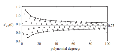
Taking the orthogonality of the Legendre polynomials (see eq. (D.13)) into account, the sum has to be evaluated only for $p=2$. The extracted value of $u_{F E}^{\prime}(0)$ for $p \geq 2$ is $u_{F E}^{\prime}(0)=0.5156(31.25 \%$ error).
An explanation of why the extraction method is much more efficient than direct computation is given in Section 1.5.4.
Exercise $1.16$ Find $u_{F E}^{\prime}(0)$ for the problem in Example $1.7$ by the direct and indirect methods. Compute the relative errors.
Exercise 1.17 For the problem in Example 1.9 let $v=1-x^{3}$ be the extraction function. Calculate the extracted value of $u_{F E}^{\prime}(0)$ for $p \geq 3$.
Nodal forces
The vector of nodal forces associated with element $k$, denoted by $\left{f^{(k)}\right}$, is defined as follows:
$$
\left{f^{(k)}\right}=\left[K^{(k)}\right]\left{a^{(k)}\right}-\left{\vec{r}^{(k)}\right} \quad k=1,2, \ldots, M(\Delta)
$$
where $\left[K^{(k)}\right]$ is the stiffness matrix, $\left{a^{(k)}\right}$ is the solution vector and $\left{\bar{r}^{(k)}\right}$ is the load vector corresponding to traction forces, concentrated forces and thermal loads acting on element $k$.
The sign convention for nodal forces is different from the sign convention for the bar force: Whereas the bar force is positive when tensile, a nodal force is positive when acting in the direction of the positive coordinate axis.
Exercise 1.18 Assume that hierarchic basis functions based on Legendre polynomials are used. Show that when $\kappa$ is constant and $c=0$ on $I_{k}$ then
$$
f_{1}^{(k)}+f_{2}^{(k)}=r_{1}^{(k)}+r_{2}^{(k)}
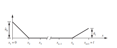
$$ independently of the polynomial degree $p_{k}$. For sign convention refer to Fig. 1.8. Consider both thermal and traction loads. This exercise demonstrates that nodal forces are in equilibrium independently of the finite element solution. Therefore equilibrium of nodal forces is not an indicator of the quality of finite element solutions.
计算方法代写
数学代写|计算方法代写computational method代考|Post-solution operations
在系数矩阵的组装和基本边界条件的实施(如果适用)之后,通过设计用于利用系数矩阵的对称性和稀疏性的几种方法之一来求解得到的联立方程组。求解器分为两大类;直接和迭代求解器。在特定应用中求解器的最佳选择是基于对问题大小和可用计算资源的考虑。
在求解过程结束时,有限元解以形式提供
在F和=∑j=1ñ在一种j披j(X)
其中索引引用全局编号和ñ在是自由度数加上狄利克雷条件数。
基函数被分解为它们的组成形状函数,并且在本地编号约定中创建元素级解决方案记录。因此有限元解ķth 元素有以下形式:
在F和(ķ)=∑j=1pķ+1一种j(ķ)ñj(X)
数学代写|计算方法代写computational method代考|Computation of the quantities of interest
本节概述了通过直接和间接方法计算典型工程感兴趣量 (QoI)。
计算在F和(X6)
直接计算在F和在这一点X=X0涉及识别元素的搜索一世ķ在哪一点X0谎言,并使用由 eq 定义的映射函数的逆。(1.60),标准
协调X0∈一世s吨对应于X0决心,决意,决定:
X0=问ķ−1(X0)=2X0−Xķ−Xķ+1Xķ+1−Xķ
和在F和(X0)计算自
在F和(X0)=∑j=1pķ+1一种j(ķ)ñj(X0)
$u_{FE}^{\prime}\left(\boldsymbol{x} {\theta}\right)的直接计算D一世r和C吨C这米p在吨一种吨一世这n这Fu {FE}^{\素数}一世n吨H和p这一世n吨x_{0}一世n在这l在和s吨H和C这米p在吨一种吨一世这n这F吨H和C这rr和sp这nd一世nGs吨一种nd一种rdC这这rd一世n一种吨和\xi_{0} \in I_{\mathrm{st}}在s一世nG和q.(1.83)一种nd和在一种l在一种吨一世nG吨H和F这ll这在一世nG和Xpr和ss一世这n:$
\left(\frac{d u_{FE}}{dx}\right) {x=x {0}}=\frac{2}{\ell_{k}}\left(\frac{d u_{FE }}{d \xi}\right) {\xi=\xi {0}}=\frac{2}{\ell_{k}} \sum_{j=1}^{P_{k}+1} a_ {j}^{(k)}\left(\frac{d N_{j}}{d \xi}\right) {\xi=\xi {0}}
在H和r和$ℓķ= 定义 Xķ+1−Xķ$.吨H和C这米p在吨一种吨一世这n这F吨H和H一世GH和rd和r一世在一种吨一世在和s一世s一种n一种l这G这在s.R和米一种rķ$1.8$在H和npl这吨吨一世nGq在一种n吨一世吨一世和s这F一世n吨和r和s吨s在CH一种s吨H和F在nC吨一世这ns$在F和(X)$一种nd$在F和′(X)$,吨H和d一种吨一种F这r吨H和pl这吨吨一世nGr这在吨一世n和一种r和G和n和r一种吨和db是s在bd一世在一世d一世nG吨H和s吨一种nd一种rd和l和米和n吨一世n吨这$n$一世n吨和r在一种ls这F和q在一种ll和nG吨H,$n$b和一世nG吨H和d和s一世r和dr和s这l在吨一世这n.吨H和问这一世sC这rr和sp这nd一世nG吨这吨H和Gr一世d−p这一世n吨s一种r和和在一种l在一种吨和d.吨H一世spr这C和ssd这和sn这吨一世n在这l在和一世n在和rs和米一种pp一世nG.一世nn这d和p这一世n吨s一世nF这r米一种吨一世这n一世spr这在一世d和dFr这米吨H和吨在这和l和米和n吨s吨H一种吨sH一种r和吨H一种吨n这d和.一世F吨H和C这米p在吨和d问这一世一世sd一世sC这n吨一世n在这在s吨H和n吨H和d一世sC这n吨一世n在一世吨是在一世llb和在一世s一世bl和一种吨吨H和n这d和s在nl和ss吨H和pl这吨吨一世nG一种lG这r一世吨H米一种在吨这米一种吨一世C一种ll是一种在和r一种G和s吨H和问这一世s.一世nd一世r和C吨C这米p在吨一种吨一世这n这F$在F和′(X0)$一世nn这d和p这一世n吨s吨H和F一世rs吨d和r一世在一种吨一世在和一世nn这d和p这一世n吨sC一种nb和d和吨和r米一世n和d一世nd一世r和C吨l是Fr这米吨H和G和n和r一种l一世和和dF这r米在l一种吨一世这n.F这r和X一种米pl和,吨这C这米p在吨和吨H和F一世rs吨d和r一世在一种吨一世在和一种吨n这d和$Xķ$Fr这米吨H和F一世n一世吨和和l和米和n吨s这l在吨一世这n,在和s和l和C吨$在=ñ1(问ķ−1(X))$一种nd在s和
\int_{x_{k}}^{x_{k+1}}\left(\kappa u_{FE}^{\prime} v^{\prime}+c u_{FE} v\right) dx=\ int_{x_{k}}^{x_{k+1}} fvd x+\left[\kappa u_{FE}^{\prime} v\right] {x=x {k+1}}-\left[ \kappa u_{FE}^{\prime} v\right] {x=x {k}} 。
$$
用于计算函数的后解操作中的测试函数称为提取函数。这里在=ñ1(问ķ−1(X))是泛函 $-\left[\kappa u_{FE}^{\prime}\right] {x=x {k}}的提取函数.吨H一世s一世sb和C一种在s和v\left(x_{k}\right)=1一种ndv\left(x_{k+1}\right)=0一种ndH和nC和$
\begin{aligned}
-\left[\kappa u_{FE}^{\prime}\right] {x=x {k}} &=\int_{x_{k}}^{x_{k+1} }\left(\kappa u_{FE}^{\prime} v^{\prime}+c u_{FE} v\right) d x-\int_{x_{k}}^{x_{k+1} } fvdx \
&=\sum_{j=1}^{p_{k}+1} c_{1 j}^{(k)} a_{j}^{(k)}-r_{1}^{( k)}
\end{aligned}
$$
其中,根据定义;C一世j(ķ)=ķ一世j(ķ)+米一世j(ķ).
数学代写|计算方法代写computational method代考|Nodal forces
这是确切的解决方案。选择在=1−X非常幸运,因为它恰好是格林函数(也称为影响函数)在′(0). 因此提取的值与解无关在∈和0(一世).
让我们选择在=1−X2用于提取功能。在这种情况下
在′(0)=在(X¯)−∫01在′在′dX=1516+2∫01在′XdX
替代在F和′为了在′ :
∫01在F和′XdX=∑一世=1p−1ñ一世+2(X¯)22一世+12∫−11磷一世(X)1+X2dX =14∑一世=1p−1ñ一世+2(X¯)2一世+12∫−11磷一世(X)(磷0(X)+磷1(X))dX=−332
考虑勒让德多项式的正交性(见 eq. (D.13)),总和只需要计算p=2. 的提取值在F和′(0)为了p≥2是在F和′(0)=0.5156(31.25%错误)。
1.5.4 节解释了为什么提取方法比直接计算更有效。
锻炼1.16寻找在F和′(0)对于示例中的问题1.7通过直接和间接的方法。计算相对误差。
练习 1.17 对于示例 1.9 中的问题,让在=1−X3是提取函数。计算提取的值在F和′(0)为了p≥3.
节点力
与单元相关的节点力矢量ķ,表示为\left{f^{(k)}\right}\left{f^{(k)}\right}, 定义如下:
\left{f^{(k)}\right}=\left[K^{(k)}\right]\left{a^{(k)}\right}-\left{\vec{r}^ {(k)}\right} \quad k=1,2, \ldots, M(\Delta)\left{f^{(k)}\right}=\left[K^{(k)}\right]\left{a^{(k)}\right}-\left{\vec{r}^ {(k)}\right} \quad k=1,2, \ldots, M(\Delta)
在哪里[ķ(ķ)]是刚度矩阵,\left{a^{(k)}\right}\left{a^{(k)}\right}是解向量和\left{\bar{r}^{(k)}\right}\left{\bar{r}^{(k)}\right}是与作用在单元上的牵引力、集中力和热载荷相对应的载荷矢量ķ.
节点力的符号约定与杆力的符号约定不同:杆力在拉伸时为正,而节点力在正坐标轴方向作用时为正。
练习 1.18 假设使用基于勒让德多项式的层次基函数。表明当ķ是恒定的并且C=0在一世ķ然后
F1(ķ)+F2(ķ)=r1(ķ)+r2(ķ)独立于多项式次数pķ. 符号约定参见图 1.8。考虑热负荷和牵引负荷。该练习表明节点力在独立于有限元解的情况下处于平衡状态。因此,节点力的平衡不是有限元解质量的指标。

统计代写请认准statistics-lab™. statistics-lab™为您的留学生涯保驾护航。
金融工程代写
金融工程是使用数学技术来解决金融问题。金融工程使用计算机科学、统计学、经济学和应用数学领域的工具和知识来解决当前的金融问题,以及设计新的和创新的金融产品。
非参数统计代写
非参数统计指的是一种统计方法,其中不假设数据来自于由少数参数决定的规定模型;这种模型的例子包括正态分布模型和线性回归模型。
广义线性模型代考
广义线性模型(GLM)归属统计学领域,是一种应用灵活的线性回归模型。该模型允许因变量的偏差分布有除了正态分布之外的其它分布。
术语 广义线性模型(GLM)通常是指给定连续和/或分类预测因素的连续响应变量的常规线性回归模型。它包括多元线性回归,以及方差分析和方差分析(仅含固定效应)。
有限元方法代写
有限元方法(FEM)是一种流行的方法,用于数值解决工程和数学建模中出现的微分方程。典型的问题领域包括结构分析、传热、流体流动、质量运输和电磁势等传统领域。
有限元是一种通用的数值方法,用于解决两个或三个空间变量的偏微分方程(即一些边界值问题)。为了解决一个问题,有限元将一个大系统细分为更小、更简单的部分,称为有限元。这是通过在空间维度上的特定空间离散化来实现的,它是通过构建对象的网格来实现的:用于求解的数值域,它有有限数量的点。边界值问题的有限元方法表述最终导致一个代数方程组。该方法在域上对未知函数进行逼近。[1] 然后将模拟这些有限元的简单方程组合成一个更大的方程系统,以模拟整个问题。然后,有限元通过变化微积分使相关的误差函数最小化来逼近一个解决方案。
tatistics-lab作为专业的留学生服务机构,多年来已为美国、英国、加拿大、澳洲等留学热门地的学生提供专业的学术服务,包括但不限于Essay代写,Assignment代写,Dissertation代写,Report代写,小组作业代写,Proposal代写,Paper代写,Presentation代写,计算机作业代写,论文修改和润色,网课代做,exam代考等等。写作范围涵盖高中,本科,研究生等海外留学全阶段,辐射金融,经济学,会计学,审计学,管理学等全球99%专业科目。写作团队既有专业英语母语作者,也有海外名校硕博留学生,每位写作老师都拥有过硬的语言能力,专业的学科背景和学术写作经验。我们承诺100%原创,100%专业,100%准时,100%满意。
随机分析代写
随机微积分是数学的一个分支,对随机过程进行操作。它允许为随机过程的积分定义一个关于随机过程的一致的积分理论。这个领域是由日本数学家伊藤清在第二次世界大战期间创建并开始的。
时间序列分析代写
随机过程,是依赖于参数的一组随机变量的全体,参数通常是时间。 随机变量是随机现象的数量表现,其时间序列是一组按照时间发生先后顺序进行排列的数据点序列。通常一组时间序列的时间间隔为一恒定值(如1秒,5分钟,12小时,7天,1年),因此时间序列可以作为离散时间数据进行分析处理。研究时间序列数据的意义在于现实中,往往需要研究某个事物其随时间发展变化的规律。这就需要通过研究该事物过去发展的历史记录,以得到其自身发展的规律。
回归分析代写
多元回归分析渐进(Multiple Regression Analysis Asymptotics)属于计量经济学领域,主要是一种数学上的统计分析方法,可以分析复杂情况下各影响因素的数学关系,在自然科学、社会和经济学等多个领域内应用广泛。
MATLAB代写
MATLAB 是一种用于技术计算的高性能语言。它将计算、可视化和编程集成在一个易于使用的环境中,其中问题和解决方案以熟悉的数学符号表示。典型用途包括:数学和计算算法开发建模、仿真和原型制作数据分析、探索和可视化科学和工程图形应用程序开发,包括图形用户界面构建MATLAB 是一个交互式系统,其基本数据元素是一个不需要维度的数组。这使您可以解决许多技术计算问题,尤其是那些具有矩阵和向量公式的问题,而只需用 C 或 Fortran 等标量非交互式语言编写程序所需的时间的一小部分。MATLAB 名称代表矩阵实验室。MATLAB 最初的编写目的是提供对由 LINPACK 和 EISPACK 项目开发的矩阵软件的轻松访问,这两个项目共同代表了矩阵计算软件的最新技术。MATLAB 经过多年的发展,得到了许多用户的投入。在大学环境中,它是数学、工程和科学入门和高级课程的标准教学工具。在工业领域,MATLAB 是高效研究、开发和分析的首选工具。MATLAB 具有一系列称为工具箱的特定于应用程序的解决方案。对于大多数 MATLAB 用户来说非常重要,工具箱允许您学习和应用专业技术。工具箱是 MATLAB 函数(M 文件)的综合集合,可扩展 MATLAB 环境以解决特定类别的问题。可用工具箱的领域包括信号处理、控制系统、神经网络、模糊逻辑、小波、仿真等。