计算机代写|深度学习代写deep learning代考|T81-558
如果你也在 怎样代写深度学习Deep Learning 这个学科遇到相关的难题,请随时右上角联系我们的24/7代写客服。深度学习Deep Learning(是机器学习的一种,也是人工智能的一种方法。通过用简单的世界来构建复杂的世界表示,深度学习技术在计算机视觉、语音识别、自然语言处理、临床应用和其他领域取得了最先进的成果——有望(也有可能)改变社会。
深度学习Deep Learning架构,如深度神经网络、深度信念网络、深度强化学习、递归神经网络、卷积神经网络和变形金刚,已被应用于包括计算机视觉、语音识别、自然语言处理、机器翻译、生物信息学、药物设计、医学图像分析、气候科学、材料检测和棋盘游戏程序等领域,它们产生的结果与人类专家的表现相当,在某些情况下甚至超过了人类专家。
statistics-lab™ 为您的留学生涯保驾护航 在代写深度学习deep learning方面已经树立了自己的口碑, 保证靠谱, 高质且原创的统计Statistics代写服务。我们的专家在代写深度学习deep learning代写方面经验极为丰富,各种代写深度学习deep learning相关的作业也就用不着说。
计算机代写|深度学习代写deep learning代考|Criteria of Adequacy
To summarize, a satisfactory explanation for cognitive change consists of at least the following components:
- A description of the explanatory target itself. The latter can be a unique learning event, a particular change that happened for a person at some point in time and place, a type of change (belief revision) or a recurring pattern of change (the learning curve).
- A background theory of the relevant aspect or aspects of the cognitive architecture. It will include a specification of the types of mental representations assumed; the repertoire of basic cognitive processes that create, manipulate and utilize these representations; and the mechanism that passes control among those processes. This background theory serves as a processing context within which the postulated change mechanisms are assumed to operate.
- A repertoire of learning mechanisms. The change produced by a learning mechanism is typically small in scope compared to the explanatory target. The micro-theories proposed in this book distinguish mechanisms for monotonic learning from mechanisms for non-monotonic learning.
- A specification of the triggering conditions under which each learning mechanism tends to occur.
- An articulation of the mechanisms and the triggering conditions vis-à-vis the explanatory target. An explanation is a demonstration that (a) the relevant triggering conditions held in the situation in which the target change is supposed to have happened, and (b) the specified learning mechanisms, if triggered under those conditions, would in fact produce the observed change. If the explanatory target is a pattern of change, then the articulation needs to show why that type of change tends to recur.
- An explanation is the more satisfactory if it comes with an argument to the effect that the postulated change mechanisms scale up, that is, produce observed or plausible outcomes over long periods of time and across system levels.
- Last, but not least, an explanation is more satisfactory if it comes with a demonstration that the postulated learning mechanisms can support successful practice.
In the terminology of the philosophy of science, these seven points are criteria of adequacy. Their satisfaction does not guarantee the truth of a theory. They constitute a test that a purported explanation has to pass in order to be a viable candidate. Bluntly put: If a theory or hypothesis lacks these features, it is not worth considering.
计算机代写|深度学习代写deep learning代考|THE PATH AHEAD
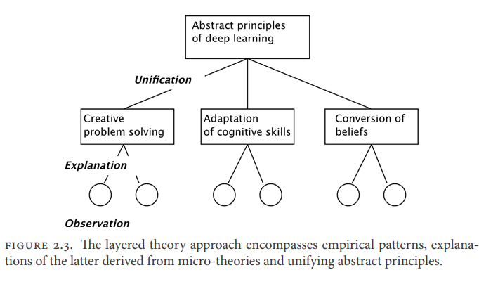
The research strategy behind the investigations reported in this book is to study specific types of non-monotonic change and propose micro-theories to explain them. Once the micro-theories have been clearly formulated, they can be mined for deeper principles, if any. In this approach, theory construction does not proceed in an inductive, bottom-up or top-down fashion. The choice of phenomena to be studied is guided by the prior decision to focus on non-monotonic change, itself a theoretical concept. On the other hand, theory construction does not proceed by pushing a single concept or principle into every corner and crevasse of the cognitive landscape. Instead, the principles of each micro-theory are designed to provide understanding of the case that inspires them without regard for their applicability elsewhere. The deeper theory, if any, is to emerge from the conceptual analysis of the micro-theories. In this layered approach, the degree of unification to be sought is itself an outcome of the investigation rather than something given at the outset. Figure 2.3 shows the overall structure of the enterprise.
Following this strategy, Parts II-IV investigate three cases of nonmonotonic change: the creation of novelty, adaptation to an unfamiliar or changing task environment, and conversion from one belief system to another.
The factor that unites these three types of cognitive change is that they require the learner to overcome some part of his prior knowledge, the distinctive feature of non-monotonic learning. They are separated by the key phenomena, the learning scenarios and experimental paradigms in which we can observe those phenomena and the intellectual traditions within which past explanations for those phenomena have been embedded.
Parts II and III consist of three chapters each. The first chapter in each part frames the theoretical problem to be solved, anchoring it in everyday experience as well as in prior research. The latter includes any work that addresses the relevant problem, regardless of age or disciplinary label. In the second chapter, I state a micro-theory for the relevant explanatory target. In the third chapter, I develop the broader implications of the micro-theory, especially in regard to its interactions with other processes, the accumulation of changes over time and the projection of its effects across system levels. Part IV follows the same schema, except that the third chapter is absent.
深度学习代写
计算机代写|深度学习代写deep learning代考|Criteria of Adequacy
总而言之,对认知变化的一个令人满意的解释至少包括以下几个部分:
对解释对象本身的描述。后者可以是一个独特的学习事件,一个人在某个时间和地点发生的特定变化,一种变化(信念修正)或反复出现的变化模式(学习曲线)。
认知体系的相关方面或方面的背景理论。它将包括对假定的心理表征类型的说明;创造、操纵和利用这些表征的基本认知过程;以及在这些过程之间传递控制的机制。这个背景理论作为一个处理环境,在这个环境中,假设的变化机制被假设运作。
一整套学习机制。与解释目标相比,学习机制产生的变化通常是很小的。本书提出的微观理论区分了单调学习机制和非单调学习机制。
每种学习机制发生的触发条件的说明。
对-à-vis解释目标的机制和触发条件的阐述。解释是证明(a)在目标变化发生的情境中存在相关触发条件,以及(b)在这些条件下触发的特定学习机制实际上会产生观察到的变化。如果解释性目标是一种变化模式,那么表述需要显示为什么这种类型的变化倾向于重复出现。
如果一个解释带有这样的论点,即假设的变化机制按比例扩大,也就是说,在很长一段时间内和跨系统级别产生可观察到的或似是而非的结果,那么这个解释就更令人满意。
最后,但并非最不重要的是,如果一个解释能够证明假设的学习机制能够支持成功的实践,那么这个解释就会更令人满意。
用科学哲学的术语来说,这七点就是充分性的标准。他们的满意并不能保证理论的真实性。它们构成了一种测试,一个声称的解释必须通过这个测试才能成为一个可行的候选者。坦率地说:如果一个理论或假设缺乏这些特征,它就不值得考虑。
计算机代写|深度学习代写deep learning代考|THE PATH AHEAD
本书中报告的调查背后的研究策略是研究特定类型的非单调变化,并提出微观理论来解释它们。一旦微观理论被清晰地表述出来,它们就可以被挖掘出更深层次的原理,如果有的话。在这种方法中,理论构建不是以归纳、自下而上或自上而下的方式进行的。要研究的现象的选择是由先前决定关注非单调变化指导的,非单调变化本身就是一个理论概念。另一方面,理论建设不是将单一的概念或原则推到认知景观的每一个角落和裂缝中。相反,每一种微观理论的原则都旨在提供对激发它们的案例的理解,而不考虑它们在其他地方的适用性。更深层次的理论,如果有的话,是从微观理论的概念分析中产生的。在这种分层的方法中,要寻求的统一程度本身就是调查的结果,而不是一开始就给出的东西。企业整体结构如图2.3所示。
根据这一策略,第二至第四部分研究了三种非单调变化的情况:创造新颖性,适应不熟悉或不断变化的任务环境,以及从一种信仰体系转变为另一种信仰体系。
将这三种类型的认知变化联系在一起的因素是,它们都要求学习者克服其先前知识的某些部分,这是非单调学习的显著特征。它们被关键现象、学习场景和实验范式分开,我们可以在这些现象中观察到这些现象,以及过去对这些现象的解释所包含的知识传统。
第二部分和第三部分各由三章组成。每个部分的第一章都是要解决的理论问题,将其固定在日常经验和先前的研究中。后者包括任何解决相关问题的工作,无论年龄或学科标签如何。在第二章中,我为相关的解释对象阐述了一个微观理论。在第三章中,我发展了微观理论的更广泛的含义,特别是关于它与其他过程的相互作用,随时间变化的积累以及它在系统水平上的影响的预测。第四部分遵循同样的模式,只是没有第三章。

统计代写请认准statistics-lab™. statistics-lab™为您的留学生涯保驾护航。
金融工程代写
金融工程是使用数学技术来解决金融问题。金融工程使用计算机科学、统计学、经济学和应用数学领域的工具和知识来解决当前的金融问题,以及设计新的和创新的金融产品。
非参数统计代写
非参数统计指的是一种统计方法,其中不假设数据来自于由少数参数决定的规定模型;这种模型的例子包括正态分布模型和线性回归模型。
广义线性模型代考
广义线性模型(GLM)归属统计学领域,是一种应用灵活的线性回归模型。该模型允许因变量的偏差分布有除了正态分布之外的其它分布。
术语 广义线性模型(GLM)通常是指给定连续和/或分类预测因素的连续响应变量的常规线性回归模型。它包括多元线性回归,以及方差分析和方差分析(仅含固定效应)。
有限元方法代写
有限元方法(FEM)是一种流行的方法,用于数值解决工程和数学建模中出现的微分方程。典型的问题领域包括结构分析、传热、流体流动、质量运输和电磁势等传统领域。
有限元是一种通用的数值方法,用于解决两个或三个空间变量的偏微分方程(即一些边界值问题)。为了解决一个问题,有限元将一个大系统细分为更小、更简单的部分,称为有限元。这是通过在空间维度上的特定空间离散化来实现的,它是通过构建对象的网格来实现的:用于求解的数值域,它有有限数量的点。边界值问题的有限元方法表述最终导致一个代数方程组。该方法在域上对未知函数进行逼近。[1] 然后将模拟这些有限元的简单方程组合成一个更大的方程系统,以模拟整个问题。然后,有限元通过变化微积分使相关的误差函数最小化来逼近一个解决方案。
tatistics-lab作为专业的留学生服务机构,多年来已为美国、英国、加拿大、澳洲等留学热门地的学生提供专业的学术服务,包括但不限于Essay代写,Assignment代写,Dissertation代写,Report代写,小组作业代写,Proposal代写,Paper代写,Presentation代写,计算机作业代写,论文修改和润色,网课代做,exam代考等等。写作范围涵盖高中,本科,研究生等海外留学全阶段,辐射金融,经济学,会计学,审计学,管理学等全球99%专业科目。写作团队既有专业英语母语作者,也有海外名校硕博留学生,每位写作老师都拥有过硬的语言能力,专业的学科背景和学术写作经验。我们承诺100%原创,100%专业,100%准时,100%满意。
随机分析代写
随机微积分是数学的一个分支,对随机过程进行操作。它允许为随机过程的积分定义一个关于随机过程的一致的积分理论。这个领域是由日本数学家伊藤清在第二次世界大战期间创建并开始的。
时间序列分析代写
随机过程,是依赖于参数的一组随机变量的全体,参数通常是时间。 随机变量是随机现象的数量表现,其时间序列是一组按照时间发生先后顺序进行排列的数据点序列。通常一组时间序列的时间间隔为一恒定值(如1秒,5分钟,12小时,7天,1年),因此时间序列可以作为离散时间数据进行分析处理。研究时间序列数据的意义在于现实中,往往需要研究某个事物其随时间发展变化的规律。这就需要通过研究该事物过去发展的历史记录,以得到其自身发展的规律。
回归分析代写
多元回归分析渐进(Multiple Regression Analysis Asymptotics)属于计量经济学领域,主要是一种数学上的统计分析方法,可以分析复杂情况下各影响因素的数学关系,在自然科学、社会和经济学等多个领域内应用广泛。
MATLAB代写
MATLAB 是一种用于技术计算的高性能语言。它将计算、可视化和编程集成在一个易于使用的环境中,其中问题和解决方案以熟悉的数学符号表示。典型用途包括:数学和计算算法开发建模、仿真和原型制作数据分析、探索和可视化科学和工程图形应用程序开发,包括图形用户界面构建MATLAB 是一个交互式系统,其基本数据元素是一个不需要维度的数组。这使您可以解决许多技术计算问题,尤其是那些具有矩阵和向量公式的问题,而只需用 C 或 Fortran 等标量非交互式语言编写程序所需的时间的一小部分。MATLAB 名称代表矩阵实验室。MATLAB 最初的编写目的是提供对由 LINPACK 和 EISPACK 项目开发的矩阵软件的轻松访问,这两个项目共同代表了矩阵计算软件的最新技术。MATLAB 经过多年的发展,得到了许多用户的投入。在大学环境中,它是数学、工程和科学入门和高级课程的标准教学工具。在工业领域,MATLAB 是高效研究、开发和分析的首选工具。MATLAB 具有一系列称为工具箱的特定于应用程序的解决方案。对于大多数 MATLAB 用户来说非常重要,工具箱允许您学习和应用专业技术。工具箱是 MATLAB 函数(M 文件)的综合集合,可扩展 MATLAB 环境以解决特定类别的问题。可用工具箱的领域包括信号处理、控制系统、神经网络、模糊逻辑、小波、仿真等。