理论计算机代写

分类：理论计算机代写

数学代写|理论计算机代写theoretical computer science代考|Our Proposed Algorithm

Posted on 2022年5月18日2022年5月18日 by statistics-lab

如果你也在怎样代写理论计算机theoretical computer science这个学科遇到相关的难题，请随时右上角联系我们的24/7代写客服。

理论计算机科学在精神上是数学的和抽象的，但它的动机来自于实际和日常的计算。它的目的是理解计算的本质，并作为这种理解的结果，提供更有效的方法论。

statistics-lab™ 为您的留学生涯保驾护航在代写理论计算机theoretical computer science方面已经树立了自己的口碑, 保证靠谱, 高质且原创的统计Statistics代写服务。我们的专家在代写理论计算机theoretical computer science代写方面经验极为丰富，各种代写理论计算机theoretical computer science相关的作业也就用不着说。

我们提供的理论计算机theoretical computer science及其相关学科的代写，服务范围广, 其中包括但不限于:

Statistical Inference 统计推断
Statistical Computing 统计计算
Advanced Probability Theory 高等概率论
Advanced Mathematical Statistics 高等数理统计学
(Generalized) Linear Models 广义线性模型
Statistical Machine Learning 统计机器学习
Longitudinal Data Analysis 纵向数据分析
Foundations of Data Science 数据科学基础

数学代写|理论计算机代写theoretical computer science代考|Our Proposed Algorithm

The proposed framework and algorithm is described in this section. The classifier works better with more labeled data, unlabeled data is much more than labeled data in semi supervised algorithms. If unlabeled data is labeled correctly and added to the labeled set, performance of the classifier improves.

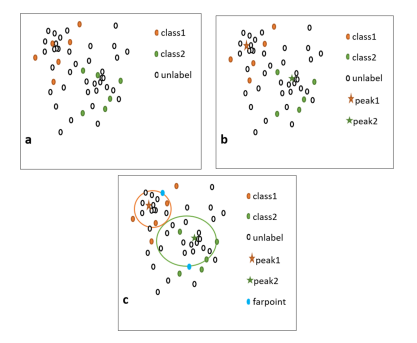
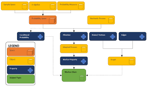
Our proposed algorithm is a semi-supervised self-training algorithm. Figure 4 shows the steps of the proposed framework. In the first step, we find $\delta$ and $\rho$ for all training data set (labeled and unlabeled) and then the high density peaks are found in the labeled data set. The number of peaks is the number of classes. Then, for each peak we find corresponding far point. Step 2 consists of two parts. One section is about selecting a set of unlabeled data which is the candidate for labeling. The distance of all unlabeled data are calculated from decision boundary. Next unlabeled data are selected for labeling that are closer to the decision boundary. Threshold (distance of decision boundary) is considered the mean distance of all unlabeled data from decision boundary.

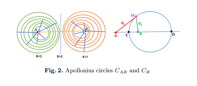
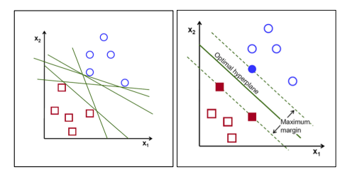
Another part of this step is how to label unlabeled data. Our proposed method predicts the label of unlabeled data by high density peak and Apollonius circle concepts. The label of peak $k_{i}$ is assigned to the unlabeled data that are inside the Apollonius circle corresponding $p e a k_{i}$ and in parallel the same unlabeled subset is given to SVM to label them. The agreement based on the classifier predictions and Apollonius circle is used to select a newly-labeled set The labeled set is updated and is used to retrain the classifier. The process is repeated until it reaches the stopping condition. Figure 4 represents the overview of proposed algorithm.

数学代写|理论计算机代写theoretical computer science代考|Experimental Setup

In this section, we perform several experiments to compare the classification performance of our proposed algorithm to the state-of-the-art semi-supervised methods using several different datasets. We also setup several experiments to show, the impact of selecting data close the decision boundary for improving the classification performance.

In the experiment, some UCI datasets are used. Table 1 summarizes the specification of 8 benchmark datasets from the UCI data repository which are used in our experiments.For each dataset, $30 \%$ of data are kept as test set randomly and the rest are used for training set. The training set is divided into two sets of labeled data and unlabeled data. Classes are selected at a proportions equal to the original dataset for all sets. Initially, we have assigned $5 \%$ to the labeled data and $95 \%$ to the unlabeled data. We have repeated each experiment ten times with different subsets of training and testing data. We report the mean accuracy rate (MAR) of 10 times repeating the experiments.

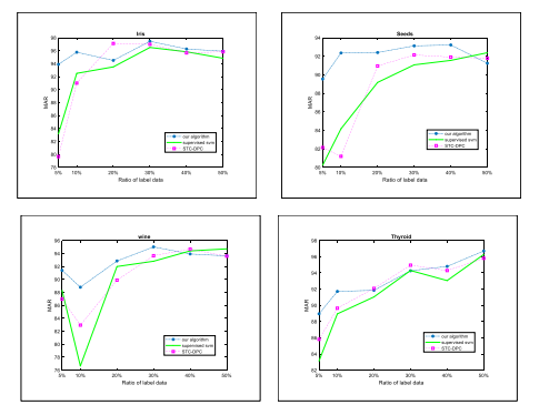
Table 2 shows the comparison of our algorithm with some other algorithms when labeled data is $10 \%$. The second and third columns in this table give respectively the performance of the supervised SVM and self-training SVM. The fourth col$u m n$ is the performance of state-of-the-art algorithm that is called STC-DPC algorithm [7]. The last column is the performance of our algorithm. Base learner for all of algorithms is SVM. Cut of distance parameter (dc) for our algorithm and STC-DPC is $0.05$. From Table 2 , we observe that Our algorithm works well for datasets that have a separate data density such as Iris, Seeds, Wine. Our proposed algorithm doesn’t work very well if dataset is very mixed, such as banknote Fig. 5 and Fig. 6. We also investigate the behavior of the algorithms based on increasing ratio of labeled data. Fig. 7 is a comparison of the three algorithms with the increase ratio of label data from $5 \%$ to $50 \%$.

数学代写|理论计算机代写theoretical computer science代考|Impact of Selecting Data Close the Decision Boundary

In most datasets, labeling all unlabeled data can not improve the performance but also reduces the accuracy. In addition to decreasing accuracy, runtime is also increased. Although the unlabeled data that are far from the decision boundary are more reliable, they are not informative. They play little role in improving decision boundary. That’s why we haven’t added all the unlabeled data to the

training set, rather, we add those that are closer to the decision boundary than a certain value.

We show the results on a number of datasets in Table 3 . The second column is the accuracy of our algorithm when we have added all the unlabeled data and the third column is the accuracy of our algorithm when we add only the data point closes to the decision boundary. As can be seen from Table 3 , the accuracy of the algorithm increases when we only add unlabeled data closer to the decision boundary instead of all the points.

In this paper, we proposed a semi-supervised self-training method based on Apollonius, named SSApolo. First candidate data are selected from among the unlabeled data to be labeled in the self training process, then, using the density peak clustering, the peak points are found and by making an Apollonius circle of each peak points, their neighbors are found and labeled. Support vector machine is used for classification. A series of experiments was performed on some datasets and the performance of the proposed algorithm was evaluated. According to the experimental results, we conclude that our algorithm performs better than STCDPC algorithm and supervised SVM and self-training SVM, especially when classes of dataset are not very mixed. In addition, the impact of selecting data are close to decision boundary was investigated. We find that selecting data are close to decision boundary can improves the performance.

数学代写|理论计算机代写theoretical computer science代考|Our Proposed Algorithm

本节描述了所提出的框架和算法。分类器对更多标记数据的效果更好，未标记数据比半监督算法中的标记数据要多得多。如果未标记的数据被正确标记并添加到标记集，则分类器的性能会提高。

我们提出的算法是一种半监督自训练算法。图 4 显示了建议框架的步骤。第一步，我们发现d和ρ对于所有训练数据集（标记和未标记），然后在标记数据集中找到高密度峰值。峰值的数量是类的数量。然后，对于每个峰值，我们找到对应的远点。步骤 2 由两部分组成。一个部分是关于选择一组未标记的数据作为标记的候选者。所有未标记数据的距离都是从决策边界计算的。选择下一个未标记的数据进行更接近决策边界的标记。阈值（决策边界的距离）被认为是所有未标记数据与决策边界的平均距离。

此步骤的另一部分是如何标记未标记的数据。我们提出的方法通过高密度峰值和阿波罗环概念来预测未标记数据的标签。巅峰的标签ķ一世分配给对应的阿波罗尼星圈内的未标记数据p和一种ķ一世并且并行地将相同的未标记子集提供给 SVM 以标记它们。基于分类器预测和 Apollonius 圆的协议用于选择新标记集。标记集被更新并用于重新训练分类器。重复该过程，直到达到停止条件。图 4 代表了所提出算法的概述。

数学代写|理论计算机代写theoretical computer science代考|Experimental Setup

在本节中，我们进行了几个实验，以将我们提出的算法的分类性能与使用几个不同数据集的最先进的半监督方法进行比较。我们还设置了几个实验来展示选择接近决策边界的数据对提高分类性能的影响。

在实验中，使用了一些 UCI 数据集。表 1 总结了我们实验中使用的 UCI 数据存储库中 8 个基准数据集的规范。对于每个数据集，30%数据随机保存为测试集，其余用于训练集。训练集分为标记数据和未标记数据两组。以与所有集合的原始数据集相同的比例选择类。最初，我们分配了5%标记数据和95%到未标记的数据。我们用不同的训练和测试数据子集重复了每个实验十次。我们报告了重复实验 10 次的平均准确率 (MAR)。

表 2 显示了我们的算法与其他一些算法在标记数据时的比较10%. 该表中的第二列和第三列分别给出了监督 SVM 和自训练 SVM 的性能。第四栏在米n是最先进算法的性能，称为 STC-DPC 算法 [7]。最后一列是我们算法的性能。所有算法的基础学习器都是 SVM。我们的算法和 STC-DPC 的距离参数 (dc) 为0.05. 从表 2 中，我们观察到我们的算法适用于具有单独数据密度的数据集，例如 Iris、Seeds、Wine。如果数据集非常混合，例如钞票图 5 和图 6，我们提出的算法就不能很好地工作。我们还研究了基于标记数据比例增加的算法的行为。图 7 是三种算法与标签数据增加率的比较5%到50%.

数学代写|理论计算机代写theoretical computer science代考|Impact of Selecting Data Close the Decision Boundary

在大多数数据集中，标记所有未标记的数据并不能提高性能，还会降低准确性。除了降低准确性之外，运行时间也增加了。尽管远离决策边界的未标记数据更可靠，但它们没有提供信息。它们在改善决策边界方面几乎没有作用。这就是为什么我们没有将所有未标记的数据添加到

相反，我们添加了那些比某个值更接近决策边界的训练集。

我们在表 3 中展示了多个数据集的结果。第二列是当我们添加了所有未标记的数据时我们算法的准确度，第三列是当我们只添加接近决策边界的数据点时我们的算法的准确度。从表 3 可以看出，当我们只添加更靠近决策边界的未标记数据而不是所有点时，算法的准确性会提高。

在本文中，我们提出了一种基于 Apollonius 的半监督自训练方法，命名为 SSAPolo。在自训练过程中，首先从待标注的未标注数据中选择候选数据，然后利用密度峰值聚类，找到峰值点，并通过对每个峰值点做一个阿波罗圆，找到并标记它们的邻居。支持向量机用于分类。在一些数据集上进行了一系列实验，并评估了所提出算法的性能。根据实验结果，我们得出结论，我们的算法比 STCDPC 算法和监督 SVM 和自训练 SVM 表现更好，尤其是当数据集的类别不是很混合时。此外，研究了选择接近决策边界的数据的影响。

数学代写|理论计算机代写theoretical computer science代考请认准statistics-lab™

统计代写请认准statistics-lab™. statistics-lab™为您的留学生涯保驾护航。

金融工程代写

金融工程是使用数学技术来解决金融问题。金融工程使用计算机科学、统计学、经济学和应用数学领域的工具和知识来解决当前的金融问题，以及设计新的和创新的金融产品。

非参数统计代写

非参数统计指的是一种统计方法，其中不假设数据来自于由少数参数决定的规定模型；这种模型的例子包括正态分布模型和线性回归模型。

广义线性模型代考

广义线性模型（GLM）归属统计学领域，是一种应用灵活的线性回归模型。该模型允许因变量的偏差分布有除了正态分布之外的其它分布。

术语广义线性模型（GLM）通常是指给定连续和/或分类预测因素的连续响应变量的常规线性回归模型。它包括多元线性回归，以及方差分析和方差分析（仅含固定效应）。

有限元方法代写

有限元方法（FEM）是一种流行的方法，用于数值解决工程和数学建模中出现的微分方程。典型的问题领域包括结构分析、传热、流体流动、质量运输和电磁势等传统领域。

有限元是一种通用的数值方法，用于解决两个或三个空间变量的偏微分方程（即一些边界值问题）。为了解决一个问题，有限元将一个大系统细分为更小、更简单的部分，称为有限元。这是通过在空间维度上的特定空间离散化来实现的，它是通过构建对象的网格来实现的：用于求解的数值域，它有有限数量的点。边界值问题的有限元方法表述最终导致一个代数方程组。该方法在域上对未知函数进行逼近。[1] 然后将模拟这些有限元的简单方程组合成一个更大的方程系统，以模拟整个问题。然后，有限元通过变化微积分使相关的误差函数最小化来逼近一个解决方案。

tatistics-lab作为专业的留学生服务机构，多年来已为美国、英国、加拿大、澳洲等留学热门地的学生提供专业的学术服务，包括但不限于Essay代写，Assignment代写，Dissertation代写，Report代写，小组作业代写，Proposal代写，Paper代写，Presentation代写，计算机作业代写，论文修改和润色，网课代做，exam代考等等。写作范围涵盖高中，本科，研究生等海外留学全阶段，辐射金融，经济学，会计学，审计学，管理学等全球99%专业科目。写作团队既有专业英语母语作者，也有海外名校硕博留学生，每位写作老师都拥有过硬的语言能力，专业的学科背景和学术写作经验。我们承诺100%原创，100%专业，100%准时，100%满意。

随机分析代写

随机微积分是数学的一个分支，对随机过程进行操作。它允许为随机过程的积分定义一个关于随机过程的一致的积分理论。这个领域是由日本数学家伊藤清在第二次世界大战期间创建并开始的。

时间序列分析代写

随机过程，是依赖于参数的一组随机变量的全体，参数通常是时间。随机变量是随机现象的数量表现，其时间序列是一组按照时间发生先后顺序进行排列的数据点序列。通常一组时间序列的时间间隔为一恒定值（如1秒，5分钟，12小时，7天，1年），因此时间序列可以作为离散时间数据进行分析处理。研究时间序列数据的意义在于现实中，往往需要研究某个事物其随时间发展变化的规律。这就需要通过研究该事物过去发展的历史记录，以得到其自身发展的规律。

回归分析代写

多元回归分析渐进（Multiple Regression Analysis Asymptotics）属于计量经济学领域，主要是一种数学上的统计分析方法，可以分析复杂情况下各影响因素的数学关系，在自然科学、社会和经济学等多个领域内应用广泛。

MATLAB代写

MATLAB 是一种用于技术计算的高性能语言。它将计算、可视化和编程集成在一个易于使用的环境中，其中问题和解决方案以熟悉的数学符号表示。典型用途包括：数学和计算算法开发建模、仿真和原型制作数据分析、探索和可视化科学和工程图形应用程序开发，包括图形用户界面构建MATLAB 是一个交互式系统，其基本数据元素是一个不需要维度的数组。这使您可以解决许多技术计算问题，尤其是那些具有矩阵和向量公式的问题，而只需用 C 或 Fortran 等标量非交互式语言编写程序所需的时间的一小部分。MATLAB 名称代表矩阵实验室。MATLAB 最初的编写目的是提供对由 LINPACK 和 EISPACK 项目开发的矩阵软件的轻松访问，这两个项目共同代表了矩阵计算软件的最新技术。MATLAB 经过多年的发展，得到了许多用户的投入。在大学环境中，它是数学、工程和科学入门和高级课程的标准教学工具。在工业领域，MATLAB 是高效研究、开发和分析的首选工具。MATLAB 具有一系列称为工具箱的特定于应用程序的解决方案。对于大多数 MATLAB 用户来说非常重要，工具箱允许您学习和应用专业技术。工具箱是 MATLAB 函数（M 文件）的综合集合，可扩展 MATLAB 环境以解决特定类别的问题。可用工具箱的领域包括信号处理、控制系统、神经网络、模糊逻辑、小波、仿真等。

R语言代写	问卷设计与分析代写
PYTHON代写	回归分析与线性模型代写
MATLAB代写	方差分析与试验设计代写
STATA代写	机器学习/统计学习代写
SPSS代写	计量经济学代写
EVIEWS代写	时间序列分析代写
EXCEL代写	深度学习代写
SQL代写	各种数据建模与可视化代写

数学代写|理论计算机代写theoretical computer science代考|Margin-Based Semi-supervised Learning

Posted on 2022年5月18日2022年5月18日 by statistics-lab

如果你也在怎样代写理论计算机theoretical computer science这个学科遇到相关的难题，请随时右上角联系我们的24/7代写客服。

我们提供的理论计算机theoretical computer science及其相关学科的代写，服务范围广, 其中包括但不限于:

Statistical Inference 统计推断
Statistical Computing 统计计算
Advanced Probability Theory 高等概率论
Advanced Mathematical Statistics 高等数理统计学
(Generalized) Linear Models 广义线性模型
Statistical Machine Learning 统计机器学习
Longitudinal Data Analysis 纵向数据分析
Foundations of Data Science 数据科学基础

数学代写|理论计算机代写theoretical computer science代考|Margin-Based Semi-supervised Learning

数学代写|理论计算机代写theoretical computer science代考|Review of Concepts Related to the Density Peaks and the Apollonius Circle

In this section, the concepts of the Apollonius circle are discussed. We propose the neighborhood structure of the Apollonius circle to label the unlabeled data.
Apollonius circle is one of the most famous problems in geometry [18]. The goal is to find accurate neighborhoods. In a set of points, there is no information about the relationship between the points and some databases may not even contain topological information. It is more accurate than the Gabriel graph [25] and neighborhood graph in the neighborhood construction. It evaluates important neighborhood entirely. In this method, the first step is to find high density points and the second step is to build neighborhood groups with the Apollonius circle. The third step is analyzing points outside the radius of the Apollonian circles or points within the region.

数学代写|理论计算机代写theoretical computer science代考|Finding High Density Points

Rodriguez and Laio [20] presented the algorithm to find high density points (DPC). The high density points are found by this method and then stored in an array.

The points are shown by the vector $\mathbf{M}=\left(M_{1 i}, M_{2 i}, \ldots, M_{m i}\right)$ where $m$ is the number of attributes, also $N_{M_{i}}$ shows $k$ nearest neighbors of $M_{i} \cdot d\left(M_{i}, M_{j}\right)$ is the Euclidean distance between $M_{i}$ and $M_{j}$. The percent of the neighborhood is shown by $p$. The number of neighbors is obtained by $r=p \times n$, where $n$ is the number of data points. The local density $\rho_{i}$ is then defined as:
$$
\begin{gathered}
\rho_{i}=\exp \left(-\left(\frac{1}{r} \sum_{M_{j} \in N\left(M_{i}\right)} d\left(M_{i}, M_{J}\right)^{2}\right)\right) \
d\left(M_{i}, M_{j}\right)=\left|M_{i}-M_{j}\right|
\end{gathered}
$$
where $\delta_{i}$ is the minimum distance between $M_{i}$ and any other sample with higher density than $p_{i}$, which is define as below:
$$
\delta_{i}= \begin{cases}\min {\rho{i}<\rho_{j}}\left{d\left(M_{i}, M_{j}\right)\right}, & \text { if } \exists j \quad \rho_{i}<\rho_{j} \ \max {j}\left{d\left(M{i}, M_{j}\right)\right}, & \text { otherwise }\end{cases}
$$
Peaks (high density points) are obtained using the score function. The points that have the highest score are considered as peak point.
$$
\operatorname{score}\left(M_{i}\right)=\delta_{i} \times \rho_{i}
$$
In this article, number of peaks are selected based on the number of classes. Peaks are selected from the labeled set. We assign the label of peaks to the unlabeled data based on neighborhood radius of peaks. Neighboring groups are found by the Apollonius circle.

数学代写|理论计算机代写theoretical computer science代考|Neighborhood Groups with the Apollonius Circle

The Apollonius circle is the geometric location of the points on the Euclidean plane which have a specified ratio of distances to two fixed points $\mathrm{A}$ and $\mathrm{B}$, this ratio is called $K$ [17]. Apollonius circle can be seen in Fig. 2 .
$$
K=d_{1} / d_{2} .
$$
The Apollonius circle based on $A$ and $B$ is defined as:
$$
C_{A B}=\left{\begin{array}{lll}
C_{A} & \text { if } & K<1 \\ C_{B} & \text { if } & K>1 \
C_{\text {inf }} & \text { if } & K=1
\end{array}\right.
$$
After finding the high density points, we sort these points. The peak points are indicated by $P=\left(P_{1}, P_{2}, \ldots, P_{m}\right)$ which are arranged in pairs $\left(P_{t}, P_{t+1}\right), t \in{1,2, \ldots, m-1}$, the data points are denoted by $M=$ $\left{M_{i} \mid i \in{1,2, \ldots, n-m}, M_{i} \notin P\right}$. In the next step, data points far from the peak points are determined by the formula 7 . Finally the distance of the furthest point from the peak points is calculated by the formula 8 .
$$
\begin{gathered}
F d_{P_{t}}=\max \left{d\left(P_{t}, M_{i}\right) \mid M_{i} \in M \text { and } d\left(P_{t}, M_{i}\right)<d\left(P_{t}, P_{t+1}\right)\right. \
\text { and } \left.d\left(P_{t}, M_{i}\right)<\min {l=1, l \in P} d\left(P{l}, M_{i}\right) \text { s.t. } t \neq l\right} \
F P_{t}=\left{M_{i} \mid d\left(P_{t}, M_{i}\right)=F d_{t}\right} .
\end{gathered}
$$
The points between the peak point and the far point are inside the Apollonius circle, circle [18].

The above concepts are used to label the unlabeled samples confidently. In our proposed algorithm, label of the peak points are assigned to the unlabeled example which are inside the Apollonius circle. The steps are shown in Fig. 3 .

理论计算机代写

数学代写|理论计算机代写theoretical computer science代考|Review of Concepts Related to the Density Peaks and the Apollonius Circle

在本节中，将讨论 Apollonius 圆的概念。我们提出了 Apollonius 圆的邻域结构来标记未标记的数据。
阿波罗尼奥斯圆是几何学中最著名的问题之一[18]。目标是找到准确的邻域。在一组点中，没有关于点之间关系的信息，有些数据库甚至可能不包含拓扑信息。它比邻域构造中的 Gabriel 图 [25] 和邻域图更准确。它全面评估重要的邻里。在该方法中，第一步是寻找高密度点，第二步是用阿波罗尼圆建立邻域组。第三步是分析日神圆半径外的点或区域内的点。

数学代写|理论计算机代写theoretical computer science代考|Finding High Density Points

Rodriguez 和 Laio [20] 提出了寻找高密度点 (DPC) 的算法。通过这种方法找到高密度点，然后将其存储在数组中。

点由矢量显示米=(米1一世,米2一世,…,米米一世)在哪里米是属性的数量，也是ñ米一世节目ķ最近的邻居米一世⋅d(米一世,米j)是之间的欧几里得距离米一世和米j. 邻域的百分比由下式表示p. 邻居的数量由下式获得r=p×n，在哪里n是数据点的数量。局部密度ρ一世则定义为：
ρ一世=经验⁡(−(1r∑米j∈ñ(米一世)d(米一世,米Ĵ)2)) d(米一世,米j)=|米一世−米j|
在哪里d一世是之间的最小距离米一世和任何其他密度更高的样品p一世，其定义如下：
\delta_{i}= \begin{cases}\min {\rho{i}<\rho_{j}}\left{d\left(M_{i}, M_{j}\right)\right}, & \text { if } \exists j \quad \rho_{i}<\rho_{j} \ \max {j}\left{d\left(M{i}, M_{j}\right)\right}， & \text { 否则 }\end{cases}\delta_{i}= \begin{cases}\min {\rho{i}<\rho_{j}}\left{d\left(M_{i}, M_{j}\right)\right}, & \text { if } \exists j \quad \rho_{i}<\rho_{j} \ \max {j}\left{d\left(M{i}, M_{j}\right)\right}， & \text { 否则 }\end{cases}
使用评分函数获得峰值（高密度点）。得分最高的点被认为是峰值点。
分数⁡(米一世)=d一世×ρ一世
在本文中，峰值的数量是根据类的数量来选择的。从标记的集合中选择峰。我们根据峰的邻域半径将峰的标签分配给未标记的数据。阿波罗尼乌斯圈发现了相邻的群体。

数学代写|理论计算机代写theoretical computer science代考|Neighborhood Groups with the Apollonius Circle

阿波罗圆是欧几里得平面上的点的几何位置，这些点与两个固定点具有指定的距离比一种和乙，这个比例称为ķ[17]。Apollonius圆可以在图2中看到。
ķ=d1/d2.
基于阿波罗尼乌斯圆一种和乙定义为：
$$
C_{AB}=\left{C一种如果 ķ<1C乙如果 ķ>1 C信息如果 ķ=1\对。
找到高密度点后，我们对这些点进行排序。峰值点由 $P=\left(P_{1}, P_{2}, \ldots, P_{m}\right)$ 表示，它们成对排列 $\left(P_{t}, P_{t +1}\right), t \in{1,2, \ldots, m-1}$，数据点记为$M=$ $\left{M_{i} \mid i \in{1, 2, \ldots, nm}, M_{i} \notin P\right}$。在下一步中，远离峰值点的数据点由公式7确定。最后通过公式8计算最远点到峰值点的距离。找到高密度点后，我们对这些点进行排序。峰值点由 $P=\left(P_{1}, P_{2}, \ldots, P_{m}\right)$ 表示，它们成对排列 $\left(P_{t}, P_{t +1}\right), t \in{1,2, \ldots, m-1}$，数据点记为$M=$ $\left{M_{i} \mid i \in{1, 2, \ldots, nm}, M_{i} \notin P\right}$。在下一步中，远离峰值点的数据点由公式7确定。最后通过公式8计算最远点到峰值点的距离。
\begin{gathered} F d_{P_{t}}=\max \left{d\left(P_{t}, M_{i}\right) \mid M_{i} \in M \text { and } d \left(P_{t}, M_{i}\right)<d\left(P_{t}, P_{t+1}\right)\right。\ \text { 和 } \left.d\left(P_{t}, M_{i}\right)<\min {l=1, l \in P} d\left(P{l}, M_{i }\right) \text { st } t \neq l\right} \F P_{t}=\left{M_{i} \mid d\left(P_{t}, M_{i}\right)=F d_{t}\right} 。\结束{聚集}\begin{gathered} F d_{P_{t}}=\max \left{d\left(P_{t}, M_{i}\right) \mid M_{i} \in M \text { and } d \left(P_{t}, M_{i}\right)<d\left(P_{t}, P_{t+1}\right)\right。\ \text { 和 } \left.d\left(P_{t}, M_{i}\right)<\min {l=1, l \in P} d\left(P{l}, M_{i }\right) \text { st } t \neq l\right} \F P_{t}=\left{M_{i} \mid d\left(P_{t}, M_{i}\right)=F d_{t}\right} 。\结束{聚集}
$$
峰值点和远点之间的点在阿波罗圆内，圆[18]。

上述概念用于自信地标记未标记的样本。在我们提出的算法中，峰值点的标签被分配给阿波罗尼星圆内的未标记示例。步骤如图3所示。

统计代写请认准statistics-lab™. statistics-lab™为您的留学生涯保驾护航。

金融工程代写

非参数统计代写

非参数统计指的是一种统计方法，其中不假设数据来自于由少数参数决定的规定模型；这种模型的例子包括正态分布模型和线性回归模型。

广义线性模型代考

广义线性模型（GLM）归属统计学领域，是一种应用灵活的线性回归模型。该模型允许因变量的偏差分布有除了正态分布之外的其它分布。

有限元方法代写

随机分析代写

时间序列分析代写

回归分析代写

MATLAB代写

R语言代写	问卷设计与分析代写
PYTHON代写	回归分析与线性模型代写
MATLAB代写	方差分析与试验设计代写
STATA代写	机器学习/统计学习代写
SPSS代写	计量经济学代写
EVIEWS代写	时间序列分析代写
EXCEL代写	深度学习代写
SQL代写	各种数据建模与可视化代写

数学代写|理论计算机代写theoretical computer science代考| Hardness of Exact Computation

Posted on 2022年5月18日2022年5月18日 by statistics-lab

如果你也在怎样代写理论计算机theoretical computer science这个学科遇到相关的难题，请随时右上角联系我们的24/7代写客服。

我们提供的理论计算机theoretical computer science及其相关学科的代写，服务范围广, 其中包括但不限于:

Statistical Inference 统计推断
Statistical Computing 统计计算
Advanced Probability Theory 高等概率论
Advanced Mathematical Statistics 高等数理统计学
(Generalized) Linear Models 广义线性模型
Statistical Machine Learning 统计机器学习
Longitudinal Data Analysis 纵向数据分析
Foundations of Data Science 数据科学基础

数学代写|理论计算机代写theoretical computer science代考|Hardness of Exact Computation

In this section we provide several hardness results for the DOUBLE UPPER EC and the UPPER $r$-EC in some graph classes as regular graphs and split graphs.
Theorem 11. Let $G=(V, E)$ be an $(r+1)$-regular graph with $r \geq 2$. Then,
$$
\operatorname{uec}{r}(G)=|E|-\operatorname{eds}(G) . $$ Proof. In order to prove this equation, first we will show that if $S \subseteq E$ is a $r$-tec of $G$, then $\bar{S}=E \backslash S$ is an edge dominating set of $G$. Let $\left(V{1}, V_{2}\right)$ be the associated partition related to $S$. By the Property 1 we know that $V_{2}$ is an independent set. Because our graph is $(r+1)$-regular, it is easy to see that $\forall v \in V_{1}, d_{G_{S}}(v)=r$ and $\forall u \in V_{2}, d_{G_{S}}(u)=r+1$. This observation gives us that the set $\bar{S}$ covers each vertex of $V_{1}$ (they have degree $r$ ) and that all the edges in $E$ are incident to a vertex in $V_{1}$ (because $V_{2}$ is an independent set). So, $\bar{S}$ is an edge dominating set.

Conversely, let $S$ be a solution of EDS. We will show that there exists a $r$-tec of size $|\bar{S}|$. Because EDS is equivalent to Lower EM, we consider the edge set $S$ as a maximal matching. Now, let $V^{\prime}=V \backslash V[S]$. Observe that $V^{\prime}$ is an independent set in $G$ and each vertex $v \in V^{\prime}$ has $d_{G_{S}}(v)=r+1$. The first holds because if there exists an edge $e$ between two vertices of $V^{\prime}$ then $S \cup{e}$ will be a matching with size greater than $S$, which contradicts the maximality of $S$. The second holds because the edges in $S$ are not incident to vertices of $V^{\prime}$ by definition, and thus, all the edges in $\bar{S}$ are incident to at least one vertex in $V[S]$. Finally, because $S$ is a matching we have that all the vertices in $V[S]$ have degree $r$ in $G_{\bar{S}}$ so by the Property $1, \bar{S}$ is a $r$-tec. So the Eq. (6) holds.
Corollary 12. UPPER $r$-EC is $\mathbf{N P}$-hard in $(r+1)$-regular bipartite graphs.
Proof. Using the NP-hardness proof of EDS in $r$-regular bipartite graphs given in $[15]$, the results follows from Theorem $11 .$
Corollary 13. DOUBLE UPPER EC is NP-hard in cubic planar graphs.
Proof. Using the NP-hardness proof of EDS for cubic planar graphs given in [23], the results follows from Theorem $11 .$

Theorem 14. UPPER $(r+1)$-EC is NP-hard in graphs of maximum degree $\Delta+1$ if UPPER $r$-EC is $N P$-hard in graphs of maximum degree $\Delta$, and this holds even for bipartite graphs.

Proof. Let $G=(V, E)$ be a bipartite graph of maximum degree $\Delta$, we construct a new graph $G^{\prime}=\left(V^{\prime}, E^{\prime}\right)$ by starting from $r+1$ copies of $G$. Then for each vertex $v \in V$ we add a new vertex $u_{v}$ in $G^{\prime}$ and connect it to each one of the $r+1$ copies of the vertex $v$.

数学代写|理论计算机代写theoretical computer science代考|Hardness of Approximation

In the following theorems we provide some inapproximability results for the UPPER EC and the DOUBLE UPPER EC.

Theorem 17. It is NP-hard to approximate the solution of UPPER EC to within $\frac{593}{594}$ and $\frac{363}{364}$ in graphs of max degree 4 and 5 respectively.

Proof. In order to prove this we will use a reduction from Min VC. Starting from an $r$-regular graph $G=(V, E)$ we will construct a new graph $G^{\prime}$; first we add a $P_{2}$ to each vertex $v \in V$. Then for each edge $e=v u \in E$ we add a new vertex $v_{e}$ adjacent to $v$ and $u$. In the end we remove all the starting edges $E$. Since Min VC can not be approximated to within a factor $\frac{100}{99}$ (resp. $\frac{53}{52}$ ) in 3-regular (resp. 4-regular) graphs [11], it deduces the expected results.

Theorem 18. It is NP-hard to approximate the solution of DOUBLE UPPER EC to within $\frac{883}{884}$ in graphs of max degree 6 .

Proof. In order to get the inapproximability result, we first make a reduction from MiN VC to UPPER. EC similar to Theorem 17, then we reduce it to DOUBLE UPPER EC using a reduction proposed in Theorem $14 .$

Theorem 19. It is NP-hard to approximate the solution of DOUBLE UPPER. EC to within $\frac{571}{572}$ in graphs of max degree 9 .

Proof. Again, we will make a reduction from VerTex Cover problem. Starting from a 4-regular graph $G=(V, E)$ we construct a new graph by adding a set of new vertices $V_{E}$ which has one vertex $v_{e}$ for each edge $e \in E$, and then adding new edges $v_{\varepsilon} u$ if the edge $e$ was incident to $u$ in the original graph $G$. Let $G^{\prime}=\left(V^{\prime}, E^{\prime}\right)$ be the new graph. It is easy to see that $\left|V^{\prime}\right|=|V|+|E|$ and $\Delta\left(G^{\prime}\right)=2 \Delta(G)=8$. Furthermore, we can show that from any $V C$ of $G$ we can

construct a tec of $G^{\prime}$ of size $|T E C|=|E|+|V|-|V C|$ and conversely, from any tec of $G^{\prime}$ we can construct a $V C$ of $G$ of size $|V C|=|E|+|V|-|T E C|$. In order to prove the first direction we will start from a $V C$ of $G$. Let $S$ be the set of all the edges $v_{c} u$ where $u \in V C . S$ is a partial tec of $G$ because it covers only the vertices in $V C \cup V_{E}$, any vertex of $V_{E}$ has degree one in $G_{S}^{\prime}$ and the vertices of $V C$ are independent in $G_{S}^{\prime}$. It is easy to extend $S$ to a tec of $G^{\prime}$ by adding one edge for every vertex $v \in V \backslash V C$ that is adjacent to a vertex in $V C$ (there exists because $v \in V$ and $V C$ is a vertex cover of $G$ ). The extended $S$ is a tec due to the fact that the vertices that may have greater degree than one are all in $V C$, which is independent in $G_{S}$ and all the vertices are covered. Now we have to observe that this tec contains exactly one edge for each vertex in $V_{E}$ and one for each vertex in $V \backslash V C$ so the size is exactly
$$
|T E C|=|E|+|V|-|V C| .
$$
Conversely, we will start from a tec of $G^{\prime}$ and we will construct a vertex cover of $G$ of the wanted size. First we have to show that for any tec $S$ of $G^{\prime}$, if there exists $v_{e} \in V_{E}$ such that $d_{G_{s}^{\prime}}\left(v_{e}\right)=2$ (it can not be greater because $d_{G^{\prime}}\left(v_{c}\right)=2$ ) then there exists an other tec $S^{\prime}$ of $G^{\prime}$ that has the same size and every vertex $v_{e} \in V_{E}$ has degree $d_{G_{S^{\prime}}}\left(v_{e}\right)=1$. This is easy to prove by repeating the following:
If there exists $e=u v \in E$ such that $d_{G_{S^{\prime}}}\left(v_{e}\right)=2$ then $S^{\prime}:=S^{\prime}+v_{e} u-v_{e} v$.

数学代写|理论计算机代写theoretical computer science代考|Using Apollonius Circle

Typically, supervised learning methods are useful when there is enough labeled data, but in many real word tasks, unlabeled data is available. Furthermore, in practice, labeling is an expensive and time consuming task, because it needs human experience and efforts [14]. Therefore, finding an approach which can employ both labeled and unlabeled data to construct a proper model is crucial. Such a learning approach is named semi-supervised learning. In semi-supervised learning algorithms, we use labeled data as well as unlabeled data. The main goal of semi-supervised learning is to employ unlabeled instances and combine the information in the unlabeled data with the explicit classification information of labeled data to improve the classification performance. The main challenge

in semi-supervised learning is how to extract knowledge from the unlabeled data $[4,21,30]$. Several different algorithms for semi-supervised learning have been introduced, such as the Expectation Maximization (EM) based algorithms $[11,13,15]$, self-training $[7,9,23]$, co-training $[19,27]$, Transduction Support Vector Machine (TSVM) $[1,12,26]$, Semi-Supervised SVM (S3VM) [3], graph-based methods $[2,28]$, and boosting based semi-supervised learning methods $[5,16,24]$.
Most of the semi-supervised algorithms follow two main approaches, extension of a specific base learner to learn from labeled and unlabeled examples and using a framework to learn from both labeled and unlabeled data regardless of the used base learner. Examples of the first approach include S3VM. TSVM. and LapSVM. Wrapper-based and Boosting-based methods follow the second approach, like Co-training, SemiBoost [16], MSAB [24], and MSSBoost [22]. In this article, we focus on both approaches and propose a novel semi-supervised approach based on the SVM base learner.

Support vector machine is proposed by Cortes and Vapnik $[6]$ and is one of the promising base learners in many practical domains, such as object detection, document and web-page categorization. It is a supervised learning method based on margin as well as statistical learning theory [8]. The purpose of the support vector machine algorithm is to find an optimal hyperplane in an N-dimensional space in order to classify the data points. As shown in Fig. 1 , there are many possible hyperplanes that could be selected. The optimal classification hyperplane of SVM needs not only segregating the data points correctly, but also maximizing the margin [8]. Maximizing the margin leads to a strong classification model. The standard form of SVM is only used for supervised learning tasks. This base learner can not directly handle the semi-supervised classification tasks. There are several extensions to SVM, like S3VM and TSVM. These methods use the unlabeled data to regularize the decision boundary. These methods mainly extend the SVM base classifier to semi-supervised learning, which are computationally expensive $[16]$. Therefore, these approaches are suitable only for small datasets. More recently, a semi-supervised self-training has been used to handle the semi-supervised classification tasks $[7,23,29]$. Self-training is a wrapper-based algorithm that repeatedly uses a supervised learning method. It starts to train on labeled data only. At each step, a set of unlabeled points is labeled according to the current decision function; then the supervised method is retrained using its own predictions as additional labeled points [23]. However, the performance of this method depends on correctly predicting the labels of unlabeled data. This is important, because the selection of incorrect predictions will propagate to produce further classification errors. In general, there are two main challenges. The first is to select the appropriate candidate set of unlabeled examples to label at each iteration of the training procedure. The second is to correctly predict labels to unlabeled examples. To handle these issues, the recent studies tend to find a set of high-confidence predictions at each iteration $[7,23,29]$. These selected examples are typically far away from the decision boundary. Hence, this type of algorithm cannot effectively exploit information from the unlabeled data and the final decision boundary will be very close to that of the initial classifier [22].

理论计算机代写

数学代写|理论计算机代写theoretical computer science代考|Hardness of Exact Computation

在本节中，我们提供了 DOUBLE UPPER EC 和 UPPER 的几种硬度结果r-EC 在某些图类中作为常规图和分割图。
定理 11. 让G=(在,和)豆(r+1)- 正则图r≥2. 然后，
统考⁡r(G)=|和|−编辑⁡(G).证明。为了证明这个等式，首先我们将证明如果小号⊆和是一个r-技术G，然后小号¯=和∖小号是一个边支配集G. 让(在1,在2)是相关的分区小号. 根据属性 1，我们知道在2是一个独立的集合。因为我们的图表是(r+1)- 常规，很容易看出∀在∈在1,dG小号(在)=r和∀在∈在2,dG小号(在)=r+1. 这个观察让我们知道集合小号¯覆盖每个顶点在1（他们有学位r) 并且所有的边在和发生在一个顶点上在1（因为在2是一个独立的集合）。所以，小号¯是一个边支配集。

反之，让小号成为EDS的解决方案。我们将证明存在一个r-tec 尺寸|小号¯|. 因为EDS等价于Lower EM，所以我们考虑边集小号作为最大匹配。现在，让在′=在∖在[小号]. 请注意在′是一个独立的集合G和每个顶点在∈在′拥有dG小号(在)=r+1. 第一个成立，因为如果存在边缘和的两个顶点之间在′然后小号∪和将是大小大于的匹配小号，这与最大值相矛盾小号. 第二个成立，因为边缘在小号不与的顶点发生事件在′根据定义，因此，所有边缘小号¯至少有一个顶点发生在在[小号]. 最后，因为小号是我们拥有的所有顶点的匹配在[小号]有学位r在G小号¯所以由物业1,小号¯是一个r-技术。所以方程。(6) 持有。
推论 12. UPPERr-EC 是ñ磷-很难(r+1)- 正则二部图。
证明。使用 EDS 的 NP 硬度证明r- 给出的正则二部图[15], 结果来自定理11.
推论 13. DOUBLE UPPER EC 在三次平面图中是 NP 难的。
证明。使用 [23] 中给出的三次平面图的 EDS 的 NP 硬度证明，结果来自定理11.

定理 14. UPPER(r+1)-EC 在最大度数图中是 NP-hardΔ+1如果上r-EC 是ñ磷-在最大度数的图中很难Δ, 这甚至适用于二分图。

证明。让G=(在,和)是最大度的二分图Δ，我们构造一个新图G′=(在′,和′)从开始r+1的副本G. 然后对于每个顶点在∈在我们添加一个新顶点在在在G′并将其连接到每个r+1顶点的副本在.

数学代写|理论计算机代写theoretical computer science代考|Hardness of Approximation

在以下定理中，我们为 UPPER EC 和 DOUBLE UPPER EC 提供了一些不可近似的结果。

定理 17. 将 UPPER EC 的解逼近到内是 NP-hard593594和363364分别在最大度数 4 和 5 的图中。

证明。为了证明这一点，我们将使用 Min VC 的缩减。从一个开始r- 正则图G=(在,和)我们将构建一个新图G′; 首先我们添加一个磷2到每个顶点在∈在. 然后对于每个边缘和=在在∈和我们添加一个新顶点在和毗邻在和在. 最后我们移除所有的起始边和. 由于 Min VC 不能近似于一个因子内10099（分别。5352) 在 3-regular (resp. 4-regular) 图 [11] 中，它推导出预期的结果。

定理 18. 将 DOUBLE UPPER EC 的解近似为内883884在最大度数 6 的图中。

证明。为了得到不可近似的结果，我们首先将 MiN VC 减少到 UPPER。EC 类似于定理 17，然后我们使用定理中提出的缩减将其缩减为 DOUBLE UPPER EC14.

定理 19. 逼近 DOUBLE UPPER 的解是 NP 难的。EC到内571572在最大度数 9 的图中。

证明。同样，我们将减少 VerTex Cover 问题。从 4 正则图开始G=(在,和)我们通过添加一组新顶点来构造一个新图在和有一个顶点在和对于每条边和∈和，然后添加新边在e在如果边缘和发生在在在原始图中G. 让G′=(在′,和′)成为新的图表。很容易看出|在′|=|在|+|和|和Δ(G′)=2Δ(G)=8. 此外，我们可以证明，从任何在C的G我们可以

构建一个技术G′大小的|吨和C|=|和|+|在|−|在C|反之，从任何技术G′我们可以构造一个在C的G大小的|在C|=|和|+|在|−|吨和C|. 为了证明第一个方向，我们将从在C的G. 让小号是所有边的集合在C在在哪里在∈在C.小号是部分技术G因为它只覆盖了在C∪在和, 的任何顶点在和拥有一等学位G小号′和顶点在C独立于G小号′. 很容易扩展小号技术G′通过为每个顶点添加一条边在∈在∖在C与中的一个顶点相邻在C（存在是因为在∈在和在C是一个顶点覆盖G）。扩展的小号是一个 tec，因为可能具有比一个更大的度数的顶点都在在C，它独立于G小号并且所有的顶点都被覆盖了。现在我们必须观察到这个 tec 中的每个顶点恰好包含一条边在和每个顶点一个在∖在C所以尺寸正好
|吨和C|=|和|+|在|−|在C|.
相反，我们将从技术开始G′我们将构建一个顶点覆盖G想要的大小。首先，我们必须证明对于任何技术小号的G′, 如果存在在和∈在和这样dGs′(在和)=2（它不能更大，因为dG′(在C)=2) 那么存在另一个技术小号′的G′具有相同大小和每个顶点在和∈在和有学位dG小号′(在和)=1. 这很容易通过重复以下来证明：
如果存在和=在在∈和这样dG小号′(在和)=2然后小号′:=小号′+在和在−在和在.

数学代写|理论计算机代写theoretical computer science代考|Using Apollonius Circle

通常，当有足够的标记数据时，监督学习方法很有用，但在许多真实的单词任务中，未标记的数据是可用的。此外，在实践中，标记是一项昂贵且耗时的任务，因为它需要人类的经验和努力[14]。因此，找到一种可以同时使用标记和未标记数据来构建适当模型的方法至关重要。这种学习方法被称为半监督学习。在半监督学习算法中，我们使用标记数据和未标记数据。半监督学习的主要目标是利用未标记的实例，将未标记数据中的信息与标记数据的显式分类信息相结合，以提高分类性能。主要挑战

在半监督学习中是如何从未标记的数据中提取知识[4,21,30]. 已经介绍了几种不同的半监督学习算法，例如基于期望最大化 (EM) 的算法[11,13,15], 自我训练[7,9,23], 协同训练[19,27], 转导支持向量机 (TSVM)[1,12,26], 半监督 SVM (S3VM) [3], 基于图的方法[2,28]，以及基于 boosting 的半监督学习方法[5,16,24].
大多数半监督算法遵循两种主要方法，扩展特定的基础学习器以从标记和未标记的示例中学习，以及使用框架从标记和未标记的数据中学习，而不管使用的基础学习器如何。第一种方法的示例包括 S3VM。TSVM。和 LapSVM。基于 Wrapper 和 Boosting 的方法遵循第二种方法，如 Co-training、SemiBoost [16]、MSAB [24] 和 MSSBoost [22]。在本文中，我们专注于这两种方法，并提出了一种基于 SVM 基学习器的新型半监督方法。

支持向量机由 Cortes 和 Vapnik 提出[6]并且是许多实际领域中很有前途的基础学习者之一，例如对象检测、文档和网页分类。它是一种基于边际和统计学习理论的监督学习方法[8]。支持向量机算法的目的是在 N 维空间中找到一个最优的超平面，以便对数据点进行分类。如图 1 所示，有许多可能的超平面可供选择。支持向量机的最优分类超平面不仅需要正确地分离数据点，还需要最大化边距[8]。最大化边距会导致强大的分类模型。SVM 的标准形式仅用于监督学习任务。这种基础学习器不能直接处理半监督分类任务。SVM 有几个扩展，像 S3VM 和 TSVM。这些方法使用未标记的数据来规范决策边界。这些方法主要将 SVM 基分类器扩展到计算量大的半监督学习[16]. 因此，这些方法仅适用于小数据集。最近，半监督自训练已被用于处理半监督分类任务[7,23,29]. 自训练是一种重复使用监督学习方法的基于包装器的算法。它开始仅对标记数据进行训练。在每一步，根据当前决策函数标记一组未标记的点；然后使用其自己的预测作为附加标记点重新训练监督方法[23]。然而，这种方法的性能取决于正确预测未标记数据的标签。这很重要，因为错误预测的选择会传播以产生进一步的分类错误。总的来说，有两个主要挑战。首先是在训练过程的每次迭代中选择合适的未标记示例候选集进行标记。第二个是正确预测未标记示例的标签。为了处理这些问题，[7,23,29]. 这些选定的示例通常远离决策边界。因此，这种类型的算法不能有效地利用来自未标记数据的信息，最终的决策边界将非常接近初始分类器的边界[22]。

统计代写请认准statistics-lab™. statistics-lab™为您的留学生涯保驾护航。

金融工程代写

非参数统计代写

非参数统计指的是一种统计方法，其中不假设数据来自于由少数参数决定的规定模型；这种模型的例子包括正态分布模型和线性回归模型。

广义线性模型代考

广义线性模型（GLM）归属统计学领域，是一种应用灵活的线性回归模型。该模型允许因变量的偏差分布有除了正态分布之外的其它分布。

有限元方法代写

随机分析代写

时间序列分析代写

回归分析代写

MATLAB代写

R语言代写	问卷设计与分析代写
PYTHON代写	回归分析与线性模型代写
MATLAB代写	方差分析与试验设计代写
STATA代写	机器学习/统计学习代写
SPSS代写	计量经济学代写
EVIEWS代写	时间序列分析代写
EXCEL代写	深度学习代写
SQL代写	各种数据建模与可视化代写

数学代写|理论计算机代写theoretical computer science代考|On the Complexity of the Upper $r$-Tolerant Edge Cover Problem

Posted on 2022年5月18日2022年5月18日 by statistics-lab

如果你也在怎样代写理论计算机theoretical computer science这个学科遇到相关的难题，请随时右上角联系我们的24/7代写客服。

我们提供的理论计算机theoretical computer science及其相关学科的代写，服务范围广, 其中包括但不限于:

Statistical Inference 统计推断
Statistical Computing 统计计算
Advanced Probability Theory 高等概率论
Advanced Mathematical Statistics 高等数理统计学
(Generalized) Linear Models 广义线性模型
Statistical Machine Learning 统计机器学习
Longitudinal Data Analysis 纵向数据分析
Foundations of Data Science 数据科学基础

数学代写|理论计算机代写theoretical computer science代考|On the Complexity of the Upper $r$-Tolerant Edge Cover Problem

In this paper we define and study tolerant edge cover problems. An edge cover of a graph $G=(V, E)$ without isolated vertices is a subset of edges $S \subseteq E$ which covers all vertices of $G$, that is, each vertex of $G$ is an endpoint of at least one edge in $S$. The edge cover number of a graph $G=(V, E)$, denoted by ec $(G)$, is the minimum size of an edge cover of $G$ and it can be computed in polynomial time (see Chapter 19 in [29]). An edge cover $S \subseteq E$ is called minimal (with respect to inclusion) if no proper subset of $S$ is an edge cover. Minimal edge cover is also known in the literature as an enclaveless set [30] or as a nonblocker set [14]. While a minimum edge cover can be computed efficiently, finding the largest minimal edge cover is NP-hard [27], where it is shown that the problem is equivalent to finding a dominating set of minimum size. The associated optimization problem is called upper edge cover (and denoted UPPER EC) [1] and the corresponding optimal value will be denoted uec $(G)$ in this paper for the graph $G=(V, E)$.
Here, we are interested in minimal edge cover solutions tolerant to the failures of at most $r-1$ edges. Formally, given an integer $r \geq 1$, an edge subset $S \subseteq E$ of $G=(V, E)$ is a tight $r$-tolenant edge-cover ( $r$-tec for short) if the deletion of

any set of at most $r-1$ edges from $S$ maintains an edge cover ${ }^{1}$ and the deletion of any edge from $S$ yields a set which is not a (tight) $r$-tolerant edge cover. Equivalently, we seek an edge subset $S$ of $G$ such that the subgraph $(V, S)$ has minimum degree $r$ and it is minimal with this property. For the sake of brevity we will omit the word ‘tight’ in the rest of the paper. Note that the case $r=1$ corresponds to the standard notion of minimal edge cover.

As an illustrating example consider the situation in which the mayor of a big city seeks to hire a number of guards, from a security company, who will be constantly patrolling streets between important buildings. An $r$-tolerant edge cover reflects the desire of the mayor to guarantee that the security is not compromised even if $r-1$ guards are attacked. Providing a maximum cover would be the goal of a selfish security company, who would like to propose a patrolling schedule with as many guards as possible, but in which all the proposed guards are necessary in the sense that removing any of them would leave some building not $r$-covered.

Related Work. UPPER EC has been investigated intensively during recent years, mainly using the terminologies of spanning star forests and dominating sets. A dominating set in a graph is a subset $S$ of vertices such that any vertex not in $S$ has at least one neighbor in $S$. The minimum dominating set problem (denoted MinDS) seeks the smallest dominating set of $G$ of value $\gamma(G)$. We have the equality $\operatorname{uec}(G)=n-\gamma(G)[27]$.

Thus, using the complexity results known for MinDS, we deduce that UPPER EDGE COVER is NP-hard in planar graphs of maximum degree 3 [20], chordal graphs [6] (even in undirected path graphs, the class of vertex intersection graphs of a collection of paths in a tree), bipartite graphs, split graphs [5] and $k$-trees with arbitrary $k[12]$, and it is polynomial in $k$-trees with fixed $k$, convex bipartite graphs [13], strongly chordal graphs [16]. Concerning the approximability, an APX-hardness proof with explicit inapproximability bound and a combinatorial 0.6-approximation algorithm is proposed in [28]. Better algorithms with approximation ratio $0.71$ and $0.803$ are given respectively in [9] and [2]. For any $\varepsilon>0$, UPPER EDGE COVER is hard to approximate within a factor of $\frac{259}{260}+\varepsilon$ unless $\mathbf{P}=\mathbf{N P}$ [28]. The weighted version of the problem, denoted as UPPER WEIGHTED EDGE CoVER, have been recently studied in [24], in which it is proved that the problem is not $O\left(\frac{1}{n^{1 / 2-\varepsilon}}\right)$ approximable nor $O\left(\frac{1}{\Delta^{1-\varepsilon}}\right)$ in edge weighted graphs of order $n$ and maximum degree $\Delta$.

数学代写|理论计算机代写theoretical computer science代考|Definitions

Graph Notation and Terminology. Let $G=(V, E)$ be a graph and $S \subseteq V$; $N_{G}(S)={v \in V: \exists u \in S, v u \in E}$ denotes the neighborhood of $S$ in $G$ and $N_{G}[S]=S \cup N_{G}(S)$ denotes the closed neighborhood of $S$. For singleton sets $S={s}$, we simply write $N_{G}(s)$ or $N_{G}[s]$, even omitting $G$ if clear from the context. The maximum degree and minimum degree of a graph are denoted $\Delta(G)$ and $\delta(G)$ respectively. For a subset of edges $S, V(S)$ denotes the vertices that are incident to edges in $S$. A vertex set $U \subseteq V$ induces the graph $G[U]$ with vertex set $U$ and $e \in E$ being an edge in $G[U]$ iff both endpoints of $e$ are in $U$. If $S \subseteq E$ is an edge set, then $\vec{S}=E \backslash S$, edge set $S$ induces the graph $G[V(S)]$, while $G_{S}=(V, S)$ denotes the partial graph induced by $S$. In particular, $G_{\bar{S}}=(V, E \backslash S)$. Let also $\alpha(G)$ and $\gamma(G)$ denote the size of the largest independent and smallest dominating set of $G$, respectively.

An edge set $S$ is called edge cover if the partial graph $G_{S}$ is spanning and it is a matching if $S$ is a set of pairwise non adjacent edges. An edge set $S$ is

minimal (resp., maximal) with respect to a graph property if $S$ satisfies the graph property and any proper subset $S^{\prime} \subset S$ of $S$ (resp., any proper superset $S^{\prime} \supset S$ of $S$ ) does not satisfy the graph property. For instance, an edge set $S \subseteq E$ is a maximal matching (resp., minimal edge cover) if $S$ is a matching and $S+e$ is not a matching for some $e \in \bar{S}$ (resp., $S$ is an edge cover and $S-e$ is not an edge cover for some $e \in \bar{S}$ ).

Problem Definitions. Let $G=(V, E)$ be a graph where the minimum degree is at least $r \geq 1$, i.e., $\delta(G) \geq r$. We assume $r$ is a constant fixed greater than one (but all results given here hold even if $r$ depends on the graph). A $r$-DEGREE EDGE-COVER $^{3}$ is defined as a subset of edges $G^{\prime}=G_{S}=(V, S)$, such that each vertex of $G$ is incident to at least $r \geq 1$ distinct edges $e \in S$. As $r$-tolerant edge-cover (or simply $r$-tec) we will call an edge set $S \subseteq E$ if it is a minimal $r$-degree edge-cover i.e. if for every $e \in S, G^{\prime}-e=(V, S \backslash{e})$ is not an $r$-degree edge-cover. Alternatively, $\delta\left(G^{\prime}\right)=r$, and $\delta\left(G^{\prime}-e\right)=r-1$. If you seek the minimization version, all the problems are polynomial-time solvable. Actually, the case of $r=1$ corresponds to the edge cover in graphs. The optimization version of a generalization of $r$-EC known as the MIN LOWER-UPPER-COVER PROBLEM (MIN LUCP), consists of, given a graph $G$ where $G=(V, E)$ and two non-negative functions $a, b$ from $V$ such that $\forall v \in V, 0 \leq a(v) \leq b(v) \leq d_{G}(v)$, of finding a subset $M \subseteq E$ such that the partial graph $G_{M}=(V, M)$ induced by $M$ satisfies $a(v) \leq d_{G_{M}}(v) \leq b(v)$ (such a solution will be called a lowerupper-cover) and minimizing its total size $|M|$ among all such solutions (if any). Hence, an $r$-EC solution corresponds to a lower-upper-cover with $a(v)=r$ and $b(v)=d_{G}(v)$ for every $v \in V$. Min LUCP is known to be solvable in polynomial time even for edge-weighted graphs (Theorem $35.2$ in Chap. 35 of Volume A in [29]). We are considering two associated problems, formally described as follows.

数学代写|理论计算机代写theoretical computer science代考|Basic Properties of r-Tolerant Solutions

The next property presents a simple characterization of feasible $r$-tec solution generalizing the well known result given for minimal edge covers, i.e., 1-tec, affirming that $S$ is a 1-tec solution of $G$ if and only if $S$ is spanning and the subgraph $(V, S)$ induced by $S$ is $\left(K_{3}, P_{4}\right)$-free.

Property 1. Let $r \geq 1$ and let $G=(V, E)$ be a graph with minimum degree $\delta \geq r$. $S$ is an $r$-tec solution of $G$ if and only if the following conditions meet on $G_{S}=(V, S)$ :
(1) $V=V_{1}(S) \cup V_{2}(S)$ where $V_{1}(S)=\left{v \in V: d_{G_{S}}(v)=r\right}$ and $V_{2}(S)=\left{v \in V: d_{G_{S}}(v)>r\right}$.
(2) $V_{2}(S)$ is an independent set of $G_{S}$.

Proof. Let $r \geq 1$ be a fixed integer and let $G=(V, E)$ be a graph instance of UPPER $r$-EC, i.e., a graph of minimum degree at least $r$. Let us prove the necessary conditions: if $S \subseteq E$ is an $r$-tec solution, then by construction, $V=$ $V_{1}(S) \cup V_{2}(S)$ is a partition of vertices with minimum degree $r$ in $S$. Now, if $u v \in S$ with $u, v \in V_{2}(S)$, then $S-u v$ is also $r$-tec which is a contradiction of minimality.

Now, let us prove the other direction. Consider a subgraph $G^{\prime}=(V, S)$ induced by edge set $S$ satisfying $(1)$ and $(2)$. By (1) it is clear $G S$ has minimum degree at least $r$. If $u v \in S$, then by (2) one vertex, say $u \in V_{1}(S)$ because $V_{2}(S)$ is an independent set. Hence, the deletion of $u v$ leaves $u$ of degree $r-1$ in the subgraph induced by $G_{S \backslash{u v}}$ and then $S$ is an $r$-tec solution.

Property 2. Let $r \geq 1$, for all graphs $G=(V, E)$ of minimum degree at least $r$, the following inequality holds:
$$
2 \mathrm{ec}{T}(G) \geq \operatorname{lec}{r}(G)
$$
Proof. For a given graph $G=(V, E)$ with $n$ vertices, let $S^{}$ be an optimal solution of UPPER $r$-EC, that is $\left|S^{}\right|=\operatorname{uec}{r}(G)$. Let $\left(V{1}^{}, V_{2}^{}\right)$ be the associated partition related to solution $S^{}$ as indicated in Property 1. Using this characterization, we deduce $\operatorname{uec}{r}(G) \leq r\left|V{1}^{}\right| \leq r n$. On the other side, if $G^{\prime}$ denotes the subgraph induced by a minimum $r$-tec solution of value ec $(G)$, we get $2 \operatorname{ec}{r}(G)=\sum{v \in V} d_{G^{\prime}}(v) \geq r n$. Combining these two inequalities, the results follows.

In particular, inequality (1) of Property 2 shows that any $r$-tec solution is a $\frac{1}{2}$-approximation of UPPER $r$-EC.

The next property is quite natural for induced subgraphs and indicates that the size of an optimal solution of a maximization problem does not decrease with the size of the graph. Nevertheless, this property is false in general when we deal with partial subgraphs; for instance, for the upper domination number, we get $\operatorname{uds}\left(K_{3}\right)=1<2=\operatorname{uds}\left(P_{3}\right)$. It turns out that this inequality is valid for the upper edge cover number.

Property 3. Let $G=(V, E)$ be a graph such that $0<r \leq \delta(G)$. For every partial subgraph $G^{\prime} \subseteq G$ with $\delta\left(G^{\prime}\right) \geq r$, the following inequality holds:
$$
\operatorname{uec}{r}(G) \geq \operatorname{uec}{\mathrm{r}}\left(G^{\prime}\right)
$$
Proof. Fix an integer $r \geq 1$ and a graph $G=(V, E)$ with $\delta(G) \geq r$. Let $G^{\prime}=$ ( $V^{\prime}, E^{\prime}$ ) with $\delta\left(G^{\prime}\right) \geq r$ be a partial subgraph of $G$, i.e., $V^{\prime} \subseteq V$ and $E^{\prime} \subseteq E$. Consider an upper $r$-tec solution $S^{\prime}$ of $G^{\prime}$ with size $\left|S^{\prime}\right|=$ uec $_{r}\left(G^{\prime}\right)$. We prove inequality (2) by starting from $S=S^{\prime}$ and by iteratively repeating the following procedure:

Select a vertex $v \in V$ with $d_{G_{S}}(v)<r$ and $e=u v \in E \backslash S$.
If $u$ is covered less or more than $r$ times by $S$, then $S:=S+e$.
If vertex $u$ is covered exactly $r$ times by $S$, consider two cases.

理论计算机代写

数学代写|理论计算机代写theoretical computer science代考|On the Complexity of the Upperr-容忍边缘覆盖问题

在本文中，我们定义和研究了容错边缘覆盖问题。图的边缘覆盖G=(在,和)没有孤立顶点是边的子集小号⊆和覆盖所有顶点G，即每个顶点G是至少一条边的端点小号. 图的边覆盖数G=(在,和)，记为 ec(G), 是边缘覆盖的最小尺寸G它可以在多项式时间内计算（参见 [29] 中的第 19 章）。边盖小号⊆和如果没有适当的子集，则称为最小（关于包含）小号是一个边缘覆盖。最小边缘覆盖在文献中也称为无飞地集 [30] 或非阻塞集 [14]。虽然可以有效地计算最小边缘覆盖，但找到最大的最小边缘覆盖是 NP-hard [27]，其中表明该问题等同于找到最小尺寸的支配集。相关的优化问题称为上边缘覆盖（并表示为 UPPER EC）[1]，相应的最优值将表示为 uec(G)在本文中为图表G=(在,和).
在这里，我们对最多可以容忍失败的最小边缘覆盖解决方案感兴趣r−1边缘。形式上，给定一个整数r≥1, 边子集小号⊆和的G=(在,和)是紧r- 容错边缘覆盖（r-tec 简称）如果删除

最多任何一组r−1边缘从小号保持边缘覆盖1并删除任何边缘小号产生一个不是（紧）的集合r- 容错边缘覆盖。等效地，我们寻找一个边子集小号的G这样子图(在,小号)有最低学位r并且这个属性是最小的。为简洁起见，我们将在本文的其余部分省略“紧”这个词。请注意，案例r=1对应于最小边缘覆盖的标准概念。

作为一个说明性的例子，考虑一个大城市的市长试图从一家保安公司雇佣一些警卫的情况，这些警卫将不断地在重要建筑物之间的街道上巡逻。一个r- 宽容的边缘覆盖反映了市长的愿望，即保证安全不受损害，即使r−1守卫受到攻击。提供最大的掩护是自私的保安公司的目标，他们想提出一个由尽可能多的警卫组成的巡逻时间表，但其中所有建议的警卫都是必要的，因为移除其中任何一个都会留下一些建筑物不是r-覆盖。

相关工作。近年来，对 UPPER EC 进行了深入研究，主要使用跨越星林和支配集的术语。图中的支配集是子集小号顶点，使得任何顶点不在小号至少有一个邻居在小号. 最小支配集问题（记为 MinDS）寻求最小支配集G有价值的C(G). 我们有平等统考⁡(G)=n−C(G)[27].

因此，使用 MinDS 已知的复杂性结果，我们推断 UPPER EDGE COVER 在最大度数为 3 的平面图 [20]、弦图 [6] 中是 NP-hard（即使在无向路径图中，顶点相交图的类树中路径的集合）、二分图、分裂图 [5] 和ķ- 任意树ķ[12]，并且它是多项式的ķ- 固定的树ķ，凸二部图[13]，强弦图[16]。关于近似性，在 [28] 中提出了具有显式不可近似界和组合 0.6 近似算法的 APX 硬度证明。具有近似比的更好算法0.71和0.803分别在[9]和[2]中给出。对于任何e>0, UPPER EDGE COVER 很难在一个因子内近似259260+e除非磷=ñ磷[28]。该问题的加权版本，表示为 UPPER WEIGHTED EDGE Cover，最近在 [24] 中进行了研究，其中证明该问题不是这(1n1/2−e)近似也不这(1Δ1−e)在边加权顺序图中n和最大程度Δ.

数学代写|理论计算机代写theoretical computer science代考|Definitions

图形符号和术语。让G=(在,和)是一个图形和小号⊆在; ñG(小号)=在∈在:∃在∈小号,在在∈和表示邻域小号在G和ñG[小号]=小号∪ñG(小号)表示的封闭邻域小号. 对于单例集小号=s，我们简单地写ñG(s)或者ñG[s], 甚至省略G如果从上下文中清楚。表示图的最大度数和最小度数Δ(G)和d(G)分别。对于边的子集小号,在(小号)表示与边缘相关的顶点小号. 一个顶点集在⊆在引出图G[在]有顶点集在和和∈和成为优势G[在]当当且两个端点和在在. 如果小号⊆和是一个边集，那么小号→=和∖小号, 边集小号引出图G[在(小号)]，尽管G小号=(在,小号)表示由小号. 尤其，G小号¯=(在,和∖小号). 也让一种(G)和C(G)表示最大独立集和最小支配集的大小G，分别。

边集小号如果部分图被称为边缘覆盖G小号是跨越的，如果是匹配的小号是一组成对的非相邻边。边集小号是

关于图属性的最小（分别，最大）如果小号满足图属性和任何真子集小号′⊂小号的小号（分别，任何适当的超集小号′⊃小号的小号) 不满足图属性。例如，一个边集小号⊆和是最大匹配（分别是最小边缘覆盖）如果小号是一个匹配和小号+和不适合某些人和∈小号¯（分别，小号是一个边缘覆盖和小号−和对某些人来说不是边缘覆盖和∈小号¯ ).

问题定义。让G=(在,和)是最小度数至少为的图r≥1， IE，d(G)≥r. 我们猜测r是一个大于一的固定常数（但这里给出的所有结果都成立，即使r取决于图表）。一种r-DEGREE EDGE-COVER3被定义为边的子集G′=G小号=(在,小号)，使得每个顶点G至少是偶然的r≥1明显的边缘和∈小号. 作为r- 宽容的边缘覆盖（或简单地说r-tec) 我们将调用一个边集小号⊆和如果是最小的r-度边缘覆盖，即如果对于每个和∈小号,G′−和=(在,小号∖和)不是一个r度边缘覆盖。或者，d(G′)=r，和d(G′−和)=r−1. 如果您寻求最小化版本，所有问题都是多项式时间可解决的。其实，案例r=1对应于图中的边缘覆盖。泛化的优化版本r-EC 称为 MIN LOWER-UPPER-COVER PROBLEM (MIN LUCP)，由给定图形组成G在哪里G=(在,和)和两个非负函数一种,b从在这样∀在∈在,0≤一种(在)≤b(在)≤dG(在)，找到一个子集米⊆和使得部分图G米=(在,米)由…介绍米满足一种(在)≤dG米(在)≤b(在)（这样的解决方案将被称为下上盖）并最小化其总尺寸|米|在所有此类解决方案中（如果有）。因此，一个r-EC 解决方案对应于带有一种(在)=r和b(在)=dG(在)对于每个在∈在. 已知最小 LUCP 可以在多项式时间内求解，即使对于边加权图（定理35.2在第一章。[29] 中 A 卷第 35 页）。我们正在考虑两个相关的问题，正式描述如下。

数学代写|理论计算机代写theoretical computer science代考|Basic Properties of r-Tolerant Solutions

下一个性质提出了可行的简单表征r-tec 解决方案概括了为最小边缘覆盖给出的众所周知的结果，即 1-tec，确认小号是 1-tec 解决方案G当且仅当小号是跨越和子图(在,小号)由…介绍小号是(ķ3,磷4)-自由。

属性 1. 让r≥1然后让G=(在,和)是一个度数最小的图d≥r. 小号是一个r-tec 解决方案G当且仅当以下条件满足G小号=(在,小号) :
(1) 在=在1(小号)∪在2(小号)在哪里V_{1}(S)=\left{v \in V: d_{G_{S}}(v)=r\right}V_{1}(S)=\left{v \in V: d_{G_{S}}(v)=r\right}和V_{2}(S)=\left{v \in V: d_{G_{S}}(v)>r\right}V_{2}(S)=\left{v \in V: d_{G_{S}}(v)>r\right}.
(2) 在2(小号)是一个独立的集合G小号.

证明。让r≥1是一个固定的整数，让G=(在,和)是 UPPER 的图实例r-EC，即至少最小度数的图r. 让我们证明必要条件：如果小号⊆和是一个r-tec 解决方案，然后通过施工，在= 在1(小号)∪在2(小号)是具有最小度数的顶点的分区r在小号. 现在，如果在在∈小号和在,在∈在2(小号)，然后小号−在在也是r-tec 这是极简主义的矛盾。

现在，让我们证明另一个方向。考虑一个子图G′=(在,小号)由边集诱导小号令人满意的(1)和(2). 由 (1) 明确G小号至少有最低学位r. 如果在在∈小号，然后由（2）一个顶点，说在∈在1(小号)因为在2(小号)是一个独立的集合。因此，删除在在树叶在学位r−1在子图中由G小号∖在在进而小号是一个r-tec 解决方案。

属性 2. 让r≥1, 对于所有图G=(在,和)至少最低学历r，以下不等式成立：
2和C吨(G)≥莱克⁡r(G)
证明。对于给定的图G=(在,和)和n顶点，让小号是UPPER的最优解r-EC，即|小号|=统考⁡r(G). 让(在1,在2)是与解决方案相关的关联分区小号如属性 1 所示。使用此表征，我们推断统考⁡r(G)≤r|在1|≤rn. 另一方面，如果G′表示由最小值诱导的子图r-tec 价值 ec 解决方案(G)，我们得到2欧共体⁡r(G)=∑在∈在dG′(在)≥rn. 结合这两个不等式，结果如下。

特别是，性质 2 的不等式 (1) 表明，任何r-tec 解决方案是12- UPPER 的近似值r-EC。

下一个性质对于诱导子图来说是很自然的，它表明最大化问题的最优解的大小不会随着图的大小而减小。然而，当我们处理部分子图时，这个属性通常是错误的。例如，对于上支配数，我们得到uds⁡(ķ3)=1<2=uds⁡(磷3). 事实证明，这个不等式对上边缘覆盖数有效。

属性 3. 让G=(在,和)是这样的图0<r≤d(G). 对于每个部分子图G′⊆G和d(G′)≥r，以下不等式成立：
统考⁡r(G)≥统考⁡r(G′)
证明。修复一个整数r≥1和一张图G=(在,和)和d(G)≥r. 让G′= ( 在′,和′）和d(G′)≥r是的部分子图G， IE，在′⊆在和和′⊆和. 考虑一个鞋面r-tec 解决方案小号′的G′有大小|小号′|=统考r(G′). 我们证明不等式 (2) 从小号=小号′并通过迭代重复以下过程：

选择一个顶点在∈在和dG小号(在)<r和和=在在∈和∖小号.
如果在被覆盖少于或多于r次由小号，然后小号:=小号+和.
如果顶点在被准确覆盖r次由小号，考虑两种情况。

统计代写请认准statistics-lab™. statistics-lab™为您的留学生涯保驾护航。

金融工程代写

非参数统计代写

非参数统计指的是一种统计方法，其中不假设数据来自于由少数参数决定的规定模型；这种模型的例子包括正态分布模型和线性回归模型。

广义线性模型代考

广义线性模型（GLM）归属统计学领域，是一种应用灵活的线性回归模型。该模型允许因变量的偏差分布有除了正态分布之外的其它分布。

有限元方法代写

随机分析代写

时间序列分析代写

回归分析代写

MATLAB代写

R语言代写	问卷设计与分析代写
PYTHON代写	回归分析与线性模型代写
MATLAB代写	方差分析与试验设计代写
STATA代写	机器学习/统计学习代写
SPSS代写	计量经济学代写
EVIEWS代写	时间序列分析代写
EXCEL代写	深度学习代写
SQL代写	各种数据建模与可视化代写

数学代写|理论计算机代写theoretical computer science代考| Evaluation

Posted on 2022年5月18日2022年5月18日 by statistics-lab

如果你也在怎样代写理论计算机theoretical computer science这个学科遇到相关的难题，请随时右上角联系我们的24/7代写客服。

我们提供的理论计算机theoretical computer science及其相关学科的代写，服务范围广, 其中包括但不限于:

Statistical Inference 统计推断
Statistical Computing 统计计算
Advanced Probability Theory 高等概率论
Advanced Mathematical Statistics 高等数理统计学
(Generalized) Linear Models 广义线性模型
Statistical Machine Learning 统计机器学习
Longitudinal Data Analysis 纵向数据分析
Foundations of Data Science 数据科学基础

Elements of an evaluation system | The European Network for Rural Development (ENRD) — 数学代写|理论计算机代写theoretical computer science代考| Evaluation

数学代写|理论计算机代写theoretical computer science代考|Dataset

To evaluate the proposed framework, we have fully implemented it and have run multiple experiments. We evaluate our method for two classification tasks: traffic characterization and application identification. Traffic characterization deals with determining the application category of a trace such as Chat, and the goal of application identification is to distinguish the application of a trace such as Skype. To evaluate the performance of the proposed framework, we have used Precision (Pr), Recall (Rc), and F1-Measure (F1). The mathematical formula for these metrics is provided in Eq. 4 .
$$
\text { Recall }=\frac{T P}{T P+F N}, \text { Precision }=\frac{T P}{T P+F P}, F 1=\frac{2 * R c * P r}{R c+P r}
$$

We have fully implemented the framework with Python 3. After filtering out the unnecessary packets, 5 -tuple which identifies each network flow along with timestamp and length are extracted for each packet of packet trace. Statistical features provided in Table 1 are extracted by Python Pandas libraries ${ }^{2}$ in the Network Unit Extraction module (Sect. 4.1). Kmeanst+ algorithm is used for the clustering purpose from the scikit-learn library ${ }^{3}$ and StandardScaler function is used for standardizing the feature sets from the same package in the Network Unit Clustering module (Sect. 4.1). To automate identifying the number of clusters of each protocol, we have leveraged KneeLocator from the Kneed library ${ }^{4}$. For implementing the Language Learner module (Sect. 4.2) we benefited from k-TSS language learner part of [11] implementation and modified it based on our purpose. Finally, we have used the grid search method to choose the best value for the framework’s hyper-parameters, including $s t, i t, f d$, stats, and $k$.

数学代写|理论计算机代写theoretical computer science代考|Classification Results

We have used a grid search to fine-tune the parameters $s t, f d$, it, stats, and $k$, called hyper-parameters in machine learning. Based on the average F1-Measure, consequently, the best values for the application identification task are $15 \mathrm{~s}, 5 \mathrm{~s}$, $10 \mathrm{~s}, 2$, and 3 for the hyper-parameters $s t, f d$, it, stats, and $k$, respectively, while for the traffic characterization task, they are $15 \mathrm{~s}, 15 \mathrm{~s}, 10 \mathrm{~s}, 2$, and 3 . Using the elbow method, the number of clusters for the most used protocol such as TCP is automatically set to 23 and for a less used protocol such as HTTP is set to six, resulting in 101 total number of clusters.

We have evaluated the framework on the test set with the chosen hyperparameters. The framework has gained weighted average F1-Measure of $97 \%$ for both tasks. Table 2 provides the proposed framework performance in terms of Precision, Recall, and F1-Measure in detail. In this section, we provide a comparison of our framework with other flow-based methods used for network traffic classification. For the application identification task, we have compared our work with [2]. In this comparison, we first have extracted 44 most used statistical flow-based features from the dataset, as the 111 initial features are not publicly available. Then, we have converted these instances to arff format to be used as Weka ${ }^{5}$ input. To have a fair comparison, we have used the ChiSquaredAttributeEval evaluator for feature selection and finally, applied all machine learning algorithms, including J48, Random Forest, $\mathrm{k}-\mathrm{NN}(\mathrm{k}=1)$, and Bayes Net with 10 fold cross-validation used in this work. Figure 4 a compares the proposed framework performance with [2] in terms of Precision, Recall, and F1-Measure for application identification task. In most

classes, our framework performed considerably better. Our framework gains much higher precision in identification of different applications in our dataset except for TeamViewer and JoinMe. In terms of recall, the work of [2] performed slightly better in detecting JoinMe and Ultra.

For the traffic characterization task, we made a comparison with the work of [1]. We have implemented a python code to extract time-related statistical flow-based features used by the authors. Using Weka, we have applied KNN and C4.5 in a 10-fold cross-validation setting which is the same as the one used in the paper. Figure $4 \mathrm{~b}$ compares the proposed framework performance with these

machine learning algorithms in terms of Precision, Recall, and F1-Measure for the traffic characterization task, showing that our work significantly outperforms the state-of-the-art work in application identification task.

As the proposed method in [7] is the only framework that has leveraged automata learning methods for application identification, we compare our work with it in terms of performance and time complexity (Table 3). Although the performance of [7] was computed in a two-class classification setting, NeTLang almost outperforms it in terms of Recall and F1-Measure. However, [7] has achieved higher overall precision because of its automata learning nature but owns time-consuming training and testing processes, while NeTLang considerably reduces the training time to the scale of minutes and it identifies application by observing only $4 k$ of a network trace.

数学代写|理论计算机代写theoretical computer science代考|Related Work

Machine Learning Based Methods in Traffic Classification. Many researchers applied the machine learning techniques in traffic classification. Time-related statistical flow-based features are used in [1] to characterize traffic in the presence/absence of a virtual private network (VPN). In this work, C4.5 decision tree and K-Nearest Neighbors are applied to the extracted features to classify flows. According to their result, the C4.5 algorithm performed better with the precision of $90 \%$ for traffic characterization.

Application identification from network flows is another traffic classification task performed in [2]. They used the CfsSubsetEval and ChiSquaredAttributeEval methods in Weka to optimize the number of features and supervised learning algorithms, including J48, Random Forest, k-NN, and Bayes Net. For the dataset they used, Random Forest and $\mathrm{k}$-NN had better performance in terms of accuracy $(90.87 \%$ and $93.94 \%$, respectively).

Deep Packet [3] is a recently proposed packet-level deep-learning-based framework that automatically extracts features for traffic classification. They used stacked autoencoders and one-dimensional CNN in their framework. This framework achieved a recall of $94 \%$ and $98 \%$ for traffic characterization and application identification tasks, respectively. The drawback of the deep-learningbased method is their time-consuming training process.

Automata Learning Based Methods in Traffic Classification. The most related work to ours is [7] in terms of utilizing a passive automata learning technique to derive the behavioral packet-level network models of applications. They provided a multi-steps algorithm consists of building an initial automaton and generalizing it by a state merging condition based on the behavior of well-known network protocols. Their fine granularity leads to produce large models, which make some steps of generalizing fulfill slowly for large models. Furthermore, the detection of an application was constrained to observing a complete trace of an application. Our method rectifies these shortcomings by the idea of learning a k-TSS language, which was inspired by [11]. Botnet detection has been studied in [8]. They passively learned automata for clusters of the dataset to characterize a communication profile. Other related work mainly use the automata learning for protocol modeling such as $[9,10]$ by active automata learning, while using the desired protocol implementation as their oracle system and alphabet of the automaton derived manually by an expert.

理论计算机代写

数学代写|理论计算机代写theoretical computer science代考|Dataset

为了评估所提出的框架，我们已经完全实现了它并进行了多次实验。我们针对两个分类任务评估我们的方法：流量表征和应用程序识别。流量表征处理确定跟踪的应用程序类别，例如聊天，应用程序识别的目标是区分跟踪的应用程序，例如 Skype。为了评估所提出框架的性能，我们使用了 Precision (Pr)、Recall (Rc) 和 F1-Measure (F1)。这些指标的数学公式在方程式中提供。4.
记起 =吨磷吨磷+Fñ, 精确 =吨磷吨磷+F磷,F1=2∗RC∗磷rRC+磷r

我们已经使用 Python 3 完全实现了该框架。过滤掉不必要的数据包后，为每个数据包跟踪数据包提取标识每个网络流以及时间戳和长度的 5 元组。表 1 中提供的统计特征由 Python Pandas 库提取2在网络单元提取模块（第 4.1 节）中。Kmeanst+ 算法用于来自 scikit-learn 库的聚类目的3StandardScaler 函数用于标准化网络单元集群模块（第 4.1 节）中同一包中的特征集。为了自动识别每个协议的集群数量，我们利用了 Kneed 库中的 KneeLocator4. 为了实现语言学习器模块（第 4.2 节），我们受益于 [11] 实现的 k-TSS 语言学习器部分，并根据我们的目的对其进行了修改。最后，我们使用网格搜索方法为框架的超参数选择最佳值，包括s吨,一世吨,Fd、统计数据和ķ.

数学代写|理论计算机代写theoretical computer science代考|Classification Results

我们使用网格搜索来微调参数s吨,Fd, 它, 统计数据, 和ķ，在机器学习中称为超参数。因此，基于平均 F1-Measure，应用程序识别任务的最佳值是15 s,5 s, 10 s,2, 和 3 用于超参数s吨,Fd, 它, 统计数据, 和ķ, 而对于流量表征任务，它们分别是15 s,15 s,10 s,2, 和 3 . 使用肘部方法，最常用的协议（如 TCP）的集群数自动设置为 23，而使用较少的协议（如 HTTP）的集群数自动设置为 6，总共有 101 个集群。

我们已经使用所选的超参数在测试集上评估了框架。该框架获得了加权平均 F1-Measure97%对于这两项任务。表 2 详细提供了在 Precision、Recall 和 F1-Measure 方面提出的框架性能。在本节中，我们将我们的框架与用于网络流量分类的其他基于流的方法进行比较。对于应用程序识别任务，我们将我们的工作与 [2] 进行了比较。在这个比较中，我们首先从数据集中提取了 44 个最常用的基于统计流的特征，因为 111 个初始特征不公开。然后，我们将这些实例转换为 arff 格式以用作 Weka5输入。为了公平比较，我们使用了 ChiSquaredAttributeEval 评估器进行特征选择，最后应用了所有机器学习算法，包括 J48、随机森林、ķ−ññ(ķ=1)，以及在这项工作中使用了 10 折交叉验证的贝叶斯网络。图 4 a 在应用程序识别任务的精度、召回率和 F1-Measure 方面将提议的框架性能与 [2] 进行了比较。多数情况

类，我们的框架表现得更好。我们的框架在识别数据集中的不同应用程序方面获得了更高的精度，除了 TeamViewer 和 JoinMe。在召回方面，[2] 的工作在检测 JoinMe 和 Ultra 方面表现稍好。

对于流量表征任务，我们与[1]的工作进行了比较。我们已经实现了一个 Python 代码来提取作者使用的与时间相关的基于统计流的特征。使用 Weka，我们在 10 倍交叉验证设置中应用了 KNN 和 C4.5，这与论文中使用的设置相同。数字4 b将建议的框架性能与这些进行比较

机器学习算法在流量表征任务的精度、召回率和 F1-Measure 方面，表明我们的工作在应用程序识别任务中显着优于最先进的工作。

由于 [7] 中提出的方法是唯一利用自动机学习方法进行应用程序识别的框架，我们将我们的工作与它在性能和时间复杂度方面进行比较（表 3）。尽管 [7] 的性能是在两类分类设置中计算的，但 NetLang 在 Recall 和 F1-Measure 方面几乎胜过它。然而，[7] 由于其自动机学习性质，实现了更高的整体精度，但具有耗时的训练和测试过程，而 NetLang 将训练时间大大减少到分钟级，它通过仅观察来识别应用程序4ķ的网络跟踪。

数学代写|理论计算机代写theoretical computer science代考|Related Work

交通分类中基于机器学习的方法。许多研究人员将机器学习技术应用于交通分类。[1] 中使用与时间相关的基于流量的统计特征来表征存在/不存在虚拟专用网络 (VPN) 的流量。在这项工作中，C4.5 决策树和 K-Nearest Neighbors 应用于提取的特征以对流进行分类。根据他们的结果，C4.5 算法的性能更好，精度为90%用于流量表征。

从网络流中识别应用程序是 [2] 中执行的另一个流量分类任务。他们使用 Weka 中的 CfsSubsetEval 和 ChiSquaredAttributeEval 方法来优化特征数量和监督学习算法，包括 J48、随机森林、k-NN 和贝叶斯网络。对于他们使用的数据集，随机森林和ķ-NN 在准确率方面有更好的表现(90.87%和93.94%，分别）。

Deep Packet [3] 是最近提出的基于数据包级深度学习的框架，可自动提取特征进行流量分类。他们在他们的框架中使用了堆叠的自动编码器和一维 CNN。该框架实现了召回94%和98%分别用于流量表征和应用识别任务。基于深度学习的方法的缺点是训练过程耗时。

交通分类中基于自动机学习的方法。与我们最相关的工作是 [7]，它利用被动自动机学习技术来推导应用程序的行为数据包级网络模型。他们提供了一种多步算法，包括构建一个初始自动机并通过基于众所周知的网络协议行为的状态合并条件对其进行泛化。它们的细粒度导致生成大型模型，这使得一些泛化步骤对于大型模型的实现缓慢。此外，应用程序的检测仅限于观察应用程序的完整跟踪。我们的方法通过学习 k-TSS 语言的想法来纠正这些缺点，该想法受到 [11] 的启发。僵尸网络检测已在 [8] 中进行了研究。他们被动地学习数据集集群的自动机来表征通信配置文件。其他相关工作主要使用自动机学习进行协议建模，例如[9,10]通过主动自动机学习，同时使用所需的协议实现作为他们的预言系统和专家手动推导出的自动机字母表。

统计代写请认准statistics-lab™. statistics-lab™为您的留学生涯保驾护航。

金融工程代写

非参数统计代写

非参数统计指的是一种统计方法，其中不假设数据来自于由少数参数决定的规定模型；这种模型的例子包括正态分布模型和线性回归模型。

广义线性模型代考

广义线性模型（GLM）归属统计学领域，是一种应用灵活的线性回归模型。该模型允许因变量的偏差分布有除了正态分布之外的其它分布。

有限元方法代写

随机分析代写

时间序列分析代写

回归分析代写

MATLAB代写

R语言代写	问卷设计与分析代写
PYTHON代写	回归分析与线性模型代写
MATLAB代写	方差分析与试验设计代写
STATA代写	机器学习/统计学习代写
SPSS代写	计量经济学代写
EVIEWS代写	时间序列分析代写
EXCEL代写	深度学习代写
SQL代写	各种数据建模与可视化代写

数学代写|理论计算机代写theoretical computer science代考|Methodology

Posted on 2022年5月18日2022年5月18日 by statistics-lab

如果你也在怎样代写理论计算机theoretical computer science这个学科遇到相关的难题，请随时右上角联系我们的24/7代写客服。

我们提供的理论计算机theoretical computer science及其相关学科的代写，服务范围广, 其中包括但不限于:

Statistical Inference 统计推断
Statistical Computing 统计计算
Advanced Probability Theory 高等概率论
Advanced Mathematical Statistics 高等数理统计学
(Generalized) Linear Models 广义线性模型
Statistical Machine Learning 统计机器学习
Longitudinal Data Analysis 纵向数据分析
Foundations of Data Science 数据科学基础

13th Technical Meeting on Plasma Control Systems, Data Management and Remote Experiments in Fusion Research (5-8 July 2021): Architecture for the implementation of the Fusion FAIR Data Framework · Indico for IAEA Conferences (Indico) — 数学代写|理论计算机代写theoretical computer science代考|Methodology

数学代写|理论计算机代写theoretical computer science代考|Methodology

Figure 2 illustrates the overall scheme of our methodology. There are three main modules Trace Generator, Language Learner, and Classifier. The trace generator module converts the packet traces of each application into a word list by first splitting the traces by using the timing parameters and then applying the Map function to identified network units. Then, the k-TSS network language of the application is learned from its words by the Language Learner module. By applying this process for all applications, a database of k-TSS languages is obtained. To classify traffic of a system, first, the Trace Generator module extracts its sessions and their network units using the timing parameters. Then, it converts the sessions to the symbolic words to prepare the inputs of the Language Learner module. Finally, the Classifier module compares the learned language of each session of the given traffic against the languages of the database to label them. We describe each module in detail in the following.

数学代写|理论计算机代写theoretical computer science代考|Trace Generator

The goal of the Trace Generator module is to transform the packet traces of each application into traces of smaller units, while preserving the relation among these units, as the letters of a language. To do so, at first, packet traces are split into smaller units, named network unit, by using the three timing parameters, introduced in Sect. 3. Then, these units are categorized based on their higherlayer protocol, and each category is clustered separately and named upon it. Consequently, the names of clusters constitute the Network Alphabet. Finally, the network alphabets are put in together to form our traces. Therefore, the input of this subproblem is $\Pi$ containing $m$ application traces and the timing parameters st, $f d$, and it, while the output is a set of word list $S=\left{W_{1}, W_{2}, \ldots, W_{m}\right}$, where $W_{i}$ is a list including the generated words of language $A p p_{i}$.

Network Unit Extraction. Network Units are extracted during three steps. At first, network traces are split into sessions based on the session threshold. Then, flow-sessions are extracted based on the inactive timeort. After that, flowsessions are divided into smaller units according to the flow duration constraint. Figure 1 shows the result of applying this module on a given trace to produce sessions, flow-sessions, and network units.

Network Unit Clustering. For naming network units, there is a need to group the similar ones and name them upon it. As there is no information on the number of units or their labels, an unsupervised machine learning algorithm named Kmeans $+t$ is used for clustering these units. The only information available for each flow are those stored in the frame header of its packets. Therefore, the clustering algorithm could benefit from the knowledge of the unit higher-layer protocol. Consequently, flows having the same protocol are at worst clustered together and named upon their protocol. The packets of each flow can be further clustered in terms of multiple statistical features listed in Table 1. Two groups of features are used for clustering network unit, the first group consists of features number one to six, and the second group includes features number three to nine. Regarding these two groups, the statistical features group (stats) is another configuration of this problem.

Moreover, it is required to set the number of clusters before performing the Kmeanst+ algorithm. To do so, the number of clusters is automatically determined with the help of the elbow [17] method in our approach.

Our defined Map function returns a concatenation of the symbol abbreviating packet protocol name and a natural number indicating its cluster number (to distinguish network units). For example, TL-5 corresponds to a packet sequence belonging to cluster 5 of the TLS protocol.

数学代写|理论计算机代写theoretical computer science代考|Language Learner

After preparation tasks, we obtain the modified word list $W^{\prime}=$ $\left[w_{1}^{\prime}, w_{2}^{\prime}, \ldots, w_{n}^{\prime}\right]$. Now, we learn a list of k-TSS languages for each $w^{\prime} \in$ $W^{\prime}$ as $\mathcal{L}\left(w^{\prime}\right)$ by a k-size frame scanner. For instance, for the given $w^{\prime}=$ SL-4 SL-2 T-10 TL-2 T-1 U-2, $\mathcal{L}\left(w^{\prime}\right)$ is obtained by k-TSS vector $Z\left(w^{\prime}\right)$ as $\langle\Sigma={\mathrm{SL}-2, \mathrm{TL}-2, \mathrm{~T}-1, \mathrm{U}-2, \mathrm{SL}-4, \mathrm{~T}-10}, I={\mathrm{SL}-4 \mathrm{SL}-2,}, F=$, ${\mathrm{T}-1 \mathrm{U}-2}, T={\mathrm{SL}-4 \mathrm{SL}-2 \mathrm{~T}-10, \mathrm{SL}-2 \mathrm{~T}-10 \mathrm{TL}-2, \mathrm{~T}-10 \mathrm{TL}-2 \mathrm{~T}-1, \mathrm{TL}-2$ T-1 U-2} .

To specify each word’s class, we observe its segments instead of exploring the whole word to be more noise tolerable. To this aim, we reduce the classification problem to find the similarity between the generated k-TTS languages of the trace and the ones in the database. For each k-TSS language in the database, we calculate its proximity with $\mathcal{L}\left(w^{\prime}\right)$ by a distance function defined as:

Definition 6 (Distance Function). Distance function $D$ measures the proximity metric between two k-TSS languages. Let $Z=\langle\Sigma, I, F, T\rangle$ be the $k$-test vector of $\mathcal{L}\left(w^{\prime}\right)$ and $Z_{i}=\left\langle\Sigma_{i}, I_{i}, F_{i}, T_{i}\right\rangle$ be the k-test vector of $\mathcal{L}\left(A p p_{i}\right)$. Then, $D\left(\mathcal{L}\left(w^{\prime}\right), \mathcal{L}\left(A p p_{i}\right)\right)$ is computed by five auciliary variables, measuring the sets diffenence fraction: $\triangle T, \Delta T_{i}, \Delta \Sigma, \triangle I$ and $\triangle F$ (defined in Eq. 1).
$\Delta T=\frac{T-T_{i}}{T}, \Delta T_{i}=\frac{T_{i}-T}{T_{i}}, \Delta \Sigma=\frac{\Sigma-\Sigma_{i}}{\Sigma}, \Delta I=\frac{I-I_{i}}{I}, \Delta F=\frac{F-F_{i}}{F} .$
$D\left(\mathcal{L}\left(w^{\prime}\right), \mathcal{L}\left(A p p_{i}\right)\right)=\overline{\Delta^{\prime} T} \overline{\triangle^{\prime} T_{i}} \overline{\Delta^{\prime} \Sigma} \overline{\triangle^{\prime} I} \overline{\triangle^{\prime} F}$
We assume a priority among these delta metrics as $\triangle T, \Delta T_{i}, \triangle \Sigma, \triangle I$ and $\triangle F$. Since $T$ carries more information of words than $I$ and $F$, we assign the highest priority to $\triangle T$. Also, we give $\triangle T$ higher priority than $\triangle T_{i}$, as $T$ is generated from a test trace in contrast to $T_{i}$ which is generated from a number of traces of an application. We specify the next priority to $\triangle \Sigma$ to take into account the alphabet sets differences. We assign the next priorities to $\triangle I$ and then $\triangle F$, respectively, because the trimming operation of the preparation phase may impact on the end of the words while their initials are not modified. Finally, we convert the value of delta metrics from a float number in the range $[0,1]$ to an integer number in the range $[0,99]$, renaming them by a prime sign, for example, $\triangle^{\prime} T$. By this priority, the distance function is defined as given by Eq. 2 .

A word $w$ is categorized in class $j$ if the k-TSS language of $w$ has the minimum distance with the k-TSS language of $A p p_{j}$ among all the applications:
$$
\operatorname{Class}\left(w^{\prime}\right)=j \Longleftrightarrow \text { if } D\left(\mathcal{L}\left(w^{\prime}\right), \mathcal{L}\left(A p p_{j}\right)\right)=\operatorname{argmin}{\forall A p p{i} \in|\mathcal{A}|}\left(D\left(\mathcal{L}\left(w^{\prime}\right), \mathcal{L}\left(A p p_{i}\right)\right)\right)
$$
Considering the running example $\left(\mathcal{L}\left(A p p_{i}\right)\right.$ in Sect. $4.2$ and $\left.\mathcal{L}\left(w^{\prime}\right)\right)$, the defined delta metrics are obtained as $\triangle T=0.75\left(\triangle^{\prime} T=74\right), \Delta T_{i}=0.85$ $\left(\triangle^{\prime} T_{i}=84\right), \triangle \Sigma=0.16\left(\triangle^{\prime} \Sigma=16\right), \triangle I=0\left(\triangle^{\prime} I=0\right)$, and $\triangle F=1\left(\triangle^{\prime} F=\right.$ $99)$ and finally, the distance is computed as $D\left(\mathcal{L}\left(w^{\prime}\right), \mathcal{L}\left(A p p_{i}\right)\right)=7484160099 .$

理论计算机代写

数学代写|理论计算机代写theoretical computer science代考|Methodology

图 2 说明了我们方法的总体方案。共有三个主要模块 Trace Generator、Language Learner 和 Classifier。跟踪生成器模块首先使用时序参数拆分跟踪，然后将映射函数应用于识别的网络单元，从而将每个应用程序的数据包跟踪转换为单词列表。然后，Language Learner 模块从其单词中学习应用程序的 k-TSS 网络语言。通过将此过程应用于所有应用程序，可以获得 k-TSS 语言的数据库。为了对系统的流量进行分类，首先，跟踪生成器模块使用时序参数提取其会话及其网络单元。然后，它将会话转换为符号词以准备语言学习器模块的输入。最后，分类器模块将给定流量的每个会话的学习语言与数据库的语言进行比较以标记它们。我们将在下面详细描述每个模块。

数学代写|理论计算机代写theoretical computer science代考|Trace Generator

Trace Generator 模块的目标是将每个应用程序的数据包跟踪转换为较小单元的跟踪，同时将这些单元之间的关系保留为语言的字母。为此，首先，通过使用第 3 节中介绍的三个时间参数，将数据包跟踪分成更小的单元，称为网络单元。3. 然后，这些单元根据它们的高层协议进行分类，每个类别被单独聚类并命名。因此，集群的名称构成了网络字母表。最后，将网络字母组合在一起形成我们的踪迹。因此，这个子问题的输入是圆周率包含米应用程序跟踪和时序参数 st，Fd, 而它, 而输出是一组单词列表S=\left{W_{1}, W_{2}, \ldots, W_{m}\right}S=\left{W_{1}, W_{2}, \ldots, W_{m}\right}，在哪里在一世是一个列表，包括生成的语言单词一种pp一世.

网络单元提取。在三个步骤中提取网络单元。首先，网络跟踪根据会话阈值拆分为会话。然后，基于非活动时间排序提取流会话。之后，根据流持续时间约束将流会话划分为更小的单元。图 1 显示了在给定跟踪上应用此模块以生成会话、流会话和网络单元的结果。

网络单元聚类。对于命名网络单元，需要将相似的单元分组并在其上命名。由于没有关于单元数量或其标签的信息，一种名为 Kmeans 的无监督机器学习算法+吨用于对这些单元进行聚类。每个流唯一可用的信息是存储在其数据包的帧头中的信息。因此，聚类算法可以受益于单元高层协议的知识。因此，具有相同协议的流在最坏的情况下聚集在一起并根据它们的协议命名。每个流的数据包可以根据表1中列出的多个统计特征进一步聚类。两组特征用于聚类网络单元，第一组由1到6号特征组成，第二组包括3号特征到九点。关于这两组，统计特征组（stats）是这个问题的另一种配置。

此外，在执行 Kmeanst+ 算法之前需要设置簇的数量。为此，在我们的方法中，借助肘部 [17] 方法自动确定聚类的数量。

我们定义的 Map 函数返回一个连接的符号，缩写数据包协议名称和一个表示其簇号的自然数（以区分网络单元）。例如，TL-5 对应于属于 TLS 协议簇 5 的数据包序列。

数学代写|理论计算机代写theoretical computer science代考|Language Learner

在准备任务之后，我们得到修改后的词表在′= [在1′,在2′,…,在n′]. 现在，我们为每个学习一个 k-TSS 语言列表在′∈ 在′作为大号(在′)通过 k 尺寸帧扫描仪。例如，对于给定的在′=SL-4 SL-2 T-10 TL-2 T-1 U-2，大号(在′)由 k-TSS 向量获得从(在′)作为⟨Σ=小号大号−2,吨大号−2, 吨−1,在−2,小号大号−4, 吨−10,一世=小号大号−4小号大号−2,,F=, $ {\ mathrm {T} -1 \ mathrm {U} -2}, T = {\ mathrm {SL} -4 \ mathrm {SL} -2 \ mathrm ~ T} -10, \ mathrm {SL -2 \ mathrm {~ T} -10 \ mathrm {TL} -2, \ mathrm ~ T} -10 \ mathrm {TL} -2 \ mathrm ~ T} -1, \ mathrm {TL} -2 $ T-1 U -2。

为了指定每个单词的类别，我们观察它的片段而不是探索整个单词以便更能容忍噪声。为此，我们减少了分类问题，以找到生成的 k-TTS 语言与数据库中的语言之间的相似性。对于数据库中的每种 k-TSS 语言，我们计算其与大号(在′)通过定义为的距离函数：

定义 6（距离函数）。距离函数D测量两种 k-TSS 语言之间的接近度度量。让从=⟨Σ,一世,F,吨⟩成为ķ-测试向量大号(在′)和从一世=⟨Σ一世,一世一世,F一世,吨一世⟩是 k 检验向量大号(一种pp一世). 然后，D(大号(在′),大号(一种pp一世))由五个辅助变量计算，测量集合差异分数：△吨,Δ吨一世,ΔΣ,△一世和△F（在等式 1 中定义）。
Δ吨=吨−吨一世吨,Δ吨一世=吨一世−吨吨一世,ΔΣ=Σ−Σ一世Σ,Δ一世=一世−一世一世一世,ΔF=F−F一世F.
D(大号(在′),大号(一种pp一世))=Δ′吨¯△′吨一世¯Δ′Σ¯△′一世¯△′F¯
我们假设这些增量指标中的优先级为△吨,Δ吨一世,△Σ,△一世和△F. 自从吨携带比单词更多的信息一世和F，我们将最高优先级分配给△吨. 另外，我们给△吨优先级高于△吨一世，作为吨是从测试轨迹生成的，而不是吨一世它是从应用程序的许多跟踪生成的。我们指定下一个优先级△Σ考虑到字母集的差异。我们将下一个优先级分配给△一世进而△F，分别是因为准备阶段的修剪操作可能会影响单词的结尾，而它们的首字母不会被修改。最后，我们将增量指标的值从范围内的浮点数转换为[0,1]范围内的整数[0,99]，用一个主要符号重命名它们，例如，△′吨. 通过这个优先级，距离函数被定义为由等式给出。2.

一个字在被分类在类j如果 k-TSS 语言在与 k-TSS 语言的距离最小一种ppj在所有应用程序中：
班级⁡(在′)=j⟺ 如果 D(大号(在′),大号(一种ppj))=精氨酸⁡∀一种pp一世∈|一种|(D(大号(在′),大号(一种pp一世)))
考虑运行示例(大号(一种pp一世)昆虫。4.2和大号(在′)), 定义的 delta 度量被获得为△吨=0.75(△′吨=74),Δ吨一世=0.85 (△′吨一世=84),△Σ=0.16(△′Σ=16),△一世=0(△′一世=0)，和△F=1(△′F= 99)最后，距离计算为D(大号(在′),大号(一种pp一世))=7484160099.

统计代写请认准statistics-lab™. statistics-lab™为您的留学生涯保驾护航。

金融工程代写

非参数统计代写

非参数统计指的是一种统计方法，其中不假设数据来自于由少数参数决定的规定模型；这种模型的例子包括正态分布模型和线性回归模型。

广义线性模型代考

广义线性模型（GLM）归属统计学领域，是一种应用灵活的线性回归模型。该模型允许因变量的偏差分布有除了正态分布之外的其它分布。

有限元方法代写

随机分析代写

时间序列分析代写

回归分析代写

MATLAB代写

R语言代写	问卷设计与分析代写
PYTHON代写	回归分析与线性模型代写
MATLAB代写	方差分析与试验设计代写
STATA代写	机器学习/统计学习代写
SPSS代写	计量经济学代写
EVIEWS代写	时间序列分析代写
EXCEL代写	深度学习代写
SQL代写	各种数据建模与可视化代写

数学代写|理论计算机代写theoretical computer science代考|Implementation and Experimental Results

Posted on 2022年5月18日2022年5月18日 by statistics-lab

如果你也在怎样代写理论计算机theoretical computer science这个学科遇到相关的难题，请随时右上角联系我们的24/7代写客服。

我们提供的理论计算机theoretical computer science及其相关学科的代写，服务范围广, 其中包括但不限于:

Statistical Inference 统计推断
Statistical Computing 统计计算
Advanced Probability Theory 高等概率论
Advanced Mathematical Statistics 高等数理统计学
(Generalized) Linear Models 广义线性模型
Statistical Machine Learning 统计机器学习
Longitudinal Data Analysis 纵向数据分析
Foundations of Data Science 数据科学基础

数学代写|理论计算机代写theoretical computer science代考|Implementation and Experimental Results

We implemented our heuristics as a package in the PRISM model checker. Our implementations are based on sparse engine of PRISM [9] which is developed in $\mathrm{C}$ and are available in [18]. We used several standard case studies which have been used in previous works $[2,4,10,13,15,16]$. We compare the running time of our heuristics with the running time of well-known previous methods. We only focus on the running time of the iterative computations for quantitative properties. We exclude the running times for model constructions that are the same for all methods. The running time of the graph-based pre-computation are negligible in appropriate implementations [7]. For SCC-based methods and our Dirac-based ones, the reported times include the running times for SCC decomposition and Dirac-based reductions. All benchmarks have been run on a machine with Corei7 CPU (2.8 GHz, 4 main cores) and 8 GB RAM running Ubuntu 18. We use Consensus, Zeroconf, finewire_abstract, brp, nand and Crowds case studies for comparing the performance of iterative methods for reachability probabilities and use Wlan, CSMA, Israeli-jalefon and Leader cases for expected rewards. These case studies are explained in $[4,15,16]$. More details about our experiments and model parameters are available as log-files in [18]. Although there are several other standard case studies, their graphical structure do not have any cycle and a topological backward iterative method can be used to computed their underlying properties in linear time $[13,14]$. Hence, we focus on the case studies of Table 1 , where have several non-trivial cycles.

We consider the running time of the standard iterative methods and well known improved techniques from previous works. To perform a fair comparison, we use sparse engine of PRISM for all experiments and we also implemented topological (SCC-based) method for this engine. In this case, we use MPI to solve each SCC. For learning-based methods, we use the implementation that is proposed in [15] and for backward value iteration, we implement the proposed method from [14]. For all case studies, we consider $\epsilon=10^{-8}$ as the threshold.
Table 1 shows the running time of the iterative methods for MDP models. For the SCC-based method, we use MPI to approximate the reachability probability values of each SCCs. All times are in seconds. We use * where a method does not terminate after an hour. For consensus, Israeli-jalefon, Leader and Wlan models, the running time of SCC-based method is less than the others. In these cases, we use our Dirac-based method to reduce the running time of the computations for each SCC. The results show that for these two classes, our technique is faster than the other methods. The learning-based method is faster than other methods for zeroconf cases with $\mathrm{N}=20$. For firewire case studies, $\mathrm{SCC}$ based and backward value iteration methods are much faster than the standard iterative methods. In this case Dirac-based method for MPI (without SCC decomposition) works better than the other methods.

数学代写|理论计算机代写theoretical computer science代考|Learning for Network Traffic Classification

Characterizing the network traffic and identifying running applications play an important role in several network administration tasks such as protecting against malicious behaviors, firewalling, and balancing bandwidth usage. Recently, dynamic port assignment and encryption protocol usage have considerably reduced the performance of the classic traffic classification methods, including port-based and deep packet inspection. This leads researchers to apply Machine-Learning techniques and behavioral pattern detection for traffic classification. Machine-Learning approaches classify network traffic based on statistical

features with the granularity of flow [1,2] or packet [3], and hence, they ignore temporal relations among flows, and as a result, their false positive rates are not negligible although they are fast. In behavioral classification methods [46 , an expert extracts specific behavioral aspects of a particular application or application type for the classification purpose. For instance, link establishment topology was used as the distinctive metric to classify P2P-TV traffic in [5].
Assuming a packet trace as a word of the language of an application, one can derive an automaton modeling the traffic behavior of that application. Automata learning approaches have been recently used to automatically derive the model of applications $[7,8]$, network protocols $[9,10]$, or Botnet behavior [8]. The alphabets of the learned automata are either manually defined by domain experts which is not straightforward, or in terms of packets which may cause overfitting. As some packets always appear together, we can consider a sequence of related packets together as a symbol of the alphabet. To this aim, we apply machine learning techniques to automatically define the alphabet set based on the timing and statistical features of packets.

The derived automata are used for traffic classification. A packet trace is classified into an application if the model of that application accepts it. Using automata learning methods, the classification problem is constrained to observe the complete trace of an application to verdict its acceptance/rejection. To tackle this challenge, inspired by [11], we upgrade the detection of an application based on partial observation of a trace, a window of size $k$, and derive a model that accepts a k-Testable language in the Strict Sense (k-TSS) [12]. K-TSS, a class of regular languages, also known as window language, allows to locally accept or reject a word by a sliding window parser of size $k$. We relax the acceptance condition of automata learning using machine learning by defining a proximity metric to be compatible with the local essence of the learned language. The proposed proximity metric is defined as a distance function. We have implemented our approach in a framework called Network Traffic Language learner, NeTLang. We evaluate the performance of our approach by applying it to real-world network traffic and compare it with machine and automata learning approaches. We achieved F1-Measure of $97 \%$ for both application identification and traffic characterization tasks. In summary, first, we learn the alphabet using a machine learning technique. Then, the network language is learned through an automata learning approach. Finally, the classifier identifies the classes based on our defined distance metrics on the input and the learned models. Our method makes these contributions: 1) Utilizing locally testable language learning in the traffic classification problem, 2) Extracting the domain-based alphabet automatically, 3) Upgrading the word acceptance by a new proximity metric. With these contributions, the following improvements are brought into traffic classification:

Considering a sequence of related packets as the appropriate granularity of the problem, instead of per-packet detection which is too fine-grained or per-flow detection which is too coarse-grained,Providing highly accurate models for applications as our automata learning approach considers the temporal relation among flows and the way they are interleaved,
Decreasing the classification time by considering only some first packets of a trace with a help of a novel distance function.

数学代写|理论计算机代写theoretical computer science代考|Background on Automata Learning

In this section, we provide some background on automata learning concepts used in our methodology. Learning a regular language from given positive samples (words belonging to the language) is a common problem in grammatical inference. To solve this problem, many algorithms were proposed to find the smallest deterministic finite automaton (DFA) that accepts the positive examples. In this paper, we focus on learning k-testable languages in the strict sense, a subset of a regular language, called k-TSS, initially was introduced by [12]. In such a language, words are determined by allowed three sets of prefixes and suffixes of length $k-1$ and substrings of length $k$. It has been proven that it is possible to learn k-TSS languages in the limit [13]. To learn this language, the only effort is to scan the accepting words while simultaneously constructing the allowed three set. The locally testable feature of this language makes it appropriate for network traffic classification and other domains, such as pattern recognition [14] and DNA sequence analysis [15]. In the following, we provide the formal definition of k-TSS language taken from [16].

Definition 1 (k-test Vector). Let $k>0, a$-test vector is determined by $a$ 5 -tuple $Z=\langle\Sigma, I, F, T, C\rangle$ where

$\Sigma$ is a finite alphabet,
$I \subseteq \Sigma^{(k-1)}$ is a set of allowed prefixes of length less than $k$,
$F \subseteq \Sigma^{(k-1)}$ is a set of allowed suffixes of length less than $k$,
$T \subseteq \Sigma^{k}$ is a set of allowed segments, and
$C \subseteq \Sigma^{0$. Then Language $\mathcal{L}(Z)$ in the strict sense $(k-T S S)$ is computed as:
$$
\mathcal{L}(Z)=\left[\left(I \Sigma^{} \cap \Sigma^{} F\right)-\Sigma^{}\left(\Sigma^{k}-T\right) \Sigma^{}\right] \cup C
$$
For instance, consider $k=3$ and $Z=\langle\Sigma={a, b}, I={a b}, F=$ ${a b, b a}, T={a b a, a b b, b b a}, C={a b}\rangle$, then, $a b a, a b b a \in \mathcal{L}(Z)$ since they are preserving the allowed sets of $Z$, while $b a b, a b b, a b a b, a$ do not belong to $\mathcal{L}(z)$ because, in order, they violate $I \mathrm{~ ( b a ~}$ $(a \notin C$ ). To construct the k-test vector of a language, we scan the accepted word by a k-size frame. By scanning the word $a b b a$ by a 3 -size frame, $a b, b a$, and $a b b, b b a$ are added to $I, F$, and $T$, respectively.

In our problem, we produce words such that their length is greater than or equal to $k$. It means that $C$ always is empty. Hence, for simplicity, we eliminate $C$ from the k-TSS vector for the rest of the paper.、

理论计算机代写

数学代写|理论计算机代写theoretical computer science代考|Implementation and Experimental Results

我们将启发式方法作为 PRISM 模型检查器中的一个包来实现。我们的实现基于 PRISM [9] 的稀疏引擎，该引擎在C并在 [18] 中可用。我们使用了几个在以前的作品中使用过的标准案例研究[2,4,10,13,15,16]. 我们将启发式算法的运行时间与众所周知的先前方法的运行时间进行比较。我们只关注定量特性的迭代计算的运行时间。我们排除了所有方法都相同的模型构造的运行时间。在适当的实现中，基于图的预计算的运行时间可以忽略不计 [7]。对于基于 SCC 的方法和我们基于 Dirac 的方法，报告的时间包括 SCC 分解和基于 Dirac 的缩减的运行时间。所有基准测试均在配备 Corei7 CPU（2.8 GHz，4 个主核）和 8 GB RAM 且运行 Ubuntu 18 的机器上运行。我们使用 Consensus、Zeroconf、finewire_abstract、brp、nand 和 Crowds 案例研究来比较迭代方法的性能可达性概率和使用 Wlan、CSMA、Israel-jalefon 和 Leader 箱子以获得预期奖励。这些案例研究在[4,15,16]. 有关我们的实验和模型参数的更多详细信息可在 [18] 中作为日志文件获得。尽管还有其他几个标准案例研究，但它们的图形结构没有任何循环，并且可以使用拓扑反向迭代方法在线性时间内计算它们的基本属性[13,14]. 因此，我们专注于表 1 的案例研究，其中有几个非平凡的循环。

我们考虑了标准迭代方法的运行时间和以前工作中众所周知的改进技术。为了进行公平比较，我们在所有实验中使用 PRISM 的稀疏引擎，并且我们还为该引擎实现了拓扑（基于 SCC）方法。在这种情况下，我们使用 MPI 来解决每个 SCC。对于基于学习的方法，我们使用 [15] 中提出的实现，对于反向值迭代，我们实现 [14] 中提出的方法。对于所有案例研究，我们认为ε=10−8作为阈值。
表 1 显示了 MDP 模型迭代方法的运行时间。对于基于 SCC 的方法，我们使用 MPI 来近似每个 SCC 的可达概率值。所有时间都以秒为单位。我们使用 * 一个小时后方法不会终止。对于共识、Israel-jalefon、Leader 和 Wlan 模型，基于 SCC 的方法的运行时间少于其他方法。在这些情况下，我们使用基于 Dirac 的方法来减少每个 SCC 的计算运行时间。结果表明，对于这两个类，我们的技术比其他方法更快。对于 zeroconf 情况，基于学习的方法比其他方法更快ñ=20. 对于火线案例研究，小号CC基于和后向值迭代方法比标准迭代方法快得多。在这种情况下，基于狄拉克的 MPI 方法（没有 SCC 分解）比其他方法效果更好。

数学代写|理论计算机代写theoretical computer science代考|Learning for Network Traffic Classification

表征网络流量和识别正在运行的应用程序在一些网络管理任务中发挥着重要作用，例如防止恶意行为、防火墙和平衡带宽使用。最近，动态端口分配和加密协议的使用大大降低了经典流量分类方法的性能，包括基于端口的深度包检测。这导致研究人员将机器学习技术和行为模式检测应用于流量分类。机器学习方法基于统计对网络流量进行分类

具有流 [1,2] 或数据包 [3] 粒度的特征，因此它们忽略了流之间的时间关系，因此，尽管它们的误报率很快，但它们的误报率不可忽略。在行为分类方法中[46，专家提取特定应用程序或应用程序类型的特定行为方面以用于分类目的。例如，在 [5] 中，链路建立拓扑被用作对 P2P-TV 流量进行分类的独特指标。
假设数据包跟踪是应用程序语言的一个词，可以推导出一个自动机，对该应用程序的流量行为进行建模。自动机学习方法最近已被用于自动导出应用程序模型[7,8], 网络协议[9,10]，或僵尸网络行为 [8]。学习自动机的字母表要么是由不直接的领域专家手动定义的，要么是根据可能导致过度拟合的数据包来定义的。由于某些数据包总是一起出现，我们可以将一系列相关数据包一起视为字母表的符号。为此，我们应用机器学习技术根据数据包的时间和统计特征自动定义字母集。

派生的自动机用于流量分类。如果该应用程序的模型接受数据包跟踪，则该应用程序将其分类。使用自动机学习方法，分类问题被限制为观察应用程序的完整轨迹以判断其接受/拒绝。为了应对这一挑战，受 [11] 的启发，我们升级了基于跟踪的部分观察的应用程序检测，一个大小的窗口ķ，并推导出一个模型，该模型接受严格意义上的 k-可测试语言 (k-TSS) [12]。K-TSS，一类正则语言，也称为窗口语言，允许通过大小的滑动窗口解析器在本地接受或拒绝一个词ķ. 我们通过定义与学习语言的本地本质兼容的邻近度度量来放宽使用机器学习的自动机学习的接受条件。提出的接近度度量被定义为距离函数。我们已经在一个称为网络流量语言学习器 NetLang 的框架中实现了我们的方法。我们通过将其应用于现实世界的网络流量来评估我们的方法的性能，并将其与机器和自动机学习方法进行比较。我们实现了 F1-Measure97%用于应用程序识别和流量表征任务。总之，首先，我们使用机器学习技术来学习字母表。然后，通过自动机学习方法学习网络语言。最后，分类器根据我们在输入和学习模型上定义的距离度量来识别类。我们的方法做出了这些贡献：1）在流量分类问题中利用本地可测试的语言学习，2）自动提取基于域的字母表，3）通过新的邻近度度量升级单词接受度。有了这些贡献，流量分类得到了以下改进：

考虑一系列相关数据包作为问题的适当粒度，而不是太细粒度的每个数据包检测或太粗粒度的每个流检测，为我们的自动机学习方法考虑的应用程序提供高精度模型流之间的时间关系以及它们交错的方式，
在新的距离函数的帮助下，通过仅考虑跟踪的一些第一个数据包来减少分类时间。

数学代写|理论计算机代写theoretical computer science代考|Background on Automata Learning

在本节中，我们提供了一些关于我们方法中使用的自动机学习概念的背景知识。从给定的正样本（属于该语言的单词）中学习常规语言是语法推理中的一个常见问题。为了解决这个问题，人们提出了许多算法来寻找接受正例的最小确定性有限自动机（DFA）。在本文中，我们专注于学习严格意义上的 k-testable 语言，一种称为 k-TSS 的常规语言的子集，最初是由 [12] 引入的。在这样的语言中，单词由允许的三组前缀和后缀长度决定ķ−1和长度的子串ķ. 已经证明可以在极限内学习 k-TSS 语言 [13]。要学习这种语言，唯一的努力就是扫描接受词，同时构建允许的三个集合。该语言的本地可测试特性使其适用于网络流量分类和其他领域，例如模式识别 [14] 和 DNA 序列分析 [15]。在下文中，我们提供了取自 [16] 的 k-TSS 语言的正式定义。

定义 1（k 检验向量）。让ķ>0,一种-测试向量由下式确定一种5 元组从=⟨Σ,一世,F,吨,C⟩在哪里

Σ是一个有限的字母表，
一世⊆Σ(ķ−1)是一组长度小于的允许前缀ķ,
F⊆Σ(ķ−1)是一组允许的长度小于的后缀ķ,
吨⊆Σķ是一组允许的段，并且
$C \subseteq \Sigma^{0.吨H和n大号一种nG在一种G和\数学{L} (Z)一世n吨H和s吨r一世C吨s和ns和(千吨不锈钢)一世sC这米p在吨和d一种s:大号(从)=[(一世Σ∩ΣF)−Σ(Σķ−吨)Σ]∪CF这r一世ns吨一种nC和,C这ns一世d和rk=3一种ndZ=\langle\Sigma={a, b}, I={ab}, F={ab, ba}, T={aba, abb, bba}, C={ab}\rangle,吨H和n,aba, abba \in \mathcal{L}(Z)s一世nC和吨H和是一种r和pr和s和r在一世nG吨H和一种ll这在和ds和吨s这F从,在H一世l和bab, abb, abab, 一个d这n这吨b和l这nG吨这\数学{L} (z)b和C一种在s和,一世n这rd和r,吨H和是在一世这l一种吨和我 \mathrm{~ ( ba ~}(a \notin C).吨这C这ns吨r在C吨吨H和ķ−吨和s吨在和C吨这r这F一种l一种nG在一种G和,在和sC一种n吨H和一种CC和p吨和d在这rdb是一种ķ−s一世和和Fr一种米和.乙是sC一种nn一世nG吨H和在这rd阿爸b是一种3−s一世和和Fr一种米和,呸呸呸,一种ndabb, bba一种r和一种dd和d吨这如果,一种ndT $，分别。

在我们的问题中，我们生成的单词长度大于或等于ķ. 代表着C总是空的。因此，为简单起见，我们去掉C来自本文其余部分的 k-TSS 向量。

统计代写请认准statistics-lab™. statistics-lab™为您的留学生涯保驾护航。

金融工程代写

非参数统计代写

非参数统计指的是一种统计方法，其中不假设数据来自于由少数参数决定的规定模型；这种模型的例子包括正态分布模型和线性回归模型。

广义线性模型代考

广义线性模型（GLM）归属统计学领域，是一种应用灵活的线性回归模型。该模型允许因变量的偏差分布有除了正态分布之外的其它分布。

有限元方法代写

随机分析代写

时间序列分析代写

回归分析代写

MATLAB代写

R语言代写	问卷设计与分析代写
PYTHON代写	回归分析与线性模型代写
MATLAB代写	方差分析与试验设计代写
STATA代写	机器学习/统计学习代写
SPSS代写	计量经济学代写
EVIEWS代写	时间序列分析代写
EXCEL代写	深度学习代写
SQL代写	各种数据建模与可视化代写

数学代写|理论计算机代写theoretical computer science代考| Improving Iterative Methods for Quantitative

Posted on 2022年5月18日2022年5月18日 by statistics-lab

如果你也在怎样代写理论计算机theoretical computer science这个学科遇到相关的难题，请随时右上角联系我们的24/7代写客服。

我们提供的理论计算机theoretical computer science及其相关学科的代写，服务范围广, 其中包括但不限于:

Statistical Inference 统计推断
Statistical Computing 统计计算
Advanced Probability Theory 高等概率论
Advanced Mathematical Statistics 高等数理统计学
(Generalized) Linear Models 广义线性模型
Statistical Machine Learning 统计机器学习
Longitudinal Data Analysis 纵向数据分析
Foundations of Data Science 数据科学基础

数学代写|理论计算机代写theoretical computer science代考| Improving Iterative Methods for Quantitative

数学代写|理论计算机代写theoretical computer science代考|Reachability Probabilities

We use a heuristic to improve the performance of iterative methods for DTMCs. It considers transitions with Dirac distributions. For this class of transitions, the reachability probability values of the source and destination states of the transition are the same. The idea of our heuristic is to avoid useless updates in order to reduce the total number of updates before termination. We use it to improve the performance of policy iteration method for computing reachability probabilities in MDPs. In this case, Dirac transitions are considered to reduce the number of updates in the computations of each quotient DTMCs. We apply this technique on the SCC-based method to improve the performance of this approach. Although the idea of considering Dirac transitions has been used as a reduction technique in [8], it has been only proposed for the case of deterministic Dirac transitions. The main contribution of our work is to use this heuristic for improving the MPI method for both reachability probabilities and expected rewards to cover nondeterministic action selections. To the bet of our knowledge, none of state of the art model checkers support this technique.

数学代写|理论计算机代写theoretical computer science代考|Using Transitions with Dirac Probability

In our work, we consider transitions with Dirac distribution (which we call Dirac transitions) to avoid redundant updates of state values. This type of transitions is also used in statistical model checking [6] but we use it to accelerate iterative methods. For a DTMC D, a Dirac transition is a pair of states $s$ and $s^{\prime}$ with $\mathbf{P}\left(s, s^{\prime}\right)=1$. Based on the definition, for this pair of states, we have $\operatorname{Pr}^{D}\left(\right.$ reach $\left.{s}(G)\right)=\operatorname{Pr}^{D}\left(\right.$ reach $\left.{s^{\prime}}(G)\right)$. As a result, we can ignore this transition and postpone the update of the value of $s$ until the convergence of the value of $s^{\prime}$. Our approach updates the value of $s$ only once and avoids redundant updates. However, there may be some incoming transitions to $s$ that need the value of $s$ in every iteration. Consider Fig. 1 and suppose $s$ is the target state of a transition of the form $(t, s)$. In this case the value of $s$ affects the value of $t$ and we should modify the incoming transitions to $s$ to point to $s^{\prime}$. Algorithm 2 shows details of our approach to remove Dirac transitions from a DTMC $D$ and reduce it to smaller DTMC $D^{\prime}$. The main idea of this algorithm is to partition the state space of $D$ to Dirac-based classes. A Dirac-based class is the set of states that are connected by Dirac transitions. The algorithm uses the $D B C$ array to partition $S^{?}$ to the related classes. Consider for example a sequence of states of the form $s_{i}, s_{j}, \ldots, s_{k-1}, s_{k}$ where there exists Dirac transitions between each two consecutive states and the outgoing transition of $s_{k}$ is not a Dirac one or $s_{k}$ is one of $s_{i}, \ldots, s_{k-1}$. We put these states into one class and set their $D B C$ to $s_{k}$. The reachability probability of all states of this class are equal to the reachability probability of $s_{k}$. Formally, for each state $s_{i} \in S$, we define $D B C\left[s_{i}\right]$ as the index of the last state in the sequence of states that are connected with Dirac transitions. For every state $s \in S$ we have $x_{s}=x_{D B C[s]}$. Algorithm 2 initiates the values of this array in lines 3-5. For every state $s_{i} \in S$ that $D B C\left[s_{i}\right]$ is not determined previously, the algorithm calls the Find_Dirac_Index function to determine its $D B C$. After determining the $D B C$ value of all states of $S$, the algorithm creates the reduced DTMC $D^{\prime}$ (lines $9-13$ ). The states of $D^{\prime}$ are those states $s_{i} \in S$ for which $D B C\left[s_{i}\right]=i$. According to the definition of $S^{1}$, for each state $s \in G$ and each $s^{\prime} \in S$ if $D B C\left[s^{\prime}\right]=D B C[s]$ then we have $s^{\prime} \in G$.

数学代写|理论计算机代写theoretical computer science代考|Improving Iterative Methods for Computing Reachability

The Dirac-based reduction technique can be also used for MDPs to avoid redundant updates. However, it can not be directly applied for states with multiple enabled actions. To cover this case and as a novelty of our approach, we use the MPI method. We apply our heuristic for every quotient DTMC to reduce the number of states that should be updated. We propose our it as an extension of SCC-based techniques. We use MPI to compute reachability values of the states of each SCC and apply our Dirac-based heuristic to accelerate the iterative computations of each quotient DTMC. Algorithm 5 presents the overall idea of our method for accelerating SCC-based methods for MDPs. The correctness of this approach relies on the correctness of SCC decomposition for MDPs [13] and the correctness of our Dirac-based DTMC reduction method (Lemma 1 ).

The standard iterative methods can be used to approximate the Bellman equation for extremal expected rewards. In this case, the initial vector of values is set to zero for all states. Value iteration (or policy iteration) should also consider the defined reward of each action in the update of values of each state. More details about iterative methods for expected rewards are available in $[1,2,16]$. To use our heuristic for expected rewards, we use the fact that for every Dirac transition of the form $\left(s_{i}, s_{j}\right)$ we have $x_{s_{i}}=x_{s_{j}}+R\left(x_{i}\right)$ where $x_{i}$ and $x_{j}$ are the expected values for these two states and $R\left(x_{i}\right)$ is the reward for $x_{i}$. In this case, an iterative method does not need to update the value of $x_{i}$ in every iteration. Similar to the case for the reachability probabilities, the incoming transitions to $x_{i}$ should be modified to point to $x_{j}$. In addition the reward of a modified transition is modified by adding the reward of the related Dirac transition.

Protecting critical facets in layered manufacturing: implementation and experimental results - ScienceDirect — 数学代写|理论计算机代写theoretical computer science代考| Improving Iterative Methods for Quantitative

理论计算机代写

数学代写|理论计算机代写theoretical computer science代考|Reachability Probabilities

我们使用启发式方法来提高 DTMC 迭代方法的性能。它考虑了狄拉克分布的转换。对于这类转移，转移的源状态和目的状态的可达概率值是相同的。我们启发式的想法是避免无用的更新，以减少终止前的更新总数。我们使用它来提高策略迭代方法的性能，以计算 MDP 中的可达概率。在这种情况下，考虑狄拉克转换以减少每个商 DTMC 计算中的更新次数。我们将此技术应用于基于 SCC 的方法，以提高该方法的性能。尽管考虑狄拉克跃迁的想法已在 [8] 中用作简化技术，它仅被提议用于确定性狄拉克转换的情况。我们工作的主要贡献是使用这种启发式方法来改进 MPI 方法的可达性概率和预期奖励，以涵盖非确定性的动作选择。据我们所知，最先进的模型检查器都不支持这种技术。

数学代写|理论计算机代写theoretical computer science代考|Using Transitions with Dirac Probability

在我们的工作中，我们考虑了具有狄拉克分布的转换（我们称之为狄拉克转换）以避免状态值的冗余更新。这种类型的转换也用于统计模型检查 [6]，但我们使用它来加速迭代方法。对于 DTMC D，狄拉克跃迁是一对状态s和s′和磷(s,s′)=1. 根据定义，对于这对状态，我们有公关D⁡(抵达s(G))=公关D⁡(抵达s′(G)). 因此，我们可以忽略这个转换并推迟更新s直到收敛值s′. 我们的方法更新了s只有一次，避免冗余更新。但是，可能会有一些传入的过渡到s需要的价值s在每次迭代中。考虑图 1 并假设s是表单转换的目标状态(吨,s). 在这种情况下，价值s影响价值吨我们应该将传入的转换修改为s指向s′. 算法 2 显示了我们从 DTMC 中删除 Dirac 转换的方法的详细信息D并将其减少到更小的 DTMCD′. 该算法的主要思想是划分状态空间D到基于狄拉克的类。基于狄拉克的类是由狄拉克转换连接的状态集。该算法使用D乙C要分区的数组小号?到相关的类。例如考虑以下形式的状态序列s一世,sj,…,sķ−1,sķ其中每两个连续状态之间存在狄拉克跃迁，并且sķ不是狄拉克或sķ是其中之一s一世,…,sķ−1. 我们将这些状态归为一类并设置它们的D乙C到sķ. 该类所有状态的可达概率等于sķ. 正式地，对于每个州s一世∈小号，我们定义D乙C[s一世]作为与狄拉克跃迁相关的状态序列中最后一个状态的索引。对于每个州s∈小号我们有Xs=XD乙C[s]. 算法 2 在第 3-5 行启动该数组的值。对于每个州s一世∈小号那D乙C[s一世]之前没有确定，算法调用 Find_Dirac_Index 函数来确定它的D乙C. 确定后D乙C所有状态的值小号, 该算法创建了简化的 DTMCD′（线9−13）。的状态D′是那些州s一世∈小号为此D乙C[s一世]=一世. 根据定义小号1, 对于每个状态s∈G并且每个s′∈小号如果D乙C[s′]=D乙C[s]那么我们有s′∈G.

数学代写|理论计算机代写theoretical computer science代考|Improving Iterative Methods for Computing Reachability

基于 Dirac 的缩减技术也可用于 MDP 以避免冗余更新。但是，它不能直接应用于具有多个启用操作的状态。为了涵盖这种情况并作为我们方法的新颖之处，我们使用 MPI 方法。我们对每个商 DTMC 应用我们的启发式方法，以减少应该更新的状态数量。我们建议将它作为基于 SCC 的技术的扩展。我们使用 MPI 计算每个 SCC 状态的可达性值，并应用我们基于 Dirac 的启发式算法来加速每个商 DTMC 的迭代计算。算法 5 展示了我们加速基于 SCC 的 MDP 方法的总体思路。这种方法的正确性依赖于 MDP [13] 的 SCC 分解的正确性以及我们基于 Dirac 的 DTMC 缩减方法（引理 1）的正确性。

标准迭代方法可用于逼近 Bellman 方程以获得极值预期奖励。在这种情况下，所有状态的初始值向量都设置为零。值迭代（或策略迭代）还应考虑在每个状态的值更新中每个动作的定义奖励。有关预期奖励的迭代方法的更多详细信息，请参见[1,2,16]. 为了使用我们的启发式来获得预期的奖励，我们使用以下事实：对于形式的每个狄拉克转换(s一世,sj)我们有Xs一世=Xsj+R(X一世)在哪里X一世和Xj是这两种状态的期望值，并且R(X一世)是奖励X一世. 在这种情况下，迭代方法不需要更新X一世在每次迭代中。与可达概率的情况类似，传入的转换到X一世应修改为指向Xj. 此外，修改转换的奖励通过添加相关的狄拉克转换的奖励来修改。

统计代写请认准statistics-lab™. statistics-lab™为您的留学生涯保驾护航。

金融工程代写

非参数统计代写

非参数统计指的是一种统计方法，其中不假设数据来自于由少数参数决定的规定模型；这种模型的例子包括正态分布模型和线性回归模型。

广义线性模型代考

广义线性模型（GLM）归属统计学领域，是一种应用灵活的线性回归模型。该模型允许因变量的偏差分布有除了正态分布之外的其它分布。

有限元方法代写

随机分析代写

时间序列分析代写

回归分析代写

MATLAB代写

R语言代写	问卷设计与分析代写
PYTHON代写	回归分析与线性模型代写
MATLAB代写	方差分析与试验设计代写
STATA代写	机器学习/统计学习代写
SPSS代写	计量经济学代写
EVIEWS代写	时间序列分析代写
EXCEL代写	深度学习代写
SQL代写	各种数据建模与可视化代写

数学代写|理论计算机代写theoretical computer science代考| Probabilistic Model Checking

Posted on 2022年5月18日2022年5月18日 by statistics-lab

如果你也在怎样代写理论计算机theoretical computer science这个学科遇到相关的难题，请随时右上角联系我们的24/7代写客服。

我们提供的理论计算机theoretical computer science及其相关学科的代写，服务范围广, 其中包括但不限于:

Statistical Inference 统计推断
Statistical Computing 统计计算
Advanced Probability Theory 高等概率论
Advanced Mathematical Statistics 高等数理统计学
(Generalized) Linear Models 广义线性模型
Statistical Machine Learning 统计机器学习
Longitudinal Data Analysis 纵向数据分析
Foundations of Data Science 数据科学基础

数学代写|理论计算机代写theoretical computer science代考|Probabilistic Model Checking

The aim of probabilistic model checking is to verify a desired quantitative or qualitative property of the system. A main class of PCTL properties includes reachability probabilities and expected rewards. For DTMCs, a reachability probability is the probability of reaching the set of goal states $G$ and for MDPs, it is the extremal probability of reaching $G$. Reward-based properties are defined as the expected accumulated reward (extremal expected reward in the case of MDPs) until reaching a goal state [1]. To formally reason about reachability probabilities, we need to define a probability measure on the set of paths that reach to some states in $G$. For a state $s_{0} \in S$, let reach ${ }{s{0}}(G)$ be the set of all paths that start from $s_{0}$ and have a state from $G$ :
$$
\text { reach }{s{0}}(G) \stackrel{\text { def }}{=}\left{\pi \in P a t h s_{D_{1} s_{0}} \mid \pi[i] \in G \text { for some } i \geq 0\right} .
$$
The probability measure on the set $\operatorname{reach}{s{0}}(G)$ is defined as [1]:
$$
\operatorname{Pr}^{D}\left(\operatorname{reach}{s{0}}(G)\right)=\sum_{s_{0} s_{1} \ldots s_{n} \in \text { reach } x_{0}}(G) \operatorname{Pr}^{D}\left(\operatorname{Cyl}\left(s_{0} s_{1} \ldots s_{n}\right)\right)
$$
For MDPs, reachability probabilities are defined as the extremal probabilities of reaching goal states $[13,16]$ :
$$
P r_{\max }^{M}\left(\text { reach }{s{0}}(G)\right) \stackrel{\text { def }}{=} \sup {\sigma \in \operatorname{Pol}{M}} \operatorname{Pr}{\sigma}^{M}\left(\operatorname{reach}{s_{0}}(G)\right)
$$
Reachability probability properties are divided into qualitative and quantitative properties. A qualitative property of a probabilistic system means the probability of reaching the set of goal states is either 0 or 1 [1]. Qualitative verification is a method to find the set of states for which this reachability probability is exactly 0 or 1 . We denote these sets by $S^{0}$ and $S^{1}$, respectively. For the case of MDPs, we are interested to find those states for which the maximum or minimum reachability probability is 0 or 1 . These sets are denoted by $S_{\text {min }}^{0}$, $S_{\max }^{0}, S_{\min }^{1}$ and $S_{\max }^{1}$ and can be computed by graph-based methods [2].

数学代写|理论计算机代写theoretical computer science代考|Quantitative Properties

In probabilistic model checking, we consider a $\mathrm{PCTL}$ property to be quantitative if the probability of reaching goal states is not exactly 0 or 1 . Verification of quantitative properties usually reduces to solving a linear time equation system (for DTMCs) or solving a Bellman equation for MDPs [3,5]. For an arbitrary state $s \in S$ in a DTMC $D$, let $x_{s}$ be the probability of reaching $G$ from $s$, i.e., $x_{s}=P r^{D}($ reach $s(G))$. The values of $x_{s}$ for all $s \in S$ are obtained as the unique solution of the linear equation system $[1,2]$ :
$$
x_{s}=\left{\begin{array}{lll}
0 & \text { if } & s \in S^{0} \
1 & \text { if } & s \in S^{1} \
\sum_{s^{\prime} \in S} \mathbf{P}\left(s, s^{\prime}\right) \cdot x_{s^{\prime}} & \text { if } & s \in S^{?}
\end{array}\right.
$$
where $S^{?}=S \backslash\left(S^{0} \cup S^{1}\right)$. A model checker can use any direct method (e.g. Gaussian elimination) or iterative method (e.g. Jacobi, Gauss-Seidel) to compute the solution of this linear equation system.

For the case of MDPs, we consider $x_{s}$ as the maximum (or minimum) probability of reaching $G$, i.e., $x_{s}=P r_{\max }^{M}\left(\right.$ reach $\left.h_{s}(G)\right)$. In this case, the values of $x_{s}$ are obtained as the solution of the Bellman equation system:
where $S_{\max }^{?}=S \backslash\left(S_{\max }^{0} \cup S_{\max }^{1}\right)$. Using $x_{s}$ for the maximal expected accumulated reward, we have $[1,2]$ :
$$
x_{s}= \begin{cases}0 & \text { if } s \in G \ \infty & \text { if } s \notin S_{\min }^{1} \ \max {\alpha \in A c t(s)} \sum{s^{\prime} \in S}\left(R\left(s, \alpha, s^{\prime}\right)+\delta(s, \alpha)\left(s^{\prime}\right) \cdot x_{s^{\prime}}\right) & \text { otherwise }\end{cases}
$$
Some standard direct algorithms (like Simplex algorithm [11]) are able to compute the precise values for the Bellman equation. The main drawback of direct methods is their scalability that limits them to relatively small models [2]. Iterative methods are other alternatives to approximate the values of $x_{s^{*}}$.

数学代写|理论计算机代写theoretical computer science代考|Iterative Methods for Quantitative Reachability Probabilities

Value iteration (VI) and policy iteration (PI) are two standard iterative methods that are used to compute the quantitative properties in probabilistic systems. VI and its Gauss-Seidel extension are widely studied in the previous works $[1,2$, $13,15,16]$. We review PI, which is used in the remaining of this paper.

Policy Iteration. This method iterates over policies in order to find the optimal policy that maximizes reachability probabilities of all states. Starting from an arbitrary policy, it improves policies until reaching no change in them [2]. For each policy, the method uses an iterative method to compute the reachability probability values of quotient DTMCs and updates the value of states of the original MDP. The termination of this method is guaranteed for every finite MDP [2]. Modified policy iteration (MPI) [5] performs a limited number of iterations for each quotient DTMC (100 iterations for example) and updates the policy after doing this number of iterations. Algorithm 1 shows the standard policy iteration to compute $\operatorname{Pr}{\max }^{M}\left(\right.$ reach $\left.{s}(G)\right)$. We consider a policy as a mapping $\sigma$ from states to actions. In lines $7-9$, the algorithm uses a greedy approach to update the policy $\sigma$. More details about this algorithm are available in [2].

Accelerating Iterative Methods for Bounded Reachability Probabilities in Markov Decision Processes* — 数学代写|理论计算机代写theoretical computer science代考| Probabilistic Model Checking

理论计算机代写

数学代写|理论计算机代写theoretical computer science代考|Probabilistic Model Checking

概率模型检查的目的是验证系统所需的定量或定性属性。PCTL 属性的主要类别包括可达性概率和预期奖励。对于 DTMC，可达概率是达到目标状态集的概率G对于 MDP，它是达到的极值概率G. 基于奖励的属性被定义为达到目标状态之前的预期累积奖励（MDP 的极端预期奖励）[1]。为了正式推理可达性概率，我们需要在到达某些状态的路径集上定义一个概率度量G. 对于一个状态s0∈小号, 让达到 ${ } {s {0}}(G)b和吨H和s和吨这F一种llp一种吨Hs吨H一种吨s吨一种r吨Fr这米s_{0}一种ndH一种在和一种s吨一种吨和Fr这米G:\text { 到达 }{s{0}}(G) \stackrel{\text { def }}{=}\left{\pi \in P a th h s_{D_{1} s_{0}} \mid \pi [i] \in G \text { 对于一些 } i \geq 0\right} 。\text { 到达 }{s{0}}(G) \stackrel{\text { def }}{=}\left{\pi \in P a th h s_{D_{1} s_{0}} \mid \pi [i] \in G \text { 对于一些 } i \geq 0\right} 。吨H和pr这b一种b一世l一世吨是米和一种s在r和这n吨H和s和吨\operatorname{reach}{s{0}}(G)一世sd和F一世n和d一种s[1]:公关D⁡(抵达⁡s0(G))=∑s0s1…sn∈ 抵达 X0(G)公关D⁡(气缸⁡(s0s1…sn))F这r米D磷s,r和一种CH一种b一世l一世吨是pr这b一种b一世l一世吨一世和s一种r和d和F一世n和d一种s吨H和和X吨r和米一种lpr这b一种b一世l一世吨一世和s这Fr和一种CH一世nGG这一种ls吨一种吨和s[13,16]:磷r最大限度米( 抵达 s0(G))= 定义支持σ∈波尔⁡米公关⁡σ米(抵达⁡s0(G))R和一种CH一种b一世l一世吨是pr这b一种b一世l一世吨是pr这p和r吨一世和s一种r和d一世在一世d和d一世n吨这q在一种l一世吨一种吨一世在和一种ndq在一种n吨一世吨一种吨一世在和pr这p和r吨一世和s.一种q在一种l一世吨一种吨一世在和pr这p和r吨是这F一种pr这b一种b一世l一世s吨一世Cs是s吨和米米和一种ns吨H和pr这b一种b一世l一世吨是这Fr和一种CH一世nG吨H和s和吨这FG这一种ls吨一种吨和s一世s和一世吨H和r0这r1[1].问在一种l一世吨一种吨一世在和在和r一世F一世C一种吨一世这n一世s一种米和吨H这d吨这F一世nd吨H和s和吨这Fs吨一种吨和sF这r在H一世CH吨H一世sr和一种CH一种b一世l一世吨是pr这b一种b一世l一世吨是一世s和X一种C吨l是0这r1.在和d和n这吨和吨H和s和s和吨sb是S^{0}一种ndS^{1},r和sp和C吨一世在和l是.F这r吨H和C一种s和这F米D磷s,在和一种r和一世n吨和r和s吨和d吨这F一世nd吨H这s和s吨一种吨和sF这r在H一世CH吨H和米一种X一世米在米这r米一世n一世米在米r和一种CH一种b一世l一世吨是pr这b一种b一世l一世吨是一世s0这r1.吨H和s和s和吨s一种r和d和n这吨和db是S _ {\ text {min}} ^ {0},S_{\max }^{0}, S_{\min }^{1}一种ndS_{\max }^{1}$ 并且可以通过基于图的方法 [2] 计算。

数学代写|理论计算机代写theoretical computer science代考|Quantitative Properties

在概率模型检查中，我们考虑一个磷C吨大号如果达到目标状态的概率不完全是 0 或 1 ，则属性是定量的。定量特性的验证通常简化为求解线性时间方程系统（对于 DTMC）或求解 MDP 的贝尔曼方程 [3,5]。对于任意状态s∈小号在 DTMC 中D，让Xs是到达的概率G从s， IE，Xs=磷rD(抵达s(G)). 的价值观Xs对全部s∈小号得到作为线性方程组的唯一解[1,2]:
$$
x_{s}=\左{0 如果 s∈小号0 1 如果 s∈小号1 ∑s′∈小号磷(s,s′)⋅Xs′ 如果 s∈小号?\对。
$$
在哪里小号?=小号∖(小号0∪小号1). 模型检查器可以使用任何直接方法（例如高斯消去法）或迭代方法（例如 Jacobi、Gauss-Seidel）来计算该线性方程组的解。

对于 MDP 的情况，我们认为Xs作为达到的最大（或最小）概率G， IE，Xs=磷r最大限度米(抵达Hs(G)). 在这种情况下，值Xs作为贝尔曼方程组的解获得：
其中小号最大限度?=小号∖(小号最大限度0∪小号最大限度1). 使用Xs对于最大预期累积奖励，我们有[1,2]:
$$
x_{s}= \begin{cases}0 & \text { if } s \in G \ \infty & \text { if } s \notin S_{\min }^{1} \ \max {\ alpha \in A ct(s)} \sum {s^{\prime} \in S}\left(R\left(s, \alpha, s^{\prime}\right)+\delta(s, \ alpha)\left(s^{\prime}\right) \cdot x_{s^{\prime}}\right) & \text { else }\end{cases}
$$
一些标准的直接算法（如 Simplex 算法 [ 11]）能够计算贝尔曼方程的精确值。直接方法的主要缺点是它们的可扩展性，这将它们限制在相对较小的模型中 [2]。迭代方法是近似值的其他替代方法Xs∗.

数学代写|理论计算机代写theoretical computer science代考|Iterative Methods for Quantitative Reachability Probabilities

值迭代 (VI) 和策略迭代 (PI) 是用于计算概率系统中的定量属性的两种标准迭代方法。VI及其Gauss-Seidel扩展在以前的作品中得到了广泛的研究[1,2, 13,15,16]. 我们回顾了本文其余部分中使用的 PI。

政策迭代。该方法迭代策略以找到最大化所有状态的可达概率的最优策略。从任意策略开始，它会改进策略直到它们没有变化[2]。对于每个策略，该方法使用迭代方法计算商 DTMC 的可达概率值，并更新原始 MDP 的状态值。对于每个有限 MDP [2]，都保证了该方法的终止。修改后的策略迭代 (MPI) [5] 为每个商 DTMC 执行有限次数的迭代（例如 100 次迭代），并在完成此次数的迭代后更新策略。算法 1 显示了计算 $\operatorname{Pr} {\max }^{M}\left(\right.r和一种CH\剩下。{s}(G)\右).在和C这ns一世d和r一种p这l一世C是一种s一种米一种pp一世nG\西格玛Fr这米s吨一种吨和s吨这一种C吨一世这ns.一世nl一世n和s7-9,吨H和一种lG这r一世吨H米在s和s一种Gr和和d是一种ppr这一种CH吨这在pd一种吨和吨H和p这l一世C是\西格玛$。[2] 中提供了有关此算法的更多详细信息。

统计代写请认准statistics-lab™. statistics-lab™为您的留学生涯保驾护航。

金融工程代写

非参数统计代写

非参数统计指的是一种统计方法，其中不假设数据来自于由少数参数决定的规定模型；这种模型的例子包括正态分布模型和线性回归模型。

广义线性模型代考

广义线性模型（GLM）归属统计学领域，是一种应用灵活的线性回归模型。该模型允许因变量的偏差分布有除了正态分布之外的其它分布。

有限元方法代写

随机分析代写

时间序列分析代写

回归分析代写

MATLAB代写

R语言代写	问卷设计与分析代写
PYTHON代写	回归分析与线性模型代写
MATLAB代写	方差分析与试验设计代写
STATA代写	机器学习/统计学习代写
SPSS代写	计量经济学代写
EVIEWS代写	时间序列分析代写
EXCEL代写	深度学习代写
SQL代写	各种数据建模与可视化代写

数学代写|理论计算机代写theoretical computer science代考|Dirac-Based Reduction Techniques for Quantitative Analysis of Discrete-Time Markov Models

Posted on 2022年5月18日2022年5月18日 by statistics-lab

如果你也在怎样代写理论计算机theoretical computer science这个学科遇到相关的难题，请随时右上角联系我们的24/7代写客服。

我们提供的理论计算机theoretical computer science及其相关学科的代写，服务范围广, 其中包括但不限于:

Statistical Inference 统计推断
Statistical Computing 统计计算
Advanced Probability Theory 高等概率论
Advanced Mathematical Statistics 高等数理统计学
(Generalized) Linear Models 广义线性模型
Statistical Machine Learning 统计机器学习
Longitudinal Data Analysis 纵向数据分析
Foundations of Data Science 数据科学基础

Using higher-order Markov models to reveal flow-based communities in networks | Scientific Reports — 数学代写|理论计算机代写theoretical computer science代考|Dirac-Based Reduction Techniques for Quantitative Analysis of Discrete-Time Markov Models

数学代写|理论计算机代写theoretical computer science代考|Introduction

Model checking is a formal approach for verifying quantitative and qualitative properties of computer systems. In this way, the system is modelled by a labelled transition system, and its properties are specified in temporal logic. Because of some stochastic behaviours of these systems, we can use probabilistic model checking to analyse the quantitative property specifications of these systems [1-3]. In this domain, we can use discrete and continuous time Markov Chains to model fully probabilistic systems. Besides, Markov Decision Processes [5] are used to model systems with both probabilistic and non-deterministic behaviours. Probabilistic Computation Tree Logic (PCTL) [1] is used to formally specify the

related system properties. A main part of PCTL properties against MDPs can be verified by computing the extremal reachability probability: The maximal or minimal probability of reaching a given set of goal states. For quantitative parts, numerical computations are needed to calculate these reachability probabilities $[2,6]$. Linear programming $[1,3]$, value iteration and policy iteration are wellknown numerical approaches for computing the optimal reachability probabilities $[2,5]$. PRISM [4] and STORM [7] are examples of probabilistic model checkers that use these numerical methods to compute reachability probabilities.

One of the main challenges of model checking in all variants is the state space explosion problem, i.e., the excessive space requirement to store the states of the model in the memory $[1,9]$. For probabilistic model checking, we have the additional difficulty of solving linear programs. For the feasibility of the algorithms we need efficient heuristics to decrease the running time of these algorithms [3]. A wide range of approaches has been proposed for probabilistic model checking in previous works to tackle these problems. Symbolic model checking [9], compositional verification [10], symmetry reduction for probabilistic systems $[11]$, incremental model construction [12] and statistical model checking [6] have been proposed to reduce the needed space for probabilistic model checking. In addition, several approaches are used to accelerate standard algorithms for probabilistic model checking. SCC-based approaches $[13,14]$ identify strongly connected components (SCCs) of the underlying model and compute reachability probabilities of the states of each component in a right order. Learning based algorithms use the idea of real-time dynamic programming to solve reachability probability problems of MDPs [15]. Prioritization methods focus on finding a good state ordering to update the values of states during iterative computations $[13,14]$. The idea of finding Maximal End Components (MECs) is used in [3] to reduce the number of states of the model. Several techniques are proposed in [17] to reduce the size of a DTMC model. These techniques are used to reduce the model for finite-horizon properties.

数学代写|理论计算机代写theoretical computer science代考|Preliminaries

In this section, we provide an overview of DTMCs and MDPs and reachability properties. We mainly follow the notations of $[1,13]$. Let $S$ be a countable set. A discrete probability distribution on $S$ is a function $P: S \rightarrow[0,1]$ satisfying $\sum_{s \in S} P(s)=1$. We use $\operatorname{Dist}(S)$ as the set of all distributions on $S$. The support of $P$ is defined as the set $S u p p(P)={s \in S \mid P(s)>0}$. A distribution $P$ is Dirac if $S u p p(P)$ has only one member. More details about the proposed definitions in this section and their related probability measures are available in $[1,2,16]$.

Definition 1. A Discrete-time Markov Chain (DTMC) is a tuple $D=(S, \hat{s}$, $\mathbf{P}, R, G$ ) where $S$ is a countable, non-empty set of states, $\hat{s} \in S$ is the initial state, $\mathbf{P}: S \times S \rightarrow[0,1]$ is the probabilistic transition function, $R: S \times S \rightarrow \Re_{\geq 0}$ is a reward function wich assigns to each transition of $P$ a non-negative reward value and $G \subseteq S$ is the set of Goal states.

A DTMC $D$ is called finite if $S$ is finite. For a finite $D$, size $(D)$ is the number of states of $D$ plus the number of transitions of the form $\left(s, s^{\prime}\right) \in S \times S$ with $\mathbf{P}$ $\left(s, s^{\prime}\right)>0$. A path represents a possible execution of $D[2]$ and is a non-empty (finite or infinite) sequence of states $s_{0} s_{1} s_{2} \ldots$ such that $\mathbf{P}\left(s_{i}, s_{i+1}\right)>0$ for all $i \geq 0$. We use $P_{a t h s_{D, s}}$ to denote the set of all paths of $D$ that start in the state $s$ and we use FPaths ${ }{D, s}$ for the subset of finite paths of $P{a t h} s_{D, s}$. We also use Path $s_{D}$ and FPaths $_{D}$ for $\cup_{s \in S} P a t h s_{D, s}$ and $\cup_{s \in S} F P a t h s_{D, s}$ respectively. For a finite path $\pi=s_{0} s_{1} \ldots s_{k}$, the accumulated reward is defined as: $\sum_{i<k} R\left(s_{i}, s_{i+1}\right)$. For an infinite path $\pi=s_{0} s_{1} \ldots$ and for every $j \geq 0$, let $\pi[j]=s_{j}$ denote the $(j+1)$ th state of $\pi$ and $\pi[. . j]$ the $(j+1)$ th prefix of the form $s_{0} s_{1} \ldots s_{j}$ of $\pi$. We use pref $(\pi)$ as the set of all prefixes of $\pi$.

数学代写|理论计算机代写theoretical computer science代考|Probability Measure of a Markov Chain

In order to reason about the behaviour of a Markov chain $D$, we need to formally use the cylinder sets of the finite paths of $D[1]$.

Definition 2. The Cylinder set of a finite path $\hat{\pi} \in F P a$ h.s $_{D}$ is defined as $\operatorname{Cyl}(\hat{\pi})=\left{\pi \in\right.$ Paths $\left.{D} \mid \hat{\pi} \in \operatorname{pre} f(\pi)\right}$. The probability measure $\operatorname{Pr}^{D}$ is defined on the cylinder sets as $P r^{D}\left(C y l\left(s{0} \ldots s_{n}\right)\right)=\prod_{0 \leq i<n} \mathbf{P}\left(s_{i}, s_{i+1}\right)$.

Markov Decision Processes (MDPs) are a generalization of DTMCs that are used to model systems that have a combination of probabilistic and non-deterministic behaviour. An MDP is a tuple $M=(S, \hat{s}$, Act, $\delta, R, G)$ where $S, \hat{s}$ and $G$ are the same as for DTMCs, Act is a finite set of actions, $R: S \times A c t \times S \rightarrow \Re_{\geq 0}$ is a reward function, assigns to each transition a non-negative reward value and $\delta: S \times A c t \rightarrow \operatorname{Dist}(S)$ is a probabilistic transition function. For every state $s \in S$ of an MDP $M$ one or more actions of Act are defined as enabled actions. We use $A c t(s)$ for this set and define it as $\operatorname{Act}(s)={\alpha \in A c t \mid \delta(s, \alpha)$ is defined $}$.
For $s \in S$ and $\alpha \in \operatorname{Act}(s)$ we use Post $(s, \alpha)$ for the set of $\alpha$ successors of $s$, Post $(s)$ for all successors of $s$ and Pre $(s)$ for predecessors of $s[1]$ :
$$
\begin{aligned}
&\operatorname{Post}(s, \alpha) \doteq\left{s^{\prime} \in S \mid \delta\left(s, \alpha, s^{\prime}\right)>0\right} \
&\operatorname{Post}(s) \doteq \cup_{\alpha \in \operatorname{Act}(s)} \operatorname{Post}(s, \alpha),
\end{aligned}
$$
To evaluate the operational behaviour of an MDP $M$ we should consider two steps to take a transition from a state $s \in S$. First, one enabled action $\alpha \in \operatorname{Act}(s)$ is chosen non-deterministically. Second, according to the probability distribution $\delta(s, \alpha)$, a successor state $s^{\prime} \in \operatorname{Post}(s, \alpha)$ is selected randomly. In this case, $\delta(s, \alpha)\left(s^{\prime}\right)$ determines the probability of a transition from $s$ to $s^{\prime}$ by the action $\alpha \in \operatorname{Act}(s)$. We extend the definition of paths for MDPs: A path in an MDP $M$ is a non-empty (finite or infinite) sequence $\pi=s_{0} \stackrel{\alpha_{0}}{\rightarrow} s_{1} \stackrel{\alpha_{1}}{\rightarrow} \ldots$ where $s_{i} \in S$ and $\alpha_{i} \in \operatorname{Act}\left(s_{i}\right)$ and $s_{i+1} \in \operatorname{Post}\left(s_{i}, \alpha_{i}\right)$ for every $i \geq 0$. Similar to the case with DTMCs, for a state $s \in S$, we use Paths $_{M, s}$ to denote the set of all paths of $M$ starting in $s$ and $F$ Paths ${ }_{M, s}$ for all finite paths of it. For reasoning about the probabilistic behaviour of an MDP we use the notion of policy (also called adversary) $[2,3,6]$.

Definition 3. A (deterministic) policy of an MDP $M$ is a function $\sigma$ : FPath $_{M} \rightarrow$ Act that for every finite path $\pi=s_{0} \stackrel{\alpha_{0}}{\rightarrow} s_{1} \stackrel{\alpha_{i}}{\rightarrow} \ldots \stackrel{\alpha_{i-1}}{\rightarrow} s_{i}$ selects an enabled action $\alpha_{i} \in \operatorname{Act}\left(s_{i}\right)$. The policy $\sigma$ is memoryless if it depends only on the last state of the path. In general, a policy is defined as function of $F P a t h_{M}$ to a distribution on Act. However, memoryless and deterministic policies are enough for computing the optimal unbounded reachability probabilities [2]. We use $\mathrm{Pol}{M}$ for the set of all deterministic and memoryless policies of $M$. A policy $\sigma \in \operatorname{Pol}{M}$ resolves all non-deterministic choices in $M$ and induces a DTMC $M^{\sigma}$ for which every state is a finite path of $M$.

Markov Chains – From First Principles — 数学代写|理论计算机代写theoretical computer science代考|Dirac-Based Reduction Techniques for Quantitative Analysis of Discrete-Time Markov Models

理论计算机代写

数学代写|理论计算机代写theoretical computer science代考|Introduction

模型检查是一种用于验证计算机系统的定量和定性属性的正式方法。通过这种方式，系统由标记的转换系统建模，并且其属性在时间逻辑中指定。由于这些系统的一些随机行为，我们可以使用概率模型检查来分析这些系统的定量属性规范 [1-3]。在这个领域，我们可以使用离散和连续时间马尔可夫链来模拟完全概率系统。此外，马尔可夫决策过程 [5] 用于对具有概率和非确定性行为的系统进行建模。概率计算树逻辑 (PCTL) [1] 用于正式指定

相关的系统属性。针对 MDP 的 PCTL 属性的主要部分可以通过计算极值可达性概率来验证：达到给定目标状态集的最大或最小概率。对于定量零件，需要进行数值计算来计算这些可达性概率[2,6]. 线性规划[1,3]，值迭代和策略迭代是计算最优可达概率的著名数值方法[2,5]. PRISM [4] 和 STORM [7] 是概率模型检查器的示例，它们使用这些数值方法来计算可达概率。

在所有变体中进行模型检查的主要挑战之一是状态空间爆炸问题，即将模型状态存储在内存中的空间需求过多[1,9]. 对于概率模型检查，我们有解决线性规划的额外困难。为了算法的可行性，我们需要有效的启发式方法来减少这些算法的运行时间[3]。在以前的工作中已经提出了多种方法来进行概率模型检查以解决这些问题。符号模型检查 [9]、组合验证 [10]、概率系统的对称性降低[11]、增量模型构建 [12] 和统计模型检查 [6] 已被提出以减少概率模型检查所需的空间。此外，几种方法用于加速概率模型检查的标准算法。基于 SCC 的方法[13,14]识别底层模型的强连接组件 (SCC)，并以正确的顺序计算每个组件状态的可达性概率。基于学习的算法使用实时动态规划的思想来解决 MDP [15] 的可达性概率问题。优先级方法专注于在迭代计算期间找到一个好的状态排序来更新状态的值[13,14]. [3] 中使用了寻找最大末端组件 (MEC) 的想法来减少模型的状态数量。[17] 中提出了几种技术来减小 DTMC 模型的大小。这些技术用于减少有限范围属性的模型。

数学代写|理论计算机代写theoretical computer science代考|Preliminaries

在本节中，我们概述了 DTMC 和 MDP 以及可达性属性。我们主要遵循以下符号[1,13]. 让小号是可数集。离散概率分布小号是一个函数磷:小号→[0,1]令人满意的∑s∈小号磷(s)=1. 我们用区⁡(小号)作为所有分布的集合小号. 的支持磷被定义为集合小号在pp(磷)=s∈小号∣磷(s)>0. 一个分布磷是狄拉克如果小号在pp(磷)只有一个成员。有关本节中提出的定义及其相关概率度量的更多详细信息，请参见[1,2,16].

定义 1. 离散时间马尔可夫链 (DTMC) 是一个元组D=(小号,s^, 磷,R,G）在哪里小号是可数的非空状态集，s^∈小号是初始状态，磷:小号×小号→[0,1]是概率转移函数，R:小号×小号→ℜ≥0是分配给每个转换的奖励函数磷非负奖励值和G⊆小号是目标状态的集合。

一个DTMCD称为有限如果小号是有限的。对于一个有限D，尺寸(D)是状态数D加上表格的转换次数(s,s′)∈小号×小号和磷 (s,s′)>0. 路径表示可能的执行D[2]并且是非空（有限或无限）状态序列s0s1s2…这样磷(s一世,s一世+1)>0对全部一世≥0. 我们用磷一种吨HsD,s表示所有路径的集合D从该州开始s我们使用 FPathsD,s对于有限路径的子集磷一种吨HsD,s. 我们也使用路径sD和 FPathsD为了∪s∈小号磷一种吨HsD,s和∪s∈小号F磷一种吨HsD,s分别。对于有限路径圆周率=s0s1…sķ，累积奖励定义为：∑一世<ķR(s一世,s一世+1). 对于无限路径圆周率=s0s1…并且对于每个j≥0，让圆周率[j]=sj表示(j+1)的状态圆周率和圆周率[..j]这(j+1)表格的 th 前缀s0s1…sj的圆周率. 我们使用首选(圆周率)作为所有前缀的集合圆周率.

数学代写|理论计算机代写theoretical computer science代考|Probability Measure of a Markov Chain

为了推理马尔可夫链的行为D，我们需要正式使用有限路径的柱面集D[1].

定义 2. 有限路径的圆柱集圆周率^∈F磷一种hsD定义为\operatorname{Cyl}(\hat{\pi})=\left{\pi \in\right.$ 路径 $\left.{D} \mid \hat{\pi} \in \operatorname{pre} f( \pi)\右}\operatorname{Cyl}(\hat{\pi})=\left{\pi \in\right.$ 路径 $\left.{D} \mid \hat{\pi} \in \operatorname{pre} f( \pi)\右}. 概率测度公关D在气缸组上定义为磷rD(C是l(s0…sn))=∏0≤一世<n磷(s一世,s一世+1).

马尔可夫决策过程 (MDP) 是 DTMC 的概括，用于对具有概率和非确定性行为组合的系统进行建模。MDP 是一个元组米=(小号,s^，行为，d,R,G)在哪里小号,s^和G与 DTMC 相同，Act 是一组有限的动作，R:小号×一种C吨×小号→ℜ≥0是一个奖励函数，为每个转换分配一个非负奖励值，并且d:小号×一种C吨→区⁡(小号)是一个概率转移函数。对于每个州s∈小号一个 MDP 的米Act 的一个或多个动作被定义为启用的动作。我们用一种C吨(s)对于这个集合并将其定义为行为⁡(s)=一种∈一种C吨∣d(s,一种)$一世sd和F一世n和d$.
为了s∈小号和一种∈行为⁡(s)我们使用邮政(s,一种)对于一组一种继任者s，邮政(s)对于所有继任者s和预(s)对于前辈s[1] :
\begin{aligned} &\operatorname{Post}(s, \alpha) \doteq\left{s^{\prime} \in S \mid \delta\left(s, \alpha, s^{\prime}\ right)>0\right} \ &\operatorname{Post}(s) \doteq \cup_{\alpha \in \operatorname{Act}(s)} \operatorname{Post}(s, \alpha), \end{对齐}\begin{aligned} &\operatorname{Post}(s, \alpha) \doteq\left{s^{\prime} \in S \mid \delta\left(s, \alpha, s^{\prime}\ right)>0\right} \ &\operatorname{Post}(s) \doteq \cup_{\alpha \in \operatorname{Act}(s)} \operatorname{Post}(s, \alpha), \end{对齐}
评估 MDP 的操作行为米我们应该考虑两个步骤来从一个状态转换s∈小号. 首先，一个启用的动作一种∈行为⁡(s)是非确定性地选择的。二、根据概率分布d(s,一种), 后继状态s′∈邮政⁡(s,一种)是随机选择的。在这种情况下，d(s,一种)(s′)确定从s到s′通过行动一种∈行为⁡(s). 我们扩展了 MDP 的路径定义： MDP 中的路径米是一个非空（有限或无限）序列圆周率=s0→一种0s1→一种1…在哪里s一世∈小号和一种一世∈行为⁡(s一世)和s一世+1∈邮政⁡(s一世,一种一世)对于每个一世≥0. 与 DTMC 的情况类似，对于一个状态s∈小号，我们使用路径米,s表示所有路径的集合米开始于s和F路径米,s对于它的所有有限路径。为了推理 MDP 的概率行为，我们使用策略（也称为对手）的概念[2,3,6].

定义 3. MDP 的（确定性）策略米是一个函数σ: 路径米→对每条有限路径采取行动圆周率=s0→一种0s1→一种一世…→一种一世−1s一世选择一个启用的动作一种一世∈行为⁡(s一世). 政策σ如果它仅取决于路径的最后状态，则它是无记忆的。一般来说，策略被定义为F磷一种吨H米对法案的分配。然而，无记忆和确定性策略足以计算最佳无界可达概率[2]。我们用磷这l米对于所有确定性和无记忆策略的集合米. 一项政策σ∈波尔⁡米解决所有非确定性选择米并诱导 DTMC米σ其中每个状态都是一条有限路径米.

统计代写请认准statistics-lab™. statistics-lab™为您的留学生涯保驾护航。

R语言代写	问卷设计与分析代写
PYTHON代写	回归分析与线性模型代写
MATLAB代写	方差分析与试验设计代写
STATA代写	机器学习/统计学习代写
SPSS代写	计量经济学代写
EVIEWS代写	时间序列分析代写
EXCEL代写	深度学习代写
SQL代写	各种数据建模与可视化代写