分类：物理代写

澳洲代写｜PHYC30018｜Quantum Physics量子计算墨尔本大学

Posted on 2023年10月16日2024年1月7日 by statistics-lab

statistics-lab^TM为您提供墨尔本大学（The University of Melbourne，简称UniMelb，中文简称“墨大”）Quantum Physics量子计算澳洲代写代考和辅导服务！

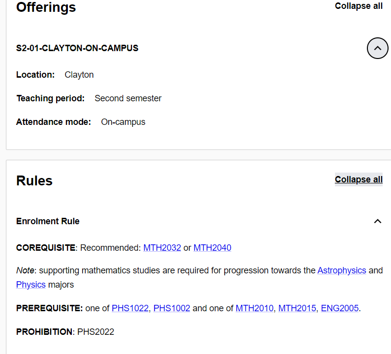
课程介绍：

Quantum mechanics plays a central role in our understanding of fundamental phenomena, primarily in the microscopic domain. It lays the foundation for an understanding of atomic, molecular, condensed matter, nuclear and particle physics.

Quantum Physics量子计算问题集

问题 1. Consider a two-dimensional strip of material of length $L$ and width $W$, placed in a magnetic field perpendicular to the strip and with an electric field established in the direction of the length $L$.
(a) Suppose that the resistivity matrix is given by the classical result
$$
\rho=\left(\begin{array}{cc}
\rho_0 & -\rho_H \
\rho_H & \rho_0
\end{array}\right)
$$
where $\rho_H=B /$ nec is the Hall resistivity and $\rho_0$ is the usual Ohmic resistivity. Find the conductivity matrix, $\sigma=\rho^{-1}$. Write it in the form:
$$
\sigma=\left(\begin{array}{cc}
\sigma_0 & \sigma_H \
-\sigma_H & \sigma_0
\end{array}\right) .
$$
What are $\sigma_0$ and $\sigma_H$ ?
(b) Suppose $B=0$, so the Hall resistivity is zero. Notice that the Ohmic conductivity, $\sigma_0$, is just $1 / \rho_0$. In particular, note that $\sigma_0 \rightarrow \infty$ as $\rho_0 \rightarrow 0$. Now suppose $\rho_H \neq 0$. Show that $\sigma_0 \rightarrow 0$ as $\rho_0 \rightarrow 0$, so it is possible to have both $\sigma_0$ and $\rho_0$ equal to zero

问题 2.

This problem asks you to give a complete presentation of a calculation that is almost the same as one you saw in lecture.

Consider a constant electric field, $\vec{E}=\left(0, E_0, 0\right)$ and a constant magnetic field, $\vec{B}=\left(0,0, B_0\right)$.
(a) Choose an electrostatic potential $\phi$ and a vector potential $\vec{A}$ which describe the $\vec{E}$ and $\vec{B}$ fields, and write the Hamiltonian for a charged particle of mass $m$ and charge $q$ in these fields. Assume that the particle is restricted to move in the $x y$-plane.
(b) What are the allowed energies as a function of $B_0$ and $E_0$ ? Draw a figure to show how the Landau levels (energy levels when $E_0=0$ ) change as $E_0$ increases.

问题 3.

You will see the “standard presentation” of the Aharonov-Bohm effect in lecture, on the day that this problem set is due. The standard presentation has its advantages, and in particular is more general than the presentation you will work through in this problem. However, students often come away from the standard presentation of the Aharonov-Bohm effect thinking that the only way to detect this effect is to do an interference experiment. This is not true, and the purpose of this problem is to disabuse you of this misimpression before you form it.

As Griffiths explains on pages 385-387 (344-345 in 1st Ed.), the Aharonov-Bohm effect modifies the energy eigenvalues of suitably chosen quantum mechanical systems. In this problem, I ask you to work through the same physical example that Griffiths uses, but in a different fashion which makes more use of gauge invariance.

Imagine a particle constrained to move on a circle of radius $b$ (a bead on a wire ring, if you like.) Along the axis of the circle runs a solenoid of radius $a<b$, carrying a magnetic field $\vec{B}=\left(0,0, B_0\right)$. The field inside the solenoid is uniform

and the field outside the solenoid is zero. The setup is depicted in Griffiths’ Fig. 10.10. (10.12 in 1st Ed.)
(a) Construct a vector potential $\vec{A}$ which describes the magnetic field (both inside and outside the solenoid) and which has the form $A_r=A_z=0$ and $A_\phi=\alpha(r)$ for some function $\alpha(r)$. I am using cylindrical coordinates $z, r$, $\phi$.
(b) Since $\vec{\nabla} \times \vec{A}=0$ for $r>a$, it must be possible to write $\vec{A}=\vec{\nabla} f$ in any simply connected region in $r>a$. [This is a theorem in vector calculus.] Show that if we find such an $f$ in the region
$$
r>a \text { and }-\pi+\epsilon<\phi<\pi-\epsilon,
$$
then
$$
f(r, \pi-\epsilon)-f(r,-\pi+\epsilon) \rightarrow \Phi \text { as } \epsilon \rightarrow 0 .
$$
Here, the total magnetic flux is $\Phi=\pi a^2 B_0$. Now find an explicit form for $f$, which is a function only of $\phi$.
(c) Now consider the motion of a “bead on a ring”: write the Schrödinger equation for the particle constrained to move on the circle $r=b$, using the $\vec{A}$ you found in (a). Hint: the answer is given in Griffiths.
(d) Use the $f(\phi)$ found in (b) to gauge transform the Schrödinger equation for $\psi(\phi)$ within the angular region $-\pi+\epsilon<\phi<\pi-\epsilon$ to a Schrödinger equation for a free particle within this angular region. Call the original wave function $\psi(\phi)$ and the gauge-transformed wave function $\psi^{\prime}(\phi)$.
(e) The original wave function $\psi$ must be single-valued for all $\phi$, in particular at $\phi=\pi$. That is, $\psi(\pi-\epsilon)-\psi(-\pi+\epsilon) \rightarrow 0$ and $\frac{\partial \psi}{\partial \phi}(\pi-\epsilon)-\frac{\partial \psi}{\partial \phi}(-\pi+\epsilon) \rightarrow 0$ as $\epsilon \rightarrow 0$. What does this say about the gauge-transformed wave function? I.e., how must $\psi^{\prime}(\pi-\epsilon)$ and $\psi^{\prime}(-\pi+\epsilon)$ be related as $\epsilon \rightarrow 0$ ?
[Hint: because the $f(\phi)$ is not single valued at $\phi=\pi$, the gauge transformed wave function $\psi^{\prime}(\phi)$ is not single valued there either.]
(f) Solve the Schrödinger equation for $\psi^{\prime}$, and find energy eigenstates which satisfy the boundary conditions you derived in (e). What are the allowed energy eigenvalues?
(g) Undo the gauge transformation, and find the energy eigenstates $\psi(\phi)$ in the original gauge. Do the energy eigenvalues in the two gauges differ?
(h) Plot the energy eigenvalues as a function of the enclosed flux, $\Phi$. Show that the energy eigenvalues are periodic functions of $\Phi$ with period $\Phi_0$, where you must determine $\Phi_0$. For what values of $\Phi$ does the enclosed magnetic field have no effect on the spectrum of a particle on a ring? Show that the

Aharonov-Bohm effect can only be used to determine the fractional part of $\Phi / \Phi_0$.
[Note: you have shown that even though the bead on a ring is everywhere in a region in which $\vec{B}=0$, the presence of a nonzero $\vec{A}$ affects the energy eigenvalue spectrum. However, the effect on the energy eigenvalues is determined by $\Phi$, and is therefore gauge invariant. To confirm the gauge invariance of your result, you can compare your answer for the energy eigenvalues to Griffiths’ result, obtained using a different gauge.]

统计代写请认准statistics-lab™. statistics-lab™为您的留学生涯保驾护航。

金融工程代写

金融工程是使用数学技术来解决金融问题。金融工程使用计算机科学、统计学、经济学和应用数学领域的工具和知识来解决当前的金融问题，以及设计新的和创新的金融产品。

非参数统计代写

非参数统计指的是一种统计方法，其中不假设数据来自于由少数参数决定的规定模型；这种模型的例子包括正态分布模型和线性回归模型。

广义线性模型代考

广义线性模型（GLM）归属统计学领域，是一种应用灵活的线性回归模型。该模型允许因变量的偏差分布有除了正态分布之外的其它分布。

术语广义线性模型（GLM）通常是指给定连续和/或分类预测因素的连续响应变量的常规线性回归模型。它包括多元线性回归，以及方差分析和方差分析（仅含固定效应）。

有限元方法代写

有限元方法（FEM）是一种流行的方法，用于数值解决工程和数学建模中出现的微分方程。典型的问题领域包括结构分析、传热、流体流动、质量运输和电磁势等传统领域。

有限元是一种通用的数值方法，用于解决两个或三个空间变量的偏微分方程（即一些边界值问题）。为了解决一个问题，有限元将一个大系统细分为更小、更简单的部分，称为有限元。这是通过在空间维度上的特定空间离散化来实现的，它是通过构建对象的网格来实现的：用于求解的数值域，它有有限数量的点。边界值问题的有限元方法表述最终导致一个代数方程组。该方法在域上对未知函数进行逼近。[1] 然后将模拟这些有限元的简单方程组合成一个更大的方程系统，以模拟整个问题。然后，有限元通过变化微积分使相关的误差函数最小化来逼近一个解决方案。

tatistics-lab作为专业的留学生服务机构，多年来已为美国、英国、加拿大、澳洲等留学热门地的学生提供专业的学术服务，包括但不限于Essay代写，Assignment代写，Dissertation代写，Report代写，小组作业代写，Proposal代写，Paper代写，Presentation代写，计算机作业代写，论文修改和润色，网课代做，exam代考等等。写作范围涵盖高中，本科，研究生等海外留学全阶段，辐射金融，经济学，会计学，审计学，管理学等全球99%专业科目。写作团队既有专业英语母语作者，也有海外名校硕博留学生，每位写作老师都拥有过硬的语言能力，专业的学科背景和学术写作经验。我们承诺100%原创，100%专业，100%准时，100%满意。

随机分析代写

随机微积分是数学的一个分支，对随机过程进行操作。它允许为随机过程的积分定义一个关于随机过程的一致的积分理论。这个领域是由日本数学家伊藤清在第二次世界大战期间创建并开始的。

时间序列分析代写

随机过程，是依赖于参数的一组随机变量的全体，参数通常是时间。随机变量是随机现象的数量表现，其时间序列是一组按照时间发生先后顺序进行排列的数据点序列。通常一组时间序列的时间间隔为一恒定值（如1秒，5分钟，12小时，7天，1年），因此时间序列可以作为离散时间数据进行分析处理。研究时间序列数据的意义在于现实中，往往需要研究某个事物其随时间发展变化的规律。这就需要通过研究该事物过去发展的历史记录，以得到其自身发展的规律。

回归分析代写

多元回归分析渐进（Multiple Regression Analysis Asymptotics）属于计量经济学领域，主要是一种数学上的统计分析方法，可以分析复杂情况下各影响因素的数学关系，在自然科学、社会和经济学等多个领域内应用广泛。

MATLAB代写

MATLAB 是一种用于技术计算的高性能语言。它将计算、可视化和编程集成在一个易于使用的环境中，其中问题和解决方案以熟悉的数学符号表示。典型用途包括：数学和计算算法开发建模、仿真和原型制作数据分析、探索和可视化科学和工程图形应用程序开发，包括图形用户界面构建MATLAB 是一个交互式系统，其基本数据元素是一个不需要维度的数组。这使您可以解决许多技术计算问题，尤其是那些具有矩阵和向量公式的问题，而只需用 C 或 Fortran 等标量非交互式语言编写程序所需的时间的一小部分。MATLAB 名称代表矩阵实验室。MATLAB 最初的编写目的是提供对由 LINPACK 和 EISPACK 项目开发的矩阵软件的轻松访问，这两个项目共同代表了矩阵计算软件的最新技术。MATLAB 经过多年的发展，得到了许多用户的投入。在大学环境中，它是数学、工程和科学入门和高级课程的标准教学工具。在工业领域，MATLAB 是高效研究、开发和分析的首选工具。MATLAB 具有一系列称为工具箱的特定于应用程序的解决方案。对于大多数 MATLAB 用户来说非常重要，工具箱允许您学习和应用专业技术。工具箱是 MATLAB 函数（M 文件）的综合集合，可扩展 MATLAB 环境以解决特定类别的问题。可用工具箱的领域包括信号处理、控制系统、神经网络、模糊逻辑、小波、仿真等。

R语言代写	问卷设计与分析代写
PYTHON代写	回归分析与线性模型代写
MATLAB代写	方差分析与试验设计代写
STATA代写	机器学习/统计学习代写
SPSS代写	计量经济学代写
EVIEWS代写	时间序列分析代写
EXCEL代写	深度学习代写
SQL代写	各种数据建模与可视化代写

PHS2062｜Electromagnetism and optics电磁学和光学蒙纳士大学

Posted on 2023年10月6日2023年10月7日 by statistics-lab

statistics-lab^TM为您提供蒙纳士大学（Monash University）Electromagnetism and optics电磁学和光学澳洲代写代考和辅导服务！

课程介绍：

Electromagnetism and optics fundamentally underpin such modern communication technologies as radio, cellular phones, GPS, Wi-Fi, laser and optical fibres.

1. Electromagnetism: classical electromagnetic theory; Maxwell’s equations; Gauss’s law; Faraday’s law; Ampere-Maxwell law; electric and magnetic fields in vacuum; electrodynamics.

2. Optics: geometric ray tracing; optical cavities; electromagnetic waves; Gaussian beam propagation; multiple-beam interference; polarisation; birefringence.

PHS2062｜Electromagnetism and optics电磁学和光学蒙纳士大学

Mathematical Optimisation for Data Science 数据科学的数学优化案例

问题 1.

(b) Which of the following vector fields could describe an electric field? Say yes or no for each, and give a very brief reason.
(i) $\vec{E}(\vec{r})=x \hat{e}_x-y \hat{e}_y$.
(ii) $\vec{E}(\vec{r})=y \hat{e}_x+x \hat{e}_y$.
(iii) $\vec{E}(\vec{r})=y \hat{e}_x-x \hat{e}_y$.

The curl of an electrostatic field must be zero, but otherwise there is no restriction. So the answer follows as
(i) $\vec{\nabla} \times \vec{E}(\vec{r})=\left(\frac{\partial E_y}{\partial x}-\frac{\partial E_x}{\partial y}\right) \hat{e}_z+\ldots=\overrightarrow{0}$. YES, it describes an electric field.
(ii) $\vec{\nabla} \times \vec{E}(\vec{r})=(1-1) \hat{e}_z=0$. YES, it describes an electric field.
(iii) $\vec{\nabla} \times \vec{E}(\vec{r})=(-1-1) \hat{e}_z=-2 \hat{e}_z$. NO, it does not describe an electric field.

问题 2.

A very long cylindrical object consists of an inner cylinder of radius $a$, which has a uniform charge density $\rho$, and a concentric thin cylinder, of radius $b$, which has an equal but opposite total charge, uniformly distributed on the surface.
(a) Calculate the electric field everywhere.

(a) This problem has enough symmetry to allow a solution by Gauss’s law. In particular, symmetry considerations imply that the electric field will point radially outward, and will have a magnitude that depends only on the distance from the axis. Following Griffiths, we use $s$ for the distance from the $z$-axis, and $\hat{s}$ for a unit vector pointing radially outward from the axis, and of course we choose the $z$-axis to be the axis of the cylindrical object. Then
$$
\vec{E}=E(s) \hat{s} .
$$
To evaluate $E(s)$, we apply Gauss’s law to a Gaussian cylinder of length $\ell$, concentric with the $z$-axis. Then
$$
\oint \vec{E} \cdot \mathrm{d} \vec{a}=\frac{Q_{\text {enc }}}{\epsilon_0}=2 \pi s \ell E(s) .
$$
For $sb$ the enclosed charge is zero, so $E(s)=0$. Putting this together,
$$
\vec{E}=\frac{\rho}{2 \epsilon_0} \begin{cases}s \hat{s} & \text { if } sa .\end{cases}
$$

统计代写请认准statistics-lab™. statistics-lab™为您的留学生涯保驾护航。

金融工程代写

非参数统计代写

非参数统计指的是一种统计方法，其中不假设数据来自于由少数参数决定的规定模型；这种模型的例子包括正态分布模型和线性回归模型。

广义线性模型代考

广义线性模型（GLM）归属统计学领域，是一种应用灵活的线性回归模型。该模型允许因变量的偏差分布有除了正态分布之外的其它分布。

有限元方法代写

随机分析代写

时间序列分析代写

回归分析代写

MATLAB代写

R语言代写	问卷设计与分析代写
PYTHON代写	回归分析与线性模型代写
MATLAB代写	方差分析与试验设计代写
STATA代写	机器学习/统计学习代写
SPSS代写	计量经济学代写
EVIEWS代写	时间序列分析代写
EXCEL代写	深度学习代写
SQL代写	各种数据建模与可视化代写

PHAS0042｜Quantum Mechanics量子力学伦敦大学学院

Posted on 2023年9月27日2023年10月6日 by statistics-lab

如需更详细的代写代考服务，请联系我们的vx客服。无论遇到了什么学科困难，都能帮你完美解决！

STAT0024｜Social Statistics社会统计伦敦大学学院

Posted on 2023年9月25日2023年10月6日 by statistics-lab

statistics-lab^TM为您提供伦敦大学学院（University College London，简称：UCL） STAT0024 Social Statistics社会统计英国代写代考和辅导服务！

课程介绍：

STAT0024 Social Statistics: In-course Assessment 2021-2022 The survey company you work for has been invited by a supermarket chain to bid to design a questionnaire and carry out a sample survey to investigate the views of their current customers about some ideas the chain has for of trying to reduce the amount of packaging, and especially plastic packaging, used in their stores. For example they might stop selling pre-packaged fruit and veg, or offer customers the option of dispensing things like flour or sugar or washing powder into their own containers. There are clear environmental benefits from such ideas, but they will only work if there is take up from the customers.

Social Statistics社会统计作业案例

问题 1.

The binary alloy: A binary alloy (as in $\beta$ brass) consists of $N_A$ atoms of type $A$, and $N_B$ atoms of type $B$. The atoms form a simple cubic lattice, each interacting only with its six nearest neighbors. Assume an attractive energy of $-J \quad(J>0)$ between like neighbors $A-A$ and $B-B$, but a repulsive energy of $+J$ for an $A-B$ pair.

(a) What is the minimum energy configuration, or the state of the system at zero temperature?

The minimum energy configuration has as little A-B bonds as possible. Thus, at zero temperature atoms A and B phase separate, e.g. as indicated below.

问题 2.

(b) Estimate the total interaction energy assuming that the atoms are randomly distributed among the $N$ sites; i.e. each site is occupied independently with probabilities $p_A=N_A / N$ and $p_B=N_B / N$.

In a mixed state, the average energy is obtained from
$$
\begin{aligned}
E & =(\text { number of bonds }) \times(\text { average bond energy }) \
& =3 N \cdot\left(-J p_A^2-J p_B^2+2 J p_A p_B\right) \
& =-3 J N\left(\frac{N_A-N_B}{N}\right)^2
\end{aligned}
$$

问题 3.

From the number of ways of randomly mixing $N_A$ and $N_B$ particles, we obtain the mixing entropy of
$$
S=k_B \ln \left(\frac{N !}{N_{A} ! N_{B} !}\right) .
$$
Using Stirling’s approximation for large $N(\ln N ! \approx N \ln N-N)$, the above expression can be written as
$$
S \approx k_B\left(N \ln N-N_A \ln N_A-N_B \ln N_B\right)=-N k_B\left(p_A \ln p_A+p_B \ln p_B\right) .
$$

统计代写请认准statistics-lab™. statistics-lab™为您的留学生涯保驾护航。

金融工程代写

非参数统计代写

非参数统计指的是一种统计方法，其中不假设数据来自于由少数参数决定的规定模型；这种模型的例子包括正态分布模型和线性回归模型。

广义线性模型代考

广义线性模型（GLM）归属统计学领域，是一种应用灵活的线性回归模型。该模型允许因变量的偏差分布有除了正态分布之外的其它分布。

有限元方法代写

随机分析代写

时间序列分析代写

回归分析代写

MATLAB代写

R语言代写	问卷设计与分析代写
PYTHON代写	回归分析与线性模型代写
MATLAB代写	方差分析与试验设计代写
STATA代写	机器学习/统计学习代写
SPSS代写	计量经济学代写
EVIEWS代写	时间序列分析代写
EXCEL代写	深度学习代写
SQL代写	各种数据建模与可视化代写

PHYS3035｜Electrodynamics and Optics电动力学和光学悉尼大学

Posted on 2023年9月22日2023年10月6日 by statistics-lab

statistics-lab^TM为您提供悉尼大学University of Sydney PHYS3035 Electrodynamics and Optics电动力学和光学澳洲代写代考和辅导服务！

课程介绍：

The development of electrodynamic field theory laid the foundation on which all of modern physics is built, from relativity to quantum field theory. Its application to electromagnetic waves and optics underpins all of modern telecommunications, but also some of the most delicate physics experiments, from gravitational wave detection to quantum computing. This is a core unit in the physics major, which has three components: electrodynamics lectures, optics lectures, and experimental lab. In electrodynamics you will learn to manipulate Maxwell’s equations in their differential form. You will apply the formalism to deriving properties of electromagnetic waves, including the interaction of waves with matter through reflection and absorption. This will lead to optics lectures in which you will investigate aspects of modern optics, using the laser to illustrate the topics covered, in combination with a discussion of the basic optical properties of materials, including the Lorentz model. You will investigate spontaneous and stimulated emission of light, laser rate equations, diffraction, Gaussian beam propagation, anisotropic media and nonlinear optics. You will carry out in-depth experimental investigations into key aspects of electrodynamics, optics, as well as other topics in physics, with expert tutoring.

PHYS3035｜Electrodynamics and Optics电动力学和光学悉尼大学

Electrodynamics and Optics电动力学和光学作业案例

问题 1.

Electrocardiography gathers information about the electrical activity of the heart from measurements of the electric potential at various points on the surface of the heart. This information can be used to estimate the first moment of the effective current source $f(\mathbf{r})$ in (9.55). Specifically, for a body with uniform conductivity $\sigma$ whose volume $V$ is bounded by an insulating medium, prove that the first moment $\Gamma$ of the source strength $f(\mathbf{r})$ is
$$
\Gamma \equiv \int_V d^3 r f(\mathbf{r}) \mathbf{r}=\sigma \int_S d \mathbf{S} \varphi(\mathbf{r}) .
$$
Thus, measurements of electric potential over the surface of the heart give an indication of the integrated strength of the internal current source.

Solution: Begin with (9.55) and focus on one component of the desired moment. This gives
$$
\int_V d^3 r f r_k=-\sigma \int_V d^3 r r_k \nabla^2 \varphi=-\sigma \int_V d^3 r \nabla \cdot\left(r_k \nabla \varphi\right)+\sigma \int_V d^3 r \nabla \varphi \cdot \nabla r_k .
$$
Now apply the divergence theorem to the first term on the far right to get
$$
\Gamma_k \equiv \int_V d^3 r f r_k=-\sigma \int_S d \mathbf{S} \cdot \nabla \varphi r_k+\sigma \int_V d^3 r \nabla \varphi \cdot \nabla r_k .
$$
The insulator boundary condition $\partial \varphi / \partial n=0$ everywhere on $S$ makes the first term on the right vanish. On the other hand, because $\nabla^2 r_k=0$,
$$
\int_V d^3 r \nabla \varphi \cdot \nabla r_k=\int_V d^3 r \nabla \cdot\left(\varphi \nabla r_k\right)-\int_V d^3 r \varphi \nabla^2 r_k=\int_S d \mathbf{S} \cdot \varphi \nabla r_k .
$$
This proves the stated identity because
$$
\Gamma_k=\sigma \int_S d \mathbf{S} \cdot \varphi \nabla r_k=\sigma \int_S d S_k \varphi
$$

问题 2.

How does the force between a charged object and an uncharged simple dielectric depend on the distance $r$ between them? Assume that $r$ is large compared to the size of either object.

Solution: Because the object sizes are small compared to $r$, the variation of the electric field at the position of the dielectric can be taken as $\mathbf{E}_0=\left(Q / 4 \pi \epsilon_0\right) \hat{\mathbf{r}} / r^2$. For the same reason, the force (6.116) on the dielectric can be written in terms of the dipole moment $\mathbf{p}=\int d^3 r \mathbf{P}(\mathbf{r})$ of the dielectric body:
$$
\mathbf{F}=\int d^3 r(\mathbf{P} \cdot \nabla) \mathbf{E}_0 \simeq(\mathbf{p} \cdot \nabla) \mathbf{E}_0
$$

The dielectric is linear, so $\mathbf{p}=\gamma \mathbf{E}_0$ where $\gamma$ is a constant. Therefore, because $\nabla \times \mathbf{E}_0=0$,
$$
\mathbf{F}=\gamma\left(\mathbf{E}_0 \cdot \nabla\right) \mathbf{E}_0=\frac{1}{2} \gamma \nabla\left|\mathbf{E}_0\right|^2 \propto-Q^2 \frac{\hat{\mathbf{r}}}{r^5} .
$$
This force is al ways attractive, independent of the sign of $Q$. The charged object attracts polarization charge of unlike sign and repels polarization charge of like sign. The former is nearer to $Q$ than the latter and thus dominates the net Coulomb interaction.

With other choices for the non-uniform external field $\mathbf{E}_0(\mathbf{r})$, the force $\mathbf{F}=\frac{1}{2} \gamma \nabla\left|\mathbf{E}_0\right|^2$ has been successfully used to sort, position, and transport many different types of minute dielectric bodies, including living cells. This phenomenon is known as dielectrophoresis, from the Greek verb meaning “to bear” or “to carry”.

问题 3.

Let $\mathbf{B}(\mathbf{r})$ be the magnetic field produced by a current density $\mathbf{j}(\mathbf{r})$ which lies entirely inside a spherical volume $V$ of radius $R$. Show that the magnetic moment of $\mathbf{j}(\mathbf{r})$ is
$$
\mathbf{m}=\frac{3}{2 \mu_0} \int_V d^3 r \mathbf{B}(\mathbf{r}) .
$$
This problem is the magnetic analog of Example 4.1, which expressed the electric dipole moment of a charge distribution using a spherical average of the electric field produced by the charge.

Solution: Assume first that $\mathbf{j}(\mathbf{r})$ does not lie entirely inside $V$. If we place the origin of coordinates at the center of $V$, the Biot-Savart law (10.15) gives
$$
\frac{1}{V} \int_V d^3 r \mathbf{B}(\mathbf{r})=-\frac{\mu_0}{4 \pi V} \int d^3 r^{\prime} \mathbf{j}\left(\mathbf{r}^{\prime}\right) \times \int_V d^3 r \frac{\left(\mathbf{r}^{\prime}-\mathbf{r}\right)}{\left|\mathbf{r}^{\prime}-\mathbf{r}\right|^3} .
$$
The $\mathbf{r}$ integral is exactly the “electric” field $\mathbf{E}\left(\mathbf{r}^{\prime}\right)$ due to a uniform charge density $\rho(\mathbf{r})=4 \pi \epsilon_0$. From Gauss’ law or otherwise, this is
$$
\mathbf{E}\left(\mathbf{r}^{\prime}\right)= \begin{cases}\frac{\rho \mathbf{r}^{\prime}}{3 \epsilon_0}=\frac{4 \pi}{3} \mathbf{r}^{\prime} & r^{\prime}R .\end{cases}
$$
Therefore,
$$
\frac{1}{V} \int_V d^3 r \mathbf{B}(\mathbf{r})=\frac{\mu_0}{3 V} \int_{r^{\prime} \leq R} d^3 r^{\prime} \mathbf{r}^{\prime} \times \mathbf{j}\left(\mathbf{r}^{\prime}\right)-\frac{\mu_0}{4 \pi} \int_{r^{\prime}>R} d^3 r^{\prime} \frac{\mathbf{j}\left(\mathbf{r}^{\prime}\right) \times \mathbf{r}^{\prime}}{r^{\prime 3}}
$$

the first integral on the right side of this equation is proportional to $\mathbf{m}{\text {in }}$, the magnetic moment due to the part of $\mathbf{j}$ which lies inside $V$. The second integral is the Biot-Savart magnetic field at the origin, $\mathbf{B}{\text {out }}(0)$, due to that part of $\mathbf{j}$ which lies outside $V$. Therefore,
$$
\frac{1}{V} \int_V d^3 r \mathbf{B}(\mathbf{r})=\frac{2}{3} \mu_0 \frac{\mathbf{m}{\text {in }}}{V}+\mathbf{B}{\text {out }}(0) .
$$
This formula reduces to the advertised result if all of $\mathbf{j}(\mathbf{r})$ is contained in $V$. On the other hand, if none of the current is contained in $V$,
$$
\mathbf{B}(0)=\frac{1}{V} \int d^3 r \mathbf{B}(\mathbf{r})
$$

统计代写请认准statistics-lab™. statistics-lab™为您的留学生涯保驾护航。

金融工程代写

非参数统计代写

非参数统计指的是一种统计方法，其中不假设数据来自于由少数参数决定的规定模型；这种模型的例子包括正态分布模型和线性回归模型。

广义线性模型代考

广义线性模型（GLM）归属统计学领域，是一种应用灵活的线性回归模型。该模型允许因变量的偏差分布有除了正态分布之外的其它分布。

有限元方法代写

随机分析代写

时间序列分析代写

回归分析代写

MATLAB代写

R语言代写	问卷设计与分析代写
PYTHON代写	回归分析与线性模型代写
MATLAB代写	方差分析与试验设计代写
STATA代写	机器学习/统计学习代写
SPSS代写	计量经济学代写
EVIEWS代写	时间序列分析代写
EXCEL代写	深度学习代写
SQL代写	各种数据建模与可视化代写

物理代写|量子场论代写Quantum field theory代考|PHYC90008

Posted on 2023年8月30日2023年8月30日 by statistics-lab

如果你也在怎样代写量子场论Quantum field theory 这个学科遇到相关的难题，请随时右上角联系我们的24/7代写客服。量子场论Quantum field theory提供了一套极其强大的计算方法，但尚未发现任何基本限制。它导致了科学史上理论预测和实验数据之间最奇妙的一致。

量子场论Quantum field theory对我们的宇宙的本质，以及其他可能的自洽宇宙的本质，提供了深刻而深刻的见解。另一方面，这个主题是一团糟。它的基础是脆弱的，它可能是荒谬的复杂，而且很可能是不完整的。通常有很多方法可以解决同样的问题，有时没有一个是特别令人满意的。这给这个主题的介绍的设计和呈现留下了巨大的挑战。

statistics-lab™ 为您的留学生涯保驾护航在代写量子场论Quantum field theory方面已经树立了自己的口碑, 保证靠谱, 高质且原创的统计Statistics代写服务。我们的专家在代写量子场论Quantum field theory代写方面经验极为丰富，各种代写量子场论Quantum field theory相关的作业也就用不着说。

物理代写|量子场论代写Quantum field theory代考|PHYC90008

物理代写|量子场论代写Quantum field theory代考|Classical electrodynamics

We would expect the Hamiltonian of a system of moving charges, such as an atom, in an electromagnetic field to consist of three parts: a part referring to matter (i.e. the charges), a part referring to the electromagnetic field and a part describing the interaction between matter and field.

For a system of point masses $m_i, i=1, \ldots, N$, with charges $e_i$ and position coordinates $\mathbf{r}i$, the Hamiltonian is $$ H{\mathrm{m}}=\sum_i \frac{\mathbf{p}i^2}{2 m_i}+H{\mathrm{C}}
$$
where $H_{\mathrm{C}}$ is the Coulomb interaction
$$
H_{\mathrm{C}} \equiv \frac{1}{2} \sum_{\substack{i, j \(i \neq j)}} \frac{e_i e_j}{4 \pi\left|\mathbf{r}_i-\mathbf{r}_j\right|}
$$
and $\mathbf{p}_i=m_i \mathrm{~d} \mathbf{r}_i / \mathrm{d} t$ is the kinetic momentum of the $i$ th particle. This is the usual Hamiltonian of atomic physics, for example.

The electromagnetic field in interaction with charges is described by Maxwell’s equations [Eqs. (1.1)]. We continue to use the Coulomb gauge, $\boldsymbol{\nabla} \cdot \mathbf{A}=0$, so that the electric field (1.2) decomposes into transverse and longitudinal fields
$$
\mathbf{E}=\mathbf{E}{\mathbf{T}}+\mathbf{E}{\mathbf{L}},
$$
where
$$
\mathbf{E}{\mathbf{T}}=-\frac{1}{c} \frac{\partial \mathbf{A}}{\partial t}, \quad \mathbf{E}{\mathbf{L}}=-\nabla \phi
$$

物理代写|量子场论代写Quantum field theory代考|Quantum electrodynamics

The quantization of the system described by the Hamiltonian (1.63) is carried out by subjecting the particles’ coordinates $\mathbf{r}i$ and canonically conjugate momenta $\mathbf{p}_i$ to the usual commutation relations (e.g. in the coordinate representation $\mathbf{p}_i \rightarrow i \hbar \boldsymbol{\nabla}_i$ ), and quantizing the radiation field, as in Section 1.2.3. The longitudinal electric field $\mathbf{E}{\mathbf{L}}$ does not pro

The eigenstates of $H_0$ are again of the form
$$
\left|A, \ldots n_r(\mathbf{k}) \ldots\right\rangle=|A\rangle\left|\ldots n_r(\mathbf{k}) \ldots\right\rangle,
$$
with $|A\rangle$ and $\left|\ldots n_r(\mathbf{k}) \ldots\right\rangle$ eigenstates of $H_{\mathrm{m}}$ and $H_{\mathrm{rad}}$.
Compared with the electric dipole interaction (1.40), the interaction (1.62) differs in that it contains a term quadratic in the vector potential. This results in two-photon processes in first-order perturbation theory (i.e. emission or absorption of two photons or scattering). In addition, the first term in (1.62) contains magnetic interactions and higher-order effects due to the spatial variation of $\mathbf{A}(\mathbf{x}, t)$, which are absent from the electric dipole interaction (1.40). These aspects are illustrated in the applications to radiative transitions and Thomson scattering which follow.

vide any additional degrees of freedom, being completely determined via the first Maxwell equation $\boldsymbol{\nabla} \cdot \mathbf{E}_{\mathbf{L}}=\rho$ by the charges.

The interaction $H_{\mathrm{I}}$ in Eq, (1.63) is usually treated as a perturbation which causes transitions between the states of the non-interacting Hamiltonian
$$
H_0=H_{\mathrm{m}}+H_{\text {rad }} \text {. }
$$

量子场论代考

物理代写|量子场论代写Quantum field theory代考|Classical electrodynamics

我们期望在电磁场中运动电荷系统(如原子)的哈密顿量由三部分组成:一部分涉及物质(即电荷)，一部分涉及电磁场，另一部分描述物质与场之间的相互作用。

对于质点系统$m_i, i=1, \ldots, N$，电荷为$e_i$，位置坐标为$\mathbf{r}i$，哈密顿量为$$ H{\mathrm{m}}=\sum_i \frac{\mathbf{p}i^2}{2 m_i}+H{\mathrm{C}}
$$
库仑相互作用$H_{\mathrm{C}}$在哪里
$$
H_{\mathrm{C}} \equiv \frac{1}{2} \sum_{\substack{i, j (i \neq j)}} \frac{e_i e_j}{4 \pi\left|\mathbf{r}_i-\mathbf{r}_j\right|}
$$
$\mathbf{p}_i=m_i \mathrm{~d} \mathbf{r}_i / \mathrm{d} t$是第$i$个粒子的动能。例如，这是原子物理学中常用的哈密顿量。

电磁场与电荷的相互作用用麦克斯韦方程描述。(1.1)]。我们继续使用库仑规$\boldsymbol{\nabla} \cdot \mathbf{A}=0$，使电场(1.2)分解为横向场和纵向场
$$
\mathbf{E}=\mathbf{E}{\mathbf{T}}+\mathbf{E}{\mathbf{L}},
$$
在哪里
$$
\mathbf{E}{\mathbf{T}}=-\frac{1}{c} \frac{\partial \mathbf{A}}{\partial t}, \quad \mathbf{E}{\mathbf{L}}=-\nabla \phi
$$

物理代写|量子场论代写Quantum field theory代考|Quantum electrodynamics

由哈密顿量(1.63)描述的系统的量子化是通过使粒子的坐标$\mathbf{r}i$和标准共轭动量$\mathbf{p}_i$服从通常的对易关系(例如在坐标表示$\mathbf{p}_i \rightarrow i \hbar \boldsymbol{\nabla}_i$中)，并将辐射场量子化来实现的，如第1.2.3节所述。纵向电场$\mathbf{E}{\mathbf{L}}$不亲

$H_0$的特征态也是这种形式
$$
\left|A, \ldots n_r(\mathbf{k}) \ldots\right\rangle=|A\rangle\left|\ldots n_r(\mathbf{k}) \ldots\right\rangle,
$$
具有$|A\rangle$和$\left|\ldots n_r(\mathbf{k}) \ldots\right\rangle$的特征态$H_{\mathrm{m}}$和$H_{\mathrm{rad}}$。
与电偶极相互作用(1.40)相比，相互作用(1.62)的不同之处在于它在矢量势中包含了一个二次项。这导致了一阶微扰理论中的双光子过程(即两个光子的发射或吸收或散射)。此外，(1.62)中的第一项包含磁相互作用和高阶效应，这是由于$\mathbf{A}(\mathbf{x}, t)$的空间变化，这在电偶极相互作用(1.40)中不存在。这些方面将在随后的辐射跃迁和汤姆逊散射的应用中加以说明。

没有任何额外的自由度，完全由第一个麦克斯韦方程$\boldsymbol{\nabla} \cdot \mathbf{E}_{\mathbf{L}}=\rho$由电荷决定。

Eq，(1.63)中的相互作用$H_{\mathrm{I}}$通常被视为引起非相互作用哈密顿量状态之间转换的扰动
$$
H_0=H_{\mathrm{m}}+H_{\text {rad }} \text {. }
$$

物理代写|量子场论代写Quantum field theory代考请认准statistics-lab™

统计代写请认准statistics-lab™. statistics-lab™为您的留学生涯保驾护航。

金融工程代写

非参数统计代写

非参数统计指的是一种统计方法，其中不假设数据来自于由少数参数决定的规定模型；这种模型的例子包括正态分布模型和线性回归模型。

广义线性模型代考

广义线性模型（GLM）归属统计学领域，是一种应用灵活的线性回归模型。该模型允许因变量的偏差分布有除了正态分布之外的其它分布。

有限元方法代写

随机分析代写

时间序列分析代写

回归分析代写

MATLAB代写

R语言代写	问卷设计与分析代写
PYTHON代写	回归分析与线性模型代写
MATLAB代写	方差分析与试验设计代写
STATA代写	机器学习/统计学习代写
SPSS代写	计量经济学代写
EVIEWS代写	时间序列分析代写
EXCEL代写	深度学习代写
SQL代写	各种数据建模与可视化代写

物理代写|量子场论代写Quantum field theory代考|PHYS4125

Posted on 2023年8月30日2023年8月30日 by statistics-lab

物理代写|量子场论代写Quantum field theory代考|The quantized radiation field

The harmonic oscillator results we have derived can at once be applied to the radiation field. Its Hamiltonian, Eq. (1.18), is a superposition of independent harmonic oscillator Hamiltonians (1.20), one for each mode of the radiation field. [The order of the factors in (1.18) is not significant and can be changed, since the $a_{\mathrm{r}}$ and $a_r^*$ are classical amplitudes.] We therefore introduce commutation relations analogous to Eq. (1.19)
$$
\left.\begin{array}{l}
{\left[a_r(\mathbf{k}), a_s^{\dagger}\left(\mathbf{k}^{\prime}\right)\right]=\delta_{r s} \delta_{\mathbf{k} \mathbf{k}^{\prime}}} \
{\left[a_r(\mathbf{k}), a_s\left(\mathbf{k}^{\prime}\right)\right]=\left[a_r^{\dagger}(\mathbf{k}), a_s^{\dagger}\left(\mathbf{k}^{\prime}\right)\right]=0}
\end{array}\right}
$$
and write the Hamiltonian (1.18) as
$$
H_{\mathrm{rad}}=\sum_{\mathbf{k}} \sum_r \hbar \omega_{\mathbf{k}}\left(a_r^{\dagger}(\mathbf{k}) a_r(\mathbf{k})+\frac{1}{2}\right) .
$$
The operators
$$
N_r(\mathbf{k})=a_r^{\dagger}(\mathbf{k}) a_r(\mathbf{k})
$$
then have eigenvalues $n_r(\mathbf{k})=0,1,2, \ldots$, and eigenfunctions of the form (1.25)
$$
\left|n_r(\mathbf{k})\right\rangle=\frac{\left[a_r^{\dagger}(\mathbf{k})\right]^{n_r(\mathbf{k})}}{\sqrt{n_r(\mathbf{k}) !}}|0\rangle .
$$
The eigenfunctions of the radiation Hamiltonian (1.30) are products of such states, i.e.
$$
\left|\ldots n_r(\mathbf{k}) \ldots\right\rangle=\prod_{\mathbf{k}i} \prod{r_i}\left|n_{r_i}\left(\mathbf{k}i\right)\right\rangle $$ with energy $$ \sum{\mathbf{k}} \sum_r \hbar \omega_{\mathbf{k}}\left(n_r(\mathbf{k})+\frac{1}{2}\right)
$$

物理代写|量子场论代写Quantum field theory代考|The Electric Dipole Interaction

In the last section we quantized the radiation field. Since the occupation number operators $a_r^{\dagger}(\mathbf{k}) a_r(\mathbf{k})$ commute with the radiation Hamiltonian (1.37), the occupation numbers $n_r(\mathbf{k})$ are constants of the motion for the free field. For anything ‘to happen’ requires interactions with charges and currents so that photons can be absorbed, emitted or scattered.

The complete description of the interaction of a system of charges (for example, an atom or a nucleus) with an electromagnetic field is very complicated. In this section we shall consider the simpler and, in practice, important special case of the interaction occurring via the electric dipole moment of the system of charges. The more complete (but still noncovariant) treatment of Section 1.4 will justify some of the points asserted in this section.
We shall consider a system of $N$ charges $e_1, e_2, \ldots, e_N$ which can be described nonrelativistically, i.e. the position of $\mathrm{e}i, i=1, \ldots, N$, at time $t$ is classically given by $\mathbf{r}_i=\mathbf{r}_i(t)$. We consider transitions between def inite initial and final states of the system (e.g. between two states of an atom). The transitions are brought about by the electric dipole interaction if two approximations are valid. Firstly it is permissible to neglect the interactions with the magnetic field. Secondly, one may neglect the spatial variation of the electric radiation field, causing the transitions, across the system of charges (e.g. across the atom). Under these conditions the electric field $$ \mathbf{E}{\mathrm{T}}(\mathbf{r}, t)=-\frac{1}{c} \frac{\partial \mathbf{A}(\mathbf{r}, t)}{\partial t},
$$
resulting from the transverse vector potential (1.38) of the radiation field (we are again using the Coulomb gauge $\boldsymbol{\nabla} \cdot \mathbf{A}=0$ ), can be calculated at one point somewhere inside the system of charges, instead of at the position of each charge. ${ }^6$ Taking this point as the origin of coordinates $\mathbf{r}=0$, we obtain for the interaction causing transitions, the electric dipole interaction $H_{\mathrm{I}}$ given by
$$
H_{\mathrm{I}}=-\mathbf{D} \cdot \mathbf{E}_{\mathrm{T}}(0, t)
$$
where the electric dipole moment is defined by
$$
\mathbf{D}=\sum e_i \mathbf{r}_i
$$

量子场论代考

物理代写|量子场论代写Quantum field theory代考|The quantized radiation field

我们所导出的谐振子结果可以立即应用于辐射领域。它的哈密顿量Eq.(1.18)是独立谐振子哈密顿量(1.20)的叠加，每个模式对应一个辐射场。(1.18)中因子的顺序不显著，可以改变，因为$a_{\mathrm{r}}$和$a_r^*$是经典振幅。因此，我们引入类似于式(1.19)的交换关系。
$$
\left.\begin{array}{l}
{\left[a_r(\mathbf{k}), a_s^{\dagger}\left(\mathbf{k}^{\prime}\right)\right]=\delta_{r s} \delta_{\mathbf{k} \mathbf{k}^{\prime}}} \
{\left[a_r(\mathbf{k}), a_s\left(\mathbf{k}^{\prime}\right)\right]=\left[a_r^{\dagger}(\mathbf{k}), a_s^{\dagger}\left(\mathbf{k}^{\prime}\right)\right]=0}
\end{array}\right}
$$
把哈密顿式(1.18)写成
$$
H_{\mathrm{rad}}=\sum_{\mathbf{k}} \sum_r \hbar \omega_{\mathbf{k}}\left(a_r^{\dagger}(\mathbf{k}) a_r(\mathbf{k})+\frac{1}{2}\right) .
$$
算子
$$
N_r(\mathbf{k})=a_r^{\dagger}(\mathbf{k}) a_r(\mathbf{k})
$$
则有特征值$n_r(\mathbf{k})=0,1,2, \ldots$，特征函数的形式为(1.25)
$$
\left|n_r(\mathbf{k})\right\rangle=\frac{\left[a_r^{\dagger}(\mathbf{k})\right]^{n_r(\mathbf{k})}}{\sqrt{n_r(\mathbf{k}) !}}|0\rangle .
$$
辐射哈密顿量(1.30)的本征函数是这些状态的乘积，即。
$$
\left|\ldots n_r(\mathbf{k}) \ldots\right\rangle=\prod_{\mathbf{k}i} \prod{r_i}\left|n_{r_i}\left(\mathbf{k}i\right)\right\rangle $$ with energy $$ \sum{\mathbf{k}} \sum_r \hbar \omega_{\mathbf{k}}\left(n_r(\mathbf{k})+\frac{1}{2}\right)
$$

物理代写|量子场论代写Quantum field theory代考|The Electric Dipole Interaction

在上一节中，我们对辐射场进行了量子化。由于占用数运算符$a_r^{\dagger}(\mathbf{k}) a_r(\mathbf{k})$与辐射哈密顿量(1.37)互换，因此占用数$n_r(\mathbf{k})$是自由场运动的常数。任何“发生”的事情都需要与电荷和电流相互作用，这样光子才能被吸收、发射或散射。

电荷系统(例如原子或原子核)与电磁场相互作用的完整描述是非常复杂的。在本节中，我们将考虑通过电荷系统的电偶极矩发生的相互作用的更简单、在实践中更重要的特殊情况。对1.4节的更完整(但仍然是非协变的)处理将证明本节中断言的一些观点是正确的。
我们将考虑一个由$N$电荷$e_1, e_2, \ldots, e_N$组成的系统，它可以用非相对论性来描述，即$\mathrm{e}i, i=1, \ldots, N$在时间$t$时的位置经典地由$\mathbf{r}i=\mathbf{r}_i(t)$给出。我们考虑系统的确定初始状态和最终状态之间的转换(例如，在原子的两个状态之间)。如果两个近似都成立，则跃迁是由电偶极相互作用引起的。首先，可以忽略与磁场的相互作用。其次，人们可以忽略电辐射场的空间变化，它会引起整个电荷系统(例如原子)的跃迁。在这些条件下电场$$ \mathbf{E}{\mathrm{T}}(\mathbf{r}, t)=-\frac{1}{c} \frac{\partial \mathbf{A}(\mathbf{r}, t)}{\partial t}, $$ 由辐射场的横向矢量势(1.38)产生(我们再次使用库仑规$\boldsymbol{\nabla} \cdot \mathbf{A}=0$)，可以在电荷系统内的某个点计算，而不是在每个电荷的位置。${ }^6$以该点为坐标原点$\mathbf{r}=0$，我们得到引起跃迁的相互作用，电偶极相互作用$H{\mathrm{I}}$由
$$
H_{\mathrm{I}}=-\mathbf{D} \cdot \mathbf{E}_{\mathrm{T}}(0, t)
$$
电偶极矩的定义是什么
$$
\mathbf{D}=\sum e_i \mathbf{r}_i
$$

统计代写请认准statistics-lab™. statistics-lab™为您的留学生涯保驾护航。

金融工程代写

非参数统计代写

非参数统计指的是一种统计方法，其中不假设数据来自于由少数参数决定的规定模型；这种模型的例子包括正态分布模型和线性回归模型。

广义线性模型代考

广义线性模型（GLM）归属统计学领域，是一种应用灵活的线性回归模型。该模型允许因变量的偏差分布有除了正态分布之外的其它分布。

有限元方法代写

随机分析代写

时间序列分析代写

回归分析代写

MATLAB代写

R语言代写	问卷设计与分析代写
PYTHON代写	回归分析与线性模型代写
MATLAB代写	方差分析与试验设计代写
STATA代写	机器学习/统计学习代写
SPSS代写	计量经济学代写
EVIEWS代写	时间序列分析代写
EXCEL代写	深度学习代写
SQL代写	各种数据建模与可视化代写

物理代写|量子场论代写Quantum field theory代考|FYS4170

Posted on 2023年8月30日2023年8月30日 by statistics-lab

物理代写|量子场论代写Quantum field theory代考|The classical field

Classical electromagnetic theory is summed up in Maxwell’s equations. In the presence of a charge density $\rho(\mathbf{x}, t)$ and a current density $\mathbf{j}(\mathbf{x}, \mathrm{t})$, the electric and magnetic fields $\mathbf{E}$ and $\mathbf{B}$ satisfy the equations
$$
\begin{aligned}
\boldsymbol{\nabla} \cdot \mathbf{E} & =\rho \
\boldsymbol{\nabla} \wedge \mathbf{B} & =\frac{1}{c} \mathbf{j}+\frac{1}{c} \frac{\partial \mathbf{E}}{\partial t} \
\boldsymbol{\nabla} \cdot \mathbf{B} & =0 \
\boldsymbol{\nabla} \wedge \mathbf{E} & =-\frac{1}{c} \frac{\partial \mathbf{B}}{\partial t}
\end{aligned}
$$
where, as throughout this book, rationalized Gaussian (c.g.s.) units are being used. ${ }^1$
From the second pair of Maxwell’s equations [Eqs. (1.1c) and (1.1d)] follows the existence of scalar and vector potentials $\phi(\mathbf{x}, t)$ and $\mathbf{A}(\mathbf{x}, t)$, defined by
$$
\mathbf{B}=\boldsymbol{\nabla} \wedge \mathbf{A}, \quad \mathbf{E}=-\boldsymbol{\nabla} \phi-\frac{1}{c} \frac{\partial \mathbf{A}}{\partial t} .
$$
Eqs. (1.2) do not determine the potentials uniquely, since for an arbitrary function $f(\mathbf{x}, t)$ the transformation
$$
\phi \rightarrow \phi^{\prime}=\phi+\frac{1}{c} \frac{\partial f}{\partial t}, \quad \mathbf{A} \rightarrow \mathbf{A}^{\prime}=\mathbf{A}-\nabla f
$$
leaves the fields $\mathbf{E}$ and $\mathbf{B}$ unaltered. The transformation (1.3) is known as a gauge transformation of the second kind. Since all observable quantities can be expressed in terms of $\mathbf{E}$ and $\mathbf{B}$, it is a fundamental requirement of any theory formulated in terms of potentials that it is gauge-invariant, i.e. that the predictions for observable quantities are invariant under such gauge transformations.

Expressed in terms of the potentials, the second pair of Maxwell’s equations [Eqs. (1.1c) and (1.1d)] are satisfied automatically, while the first pair [Eqs. (1.1a) and (1.1b)] become
$$
\begin{gathered}
-\nabla^2 \phi-\frac{1}{c} \frac{\partial}{\partial t}(\boldsymbol{\nabla} \cdot \mathbf{A})=\square \phi-\frac{1}{c} \frac{\partial}{\partial t}\left(\frac{1}{c} \frac{\partial \phi}{\partial t}+\nabla \cdot \mathbf{A}\right)=\rho \
\square \mathbf{A}+\boldsymbol{\nabla}\left(\frac{1}{c} \frac{\partial \phi}{\partial t}+\nabla \cdot \mathbf{A}\right)=\frac{1}{c} \mathbf{j}
\end{gathered}
$$
where
$$
\square \equiv \frac{1}{c^2} \frac{\partial^2}{\partial t^2}-\nabla^2
$$

物理代写|量子场论代写Quantum field theory代考|Harmonic oscillator

The harmonic oscillator Hamiltonian is, in an obvious notation,
$$
H_{\mathrm{osc}}=\frac{p^2}{2 m}+\frac{1}{2} m \omega^2 q^2,
$$
with $q$ and $p$ satisf ying the commutation relation $[q, p]=\mathrm{i} \hbar$. We introduce the operators
$$
\left.\begin{array}{c}
a \
a^{\dagger}
\end{array}\right}=\frac{1}{(2 \hbar m \omega)^{1 / 2}}(m \omega q \pm \mathrm{i} p) .
$$
These satisfy the commutation relation
$$
\left[a, a^{\dagger}\right]=1,
$$
and the Hamiltonian expressed in terms of $a$ and $a^{\dagger}$ becomes:
$$
H_{\mathrm{osc}}=\frac{1}{2} \hbar \omega\left(a^{\dagger} a+a a^{\dagger}\right)=\hbar \omega\left(a^{\dagger} a+\frac{1}{2}\right) .
$$
This is essentially the operator
$$
N \equiv a^{\dagger} a,
$$

which is positive definite, i.e. for any state $|\Psi\rangle$
$$
\langle\Psi|N| \Psi\rangle=\left\langle\Psi\left|a^{\dagger} a\right| \Psi\right\rangle=\langle a \Psi \mid a \Psi\rangle \geq 0 .
$$
Hence, $N$ possesses a lowest non-negative eigenvalue
$$
\alpha_0 \geq 0 \text {. }
$$
It follows from the eigenvalue equation
$$
N|\alpha\rangle=\alpha|\alpha\rangle
$$
and Eq. (1.19) that
$$
N a|\alpha\rangle=(\alpha-1) a|\alpha\rangle, \quad N a^{\dagger}|\alpha\rangle=(\alpha+1) a^{\dagger}|\alpha\rangle,
$$
i.e. $a|\alpha\rangle$ and $a^{\dagger}|\alpha\rangle$ are eigenfunctions of $N$ belonging to the eigenvalues $(\alpha-1)$ and $(\alpha+1)$, respectively. Since $\alpha_0$ is the lowest eigenvalue we must have
$$
a\left|\alpha_0\right\rangle=0
$$
and since
$$
a^{\dagger} a\left|\alpha_0\right\rangle=\alpha_0\left|\alpha_0\right\rangle
$$
Eq. (1.23) implies $\alpha_0=0$. It follows from Eqs. (1.19) and (1.22) that the eigenvalues of $N$ are the integers $n=0,1,2, \ldots$, and that if $\langle n \mid n\rangle=1$, then the states $|n \pm 1\rangle$, defined by
$$
a|n\rangle=n^{1 / 2}|n-1\rangle, \quad a^{\dagger}|n\rangle=(n+1)^{1 / 2}|n+1\rangle,
$$
are also normed to unity. If $\langle 0 \mid 0\rangle=1$, the normed eigenf unctions of $N$ are
$$
|n\rangle=\frac{\left(a^{\dagger}\right)^n}{\sqrt{n !}}|0\rangle, \quad n=0,1,2, \ldots
$$

量子场论代考

物理代写|量子场论代写Quantum field theory代考|The classical field

经典电磁理论可归纳为麦克斯韦方程组。当电荷密度$\rho(\mathbf{x}, t)$和电流密度$\mathbf{j}(\mathbf{x}, \mathrm{t})$存在时，电场$\mathbf{E}$和磁场$\mathbf{B}$满足方程
$$
\begin{aligned}
\boldsymbol{\nabla} \cdot \mathbf{E} & =\rho \
\boldsymbol{\nabla} \wedge \mathbf{B} & =\frac{1}{c} \mathbf{j}+\frac{1}{c} \frac{\partial \mathbf{E}}{\partial t} \
\boldsymbol{\nabla} \cdot \mathbf{B} & =0 \
\boldsymbol{\nabla} \wedge \mathbf{E} & =-\frac{1}{c} \frac{\partial \mathbf{B}}{\partial t}
\end{aligned}
$$
在这里，贯穿本书，理性化高斯(c.g.s)单位被使用。${ }^1$
从第二对麦克斯韦方程方程和(1.1d)]表示标量势$\phi(\mathbf{x}, t)$和矢量势$\mathbf{A}(\mathbf{x}, t)$的存在，定义为
$$
\mathbf{B}=\boldsymbol{\nabla} \wedge \mathbf{A}, \quad \mathbf{E}=-\boldsymbol{\nabla} \phi-\frac{1}{c} \frac{\partial \mathbf{A}}{\partial t} .
$$
等式。(1.2)不确定唯一的势，因为对于任意函数$f(\mathbf{x}, t)$变换
$$
\phi \rightarrow \phi^{\prime}=\phi+\frac{1}{c} \frac{\partial f}{\partial t}, \quad \mathbf{A} \rightarrow \mathbf{A}^{\prime}=\mathbf{A}-\nabla f
$$
保持字段$\mathbf{E}$和$\mathbf{B}$不变。变换(1.3)被称为第二类规范变换。由于所有可观测量都可以用$\mathbf{E}$和$\mathbf{B}$来表示，因此任何用势表示的理论的基本要求是它是规范不变的，即在这种规范变换下对可观测量的预测是不变的。

用势来表示，第二对麦克斯韦方程[方程]。(1.1c)和(1.1d)]自动满足，而第一对[式。(1.1a)和(1.1b)]变成
$$
\begin{gathered}
-\nabla^2 \phi-\frac{1}{c} \frac{\partial}{\partial t}(\boldsymbol{\nabla} \cdot \mathbf{A})=\square \phi-\frac{1}{c} \frac{\partial}{\partial t}\left(\frac{1}{c} \frac{\partial \phi}{\partial t}+\nabla \cdot \mathbf{A}\right)=\rho \
\square \mathbf{A}+\boldsymbol{\nabla}\left(\frac{1}{c} \frac{\partial \phi}{\partial t}+\nabla \cdot \mathbf{A}\right)=\frac{1}{c} \mathbf{j}
\end{gathered}
$$
在哪里
$$
\square \equiv \frac{1}{c^2} \frac{\partial^2}{\partial t^2}-\nabla^2
$$

物理代写|量子场论代写Quantum field theory代考|Harmonic oscillator

谐振子的哈密顿量，用一个明显的符号表示，
$$
H_{\mathrm{osc}}=\frac{p^2}{2 m}+\frac{1}{2} m \omega^2 q^2,
$$
与$q$和$p$满足交换关系$[q, p]=\mathrm{i} \hbar$。我们引入算子
$$
\left.\begin{array}{c}
a \
a^{\dagger}
\end{array}\right}=\frac{1}{(2 \hbar m \omega)^{1 / 2}}(m \omega q \pm \mathrm{i} p) .
$$
它们满足交换关系
$$
\left[a, a^{\dagger}\right]=1,
$$
用$a$和$a^{\dagger}$表示的哈密顿量变为:
$$
H_{\mathrm{osc}}=\frac{1}{2} \hbar \omega\left(a^{\dagger} a+a a^{\dagger}\right)=\hbar \omega\left(a^{\dagger} a+\frac{1}{2}\right) .
$$
这就是算子
$$
N \equiv a^{\dagger} a,
$$

哪个是正定的，对于任何状态$|\Psi\rangle$
$$
\langle\Psi|N| \Psi\rangle=\left\langle\Psi\left|a^{\dagger} a\right| \Psi\right\rangle=\langle a \Psi \mid a \Psi\rangle \geq 0 .
$$
因此，$N$具有最低的非负特征值
$$
\alpha_0 \geq 0 \text {. }
$$
它由特征值方程推导出来
$$
N|\alpha\rangle=\alpha|\alpha\rangle
$$
由式(1.19)可知
$$
N a|\alpha\rangle=(\alpha-1) a|\alpha\rangle, \quad N a^{\dagger}|\alpha\rangle=(\alpha+1) a^{\dagger}|\alpha\rangle,
$$
即$a|\alpha\rangle$和$a^{\dagger}|\alpha\rangle$分别是$N$的特征函数，分别属于特征值$(\alpha-1)$和$(\alpha+1)$。因为$\alpha_0$是最小的特征值
$$
a\left|\alpha_0\right\rangle=0
$$
既然
$$
a^{\dagger} a\left|\alpha_0\right\rangle=\alpha_0\left|\alpha_0\right\rangle
$$
Eq.(1.23)表示$\alpha_0=0$。由等式可知。(1.19)和式(1.22)可知$N$的特征值是整数$n=0,1,2, \ldots$，如果$\langle n \mid n\rangle=1$，则状态$|n \pm 1\rangle$，定义为
$$
a|n\rangle=n^{1 / 2}|n-1\rangle, \quad a^{\dagger}|n\rangle=(n+1)^{1 / 2}|n+1\rangle,
$$
也习惯于团结。若$\langle 0 \mid 0\rangle=1$，则$N$的赋范特征函数为
$$
|n\rangle=\frac{\left(a^{\dagger}\right)^n}{\sqrt{n !}}|0\rangle, \quad n=0,1,2, \ldots
$$

统计代写请认准statistics-lab™. statistics-lab™为您的留学生涯保驾护航。

金融工程代写

非参数统计代写

非参数统计指的是一种统计方法，其中不假设数据来自于由少数参数决定的规定模型；这种模型的例子包括正态分布模型和线性回归模型。

广义线性模型代考

广义线性模型（GLM）归属统计学领域，是一种应用灵活的线性回归模型。该模型允许因变量的偏差分布有除了正态分布之外的其它分布。

有限元方法代写

随机分析代写

时间序列分析代写

回归分析代写

MATLAB代写

R语言代写	问卷设计与分析代写
PYTHON代写	回归分析与线性模型代写
MATLAB代写	方差分析与试验设计代写
STATA代写	机器学习/统计学习代写
SPSS代写	计量经济学代写
EVIEWS代写	时间序列分析代写
EXCEL代写	深度学习代写
SQL代写	各种数据建模与可视化代写

物理代写|热力学代写thermodynamics代考|MENG3401

Posted on 2023年8月30日2023年8月30日 by statistics-lab

如果你也在怎样代写热力学Thermodynamics 这个学科遇到相关的难题，请随时右上角联系我们的24/7代写客服。热力学Thermodynamics和宇宙本身一样古老，宇宙是已知的最大的热力学系统。当宇宙在呜咽中结束，宇宙的总能量消散为虚无时，热力学也将结束。

热力学Thermodynamics广义地说，热力学就是关于能量的:能量如何被利用，以及能量如何从一种形式转变为另一种形式。在很多情况下，热力学包括利用热做功，就像你的汽车发动机，或者做功来传递热量，就像你的冰箱。有了热力学，你就能知道事物如何有效地将能量用于有用的目的，比如移动飞机、发电，甚至骑自行车。

statistics-lab™ 为您的留学生涯保驾护航在代写热力学thermodynamics方面已经树立了自己的口碑, 保证靠谱, 高质且原创的统计Statistics代写服务。我们的专家在代写热力学thermodynamics代写方面经验极为丰富，各种代写热力学thermodynamics相关的作业也就用不着说。

物理代写|热力学代写thermodynamics代考|The Postulates of Quantum Mechanics

Any scientific equation is useless if it cannot be interpreted properly when applied to physical problems. The Schrödinger wave equation was initially plagued by this impasse owing to difficulties in assigning a practical meaning to the wave function. Defining $\Psi(\boldsymbol{r}, t)$ as the amplitude of matter waves was just too vague and did not offer a clear link between model and experiment. While Schrödinger himself suggested various probabilistic interpretations, it was the German physicist Max Born (1882-1970) who ultimately realized that multiplication of the wave function by its complex conjugate defined a probability density function for particle behavior. From a more general perspective, we now know that the wave function itself offers no real insight and that physical meaning only comes when the wave function is operated on by various mathematical operators. This viewpoint coalesced to pragmatic orthodoxy during the 1930 s, thus paving the path for many robust applications of quantum mechanics.

The general procedures for identifying and assessing solutions to the Schrödinger wave equation are delineated most concisely by the following set of four basic postulates. As indicated previously, the efficacy of these postulates rests mainly on their continuing success in solving and interpreting many real-world problems in quantum mechanics since the 1930s. The four postulates are presented herewith in a form sufficient for our study of statistical thermodynamics.

I. The state of any quantum mechanical system can be specified by a function, $\Psi(\boldsymbol{r}, t)$, called the wave function of the system. The quantity $\Psi^* \Psi d \tau$ is the probability that the position vector $\boldsymbol{r}$ for a particle lies between $\boldsymbol{r}$ and $\boldsymbol{r}+d \boldsymbol{r}$ at time $t$ within the volume element $d \tau$.
II. For every dynamic variable, $A$, a linear Hermitian operator, $\hat{A}$, can be defined as follows:
(a) If $A$ is $r_i$ or $t$, the operator is multiplication by the variable itself;
(b) If $A$ is $p_i$, the operator is $-i \hbar \partial / \partial r_i$;
(c) If $A$ is a function of $r_i, t$, and $p_i$, the operator takes the same functional form as the dynamic variable, with the operators multiplication by $r_i$, multiplication by $t$, and $-i \hbar \partial / \partial r_i$ substituted for $r_i, t$, and $p_i$, respectively;
(d) The operator corresponding to the total energy is $i \hbar \partial / \partial t$.
III. If a system state is specified by the wave function, $\Psi(\boldsymbol{r}, t)$, the average observable value of the dynamic variable $A$ for this state is given by
$$
\langle A\rangle=\frac{\int \Psi^* \hat{A} \Psi d \tau}{\int \Psi^* \Psi d \tau} .
$$
IV. The wave function, $\Psi(\boldsymbol{r}, t)$, satisfies the time-dependent Schrödinger wave equation
$$
\hat{H} \Psi(\boldsymbol{r}, t)=i \hbar \frac{\partial \Psi(\boldsymbol{r}, t)}{\partial t},
$$
where the Hamiltonian operator, $\hat{H}$, corresponds to the classical Hamiltonian, $H=$ $T+V$, for which $T$ and $V$ are the kinetic and potential energies, respectively.

物理代写|热力学代写thermodynamics代考|The Steady-State Schrödinger Equation

We have shown that the Schrödinger wave equation can be cast as an eigenvalue problem for which the eigenfunctions constitute a complete orthonormal set of basis functions (Appendix $\mathrm{H}$ ) and the eigenvalues designate the discrete energies required for statistical thermodynamics. The prediction of energy levels using the Schrödinger wave equation suggests an affiliation with the classical principle of energy conservation. We may verify this conjecture by considering a conservative system, for which the potential energy is a function only of Cartesian position (Appendix G). From Eq. (5.24), the relevant Hamiltonian can be expressed as
$$
H=\frac{1}{2 m}\left(p_x^2+p_y^2+p_z^2\right)+V,
$$
so that, from postulate II, the analogous operator $\hat{H}$ becomes
$$
\hat{H}=(i \hbar)^2 \frac{1}{2 m}\left(\frac{\partial^2}{\partial x^2}+\frac{\partial^2}{\partial y^2}+\frac{\partial^2}{\partial z^2}\right)+V=-\frac{\hbar^2}{2 m} \nabla^2+V,
$$
thus confirming Eq. (5.30). Notice that because the potential energy is a function only of position, its operator is simply multiplication by $V$. Invoking the operational analog to the identity, $H=\varepsilon$, postulate II(d) produces the expected Schrödinger wave equation,
$$
-\frac{\hbar^2}{2 m} \nabla^2 \Psi(\boldsymbol{r}, t)+V(\boldsymbol{r}) \Psi(\boldsymbol{r}, t)=i \hbar \frac{\partial \Psi(\boldsymbol{r}, t)}{\partial t} .
$$
Therefore, we have shown that Eq. (5.35) embodies conservation of energy for a single particle in an atomic or molecular system.

热力学代写

物理代写|热力学代写thermodynamics代考|The Postulates of Quantum Mechanics

应用于物理问题时，如果不能正确地解释任何科学方程，它都是无用的。由于难以给波函数赋予实际意义，Schrödinger波动方程最初受到了这种僵局的困扰。将$\Psi(\boldsymbol{r}, t)$定义为物质波的振幅太过模糊，也没有提供模型和实验之间的清晰联系。虽然Schrödinger自己提出了各种概率解释，但最终认识到波函数乘以其复共轭的概率密度函数定义了粒子行为的概率密度函数的是德国物理学家马克斯·玻恩(1882-1970)。从更一般的角度来看，我们现在知道，波函数本身并没有提供真正的洞察力，只有当波函数被各种数学算子操作时，物理意义才会出现。这种观点在20世纪30年代与实用主义的正统观点结合在一起，从而为量子力学的许多强大应用铺平了道路。

确定和评估Schrödinger波动方程解的一般程序由以下四个基本假设最简明地描述。如前所述，这些假设的有效性主要取决于它们自20世纪30年代以来在解决和解释量子力学中许多现实世界问题方面的持续成功。这四个公设在这里以一种足以供我们研究统计热力学的形式提出。

1 .任何量子力学系统的状态都可以用一个函数$\Psi(\boldsymbol{r}, t)$来表示，该函数称为该系统的波函数。量$\Psi^* \Psi d \tau$是粒子的位置矢量$\boldsymbol{r}$在时间$t$位于体积元$d \tau$内的$\boldsymbol{r}$和$\boldsymbol{r}+d \boldsymbol{r}$之间的概率。
2对于每一个动态变量$A$，一个线性厄米算子$\hat{A}$可以定义如下:
(a)如果$A$是$r_i$或$t$，则运算符是乘以变量本身;
(b)如果$A$为$p_i$，则经营者为$-i \hbar \partial / \partial r_i$;
(c)如果$A$是$r_i, t$和$p_i$的函数，则运算符采用与动态变量相同的函数形式，分别用运算符乘以$r_i$、乘以$t$和$-i \hbar \partial / \partial r_i$代替$r_i, t$和$p_i$;
(d)总能量对应的算子为$i \hbar \partial / \partial t$。
3如果系统状态由波函数$\Psi(\boldsymbol{r}, t)$指定，则该状态的动态变量$A$的平均可观测值由
$$
\langle A\rangle=\frac{\int \Psi^* \hat{A} \Psi d \tau}{\int \Psi^* \Psi d \tau} .
$$
四、波动函数$\Psi(\boldsymbol{r}, t)$满足时变Schrödinger波动方程
$$
\hat{H} \Psi(\boldsymbol{r}, t)=i \hbar \frac{\partial \Psi(\boldsymbol{r}, t)}{\partial t},
$$
其中哈密顿算符$\hat{H}$对应于经典哈密顿算符$H=$$T+V$，其中$T$和$V$分别是动能和势能。

物理代写|热力学代写thermodynamics代考|The Steady-State Schrödinger Equation

我们已经表明，Schrödinger波动方程可以被转换为特征值问题，其中特征函数构成一个完整的标准正交基函数集(附录$\mathrm{H}$)，特征值指定统计热力学所需的离散能量。利用Schrödinger波动方程对能级的预测表明它与经典的能量守恒原理有关。我们可以通过考虑一个保守系统来验证这一猜想，该系统的势能仅是笛卡尔位置的函数(附录G)。从式(5.24)中，相关的哈密顿量可以表示为
$$
H=\frac{1}{2 m}\left(p_x^2+p_y^2+p_z^2\right)+V,
$$
因此，由公设II，类似算子$\hat{H}$变成
$$
\hat{H}=(i \hbar)^2 \frac{1}{2 m}\left(\frac{\partial^2}{\partial x^2}+\frac{\partial^2}{\partial y^2}+\frac{\partial^2}{\partial z^2}\right)+V=-\frac{\hbar^2}{2 m} \nabla^2+V,
$$
从而证实了式(5.30)。注意，因为势能只是位置的函数，它的算符就是乘以$V$。调用对恒等式的操作模拟，$H=\varepsilon$，假设II(d)产生预期的Schrödinger波动方程，
$$
-\frac{\hbar^2}{2 m} \nabla^2 \Psi(\boldsymbol{r}, t)+V(\boldsymbol{r}) \Psi(\boldsymbol{r}, t)=i \hbar \frac{\partial \Psi(\boldsymbol{r}, t)}{\partial t} .
$$
因此，我们已经证明，式(5.35)体现了原子或分子系统中单个粒子的能量守恒。

物理代写|热力学代写thermodynamics代考请认准statistics-lab™

统计代写请认准statistics-lab™. statistics-lab™为您的留学生涯保驾护航。

金融工程代写

非参数统计代写

非参数统计指的是一种统计方法，其中不假设数据来自于由少数参数决定的规定模型；这种模型的例子包括正态分布模型和线性回归模型。

广义线性模型代考

广义线性模型（GLM）归属统计学领域，是一种应用灵活的线性回归模型。该模型允许因变量的偏差分布有除了正态分布之外的其它分布。

有限元方法代写

随机分析代写

时间序列分析代写

回归分析代写

MATLAB代写

R语言代写	问卷设计与分析代写
PYTHON代写	回归分析与线性模型代写
MATLAB代写	方差分析与试验设计代写
STATA代写	机器学习/统计学习代写
SPSS代写	计量经济学代写
EVIEWS代写	时间序列分析代写
EXCEL代写	深度学习代写
SQL代写	各种数据建模与可视化代写

物理代写|热力学代写thermodynamics代考|ENGR130

Posted on 2023年8月30日2023年8月30日 by statistics-lab

物理代写|热力学代写thermodynamics代考|Historical Survey of Quantum Mechanics

In most branches of physics, we explore the early work of various researchers to become familiar with those inductive processes leading to a final elegant theory. For example, studying the various laws of electricity and magnetism primes us for the acceptance of Maxwell’s equations; similarly, applying the first and second laws of thermodynamics to heat engines prepares us for a postulatory approach to classical thermodynamics (Appendix F). Unfortunately, for quantum mechanics, the final postulates are so abstract that little relation apparently exists between them and those experimental results which eventually led to their formulation during the first quarter of the twentieth century. Nonetheless, given proper perspective, the development of quantum mechanics actually followed a path typical of the evolution of any fundamental scientific theory. The following is a summary of some of these developments.

In 1900, the German physicist Max Planck (1858-1947) showed that the classical theory of oscillating electrons could not explain the behavior of blackbody radiation. Performing a thermodynamic analysis of available results at low and high wavelengths, Planck developed a general expression for emissive power that conformed to experimental data at both wavelength limits. Upon further investigation, he found that quantization of energy was required to derive his empirical relation between the emissive power of a blackbody and the frequency of its emitted radiation. In particular, he postulated that the microscopic energy, $\varepsilon$, emitted at a given frequency, $v$, was proportional to that frequency, so that
$$
\varepsilon=n h v,
$$
where $n$ is an integer and the proportionality constant, $h(\mathrm{~J} \cdot \mathrm{s})$, is now known as Planck’s constant.

In 1905, Albert Einstein (1879-1955) published an explanation of the photoelectric effect, which occurs when electrons are ejected from a metallic surface as a result of being bombarded with ultraviolet radiation. Following Planck’s lead, Einstein suggested that the incident radiation behaves, not as a classical electromagnetic wave, but as distinct entities or photons, with each photon having energy
$$
\varepsilon=h \nu .
$$

物理代写|热力学代写thermodynamics代考|The Bohr Model for the Spectrum of Atomic Hydrogen

We now investigate the failure of classical mechanics and the success of quantum mechanics by specifically considering in some detail Bohr’s model for the hydrogen atom. At the turn of the last century, much experimental work had been completed on the spectroscopy of atomic hydrogen. Typically, an emission spectrum was obtained on a photographic plate by using a hydrogen discharge lamp as the source of radiation. The resulting spectrograph of Fig. 5.1 was the forerunner of today’s modern spectrometer, which employs a grating rather than a prism and a photomultiplier tube or photodiode array rather than a photographic plate. A schematic representation of the resulting spectrum for atomic hydrogen is shown in Fig. 5.2. Three series of lines can be observed, one each in the ultraviolet, visible, and infrared regions of the electromagnetic spectrum. Each series of lines displays a characteristic reduction in line spacing and thus a denser spectral region at lower wavelengths. The lower and upper limits for each spectral family range from 912 to $1216 \AA$ for the Lyman series, from 3647 to $6563 \AA$ for the Balmer series, and from 8206 to $18,760 \AA$ for the Paschen series.

At this juncture, we introduce a convenient spectral definition delineating relative energy differences called the wave number, i.e.,
$$
\tilde{v} \equiv \frac{\Delta \varepsilon}{h c}=\frac{v}{c}=\frac{1}{\lambda},
$$
where we have made use of Eq. (5.2) and recognized that the wavelength $\lambda=c / v$. The utility of wave number units $\left(\mathrm{cm}^{-1}\right)$, which indicates the number of vacuum wavelengths in one centimeter, is obvious from Eq. (5.3), in that discrete energy changes are directly related to the inverse of the measured spectral wavelength. Employing this definition, the discrete wavelengths of all spectral lines in Fig. 5.2 can be empirically correlated via the Rydberg formula,
$$
\tilde{v}_{n m}=R_H\left(\frac{1}{m^2}-\frac{1}{n^2}\right),
$$
where $m=1,2,3, \ldots$ is an index representing the Lyman, Balmer, and Paschen series, respectively, while $n=m+1, m+2, m+3, \ldots$ identifies the spectral lines for each series. An adequate theory for the spectrum of atomic hydrogen must reproduce Eq. (5.4), including the Rydberg constant, $R_H=109,678 \mathrm{~cm}^{-1}$, which is one of the most precise physical constants in all of science. Indeed, the accurate reproduction of $R_H$ accounts for the success of the Bohr model, which ultimately invoked energy quantization because of the two integers, $m$ and $n$, in Eq. (5.4).

热力学代写

物理代写|热力学代写thermodynamics代考|Historical Survey of Quantum Mechanics

在物理学的大多数分支中，我们探索各种研究人员的早期工作，以熟悉那些导致最终优雅理论的归纳过程。例如，研究电和磁的各种定律使我们能够接受麦克斯韦方程组;同样，将热力学第一定律和第二定律应用于热机，为我们准备了一种对经典热力学的假设方法(附录F)。不幸的是，对于量子力学来说，最终的假设是如此抽象，以至于它们与那些最终导致它们在20世纪前25年形成的实验结果之间显然没有什么关系。尽管如此，从正确的角度来看，量子力学的发展实际上遵循了任何基础科学理论演变的典型路径。以下是其中一些发展的摘要。

1900年，德国物理学家马克斯·普朗克(1858-1947)表明，经典的电子振荡理论不能解释黑体辐射的行为。普朗克对低波长和高波长的可用结果进行了热力学分析，得出了与两个波长极限下的实验数据一致的发射功率的一般表达式。经过进一步的研究，他发现需要能量的量子化来推导黑体发射功率与其发射辐射频率之间的经验关系。特别地，他假设微观能量$\varepsilon$，在给定频率$v$发射，与该频率成正比，因此
$$
\varepsilon=n h v,
$$
其中$n$是一个整数，比例常数$h(\mathrm{~J} \cdot \mathrm{s})$现在被称为普朗克常数。

1905年，阿尔伯特·爱因斯坦(1879-1955)发表了一篇关于光电效应的解释，这种效应发生在电子受到紫外线辐射轰击而从金属表面射出时。在普朗克的领导下，爱因斯坦提出，入射辐射的行为，不是作为经典的电磁波，而是作为不同的实体或光子，每个光子都有能量
$$
\varepsilon=h \nu .
$$

物理代写|热力学代写thermodynamics代考|The Bohr Model for the Spectrum of Atomic Hydrogen

我们现在研究经典力学的失败和量子力学的成功，特别详细地考虑玻尔的氢原子模型。在上个世纪之交，关于原子氢的光谱学已经完成了许多实验工作。通常，利用氢放电灯作为辐射源，在照相板上获得发射光谱。图5.1所示的光谱仪是今天现代光谱仪的前身，它使用光栅而不是棱镜，使用光电倍增管或光电二极管阵列而不是照相板。得到的氢原子光谱示意图如图5.2所示。可以观察到三个系列的线，分别在电磁波谱的紫外、可见光和红外区域。每一串线都显示出线间距的特征减小，因此在较低波长处具有较密集的光谱区域。每个光谱族的下限和上限范围从912到$1216 \AA$为莱曼系列，从3647到$6563 \AA$为巴尔默系列，从8206到$18,760 \AA$为Paschen系列。

在这个关键时刻，我们引入一个方便的光谱定义来描述相对能量差，称为波数，即:
$$
\tilde{v} \equiv \frac{\Delta \varepsilon}{h c}=\frac{v}{c}=\frac{1}{\lambda},
$$
其中我们利用式(5.2)，并认识到波长$\lambda=c / v$。波数单位$\left(\mathrm{cm}^{-1}\right)$(表示一厘米内真空波长的数量)的效用从式(5.3)中可以明显看出，因为离散的能量变化与所测光谱波长的倒数直接相关。利用这一定义，图5.2中所有光谱线的离散波长可以通过Rydberg公式进行经验关联，
$$
\tilde{v}_{n m}=R_H\left(\frac{1}{m^2}-\frac{1}{n^2}\right),
$$
其中$m=1,2,3, \ldots$是分别表示Lyman、Balmer和Paschen系列的索引，而$n=m+1, m+2, m+3, \ldots$表示每个系列的光谱线。氢原子光谱的适当理论必须重现式(5.4)，包括里德伯常数$R_H=109,678 \mathrm{~cm}^{-1}$，这是所有科学中最精确的物理常数之一。的确，$R_H$的精确再现说明了玻尔模型的成功，由于公式(5.4)中的两个整数$m$和$n$，玻尔模型最终调用了能量量子化。

统计代写请认准statistics-lab™. statistics-lab™为您的留学生涯保驾护航。

R语言代写	问卷设计与分析代写
PYTHON代写	回归分析与线性模型代写
MATLAB代写	方差分析与试验设计代写
STATA代写	机器学习/统计学习代写
SPSS代写	计量经济学代写
EVIEWS代写	时间序列分析代写
EXCEL代写	深度学习代写
SQL代写	各种数据建模与可视化代写