分类: 核物理代写

物理代写|核物理代写nuclear physics代考|FYS3500

如果你也在 怎样代写核物理Nuclear Physics这个学科遇到相关的难题,请随时右上角联系我们的24/7代写客服。核物理Nuclear Physics在一个世纪的时间里,核物理学发现了数量惊人的应用,并与其他领域建立了联系。

核物理Nuclear Physics在最狭义的意义上,它只涉及质子和中子的束缚系统。然而,从一开始,这种系统的研究之所以取得进展,仅仅是因为人们对其他粒子的理解有所进步:电子、正电子、中微子,以及最终的夸克和胶子。事实上,对于这些“基本粒子”的物理学,我们现在有了比原子核本身更完整的理论。

statistics-lab™ 为您的留学生涯保驾护航 在代写核物理nuclear physics方面已经树立了自己的口碑, 保证靠谱, 高质且原创的统计Statistics代写服务。我们的专家在代写核物理nuclear physics代写方面经验极为丰富,各种代写核物理nuclear physics相关的作业也就用不着说。

物理代写|核物理代写nuclear physics代考|FYS3500

物理代写|核物理代写nuclear physics代考|Classical cross-sections

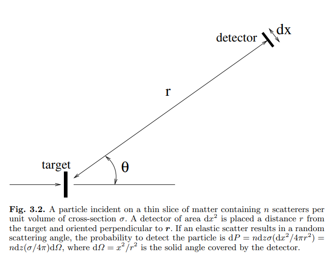
Classically, cross-sections are calculated from the trajectories of particles in force fields. Consider a particle in Fig. 3.9 that passes through a spherically symmetric force field centered on the origin. The particle’s original trajectory is parametrized by the “impact parameter” $b$ which would give the particle’s distance of closest approach to the force center if there were no scattering.
The scattering angle $\theta(b)$ depends on the impact parameter, as in the figure. The relation $\theta(b)$ or $b(\theta)$ can be calculated by integrating the equations of motion with the initial conditions $p_z=p, p_x=p_y=0$. The probability that a particle is scattered into an interval $\mathrm{d} \theta$ about $\theta$ is proportional to the area of the annular region between $b(\theta)$ and $b(\theta+\mathrm{d} \theta)=b+\mathrm{d} b$, i.e. $\mathrm{d} \sigma=2 \pi b \mathrm{~d} b$. The solid angle corresponding to $\mathrm{d} \theta$ is $\mathrm{d} \Omega=2 \pi \sin \theta \mathrm{d} \theta$. The differential elastic scattering cross-section is therefore
$$
\frac{\mathrm{d} \sigma}{\mathrm{d} \Omega}(\theta)=\frac{2 \pi b \mathrm{~d} b}{2 \pi \sin \theta \mathrm{d} \theta}=\left|\frac{b(\theta)}{\sin \theta} \cdot \frac{d b}{d \theta}\right| .
$$
A measurement of $\mathrm{d} \sigma / \mathrm{d} \Omega$ determines the relation $b(\theta)$ which in turn gives information about the potential $V$.

We can apply (3.38) to several simple cases:

Scattering of a point particle on a hard immovable sphere. The angleimpact parameter relation is
$$
b=R \cos \theta / 2,
$$
where $R$ is the radius of the sphere. The cross section is then
$$
\frac{\mathrm{d} \sigma}{\mathrm{d} \Omega}=R^2 / 4 \quad \Rightarrow \quad \sigma=\pi R^2
$$
so the total cross-section is just the geometrical cross section of the sphere. In the case of scattering of two spheres of the same radius, the total scattering cross-section is $\sigma=4 \pi R^2$.

Scattering of a charged particle in a Coulomb potential
$$
V(r)=\frac{Z_1 Z_2 e^2}{4 \pi \epsilon_0 r},
$$
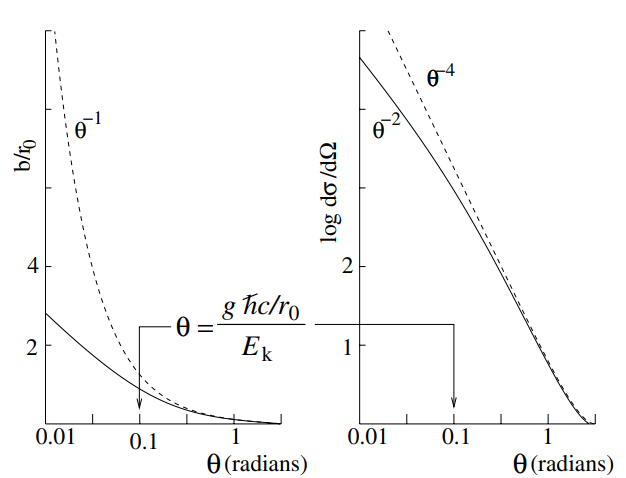
where $Z_1$ is the charge of the scattered particle, and $Z_2$ is the charge of the immobile target particle. This historically important reaction is called “Rutherford scattering” after E. Rutherford who demonstrated the existence of a compact nucleus by studying $\alpha$-particle scattering on gold nuclei. The unbound orbits in the Coulomb potential are hyperbolas so the scattering angle is well-defined in spite of the infinite range of the force. For an incident kinetic energy $E_k=m v^2 / 2$, the angle-impact parameter relation is
$$
b=\frac{Z_1 Z_2 e^2}{8 \pi \epsilon_0 E_k} \cot (\theta / 2) .
$$
The cross-section is then
$$
\frac{d \sigma}{d \Omega}=\left(\frac{Z_1 Z_2 e^2}{16 \pi \epsilon_0 E_k}\right)^2 \frac{1}{\sin ^4 \theta / 2}
$$

物理代写|核物理代写nuclear physics代考|Asymptotic states and their normalization

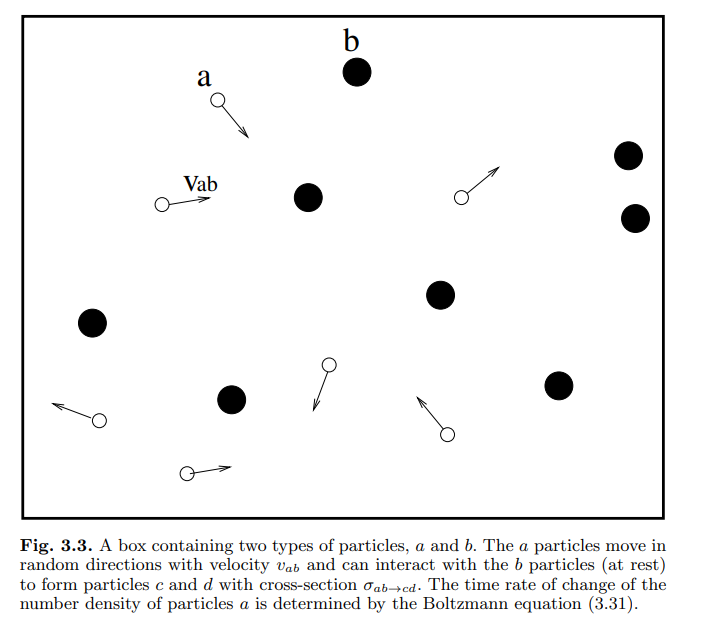
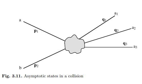
In studying nuclear, or elementary interactions, we are most of the time not interested in a space-time description of phenomena. ${ }^2$ Instead, we study processes in which we prepare initial particles with definite momenta and far away from one another so that they are out of reach of their interactions at an initial time $t_0$ in the “distant past” $t_0 \sim-\infty$. We then study the nature and the momentum distributions of final particles when these are also out of range of the interactions at some later time $t$ in the “distant future” $t \rightarrow+\infty$. (The size of the interaction region is of the order of $1 \mathrm{fm}$, the measuring devices have sizes of the order of a few meters.) Under these assumptions, the initial and final states of the particles under consideration are free particle states. These states are called asymptotic states. The decay of an unstable particle is a particular case. We measure the energy and momenta of final particles in asymptotic states.

By definition, the asymptotic states of particles have definite momenta. Therefore, strictly speaking, they are not physical states, and their wave functions $\mathrm{e}^{\mathrm{i} p x / \hbar}$ are not square integrable. Physically, this means that we are actually interested in wave packets who have a non vanishing but very small extension $\Delta p$ in momentum, i.e. $\Delta p /|p| \ll 1$.

It is possible to work with plane waves, provided one introduces a proper normalization. A limiting procedure, after all calculations are done, allows to get rid of the intermediate regularizing parameters. This is particularly simple in first order Born approximation, which we will present first. The complete manipulation of wave packets is possible but somewhat complicated. However, it gives interesting physical explanations for various specific problems, and we shall discuss it in Sect. 3.3.5.

We will consider that the particles are confined in a (very large but finite) box of volume $L^3$. We will let $L$ tend to infinity at the end of the calculation. Besides its simplicity, this procedure allows to incorporate relativistic kinematics of ingoing and outgoing particles in a simple manner.
In such a box of size $L$, the normalized momentum eigenstates are
$$
\begin{aligned}
|\boldsymbol{p}\rangle \rightarrow \psi_{\boldsymbol{p}}(\boldsymbol{r}) & =L^{-3 / 2} \mathrm{e}^{\mathrm{i} \boldsymbol{p} \cdot \boldsymbol{r} / \hbar} \quad \text { inside the box }, \
\psi_{\boldsymbol{p}}(\boldsymbol{r}) & =0 \quad \text { outside the box } .
\end{aligned}
$$
These wave functions are normalized in the sense that
$$
\int\left|\psi_{\boldsymbol{p}}(\boldsymbol{r})\right|^2 \mathrm{~d}^3 \boldsymbol{r}=1 .
$$

物理代写|核物理代写nuclear physics代考|FYS3500

核物理代写

物理代写|核物理代写nuclear physics代考|Classical cross-sections

经典的横截面是根据粒子在力场中的运动轨迹计算的。考虑图3.9中的一个粒子,它穿过以原点为中心的球对称力场。粒子的原始轨迹由“冲击参数”$b$参数化,该参数将给出粒子在没有散射的情况下最接近力中心的距离。
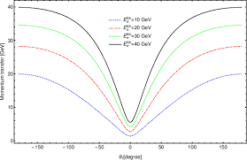
散射角$\theta(b)$取决于冲击参数,如图所示。关系$\theta(b)$或$b(\theta)$可以通过积分运动方程与初始条件$p_z=p, p_x=p_y=0$来计算。粒子散射到$\theta$附近的一个区间$\mathrm{d} \theta$的概率与$b(\theta)$和$b(\theta+\mathrm{d} \theta)=b+\mathrm{d} b$之间的环形区域的面积成正比,即$\mathrm{d} \sigma=2 \pi b \mathrm{~d} b$。$\mathrm{d} \theta$对应的立体角是$\mathrm{d} \Omega=2 \pi \sin \theta \mathrm{d} \theta$。因此,微分弹性散射截面为
$$
\frac{\mathrm{d} \sigma}{\mathrm{d} \Omega}(\theta)=\frac{2 \pi b \mathrm{~d} b}{2 \pi \sin \theta \mathrm{d} \theta}=\left|\frac{b(\theta)}{\sin \theta} \cdot \frac{d b}{d \theta}\right| .
$$
对$\mathrm{d} \sigma / \mathrm{d} \Omega$的测量确定了关系$b(\theta)$,进而给出了关于潜在的$V$的信息。

我们可以将(3.38)应用于几个简单的情况:

点粒子在坚硬的不动球体上的散射。角-冲击参数关系为
$$
b=R \cos \theta / 2,
$$
其中$R$是球体的半径。横截面是
$$
\frac{\mathrm{d} \sigma}{\mathrm{d} \Omega}=R^2 / 4 \quad \Rightarrow \quad \sigma=\pi R^2
$$
所以总横截面就是球面的几何横截面。两个半径相同的球散射时,总散射截面为$\sigma=4 \pi R^2$。

带电粒子在库仑势中的散射
$$
V(r)=\frac{Z_1 Z_2 e^2}{4 \pi \epsilon_0 r},
$$
其中$Z_1$为散射粒子的电荷,$Z_2$为不运动目标粒子的电荷。这个具有重要历史意义的反应被称为“卢瑟福散射”,以E.卢瑟福的名字命名。卢瑟福通过研究$\alpha$ -粒子在金核上的散射,证明了致密核的存在。库仑势中的非束缚轨道是双曲线,所以散射角是明确的,尽管力的范围是无限的。对于入射动能$E_k=m v^2 / 2$,角-冲击参数关系为
$$
b=\frac{Z_1 Z_2 e^2}{8 \pi \epsilon_0 E_k} \cot (\theta / 2) .
$$
横截面是
$$
\frac{d \sigma}{d \Omega}=\left(\frac{Z_1 Z_2 e^2}{16 \pi \epsilon_0 E_k}\right)^2 \frac{1}{\sin ^4 \theta / 2}
$$

物理代写|核物理代写nuclear physics代考|Asymptotic states and their normalization

在研究原子核或基本相互作用时,我们大多数时候对现象的时空描述不感兴趣。${ }^2$相反,我们研究的过程是,我们准备了具有确定动量且彼此远离的初始粒子,使它们在初始时间$t_0$在“遥远的过去”$t_0 \sim-\infty$无法相互作用。然后,我们研究最终粒子的性质和动量分布,当它们也超出相互作用的范围时,在稍后的某个时间$t$在“遥远的未来”$t \rightarrow+\infty$。(相互作用区域的大小为$1 \mathrm{fm}$数量级,测量装置的大小为几米数量级。)在这些假设下,所考虑的粒子的初始和最终状态都是自由粒子状态。这些状态称为渐近状态。不稳定粒子的衰变是一个特例。我们测量了最终粒子在渐近状态下的能量和动量。

根据定义,粒子的渐近状态具有确定的动量。因此,严格地说,它们不是物理状态,它们的波函数$\mathrm{e}^{\mathrm{i} p x / \hbar}$不是平方可积的。在物理上,这意味着我们实际上感兴趣的是具有不消失但动量扩展极小$\Delta p$的波包,即$\Delta p /|p| \ll 1$。

只要引入适当的归一化,就可以处理平面波。在所有的计算完成之后,一个限制程序允许去掉中间的正则化参数。这在一阶玻恩近似中特别简单,我们将首先介绍它。完全操纵波包是可能的,但有些复杂。然而,它为各种具体问题提供了有趣的物理解释,我们将在3.3.5节中讨论它。

我们将考虑粒子被限制在一个(非常大但有限的)体积盒子$L^3$中。我们让$L$在计算结束时趋于无穷。除了它的简单性,这个程序允许以一种简单的方式结合入射和出射粒子的相对论运动学。
在这样一个尺寸为$L$的盒子中,归一化动量本征态是
$$
\begin{aligned}
|\boldsymbol{p}\rangle \rightarrow \psi_{\boldsymbol{p}}(\boldsymbol{r}) & =L^{-3 / 2} \mathrm{e}^{\mathrm{i} \boldsymbol{p} \cdot \boldsymbol{r} / \hbar} \quad \text { inside the box }, \
\psi_{\boldsymbol{p}}(\boldsymbol{r}) & =0 \quad \text { outside the box } .
\end{aligned}
$$
这些波函数在某种意义上是标准化的
$$
\int\left|\psi_{\boldsymbol{p}}(\boldsymbol{r})\right|^2 \mathrm{~d}^3 \boldsymbol{r}=1 .
$$

物理代写|核物理代写nuclear physics代考 请认准statistics-lab™

统计代写请认准statistics-lab™. statistics-lab™为您的留学生涯保驾护航。

金融工程代写

金融工程是使用数学技术来解决金融问题。金融工程使用计算机科学、统计学、经济学和应用数学领域的工具和知识来解决当前的金融问题,以及设计新的和创新的金融产品。

非参数统计代写

非参数统计指的是一种统计方法,其中不假设数据来自于由少数参数决定的规定模型;这种模型的例子包括正态分布模型和线性回归模型。

广义线性模型代考

广义线性模型(GLM)归属统计学领域,是一种应用灵活的线性回归模型。该模型允许因变量的偏差分布有除了正态分布之外的其它分布。

术语 广义线性模型(GLM)通常是指给定连续和/或分类预测因素的连续响应变量的常规线性回归模型。它包括多元线性回归,以及方差分析和方差分析(仅含固定效应)。

有限元方法代写

有限元方法(FEM)是一种流行的方法,用于数值解决工程和数学建模中出现的微分方程。典型的问题领域包括结构分析、传热、流体流动、质量运输和电磁势等传统领域。

有限元是一种通用的数值方法,用于解决两个或三个空间变量的偏微分方程(即一些边界值问题)。为了解决一个问题,有限元将一个大系统细分为更小、更简单的部分,称为有限元。这是通过在空间维度上的特定空间离散化来实现的,它是通过构建对象的网格来实现的:用于求解的数值域,它有有限数量的点。边界值问题的有限元方法表述最终导致一个代数方程组。该方法在域上对未知函数进行逼近。[1] 然后将模拟这些有限元的简单方程组合成一个更大的方程系统,以模拟整个问题。然后,有限元通过变化微积分使相关的误差函数最小化来逼近一个解决方案。

tatistics-lab作为专业的留学生服务机构,多年来已为美国、英国、加拿大、澳洲等留学热门地的学生提供专业的学术服务,包括但不限于Essay代写,Assignment代写,Dissertation代写,Report代写,小组作业代写,Proposal代写,Paper代写,Presentation代写,计算机作业代写,论文修改和润色,网课代做,exam代考等等。写作范围涵盖高中,本科,研究生等海外留学全阶段,辐射金融,经济学,会计学,审计学,管理学等全球99%专业科目。写作团队既有专业英语母语作者,也有海外名校硕博留学生,每位写作老师都拥有过硬的语言能力,专业的学科背景和学术写作经验。我们承诺100%原创,100%专业,100%准时,100%满意。

随机分析代写


随机微积分是数学的一个分支,对随机过程进行操作。它允许为随机过程的积分定义一个关于随机过程的一致的积分理论。这个领域是由日本数学家伊藤清在第二次世界大战期间创建并开始的。

时间序列分析代写

随机过程,是依赖于参数的一组随机变量的全体,参数通常是时间。 随机变量是随机现象的数量表现,其时间序列是一组按照时间发生先后顺序进行排列的数据点序列。通常一组时间序列的时间间隔为一恒定值(如1秒,5分钟,12小时,7天,1年),因此时间序列可以作为离散时间数据进行分析处理。研究时间序列数据的意义在于现实中,往往需要研究某个事物其随时间发展变化的规律。这就需要通过研究该事物过去发展的历史记录,以得到其自身发展的规律。

回归分析代写

多元回归分析渐进(Multiple Regression Analysis Asymptotics)属于计量经济学领域,主要是一种数学上的统计分析方法,可以分析复杂情况下各影响因素的数学关系,在自然科学、社会和经济学等多个领域内应用广泛。

MATLAB代写

MATLAB 是一种用于技术计算的高性能语言。它将计算、可视化和编程集成在一个易于使用的环境中,其中问题和解决方案以熟悉的数学符号表示。典型用途包括:数学和计算算法开发建模、仿真和原型制作数据分析、探索和可视化科学和工程图形应用程序开发,包括图形用户界面构建MATLAB 是一个交互式系统,其基本数据元素是一个不需要维度的数组。这使您可以解决许多技术计算问题,尤其是那些具有矩阵和向量公式的问题,而只需用 C 或 Fortran 等标量非交互式语言编写程序所需的时间的一小部分。MATLAB 名称代表矩阵实验室。MATLAB 最初的编写目的是提供对由 LINPACK 和 EISPACK 项目开发的矩阵软件的轻松访问,这两个项目共同代表了矩阵计算软件的最新技术。MATLAB 经过多年的发展,得到了许多用户的投入。在大学环境中,它是数学、工程和科学入门和高级课程的标准教学工具。在工业领域,MATLAB 是高效研究、开发和分析的首选工具。MATLAB 具有一系列称为工具箱的特定于应用程序的解决方案。对于大多数 MATLAB 用户来说非常重要,工具箱允许您学习应用专业技术。工具箱是 MATLAB 函数(M 文件)的综合集合,可扩展 MATLAB 环境以解决特定类别的问题。可用工具箱的领域包括信号处理、控制系统、神经网络、模糊逻辑、小波、仿真等。

R语言代写问卷设计与分析代写
PYTHON代写回归分析与线性模型代写
MATLAB代写方差分析与试验设计代写
STATA代写机器学习/统计学习代写
SPSS代写计量经济学代写
EVIEWS代写时间序列分析代写
EXCEL代写深度学习代写
SQL代写各种数据建模与可视化代写

物理代写|核物理代写nuclear physics代考|NUC-303

如果你也在 怎样代写核物理Nuclear Physics这个学科遇到相关的难题,请随时右上角联系我们的24/7代写客服。核物理Nuclear Physics在一个世纪的时间里,核物理学发现了数量惊人的应用,并与其他领域建立了联系。

核物理Nuclear Physics在最狭义的意义上,它只涉及质子和中子的束缚系统。然而,从一开始,这种系统的研究之所以取得进展,仅仅是因为人们对其他粒子的理解有所进步:电子、正电子、中微子,以及最终的夸克和胶子。事实上,对于这些“基本粒子”的物理学,我们现在有了比原子核本身更完整的理论。

statistics-lab™ 为您的留学生涯保驾护航 在代写核物理nuclear physics方面已经树立了自己的口碑, 保证靠谱, 高质且原创的统计Statistics代写服务。我们的专家在代写核物理nuclear physics代写方面经验极为丰富,各种代写核物理nuclear physics相关的作业也就用不着说。

物理代写|核物理代写nuclear physics代考|NUC-303

物理代写|核物理代写nuclear physics代考|Inelastic and total cross-sections

In general for a reaction creating $N$ particles
$$
a b \rightarrow x_1 x_2 \ldots x_N
$$
the probability to create the particles $x_i$ in the momentum ranges $\mathrm{d}^3 \boldsymbol{p}i$ centered on the momenta $\boldsymbol{p}_i$ is given by $$ \mathrm{d} P=\frac{\mathrm{d} \sigma}{\mathrm{d}^3 \boldsymbol{p}_1 \ldots \mathrm{d}^3 \boldsymbol{p}_N} n_b \mathrm{~d} z \mathrm{~d}^3 \boldsymbol{p}_1 \ldots \mathrm{d}^3 \boldsymbol{p}_N . $$ The differential cross-section $\mathrm{d} \sigma / \mathrm{d}^3 \boldsymbol{p}_1 \ldots \mathrm{d}^3 \boldsymbol{p}_N$ will be a singular function because only energy-momentum conserving combinations have non-vanishing probabilities. The total probability for the reaction $a b \rightarrow x_1 \ldots x_N$ is $$ \mathrm{d} P{a b \rightarrow x_1 \ldots x_N}=\sigma_{a b \rightarrow x_1 \ldots x_N} n_b \mathrm{~d} z
$$

where the reaction cross-section is
$$
\sigma_{a b \rightarrow x_1 \ldots x_N}=\int \mathrm{d}^3 \boldsymbol{p}1 \ldots \int \mathrm{d}^3 \boldsymbol{p}_N \frac{\mathrm{d} \sigma}{\mathrm{d}^3 \boldsymbol{p}_1 \ldots \mathrm{d}^3 \boldsymbol{p}_N} \mathrm{~d}^3 \boldsymbol{p}_1 \ldots \mathrm{d}^3 \boldsymbol{p}_N . $$ The total probability that “anything” happens to the incident particle as it traverses the target of thickness $\mathrm{d} z$ is just the sum of the probabilities of the individual reactions $$ \mathrm{d} P=\sigma{\text {tot }} n_b \mathrm{~d} z
$$
where the total cross-section is
$$
\sigma_{\mathrm{tot}}=\sum_i \sigma_i
$$

物理代写|核物理代写nuclear physics代考|The uses of cross-sections

Cross-sections enter into an enormous number of calculations in physics. Consider a thin target (Fig. 3.1 ) containing a density $n$ of target particles that is subjected to a flux of beam particles $F$ (particles per unit area per unit time). If particles that interact in the target are considered to be removed from the beam (scattered out of the beam or changed into other types of particles), then the probability for interaction $\mathrm{d} P=\sigma n_{\mathrm{b}} \mathrm{d} z$ implies that the $F$ is reduced by
$$
\mathrm{d} F=-F \sigma n \mathrm{~d} z,
$$
equivalent to the differential equation
$$
\frac{\mathrm{d} F}{\mathrm{~d} z}=-\frac{F}{l},
$$
where the “mean free path” $l$ is
$$
l=\frac{1}{n \sigma} .
$$
For a thick target, (3.25) implies that the flux declines exponentially
$$
F(z)=F(0) \mathrm{e}^{-z / l} .
$$
If the material contains different types of objects $i$ of number density and cross-section $n_i$ and $\sigma_i$, then (3.6) implies that the mean free path is given by
$$
l^{-1}=\sum_i n_i \sigma_i .
$$
The mean lifetime of a particle in the beam is the mean free path divided by the beam velocity $v$
$$
\tau=\frac{l}{v}=\frac{1}{n_{\mathrm{T}} \sigma_{\mathrm{tot}} v} .
$$

The inverse of the mean lifetime is the “reaction rate”
$$
\lambda=n \sigma_{\text {tot }} v .
$$
We will see that quantum-mechanical calculations most naturally yield the reaction rate from which one can derive the cross-section by dividing by $n v$.

物理代写|核物理代写nuclear physics代考|NUC-303

核物理代写

物理代写|核物理代写nuclear physics代考|Inelastic and total cross-sections

一般来说,对于产生$N$粒子的反应
$$
a b \rightarrow x_1 x_2 \ldots x_N
$$
在以动量$\boldsymbol{p}i$为中心的动量范围$\mathrm{d}^3 \boldsymbol{p}i$内产生粒子$x_i$的概率由$$ \mathrm{d} P=\frac{\mathrm{d} \sigma}{\mathrm{d}^3 \boldsymbol{p}_1 \ldots \mathrm{d}^3 \boldsymbol{p}_N} n_b \mathrm{~d} z \mathrm{~d}^3 \boldsymbol{p}_1 \ldots \mathrm{d}^3 \boldsymbol{p}_N . $$给出。微分截面$\mathrm{d} \sigma / \mathrm{d}^3 \boldsymbol{p}_1 \ldots \mathrm{d}^3 \boldsymbol{p}_N$将是一个奇异函数,因为只有能量-动量守恒的组合才具有不消失的概率。反应$a b \rightarrow x_1 \ldots x_N$的总概率是 $$ \mathrm{d} P{a b \rightarrow x_1 \ldots x_N}=\sigma{a b \rightarrow x_1 \ldots x_N} n_b \mathrm{~d} z
$$

反应截面在哪里
$$
\sigma_{a b \rightarrow x_1 \ldots x_N}=\int \mathrm{d}^3 \boldsymbol{p}1 \ldots \int \mathrm{d}^3 \boldsymbol{p}N \frac{\mathrm{d} \sigma}{\mathrm{d}^3 \boldsymbol{p}_1 \ldots \mathrm{d}^3 \boldsymbol{p}_N} \mathrm{~d}^3 \boldsymbol{p}_1 \ldots \mathrm{d}^3 \boldsymbol{p}_N . $$当入射粒子穿过厚度目标时,“任何事情”发生的总概率$\mathrm{d} z$只是单个反应概率的总和$$ \mathrm{d} P=\sigma{\text {tot }} n_b \mathrm{~d} z $$ 总横截面在哪里 $$ \sigma{\mathrm{tot}}=\sum_i \sigma_i
$$

物理代写|核物理代写nuclear physics代考|The uses of cross-sections

在物理学中,横截面涉及到大量的计算。考虑一个薄目标(图3.1),它包含密度为$n$的目标粒子,受到束粒子通量$F$(单位时间内每单位面积上的粒子)的影响。如果在目标中相互作用的粒子被认为从光束中移除(散射出光束或变成其他类型的粒子),那么相互作用的概率$\mathrm{d} P=\sigma n_{\mathrm{b}} \mathrm{d} z$意味着$F$减少了
$$
\mathrm{d} F=-F \sigma n \mathrm{~d} z,
$$
等价于微分方程
$$
\frac{\mathrm{d} F}{\mathrm{~d} z}=-\frac{F}{l},
$$
“平均自由路径”$l$在哪里
$$
l=\frac{1}{n \sigma} .
$$
对于厚目标,(3.25)表示通量呈指数下降
$$
F(z)=F(0) \mathrm{e}^{-z / l} .
$$
如果材料包含不同类型的物体$i$的数量密度和截面$n_i$和$\sigma_i$,则(3.6)意味着平均自由程由
$$
l^{-1}=\sum_i n_i \sigma_i .
$$
粒子在光束中的平均寿命等于平均自由程除以光束速度 $v$
$$
\tau=\frac{l}{v}=\frac{1}{n_{\mathrm{T}} \sigma_{\mathrm{tot}} v} .
$$

平均寿命的倒数是“反应速率”。
$$
\lambda=n \sigma_{\text {tot }} v .
$$
我们将看到,量子力学计算最自然地得出反应速率,我们可以通过除以$n v$得出横截面。

物理代写|核物理代写nuclear physics代考 请认准statistics-lab™

统计代写请认准statistics-lab™. statistics-lab™为您的留学生涯保驾护航。

金融工程代写

金融工程是使用数学技术来解决金融问题。金融工程使用计算机科学、统计学、经济学和应用数学领域的工具和知识来解决当前的金融问题,以及设计新的和创新的金融产品。

非参数统计代写

非参数统计指的是一种统计方法,其中不假设数据来自于由少数参数决定的规定模型;这种模型的例子包括正态分布模型和线性回归模型。

广义线性模型代考

广义线性模型(GLM)归属统计学领域,是一种应用灵活的线性回归模型。该模型允许因变量的偏差分布有除了正态分布之外的其它分布。

术语 广义线性模型(GLM)通常是指给定连续和/或分类预测因素的连续响应变量的常规线性回归模型。它包括多元线性回归,以及方差分析和方差分析(仅含固定效应)。

有限元方法代写

有限元方法(FEM)是一种流行的方法,用于数值解决工程和数学建模中出现的微分方程。典型的问题领域包括结构分析、传热、流体流动、质量运输和电磁势等传统领域。

有限元是一种通用的数值方法,用于解决两个或三个空间变量的偏微分方程(即一些边界值问题)。为了解决一个问题,有限元将一个大系统细分为更小、更简单的部分,称为有限元。这是通过在空间维度上的特定空间离散化来实现的,它是通过构建对象的网格来实现的:用于求解的数值域,它有有限数量的点。边界值问题的有限元方法表述最终导致一个代数方程组。该方法在域上对未知函数进行逼近。[1] 然后将模拟这些有限元的简单方程组合成一个更大的方程系统,以模拟整个问题。然后,有限元通过变化微积分使相关的误差函数最小化来逼近一个解决方案。

tatistics-lab作为专业的留学生服务机构,多年来已为美国、英国、加拿大、澳洲等留学热门地的学生提供专业的学术服务,包括但不限于Essay代写,Assignment代写,Dissertation代写,Report代写,小组作业代写,Proposal代写,Paper代写,Presentation代写,计算机作业代写,论文修改和润色,网课代做,exam代考等等。写作范围涵盖高中,本科,研究生等海外留学全阶段,辐射金融,经济学,会计学,审计学,管理学等全球99%专业科目。写作团队既有专业英语母语作者,也有海外名校硕博留学生,每位写作老师都拥有过硬的语言能力,专业的学科背景和学术写作经验。我们承诺100%原创,100%专业,100%准时,100%满意。

随机分析代写


随机微积分是数学的一个分支,对随机过程进行操作。它允许为随机过程的积分定义一个关于随机过程的一致的积分理论。这个领域是由日本数学家伊藤清在第二次世界大战期间创建并开始的。

时间序列分析代写

随机过程,是依赖于参数的一组随机变量的全体,参数通常是时间。 随机变量是随机现象的数量表现,其时间序列是一组按照时间发生先后顺序进行排列的数据点序列。通常一组时间序列的时间间隔为一恒定值(如1秒,5分钟,12小时,7天,1年),因此时间序列可以作为离散时间数据进行分析处理。研究时间序列数据的意义在于现实中,往往需要研究某个事物其随时间发展变化的规律。这就需要通过研究该事物过去发展的历史记录,以得到其自身发展的规律。

回归分析代写

多元回归分析渐进(Multiple Regression Analysis Asymptotics)属于计量经济学领域,主要是一种数学上的统计分析方法,可以分析复杂情况下各影响因素的数学关系,在自然科学、社会和经济学等多个领域内应用广泛。

MATLAB代写

MATLAB 是一种用于技术计算的高性能语言。它将计算、可视化和编程集成在一个易于使用的环境中,其中问题和解决方案以熟悉的数学符号表示。典型用途包括:数学和计算算法开发建模、仿真和原型制作数据分析、探索和可视化科学和工程图形应用程序开发,包括图形用户界面构建MATLAB 是一个交互式系统,其基本数据元素是一个不需要维度的数组。这使您可以解决许多技术计算问题,尤其是那些具有矩阵和向量公式的问题,而只需用 C 或 Fortran 等标量非交互式语言编写程序所需的时间的一小部分。MATLAB 名称代表矩阵实验室。MATLAB 最初的编写目的是提供对由 LINPACK 和 EISPACK 项目开发的矩阵软件的轻松访问,这两个项目共同代表了矩阵计算软件的最新技术。MATLAB 经过多年的发展,得到了许多用户的投入。在大学环境中,它是数学、工程和科学入门和高级课程的标准教学工具。在工业领域,MATLAB 是高效研究、开发和分析的首选工具。MATLAB 具有一系列称为工具箱的特定于应用程序的解决方案。对于大多数 MATLAB 用户来说非常重要,工具箱允许您学习应用专业技术。工具箱是 MATLAB 函数(M 文件)的综合集合,可扩展 MATLAB 环境以解决特定类别的问题。可用工具箱的领域包括信号处理、控制系统、神经网络、模糊逻辑、小波、仿真等。

R语言代写问卷设计与分析代写
PYTHON代写回归分析与线性模型代写
MATLAB代写方差分析与试验设计代写
STATA代写机器学习/统计学习代写
SPSS代写计量经济学代写
EVIEWS代写时间序列分析代写
EXCEL代写深度学习代写
SQL代写各种数据建模与可视化代写

物理代写|核物理代写nuclear physics代考|SH2302

如果你也在 怎样代写核物理Nuclear Physics这个学科遇到相关的难题,请随时右上角联系我们的24/7代写客服。核物理Nuclear Physics在一个世纪的时间里,核物理学发现了数量惊人的应用,并与其他领域建立了联系。

核物理Nuclear Physics在最狭义的意义上,它只涉及质子和中子的束缚系统。然而,从一开始,这种系统的研究之所以取得进展,仅仅是因为人们对其他粒子的理解有所进步:电子、正电子、中微子,以及最终的夸克和胶子。事实上,对于这些“基本粒子”的物理学,我们现在有了比原子核本身更完整的理论。

statistics-lab™ 为您的留学生涯保驾护航 在代写核物理nuclear physics方面已经树立了自己的口碑, 保证靠谱, 高质且原创的统计Statistics代写服务。我们的专家在代写核物理nuclear physics代写方面经验极为丰富,各种代写核物理nuclear physics相关的作业也就用不着说。

物理代写|核物理代写nuclear physics代考|Two-nucleon system

物理代写|核物理代写nuclear physics代考|The shell model and magic numbers

In atomic physics, the ionization energy $E_I$, i.e. the energy needed to extract an electron from a neutral atom with $Z$ electrons, displays discontinuities around $Z=2,10,18,36,54$ and 86 , i.e. for noble gases. These discontinuities are associated with closed electron shells.

An analogous phenomenon occurs in nuclear physics. There exist many experimental indications showing that atomic nuclei possess a shell-structure and that they can be constructed, like atoms, by filling successive shells of an effective potential well. For example, the nuclear analogs of atomic ionization energies are the “separation energies” $S_{\mathrm{n}}$ and $S_{\mathrm{p}}$ which are necessary in order to extract a neutron or a proton from a nucleus
$$
S_{\mathrm{n}}=B(Z, N)-B(Z, N-1) \quad S_{\mathrm{p}}=B(Z, N)-B(Z-1, N) .
$$
These two quantities present discontinuities at special values of $N$ or $Z$, which are called magic numbers. The most commonly mentioned are:

$$
\begin{array}{lllllll}
2 & 8 & 20 & 28 & 50 & 82 & 126 .
\end{array}
$$
As an example, Fig. 2.7 gives the neutron separation energy of lead isotopes ( $Z=82$ ) as a function of $N$. The discontinuity at the magic number $N=126$ is clearly seen.

The discontinuity in the separation energies is due to the excess binding energy for magic nuclei as compared to that predicted by the semi-empirical Bethe-Weizsäcker mass formula. One can see this in Fig. 2.8 which plots the excess binding energy as a function of $N$ and $Z$. Large positive values of $B / A$ (experimental)- $B / A$ (theory) are observed in the vicinity of the magic numbers for neutrons $N$ as well as for protons $Z$. Figure 2.9 shows the difference as a function of $N$ and $Z$ in the vicinity of the magic numbers 28,50 , 82 and 126 .

物理代写|核物理代写nuclear physics代考|The shell model and the spin-orbit interaction

It is possible to understand the nuclear shell structure within the framework of a modified mean field model. If we assume that the mean potential energy is harmonic, the energy levels are
$$
E_n=(n+3 / 2) \hbar \omega \quad n=n_x+n_y+n_z=0,1,2,3 \ldots,
$$
where $n_{x, y, z}$ are the quantum numbers for the three orthogonal directions and can take on positive semi-definite integers. If we fill up a harmonic well with nucleons, 2 can be placed in the one $n=0$ orbital, i.e. the $\left(n_x, n_y, n_z\right)=$ $(0,0,0)$. We can place 6 in the $n=1$ level because there are 3 orbitals, $(1,0,0),(0,1,0)$ and $(0,0,1)$. The number $N(n)$ are listed in the third row of Table 2.2.

We note that the harmonic potential, like the Coulomb potential, has the peculiarity that the energies depend only on the principal quantum number $n$ and not on the angular momentum quantum number $l$. The angular momentum states, $|n, l, m\rangle$ can be constructed by taking linear combinations of the $\left|n_x, n_y, n_z\right\rangle$ states (Exercise 2.4). The allowed values of $l$ for each $n$ are shown in the second line of Table 2.2.

The magic numbers corresponding to all shells filled below the maximum $n$, as shown on the fourth line of Table 2.2, would then be 2, 8, 20, 40, 70, 112 and 168 in disagreement with observation (2.37). It might be expected that one could find another simple potential that would give the correct numbers. In general one would find that energies would depend on two quantum numbers: the angular momentum quantum number $l$ and a second giving the number of nodes of the radial wavefunction. An example of such a l-splitting is shown in Fig. 2.10. Unfortunately, it turns out that there is no simple potential that gives the correct magic numbers.

The solution to this problem, found in 1949 by M. Göppert Mayer, and by D. Haxel J. Jensen and H. Suess, is to add a spin orbit interaction for each nucleon:
$$
\hat{H}=V_{\mathrm{s}-\mathrm{o}}(r) \hat{\boldsymbol{\ell}} \cdot \hat{\boldsymbol{s}} / \hbar^2
$$

物理代写|核物理代写nuclear physics代考|Two-nucleon system

核物理代写

物理代写|核物理代写nuclear physics代考|The shell model and magic numbers

在原子物理学中,电离能$E_I$,即从具有$Z$电子的中性原子中提取电子所需的能量,在$Z=2,10,18,36,54$和86附近显示不连续,即对于惰性气体。这些不连续与闭合电子壳层有关。

核物理学中也有类似的现象。有许多实验迹象表明原子核具有壳层结构,它们可以像原子一样,通过填充有效势阱的连续壳层来构造。例如,原子电离能的核类似物是“分离能”$S_{\mathrm{n}}$和$S_{\mathrm{p}}$,它们是从原子核中提取中子或质子所必需的
$$
S_{\mathrm{n}}=B(Z, N)-B(Z, N-1) \quad S_{\mathrm{p}}=B(Z, N)-B(Z-1, N) .
$$
这两个量在$N$或$Z$的特殊值处呈现不连续,这些值被称为幻数。最常提到的是:

$$
\begin{array}{lllllll}
2 & 8 & 20 & 28 & 50 & 82 & 126 .
\end{array}
$$
例如,图2.7给出了铅同位素的中子分离能($Z=82$)与$N$的函数关系。在神奇数字$N=126$处的不连续可以清楚地看到。

分离能的不连续性是由于与半经验Bethe-Weizsäcker质量公式预测的相比,魔核的结合能过多。我们可以在图2.8中看到这一点,图2.8将多余的结合能绘制为$N$和$Z$的函数。在中子$N$和质子$Z$的幻数附近,观察到$B / A$(实验)- $B / A$(理论)的大正值。图2.9显示了在神奇数字28、50、82和126附近$N$和$Z$的函数差值。

物理代写|核物理代写nuclear physics代考|The shell model and the spin-orbit interaction

在修正的平均场模型框架内理解核壳结构是可能的。如果我们假设平均势能是调和的,能级是
$$
E_n=(n+3 / 2) \hbar \omega \quad n=n_x+n_y+n_z=0,1,2,3 \ldots,
$$
其中$n_{x, y, z}$为三个正交方向的量子数,可以取正半定整数。如果我们用核子填充一个谐波阱,2可以被放置在一个$n=0$轨道上,即$\left(n_x, n_y, n_z\right)=$$(0,0,0)$。我们可以把6个放在$n=1$层因为有3个轨道,$(1,0,0),(0,1,0)$和$(0,0,1)$。数字$N(n)$列在表2.2的第三行。

我们注意到谐波势,像库仑势一样,具有能量只依赖于主量子数$n$而不依赖于角动量量子数$l$的特性。角动量状态$|n, l, m\rangle$可以通过$\left|n_x, n_y, n_z\right\rangle$状态的线性组合来构造(练习2.4)。表2.2的第二行显示了每个$n$的$l$允许值。

如表2.2第四行所示,填充在最大值$n$以下的所有炮弹对应的幻数将是2,8,20,40,70,112和168,这与观察结果(2.37)不一致。可以预期,人们可以找到另一种简单的势能,可以给出正确的数字。一般来说,人们会发现能量取决于两个量子数:角动量量子数$l$,第二个是径向波函数的节点数。图2.10显示了这种l-分裂的一个例子。不幸的是,事实证明没有简单的势能可以给出正确的神奇数字。

1949年,M. Göppert Mayer、D. Haxel J. Jensen和H. Suess发现了解决这个问题的方法,即为每个核子增加一个自旋轨道相互作用:
$$
\hat{H}=V_{\mathrm{s}-\mathrm{o}}(r) \hat{\boldsymbol{\ell}} \cdot \hat{\boldsymbol{s}} / \hbar^2
$$

物理代写|核物理代写nuclear physics代考 请认准statistics-lab™

统计代写请认准statistics-lab™. statistics-lab™为您的留学生涯保驾护航。

金融工程代写

金融工程是使用数学技术来解决金融问题。金融工程使用计算机科学、统计学、经济学和应用数学领域的工具和知识来解决当前的金融问题,以及设计新的和创新的金融产品。

非参数统计代写

非参数统计指的是一种统计方法,其中不假设数据来自于由少数参数决定的规定模型;这种模型的例子包括正态分布模型和线性回归模型。

广义线性模型代考

广义线性模型(GLM)归属统计学领域,是一种应用灵活的线性回归模型。该模型允许因变量的偏差分布有除了正态分布之外的其它分布。

术语 广义线性模型(GLM)通常是指给定连续和/或分类预测因素的连续响应变量的常规线性回归模型。它包括多元线性回归,以及方差分析和方差分析(仅含固定效应)。

有限元方法代写

有限元方法(FEM)是一种流行的方法,用于数值解决工程和数学建模中出现的微分方程。典型的问题领域包括结构分析、传热、流体流动、质量运输和电磁势等传统领域。

有限元是一种通用的数值方法,用于解决两个或三个空间变量的偏微分方程(即一些边界值问题)。为了解决一个问题,有限元将一个大系统细分为更小、更简单的部分,称为有限元。这是通过在空间维度上的特定空间离散化来实现的,它是通过构建对象的网格来实现的:用于求解的数值域,它有有限数量的点。边界值问题的有限元方法表述最终导致一个代数方程组。该方法在域上对未知函数进行逼近。[1] 然后将模拟这些有限元的简单方程组合成一个更大的方程系统,以模拟整个问题。然后,有限元通过变化微积分使相关的误差函数最小化来逼近一个解决方案。

tatistics-lab作为专业的留学生服务机构,多年来已为美国、英国、加拿大、澳洲等留学热门地的学生提供专业的学术服务,包括但不限于Essay代写,Assignment代写,Dissertation代写,Report代写,小组作业代写,Proposal代写,Paper代写,Presentation代写,计算机作业代写,论文修改和润色,网课代做,exam代考等等。写作范围涵盖高中,本科,研究生等海外留学全阶段,辐射金融,经济学,会计学,审计学,管理学等全球99%专业科目。写作团队既有专业英语母语作者,也有海外名校硕博留学生,每位写作老师都拥有过硬的语言能力,专业的学科背景和学术写作经验。我们承诺100%原创,100%专业,100%准时,100%满意。

随机分析代写


随机微积分是数学的一个分支,对随机过程进行操作。它允许为随机过程的积分定义一个关于随机过程的一致的积分理论。这个领域是由日本数学家伊藤清在第二次世界大战期间创建并开始的。

时间序列分析代写

随机过程,是依赖于参数的一组随机变量的全体,参数通常是时间。 随机变量是随机现象的数量表现,其时间序列是一组按照时间发生先后顺序进行排列的数据点序列。通常一组时间序列的时间间隔为一恒定值(如1秒,5分钟,12小时,7天,1年),因此时间序列可以作为离散时间数据进行分析处理。研究时间序列数据的意义在于现实中,往往需要研究某个事物其随时间发展变化的规律。这就需要通过研究该事物过去发展的历史记录,以得到其自身发展的规律。

回归分析代写

多元回归分析渐进(Multiple Regression Analysis Asymptotics)属于计量经济学领域,主要是一种数学上的统计分析方法,可以分析复杂情况下各影响因素的数学关系,在自然科学、社会和经济学等多个领域内应用广泛。

MATLAB代写

MATLAB 是一种用于技术计算的高性能语言。它将计算、可视化和编程集成在一个易于使用的环境中,其中问题和解决方案以熟悉的数学符号表示。典型用途包括:数学和计算算法开发建模、仿真和原型制作数据分析、探索和可视化科学和工程图形应用程序开发,包括图形用户界面构建MATLAB 是一个交互式系统,其基本数据元素是一个不需要维度的数组。这使您可以解决许多技术计算问题,尤其是那些具有矩阵和向量公式的问题,而只需用 C 或 Fortran 等标量非交互式语言编写程序所需的时间的一小部分。MATLAB 名称代表矩阵实验室。MATLAB 最初的编写目的是提供对由 LINPACK 和 EISPACK 项目开发的矩阵软件的轻松访问,这两个项目共同代表了矩阵计算软件的最新技术。MATLAB 经过多年的发展,得到了许多用户的投入。在大学环境中,它是数学、工程和科学入门和高级课程的标准教学工具。在工业领域,MATLAB 是高效研究、开发和分析的首选工具。MATLAB 具有一系列称为工具箱的特定于应用程序的解决方案。对于大多数 MATLAB 用户来说非常重要,工具箱允许您学习应用专业技术。工具箱是 MATLAB 函数(M 文件)的综合集合,可扩展 MATLAB 环境以解决特定类别的问题。可用工具箱的领域包括信号处理、控制系统、神经网络、模糊逻辑、小波、仿真等。

R语言代写问卷设计与分析代写
PYTHON代写回归分析与线性模型代写
MATLAB代写方差分析与试验设计代写
STATA代写机器学习/统计学习代写
SPSS代写计量经济学代写
EVIEWS代写时间序列分析代写
EXCEL代写深度学习代写
SQL代写各种数据建模与可视化代写

物理代写|核物理代写nuclear physics代考|Two-nucleon system

如果你也在 怎样代写核物理nuclear physics这个学科遇到相关的难题,请随时右上角联系我们的24/7代写客服。

核物理学是研究原子核及其成分和相互作用的物理学领域,此外还研究其他形式的核物质。核物理学不应与原子物理学相混淆,后者研究原子的整体,包括其电子。

statistics-lab™ 为您的留学生涯保驾护航 在代写核物理nuclear physics方面已经树立了自己的口碑, 保证靠谱, 高质且原创的统计Statistics代写服务。我们的专家在代写核物理nuclear physics代写方面经验极为丰富,各种代写核物理nuclear physics相关的作业也就用不着说。

物理代写|核物理代写nuclear physics代考|Two-nucleon system

物理代写|核物理代写nuclear physics代考|Two-nucleon system

The isospin states of a two-nucleon system are constructed in the same manner as the states of two spin $1 / 2$ particles.
The total isospin $T$ of the system corresponds to:
$$
T=1 \text { or } T=0
$$
and the four corresponding eigenstates are :
$$
\begin{gathered}
\left|T=1, T_3\right\rangle:\left{\begin{array}{l}
\left|T=1, T_3=1\right\rangle=|\mathrm{pp}\rangle \
\left|T=1, T_3=0\right\rangle=(|\mathrm{pn}\rangle+|\mathrm{np}\rangle) / \sqrt{2} \
\left|T=1, T_3=-1\right\rangle=|\mathrm{nn}\rangle
\end{array}\right. \
\left|T=0, T_3=0\right\rangle: \quad|0,0\rangle=(|\mathrm{pn}\rangle-|\mathrm{np}\rangle) / \sqrt{2} .
\end{gathered}
$$
We recall that, just as for spin, the three states $|T=1, M\rangle$ are collectively called the isospin triplet. They are symmetric under the exchange of the components of the two particles along $T_3$. The state $|T=0,0\rangle$ is called the isospin singlet state. It is antisymmetric in that exchange. The triplet state transforms as a vector under rotations in isospin space. The singlet state is invariant under those rotations.

物理代写|核物理代写nuclear physics代考|Origin of isospin symmetry; n-p mass difference

The near-equality of the proton and neutron masses is a necessary ingredient for isospin symmetry to appear. This symmetry can be understood quite naturally in the context of the quark model where nucleons are states of three quarks. The proton is a (uud) bound state of two u quarks of charge $2 / 3$ and one d quark of charge $-1 / 3$. The neutron is a (udd) bound state, with two d quarks and one u quark.

Quarks interact according to the laws of “quantum chromodynamics” or QCD. In this theory, forces are universal in the sense that they make strictly no distinction between types, or flavors, of quarks involved. The only difference between the $\mathrm{u}$ and $\mathrm{d}$ quarks are their masses or charges and we can expect that the proton and neutron masses differ because of the differing quark masses and/or from electromagnetic effects.

It is tempting to suppose that isospin is an exact symmetry of strong nuclear interactions and that electromagnetism is a calculable, and comparatively small, correction. In that framework, it would be natural to assume that, in the absence of electromagnetic forces, the proton and neutron masses should be equal and that their difference originates from calculable electromagnetic effects.

We know experimentally that the proton and neutron are extended objects; as we shall see in Chap. 3 , the proton has a radius of the order $r \sim 1 \mathrm{fm}$. To first approximation, the neutron does not have an electrostatic energy. The electrostatic energy of the proton is of the order of
$$
E_{e s} \simeq \frac{q_e^2}{4 \pi \varepsilon_0 r} \simeq 1.3 \mathrm{MeV},
$$
which is indeed very close to the observed value neutron-proton mass difference, except for the wrong sign!

物理代写|核物理代写nuclear physics代考|Two-nucleon system

核物理代写

物理代写|核物理代写nuclear physics代考|Two-nucleon system

双核子系统的同位旋态以与两个自旋$1 / 2$粒子的状态相同的方式构造。
体系的总同位旋$T$对应于:
$$
T=1 \text { or } T=0
$$
对应的四个特征态为:
$$
\begin{gathered}
\left|T=1, T_3\right\rangle:\left{\begin{array}{l}
\left|T=1, T_3=1\right\rangle=|\mathrm{pp}\rangle \
\left|T=1, T_3=0\right\rangle=(|\mathrm{pn}\rangle+|\mathrm{np}\rangle) / \sqrt{2} \
\left|T=1, T_3=-1\right\rangle=|\mathrm{nn}\rangle
\end{array}\right. \
\left|T=0, T_3=0\right\rangle: \quad|0,0\rangle=(|\mathrm{pn}\rangle-|\mathrm{np}\rangle) / \sqrt{2} .
\end{gathered}
$$
我们记得,就像自旋一样,这三个态$|T=1, M\rangle$统称为同位旋三重态。它们在两个粒子沿$T_3$方向的分量交换下是对称的。状态$|T=0,0\rangle$被称为同位旋单重态。在这个交换中它是反对称的。三重态在同位旋空间中作为矢量在旋转下变换。单重态在这些旋转下是不变的。

物理代写|核物理代写nuclear physics代考|Origin of isospin symmetry; n-p mass difference

质子和中子的质量接近相等是同位旋对称出现的必要条件。在夸克模型的背景下,这种对称性可以很自然地理解,在夸克模型中,核子是三个夸克的状态。质子是两个带电荷的u夸克$2 / 3$和一个带电荷的d夸克$-1 / 3$的(ud)束缚态。中子是一个(udd)束缚态,有两个d夸克和一个u夸克。

夸克根据“量子色动力学”(QCD)定律相互作用。在这个理论中,力是普遍的,因为它们对所涉及的夸克的类型或味道没有严格的区分。$\mathrm{u}$和$\mathrm{d}$夸克之间的唯一区别是它们的质量或电荷,我们可以预期质子和中子的质量不同,因为不同的夸克质量和/或电磁效应。

人们很容易认为同位旋是强核相互作用的一种精确对称,而电磁是一种可计算的、相对较小的修正。在这个框架下,很自然地可以假设,在没有电磁力的情况下,质子和中子的质量应该是相等的,它们的差异源于可计算的电磁效应。

我们从实验上知道质子和中子是延展的物体;我们将在第三章看到,质子的半径为$r \sim 1 \mathrm{fm}$数量级。根据第一个近似,中子不具有静电能。质子的静电能约为
$$
E_{e s} \simeq \frac{q_e^2}{4 \pi \varepsilon_0 r} \simeq 1.3 \mathrm{MeV},
$$
这确实非常接近观测值中子-质子质量差,除了错误的符号!

物理代写|核物理代写nuclear physics代考 请认准statistics-lab™

统计代写请认准statistics-lab™. statistics-lab™为您的留学生涯保驾护航。

金融工程代写

金融工程是使用数学技术来解决金融问题。金融工程使用计算机科学、统计学、经济学和应用数学领域的工具和知识来解决当前的金融问题,以及设计新的和创新的金融产品。

非参数统计代写

非参数统计指的是一种统计方法,其中不假设数据来自于由少数参数决定的规定模型;这种模型的例子包括正态分布模型和线性回归模型。

广义线性模型代考

广义线性模型(GLM)归属统计学领域,是一种应用灵活的线性回归模型。该模型允许因变量的偏差分布有除了正态分布之外的其它分布。

术语 广义线性模型(GLM)通常是指给定连续和/或分类预测因素的连续响应变量的常规线性回归模型。它包括多元线性回归,以及方差分析和方差分析(仅含固定效应)。

有限元方法代写

有限元方法(FEM)是一种流行的方法,用于数值解决工程和数学建模中出现的微分方程。典型的问题领域包括结构分析、传热、流体流动、质量运输和电磁势等传统领域。

有限元是一种通用的数值方法,用于解决两个或三个空间变量的偏微分方程(即一些边界值问题)。为了解决一个问题,有限元将一个大系统细分为更小、更简单的部分,称为有限元。这是通过在空间维度上的特定空间离散化来实现的,它是通过构建对象的网格来实现的:用于求解的数值域,它有有限数量的点。边界值问题的有限元方法表述最终导致一个代数方程组。该方法在域上对未知函数进行逼近。[1] 然后将模拟这些有限元的简单方程组合成一个更大的方程系统,以模拟整个问题。然后,有限元通过变化微积分使相关的误差函数最小化来逼近一个解决方案。

tatistics-lab作为专业的留学生服务机构,多年来已为美国、英国、加拿大、澳洲等留学热门地的学生提供专业的学术服务,包括但不限于Essay代写,Assignment代写,Dissertation代写,Report代写,小组作业代写,Proposal代写,Paper代写,Presentation代写,计算机作业代写,论文修改和润色,网课代做,exam代考等等。写作范围涵盖高中,本科,研究生等海外留学全阶段,辐射金融,经济学,会计学,审计学,管理学等全球99%专业科目。写作团队既有专业英语母语作者,也有海外名校硕博留学生,每位写作老师都拥有过硬的语言能力,专业的学科背景和学术写作经验。我们承诺100%原创,100%专业,100%准时,100%满意。

随机分析代写


随机微积分是数学的一个分支,对随机过程进行操作。它允许为随机过程的积分定义一个关于随机过程的一致的积分理论。这个领域是由日本数学家伊藤清在第二次世界大战期间创建并开始的。

时间序列分析代写

随机过程,是依赖于参数的一组随机变量的全体,参数通常是时间。 随机变量是随机现象的数量表现,其时间序列是一组按照时间发生先后顺序进行排列的数据点序列。通常一组时间序列的时间间隔为一恒定值(如1秒,5分钟,12小时,7天,1年),因此时间序列可以作为离散时间数据进行分析处理。研究时间序列数据的意义在于现实中,往往需要研究某个事物其随时间发展变化的规律。这就需要通过研究该事物过去发展的历史记录,以得到其自身发展的规律。

回归分析代写

多元回归分析渐进(Multiple Regression Analysis Asymptotics)属于计量经济学领域,主要是一种数学上的统计分析方法,可以分析复杂情况下各影响因素的数学关系,在自然科学、社会和经济学等多个领域内应用广泛。

MATLAB代写

MATLAB 是一种用于技术计算的高性能语言。它将计算、可视化和编程集成在一个易于使用的环境中,其中问题和解决方案以熟悉的数学符号表示。典型用途包括:数学和计算算法开发建模、仿真和原型制作数据分析、探索和可视化科学和工程图形应用程序开发,包括图形用户界面构建MATLAB 是一个交互式系统,其基本数据元素是一个不需要维度的数组。这使您可以解决许多技术计算问题,尤其是那些具有矩阵和向量公式的问题,而只需用 C 或 Fortran 等标量非交互式语言编写程序所需的时间的一小部分。MATLAB 名称代表矩阵实验室。MATLAB 最初的编写目的是提供对由 LINPACK 和 EISPACK 项目开发的矩阵软件的轻松访问,这两个项目共同代表了矩阵计算软件的最新技术。MATLAB 经过多年的发展,得到了许多用户的投入。在大学环境中,它是数学、工程和科学入门和高级课程的标准教学工具。在工业领域,MATLAB 是高效研究、开发和分析的首选工具。MATLAB 具有一系列称为工具箱的特定于应用程序的解决方案。对于大多数 MATLAB 用户来说非常重要,工具箱允许您学习应用专业技术。工具箱是 MATLAB 函数(M 文件)的综合集合,可扩展 MATLAB 环境以解决特定类别的问题。可用工具箱的领域包括信号处理、控制系统、神经网络、模糊逻辑、小波、仿真等。

R语言代写问卷设计与分析代写
PYTHON代写回归分析与线性模型代写
MATLAB代写方差分析与试验设计代写
STATA代写机器学习/统计学习代写
SPSS代写计量经济学代写
EVIEWS代写时间序列分析代写
EXCEL代写深度学习代写
SQL代写各种数据建模与可视化代写

物理代写|核物理代写nuclear physics代考|Energy-momentum conservation

如果你也在 怎样代写核物理nuclear physics这个学科遇到相关的难题,请随时右上角联系我们的24/7代写客服。

核物理学是研究原子核及其成分和相互作用的物理学领域,此外还研究其他形式的核物质。核物理学不应与原子物理学相混淆,后者研究原子的整体,包括其电子。

statistics-lab™ 为您的留学生涯保驾护航 在代写核物理nuclear physics方面已经树立了自己的口碑, 保证靠谱, 高质且原创的统计Statistics代写服务。我们的专家在代写核物理nuclear physics代写方面经验极为丰富,各种代写核物理nuclear physics相关的作业也就用不着说。

物理代写|核物理代写nuclear physics代考|Energy-momentum conservation

物理代写|核物理代写nuclear physics代考|Energy-momentum conservation

By far the most important conservation law is that for Energy-momentum. For example, in nuclear $\beta$-decay
$$
(A, Z) \rightarrow(A, Z+1) \mathrm{e}^{-} \overline{\mathrm{v}}{\mathrm{e}} $$ we require $$ E{A, Z}=E_{A, Z+1}+E_{\mathrm{e}}+E_{\bar{v}{\mathrm{e}}}, $$ and $$ \boldsymbol{p}{A, Z}=\boldsymbol{p}{A, Z+1}+\boldsymbol{p}{\mathrm{e}}+\boldsymbol{p}{\overline{\mathrm{v}}{\mathrm{e}}}
$$
These two laws are only constraints. As discussed in later chapters, the way that momentum and energy are distributed between the decay products depends on the details of the interaction responsible for the reaction.

When one applies energy-momentum conservation, it is of course necessary to take into account the masses of initial and final particles by using the relativistic expression for the energy
$$
E=\left(p^2 c^2+m^2 c^4\right)^{1 / 2}
$$
for a free particle of mass $m$. The square root in this formula often makes calculations very difficult. However, in nuclear physics, nuclei and nucleons are usually non-relativistic, $v=p c^2 / E \ll c$, and one can use the non-relativistic approximation :
$$
E=\sqrt{p^2 c^2+m^2 c^4} \simeq m c^2+p^2 / 2 m
$$
i.e. the energy is the sum of the rest energy $m c^2$ and the non-relativistic kinetic energy $p^2 / 2 m$. On the other hand, photons and neutrinos are relativistic:
$$
E=\sqrt{p^2 c^2+m^2 c^4} \simeq p c+m^2 c^4 / 2 p c,
$$
where the mass term $m^2 c^4 / 2 p c$ can usually be neglected for neutrinos and always for the massless photon $E=p c$.

物理代写|核物理代写nuclear physics代考|Angular momentum and parity (non)conservation

Angular momentum conservations plays a different role than that of energymomentum conservation. The latter can by verified to a useful precision in individual events where the energies and momenta of final-state particles can be compared with those of the initial-state particles. This is because there is a relatively well-defined correspondence between momentum wavefunctions (plane waves) and the classical tracks of particles that are actually observed, i.e. a plane wave of wave vector $\boldsymbol{k}$ and angular frequency $\omega$ generates a detector response that appears to be due to a classical particle of momentum $\hbar \boldsymbol{k}$ and energy $E=\hbar \omega$.

On the other hand, the wavefunctions corresponding to a definite angular momentum, correspond to certain angular dependence of the function about the origin. This information is lost when an individual track going in a particular direction is measured. It can be recovered only by observing many events and reconstructing the angular distribution.

The same consideration applies to parity which gives the behavior of a wavefunction under reversal of all coordinates. Its conservation can only be verified in the distribution of tracks. As it turns out, parity is not in fact conserved in the weak interactions, as we will see in Chap. 4.

物理代写|核物理代写nuclear physics代考|Energy-momentum conservation

核物理代写

物理代写|核物理代写nuclear physics代考|Energy-momentum conservation

到目前为止,最重要的守恒定律是能量动量守恒定律。例如,在核$\beta$衰变中
$$
(A, Z) \rightarrow(A, Z+1) \mathrm{e}^{-} \overline{\mathrm{v}}{\mathrm{e}} $$我们需要$$ E{A, Z}=E_{A, Z+1}+E_{\mathrm{e}}+E_{\bar{v}{\mathrm{e}}}, $$和$$ \boldsymbol{p}{A, Z}=\boldsymbol{p}{A, Z+1}+\boldsymbol{p}{\mathrm{e}}+\boldsymbol{p}{\overline{\mathrm{v}}{\mathrm{e}}}
$$
这两条定律只是约束。正如后面章节所讨论的,动量和能量在衰变产物之间分布的方式取决于引起反应的相互作用的细节。

当应用能量-动量守恒时,当然有必要通过使用能量的相对论表达式来考虑初始粒子和最终粒子的质量
$$
E=\left(p^2 c^2+m^2 c^4\right)^{1 / 2}
$$
对于一个有质量的自由粒子$m$。这个公式中的平方根常常使计算变得非常困难。然而,在核物理学中,原子核和核子通常是非相对论性的,$v=p c^2 / E \ll c$,我们可以使用非相对论性近似:
$$
E=\sqrt{p^2 c^2+m^2 c^4} \simeq m c^2+p^2 / 2 m
$$
也就是说,能量是静止能量$m c^2$和非相对论动能$p^2 / 2 m$之和。另一方面,光子和中微子是相对论性的:
$$
E=\sqrt{p^2 c^2+m^2 c^4} \simeq p c+m^2 c^4 / 2 p c,
$$
质量项$m^2 c^4 / 2 p c$对于中微子通常可以忽略对于无质量光子$E=p c$也是如此。

物理代写|核物理代写nuclear physics代考|Angular momentum and parity (non)conservation

角动量守恒与能量动量守恒起着不同的作用。后者可以在个别事件中得到有用的精确验证,其中末态粒子的能量和动量可以与初始态粒子的能量和动量进行比较。这是因为动量波函数(平面波)与实际观察到的粒子的经典轨迹之间存在相对明确的对应关系,即波矢量$\boldsymbol{k}$和角频率$\omega$的平面波产生的探测器响应似乎是由于动量$\hbar \boldsymbol{k}$和能量$E=\hbar \omega$的经典粒子引起的。

另一方面,波函数对应于一个确定的角动量,对应于函数关于原点的角依赖性。当测量特定方向上的单个轨道时,这些信息就丢失了。只有通过观测多个事件,重建角度分布,才能恢复。

同样的考虑也适用于奇偶性,它给出了波函数在所有坐标反转下的行为。它的保存只能在轨道的分布中得到验证。事实证明,宇称在弱相互作用中实际上并不守恒,我们将在第四章看到这一点。

物理代写|核物理代写nuclear physics代考 请认准statistics-lab™

统计代写请认准statistics-lab™. statistics-lab™为您的留学生涯保驾护航。

金融工程代写

金融工程是使用数学技术来解决金融问题。金融工程使用计算机科学、统计学、经济学和应用数学领域的工具和知识来解决当前的金融问题,以及设计新的和创新的金融产品。

非参数统计代写

非参数统计指的是一种统计方法,其中不假设数据来自于由少数参数决定的规定模型;这种模型的例子包括正态分布模型和线性回归模型。

广义线性模型代考

广义线性模型(GLM)归属统计学领域,是一种应用灵活的线性回归模型。该模型允许因变量的偏差分布有除了正态分布之外的其它分布。

术语 广义线性模型(GLM)通常是指给定连续和/或分类预测因素的连续响应变量的常规线性回归模型。它包括多元线性回归,以及方差分析和方差分析(仅含固定效应)。

有限元方法代写

有限元方法(FEM)是一种流行的方法,用于数值解决工程和数学建模中出现的微分方程。典型的问题领域包括结构分析、传热、流体流动、质量运输和电磁势等传统领域。

有限元是一种通用的数值方法,用于解决两个或三个空间变量的偏微分方程(即一些边界值问题)。为了解决一个问题,有限元将一个大系统细分为更小、更简单的部分,称为有限元。这是通过在空间维度上的特定空间离散化来实现的,它是通过构建对象的网格来实现的:用于求解的数值域,它有有限数量的点。边界值问题的有限元方法表述最终导致一个代数方程组。该方法在域上对未知函数进行逼近。[1] 然后将模拟这些有限元的简单方程组合成一个更大的方程系统,以模拟整个问题。然后,有限元通过变化微积分使相关的误差函数最小化来逼近一个解决方案。

tatistics-lab作为专业的留学生服务机构,多年来已为美国、英国、加拿大、澳洲等留学热门地的学生提供专业的学术服务,包括但不限于Essay代写,Assignment代写,Dissertation代写,Report代写,小组作业代写,Proposal代写,Paper代写,Presentation代写,计算机作业代写,论文修改和润色,网课代做,exam代考等等。写作范围涵盖高中,本科,研究生等海外留学全阶段,辐射金融,经济学,会计学,审计学,管理学等全球99%专业科目。写作团队既有专业英语母语作者,也有海外名校硕博留学生,每位写作老师都拥有过硬的语言能力,专业的学科背景和学术写作经验。我们承诺100%原创,100%专业,100%准时,100%满意。

随机分析代写


随机微积分是数学的一个分支,对随机过程进行操作。它允许为随机过程的积分定义一个关于随机过程的一致的积分理论。这个领域是由日本数学家伊藤清在第二次世界大战期间创建并开始的。

时间序列分析代写

随机过程,是依赖于参数的一组随机变量的全体,参数通常是时间。 随机变量是随机现象的数量表现,其时间序列是一组按照时间发生先后顺序进行排列的数据点序列。通常一组时间序列的时间间隔为一恒定值(如1秒,5分钟,12小时,7天,1年),因此时间序列可以作为离散时间数据进行分析处理。研究时间序列数据的意义在于现实中,往往需要研究某个事物其随时间发展变化的规律。这就需要通过研究该事物过去发展的历史记录,以得到其自身发展的规律。

回归分析代写

多元回归分析渐进(Multiple Regression Analysis Asymptotics)属于计量经济学领域,主要是一种数学上的统计分析方法,可以分析复杂情况下各影响因素的数学关系,在自然科学、社会和经济学等多个领域内应用广泛。

MATLAB代写

MATLAB 是一种用于技术计算的高性能语言。它将计算、可视化和编程集成在一个易于使用的环境中,其中问题和解决方案以熟悉的数学符号表示。典型用途包括:数学和计算算法开发建模、仿真和原型制作数据分析、探索和可视化科学和工程图形应用程序开发,包括图形用户界面构建MATLAB 是一个交互式系统,其基本数据元素是一个不需要维度的数组。这使您可以解决许多技术计算问题,尤其是那些具有矩阵和向量公式的问题,而只需用 C 或 Fortran 等标量非交互式语言编写程序所需的时间的一小部分。MATLAB 名称代表矩阵实验室。MATLAB 最初的编写目的是提供对由 LINPACK 和 EISPACK 项目开发的矩阵软件的轻松访问,这两个项目共同代表了矩阵计算软件的最新技术。MATLAB 经过多年的发展,得到了许多用户的投入。在大学环境中,它是数学、工程和科学入门和高级课程的标准教学工具。在工业领域,MATLAB 是高效研究、开发和分析的首选工具。MATLAB 具有一系列称为工具箱的特定于应用程序的解决方案。对于大多数 MATLAB 用户来说非常重要,工具箱允许您学习应用专业技术。工具箱是 MATLAB 函数(M 文件)的综合集合,可扩展 MATLAB 环境以解决特定类别的问题。可用工具箱的领域包括信号处理、控制系统、神经网络、模糊逻辑、小波、仿真等。

R语言代写问卷设计与分析代写
PYTHON代写回归分析与线性模型代写
MATLAB代写方差分析与试验设计代写
STATA代写机器学习/统计学习代写
SPSS代写计量经济学代写
EVIEWS代写时间序列分析代写
EXCEL代写深度学习代写
SQL代写各种数据建模与可视化代写

物理代写|核物理代写nuclear physics代考|Mass units and measurements

如果你也在 怎样代写核物理nuclear physics这个学科遇到相关的难题,请随时右上角联系我们的24/7代写客服。

核物理学是研究原子核及其成分和相互作用的物理学领域,此外还研究其他形式的核物质。核物理学不应与原子物理学相混淆,后者研究原子的整体,包括其电子。

statistics-lab™ 为您的留学生涯保驾护航 在代写核物理nuclear physics方面已经树立了自己的口碑, 保证靠谱, 高质且原创的统计Statistics代写服务。我们的专家在代写核物理nuclear physics代写方面经验极为丰富,各种代写核物理nuclear physics相关的作业也就用不着说。

物理代写|核物理代写nuclear physics代考|Mass units and measurements

物理代写|核物理代写nuclear physics代考|Mass units and measurements

The binding energies of the previous section were defined (1.12) in terms of nuclear and nucleon masses. Most masses are now measured with a precision of $\sim 10^{-8}$ so binding energies can be determined with a precision of $\sim 10^{-6}$. This is sufficiently precise to test the most sophisticated nuclear models that can predict binding energies at the level of $10^{-4}$ at best.

Three units are commonly used to described nuclear masses: the atomic mass unit (u), the kilogram ( $\mathrm{kg})$, and the electron-volt (eV) for rest energies, $m c^2$. In this book we generally use the energy unit eV since energy is a more general concept than mass and is hence more practical in calculations involving nuclear reactions.

It is worth taking some time to explain clearly the differences between the three systems. The atomic mass unit is a purely microscopic unit in that the mass of $\mathrm{a}^{12} \mathrm{C}$ atom is defined to be $12 \mathrm{u}$ :
$$
m\left({ }^{12} \mathrm{C} \text { atom }\right) \equiv 12 \mathrm{u}
$$
The masses of other atoms, nuclei or particles are found by measuring ratios of masses. On the other hand, the kilogram is a macroscopic unit, being defined as the mass of a certain platinum-iridium bar housed in Sèvres, a suburb of Paris. Atomic masses on the kilogram scale can be found by assembling a known (macroscopic) number of atoms and comparing the mass of the assembly with that of the bar. Finally, the eV is a hybrid microscopic-macroscopic unit, being defined as the kinetic energy of an electron after being accelerated from rest through a potential difference of $1 \mathrm{~V}$.

Some important and very accurately known masses are listed in Table 1.2.

物理代写|核物理代写nuclear physics代考|Quantum states of nuclei

While $(A, Z)$ is sufficient to denote a nuclear species, a given $(A, Z)$ will generally have a large number of quantum states corresponding to different wavefunctions of the constituent nucleons. This is, of course, entirely analogous to the situation in atomic physics where an atom of atomic number $Z$ will have a lowest energy state (ground state) and a spectrum of excited states. Some typical nuclear spectra are shown in Fig. 1.6.

In both atomic and nuclear physics, transitions from the higher energy states to the ground state occurs rapidly. The details of this process will be discussed in Sect. 4.2. For an isolated nucleus the transition occurs with the emission of photons to conserve energy. The photons emitted during the decay of excited nuclear states are called $\gamma$-rays. A excited nucleus surrounded by atomic electrons can also transfer its energy to an electron which is subsequently ejected. This process is called internal conversion and the ejected electrons are called conversion electrons. The energy spectrum of $\gamma$-rays and conversion electrons can be used to derive the spectrum of nuclear excited states.

Lifetimes of nuclear excited states are typically in the range $10^{-15}-$ $14^{-10} \mathrm{~s}$. Because of the short lifetimes, with few exceptions only nuclei in the ground state are present on Earth. The rare excited states with lifetimes greater than, say, $1 \mathrm{~s}$ are called isomers. An extreme example is the first exited state of ${ }^{180} \mathrm{Ta}$ which has a lifetime of $10^{15} \mathrm{yr}$ whereas the ground state $\beta$-decays with a lifetime of $8 \mathrm{hr}$. All ${ }^{180} \mathrm{Ta}$ present on Earth is therefore in the excited state.
Isomeric states are generally specified by placing a $m$ after $A$, i.e.
${ }^{180 \mathrm{~m}} \mathrm{Ta}$.

物理代写|核物理代写nuclear physics代考|Mass units and measurements

核物理代写

物理代写|核物理代写nuclear physics代考|Mass units and measurements

上一节的结合能是根据核质量和核子质量定义的(1.12)。现在测量大多数质量的精度为$\sim 10^{-8}$,因此确定结合能的精度为$\sim 10^{-6}$。这足够精确,可以测试最复杂的核模型,这些模型最多可以预测$10^{-4}$级别的结合能。

通常有三个单位用于描述核质量:原子质量单位(u)、千克($\mathrm{kg})$)和静止能量的电子伏特(eV) $m c^2$。在这本书中,我们通常使用能量单位eV,因为能量是一个比质量更一般的概念,因此在涉及核反应的计算中更实用。

花点时间来解释清楚这三种体系之间的区别是值得的。原子质量单位是一个纯粹的微观单位,因为$\mathrm{a}^{12} \mathrm{C}$原子的质量定义为$12 \mathrm{u}$:
$$
m\left({ }^{12} \mathrm{C} \text { atom }\right) \equiv 12 \mathrm{u}
$$
其他原子、原子核或粒子的质量是通过测量质量比来确定的。另一方面,千克是一个宏观单位,被定义为位于巴黎郊区s的某块铂铱棒的质量。千克级的原子质量可以通过组装已知(宏观)数量的原子并将组装的质量与棒材的质量进行比较来计算。最后,eV是微观-宏观的混合单位,定义为电子从静止加速后,通过$1 \mathrm{~V}$的电位差得到的动能。

物理代写|核物理代写nuclear physics代考|Quantum states of nuclei

虽然$(A, Z)$足以表示核种,但给定的$(A, Z)$通常具有与组成核子的不同波函数相对应的大量量子态。当然,这完全类似于原子物理学中的情况,原子序数$Z$的原子将具有最低能量状态(基态)和激发态谱。一些典型的核谱如图1.6所示。

在原子物理和核物理中,从高能态到基态的跃迁发生得很快。这个过程的细节将在4.2节中讨论。对于孤立的原子核来说,跃迁是随着光子的发射而发生的,以保存能量。在激发态衰变过程中发射的光子称为$\gamma$射线。被原子电子包围的激发态原子核也能将其能量传递给随后被射出的电子。这个过程被称为内部转换,射出的电子被称为转换电子。利用$\gamma$射线和转换电子的能谱可以推导出核激发态的能谱。

核激发态的寿命通常在$10^{-15}-$$14^{-10} \mathrm{~s}$范围内。由于寿命短,地球上除了少数例外只有基态的原子核存在。寿命大于$1 \mathrm{~s}$的稀有激发态称为同分异构体。一个极端的例子是${ }^{180} \mathrm{Ta}$的第一激发态,其寿命为$10^{15} \mathrm{yr}$,而基态$\beta$ -衰变的寿命为$8 \mathrm{hr}$。因此,地球上的所有${ }^{180} \mathrm{Ta}$都处于激发态。
同分异构体状态通常通过在$A$后面加上$m$来指定。
${ }^{180 \mathrm{~m}} \mathrm{Ta}$。

物理代写|核物理代写nuclear physics代考 请认准statistics-lab™

统计代写请认准statistics-lab™. statistics-lab™为您的留学生涯保驾护航。

金融工程代写

金融工程是使用数学技术来解决金融问题。金融工程使用计算机科学、统计学、经济学和应用数学领域的工具和知识来解决当前的金融问题,以及设计新的和创新的金融产品。

非参数统计代写

非参数统计指的是一种统计方法,其中不假设数据来自于由少数参数决定的规定模型;这种模型的例子包括正态分布模型和线性回归模型。

广义线性模型代考

广义线性模型(GLM)归属统计学领域,是一种应用灵活的线性回归模型。该模型允许因变量的偏差分布有除了正态分布之外的其它分布。

术语 广义线性模型(GLM)通常是指给定连续和/或分类预测因素的连续响应变量的常规线性回归模型。它包括多元线性回归,以及方差分析和方差分析(仅含固定效应)。

有限元方法代写

有限元方法(FEM)是一种流行的方法,用于数值解决工程和数学建模中出现的微分方程。典型的问题领域包括结构分析、传热、流体流动、质量运输和电磁势等传统领域。

有限元是一种通用的数值方法,用于解决两个或三个空间变量的偏微分方程(即一些边界值问题)。为了解决一个问题,有限元将一个大系统细分为更小、更简单的部分,称为有限元。这是通过在空间维度上的特定空间离散化来实现的,它是通过构建对象的网格来实现的:用于求解的数值域,它有有限数量的点。边界值问题的有限元方法表述最终导致一个代数方程组。该方法在域上对未知函数进行逼近。[1] 然后将模拟这些有限元的简单方程组合成一个更大的方程系统,以模拟整个问题。然后,有限元通过变化微积分使相关的误差函数最小化来逼近一个解决方案。

tatistics-lab作为专业的留学生服务机构,多年来已为美国、英国、加拿大、澳洲等留学热门地的学生提供专业的学术服务,包括但不限于Essay代写,Assignment代写,Dissertation代写,Report代写,小组作业代写,Proposal代写,Paper代写,Presentation代写,计算机作业代写,论文修改和润色,网课代做,exam代考等等。写作范围涵盖高中,本科,研究生等海外留学全阶段,辐射金融,经济学,会计学,审计学,管理学等全球99%专业科目。写作团队既有专业英语母语作者,也有海外名校硕博留学生,每位写作老师都拥有过硬的语言能力,专业的学科背景和学术写作经验。我们承诺100%原创,100%专业,100%准时,100%满意。

随机分析代写


随机微积分是数学的一个分支,对随机过程进行操作。它允许为随机过程的积分定义一个关于随机过程的一致的积分理论。这个领域是由日本数学家伊藤清在第二次世界大战期间创建并开始的。

时间序列分析代写

随机过程,是依赖于参数的一组随机变量的全体,参数通常是时间。 随机变量是随机现象的数量表现,其时间序列是一组按照时间发生先后顺序进行排列的数据点序列。通常一组时间序列的时间间隔为一恒定值(如1秒,5分钟,12小时,7天,1年),因此时间序列可以作为离散时间数据进行分析处理。研究时间序列数据的意义在于现实中,往往需要研究某个事物其随时间发展变化的规律。这就需要通过研究该事物过去发展的历史记录,以得到其自身发展的规律。

回归分析代写

多元回归分析渐进(Multiple Regression Analysis Asymptotics)属于计量经济学领域,主要是一种数学上的统计分析方法,可以分析复杂情况下各影响因素的数学关系,在自然科学、社会和经济学等多个领域内应用广泛。

MATLAB代写

MATLAB 是一种用于技术计算的高性能语言。它将计算、可视化和编程集成在一个易于使用的环境中,其中问题和解决方案以熟悉的数学符号表示。典型用途包括:数学和计算算法开发建模、仿真和原型制作数据分析、探索和可视化科学和工程图形应用程序开发,包括图形用户界面构建MATLAB 是一个交互式系统,其基本数据元素是一个不需要维度的数组。这使您可以解决许多技术计算问题,尤其是那些具有矩阵和向量公式的问题,而只需用 C 或 Fortran 等标量非交互式语言编写程序所需的时间的一小部分。MATLAB 名称代表矩阵实验室。MATLAB 最初的编写目的是提供对由 LINPACK 和 EISPACK 项目开发的矩阵软件的轻松访问,这两个项目共同代表了矩阵计算软件的最新技术。MATLAB 经过多年的发展,得到了许多用户的投入。在大学环境中,它是数学、工程和科学入门和高级课程的标准教学工具。在工业领域,MATLAB 是高效研究、开发和分析的首选工具。MATLAB 具有一系列称为工具箱的特定于应用程序的解决方案。对于大多数 MATLAB 用户来说非常重要,工具箱允许您学习应用专业技术。工具箱是 MATLAB 函数(M 文件)的综合集合,可扩展 MATLAB 环境以解决特定类别的问题。可用工具箱的领域包括信号处理、控制系统、神经网络、模糊逻辑、小波、仿真等。

R语言代写问卷设计与分析代写
PYTHON代写回归分析与线性模型代写
MATLAB代写方差分析与试验设计代写
STATA代写机器学习/统计学习代写
SPSS代写计量经济学代写
EVIEWS代写时间序列分析代写
EXCEL代写深度学习代写
SQL代写各种数据建模与可视化代写

物理代写|核物理代写nuclear physics代考|ERICE2022

如果你也在 怎样代写核物理nuclear physics这个学科遇到相关的难题,请随时右上角联系我们的24/7代写客服。

核物理学是研究原子核及其成分和相互作用的物理学领域,此外还研究其他形式的核物质。核物理学不应与原子物理学相混淆,后者研究原子的整体,包括其电子。

statistics-lab™ 为您的留学生涯保驾护航 在代写核物理nuclear physics方面已经树立了自己的口碑, 保证靠谱, 高质且原创的统计Statistics代写服务。我们的专家在代写核物理nuclear physics代写方面经验极为丰富,各种代写核物理nuclear physics相关的作业也就用不着说。

我们提供的核物理nuclear physics及其相关学科的代写,服务范围广, 其中包括但不限于:

  • Statistical Inference 统计推断
  • Statistical Computing 统计计算
  • Advanced Probability Theory 高等概率论
  • Advanced Mathematical Statistics 高等数理统计学
  • (Generalized) Linear Models 广义线性模型
  • Statistical Machine Learning 统计机器学习
  • Longitudinal Data Analysis 纵向数据分析
  • Foundations of Data Science 数据科学基础
物理代写|核物理代写nuclear physics代考|ERICE2022

物理代写|核物理代写nuclear physics代考|Feynman Diagrams

We therefore have a relativistic expression for the scattering amplitude of two particles, $a$ and $b$ (masses $m_a$ and $m_b$ ) with initial energies and momenta $\left(E_1, \boldsymbol{p}_1\right),\left(E_2, \boldsymbol{p}_2\right)$ and final energies and momenta $\left(E_3, \boldsymbol{p}_3\right),\left(E_4, \boldsymbol{p}_4\right)$. The amplitude can be represented diagrammatically as shown in Fig.16.1, which represents the scattering of two (different) particles due to the exchange of a gauge boson (force carrier) with mass $M$. This is known as a “Feynman diagram” (or “Feynman graph”) [89]. The amplitude for the process is obtained by applying a set of “Feynman rules” for each vertex, where particles interact with each other, and each internal line (the propagation of the virtual off mass-shell particle). The full set of Feynman rules takes into account the spins of the external and internal particles, which requires a detailed study of Quantum Field Theory.

Some of the Feynman rules for constructing the contribution to the amplitude from a Feynman diagram are:

  • Include a (dimensionless) factor of $-g_a / \sqrt{\hbar c}$ at each vertex involving particle interacting with an exchanged gauge boson, with coupling constant $g_a$.
  • Conserve energy and momentum at each vertex.
  • Include a propagator factor:
    $$
    \Delta(E, \boldsymbol{p}, M)=-\frac{1}{\left(E^2-p^2 c^2-M^2 c^4\right)},
    $$
    for each internal particle of mass $M$ carrying energy $E$ and momentum $\boldsymbol{p}$.
  • Include a factor of $(\hbar c)^{3 / 2} / \sqrt{V}$ for each outgoing particle.
    For the process described by the Feynman diagram of Fig. 16.1, conservation of energy and momentum at each vertex leads to
    $$
    \begin{gathered}
    E_q=\left(E_3-E_1\right)=\left(E_2-E_4\right) \
    \boldsymbol{q}=\boldsymbol{p}_3-\boldsymbol{p}_1=\boldsymbol{p}_2-\boldsymbol{p}_4
    \end{gathered}
    $$

物理代写|核物理代写nuclear physics代考|Multiple Feynman Graphs

The internal particles must be attached to the external particles in all possible ways. Figure 16.1 represents the scattering of two different particles in which the internal gauge boson couples the initial particle with energy and momentum $\left(E_1, \boldsymbol{p}1\right)$ to the final particle with energy $\left(E_3, \boldsymbol{p}_3\right)$ at one end, and the other initial particle with energy and momentum $\left(E_2, \boldsymbol{p}_2\right)$ to the other final particle with energy $\left(E_4, p_4\right)$ at the other end. This diagram also appears in Fig. 16.2a. In the case of identical particles, it is also possible for the gauge boson to couple the initial particle with energy and momentum $\left(E_1, \boldsymbol{p}_1\right)$ to the final particle with energy $\left(E_4, \boldsymbol{p}_4\right)$ at one end, and to couple the initial particle with energy and momentum $\left(E_2, \boldsymbol{p}_2\right)$ to the final particle with energy $\left(E_3, p_3\right)$ at the other as shown in Fig. 16.2b. For diagram $(b)$, the internal particle carries energy and momentum $\left(E{q^{\prime}}, \boldsymbol{q}^{\prime}\right)$, given by
$$
\begin{aligned}
E_{q^{\prime}} & =E_1-E_4=E_3-E_2 \
\boldsymbol{q}^{\prime} & =\boldsymbol{p}1-\boldsymbol{p}_4=\boldsymbol{p}_3-\boldsymbol{p}_2 . \end{aligned} $$ The scattering amplitude is the sum of the contributions from the two graphs. When the square modulus of the amplitude ${ }^2$ is taken, in order to calculate the cross section, there is a quantum interference term, namely the product of the contribution from the one Feynman diagram with the complex conjugate of the contribution from the other Feynman diagram. If the contributions from the two diagrams in Fig. 16.2 are $\mathcal{A}{(a)}$ and $\mathcal{A}{(b)}$, respectively, then the square modulus of the amplitude is given by $$ |\mathcal{A}|^2=\left|\mathcal{A}{(a)}\right|^2+\left|\mathcal{A}{(b)}\right|^2+\mathcal{A}{(a)}^* \mathcal{A}{(b)}+\mathcal{A}{(b)}^* \mathcal{A}_{(a)} .
$$

物理代写|核物理代写nuclear physics代考|ERICE2022

核物理代写

物理代写|核物理代写nuclear physics代考|Feynman Diagrams

因此,我们有两个粒子散射振幅的相对论表达式, $a$ 和 $b$ (群众 $m_a$ 和 $m_b$ ) 具有初始能量和动量 $\left(E_1, \boldsymbol{p}_1\right),\left(E_2, \boldsymbol{p}_2\right)$ 最后的能量和动量 $\left(E_3, \boldsymbol{p}_3\right),\left(E_4, \boldsymbol{p}_4\right)$. 振幅可以用图解表示,如图 16.1 所示, 它表示由于规范玻色子 (力载体) 与质量的交换而导致的两个 (不同) 粒子的散射 $M$. 这被称为“费曼图” (或”费曼图”) [89]。该过程的振幅是通过对每个顶点应用一组“费曼规则”获得的,其中粒子彼此相互作 用,以及每条内部线(虚拟脱离质量壳粒子的传播)。全套费鄤规则考虑了外部和内部粒子的自旋,这 需要详细研究量子场论。
从费曼图构造对振幅的贡献的一些费曼规则是:

  • 包括一个 (无量纲) 因素 $-g_a / \sqrt{\hbar c}$ 在涉及粒子与交换规范玻色子相互作用的每个顶点,具有耦合 常数 $g_a$.
  • 在每个顶点保存能量和动量。
  • 包括传播因子:
    $$
    \Delta(E, \boldsymbol{p}, M)=-\frac{1}{\left(E^2-p^2 c^2-M^2 c^4\right)}
    $$
    对于每个内部质量粒子 $M$ 承载能量 $E$ 和势头 $\boldsymbol{p}$.
  • 包括一个因素 $(\hbar c)^{3 / 2} / \sqrt{V}$ 对于每个传出粒子。 对于图 16.1 的费曼图所描述的过程,每个顶点的能量和动量守恒导致
    $$
    E_q=\left(E_3-E_1\right)=\left(E_2-E_4\right) \boldsymbol{q}=\boldsymbol{p}_3-\boldsymbol{p}_1=\boldsymbol{p}_2-\boldsymbol{p}_4
    $$

物理代写|核物理代写nuclear physics代考|Multiple Feynman Graphs

内部粒子必须以所有可能的方式附着在外部粒子上。图 16.1 表示两个不同粒子的散射,其中内部规范玻 色子将初始粒子与能量和动量耦合 $\left(E_1, \boldsymbol{p} 1\right)$ 到最后一个有能量的粒子 $\left(E_3, \boldsymbol{p}3\right)$ 在一端,另一个具有能 量和动量的初始粒子 $\left(E_2, \boldsymbol{p}_2\right)$ 到另一个有能量的最终粒子 $\left(E_4, p_4\right)$ 在另一端。该图也出现在图 16.2a 中。在相同粒子的情况下,规范玻色子也可能将初始粒子与能量和动量耦合 $\left(E_1, \boldsymbol{p}_1\right)$ 到最后一个有能量 的粒子 $\left(E_4, \boldsymbol{p}_4\right)$ 在一端,并将初始粒子与能量和动量耦合 $\left(E_2, \boldsymbol{p}_2\right)$ 到最后一个有能量的粒子 $\left(E_3, p_3\right)$ 在另一个如图 16.2b 所示。对于图表 $(b)$ ,内部粒子携带能量和动量 $\left(E q^{\prime}, \boldsymbol{q}^{\prime}\right)$ ,由 $$ E{q^{\prime}}=E_1-E_4=E_3-E_2 \boldsymbol{q}^{\prime} \quad=\boldsymbol{p} 1-\boldsymbol{p}4=\boldsymbol{p}_3-\boldsymbol{p}_2 . $$ 散射幅度是两个图贡献的总和。当振幅的平方模 ${ }^2$ 被取,为了计算横截面,有一个量子干涉项,即一个费 曼图的贡献与另一个费曼图的贡献的复共轭的乘积。如果图 16.2 中两个图的贡献是 $\mathcal{A}(a)$ 和 $\mathcal{A}(b)$, 则振 幅的平方模由下式给出 $$ |\mathcal{A}|^2=|\mathcal{A}(a)|^2+|\mathcal{A}(b)|^2+\mathcal{A}(a)^* \mathcal{A}(b)+\mathcal{A}(b)^* \mathcal{A}{(a)} .
$$

物理代写|核物理代写nuclear physics代考 请认准statistics-lab™

统计代写请认准statistics-lab™. statistics-lab™为您的留学生涯保驾护航。

金融工程代写

金融工程是使用数学技术来解决金融问题。金融工程使用计算机科学、统计学、经济学和应用数学领域的工具和知识来解决当前的金融问题,以及设计新的和创新的金融产品。

非参数统计代写

非参数统计指的是一种统计方法,其中不假设数据来自于由少数参数决定的规定模型;这种模型的例子包括正态分布模型和线性回归模型。

广义线性模型代考

广义线性模型(GLM)归属统计学领域,是一种应用灵活的线性回归模型。该模型允许因变量的偏差分布有除了正态分布之外的其它分布。

术语 广义线性模型(GLM)通常是指给定连续和/或分类预测因素的连续响应变量的常规线性回归模型。它包括多元线性回归,以及方差分析和方差分析(仅含固定效应)。

有限元方法代写

有限元方法(FEM)是一种流行的方法,用于数值解决工程和数学建模中出现的微分方程。典型的问题领域包括结构分析、传热、流体流动、质量运输和电磁势等传统领域。

有限元是一种通用的数值方法,用于解决两个或三个空间变量的偏微分方程(即一些边界值问题)。为了解决一个问题,有限元将一个大系统细分为更小、更简单的部分,称为有限元。这是通过在空间维度上的特定空间离散化来实现的,它是通过构建对象的网格来实现的:用于求解的数值域,它有有限数量的点。边界值问题的有限元方法表述最终导致一个代数方程组。该方法在域上对未知函数进行逼近。[1] 然后将模拟这些有限元的简单方程组合成一个更大的方程系统,以模拟整个问题。然后,有限元通过变化微积分使相关的误差函数最小化来逼近一个解决方案。

tatistics-lab作为专业的留学生服务机构,多年来已为美国、英国、加拿大、澳洲等留学热门地的学生提供专业的学术服务,包括但不限于Essay代写,Assignment代写,Dissertation代写,Report代写,小组作业代写,Proposal代写,Paper代写,Presentation代写,计算机作业代写,论文修改和润色,网课代做,exam代考等等。写作范围涵盖高中,本科,研究生等海外留学全阶段,辐射金融,经济学,会计学,审计学,管理学等全球99%专业科目。写作团队既有专业英语母语作者,也有海外名校硕博留学生,每位写作老师都拥有过硬的语言能力,专业的学科背景和学术写作经验。我们承诺100%原创,100%专业,100%准时,100%满意。

随机分析代写


随机微积分是数学的一个分支,对随机过程进行操作。它允许为随机过程的积分定义一个关于随机过程的一致的积分理论。这个领域是由日本数学家伊藤清在第二次世界大战期间创建并开始的。

时间序列分析代写

随机过程,是依赖于参数的一组随机变量的全体,参数通常是时间。 随机变量是随机现象的数量表现,其时间序列是一组按照时间发生先后顺序进行排列的数据点序列。通常一组时间序列的时间间隔为一恒定值(如1秒,5分钟,12小时,7天,1年),因此时间序列可以作为离散时间数据进行分析处理。研究时间序列数据的意义在于现实中,往往需要研究某个事物其随时间发展变化的规律。这就需要通过研究该事物过去发展的历史记录,以得到其自身发展的规律。

回归分析代写

多元回归分析渐进(Multiple Regression Analysis Asymptotics)属于计量经济学领域,主要是一种数学上的统计分析方法,可以分析复杂情况下各影响因素的数学关系,在自然科学、社会和经济学等多个领域内应用广泛。

MATLAB代写

MATLAB 是一种用于技术计算的高性能语言。它将计算、可视化和编程集成在一个易于使用的环境中,其中问题和解决方案以熟悉的数学符号表示。典型用途包括:数学和计算算法开发建模、仿真和原型制作数据分析、探索和可视化科学和工程图形应用程序开发,包括图形用户界面构建MATLAB 是一个交互式系统,其基本数据元素是一个不需要维度的数组。这使您可以解决许多技术计算问题,尤其是那些具有矩阵和向量公式的问题,而只需用 C 或 Fortran 等标量非交互式语言编写程序所需的时间的一小部分。MATLAB 名称代表矩阵实验室。MATLAB 最初的编写目的是提供对由 LINPACK 和 EISPACK 项目开发的矩阵软件的轻松访问,这两个项目共同代表了矩阵计算软件的最新技术。MATLAB 经过多年的发展,得到了许多用户的投入。在大学环境中,它是数学、工程和科学入门和高级课程的标准教学工具。在工业领域,MATLAB 是高效研究、开发和分析的首选工具。MATLAB 具有一系列称为工具箱的特定于应用程序的解决方案。对于大多数 MATLAB 用户来说非常重要,工具箱允许您学习应用专业技术。工具箱是 MATLAB 函数(M 文件)的综合集合,可扩展 MATLAB 环境以解决特定类别的问题。可用工具箱的领域包括信号处理、控制系统、神经网络、模糊逻辑、小波、仿真等。

R语言代写问卷设计与分析代写
PYTHON代写回归分析与线性模型代写
MATLAB代写方差分析与试验设计代写
STATA代写机器学习/统计学习代写
SPSS代写计量经济学代写
EVIEWS代写时间序列分析代写
EXCEL代写深度学习代写
SQL代写各种数据建模与可视化代写

物理代写|核物理代写nuclear physics代考|MATR316

如果你也在 怎样代写核物理nuclear physics这个学科遇到相关的难题,请随时右上角联系我们的24/7代写客服。

核物理学是研究原子核及其成分和相互作用的物理学领域,此外还研究其他形式的核物质。核物理学不应与原子物理学相混淆,后者研究原子的整体,包括其电子。

statistics-lab™ 为您的留学生涯保驾护航 在代写核物理nuclear physics方面已经树立了自己的口碑, 保证靠谱, 高质且原创的统计Statistics代写服务。我们的专家在代写核物理nuclear physics代写方面经验极为丰富,各种代写核物理nuclear physics相关的作业也就用不着说。

我们提供的核物理nuclear physics及其相关学科的代写,服务范围广, 其中包括但不限于:

  • Statistical Inference 统计推断
  • Statistical Computing 统计计算
  • Advanced Probability Theory 高等概率论
  • Advanced Mathematical Statistics 高等数理统计学
  • (Generalized) Linear Models 广义线性模型
  • Statistical Machine Learning 统计机器学习
  • Longitudinal Data Analysis 纵向数据分析
  • Foundations of Data Science 数据科学基础
物理代写|核物理代写nuclear physics代考|MATR316

物理代写|核物理代写nuclear physics代考|Relativistic Approach to Interactions

In Particle Physics, we are studying the interactions between sub-microscopic particles that are usually moving with velocities close to the speed of light. We therefore need a synthesis of Quantum Physics and Special Relativity in order to describe these interactions.

There are two fundamental differences between non-relativistic and relativistic Quantum Physics:

  1. The Schroedinger equation describes a particle moving under a certain potential. In Special Relativity there is no such thing as a potential since this would imply an instantaneous action at the distance.
  2. Since energy can be converted into mass and vice versa, particle number in a relativistic scattering event is not conserved – particles can annihilate with each other and new particles can be created. A Schroedinger wavefunction, which is normalized such that the probability of finding a particle somewhere in space is always unity, is clearly an unsuitable tool for describing such processes.

We therefore seek to modify the non-relativistic concept of potential in such a way that relativistic invariance is satisfied.

The potential due to a force, whose force carrier (gauge boson) has mass $M$, is given by the Yukawa potential [105]:
$$
V(r)=\frac{g^2}{4 \pi r} e^{-M c r / \hbar}
$$
where $g^2$ is a measure of the strength of the interaction that generates this potential. The quantum matrix element, $\mathcal{A}(q)$, of this potential between an initial state of a free particle with momentum $\boldsymbol{p}$ and a final state of a free particle with momentum $p+q$ (confined to a box of volume $V$ ) is $$
\mathcal{A}(\boldsymbol{q})=\frac{1}{V} \int d^3 \boldsymbol{r} \frac{g^2}{4 \pi r} \exp \left{\frac{(i \boldsymbol{q} \cdot \boldsymbol{r}-M c \boldsymbol{r})}{\hbar}\right}=\frac{1}{V} \frac{g^2 \hbar^2}{\left(\boldsymbol{q}^2+M^2 c^2\right)}
$$
This is not a relativistically invariant expression as the momentum transfer, $\boldsymbol{q}$, changes under a Lorentz transformation. The expression of the RHS of (16.2) can be modified to cast it into a relativistically invariant quantity, by altering it to
$$
\mathcal{A}\left(E_q, \boldsymbol{q}\right)=\frac{1}{V}(g \hbar c)^2 \Delta\left(E_q, \boldsymbol{q}, M\right)
$$
where
$$
\Delta\left(E_q, \boldsymbol{q}, M\right)=-\frac{1}{\left(E_q^2-\boldsymbol{q}^2 c^2-M^2 c^4\right)}
$$

物理代写|核物理代写nuclear physics代考|Relativistic Momentum Transfer

In Chap. 13 we introduced the relativistically invariant variable $s$, which in the CM frame is equal to the total energy of the incoming (or outgoing) particles. In the same way, the relativistically invariant variable $t$ is used to generalize the momentum transfer. This quantity $[101]$ is defined as
$$
t=E_q^2-q^2 c^2
$$
In terms of $t$, the propagator is
$$
\Delta(t, M)=-\frac{1}{t-M^2 c^4}
$$
In the $\mathrm{CM}$ frame, $t$ is very simply related to the scattering angle, $\theta_{\mathrm{CM}}$, between the directions of the initial and final particle momentum. $\boldsymbol{p}1$ and $\boldsymbol{p}_3$. $$ t=-2 p{\mathrm{CM}}^2 c^2\left(1-\cos \theta_{\mathrm{CM}}\right)=-\left(2 p_{\mathrm{CM}} c \sin \left(\frac{\theta_{\mathrm{CM}}}{2}\right)\right)^2,
$$
where $p_{\mathrm{CM}}$ is the magnitude of the momentum of the particles in the $\mathrm{CM}$ frame. In this frame, $\sqrt{-t} / c$ is the momentum transfer (see (2.7)). The (negative) value of $t$ ranges from $-4 p_{\mathrm{CM}}^2 c^2$ to zero.

The magnitude, $p_{\mathrm{CM}}$, of the momentum of the incident particles in the CM frame can be related to $s$ using the relation between energy and momentum
$$
\sqrt{s}=E_1+E_2=\sqrt{p_{\mathrm{CM}}^2 c^2+m_a^2 c^4}+\sqrt{p_{\mathrm{CM}}^2 c^2+m_b^2 c^4},
$$
where $m_a$ and $m_b$ are the masses of the two incoming particles. After some algebra we can write $p_{\mathrm{CM}}$ in a manifestly Lorentz invariant form, as a function of $s, m_a$ and $m_b$.

物理代写|核物理代写nuclear physics代考|MATR316

核物理代写

物理代写|核物理代写nuclear physics代考|Relativistic Approach to Interactions

在粒子物理学中,我们正在研究通常以接近光速的速度运动的亚微观粒子之间的相互作用。因此,我们 需要综合量子物理学和狭义相对论来描述这些相互作用。
非相对论和相对论量子物理学之间有两个根本区别:

  1. 薛定谔方程描述了在一定电势下运动的粒子。在狭义相对论中,没有势这样的东西,因为这意味着 远处的瞬时作用。
  2. 由于能量可以转化为质量,反之亦然,相对论散射事件中的粒子数不守恒一一粒子可以相互湮灭并 产生新粒子。薛定谔波函数被归一化,使得在空间某处找到粒子的概率始终为 1,显然不适合描述 此类过程的工具。
    因此,我们寻求以满足相对论不变性的方式修改势的非相对论概念。
    由于力的势能,其力载体(规范玻色子)具有质量 $M$ ,由汤川势 [105] 给出:
    $$
    V(r)=\frac{g^2}{4 \pi r} e^{-M c r / \hbar}
    $$
    在哪里 $g^2$ 是衡量产生这种潜力的相互作用的强度。量子矩阵元, $\mathcal{A}(q)$ ,具有动量的自由粒子的初始状态 之间的这种势能 $p$ 和具有动量的自由粒子的最终状态 $p+q$ (限于一盅体积 $V$ ) 是
    这不是动量传递的相对论不变表达式, $\boldsymbol{q}$, 在洛伦兹变换下发生变化。可以修改 (16.2) 的 RHS 表达式以 将其转换为相对论不变的量,方法是将其更改为
    $$
    \mathcal{A}\left(E_q, \boldsymbol{q}\right)=\frac{1}{V}(g \hbar c)^2 \Delta\left(E_q, \boldsymbol{q}, M\right)
    $$
    在哪里
    $$
    \Delta\left(E_q, \boldsymbol{q}, M\right)=-\frac{1}{\left(E_q^2-\boldsymbol{q}^2 c^2-M^2 c^4\right)}
    $$

物理代写|核物理代写nuclear physics代考|Relativistic Momentum Transfer

在第一章 13 我们引入了相对论不变变量 $s$ ,在 $\mathrm{CM}$ 框架中等于入射 (或出射) 粒子的总能量。同理,相 对论不变变量 $t$ 用于概括动量传递。这个数量 $[101]$ 定义为
$$
t=E_q^2-q^2 c^2
$$
按照 $t$ ,传播者是
$$
\Delta(t, M)=-\frac{1}{t-M^2 c^4}
$$
在里面CM框架, $t$ 与散射角非常简单地相关, $\theta_{\mathrm{CM}}$ ,在初始和最终粒子动量的方向之间。 $\boldsymbol{p} 1$ 和 $\boldsymbol{p}3$. $$ t=-2 p \mathrm{CM}^2 c^2\left(1-\cos \theta{\mathrm{CM}}\right)=-\left(2 p_{\mathrm{CM}} c \sin \left(\frac{\theta_{\mathrm{CM}}}{2}\right)\right)^2
$$
在哪里 $p_{\mathrm{CM}}$ 是粒子动量的大小 $\mathrm{CM}$ 框架。在这个框架中, $\sqrt{-t} / c$ 是动量传递(见 (2.7) )。的 (负) 值 $t$ 范围从 $-4 p_{\mathrm{CM}}^2 c^2$ 归零。
幅度, $p_{\mathrm{CM}}$ ,在 $\mathrm{CM}$ 框架中入射粒子的动量可以与 $s$ 利用能量和动量之间的关系
$$
\sqrt{s}=E_1+E_2=\sqrt{p_{\mathrm{CM}}^2 c^2+m_a^2 c^4}+\sqrt{p_{\mathrm{CM}}^2 c^2+m_b^2 c^4}
$$
在哪里 $m_a$ 和 $m_b$ 是两个入射粒子的质量。在一些代数之后我们可以写 $p_{\mathrm{CM}}$ 以明显的洛伦兹不变形式,作 为函数 $s, m_a$ 和 $m_b$.

物理代写|核物理代写nuclear physics代考 请认准statistics-lab™

统计代写请认准statistics-lab™. statistics-lab™为您的留学生涯保驾护航。

金融工程代写

金融工程是使用数学技术来解决金融问题。金融工程使用计算机科学、统计学、经济学和应用数学领域的工具和知识来解决当前的金融问题,以及设计新的和创新的金融产品。

非参数统计代写

非参数统计指的是一种统计方法,其中不假设数据来自于由少数参数决定的规定模型;这种模型的例子包括正态分布模型和线性回归模型。

广义线性模型代考

广义线性模型(GLM)归属统计学领域,是一种应用灵活的线性回归模型。该模型允许因变量的偏差分布有除了正态分布之外的其它分布。

术语 广义线性模型(GLM)通常是指给定连续和/或分类预测因素的连续响应变量的常规线性回归模型。它包括多元线性回归,以及方差分析和方差分析(仅含固定效应)。

有限元方法代写

有限元方法(FEM)是一种流行的方法,用于数值解决工程和数学建模中出现的微分方程。典型的问题领域包括结构分析、传热、流体流动、质量运输和电磁势等传统领域。

有限元是一种通用的数值方法,用于解决两个或三个空间变量的偏微分方程(即一些边界值问题)。为了解决一个问题,有限元将一个大系统细分为更小、更简单的部分,称为有限元。这是通过在空间维度上的特定空间离散化来实现的,它是通过构建对象的网格来实现的:用于求解的数值域,它有有限数量的点。边界值问题的有限元方法表述最终导致一个代数方程组。该方法在域上对未知函数进行逼近。[1] 然后将模拟这些有限元的简单方程组合成一个更大的方程系统,以模拟整个问题。然后,有限元通过变化微积分使相关的误差函数最小化来逼近一个解决方案。

tatistics-lab作为专业的留学生服务机构,多年来已为美国、英国、加拿大、澳洲等留学热门地的学生提供专业的学术服务,包括但不限于Essay代写,Assignment代写,Dissertation代写,Report代写,小组作业代写,Proposal代写,Paper代写,Presentation代写,计算机作业代写,论文修改和润色,网课代做,exam代考等等。写作范围涵盖高中,本科,研究生等海外留学全阶段,辐射金融,经济学,会计学,审计学,管理学等全球99%专业科目。写作团队既有专业英语母语作者,也有海外名校硕博留学生,每位写作老师都拥有过硬的语言能力,专业的学科背景和学术写作经验。我们承诺100%原创,100%专业,100%准时,100%满意。

随机分析代写


随机微积分是数学的一个分支,对随机过程进行操作。它允许为随机过程的积分定义一个关于随机过程的一致的积分理论。这个领域是由日本数学家伊藤清在第二次世界大战期间创建并开始的。

时间序列分析代写

随机过程,是依赖于参数的一组随机变量的全体,参数通常是时间。 随机变量是随机现象的数量表现,其时间序列是一组按照时间发生先后顺序进行排列的数据点序列。通常一组时间序列的时间间隔为一恒定值(如1秒,5分钟,12小时,7天,1年),因此时间序列可以作为离散时间数据进行分析处理。研究时间序列数据的意义在于现实中,往往需要研究某个事物其随时间发展变化的规律。这就需要通过研究该事物过去发展的历史记录,以得到其自身发展的规律。

回归分析代写

多元回归分析渐进(Multiple Regression Analysis Asymptotics)属于计量经济学领域,主要是一种数学上的统计分析方法,可以分析复杂情况下各影响因素的数学关系,在自然科学、社会和经济学等多个领域内应用广泛。

MATLAB代写

MATLAB 是一种用于技术计算的高性能语言。它将计算、可视化和编程集成在一个易于使用的环境中,其中问题和解决方案以熟悉的数学符号表示。典型用途包括:数学和计算算法开发建模、仿真和原型制作数据分析、探索和可视化科学和工程图形应用程序开发,包括图形用户界面构建MATLAB 是一个交互式系统,其基本数据元素是一个不需要维度的数组。这使您可以解决许多技术计算问题,尤其是那些具有矩阵和向量公式的问题,而只需用 C 或 Fortran 等标量非交互式语言编写程序所需的时间的一小部分。MATLAB 名称代表矩阵实验室。MATLAB 最初的编写目的是提供对由 LINPACK 和 EISPACK 项目开发的矩阵软件的轻松访问,这两个项目共同代表了矩阵计算软件的最新技术。MATLAB 经过多年的发展,得到了许多用户的投入。在大学环境中,它是数学、工程和科学入门和高级课程的标准教学工具。在工业领域,MATLAB 是高效研究、开发和分析的首选工具。MATLAB 具有一系列称为工具箱的特定于应用程序的解决方案。对于大多数 MATLAB 用户来说非常重要,工具箱允许您学习应用专业技术。工具箱是 MATLAB 函数(M 文件)的综合集合,可扩展 MATLAB 环境以解决特定类别的问题。可用工具箱的领域包括信号处理、控制系统、神经网络、模糊逻辑、小波、仿真等。

R语言代写问卷设计与分析代写
PYTHON代写回归分析与线性模型代写
MATLAB代写方差分析与试验设计代写
STATA代写机器学习/统计学习代写
SPSS代写计量经济学代写
EVIEWS代写时间序列分析代写
EXCEL代写深度学习代写
SQL代写各种数据建模与可视化代写

物理代写|核物理代写nuclear physics代考|PHYS161

如果你也在 怎样代写核物理nuclear physics这个学科遇到相关的难题,请随时右上角联系我们的24/7代写客服。

核物理学是研究原子核及其成分和相互作用的物理学领域,此外还研究其他形式的核物质。核物理学不应与原子物理学相混淆,后者研究原子的整体,包括其电子。

statistics-lab™ 为您的留学生涯保驾护航 在代写核物理nuclear physics方面已经树立了自己的口碑, 保证靠谱, 高质且原创的统计Statistics代写服务。我们的专家在代写核物理nuclear physics代写方面经验极为丰富,各种代写核物理nuclear physics相关的作业也就用不着说。

我们提供的核物理nuclear physics及其相关学科的代写,服务范围广, 其中包括但不限于:

  • Statistical Inference 统计推断
  • Statistical Computing 统计计算
  • Advanced Probability Theory 高等概率论
  • Advanced Mathematical Statistics 高等数理统计学
  • (Generalized) Linear Models 广义线性模型
  • Statistical Machine Learning 统计机器学习
  • Longitudinal Data Analysis 纵向数据分析
  • Foundations of Data Science 数据科学基础
物理代写|核物理代写nuclear physics代考|PHYS161

物理代写|核物理代写nuclear physics代考|Force Carriers

A force has a field associated with it and, as discussed above, every field has a particle associated with it. Thus we see that each force has a particle associated with it, which is a “force carrier”. With the exception of gravity, these force carriers have intrinsic spin one (gravity is mediated by gravitons that have spin two). For reasons that we will not go into, they are more normally called “gauge bosons”.

The potential, $V_f(r)$, of a force of type $f$ decreases with distance $r$ from the source of the force as
$$
V_f(r) \propto \frac{e^{-M_f c / r h}}{r},
$$
where $M_f$ is the mass of the corresponding force carrier. For forces whose gauge bosons have a non-zero mass, the potential has an exponential attenuation in addition to the relatively mild $1 / r$ dependence. The range of the force is equal to the Compton wavelength of the gauge boson.

  • Electromagnetic force carriers: The gauge boson of electromagnetic interactions is the photon. Since the photon is massless (it travels with the speed of light), electromagnetic interactions are long range and there is no exponential attenuation of the potential.
  • Weak-interaction force carriers: Weak interactions can change the electric charge of the particle undergoing the weak interaction. For example the conversion of a neutron into a proton in a $\beta$-decay, generated by the weak interactions. In order to conserve electric charge, the gauge bosons themselves carry electric charge $\pm e$. They are called ” $W^{+}$-bosons”. The $W$-boson mass is $80.4 \mathrm{GeV} / \mathrm{c}^2$.
  • These interactions are extremely short range $-$ of the order of the Compton wavelength of the $W$-boson, which is about $2.5 \times 10^{-3} \mathrm{fm}$.
  • In addition to weak-interaction processes in which the interacting particle changes electric charge, there are weak interactions in which there is no change in electric charge. Such neutral weak interactions are mediated by a neutral gauge boson called the ” $Z$-boson”, whose mass, $91.2 \mathrm{GeV} / \mathrm{c}^2$, is a little greater than that of the charged $W$-boson.

物理代写|核物理代写nuclear physics代考|Resonances

On the other hand, particles with lifetimes much shorter than $10^{-13} \mathrm{~s}$ (“short-lived” particles) decay far too fast to leave an identifiable track in a detector. Instead, their lifetime has to be deduced from their “decay width”, $\Gamma$.

If an unstable particle of mass $M$ is produced in a scattering process in which the incident particles annihilate each other, and then decays almost immediately, the cross section has a peak at a $\mathrm{CM}$ energy $E=M c^2$, where all of the incoming energy goes into producing that particle at rest. This peak is known as a “resonance”. However, if the particle only lives for a very short time, $\tau$, the peak is not a perfectly sharp peak but is spread out over an energy range $\Gamma$, reflecting the fact that from Heisenberg’s uncertainty principle (in terms of time and energy) a process that occurs over a short period, $\tau$, leads to an energy uncertainty, $\Gamma$, where
$$
\Gamma=\frac{\hbar}{\tau} \equiv \hbar \lambda,
$$
$\lambda$ being the decay rate. More precisely, in the region $E \sim M c^2$, the cross section $\sigma(E)$, as a function of $\mathrm{CM}$ energy, $E$, is proportional to the “Breit-Wigner distribution”, $f(E){ }^9$ $$
f(E)=\frac{1}{\left(E-M c^2\right)^3+\frac{1}{4} \Gamma^2} .
$$
We see from (12.8) that this distribution has a peak at $E=M c^2$ and falls to onehalf of this value at $E=M c^2 \pm \frac{1}{2} \Gamma$. The energy interval between the two values of $E$ for which the cross section is one-half of its peak value is called the “full width at half maximum (FWHM)” and is equal to $\Gamma$.
As an example, consider the cross section for the process
$$
e^{+}+e^{-} \rightarrow \mu^{+}+\mu^{-},
$$
measured by the Aleph collaboration at the Large Electron-Positron Collider (LEP), shown in Fig. 12.1. The cross section has a peak at $E=91.2 \mathrm{GeV}$. This is due to the production and almost immediate decay of the $Z$-boson. The two-stage process is
$$
e^{+}+e^{-} \rightarrow Z \rightarrow \mu^{+}+\mu^{-} .
$$

物理代写|核物理代写nuclear physics代考|PHYS161

核物理代写

物理代写|核物理代写nuclear physics代考|Force Carriers

一个力有一个与之相关的场,正如上面所讨论的,每个场都有一个与之相关的粒子。因此我们看到,每 个力都有一个与之相关的粒子,它是一个“力载体”。除引力外,这些力载体具有固有自旋一(引力由具有 自旋二的引力子介导) 。由于我们不会深入探讨的原因,它们通常被称为“规范玻色子”。
潜力, $V_f(r)$ , 类型的力量 $f$ 随距离减小 $r$ 从力量的来源
$$
V_f(r) \propto \frac{e^{-M_f c / r h}}{r}
$$
在哪里 $M_f$ 是相应力载体的质量。对于规范玻色子具有非零质量的力,除了相对温和的势能之外,势能 还有指数衰减 $1 / r$ 依赖。力的范围等于规范玻色子的康普顿波长。

  • 电磁力载体:电磁相互作用的规范玻色子是光子。由于光子是无质量的 (它以光速传播),电磁相 互作用是长程的,并且没有势能的指数衰减。
  • 弱相互作用力载流子:弱相互作用可以改变经历弱相互作用的粒子的电荷。例如,将中子转化为质 子 $\beta$-衰变,由弱相互作用产生。为了保存电荷,规范玻色子本身携带电荷 $\pm e$. 他们叫 ” $W^{+}$-玻色 子”。这 $W$-玻色子质量是 $80.4 \mathrm{GeV} / \mathrm{c}^2$.
  • 这些相互作用的范围极短一的康普顿波长的数量级 $W$-玻色子,这是关于 $2.5 \times 10^{-3} \mathrm{fm}$.
  • 除了相互作用粒子改变电荷的弱相互作用过程之外,还有电荷没有变化的弱相互作用。这种中性弱 相互作用由称为” $Z$-玻色子”,其质量, $91.2 \mathrm{GeV} / \mathrm{c}^2$ ,比带电的稍大 $W$-玻色子。

物理代写|核物理代写nuclear physics代考|Resonances

另一方面,寿命远短于 $10^{-13}$ S(”短命”粒子) 衰变得太快,无法在探测器中留下可识别的轨迹。相反, 它们的寿命必须从它们的“衰变宽度”推导出来, $\Gamma$.
如果一个不稳定的质量粒子 $M$ 是在入射粒子相互湮天然后几乎立即衰减的散射过程中产生的,横截面在 $\mathrm{a}$ 处有一个峰值 $\mathrm{CM}$ 活力 $E=M c^2$ ,所有进入的能量都会产生静止的粒子。这个峰值被称为“共振”。然 而,如果粒子只存在很短的时间, $\tau$ ,峰不是一个完全尖锐的峰,而是分布在一个能量范围内 $\Gamma$ ,反映了 一个事实,即根据海森堡的不确定性原理(在时间和能量方面)一个在短时间内发生的过程, $\tau$ ,导致能 量不确定性, $\Gamma$ ,在哪里
$$
\Gamma=\frac{\hbar}{\tau} \equiv \hbar \lambda
$$
$\lambda$ 是衰减率。更确切地说,在该地区 $E \sim M c^2$ ,截面 $\sigma(E)$ ,作为函数CM活力, $E$ ,与“reit-Wigner 分 布”成正比, $f(E)^9$
$$
f(E)=\frac{1}{\left(E-M c^2\right)^3+\frac{1}{4} \Gamma^2}
$$
我们从 (12.8) 看到这个分布在 $E=M c^2$ 并下降到该值的一半 $E=M c^2 \pm \frac{1}{2} \Gamma$. 两个值之间的能量间 隔 $E$ 其截面为其峰值的二分之一的截面称为“半峰全宽 (FWHM)”,等于 $\Gamma$.
例如,考虑过程的横截面
$$
e^{+}+e^{-} \rightarrow \mu^{+}+\mu^{-}
$$
由 Aleph 协作在大型正电子对撞机 (LEP) 上测量,如图 $12.1$ 所示。横截面的峰值位于 $E=91.2 \mathrm{GeV}$. 这是由于生产和几乎立即衰变 $Z$-玻色子。两阶段过程是
$$
e^{+}+e^{-} \rightarrow Z \rightarrow \mu^{+}+\mu^{-} \text {. }
$$

物理代写|核物理代写nuclear physics代考 请认准statistics-lab™

统计代写请认准statistics-lab™. statistics-lab™为您的留学生涯保驾护航。

金融工程代写

金融工程是使用数学技术来解决金融问题。金融工程使用计算机科学、统计学、经济学和应用数学领域的工具和知识来解决当前的金融问题,以及设计新的和创新的金融产品。

非参数统计代写

非参数统计指的是一种统计方法,其中不假设数据来自于由少数参数决定的规定模型;这种模型的例子包括正态分布模型和线性回归模型。

广义线性模型代考

广义线性模型(GLM)归属统计学领域,是一种应用灵活的线性回归模型。该模型允许因变量的偏差分布有除了正态分布之外的其它分布。

术语 广义线性模型(GLM)通常是指给定连续和/或分类预测因素的连续响应变量的常规线性回归模型。它包括多元线性回归,以及方差分析和方差分析(仅含固定效应)。

有限元方法代写

有限元方法(FEM)是一种流行的方法,用于数值解决工程和数学建模中出现的微分方程。典型的问题领域包括结构分析、传热、流体流动、质量运输和电磁势等传统领域。

有限元是一种通用的数值方法,用于解决两个或三个空间变量的偏微分方程(即一些边界值问题)。为了解决一个问题,有限元将一个大系统细分为更小、更简单的部分,称为有限元。这是通过在空间维度上的特定空间离散化来实现的,它是通过构建对象的网格来实现的:用于求解的数值域,它有有限数量的点。边界值问题的有限元方法表述最终导致一个代数方程组。该方法在域上对未知函数进行逼近。[1] 然后将模拟这些有限元的简单方程组合成一个更大的方程系统,以模拟整个问题。然后,有限元通过变化微积分使相关的误差函数最小化来逼近一个解决方案。

tatistics-lab作为专业的留学生服务机构,多年来已为美国、英国、加拿大、澳洲等留学热门地的学生提供专业的学术服务,包括但不限于Essay代写,Assignment代写,Dissertation代写,Report代写,小组作业代写,Proposal代写,Paper代写,Presentation代写,计算机作业代写,论文修改和润色,网课代做,exam代考等等。写作范围涵盖高中,本科,研究生等海外留学全阶段,辐射金融,经济学,会计学,审计学,管理学等全球99%专业科目。写作团队既有专业英语母语作者,也有海外名校硕博留学生,每位写作老师都拥有过硬的语言能力,专业的学科背景和学术写作经验。我们承诺100%原创,100%专业,100%准时,100%满意。

随机分析代写


随机微积分是数学的一个分支,对随机过程进行操作。它允许为随机过程的积分定义一个关于随机过程的一致的积分理论。这个领域是由日本数学家伊藤清在第二次世界大战期间创建并开始的。

时间序列分析代写

随机过程,是依赖于参数的一组随机变量的全体,参数通常是时间。 随机变量是随机现象的数量表现,其时间序列是一组按照时间发生先后顺序进行排列的数据点序列。通常一组时间序列的时间间隔为一恒定值(如1秒,5分钟,12小时,7天,1年),因此时间序列可以作为离散时间数据进行分析处理。研究时间序列数据的意义在于现实中,往往需要研究某个事物其随时间发展变化的规律。这就需要通过研究该事物过去发展的历史记录,以得到其自身发展的规律。

回归分析代写

多元回归分析渐进(Multiple Regression Analysis Asymptotics)属于计量经济学领域,主要是一种数学上的统计分析方法,可以分析复杂情况下各影响因素的数学关系,在自然科学、社会和经济学等多个领域内应用广泛。

MATLAB代写

MATLAB 是一种用于技术计算的高性能语言。它将计算、可视化和编程集成在一个易于使用的环境中,其中问题和解决方案以熟悉的数学符号表示。典型用途包括:数学和计算算法开发建模、仿真和原型制作数据分析、探索和可视化科学和工程图形应用程序开发,包括图形用户界面构建MATLAB 是一个交互式系统,其基本数据元素是一个不需要维度的数组。这使您可以解决许多技术计算问题,尤其是那些具有矩阵和向量公式的问题,而只需用 C 或 Fortran 等标量非交互式语言编写程序所需的时间的一小部分。MATLAB 名称代表矩阵实验室。MATLAB 最初的编写目的是提供对由 LINPACK 和 EISPACK 项目开发的矩阵软件的轻松访问,这两个项目共同代表了矩阵计算软件的最新技术。MATLAB 经过多年的发展,得到了许多用户的投入。在大学环境中,它是数学、工程和科学入门和高级课程的标准教学工具。在工业领域,MATLAB 是高效研究、开发和分析的首选工具。MATLAB 具有一系列称为工具箱的特定于应用程序的解决方案。对于大多数 MATLAB 用户来说非常重要,工具箱允许您学习应用专业技术。工具箱是 MATLAB 函数(M 文件)的综合集合,可扩展 MATLAB 环境以解决特定类别的问题。可用工具箱的领域包括信号处理、控制系统、神经网络、模糊逻辑、小波、仿真等。

R语言代写问卷设计与分析代写
PYTHON代写回归分析与线性模型代写
MATLAB代写方差分析与试验设计代写
STATA代写机器学习/统计学习代写
SPSS代写计量经济学代写
EVIEWS代写时间序列分析代写
EXCEL代写深度学习代写
SQL代写各种数据建模与可视化代写

物理代写|核物理代写nuclear physics代考|PHYSICS404

如果你也在 怎样代写核物理nuclear physics这个学科遇到相关的难题,请随时右上角联系我们的24/7代写客服。

核物理学是研究原子核及其成分和相互作用的物理学领域,此外还研究其他形式的核物质。核物理学不应与原子物理学相混淆,后者研究原子的整体,包括其电子。

statistics-lab™ 为您的留学生涯保驾护航 在代写核物理nuclear physics方面已经树立了自己的口碑, 保证靠谱, 高质且原创的统计Statistics代写服务。我们的专家在代写核物理nuclear physics代写方面经验极为丰富,各种代写核物理nuclear physics相关的作业也就用不着说。

我们提供的核物理nuclear physics及其相关学科的代写,服务范围广, 其中包括但不限于:

  • Statistical Inference 统计推断
  • Statistical Computing 统计计算
  • Advanced Probability Theory 高等概率论
  • Advanced Mathematical Statistics 高等数理统计学
  • (Generalized) Linear Models 广义线性模型
  • Statistical Machine Learning 统计机器学习
  • Longitudinal Data Analysis 纵向数据分析
  • Foundations of Data Science 数据科学基础
物理代写|核物理代写nuclear physics代考|PHYSICS404

物理代写|核物理代写nuclear physics代考|What Is Particle Physics

Particle Physics explores the properties of elementary particles and their interactions with each other through the fundamental forces of Nature. The only known stable particles are the proton, neutron, electron and neutrino. Many other particles exist, but they decay very rapidly to the stable particles (possibly in stages). Such decays are energetically allowed since the particles are more massive than the stable particles. Because of their instability, these particles are not found naturally but can be produced in experiments using incident particles at sufficiently high energies, i.e. energies exceeding the rest energy of these massive particles. For this reason, Particle Physics is also called “High Energy Physics” (HEP).

The most massive particles that have been discovered so far are the top-quark with a mass of $173 \mathrm{GeV} / \mathrm{c}^2$, the Higgs boson with a mass of $125 \mathrm{GeV} / \mathrm{c}^2$, the $Z$ boson with a mass of $91.2 \mathrm{GeV} / \mathrm{c}^2$ and the $W$-boson with a mass of $80.4 \mathrm{GeV} / \mathrm{c}^2$. The masses of these particles are measured with accuracy better than $1 \%$. All these particles are around 100 times heavier than the proton. So we need really high energies in order to produce them.

Another way of seeing that we need high energies is to note that we need to probe very short distances in order to explore the properties and possible substructure of known particles – to find out if they are truly elementary, i.e. do not consist of smaller constituents.

At the very least we want to probe distances that are small compared with a typical nuclear radius, i.e.
$$
x \ll 1 \mathrm{fm}=10^{-15} \mathrm{~m} .
$$
In order to do this the uncertainty in the position, $\Delta x$, must be much smaller than 1 $\mathrm{fm}$, and by Heisenberg’s uncertainty principle $$
\Delta x \Delta p \geq \hbar / 2
$$
the uncertainty in momentum $\Delta p$ must obey the inequality
$$
\Delta p \gg \frac{\hbar}{1 \mathrm{fm}}=197 \mathrm{MeV} / \mathrm{c} .
$$
This in turn means that the momenta (and consequently the energy) of the particles used as a probe must be much larger than this value.

In fact, the weak interactions have a range that is about three orders of magnitude shorter than this and so particles used to investigate the mechanism of weak interactions have to have energies of at least $100 \mathrm{GeV}$.

物理代写|核物理代写nuclear physics代考|Hadrons

Non-elementary particles ${ }^3$ that interact strongly are called “hadrons”. These are further divided into two sub-categories:

  • “Mesons”: These are bosons with integer spin. The lightest of these are pions $(\pi)$, which come with one of three charges: $\pi^{\pm}$and $\pi^0$. The mass of the $\pi^0$ is $135 \mathrm{MeV} / \mathrm{c}^2$, which is slightly less than the mass of the $\pi^{\pm}$, whose mass is $140 \mathrm{MeV} / \mathrm{c}^2$

The $\pi^{\pm}$decays via the weak interactions into leptons. The decay mode is nearly always
$$
\pi^{\pm} \rightarrow \mu^{\pm}+v_\mu\left(\bar{v}_\mu\right),
$$
with a mean lifetime of $8.5 \times 10^{-8} \mathrm{~s}$. This is regarded as a “long-lived” particle. ${ }^4$ The $\pi^0$ usually decays by the electromagnetic interactions into two photons. As the electromagnetic interactions extend over much longer distance than the weak interactions, electromagnetic reaction rates are much greater so that the $\pi^0$ has a much shorter lifetime than the $\pi^{\pm}$. The lifetime of the $\pi^0$ is only $8.5 \times$ $10^{-17} \mathrm{~s}$.Since the discovery of the pion in 1947 [96], more than 200 additional mesons have been identified, with masses considerably larger than the pion. Often, these mesons decay to pions or other lighter mesons rather than directly to leptons. Lepton number has to be conserved, so that whenever there is a lepton in the final state, there is also an antilepton. A decay into leptons only is called a “leptonic decay”, whereas a decay into mesons plus leptons is called a “semi-leptonic decay”, and a decay into mesons only is called a “hadronic decay”. For example, the meson $K^{+}$can decay to one of several different final states (known as “decay channels”) amongst which are

$$
\begin{aligned}
K^{+} & \rightarrow \mu^{+}+v_\mu \text { (leptonic) } \
& \rightarrow \pi^0+e^{+}+v_e \text { (semi-leptonic) } \
& \rightarrow \pi^{+}+\pi^0 \text { (hadronic). }
\end{aligned}
$$

  • “Baryons”: The name baryon comes from the Greek barys meaning heavy. Protons and neutrons are examples of baryons. Originally, the known baryons were heavier than the known mesons. The lightest baryons (the proton and neutron) have a mass more than six times greater than the lightest mesons pions. The distinctions between baryons and mesons are:
  • Baryons have half odd-integer spin. Most known baryons have spin $\frac{1}{2}$ (such as protons and neutrons) or spin $\frac{3}{2}$, but some baryons have been identified with larger spins – always half odd-integer. Baryons are fermions, whereas mesons are bosons.
  • Unlike mesons, the number of baryons (baryon number) is conserved. ${ }^5 \mathrm{~A}$ baryon can therefore decay into a lighter baryon plus one or more mesons and possibly leptons, but there must be a baryon in the final state.
    The classification of particles is summarized in Table $12.1$.
物理代写|核物理代写nuclear physics代考|PHYSICS404

核物理代写

物理代写|核物理代写nuclear physics代考|What Is Particle Physics

粒子物理学通过自然界的基本力探索基本粒子的特性以及它们之间的相互作用。唯一已知的稳定粒子是 质子、中子、电子和中微子。存在许多其他粒子,但它们会非常迅速地衰变为稳定粒子(可能分阶
段)。这种衰变在能量上是允许的,因为粒子比稳定粒子质量更大。由于它们的不稳定性,这些粒子无 法在自然界中发现,但可以在实验中使用足够高能量的入射粒子产生,即能量超过这些大质量粒子的静 止能量。因此,粒子物理学也被称为“高能物理学” (HEP)。
迄今为止发现的质量最大的粒子是质量为 $173 \mathrm{GeV} / \mathrm{c}^2$ ,希格斯玻色子质量为 $125 \mathrm{GeV} / \mathrm{c}^2 ,$ 这 $Z$ 具有 质量的玻色子 $91.2 \mathrm{GeV} / \mathrm{c}^2$ 和 $W$-玻色子的质量 $80.4 \mathrm{GeV} / \mathrm{c}^2$. 这些粒子的质量测量精度优于 $1 \%$. 所有 这些粒子都比质子重约 100 倍。所以我们需要非常高的能量来生产它们。
另一种看待我们需要高能量的方式是注意我们需要探测非常短的距离,以探索已知粒子的性质和可能的 子结构一一以确定它们是否是真正的基本粒子,即不由更小的成分组成。
至少我们想要探测与典型核半径相比较小的距离,即
$$
x \ll 1 \mathrm{fm}=10^{-15} \mathrm{~m} .
$$
为了做到这一点,位置的不确定性, $\Delta x$ ,必须远小于 $1 \mathrm{fm}$, 并根据海森堡的测不准原理
$$
\Delta x \Delta p \geq \hbar / 2
$$
动量的不确定性 $\Delta p$ 必须服从不等式
$$
\Delta p \gg \frac{\hbar}{1 \mathrm{fm}}=197 \mathrm{MeV} / \mathrm{c} .
$$
这反过来意味着用作探针的粒子的动量(以及因此的能量)必须比这个值大得多。
事实上,弱相互作用的范围比这个小大约三个数量级,因此用于研究弱相互作用机制的粒子必须具有至 少 $100 \mathrm{GeV}$.

物理代写|核物理代写nuclear physics代考|Hadrons

非基本粒子 ${ }^3$ 强相互作用的称为“强子”。这些进一步分为两个子类别:

  • “介子”:这些是具有整数自旋的玻色子。其中最轻的是 $介$ 介子 $(\pi)$ ,它带有以下三种费用之一: $\pi^{\pm}$ 和 $\pi^0$. 的质量 $\pi^0$ 是 $135 \mathrm{MeV} / \mathrm{c}^2$ ,略小于 $\pi^{\pm}$,其质量为 $140 \mathrm{MeV} / \mathrm{c}^2$
    这 $\pi^{\pm}$通过弱相互作用衰变为轻子。衰减模式几乎总是
    $$
    \pi^{\pm} \rightarrow \mu^{\pm}+v_\mu\left(\bar{v}\mu\right), $$ 平均寿命为 $8.5 \times 10^{-8} \mathrm{~s}$. 这被视为“长寿命”粒子。 ${ }^4$ 这 $\pi^0$ 通常通过电磁相互作用衰减成两个光子。由于 电磁相互作用比弱相互作用延伸的距离长得多,因此电磁反应速率要大得多,因此 $\pi^0$ 寿命比 $\pi^{\pm}$. 的生命 周期 $\pi^0$ 只是 $8.5 \times 10^{-17} \mathrm{~s}$. 自从 1947 年发现介子 [96] 以来,又发现了 200 多个介子,其质量比介子大 得多。通常,这些介子会衰变成币介子或其他更轻的介子,而不是直接变成轻子。轻子数必须守恒,因此 只要有一个处于最终状态的轻子,就会有一个反轻子。仅衰变成轻子称为“轻子衰变”,而衰变成介子加轻 子称为“半轻子衰变”,仅衰变成介子称为“强子衰变”。例如,介子 $K^{+}$可以衰减到几种不同的最终状态之 -(称为“衰减通道”),其中包括 $$ K^{+} \rightarrow \mu^{+}+v\mu \text { (leptonic) } \quad \rightarrow \pi^0+e^{+}+v_e \text { (semi-leptonic) } \rightarrow \pi^{+}+\pi^0 \text { (hadronic) }
    $$
  • “重子”:重子这个名字来自希腊语 barys,意思是重。质子和中子是重子的例子。最初,已知的重 子比已知的介子重。最轻的重子 (质子和中子) 的质量是最轻的介子π介子的六倍多。重子和介子 的区别是:
  • 重子具有半奇数自旋。大多数已知的重子都有自旋 $\frac{1}{2}$ (例如质子和中子)或自旋 $\frac{3}{2}$ ,但一些重子已 被确定具有更大的自旋一一总是半奇数。重子是费米子,而介子是玻色子。
    -与介子不同,重子的数量 (重子数) 是守恒的。 ${ }^5 \mathrm{~A}$ 因此,重子可以衰变为更轻的重子加上一个或 多个介子,可能还有轻子,但最终状态必须有一个重子。
    颗粒的分类总结在表中 $12.1$.
物理代写|核物理代写nuclear physics代考 请认准statistics-lab™

统计代写请认准statistics-lab™. statistics-lab™为您的留学生涯保驾护航。

金融工程代写

金融工程是使用数学技术来解决金融问题。金融工程使用计算机科学、统计学、经济学和应用数学领域的工具和知识来解决当前的金融问题,以及设计新的和创新的金融产品。

非参数统计代写

非参数统计指的是一种统计方法,其中不假设数据来自于由少数参数决定的规定模型;这种模型的例子包括正态分布模型和线性回归模型。

广义线性模型代考

广义线性模型(GLM)归属统计学领域,是一种应用灵活的线性回归模型。该模型允许因变量的偏差分布有除了正态分布之外的其它分布。

术语 广义线性模型(GLM)通常是指给定连续和/或分类预测因素的连续响应变量的常规线性回归模型。它包括多元线性回归,以及方差分析和方差分析(仅含固定效应)。

有限元方法代写

有限元方法(FEM)是一种流行的方法,用于数值解决工程和数学建模中出现的微分方程。典型的问题领域包括结构分析、传热、流体流动、质量运输和电磁势等传统领域。

有限元是一种通用的数值方法,用于解决两个或三个空间变量的偏微分方程(即一些边界值问题)。为了解决一个问题,有限元将一个大系统细分为更小、更简单的部分,称为有限元。这是通过在空间维度上的特定空间离散化来实现的,它是通过构建对象的网格来实现的:用于求解的数值域,它有有限数量的点。边界值问题的有限元方法表述最终导致一个代数方程组。该方法在域上对未知函数进行逼近。[1] 然后将模拟这些有限元的简单方程组合成一个更大的方程系统,以模拟整个问题。然后,有限元通过变化微积分使相关的误差函数最小化来逼近一个解决方案。

tatistics-lab作为专业的留学生服务机构,多年来已为美国、英国、加拿大、澳洲等留学热门地的学生提供专业的学术服务,包括但不限于Essay代写,Assignment代写,Dissertation代写,Report代写,小组作业代写,Proposal代写,Paper代写,Presentation代写,计算机作业代写,论文修改和润色,网课代做,exam代考等等。写作范围涵盖高中,本科,研究生等海外留学全阶段,辐射金融,经济学,会计学,审计学,管理学等全球99%专业科目。写作团队既有专业英语母语作者,也有海外名校硕博留学生,每位写作老师都拥有过硬的语言能力,专业的学科背景和学术写作经验。我们承诺100%原创,100%专业,100%准时,100%满意。

随机分析代写


随机微积分是数学的一个分支,对随机过程进行操作。它允许为随机过程的积分定义一个关于随机过程的一致的积分理论。这个领域是由日本数学家伊藤清在第二次世界大战期间创建并开始的。

时间序列分析代写

随机过程,是依赖于参数的一组随机变量的全体,参数通常是时间。 随机变量是随机现象的数量表现,其时间序列是一组按照时间发生先后顺序进行排列的数据点序列。通常一组时间序列的时间间隔为一恒定值(如1秒,5分钟,12小时,7天,1年),因此时间序列可以作为离散时间数据进行分析处理。研究时间序列数据的意义在于现实中,往往需要研究某个事物其随时间发展变化的规律。这就需要通过研究该事物过去发展的历史记录,以得到其自身发展的规律。

回归分析代写

多元回归分析渐进(Multiple Regression Analysis Asymptotics)属于计量经济学领域,主要是一种数学上的统计分析方法,可以分析复杂情况下各影响因素的数学关系,在自然科学、社会和经济学等多个领域内应用广泛。

MATLAB代写

MATLAB 是一种用于技术计算的高性能语言。它将计算、可视化和编程集成在一个易于使用的环境中,其中问题和解决方案以熟悉的数学符号表示。典型用途包括:数学和计算算法开发建模、仿真和原型制作数据分析、探索和可视化科学和工程图形应用程序开发,包括图形用户界面构建MATLAB 是一个交互式系统,其基本数据元素是一个不需要维度的数组。这使您可以解决许多技术计算问题,尤其是那些具有矩阵和向量公式的问题,而只需用 C 或 Fortran 等标量非交互式语言编写程序所需的时间的一小部分。MATLAB 名称代表矩阵实验室。MATLAB 最初的编写目的是提供对由 LINPACK 和 EISPACK 项目开发的矩阵软件的轻松访问,这两个项目共同代表了矩阵计算软件的最新技术。MATLAB 经过多年的发展,得到了许多用户的投入。在大学环境中,它是数学、工程和科学入门和高级课程的标准教学工具。在工业领域,MATLAB 是高效研究、开发和分析的首选工具。MATLAB 具有一系列称为工具箱的特定于应用程序的解决方案。对于大多数 MATLAB 用户来说非常重要,工具箱允许您学习应用专业技术。工具箱是 MATLAB 函数(M 文件)的综合集合,可扩展 MATLAB 环境以解决特定类别的问题。可用工具箱的领域包括信号处理、控制系统、神经网络、模糊逻辑、小波、仿真等。

R语言代写问卷设计与分析代写
PYTHON代写回归分析与线性模型代写
MATLAB代写方差分析与试验设计代写
STATA代写机器学习/统计学习代写
SPSS代写计量经济学代写
EVIEWS代写时间序列分析代写
EXCEL代写深度学习代写
SQL代写各种数据建模与可视化代写