机器学习代写|tensorflow代写|Polynomial modelUsing regression for call-center volume prediction
如果你也在 怎样代写tensorflow这个学科遇到相关的难题,请随时右上角联系我们的24/7代写客服。
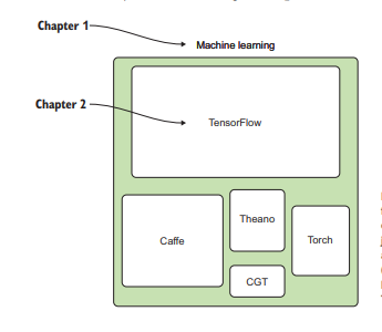
TensorFlow是一个用于机器学习和人工智能的免费和开源的软件库。它可以用于一系列的任务,但特别关注深度神经网络的训练和推理。
statistics-lab™ 为您的留学生涯保驾护航 在代写tensorflow方面已经树立了自己的口碑, 保证靠谱, 高质且原创的统计Statistics代写服务。我们的专家在代写tensorflow代写方面经验极为丰富,各种代写tensorflow相关的作业也就用不着说。
我们提供的tensorflow及其相关学科的代写,服务范围广, 其中包括但不限于:
- Statistical Inference 统计推断
- Statistical Computing 统计计算
- Advanced Probability Theory 高等概率论
- Advanced Mathematical Statistics 高等数理统计学
- (Generalized) Linear Models 广义线性模型
- Statistical Machine Learning 统计机器学习
- Longitudinal Data Analysis 纵向数据分析
- Foundations of Data Science 数据科学基础
机器学习代写|tensorflow代写|Cleaning the data for regression
First, download this data-a set of phone calls from the summer of 2014 from the New York City 311 service-from http://mng.bz/P16w. Kaggle has other 311 datasets, but you’ll use this particular data due to its interesting properties. The calls are formatted as a comma-separated values (CSV) file that has several interesting features, including the following:
- A unique call identifier showing the date when the call was created
” The location and ZIP code of the reported incident or information request - The specific action that the agent on the call took to resolve the issue
- What borough (such as the Bronx or Queens) the call was made from
- The status of the call
This dataset contains lot of useful information for machine learning, but for purposes of this exercise, you care only about the call-creation date. Create a new file named 311.py. Then write a function to read each line in the CSV file, detect the week number, and sum the call counts by week.
Your code will need to deal with some messiness in this data file. First, you aggregate individual calls, sometimes hundreds in a single day, into a seven-day or weekly bin, as identified by the bucket variable in listing 4.1. The freq (short for frequency) variable holds the value of calls per week and per year. If the $311 \mathrm{CSV}$ contains more than a year’s worth of data (as other 311 CSVs that you can find on Kaggle do), gin up your code to allow for selection by year of calls to train on. The result of the code in listing $4.1$ is a freq dictionary whose values are the number of calls indexed by year and by week number via the period variable. The $t$. tm_year variable holds the parsed year resulting from passing the call-creation-time value (indexed in the CSV as date_idx, an integer defining the column number where the date field is located) and the date_parse format string to Python’s time library’s strptime (or string parse time) function. The date parse format string is a pattern defining the way the date appears as text in the CSV so that Python knows how to convert it to a datetime representation.
机器学习代写|tensorflow代写|What’s in a bell curve? Predicting Gaussian distributions
A bell or normal curve is a common term to describe data that we say fits a normal distribution. The largest $Y$ values of the data occur in the middle or statistically the mean $\mathrm{X}$ value of the distribution of points, and the smaller $Y$ values occur on the early and tail X values of the distribution. We also call this a Gaussian distribution after the famous German mathematician Carl Friedrich Gauss, who was responsible for the Gaussian function that describes the normal distribution.
We can use the NumPy method np.random.normal to generate random points sampled from the normal distribution in Python. The following equation shows the Gaussian function that underlies this distribution:
$$
e^{\frac{\left(-(x-\mu)^{2}\right)}{2 \sigma^{2}}}
$$
The equation includes the parameters $\mu$ (pronounced $m u$ ) and $\sigma$ (pronounced sigma), where $m u$ is the mean and sigma is the standard deviation of the distribution, respectively. Mu and sigma are the parameters of the model, and as you have seen, TensorFlow will learn the appropriate values for these parameters as part of training a model.
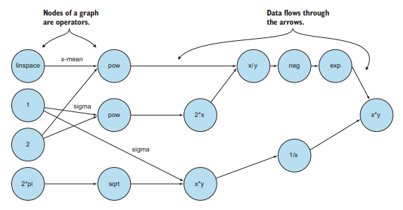
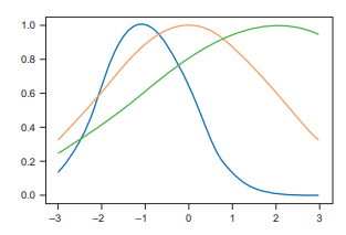
To convince yourself that you can use these parameters to generate bell curves, you can type the code snippet in listing $4.3$ into a file named gaussian.py and then run it to produce the plot that follows it. The code in listing $4.3$ produces the bell curve visualizations shown in figure 4.4. Note that I selected values of mu between $-1$ and 2 . You should see center points of the curve in figure 4.4, as well as standard deviations (sigma) between 1 and 3 , so the width of the curves should correspond to those values inclusively. The code plots 120 linearly-spaced points with $\mathrm{X}$ values between $-3$ and 3 and $\mathrm{Y}$ values between 0 and 1 that fit the normal distribution according to $\mathrm{mu}$ and sigma, and the output should look like figure 4.4.
机器学习代写|tensorflow代写|Training your call prediction regressor
Now you are ready to use TensorFlow to fit your NYC 311 data to this model. It’s probably clear by looking at the curves that they seem to comport naturally with the 311 data, especially if TensorFlow can figure out the values of mu that put the center point of the curve near spring and summer and that have a fairly large call volume, as well as the sigma value that approximates the best standard deviation.
Listing $4.4$ sets up the TensorFlow training session, associated hyperparameters, learning rate, and number of training epochs. I’m using a fairly large step for learning rate so that TensorFlow can appropriately scan the values of mu and sig by taking bigenough steps before settling down. The number of epochs-5,000-gives the algorithm enough training steps to settle on optimal values. In local testing on my laptop, these hyperparameters arrived at strong accuracy $(99 \%)$ and took less than a minute. But I could have chosen other hyperparameters, such as a learning rate of $0.5$, and given the training process more steps (epochs). Part of the fun of machine learning is hyperparameter training, which is more art than science, though techniques such as meta-learning and algorithms such as HyperOpt may ease this process in the future. A full discussion of hyperparameter tuning is beyond the scope of this chapter, but an online search should yields thousands of relevant introductions.
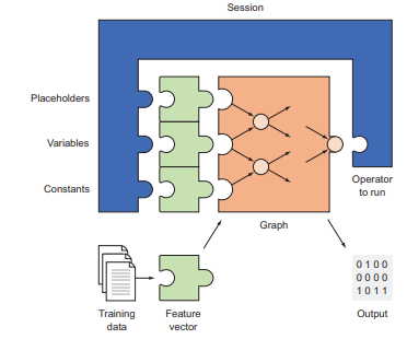
When the hyperparameters are set up, define the placeholders $\mathrm{X}$ and $\mathrm{Y}$, which will be used for the input week number and associated number of calls (normalized), respectively. Earlier, I mentioned normalizing the Y values and creating the ny_train variable in listing $4.2$ to ease learning. The reason is that the model Gaussian function that we are attempting to learn has $\mathrm{Y}$ values only between 0 and 1 due to the exponent e. The model function defines the Gaussian model to learn, with the associated variables mu and sig initialized arbitrarily to 1. The cost function is defined as the L2 norm, and the training uses Gradient descent. After training your regressor for 5,000 epochs, the final steps in listing $4.4$ print the learned values for mu and sig.
tensorflow代考
机器学习代写|tensorflow代写|Polynomial model
线性模型可能是一个直观的初步猜测,但现实世界的相关性很少如此简单。例如,导弹穿过太空的轨迹相对于地球上的观察者是弯曲的。Wi-Fi 信号强度会按照平方反比定律降低。一朵花在其一生中的高度变化肯定不是线性的。
当数据点似乎形成平滑曲线而不是直线时,您需要将回归模型从直线更改为其他模型。一种这样的方法是使用多项式模型。多项式是线性函数的推广。这n次多项式如下所示:
F(X)=在nXn+…+在1X+在0
注意 何时n=1, 多项式只是一个线性方程F(X)=在1X+在0.
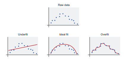
考虑图中的散点图3.10,显示上的输入X-轴和y轴上的输出。如您所知,一条直线不足以描述所有数据。多项式函数是线性函数的更灵活的推广。
机器学习代写|tensorflow代写|Regularization
不要被多项式的奇妙灵活性所迷惑,如部分所示3.3. 仅仅因为高阶多项式是低阶多项式的扩展并不意味着您应该总是更喜欢更灵活的模型。
在现实世界中,原始数据很少形成模拟多项式的平滑曲线。假设您正在绘制一段时间内的房价。数据可能会包含波动。回归的目标是用一个简单的数学方程来表示复杂性。如果您的模型过于灵活,则模型可能会使其对输入的解释过于复杂。
以图 3 .12 中的数据为例。您尝试将八次多项式拟合到似乎遵循等式的点是=X2. 这个过程惨遭失败,因为算法尽力更新多项式的九个系数。
影响学习算法产生更小的系数向量(我们称之为在),您将惩罚添加到损失项中。为了控制你想要衡量惩罚项的重要性,你将惩罚乘以一个恒定的非负数,λ, 如下:
成本(X,是)=失利(X,是)+λ
如果λ设置为 0 ,正则化不起作用。当你设置λ对于越来越大的值,具有较大范数的参数将受到严重惩罚。范数的选择因情况而异,但参数通常由它们的 L1 或 L2 范数来衡量。简而言之,正则化降低了原本容易缠结的模型的一些灵活性。
找出正则化参数的值λ性能最好,您必须将数据集拆分为两个不相交的集合。关于70%随机选择的输入/输出对将由训练数据集组成;剩余的30%将用于测试。您将使用清单中提供的功能3.4用于分割数据集。
机器学习代写|tensorflow代写|Application of linear regression
对虚假数据进行线性回归就像买了一辆新车却从不开车。这个令人敬畏的机器乞求在现实世界中表现出来!幸运的是,网上有很多数据集可以用来测试你新发现的回归知识:
- 马萨诸塞大学阿默斯特分校在 https://scholarworks.umass.edu/data 提供各种类型的小型数据集。
- Kaggle 在 https://www.kaggle.com/datasets 为机器学习竞赛提供所有类型的大规模数据。
= Data.gov (https://catalog.data.gov) 是美国政府的一项开放数据计划,其中包含许多有趣且实用的数据集。
大量数据集包含日期。例如,您可以在 https://www .dropbox.com/s/naw774olqkve7sc/311.csv?dl=0 找到所有拨打加利福尼亚州洛杉矶 311 非紧急热线电话的数据集。一个很好的跟踪功能可能是每天、每周或每月的呼叫频率。为方便起见,列出3.6允许您获取数据项的每周频率计数。
import csv import time
def read(filename, date_idx, date_parse, year, bucket=7)=
days_in_year=365
频率=∣
为范围内的周期设置初始频率图(0, int(days_in year / bucket)):
频率 [期间]=0
使用 open(filename, “rb’) as csvfile: csvreader = csv. 阅读器(csvfile)下一个()
读取csvreader 中行的每个周期的数据和聚合计数:
如果排[date_idx]==′=
继续
吨=time.strptime (row [date_idx], date_parse)
if t.tm_year == year and吨.tm_yday<(days_in_year-1):
频率[int(t.tm_yday / bucket)]+=1
return freq
此代码为您提供线性回归的训练数据。freq 变量是一个字典,它将一个周期(例如一周)映射到一个频率计数。一年有 52 周,因此如果您保持 bucket=7 不变,您将拥有 52 个数据点。

统计代写请认准statistics-lab™. statistics-lab™为您的留学生涯保驾护航。
金融工程代写
金融工程是使用数学技术来解决金融问题。金融工程使用计算机科学、统计学、经济学和应用数学领域的工具和知识来解决当前的金融问题,以及设计新的和创新的金融产品。
非参数统计代写
非参数统计指的是一种统计方法,其中不假设数据来自于由少数参数决定的规定模型;这种模型的例子包括正态分布模型和线性回归模型。
广义线性模型代考
广义线性模型(GLM)归属统计学领域,是一种应用灵活的线性回归模型。该模型允许因变量的偏差分布有除了正态分布之外的其它分布。
术语 广义线性模型(GLM)通常是指给定连续和/或分类预测因素的连续响应变量的常规线性回归模型。它包括多元线性回归,以及方差分析和方差分析(仅含固定效应)。
有限元方法代写
有限元方法(FEM)是一种流行的方法,用于数值解决工程和数学建模中出现的微分方程。典型的问题领域包括结构分析、传热、流体流动、质量运输和电磁势等传统领域。
有限元是一种通用的数值方法,用于解决两个或三个空间变量的偏微分方程(即一些边界值问题)。为了解决一个问题,有限元将一个大系统细分为更小、更简单的部分,称为有限元。这是通过在空间维度上的特定空间离散化来实现的,它是通过构建对象的网格来实现的:用于求解的数值域,它有有限数量的点。边界值问题的有限元方法表述最终导致一个代数方程组。该方法在域上对未知函数进行逼近。[1] 然后将模拟这些有限元的简单方程组合成一个更大的方程系统,以模拟整个问题。然后,有限元通过变化微积分使相关的误差函数最小化来逼近一个解决方案。
tatistics-lab作为专业的留学生服务机构,多年来已为美国、英国、加拿大、澳洲等留学热门地的学生提供专业的学术服务,包括但不限于Essay代写,Assignment代写,Dissertation代写,Report代写,小组作业代写,Proposal代写,Paper代写,Presentation代写,计算机作业代写,论文修改和润色,网课代做,exam代考等等。写作范围涵盖高中,本科,研究生等海外留学全阶段,辐射金融,经济学,会计学,审计学,管理学等全球99%专业科目。写作团队既有专业英语母语作者,也有海外名校硕博留学生,每位写作老师都拥有过硬的语言能力,专业的学科背景和学术写作经验。我们承诺100%原创,100%专业,100%准时,100%满意。
随机分析代写
随机微积分是数学的一个分支,对随机过程进行操作。它允许为随机过程的积分定义一个关于随机过程的一致的积分理论。这个领域是由日本数学家伊藤清在第二次世界大战期间创建并开始的。
时间序列分析代写
随机过程,是依赖于参数的一组随机变量的全体,参数通常是时间。 随机变量是随机现象的数量表现,其时间序列是一组按照时间发生先后顺序进行排列的数据点序列。通常一组时间序列的时间间隔为一恒定值(如1秒,5分钟,12小时,7天,1年),因此时间序列可以作为离散时间数据进行分析处理。研究时间序列数据的意义在于现实中,往往需要研究某个事物其随时间发展变化的规律。这就需要通过研究该事物过去发展的历史记录,以得到其自身发展的规律。
回归分析代写
多元回归分析渐进(Multiple Regression Analysis Asymptotics)属于计量经济学领域,主要是一种数学上的统计分析方法,可以分析复杂情况下各影响因素的数学关系,在自然科学、社会和经济学等多个领域内应用广泛。
MATLAB代写
MATLAB 是一种用于技术计算的高性能语言。它将计算、可视化和编程集成在一个易于使用的环境中,其中问题和解决方案以熟悉的数学符号表示。典型用途包括:数学和计算算法开发建模、仿真和原型制作数据分析、探索和可视化科学和工程图形应用程序开发,包括图形用户界面构建MATLAB 是一个交互式系统,其基本数据元素是一个不需要维度的数组。这使您可以解决许多技术计算问题,尤其是那些具有矩阵和向量公式的问题,而只需用 C 或 Fortran 等标量非交互式语言编写程序所需的时间的一小部分。MATLAB 名称代表矩阵实验室。MATLAB 最初的编写目的是提供对由 LINPACK 和 EISPACK 项目开发的矩阵软件的轻松访问,这两个项目共同代表了矩阵计算软件的最新技术。MATLAB 经过多年的发展,得到了许多用户的投入。在大学环境中,它是数学、工程和科学入门和高级课程的标准教学工具。在工业领域,MATLAB 是高效研究、开发和分析的首选工具。MATLAB 具有一系列称为工具箱的特定于应用程序的解决方案。对于大多数 MATLAB 用户来说非常重要,工具箱允许您学习和应用专业技术。工具箱是 MATLAB 函数(M 文件)的综合集合,可扩展 MATLAB 环境以解决特定类别的问题。可用工具箱的领域包括信号处理、控制系统、神经网络、模糊逻辑、小波、仿真等。