分类：泛函分析作业代写

数学代写|泛函分析作业代写Functional Analysis代考|Math255A

Posted on 2023年8月25日2023年8月25日 by statistics-lab

如果你也在怎样代写泛函分析functional analysis 这个学科遇到相关的难题，请随时右上角联系我们的24/7代写客服。泛函分析functional analysis部分利用局部凸空间理论中的各种技术来解决解析问题，由于范畴论和同调代数等相关课题的新发展。

泛函分析functional analysis得到了很大的发展。特别是，关于衍生的射影极限函子(它测量阻碍从局部解构造问题的整体解的障碍)和fr和更一般空间的分裂理论(它关注解算子的存在性)的进展允许新的应用，例如关于偏微分算子或卷积算子的问题。

statistics-lab™ 为您的留学生涯保驾护航在代写泛函分析Functional Analysis方面已经树立了自己的口碑, 保证靠谱, 高质且原创的统计Statistics代写服务。我们的专家在代写泛函分析Functional Analysis代写方面经验极为丰富，各种代写泛函分析Functional Analysis相关的作业也就用不着说。

数学代写|泛函分析作业代写Functional Analysis代考|Math255A

数学代写|泛函分析作业代写Functional Analysis代考|Energy Spaces

We have already introduced the energy space for a string. Let us consider other examples. In what follows, we shall employ only dimensionless variables, parameters, and functions of state of a body.
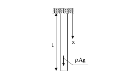
Bending of a Bar
In the Introduction we considered the problem of bending a clamped bar, which was governed by (4). The potential energy of the bar is
$$
\mathcal{E}_1(y)=\frac{1}{2} \int_0^l B(x)\left(y^{\prime \prime}\right)^2 d x .
$$
On the set $S$ consisting of all functions $y(x)$ that are twice continuously differentiable on $[0, l]$ and that satisfy
$$
y(0)=y^{\prime}(0)=y(l)=y^{\prime}(l)=0,
$$
let us consider
$$
d\left(y_1, y_2\right)=\left(2 \mathcal{E}_1\left(y_1-y_2\right)\right)^{1 / 2}=\left(\int_0^l B(x)\left[y_1^{\prime \prime}(x)-y_2^{\prime \prime}(x)\right]^2 d x\right)^{1 / 2} .
$$
For this, D1 and D3 obviously hold. Satisfaction of D4 follows from the fact that $\mathcal{E}_1(y)$ is quadratic in $y$. To verify D2, we need only show that $d(y, z)=0$ implies $y(x)=z(x)$. But $d(y, z)=0$ implies $(y(x)-z(x))^{\prime \prime}=0$, hence $y(x)-z(x)=a_1 x+a_2$ where $a_1, a_2$ are constants; imposing (1.3.1), we arrive at $a_1=a_2=0$. So $d\left(y_1, y_2\right)$ is indeed a metric on $S$.

The potential energy of a membrane occupying a domain $\Omega \subset \mathbb{R}^2$ is proportional to
$$
\mathcal{E}2(u)=\int{\Omega}\left[\left(\frac{\partial u}{\partial x}\right)^2+\left(\frac{\partial u}{\partial y}\right)^2\right] d x d y .
$$
So we can try
$$
d(u, v)=\left(\mathcal{E}2(u-v)\right)^{1 / 2} $$ as a metric on the functions $u=u(x, y)$ that describe the normal displacements of the membrane. We first consider the case where the edge of the membrane is clamped, i.e., $$ \left.u\right|{\partial \Omega}=0
$$
where $\partial \Omega$ is the boundary of $\Omega$. The function $d(u, v)$ of (1.3.2) is a metric on the set $C^{(1)}(\Omega)$. Axioms D1 and D3 hold obviously; D2 holds by (1.3.3), and D4 holds by the quadratic nature of $\mathcal{E}2(u)$. This space is appropriate for investigating the corresponding boundary value problem $$ \Delta u=-f,\left.\quad u\right|{\partial \Omega}=0,
$$
called the Dirichlet problem for Poisson’s equation. This describes the behavior of the clamped membrane under a load $f=f(x, y)$.

数学代写|泛函分析作业代写Functional Analysis代考|A Plate

For a linear elastic plate the potential energy is
$$
\mathcal{E}3(w)=\int{\Omega} \frac{D}{2}\left{(\Delta w)^2+2(1-\nu)\left[\left(\frac{\partial^2 w}{\partial x \partial y}\right)^2-\frac{\partial^2 w}{\partial x^2} \frac{\partial^2 w}{\partial y^2}\right]\right} d x d y
$$
where $D$ is the bending stiffness of the plate, $\nu$ is Poisson’s ratio, and $w(x, y)$ is the normal displacement of the mid-surface of the plate, which is denoted by $\Omega$ in the $x y$-plane. If the edge of the plate is clamped we get
$$
\left.w\right|{\partial \Omega}=\left.\frac{\partial w}{\partial n}\right|{\partial \Omega}=0 .
$$
If $\mathcal{E}_3(w)=0$, then $w=a+b x+c y$ and, from (1.3.7), $w=0$. So D2 is fulfilled by the distance function
$$
d\left(w_1, w_2\right)=\left(2 \mathcal{E}_3\left(w_1-w_2\right)\right)^{1 / 2} .
$$
The remaining metric axioms are easily checked, and $d\left(w_1, w_2\right)$ is a metric on the subset of $C^{(2)}(\Omega)$ consisting of all functions satisfying (1.3.7). This is the energy space for the plate.

If the edge of the plate is free from geometrical fixing (clamping), the situation is similar to the Neumann problem of membrane theory: we must eliminate “rigid” motions of the plate. We shall consider this in detail later.

泛函分析代写

数学代写|泛函分析作业代写Functional Analysis代考|Energy Spaces

我们已经介绍了弦的能量空间。让我们考虑其他例子。在下文中，我们将只使用一个物体的无量纲变量、参数和状态函数。
杆的弯曲
在引言中，我们考虑了夹紧杆的弯曲问题，该问题由式(4)决定
$$
\mathcal{E}_1(y)=\frac{1}{2} \int_0^l B(x)\left(y^{\prime \prime}\right)^2 d x .
$$
在集合$S$上包含所有在$[0, l]$上两次连续可微的函数$y(x)$并且满足
$$
y(0)=y^{\prime}(0)=y(l)=y^{\prime}(l)=0,
$$
让我们考虑一下
$$
d\left(y_1, y_2\right)=\left(2 \mathcal{E}_1\left(y_1-y_2\right)\right)^{1 / 2}=\left(\int_0^l B(x)\left[y_1^{\prime \prime}(x)-y_2^{\prime \prime}(x)\right]^2 d x\right)^{1 / 2} .
$$
对于这个，D1和D3显然成立。D4的满足是由于$\mathcal{E}_1(y)$在$y$中是二次的。为了验证D2，我们只需要证明$d(y, z)=0$意味着$y(x)=z(x)$。但$d(y, z)=0$意味着$(y(x)-z(x))^{\prime \prime}=0$，因此$y(x)-z(x)=a_1 x+a_2$，其中$a_1, a_2$是常数;通过(1.3.1)，我们得到$a_1=a_2=0$。所以$d\left(y_1, y_2\right)$实际上是$S$的一个度量。

占据一个区域的膜的势能$\Omega \subset \mathbb{R}^2$与
$$
\mathcal{E}2(u)=\int{\Omega}\left[\left(\frac{\partial u}{\partial x}\right)^2+\left(\frac{\partial u}{\partial y}\right)^2\right] d x d y .
$$
所以我们可以试试
$$
d(u, v)=\left(\mathcal{E}2(u-v)\right)^{1 / 2} $$作为描述膜的正常位移的函数$u=u(x, y)$的度量。我们首先考虑膜的边缘被夹住的情况，即$$ \left.u\right|{\partial \Omega}=0
$$
其中$\partial \Omega$为$\Omega$的边界。(1.3.2)的函数$d(u, v)$是集$C^{(1)}(\Omega)$上的度量。公理D1和D3显然成立;D2由(1.3.3)成立，D4由$\mathcal{E}2(u)$的二次性质成立。这个空间适合于研究相应的边值问题$$ \Delta u=-f,\left.\quad u\right|{\partial \Omega}=0,
$$
叫做泊松方程的狄利克雷问题。这描述了夹紧膜在负载$f=f(x, y)$下的行为。

数学代写|泛函分析作业代写Functional Analysis代考|A Plate

对于线弹性板，势能为
$$
\mathcal{E}3(w)=\int{\Omega} \frac{D}{2}\left{(\Delta w)^2+2(1-\nu)\left[\left(\frac{\partial^2 w}{\partial x \partial y}\right)^2-\frac{\partial^2 w}{\partial x^2} \frac{\partial^2 w}{\partial y^2}\right]\right} d x d y
$$
式中$D$为板的抗弯刚度，$\nu$为泊松比，$w(x, y)$为板中表面的法向位移，在$x y$ -平面中用$\Omega$表示。如果盘子的边缘被夹住，我们就得到
$$
\left.w\right|{\partial \Omega}=\left.\frac{\partial w}{\partial n}\right|{\partial \Omega}=0 .
$$
如果为$\mathcal{E}_3(w)=0$，则为$w=a+b x+c y$，从(1.3.7)中得到$w=0$。D2由距离函数满足
$$
d\left(w_1, w_2\right)=\left(2 \mathcal{E}_3\left(w_1-w_2\right)\right)^{1 / 2} .
$$
其余的度量公理很容易检查，$d\left(w_1, w_2\right)$是$C^{(2)}(\Omega)$子集上的一个度量，该子集由满足(1.3.7)的所有函数组成。这是平板的能量空间。

如果板的边缘没有几何固定(夹紧)，情况类似于膜理论的诺伊曼问题:我们必须消除板的“刚性”运动。我们稍后将详细考虑这一点。

数学代写|泛函分析作业代写Functional Analysis代考请认准statistics-lab™

统计代写请认准statistics-lab™. statistics-lab™为您的留学生涯保驾护航。

金融工程代写

金融工程是使用数学技术来解决金融问题。金融工程使用计算机科学、统计学、经济学和应用数学领域的工具和知识来解决当前的金融问题，以及设计新的和创新的金融产品。

非参数统计代写

非参数统计指的是一种统计方法，其中不假设数据来自于由少数参数决定的规定模型；这种模型的例子包括正态分布模型和线性回归模型。

广义线性模型代考

广义线性模型（GLM）归属统计学领域，是一种应用灵活的线性回归模型。该模型允许因变量的偏差分布有除了正态分布之外的其它分布。

术语广义线性模型（GLM）通常是指给定连续和/或分类预测因素的连续响应变量的常规线性回归模型。它包括多元线性回归，以及方差分析和方差分析（仅含固定效应）。

有限元方法代写

有限元方法（FEM）是一种流行的方法，用于数值解决工程和数学建模中出现的微分方程。典型的问题领域包括结构分析、传热、流体流动、质量运输和电磁势等传统领域。

有限元是一种通用的数值方法，用于解决两个或三个空间变量的偏微分方程（即一些边界值问题）。为了解决一个问题，有限元将一个大系统细分为更小、更简单的部分，称为有限元。这是通过在空间维度上的特定空间离散化来实现的，它是通过构建对象的网格来实现的：用于求解的数值域，它有有限数量的点。边界值问题的有限元方法表述最终导致一个代数方程组。该方法在域上对未知函数进行逼近。[1] 然后将模拟这些有限元的简单方程组合成一个更大的方程系统，以模拟整个问题。然后，有限元通过变化微积分使相关的误差函数最小化来逼近一个解决方案。

tatistics-lab作为专业的留学生服务机构，多年来已为美国、英国、加拿大、澳洲等留学热门地的学生提供专业的学术服务，包括但不限于Essay代写，Assignment代写，Dissertation代写，Report代写，小组作业代写，Proposal代写，Paper代写，Presentation代写，计算机作业代写，论文修改和润色，网课代做，exam代考等等。写作范围涵盖高中，本科，研究生等海外留学全阶段，辐射金融，经济学，会计学，审计学，管理学等全球99%专业科目。写作团队既有专业英语母语作者，也有海外名校硕博留学生，每位写作老师都拥有过硬的语言能力，专业的学科背景和学术写作经验。我们承诺100%原创，100%专业，100%准时，100%满意。

随机分析代写

随机微积分是数学的一个分支，对随机过程进行操作。它允许为随机过程的积分定义一个关于随机过程的一致的积分理论。这个领域是由日本数学家伊藤清在第二次世界大战期间创建并开始的。

时间序列分析代写

随机过程，是依赖于参数的一组随机变量的全体，参数通常是时间。随机变量是随机现象的数量表现，其时间序列是一组按照时间发生先后顺序进行排列的数据点序列。通常一组时间序列的时间间隔为一恒定值（如1秒，5分钟，12小时，7天，1年），因此时间序列可以作为离散时间数据进行分析处理。研究时间序列数据的意义在于现实中，往往需要研究某个事物其随时间发展变化的规律。这就需要通过研究该事物过去发展的历史记录，以得到其自身发展的规律。

回归分析代写

多元回归分析渐进（Multiple Regression Analysis Asymptotics）属于计量经济学领域，主要是一种数学上的统计分析方法，可以分析复杂情况下各影响因素的数学关系，在自然科学、社会和经济学等多个领域内应用广泛。

MATLAB代写

MATLAB 是一种用于技术计算的高性能语言。它将计算、可视化和编程集成在一个易于使用的环境中，其中问题和解决方案以熟悉的数学符号表示。典型用途包括：数学和计算算法开发建模、仿真和原型制作数据分析、探索和可视化科学和工程图形应用程序开发，包括图形用户界面构建MATLAB 是一个交互式系统，其基本数据元素是一个不需要维度的数组。这使您可以解决许多技术计算问题，尤其是那些具有矩阵和向量公式的问题，而只需用 C 或 Fortran 等标量非交互式语言编写程序所需的时间的一小部分。MATLAB 名称代表矩阵实验室。MATLAB 最初的编写目的是提供对由 LINPACK 和 EISPACK 项目开发的矩阵软件的轻松访问，这两个项目共同代表了矩阵计算软件的最新技术。MATLAB 经过多年的发展，得到了许多用户的投入。在大学环境中，它是数学、工程和科学入门和高级课程的标准教学工具。在工业领域，MATLAB 是高效研究、开发和分析的首选工具。MATLAB 具有一系列称为工具箱的特定于应用程序的解决方案。对于大多数 MATLAB 用户来说非常重要，工具箱允许您学习和应用专业技术。工具箱是 MATLAB 函数（M 文件）的综合集合，可扩展 MATLAB 环境以解决特定类别的问题。可用工具箱的领域包括信号处理、控制系统、神经网络、模糊逻辑、小波、仿真等。

R语言代写	问卷设计与分析代写
PYTHON代写	回归分析与线性模型代写
MATLAB代写	方差分析与试验设计代写
STATA代写	机器学习/统计学习代写
SPSS代写	计量经济学代写
EVIEWS代写	时间序列分析代写
EXCEL代写	深度学习代写
SQL代写	各种数据建模与可视化代写

数学代写|泛函分析作业代写Functional Analysis代考|MATH784

Posted on 2023年8月25日2023年8月25日 by statistics-lab

数学代写|泛函分析作业代写Functional Analysis代考|Preliminaries

Consider a set of particles $P_i, i=1, \ldots, n$. To locate these particles in the space $\mathbb{R}^3$, we need a reference system. Let the Cartesian coordinates of $P_i$ be $\left(\xi_i, \eta_i, \zeta_i\right)$ for each $i$. Identifying $\left(\xi_1, \eta_1, \zeta_1\right)$ with $\left(x_1, x_2, x_3\right),\left(\xi_2, \eta_2, \zeta_2\right)$ with $\left(x_4, x_5, x_6\right)$, and so on, we obtain a vector $\mathbf{x}$ of the Euclidean space $\mathbb{R}^{3 n}$ with coordinates $\left(x_1, x_2, \ldots, x_{3 n}\right)$. This vector determines the positions of all particles in the set.

To distinguish different configurations $\mathbf{x}$ and $\mathbf{y}$ of the system, we can introduce a distance from $\mathbf{x}$ to $\mathbf{y}$ :
$$
d_E(\mathbf{x}, \mathbf{y})=\left(\sum_{i=1}^{3 n}\left(x_i-y_i\right)^2\right)^{1 / 2} .
$$
This is the Euclidean distance (or metric) of $\mathbb{R}^{3 n}$. Alternatively, we could characterize the distance from $\mathbf{x}$ to $\mathbf{y}$ using the function
$$
d_S(\mathbf{x}, \mathbf{y})=\max \left{\left|x_1-y_1\right|,\left|x_2-y_2\right|, \ldots,\left|x_{3 n}-y_{3 n}\right|\right} .
$$
It is easily seen that each of the metrics $d_E$ and $d_S$ satisfy the following properties, known as the metric axioms:
D1. $d(\mathbf{x}, \mathbf{y}) \geq 0$;
D2. $d(\mathbf{x}, \mathbf{y})=0$ if and only if $\mathbf{x}=\mathbf{y}$;

D3. $d(\mathbf{x}, \mathbf{y})=d(\mathbf{y}, \mathbf{x})$;
D4. $d(\mathbf{x}, \mathbf{y}) \leq d(\mathbf{x}, \mathbf{z})+d(\mathbf{z}, \mathbf{y})$.
Any real valued function $d(\mathbf{x}, \mathbf{y})$ defined for all $\mathbf{x}, \mathbf{y} \in \mathbb{R}^{3 n}$ is called a metric on $\mathbb{R}^{3 n}$ if it satisfies properties D1-D4. Property D1 is called the axiom of positiveness, property D3 is called the axiom of symmetry, and property D4 is called the triangle inequality.

数学代写|泛函分析作业代写Functional Analysis代考|Some Metric Spaces of Functions

To describe the behavior or change in state of a body in space, we use functions of one or more variables. Displacements, velocities, loads, and temperatures are all functions of position. So we must learn how to distinguish different states of a body; the appropriate tool for this is, of course, the notion of metric space. In mechanics of materials, we deal mostly with real-valued continuous or differentiable functions.

Let $\Omega$ be a closed and bounded domain in $\mathbb{R}^n$. A natural measure of the deviation between two continuous functions $f(\mathbf{x})$ and $g(\mathbf{x}), \mathbf{x} \in \Omega$, is
$$
d(f, g)=\max {\mathbf{x} \in \Omega}|f(\mathbf{x})-g(\mathbf{x})| . $$ It is obvious that $d(f, g)$ satisfies axioms D1-D3. Let us verify D4. Since $|f(\mathbf{x})-g(\mathbf{x})|$ is a continuous function on $\Omega$, there exists a point $\mathbf{x}_0 \in \Omega$ such that $$ d(f, g)=\max {\mathbf{x} \in \Omega}|f(\mathbf{x})-g(\mathbf{x})|=\left|f\left(\mathbf{x}_0\right)-g\left(\mathbf{x}_0\right)\right| .
$$
For any function $h(\mathbf{x})$ which is continuous on $\Omega$, we get
$$
\begin{aligned}
d(f, g) & =\left|f\left(\mathbf{x}_0\right)-g\left(\mathbf{x}_0\right)\right| \
& \leq\left|f\left(\mathbf{x}_0\right)-h\left(\mathbf{x}_0\right)\right|+\left|h\left(\mathbf{x}_0\right)-g\left(\mathbf{x}_0\right)\right| \
& \leq d(f, h)+d(h, g) .
\end{aligned}
$$
(Here we use the Weierstrass theorem that on a compact set a continuous function attains its maximum and minimum values.) Thus $d(f, g)$ in (1.2.1) is a metric.

泛函分析代写

数学代写|泛函分析作业代写Functional Analysis代考|Preliminaries

考虑一组粒子$P_i, i=1, \ldots, n$。为了在空间$\mathbb{R}^3$中定位这些粒子，我们需要一个参考系统。设$P_i$的笛卡尔坐标为$\left(\xi_i, \eta_i, \zeta_i\right)$对于每个$i$。将$\left(\xi_1, \eta_1, \zeta_1\right)$与$\left(x_1, x_2, x_3\right),\left(\xi_2, \eta_2, \zeta_2\right)$与$\left(x_4, x_5, x_6\right)$等同，以此类推，我们得到坐标为$\left(x_1, x_2, \ldots, x_{3 n}\right)$的欧几里得空间$\mathbb{R}^{3 n}$的向量$\mathbf{x}$。这个向量决定了集合中所有粒子的位置。

为了区分系统的不同配置$\mathbf{x}$和$\mathbf{y}$，我们可以引入$\mathbf{x}$到$\mathbf{y}$之间的距离:
$$
d_E(\mathbf{x}, \mathbf{y})=\left(\sum_{i=1}^{3 n}\left(x_i-y_i\right)^2\right)^{1 / 2} .
$$
这是$\mathbb{R}^{3 n}$的欧氏距离(或度规)或者，我们可以使用函数描述从$\mathbf{x}$到$\mathbf{y}$的距离
$$
d_S(\mathbf{x}, \mathbf{y})=\max \left{\left|x_1-y_1\right|,\left|x_2-y_2\right|, \ldots,\left|x_{3 n}-y_{3 n}\right|\right} .
$$
很容易看出，每个度量$d_E$和$d_S$都满足以下性质，称为度量公理:
d。$d(\mathbf{x}, \mathbf{y}) \geq 0$;
d。$d(\mathbf{x}, \mathbf{y})=0$当且仅当$\mathbf{x}=\mathbf{y}$;

d3。$d(\mathbf{x}, \mathbf{y})=d(\mathbf{y}, \mathbf{x})$;
d4;$d(\mathbf{x}, \mathbf{y}) \leq d(\mathbf{x}, \mathbf{z})+d(\mathbf{z}, \mathbf{y})$。
对于所有$\mathbf{x}, \mathbf{y} \in \mathbb{R}^{3 n}$定义的任何实值函数$d(\mathbf{x}, \mathbf{y})$，如果满足属性D1-D4，则称为$\mathbb{R}^{3 n}$上的度量。性质D1称为正性公理，性质D3称为对称公理，性质D4称为三角形不等式。

数学代写|泛函分析作业代写Functional Analysis代考|Some Metric Spaces of Functions

为了描述物体在空间中的行为或状态变化，我们使用一个或多个变量的函数。位移、速度、载荷和温度都是位置的函数。所以我们必须学会如何区分身体的不同状态;合适的工具当然是度量空间的概念。在材料力学中，我们主要处理实值连续函数或可微函数。

设$\Omega$为$\mathbb{R}^n$中的封闭有界域。两个连续函数$f(\mathbf{x})$和$g(\mathbf{x}), \mathbf{x} \in \Omega$之间的偏差的自然度量是
$$
d(f, g)=\max {\mathbf{x} \in \Omega}|f(\mathbf{x})-g(\mathbf{x})| . $$很明显，$d(f, g)$满足公理D1-D3。让我们验证D4。由于$|f(\mathbf{x})-g(\mathbf{x})|$是$\Omega$上的连续函数，因此存在一个点$\mathbf{x}_0 \in \Omega$，使得$$ d(f, g)=\max {\mathbf{x} \in \Omega}|f(\mathbf{x})-g(\mathbf{x})|=\left|f\left(\mathbf{x}_0\right)-g\left(\mathbf{x}_0\right)\right| .
$$
对于任意在$\Omega$上连续的函数$h(\mathbf{x})$，我们得到
$$
\begin{aligned}
d(f, g) & =\left|f\left(\mathbf{x}_0\right)-g\left(\mathbf{x}_0\right)\right| \
& \leq\left|f\left(\mathbf{x}_0\right)-h\left(\mathbf{x}_0\right)\right|+\left|h\left(\mathbf{x}_0\right)-g\left(\mathbf{x}_0\right)\right| \
& \leq d(f, h)+d(h, g) .
\end{aligned}
$$
(这里我们使用Weierstrass定理，即在紧集合上连续函数达到最大值和最小值。)因此(1.2.1)中的$d(f, g)$是一个度量。

统计代写请认准statistics-lab™. statistics-lab™为您的留学生涯保驾护航。

金融工程代写

非参数统计代写

非参数统计指的是一种统计方法，其中不假设数据来自于由少数参数决定的规定模型；这种模型的例子包括正态分布模型和线性回归模型。

广义线性模型代考

广义线性模型（GLM）归属统计学领域，是一种应用灵活的线性回归模型。该模型允许因变量的偏差分布有除了正态分布之外的其它分布。

有限元方法代写

随机分析代写

时间序列分析代写

回归分析代写

MATLAB代写

R语言代写	问卷设计与分析代写
PYTHON代写	回归分析与线性模型代写
MATLAB代写	方差分析与试验设计代写
STATA代写	机器学习/统计学习代写
SPSS代写	计量经济学代写
EVIEWS代写	时间序列分析代写
EXCEL代写	深度学习代写
SQL代写	各种数据建模与可视化代写

数学代写|泛函分析作业代写Functional Analysis代考|MAT4450

Posted on 2023年8月25日2023年8月25日 by statistics-lab

数学代写|泛函分析作业代写Functional Analysis代考|MATH510

数学代写|泛函分析作业代写Functional Analysis代考|Inductive spectra of locally convex spaces

Given an inductive spectrum $\left(X_n\right)n$ there is a canonical algebraically exact sequence $$ 0 \longrightarrow \bigoplus{n \in \mathbb{N}} X_n \stackrel{d}{\longrightarrow} \bigoplus_{n \in \mathbb{N}} X_n \stackrel{\sigma}{\longrightarrow} X \longrightarrow 0
$$
where $d\left(\left(x_n\right){n \in \mathbb{N}}\right)=\left(x_n-x{n-1}\right){n \in \mathbb{N}}, x_0=0$, and $\sigma\left(\left(x_n\right){n \in \mathbb{N}}\right)=\sum_{n \in \mathbb{N}} x_n$.
$d$ and $\sigma$ are continuous, and $\sigma$ is also open. The spectrum is called (weakly) acyclic if $d$ is (weakly) open onto its range.

This definition is related to the question whether a subspace $L$ of an inductive limit ind $X_n$ is topologically the inductive limit of the spaces $L_n=X \cap L_n$ (in this case $L$ is called a limit subspace) or if it has at least the same topological dual as the inductive limit (then $L$ is called well-located). Using either the duality explained below or a diagram chase on gets:
A subspace $L$ of the limit $X=\operatorname{ind} X_n$ of a (weakly) acyclic inductive spectrum is (well-located) a limit subspace if and only if the spectrum $\left(X_n / L_n\right)_{n \in \mathbb{N}}$ is (weakly) acyclic.

An easy calculation shows that the transposed of $d$ is
$$
\Psi: \prod_{n \in \mathbb{N}} X_n^{\prime} \longrightarrow \prod_{n \in \mathbb{N}} X_n^{\prime},\left(f_n\right){n \in \mathbb{N}} \longmapsto\left(f_n-\varrho{n+1}^n\left(f_{n+1}\right)\right){n \in \mathbb{N}} $$ where $\varrho{n+1}^n: X_{n+1}^{\prime} \longrightarrow X_n^{\prime}$ is the restriction (i.e. the transposed of the inclusion). Thus, there is a close connection between (weakly) acyclic inductive spectra and the derived projective limit functor. In particular, an inductive spectrum $\left(X_n\right)_{n \in \mathbb{N}}$ is weakly acyclic if and only if $\operatorname{Proj}^1 \mathscr{Y}=0$ where $\mathscr{Y}=\left(X_n^{\prime}, \varrho_m^n\right)$ with the restrictions as spectral maps. Thus, the results of chapter 3 have immediate counterparts for weakly acyclic spectra which we do not state explicitely.

There is also a direct relation between acyclic inductive spectra and properties of projective limits. Using theorem 2.2 .2 we obtain that $\left(X_n\right){n \in \mathbb{N}}$ is acyclic if and only if for every set $I$ we have $\operatorname{Proj}^1\left(L\left(X_n, \ell_I^{\infty}\right), R_m^n\right)=0$ where $R{n+1}^n(T)=T \circ \varrho_{n+1}^n$. The spaces $L\left(X_n, \ell_I^{\infty}\right)$ are covered by the system $\left{\left(U^{\circ}\right)^I: U \in \mathscr{U}0\left(X_n\right)\right}$ (here, we identify $T \in L\left(X_n, \ell_I^{\infty}\right)$ with a family $\left.\left(T_i\right){i \in I}\right)$ and using theorem 3.2 .14 and the remark following its proof we obtain a general sufficient condition for acyclicity (a direct proof of this can be obtained as in [69]).

数学代写|泛函分析作业代写Functional Analysis代考|The duality functor

This final chapter is concerned with the problem when the transposed map of a homomorphism in the category of locally convex spaces is again a homomorphism. Let
$$
0 \longrightarrow X \stackrel{f}{\longrightarrow} Y \stackrel{g}{\longrightarrow} Z \longrightarrow 0
$$
be an exact sequence in the category of locally convex spaces. The HahnBanach theorem implies that the dual sequence
$$
0 \longrightarrow Z^{\prime} \stackrel{g^t}{\longrightarrow} Y^{\prime} \stackrel{f^t}{\longrightarrow} X^{\prime} \longrightarrow 0
$$
is exact as a sequence of vector spaces, but if all duals are endowed with the strong topology neither $f^t$ nor $g^t$ must be a homomorphism. Let $D$ be the contravariant functor assigning to a locally convex space $X$ its strong dual $X_\beta^{\prime}$ and to $f: X \longrightarrow Y$ the transposed map. Then an exact complex
$$
0 \longrightarrow X \longrightarrow Y \longrightarrow Z \longrightarrow 0
$$
is transformed into an acyclic complex
$$
0 \longrightarrow D(Z) \longrightarrow D(Y) \longrightarrow D(X) \longrightarrow 0
$$
To measure the exactness of this complex Palamodov used the functors $H_M$ introduced in section 2.2. For any non-empty set $M$ we define the covariant functor $D_M=H_M \circ D$ from $\mathcal{L C S}$ to the category of vector spaces. Explicitely, to a locally convex space $X$ we $\operatorname{assign} D_M(X)=\operatorname{Hom}\left(X_\beta^{\prime}, \ell_M^{\infty}\right)$, and for a morphism $f: X \longrightarrow Y$ the linear map
$$
f^*=D_M(f): \operatorname{Hom}\left(X_\beta^{\prime}, \ell_M^{\infty}\right) \longrightarrow \operatorname{Hom}\left(Y_\beta^{\prime}, \ell_M^{\infty}\right)
$$
is defined by $T \mapsto T \circ f^t$. From theorem 2.2.2 we deduce that for an exact sequence
$$
0 \longrightarrow X \stackrel{f}{\longrightarrow} Y \stackrel{g}{\longrightarrow} Z \longrightarrow 0
$$

the dual sequence
$$
0 \longrightarrow X^{\prime} \stackrel{g^t}{\longrightarrow} Y^{\prime} \stackrel{f^t}{\longrightarrow} X^{\prime} \longrightarrow 0
$$
is left exact at $Y^{\prime}$ (i.e. $g^t$ is open onto its range) or right exact at $Y^{\prime}$ (i.e. $f^t$ is open) respectively if and only if for every set $M \neq \emptyset$ the complex
$$
0 \longrightarrow D_M(X) \stackrel{f^}{\longrightarrow} D_M(Y) \stackrel{g^}{\longrightarrow} D_M(Z) \longrightarrow 0
$$
is exact at $D_M(Z)$ or exact at $D_M(Y)$, respectively. (We note that the complex is always exact at $D_M(X)$, i.e. $D_M$ is a semi-injective functor.) The exactness at $D_M(Z)$ and $D_M(Y)$ are measured by $D_M^1(X)$ and $D_M^{+}(X)$, respectively. Let us recall the definitions of $D_M^1$ and $D_M^{+}$. If
$$
0 \longrightarrow X \stackrel{i}{\longrightarrow} I_0 \stackrel{i_1}{\longrightarrow} I_1 \stackrel{i_2}{\longrightarrow} \ldots
$$
is any injective resolution of $X$ we have
$$
\begin{gathered}
D_M^{+}(X)=\operatorname{ker} D_M\left(i_0\right) / \operatorname{im} D_M(i) \text { and } \
D_M^1(X)=\operatorname{ker} D_M\left(i_1\right) / \operatorname{im} D_M\left(i_0\right) .
\end{gathered}
$$

数学代写|泛函分析作业代写Functional Analysis代考|MAT4450

泛函分析代写

数学代写|泛函分析作业代写Functional Analysis代考|Inductive spectra of locally convex spaces

给定一个归纳谱$\left(X_n\right)n$，有一个正则代数精确序列$$ 0 \longrightarrow \bigoplus{n \in \mathbb{N}} X_n \stackrel{d}{\longrightarrow} \bigoplus_{n \in \mathbb{N}} X_n \stackrel{\sigma}{\longrightarrow} X \longrightarrow 0
$$
其中$d\left(\left(x_n\right){n \in \mathbb{N}}\right)=\left(x_n-x{n-1}\right){n \in \mathbb{N}}, x_0=0$和$\sigma\left(\left(x_n\right){n \in \mathbb{N}}\right)=\sum_{n \in \mathbb{N}} x_n$。
$d$和$\sigma$是连续的，$\sigma$也是开放的。如果$d$在其范围内(弱)开放，则称为(弱)无环谱。

这个定义与以下问题有关:一个归纳极限和$X_n$的子空间$L$是否在拓扑上是空间$L_n=X \cap L_n$的归纳极限(在这种情况下$L$被称为极限子空间)，或者它是否至少与归纳极限具有相同的拓扑对偶(那么$L$被称为定位良好)。使用下面解释的对偶性或使用图表追踪gets:
当且仅当(弱)无环电感谱$\left(X_n / L_n\right)_{n \in \mathbb{N}}$是(弱)无环时，其极限$X=\operatorname{ind} X_n$的子空间$L$是(定位良好的)极限子空间。

一个简单的计算表明$d$的转置是
$$
\Psi: \prod_{n \in \mathbb{N}} X_n^{\prime} \longrightarrow \prod_{n \in \mathbb{N}} X_n^{\prime},\left(f_n\right){n \in \mathbb{N}} \longmapsto\left(f_n-\varrho{n+1}^n\left(f_{n+1}\right)\right){n \in \mathbb{N}} $$其中$\varrho{n+1}^n: X_{n+1}^{\prime} \longrightarrow X_n^{\prime}$是限制(即包含的转置)。因此，在(弱)无环感应谱和推导出的射影极限函子之间存在着密切的联系。特别地，一个感应谱$\left(X_n\right)_{n \in \mathbb{N}}$是弱无环的当且仅当$\operatorname{Proj}^1 \mathscr{Y}=0$其中$\mathscr{Y}=\left(X_n^{\prime}, \varrho_m^n\right)$具有谱映射的限制条件。因此，第3章的结果对我们没有明确说明的弱无环谱有直接对应。

在无环感应谱与射影极限的性质之间也有直接的关系。利用2.2定理，我们得到$\left(X_n\right){n \in \mathbb{N}}$是非循环的当且仅当对于每一个集合$I$，我们有$\operatorname{Proj}^1\left(L\left(X_n, \ell_I^{\infty}\right), R_m^n\right)=0$其中$R{n+1}^n(T)=T \circ \varrho_{n+1}^n$。空间$L\left(X_n, \ell_I^{\infty}\right)$被系统$\left{\left(U^{\circ}\right)^I: U \in \mathscr{U}0\left(X_n\right)\right}$所覆盖(在这里，我们将$T \in L\left(X_n, \ell_I^{\infty}\right)$与一个族$\left.\left(T_i\right){i \in I}\right)$识别，并使用定理3.2 .14和它的证明后面的注释，我们得到了非环性的一般充分条件(这可以在[69]中得到直接证明)。

数学代写|泛函分析作业代写Functional Analysis代考|The duality functor

最后一章讨论局部凸空间范畴中同态的转置映射又是同态的问题。让
$$
0 \longrightarrow X \stackrel{f}{\longrightarrow} Y \stackrel{g}{\longrightarrow} Z \longrightarrow 0
$$
是局部凸空间范畴中的精确序列。哈恩巴拿赫定理表明对偶序列
$$
0 \longrightarrow Z^{\prime} \stackrel{g^t}{\longrightarrow} Y^{\prime} \stackrel{f^t}{\longrightarrow} X^{\prime} \longrightarrow 0
$$
是一个精确的向量空间序列，但是如果所有的对偶都具有强拓扑，那么$f^t$和$g^t$都不是同态的。设$D$为赋给局部凸空间$X$的逆变函子，它的强对偶$X_\beta^{\prime}$和赋给$f: X \longrightarrow Y$的转置映射。然后一个精确的复合体
$$
0 \longrightarrow X \longrightarrow Y \longrightarrow Z \longrightarrow 0
$$
转化成无环复合体
$$
0 \longrightarrow D(Z) \longrightarrow D(Y) \longrightarrow D(X) \longrightarrow 0
$$
为了测量这个复合体的准确性，Palamodov使用了2.2节中介绍的函子$H_M$。对于任意非空集合$M$，我们定义了从$\mathcal{L C S}$到向量空间范畴的协变函子$D_M=H_M \circ D$。明确地说，对于一个局部凸空间$X$我们$\operatorname{assign} D_M(X)=\operatorname{Hom}\left(X_\beta^{\prime}, \ell_M^{\infty}\right)$，对于一个态射$f: X \longrightarrow Y$线性映射
$$
f^*=D_M(f): \operatorname{Hom}\left(X_\beta^{\prime}, \ell_M^{\infty}\right) \longrightarrow \operatorname{Hom}\left(Y_\beta^{\prime}, \ell_M^{\infty}\right)
$$
由$T \mapsto T \circ f^t$定义。从定理2.2.2我们推导出，对于一个精确序列
$$
0 \longrightarrow X \stackrel{f}{\longrightarrow} Y \stackrel{g}{\longrightarrow} Z \longrightarrow 0
$$

统计代写请认准statistics-lab™. statistics-lab™为您的留学生涯保驾护航。

金融工程代写

非参数统计代写

非参数统计指的是一种统计方法，其中不假设数据来自于由少数参数决定的规定模型；这种模型的例子包括正态分布模型和线性回归模型。

广义线性模型代考

广义线性模型（GLM）归属统计学领域，是一种应用灵活的线性回归模型。该模型允许因变量的偏差分布有除了正态分布之外的其它分布。

有限元方法代写

随机分析代写

时间序列分析代写

回归分析代写

MATLAB代写

R语言代写	问卷设计与分析代写
PYTHON代写	回归分析与线性模型代写
MATLAB代写	方差分析与试验设计代写
STATA代写	机器学习/统计学习代写
SPSS代写	计量经济学代写
EVIEWS代写	时间序列分析代写
EXCEL代写	深度学习代写
SQL代写	各种数据建模与可视化代写

数学代写|泛函分析作业代写Functional Analysis代考|MATH510

Posted on 2023年8月1日2023年8月25日 by statistics-lab

数学代写|泛函分析作业代写Functional Analysis代考|The Mittag-Leffler procedure

We will now present Palamodov’s [49] sufficient condition for a spectrum $\mathscr{X}$ to satisfy $\operatorname{Proj}^1 \mathscr{X}=0$. This happens if there are complete metrizable group topologies on the steps such that the linking maps become continuous with dense range. We will present three proofs of this result. The standard proof where the surjectivity of the map $\Psi$ is achieved by writing down solutions as convergent series, a second one which reduces the result to the classical abstract Mittag-Leffler lemma, and a third one using the Schauder lemma.
Theorem 3.2.1 Let $\mathscr{X}=\left(X_n, \varrho_m^n\right)$ be a projective spectrum and assume that each $X_n$ is endowed with a complete metrizable group topology such that the spectral maps are continuous and
$$
\forall n \in \mathbb{N}, U \in \mathscr{U}0\left(X_n\right) \exists m \geq n \forall k \geq m \quad \varrho_m^n X_m \subseteq \varrho_k^n X_k+U . $$ Then $\operatorname{Proj}^1 \mathscr{X}=0$. First Proof. Let $\left(U{n, N}\right){N \in \mathbb{N}}$ be bases of $\mathscr{U}_0\left(X_n\right)$ such that $$ U{n, N+1}+U_{n, N+1} \subseteq U_{n, N} \text { and } \varrho_m^n\left(U_{m, N}\right) \subseteq U_{n, N} .
$$
Such bases exist because of the continuity of + on $X_n$ and of $\varrho_m^n$. Since it is by 3.1.7 enough to show $\operatorname{Proj}^1 \widetilde{\mathscr{X}}=0$ for a subsequence $\widetilde{\mathscr{X}}$ we may assume
$$
\varrho_{n+1}^n X_{n+1} \subseteq \varrho_{n+2}^n X_{n+2}+U_{n, n} \text { for all } n \in \mathbb{N} .
$$
Given $x=\left(x_n\right){n \in \mathbb{N}} \in \prod{n \in \mathbb{N}} X_n$ we set $y_1=y_2=0$ and choose inductively $y_{n+2} \in X_{n+2}$ and $z_n \in U_{n, n}$ such that $\varrho_{n+1}^n\left(y_{n+1}-x_{n+1}\right)=\varrho_{n+2}^n\left(y_{n+2}\right)+z_n$. The arrangement of the neighbourhoods and the completeness of $X_n$ imply that $r_n=\sum_{k=n}^{\infty} \varrho_k^n\left(z_k\right)$ converges in $X_n$, and the continuity of $\varrho_{n+1}^n$ gives
$$
r_n-\varrho_{n+1}^n\left(r_{n+1}\right)=z_n
$$
Now we define $w_n=x_n+\varrho_{n+1}^n\left(y_{n+1}\right)-r_n$ and obtain a solution $w=\left(w_n\right){n \in \mathbb{N}}$ of $\Psi(w)=x$ since $$ \begin{aligned} \varrho{n+1}^n\left(w_{n+1}\right) & =\varrho_{n+1}^n\left(x_{n+1}\right)+\varrho_{n+2}^n\left(y_{n+2}\right)-\varrho_{n+1}^n\left(r_{n+1}\right) \
& =\varrho_{n+1}^n\left(y_{n+1}\right)-z_n-\varrho_{n+1}^n\left(r_{n+1}\right) \
& =\varrho_{n+1}^n\left(y_{n+1}\right)-r_n=w_n-x_n .
\end{aligned}
$$

数学代写|泛函分析作业代写Functional Analysis代考|Projective limits of locally convex spaces

In the last section we used topological properties of the steps of a projective spectrum only as a tool for proving results about the algebraic projective limit functor. Now we will consider Proj as a functor acting on projective spectra of locally convex spaces with values in the category of locally convex spaces.
A locally convex projective spectrum is an algebraic spectrum consisting of locally convex spaces and continuous spectral maps. By a morphism we will then mean an algebraic morphism with continuous components. The projective limit $\operatorname{Proj} \mathscr{X}=\left{\left(x_n\right){n \in \mathbb{N}} \in \prod{n \in \mathbb{N}} X_n: \varrho_m^n\left(x_m\right)=x_n, n \leq m\right}$ will always be endowed with the relative topology of the product. Proj $\mathscr{X}$ is closed in $\prod_{n \in \mathbb{N}} X_n$ if all $X_n$ are Hausdorff, and a basis of $\mathscr{U}0(\operatorname{Proj} \mathscr{X})$ is given by $$ \left{\left(\varrho^n\right)^{-1}(U): n \in \mathbb{N}, U \in \mathscr{U}_0\left(X_n\right)\right} . $$ As a functor on locally convex projective spectra Proj is semi-injective: if $$ 0 \longrightarrow \mathscr{X} \stackrel{f}{\longrightarrow} \mathscr{Y} $$ is an exact complex with locally convex spectra $\mathscr{X}=\left(X_n, \varrho_m^n\right)$ and $\mathscr{Y}=$ $\left(Y_n, \sigma_m^n\right)$ then $f=\left(f_n\right){n \in \mathbb{N}}$ consists of topological embeddings and this easily implies that $\operatorname{Proj}(f): \operatorname{Proj} \mathscr{X} \longrightarrow \operatorname{Proj} \mathscr{Y}$ is a topological embedding, too. On the other hand, there are short exact sequences.
$$
0 \longrightarrow \mathscr{X} \stackrel{f}{\longrightarrow} \mathscr{Y} \stackrel{g}{\longrightarrow} \mathscr{Z} \longrightarrow 0
$$
of locally convex spectra such that $\operatorname{Proj}(g): \operatorname{Proj} \mathscr{Y} \longrightarrow \operatorname{Proj} \mathscr{Z}$ is not a homomorphism between locally convex spaces (this follows e.g. from the next theorem, an artificial example is in 3.3.2). To measure this “lack of openness” Palamodov introduced the functors $\operatorname{Pr}_M=H_M \circ$ Proj acting on the category of locally convex spectra with values in the category of linear spaces. This contravariant functor is semi-injective and the additional derived functors $\operatorname{Pr}_M^{+}(\mathscr{X})$ indicates whether $\operatorname{Proj} \mathscr{Y} \longrightarrow \operatorname{Proj} \mathscr{Z}$ is open onto its range. This follows from theorem 2.2.2, but the next result contains a simple direct proof of the fact that for checking whether $\operatorname{Proj} \mathscr{Y} \longrightarrow$ Proj $\mathscr{Z}$ is a homomorphism it is enough to do this for the canonical resolution known from section 3.1. This result has been obtained by Palamodov [50, theorem 5.3] via theorem 2.2.2.

泛函分析代写

数学代写|泛函分析作业代写Functional Analysis代考|The Mittag-Leffler procedure

现在我们将给出Palamodov[49]的充分条件，使谱$\mathscr{X}$满足$\operatorname{Proj}^1 \mathscr{X}=0$。如果在步骤上有完整的可度量的组拓扑，则会发生这种情况，从而使链接映射具有密集范围的连续。我们将给出这个结果的三个证明。其中映射$\Psi$满性的标准证明是通过将解写成收敛级数来实现的，第二个证明是将结果简化为经典的抽象Mittag-Leffler引理，第三个证明是使用Schauder引理。
定理3.2.1设$\mathscr{X}=\left(X_n, \varrho_m^n\right)$为射影谱，并假定每个$X_n$具有完全可度量的群拓扑，使得谱映射连续且
$$
\forall n \in \mathbb{N}, U \in \mathscr{U}0\left(X_n\right) \exists m \geq n \forall k \geq m \quad \varrho_m^n X_m \subseteq \varrho_k^n X_k+U . $$然后$\operatorname{Proj}^1 \mathscr{X}=0$。第一个证据。设$\left(U{n, N}\right){N \in \mathbb{N}}$为$\mathscr{U}0\left(X_n\right)$的基底，使$$ U{n, N+1}+U{n, N+1} \subseteq U_{n, N} \text { and } \varrho_m^n\left(U_{m, N}\right) \subseteq U_{n, N} .
$$
这种碱基的存在是由于+在$X_n$和$\varrho_m^n$上的连续性。因为它是3.1.7足以显示$\operatorname{Proj}^1 \widetilde{\mathscr{X}}=0$的子序列$\widetilde{\mathscr{X}}$，我们可以假设
$$
\varrho_{n+1}^n X_{n+1} \subseteq \varrho_{n+2}^n X_{n+2}+U_{n, n} \text { for all } n \in \mathbb{N} .
$$
给定$x=\left(x_n\right){n \in \mathbb{N}} \in \prod{n \in \mathbb{N}} X_n$，我们设置$y_1=y_2=0$并归纳地选择$y_{n+2} \in X_{n+2}$和$z_n \in U_{n, n}$，这样$\varrho_{n+1}^n\left(y_{n+1}-x_{n+1}\right)=\varrho_{n+2}^n\left(y_{n+2}\right)+z_n$。邻域的排列和$X_n$的完备性表明$r_n=\sum_{k=n}^{\infty} \varrho_k^n\left(z_k\right)$收敛于$X_n$，并给出$\varrho_{n+1}^n$的连续性
$$
r_n-\varrho_{n+1}^n\left(r_{n+1}\right)=z_n
$$
现在我们定义$w_n=x_n+\varrho_{n+1}^n\left(y_{n+1}\right)-r_n$并得到$\Psi(w)=x$ since的解$w=\left(w_n\right){n \in \mathbb{N}}$$$ \begin{aligned} \varrho{n+1}^n\left(w_{n+1}\right) & =\varrho_{n+1}^n\left(x_{n+1}\right)+\varrho_{n+2}^n\left(y_{n+2}\right)-\varrho_{n+1}^n\left(r_{n+1}\right) \
& =\varrho_{n+1}^n\left(y_{n+1}\right)-z_n-\varrho_{n+1}^n\left(r_{n+1}\right) \
& =\varrho_{n+1}^n\left(y_{n+1}\right)-r_n=w_n-x_n .
\end{aligned}
$$

数学代写|泛函分析作业代写Functional Analysis代考|Projective limits of locally convex spaces

在上一节中，我们仅将射影谱阶跃的拓扑性质用作证明关于代数射影极限函子的结果的工具。现在我们将Proj看作作用于局部凸空间的射影谱上的函子，其值在局部凸空间的范畴内。
局部凸射影谱是由局部凸空间和连续谱映射组成的代数谱。这里的态射是指具有连续分量的代数态射。投影极限 $\operatorname{Proj} \mathscr{X}=\left{\left(x_n\right){n \in \mathbb{N}} \in \prod{n \in \mathbb{N}} X_n: \varrho_m^n\left(x_m\right)=x_n, n \leq m\right}$ 将始终被赋予产品的相对拓扑结构。项目 $\mathscr{X}$ 是封闭的 $\prod_{n \in \mathbb{N}} X_n$ 如果有的话 $X_n$ 是豪斯多夫，和的基础 $\mathscr{U}0(\operatorname{Proj} \mathscr{X})$ 是由 $$ \left{\left(\varrho^n\right)^{-1}(U): n \in \mathbb{N}, U \in \mathscr{U}_0\left(X_n\right)\right} . $$ 作为局部凸射影谱上的函子，Proj是半内射的 $$ 0 \longrightarrow \mathscr{X} \stackrel{f}{\longrightarrow} \mathscr{Y} $$ 精确复合体是否具有局部凸谱 $\mathscr{X}=\left(X_n, \varrho_m^n\right)$ 和 $\mathscr{Y}=$ $\left(Y_n, \sigma_m^n\right)$ 然后 $f=\left(f_n\right){n \in \mathbb{N}}$ 由拓扑嵌入组成，这很容易暗示 $\operatorname{Proj}(f): \operatorname{Proj} \mathscr{X} \longrightarrow \operatorname{Proj} \mathscr{Y}$ 也是一个拓扑嵌入。另一方面，也有短的精确序列。
$$
0 \longrightarrow \mathscr{X} \stackrel{f}{\longrightarrow} \mathscr{Y} \stackrel{g}{\longrightarrow} \mathscr{Z} \longrightarrow 0
$$
局部凸谱的 $\operatorname{Proj}(g): \operatorname{Proj} \mathscr{Y} \longrightarrow \operatorname{Proj} \mathscr{Z}$ 不是局部凸空间之间的同态(这是从下一个定理推导出来的，一个人工的例子在3.3.2中)。为了测量这种“缺乏开放性”，Palamodov引入了函子 $\operatorname{Pr}_M=H_M \circ$ 作用在线性空间范畴内的局部凸谱范畴上的投影。这个逆变函子是半内射的，附加的衍生函子 $\operatorname{Pr}_M^{+}(\mathscr{X})$ 指示是否 $\operatorname{Proj} \mathscr{Y} \longrightarrow \operatorname{Proj} \mathscr{Z}$ 是开放到它的范围。这是从定理2.2.2推导出来的，但下一个结果包含了一个简单的直接证明，用于检验是否 $\operatorname{Proj} \mathscr{Y} \longrightarrow$ 项目 $\mathscr{Z}$ 是同态的，对于3.1节中已知的规范解析，这样做就足够了。这个结果是由Palamodov[50，定理5.3]通过定理2.2.2得到的。

统计代写请认准statistics-lab™. statistics-lab™为您的留学生涯保驾护航。

金融工程代写

非参数统计代写

非参数统计指的是一种统计方法，其中不假设数据来自于由少数参数决定的规定模型；这种模型的例子包括正态分布模型和线性回归模型。

广义线性模型代考

广义线性模型（GLM）归属统计学领域，是一种应用灵活的线性回归模型。该模型允许因变量的偏差分布有除了正态分布之外的其它分布。

有限元方法代写

随机分析代写

时间序列分析代写

回归分析代写

MATLAB代写

R语言代写	问卷设计与分析代写
PYTHON代写	回归分析与线性模型代写
MATLAB代写	方差分析与试验设计代写
STATA代写	机器学习/统计学习代写
SPSS代写	计量经济学代写
EVIEWS代写	时间序列分析代写
EXCEL代写	深度学习代写
SQL代写	各种数据建模与可视化代写

数学代写|泛函分析作业代写Functional Analysis代考|MA4551

Posted on 2023年8月1日2023年8月25日 by statistics-lab

数学代写|泛函分析作业代写Functional Analysis代考|The category of locally convex spaces

The category $\mathcal{L C S}$ consists of (not necessarily Hausdorff) locally convex spaces (l.c.s.) over the same scalar field $\mathbb{K} \in{\mathbb{R}, \mathbb{C}}$ as objects and continuous linear maps (operators) as morphisms. Sometimes $\operatorname{Hom}(X, Y)$ is also denoted by $L(X, Y)$ and the group structure is the usual addition of operators.

Throughout this work, we will use the standard terminology from the theory of locally convex spaces as e.g. in [36, 39, 51], in particular, for a locally convex spaces $X$ we denote by $\mathscr{U}_0(X)$ the filter basis of absolutely convex neighbourhoods of 0 and by $\mathscr{B}(X)$ the family of all absolutely convex bounded sets.
$f: X \longrightarrow Y$ is a monomorphism (epimorphism) iff it is injective (surjective). Note that this would be different if we considered only Hausdorff l.c.s., then every $f$ with dense range would be an epimorphism. Although the category of Hausdorff l.c.s might look more natural at the first sight it is worse than $\mathcal{L C S}$ because there are much less homomorphisms (each homomorphism in the category of separated l.c.s. has closed range).

In $\mathcal{L C S}$, the kernel of $f: X \longrightarrow Y$ is the identical map $f^{-1}({0}) \longrightarrow$ $X, x \mapsto x$ where $f^{-1}({0})$ is endowed with the topology induced by $X$, and $q: Y \longrightarrow Y / f(X)$ is the cokernel of $f$, where $Y / f(X)$ is endowed with the quotient topology. Accordingly, $X / f^{-1}({0})$ is the coimage of $f$ and the subspace $f(X)$ of $Y$ is the image (as we did here, we will use terminology from homological algebra and the theory of locally convex spaces a bit loosely as long as there is no danger of misunderstanding). $f$ is a homomorphism if and only if it is open onto its range. All this would be the same in the category of topological vector spaces. The fundamental difference is the presence of many injective objects in $\mathcal{L C S}$ which follows from the Hahn-Banach theorem.

数学代写|泛函分析作业代写Functional Analysis代考|Projective limits of linear spaces

The way we introduce countable spectra and the projective limit functor differs from Palamodov’s definition $[49,50]$ which has certain advantages but is a bit technical. Our naive approach is very simple but on the other hand it requires some arrangements in applications which are explained below.

Definition 3.1.1 A projective spectrum $\mathscr{X}$ is a sequence $\left(X_n\right){n \in \mathbb{N}}$ of linear spaces (over the same scalar field) together with linear maps $\varrho_m^n: X_m \longrightarrow X_n$ for $n \leq m$ such that $\varrho_n^n=i d{X_n}$ and $\varrho_n^k \circ \varrho_m^n=\varrho_m^k$ for $k \leq n \leq m$. For two spectra $\mathscr{X}=\left(X_n, \varrho_m^n\right)$ and $\mathscr{Y}=\left(Y_n, \sigma_m^n\right)$ a morphism $f=\left(f_n\right)_{n \in \mathbb{N}}: \mathscr{X} \longrightarrow$ $\mathscr{Y}$ consists of linear maps $f_n: X_n \longrightarrow Y_n$ such that $f_n \circ \varrho_m^n=\sigma_m^n \circ f_m$ for $n \leq m$, i.e. the diagram is commutative. The sum and composition of two morphisms are defined in the obvious way by adding and composing the components of the morphisms, respectively.

Proposition 3.1.2 The class of projective spectra and morphisms forms an abelian category which has sufficiently many injective objects.

Proof. It is very easy to see that the category is additive and that for a morphism $f=\left(f_n\right){n \in \mathbb{N}}: \mathscr{X} \longrightarrow \mathscr{Y}$ we have a kernel $i=\left(i_n\right){n \in \mathbb{N}}$ : $\left(\operatorname{ker} f_n\right){n \in \mathbb{N}} \longrightarrow \mathscr{X}$, where $i_n:$ ker $f_n \longrightarrow X_n$ is the kernel of $f_n$, and a cokernel $q=\left(q_n\right)_n: \mathscr{Y} \longrightarrow\left(\text { coker } f_n\right){n \in \mathbb{N}}$, where $q_n: Y_n \longrightarrow$ coker $f_n$ is the cokernel of $f_n$. Moreover, it is immediate that every morphism is a homomorphism since this is so in the category of linear spaces.

泛函分析代写

数学代写|泛函分析作业代写Functional Analysis代考|The category of locally convex spaces

范畴$\mathcal{L C S}$由(不一定是Hausdorff)局部凸空间(l.c.s)在相同的标量域$\mathbb{K} \in{\mathbb{R}, \mathbb{C}}$上作为对象和连续线性映射(算子)作为态射组成。有时$\operatorname{Hom}(X, Y)$也用$L(X, Y)$表示，组结构通常是操作符的加法。

在整个工作中，我们将使用局部凸空间理论中的标准术语，例如在[36,39,51]中，特别是对于局部凸空间$X$，我们用$\mathscr{U}_0(X)$表示0的绝对凸邻域的过滤基，用$\mathscr{B}(X)$表示所有绝对凸有界集的族。
$f: X \longrightarrow Y$如果是单射(满射)，则是单态(外射)。请注意，如果我们只考虑Hausdorff l.c.s，这将是不同的，那么每个具有密集范围的$f$都将是一个外胚。虽然Hausdorff l.c.s的类别乍一看可能更自然，但它比$\mathcal{L C S}$更糟糕，因为同态少得多(分离l.c.s类别中的每个同态都有封闭的范围)。

在 $\mathcal{L C S}$的核心 $f: X \longrightarrow Y$ 是相同的地图吗? $f^{-1}({0}) \longrightarrow$ $X, x \mapsto x$ 在哪里 $f^{-1}({0})$ 被赋予了由 $X$，和 $q: Y \longrightarrow Y / f(X)$ 的核是 $f$，其中 $Y / f(X)$ 被赋予商拓扑。因此， $X / f^{-1}({0})$ 是共像吗 $f$ 子空间 $f(X)$ 的 $Y$ 是图像(正如我们在这里所做的那样，我们将稍微松散地使用同调代数和局部凸空间理论中的术语，只要没有误解的危险)。 $f$ 是同态的当且仅当它在其值域上开放。所有这些在拓扑向量空间的范畴中都是一样的。最根本的区别是在 $\mathcal{L C S}$ 这是从哈恩-巴拿赫定理推导出来的。

数学代写|泛函分析作业代写Functional Analysis代考|Projective limits of linear spaces

我们引入可数谱和射影极限函子的方法不同于Palamodov的定义$[49,50]$，它有一定的优点，但有点技术性。我们的朴素方法非常简单，但另一方面，它需要在下面解释的应用程序中进行一些安排。

3.1.1射影谱$\mathscr{X}$是线性空间(在同一标量场上)的序列$\left(X_n\right){n \in \mathbb{N}}$，以及对于$n \leq m$的线性映射$\varrho_m^n: X_m \longrightarrow X_n$，例如对于$k \leq n \leq m$的$\varrho_n^n=i d{X_n}$和$\varrho_n^k \circ \varrho_m^n=\varrho_m^k$。对于两个谱$\mathscr{X}=\left(X_n, \varrho_m^n\right)$和$\mathscr{Y}=\left(Y_n, \sigma_m^n\right)$，态射$f=\left(f_n\right)_{n \in \mathbb{N}}: \mathscr{X} \longrightarrow$$\mathscr{Y}$由线性映射$f_n: X_n \longrightarrow Y_n$组成，使得$f_n \circ \varrho_m^n=\sigma_m^n \circ f_m$对于$n \leq m$，即图是可交换的。两个态射的和和和分别通过对两个态射的成分进行相加和组合来明确地定义。

命题3.1.2射影谱和态射类构成了一个有足够多的内射对象的阿贝尔范畴。

证明。很容易看出，这个类别是可加的，对于态态$f=\left(f_n\right){n \in \mathbb{N}}: \mathscr{X} \longrightarrow \mathscr{Y}$，我们有一个内核$i=\left(i_n\right){n \in \mathbb{N}}$: $\left(\operatorname{ker} f_n\right){n \in \mathbb{N}} \longrightarrow \mathscr{X}$，其中$i_n:$ ker $f_n \longrightarrow X_n$是$f_n$的内核，还有一个内核$q=\left(q_n\right)_n: \mathscr{Y} \longrightarrow\left(\text { coker } f_n\right){n \in \mathbb{N}}$，其中$q_n: Y_n \longrightarrow$ coker $f_n$是$f_n$的内核。此外，由于在线性空间的范畴内是同态的，所以每个态射都是同态是直接的。

统计代写请认准statistics-lab™. statistics-lab™为您的留学生涯保驾护航。

金融工程代写

非参数统计代写

非参数统计指的是一种统计方法，其中不假设数据来自于由少数参数决定的规定模型；这种模型的例子包括正态分布模型和线性回归模型。

广义线性模型代考

广义线性模型（GLM）归属统计学领域，是一种应用灵活的线性回归模型。该模型允许因变量的偏差分布有除了正态分布之外的其它分布。

有限元方法代写

随机分析代写

时间序列分析代写

回归分析代写

MATLAB代写

R语言代写	问卷设计与分析代写
PYTHON代写	回归分析与线性模型代写
MATLAB代写	方差分析与试验设计代写
STATA代写	机器学习/统计学习代写
SPSS代写	计量经济学代写
EVIEWS代写	时间序列分析代写
EXCEL代写	深度学习代写
SQL代写	各种数据建模与可视化代写

数学代写|泛函分析作业代写Functional Analysis代考|MAT4450

Posted on 2023年8月1日2023年8月25日 by statistics-lab

数学代写|泛函分析作业代写Functional Analysis代考|Spectral Theory for Compact Operators

In this section we focus on the special class of compact (completely continuous) operators on Banach and Hilbert spaces.

Let $T$ be a compact operator from a Banach space $X$ into itself and $\lambda$ a non-zero complex number. According to the Fredholm Alternative (comp. Section 5.21), operator $\lambda I-T$ or equivalently $I-\lambda^{-1} T$ has either a continuous inverse (bijectivity and continuity of $A=I-\lambda^{-1} T$ implies continuity of $A^{-1}=R_\lambda$ !) or it is not injective and its null space
$$
X_\lambda=\mathcal{N}\left(I-\lambda^{-1} T\right)=\mathcal{N}(\lambda I-T)
$$
has a finite dimension. Consequently, the whole spectrum of $T$, except for $\lambda=0$, reduces to the point spectrum $\sigma_P(T)$ consisting of eigenvalues $\lambda$ with corresponding finite-dimensional eigenspaces $X_\lambda$.

The following theorem gives more detailed information on $\sigma_P(T)$.
THEOREM 6.10.1
Let $T$ be a compact operator from a Banach space $X$ into itself. Then $\sigma(T)-{0}$ consists of at most a countable set of eigenvalues $\lambda_n$. If the set is infinite then $\lambda_n \rightarrow 0$ as $n \rightarrow \infty$.

PROOF It is sufficient to prove that for every $r>0$ there exists at most a finite number of eigenvalues $\lambda_n$ such that $\left|\lambda_n\right|>r$. Assume to the contrary that there exists an infinite sequence of distinct eigenvalues $\lambda_n,\left|\lambda_n\right|>r$ with a corresponding sequence of unit eigenvectors $\boldsymbol{x}_n$,
$$
T \boldsymbol{x}_n=\lambda_n \boldsymbol{x}_n, \quad\left|\boldsymbol{x}_n\right|=1
$$

数学代写|泛函分析作业代写Functional Analysis代考|Spectral Representation for Compact Operators

Spectral Representation for Compact Operators. Let $U, V$ be two Hilbert spaces and $T$ be a compact (not necessarily normal!) operator from $U$ into $V$. As operator $T^* T$ is compact, self-adjoint, and semipositive-definite, it admits the representation
$$
T^* T \boldsymbol{u}=\sum_{k=1}^{\infty} \alpha_k^2\left(\boldsymbol{u}, \phi_k\right) \phi_k
$$
where $\alpha_k^2$ are the positive eigenvalues of $T^* T$ (comp. Exercise 6.10.1) and $\phi_k$ are the corresponding eigenvectors
$$
T^* T \phi_k=\alpha_k^2 \phi_k \quad k=1,2, \ldots \quad \alpha_1 \geq \alpha_2 \geq \ldots>0
$$
Set
$$
\phi_k^{\prime}=\alpha_k^{-1} T \phi_k
$$
Vectors $\phi_k^{\prime}$ form an orthonormal family in $V$, since
$$
\left(\alpha_k^{-1} T \phi_k, \alpha_l^{-1} T \phi_l\right)=\left(\alpha_k^{-1} \alpha_l^{-1} T^* T \phi_k, \phi_l\right)=\left(\frac{\alpha_k}{\alpha_l} \phi_k, \phi_l\right)=\delta_{k l}
$$
We claim that
$$
T \boldsymbol{u}=\sum_{k=1}^{\infty} \alpha_k\left(\boldsymbol{u}, \phi_k\right) \phi_k^{\prime}
$$
Indeed, the series satisfies the Cauchy condition as
$$
\begin{aligned}
\sum_{k=n}^m\left|\alpha_k\left(\boldsymbol{u}, \phi_k\right) \phi_k^{\prime}\right|^2 & =\sum_{k=n}^m \alpha_k^2\left|\left(\boldsymbol{u}, \phi_k\right)\right|^2 \
& \leq \alpha_n^2 \sum_{k=n}^m\left|\left(\boldsymbol{u}, \phi_k\right)\right|^2 \leq \alpha_n^2|\boldsymbol{u}|^2
\end{aligned}
$$

泛函分析代写

数学代写|泛函分析作业代写Functional Analysis代考|Spectral Theory for Compact Operators

在本节中，我们关注Banach和Hilbert空间上的紧(完全连续)算子的特殊类。

设$T$是一个从巴拿赫空间$X$到自身的紧算子，$\lambda$是一个非零复数。根据Fredholm替代(比较第5.21节)，算子$\lambda I-T$或等价地$I-\lambda^{-1} T$要么具有连续逆($A=I-\lambda^{-1} T$的双射和连续性意味着$A^{-1}=R_\lambda$的连续性!)，要么不具有内射，且其为零空间
$$
X_\lambda=\mathcal{N}\left(I-\lambda^{-1} T\right)=\mathcal{N}(\lambda I-T)
$$
具有有限维度。因此，$T$除$\lambda=0$外的整个谱化简为由特征值$\lambda$和相应的有限维特征空间$X_\lambda$组成的点谱$\sigma_P(T)$。

下面的定理给出了关于$\sigma_P(T)$的更详细的信息。
定理6.10.1
设$T$是Banach空间$X$到自身的紧算子。那么$\sigma(T)-{0}$最多包含一个可计数的特征值集合$\lambda_n$。如果集合是无限的，那么$\lambda_n \rightarrow 0$等于$n \rightarrow \infty$。

证明对于每一个$r>0$，存在最多有限个特征值$\lambda_n$，使得$\left|\lambda_n\right|>r$。相反，假设存在一个具有不同特征值的无穷序列$\lambda_n,\left|\lambda_n\right|>r$和对应的单位特征向量序列$\boldsymbol{x}_n$，
$$
T \boldsymbol{x}_n=\lambda_n \boldsymbol{x}_n, \quad\left|\boldsymbol{x}_n\right|=1
$$

数学代写|泛函分析作业代写Functional Analysis代考|Spectral Representation for Compact Operators

紧算子的谱表示。设$U, V$是两个希尔伯特空间，$T$是一个从$U$到$V$的紧算子(不一定是正规的!)由于算子$T^* T$是紧的、自伴随的、半正定的，所以它允许表示
$$
T^* T \boldsymbol{u}=\sum_{k=1}^{\infty} \alpha_k^2\left(\boldsymbol{u}, \phi_k\right) \phi_k
$$
其中$\alpha_k^2$为$T^* T$(比较习题6.10.1)的正特征值，$\phi_k$为对应的特征向量
$$
T^* T \phi_k=\alpha_k^2 \phi_k \quad k=1,2, \ldots \quad \alpha_1 \geq \alpha_2 \geq \ldots>0
$$
集合
$$
\phi_k^{\prime}=\alpha_k^{-1} T \phi_k
$$
向量$\phi_k^{\prime}$在$V$中形成一个标准正交族，因为
$$
\left(\alpha_k^{-1} T \phi_k, \alpha_l^{-1} T \phi_l\right)=\left(\alpha_k^{-1} \alpha_l^{-1} T^* T \phi_k, \phi_l\right)=\left(\frac{\alpha_k}{\alpha_l} \phi_k, \phi_l\right)=\delta_{k l}
$$
我们声称
$$
T \boldsymbol{u}=\sum_{k=1}^{\infty} \alpha_k\left(\boldsymbol{u}, \phi_k\right) \phi_k^{\prime}
$$
实际上，这个级数满足柯西条件为
$$
\begin{aligned}
\sum_{k=n}^m\left|\alpha_k\left(\boldsymbol{u}, \phi_k\right) \phi_k^{\prime}\right|^2 & =\sum_{k=n}^m \alpha_k^2\left|\left(\boldsymbol{u}, \phi_k\right)\right|^2 \
& \leq \alpha_n^2 \sum_{k=n}^m\left|\left(\boldsymbol{u}, \phi_k\right)\right|^2 \leq \alpha_n^2|\boldsymbol{u}|^2
\end{aligned}
$$

统计代写请认准statistics-lab™. statistics-lab™为您的留学生涯保驾护航。

金融工程代写

非参数统计代写

非参数统计指的是一种统计方法，其中不假设数据来自于由少数参数决定的规定模型；这种模型的例子包括正态分布模型和线性回归模型。

广义线性模型代考

广义线性模型（GLM）归属统计学领域，是一种应用灵活的线性回归模型。该模型允许因变量的偏差分布有除了正态分布之外的其它分布。

有限元方法代写

随机分析代写

时间序列分析代写

回归分析代写

MATLAB代写

R语言代写	问卷设计与分析代写
PYTHON代写	回归分析与线性模型代写
MATLAB代写	方差分析与试验设计代写
STATA代写	机器学习/统计学习代写
SPSS代写	计量经济学代写
EVIEWS代写	时间序列分析代写
EXCEL代写	深度学习代写
SQL代写	各种数据建模与可视化代写

数学代写|泛函分析作业代写Functional Analysis代考|MATH510

Posted on 2023年7月17日2023年8月24日 by statistics-lab

如果你也在怎样代写泛函分析functional analysis MA54600这个学科遇到相关的难题，请随时右上角联系我们的24/7代写客服。泛函分析functional analysis的一个主要目标是研究标量变量理论在多大程度上可以扩展到在巴拿赫空间中取值的函数。

泛函分析functional analysis 是一门研究函数和函数空间的学科，它将经典分析技术与代数技术相结合。现代泛函分析是围绕用函数给出的解来求解方程的问题发展起来的。在18世纪研究了微分方程和偏微分方程之后，19世纪又研究了积分方程和其他类型的泛函方程，在这之后，人们需要发展一种新的分析方法，用无穷变量的函数来代替通常的函数。

数学代写|泛函分析作业代写Functional Analysis代考|Classical variational formulation

We follow the usual strategy by deriving various variational formulations first formally, and only afterward discussing their functional setting and well-posedness. We make appropriate assumptions on material data $a_{i j}, b_i, c$ and load data $f$ on the fly, as needed.

We multiply equation $(6.32)1$ with a test function $v(x)$, integrate over domain $\Omega$, and integrate diffusion and convection terms by parts to obtain $$ \int{\Omega}\left(a_{i j} u_{, j} v_{, i}-b_i u v_{, i}+c u v\right) d x \int_{\Gamma}\left(-a_{i j} u_{, j} n_j+b_i n_i u\right) v d s=\int_{\Omega} f v d x
$$
By virtue of the second boundary condition, the boundary term vanishes on $\Gamma_2$. If we choose the test function $v$ to vanish on $\Gamma_1$, the boundary term vanishes allogether.

We now need to set up the energy spaces. If we choose to work with a symmetric setting for $u$ and $v$, the natural choice is the first order Sobolev space with the first boundary condition built in, discussed earlier,
$$
U=V:=H_{\Gamma_1}^1(\Omega)=\left{v \in H^1(\Omega): v=0 \text { on } \Gamma_1\right}
$$
We have arrived at the variational formulation:
$$
\left{\begin{array}{l}
u \in H_{\Gamma_1}^1(\Omega) \
\int_{\Omega}\left(a_{i j} u_{, j} v_{, i}-b_i u v_{, i}+c u v\right)=\int_{\Omega} f v \quad v \in H_{\Gamma_1}^1(\Omega)
\end{array}\right.
$$
Continuity requirements and Cauchy-Schwarz inequality lead to the following assumptions on the data:
$$
a_{i j}, b_i, c \in L^{\infty}(\Omega), \quad f \in L^2(\Omega)
$$

数学代写|泛函分析作业代写Functional Analysis代考|First Order Setting. Trivial and Ultraweak Formulations

First order system setting. We introduce an extra variable, the $f u x$,
$$
\sigma_i=a_{i j} u_{, j}-b_i u
$$
The ellipticity assumption implies that $a_{i j}$ is invertible. Introducing the inverse matrix $\alpha_{i j}=\left(a_{i j}\right)^{-1}$, and multiplying the equation above by the inverse, we obtain
$$
\alpha_{i j} \sigma_j=u_{, i}-\beta_i u
$$
where $\beta_i=\alpha_{i j} b_j$.

Our new formulation reads now:
$$
\left{\begin{aligned}
\alpha_{i j} \sigma_j-u_{, i}+\beta_i u & =g_i & & \text { in } \Omega \
-\sigma_{i, i}+c u & =f & & \text { in } \Omega \
u & =0 & & \text { on } \Gamma_1 \
\sigma_i & =0 & & \text { on } \Gamma_2
\end{aligned}\right.
$$
where we have thrown in an additional right-hand side $g_i$ in the first equation. For the original problem, $g_i=0$.

We can multiply now the first equation with a vector-valued test function $\tau_i$, the second equation with a scalar-valued test function $v$, and integrate over domain $\Omega$. It will be convenient now to switch to the $L^2$-inner product notation,
$$
(u, v)=(u, v){L^2}=\int{\Omega} u v d x
$$
We have
$$
\begin{gathered}
\left(\alpha_{i j} \sigma_j, \tau_i\right)-\left(u_{, i}, \tau_i\right)+\left(\beta_i u, \tau_i\right)=\left(g_i, \tau_i\right) \
-\left(\sigma_{i, i}, v\right)+(c u, v)=(f, v)
\end{gathered}
$$
or, using vector notation,
$$
\begin{gathered}
(\alpha \sigma, \tau)-(\nabla u, \tau)+(\beta u, \tau)=(g, \tau) \
-(\operatorname{div} \sigma, v)+(c u, v)=(f, v)
\end{gathered}
$$

泛函分析代写

数学代写|泛函分析作业代写Functional Analysis代考|Classical variational formulation

我们遵循通常的策略，首先正式推导各种变分公式，然后才讨论它们的功能设置和适定性。我们根据需要对材料数据$a_{i j}, b_i, c$和加载数据$f$进行适当的假设。

我们将方程$(6.32)1$与测试函数$v(x)$相乘，在域$\Omega$上积分，并将扩散项和对流项按部分积分得到$$ \int{\Omega}\left(a_{i j} u_{, j} v_{, i}-b_i u v_{, i}+c u v\right) d x \int_{\Gamma}\left(-a_{i j} u_{, j} n_j+b_i n_i u\right) v d s=\int_{\Omega} f v d x
$$
由于第二个边界条件，边界项在$\Gamma_2$上消失。如果我们选择测试函数$v$在$\Gamma_1$上消失，边界项就会完全消失。

我们现在需要建立能量空间。如果我们选择使用$u$和$v$的对称设置，自然的选择是具有第一个边界条件的一阶Sobolev空间，前面讨论过，
$$
U=V:=H_{\Gamma_1}^1(\Omega)=\left{v \in H^1(\Omega): v=0 \text { on } \Gamma_1\right}
$$
我们得到了变分公式:
$$
\left{\begin{array}{l}
u \in H_{\Gamma_1}^1(\Omega) \
\int_{\Omega}\left(a_{i j} u_{, j} v_{, i}-b_i u v_{, i}+c u v\right)=\int_{\Omega} f v \quad v \in H_{\Gamma_1}^1(\Omega)
\end{array}\right.
$$
连续性要求和Cauchy-Schwarz不等式导致对数据的如下假设:
$$
a_{i j}, b_i, c \in L^{\infty}(\Omega), \quad f \in L^2(\Omega)
$$

数学代写|泛函分析作业代写Functional Analysis代考|First Order Setting. Trivial and Ultraweak Formulations

一阶系统设置。我们引入一个额外的变量，$f u x$，
$$
\sigma_i=a_{i j} u_{, j}-b_i u
$$
椭圆假设意味着$a_{i j}$是可逆的。引入逆矩阵$\alpha_{i j}=\left(a_{i j}\right)^{-1}$，并将上面的方程乘以逆，我们得到
$$
\alpha_{i j} \sigma_j=u_{, i}-\beta_i u
$$
在哪里$\beta_i=\alpha_{i j} b_j$。

我们现在的新配方如下:
$$
\left{\begin{aligned}
\alpha_{i j} \sigma_j-u_{, i}+\beta_i u & =g_i & & \text { in } \Omega \
-\sigma_{i, i}+c u & =f & & \text { in } \Omega \
u & =0 & & \text { on } \Gamma_1 \
\sigma_i & =0 & & \text { on } \Gamma_2
\end{aligned}\right.
$$
我们在第一个方程中加入了一个额外的右边$g_i$。对于原来的问题，$g_i=0$。

现在我们可以将第一个方程与一个向量值测试函数$\tau_i$相乘，第二个方程与一个标量值测试函数$v$相乘，然后在定义域$\Omega$上积分。现在切换到$L^2$ -内积表示法会很方便，
$$
(u, v)=(u, v){L^2}=\int{\Omega} u v d x
$$
我们有
$$
\begin{gathered}
\left(\alpha_{i j} \sigma_j, \tau_i\right)-\left(u_{, i}, \tau_i\right)+\left(\beta_i u, \tau_i\right)=\left(g_i, \tau_i\right) \
-\left(\sigma_{i, i}, v\right)+(c u, v)=(f, v)
\end{gathered}
$$
或者，用向量表示，
$$
\begin{gathered}
(\alpha \sigma, \tau)-(\nabla u, \tau)+(\beta u, \tau)=(g, \tau) \
-(\operatorname{div} \sigma, v)+(c u, v)=(f, v)
\end{gathered}
$$

统计代写请认准statistics-lab™. statistics-lab™为您的留学生涯保驾护航。

金融工程代写

非参数统计代写

非参数统计指的是一种统计方法，其中不假设数据来自于由少数参数决定的规定模型；这种模型的例子包括正态分布模型和线性回归模型。

广义线性模型代考

广义线性模型（GLM）归属统计学领域，是一种应用灵活的线性回归模型。该模型允许因变量的偏差分布有除了正态分布之外的其它分布。

有限元方法代写

随机分析代写

时间序列分析代写

回归分析代写

MATLAB代写

R语言代写	问卷设计与分析代写
PYTHON代写	回归分析与线性模型代写
MATLAB代写	方差分析与试验设计代写
STATA代写	机器学习/统计学习代写
SPSS代写	计量经济学代写
EVIEWS代写	时间序列分析代写
EXCEL代写	深度学习代写
SQL代写	各种数据建模与可视化代写

数学代写|泛函分析作业代写Functional Analysis代考|MA4551

Posted on 2023年7月17日2023年8月24日 by statistics-lab

数学代写|泛函分析作业代写Functional Analysis代考|Classical Calculus of Variations

The classical calculus of variations is concerned with the solution of the constrained minimization problem:
$$
\left{\begin{array}{l}
\text { Find } u(x), x \in[a, b], \text { such that: } \
u(a)=u_a \
J(u)=\min _{w(a)=u_a} J(w)
\end{array}\right.
$$
where the cost functional $J(w)$ is given by
$$
J(w)=\int_a^b F\left(x, w(x), w^{\prime}(x)\right) d x
$$
Integrand $F\left(x, u, u^{\prime}\right)$ may represent an arbitrary scalar-valued function of three arguments $: x, u, u^{\prime}$. Boundary condition (BC): $u(a)=u_a$, with $u_a$ given, is known as the essential BC.

In the following discussion we sweep all regularity considerations under the carpet. In other words, we assume whatever is necessary to make sense of the considered integrals and derivatives.

Assume now that $u(x)$ is a solution to problem (6.16). Let $v(x), x \in[a, b]$ be an arbitrary test function. ${ }^{\dagger}$ Function
$$
w(x)=u(x)+\epsilon v(x)
$$
satisfies the essential BC iff $v(a)=0$, i.e., the test function must satisfy the homogeneous essential BC. Consider an auxiliary function,
$$
f(\epsilon):=J(u+\epsilon v)
$$
If functional $J(w)$ attains a minimum at $u$ then function $f(\epsilon)$ must attain a minimum at $\epsilon=0$ and, consequently,
$$
\frac{d f}{d \epsilon}(0)=0
$$
It remains to compute the derivative of function $f(\epsilon)$,
$$
f(\epsilon)=J(u+\epsilon v)=\int_a^b F\left(x, u(x)+\epsilon v(x), u^{\prime}(x)+\epsilon v^{\prime}(x)\right) d x
$$

数学代写|泛函分析作业代写Functional Analysis代考|Abstract Variational Problems

A general abstract variational problem takes the form:
$$
\left{\begin{array}{l}
\text { Find } u \in \tilde{u}_0+U \text { such that } \
b(u, v)=l(v) \quad \forall v \in V
\end{array}\right.
$$
Here $U$ denotes a trial space, a subspace of a larger Banach or Hilbert energy space ${ }^* X$, and $\tilde{u}_0 \in X, \tilde{u}_0 \notin$ $U$. Recall that the algebraic sum of element $\tilde{u}_0$ and $U$,
$$
\tilde{u}_0+U:=\left{\tilde{u}_0+w: w \in U\right}
$$
is called the affine subspace or linear manifold of $X . V$ is a test space and it is a subspace of possibly different energy space $Y$. In the bar example above, $X=Y=H^1(0, l), \tilde{u}_0=0$, and $U=V={u \in$ $\left.H^1(0, l): u(0)=0\right}$. For a non-homogeneous essential condition at $x=0$, say $u(0)=u_0$, function $\tilde{u}_0$ represents a finite energy lift of boundary data $u_0$, i.e., an arbitrary $\tilde{u}_0 \in H^1(0,1)$ such that $\tilde{u}_0(0)=u_0$. The simplest choice would be a constant function. In the discussion of the abstract problem, $\tilde{u}_0$ is just an element of space $X$.

The bilinear form $b(u, v), u \in X, v \in Y$ represents the operator, and linear form $l(v), v \in Y$ represents the load. Spaces $U$ and $V$ may be complex-valued. In the complex case, we need to decide whether we prefer the dual space to be defined as the space of linear or antilinear functionals. If we choose to work with antilinear functionals, form $b(u, v)$ needs to be also antilinear in $v$; we say that $b$ is sesquilinear ( $1 \frac{1}{2}$-linear). On the infinite-dimensional level, the choice is insignificant. Once we start discretizing the variational problem, the different settings may lead to different types of discretizations. For instance, for wave propagation problems, the bilinear setting is more appropriate in the context of using the Perfectly Matched Layer (PML) [2]. In this section, we will confine ourselves to the antilinear setting.

It goes without saying that the forms $b(u, v)$ and $l(v)$ must be continuous or, equivalently, there exist constants $M>0, C>0$ such that
$$
\begin{aligned}
|b(u, v)| & \leq M|u|_U|v|_V \
|l(v)| & \leq C|v|_V
\end{aligned}
$$
The continuity assumption and the Cauchy-Schwarz inequality lead usually to the choice of energy spaces $X, Y$. For the bar problem, we have
$$
\left|\int_0^l E A u^{\prime} v^{\prime}\right| \leq|E A|_{L^{\infty}}\left(\int_0^l\left|u^{\prime}\right|^2\right)^{1 / 2}\left(\int_0^l\left|v^{\prime}\right|^2\right)^{1 / 2} \leq|E A|_{L^{\infty}}|u|_{H^1}|v|_{H^1}
$$
and
$$
\left|g \int_0^l \rho A v\right| \leq g|\rho A|_{L^2}|v|_{L^2} \leq g|\rho A|_{L^2}|v|_{H^1}
$$

泛函分析代写

数学代写|泛函分析作业代写Functional Analysis代考|Classical Calculus of Variations

经典变分法关注的是约束最小化问题的求解:
$$
\left{\begin{array}{l}
\text { Find } u(x), x \in[a, b], \text { such that: } \
u(a)=u_a \
J(u)=\min _{w(a)=u_a} J(w)
\end{array}\right.
$$
代价函数$J(w)$由
$$
J(w)=\int_a^b F\left(x, w(x), w^{\prime}(x)\right) d x
$$
被积函数$F\left(x, u, u^{\prime}\right)$可以表示有三个参数的任意标量函数$: x, u, u^{\prime}$。边界条件(BC): $u(a)=u_a$，给定$u_a$，称为基本BC。

在接下来的讨论中，我们将把所有的规律性问题都抛到脑后。换句话说，我们假设任何必要的东西来解释所考虑的积分和导数。

现在假设$u(x)$是问题(6.16)的解决方案。设$v(x), x \in[a, b]$为任意测试函数。${ }^{\dagger}$命令功能
$$
w(x)=u(x)+\epsilon v(x)
$$
满足本质BC iff $v(a)=0$，即测试函数必须满足齐次本质BC。考虑一个辅助函数，
$$
f(\epsilon):=J(u+\epsilon v)
$$
如果函数$J(w)$在$u$处达到最小值，则函数$f(\epsilon)$必须在$\epsilon=0$处达到最小值，因此，
$$
\frac{d f}{d \epsilon}(0)=0
$$
剩下的就是计算函数$f(\epsilon)$的导数，
$$
f(\epsilon)=J(u+\epsilon v)=\int_a^b F\left(x, u(x)+\epsilon v(x), u^{\prime}(x)+\epsilon v^{\prime}(x)\right) d x
$$

数学代写|泛函分析作业代写Functional Analysis代考|Abstract Variational Problems

一般抽象变分问题的形式为:
$$
\left{\begin{array}{l}
\text { Find } u \in \tilde{u}_0+U \text { such that } \
b(u, v)=l(v) \quad \forall v \in V
\end{array}\right.
$$
这里$U$表示一个试验空间，一个更大的Banach或Hilbert能量空间${ }^* X$的子空间，$\tilde{u}_0 \in X, \tilde{u}_0 \notin$$U$。回想一下，元素$\tilde{u}_0$和$U$的代数和，
$$
\tilde{u}_0+U:=\left{\tilde{u}_0+w: w \in U\right}
$$
被称为仿射子空间或线性流形$X . V$是一个测试空间它是一个可能有不同能量空间$Y$的子空间。在上面的栏示例中，分别是$X=Y=H^1(0, l), \tilde{u}_0=0$和$U=V={u \in$$\left.H^1(0, l): u(0)=0\right}$。对于$x=0$处的非齐次基本条件，例如$u(0)=u_0$，函数$\tilde{u}_0$表示边界数据$u_0$的有限能量提升，即任意$\tilde{u}_0 \in H^1(0,1)$，使得$\tilde{u}_0(0)=u_0$。最简单的选择是常数函数。在抽象问题的讨论中，$\tilde{u}_0$只是空间的一个元素$X$。

双线性形式$b(u, v), u \in X, v \in Y$表示操作者，线性形式$l(v), v \in Y$表示荷载。空格$U$和$V$可能是复值。在复情况下，我们需要决定是将对偶空间定义为线性泛函空间还是反线性泛函空间。如果我们选择使用非线性泛函，形式$b(u, v)$在$v$中也需要是非线性的;我们说$b$是半线性的($1 \frac{1}{2}$ -线性)。在无限维的层面上，选择是微不足道的。一旦我们开始离散变分问题，不同的设置可能导致不同类型的离散化。例如，对于波传播问题，双线性设置在使用完美匹配层(PML)的情况下更合适[2]。在本节中，我们将把自己局限于反线性设置。

不言而喻，形式$b(u, v)$和$l(v)$必须是连续的，或者，同样地，存在常数$M>0, C>0$，使得
$$
\begin{aligned}
|b(u, v)| & \leq M|u|U|v|_V \ |l(v)| & \leq C|v|_V \end{aligned} $$ 连续性假设和Cauchy-Schwarz不等式通常导致能量空间的选择$X, Y$。对于酒吧的问题，我们有 $$ \left|\int_0^l E A u^{\prime} v^{\prime}\right| \leq|E A|{L^{\infty}}\left(\int_0^l\left|u^{\prime}\right|^2\right)^{1 / 2}\left(\int_0^l\left|v^{\prime}\right|^2\right)^{1 / 2} \leq|E A|{L^{\infty}}|u|{H^1}|v|{H^1} $$ 和 $$ \left|g \int_0^l \rho A v\right| \leq g|\rho A|{L^2}|v|{L^2} \leq g|\rho A|{L^2}|v|_{H^1}
$$

统计代写请认准statistics-lab™. statistics-lab™为您的留学生涯保驾护航。

金融工程代写

非参数统计代写

非参数统计指的是一种统计方法，其中不假设数据来自于由少数参数决定的规定模型；这种模型的例子包括正态分布模型和线性回归模型。

广义线性模型代考

广义线性模型（GLM）归属统计学领域，是一种应用灵活的线性回归模型。该模型允许因变量的偏差分布有除了正态分布之外的其它分布。

有限元方法代写

随机分析代写

时间序列分析代写

回归分析代写

MATLAB代写

R语言代写	问卷设计与分析代写
PYTHON代写	回归分析与线性模型代写
MATLAB代写	方差分析与试验设计代写
STATA代写	机器学习/统计学习代写
SPSS代写	计量经济学代写
EVIEWS代写	时间序列分析代写
EXCEL代写	深度学习代写
SQL代写	各种数据建模与可视化代写

数学代写|泛函分析作业代写Functional Analysis代考|MAT4450

Posted on 2023年7月17日2023年8月24日 by statistics-lab

数学代写|泛函分析作业代写Functional Analysis代考|Generalization for Closed Operators

Surprising as it looks, most of the results from the preceding two sections can be generalized to the case of closed operators.

Topological Transpose. Let $X$ and $Y$ be two normed spaces and let $A: X \supset D(A) \rightarrow Y$ be a linear operator, not necessarily continuous. Consider all points $\left(\boldsymbol{y}^{\prime}, \boldsymbol{x}^{\prime}\right)$ from the product space $Y^{\prime} \times X^{\prime}$ such that
$$
\left\langle\boldsymbol{y}^{\prime}, A \boldsymbol{x}\right\rangle=\left\langle\boldsymbol{x}^{\prime}, \boldsymbol{x}\right\rangle \quad \forall \boldsymbol{x} \in D(A)
$$
where the duality pairings are to be understood in $Y^{\prime} \times Y$ and $X^{\prime} \times X$, respectively. Notice that the set is nonempty as it always contains point $(\mathbf{0}, \mathbf{0})$. We claim that $\boldsymbol{y}^{\prime}$ uniquely defines $\boldsymbol{x}^{\prime}$ iff the domain $D(A)$ of operator $A$ is dense in $X$. Indeed, assume that $\overline{D(A)}=X$. By linearity of both sides with respect to the first argument, it is sufficient to prove that
$$
\left\langle\boldsymbol{x}^{\prime}, \boldsymbol{x}\right\rangle=0 \quad \forall \boldsymbol{x} \in D(A) \quad \text { implies } \quad \boldsymbol{x}^{\prime}=\mathbf{0}
$$
But this follows easily from the density of $D(A)$ in $X$ and continuity of $\boldsymbol{x}^{\prime}$.
Conversely, assume that $\overline{D(A)} \neq X$. Let $x \in X-\overline{D(A)}$. By the Mazur Separation Theorem (Lemma 5.13.1) there exists a continuous and linear functional $\boldsymbol{x}_0^{\prime}$, vanishing on $\overline{D(A)}$, but different from zero at $\boldsymbol{x}$. Consequently, the zero functional $\boldsymbol{y}^{\prime}=\mathbf{0}$ has two corresponding elements $\boldsymbol{x}^{\prime}=\mathbf{0}$ and $\boldsymbol{x}^{\prime}=\boldsymbol{x}_0^{\prime}$, a contradiction.

Thus, restricting ourselves to the case of operators $A$ defined on domains $D(A)$ which are dense in $X$, we can identify the collection of $\left(\boldsymbol{y}^{\prime}, \boldsymbol{x}^{\prime}\right)$ discussed above (see Proposition 5.10.1) as the graph of a linear operator from $Y^{\prime}$ to $X^{\prime}$, denoted $A^{\prime}$, and called the transpose (or dual) of operator $A$. Due to our construction, this definition generalizes the definition of the transpose for $A \in \mathcal{L}(X, Y)$.

数学代写|泛函分析作业代写Functional Analysis代考|Closed Range Theorem for Closed Operators

As we have indicated in Section 5.18, we encounter some fundamental technical difficulties in extending the arguments used for the continuous operators. Our exposition follows the proof by Tosio Kato ([5], Theorem 4.8 and Section 5.2).

We start with Kato’s fundamental geometrical result on orthogonal components. Let $Z$ be a Banach space, and let $M, N$ denote two closed subspaces of $Z$. The intersection $M \cap N$ is obviosuly closed but, in the infinite dimensional setting, the direct sum $M \oplus N$ may not be closed.

The following property follows directly from the definition of the orthogonal complement (comp. Exercise 5.19 .1$)$.
$$
(M+N)^{\perp}=M^{\perp} \cap N^{\perp}
$$
The corresponding property for the orthogonal complement of $M \cap N$ is far from trivial.

(Kato’s Theorem)
Let $Z$ be a Banach space and $M, N$ be two closed subspaces of $Z$. Then subspace $M+N$ is closed in $Z$ if and only if subspace $M^{\perp}+N^{\perp}$ is closed in $Z^{\prime}$ and
$$
M^{\perp}+N^{\perp}=(M \cap N)^{\perp}
$$
LEMMA 5.19.1
Let $M+N$ be closed in Z. Then the identity (5.5) holds and, in particular, $M^{\perp}+N^{\perp}$ is closed in $Z^{\prime}$.

PROOF Step 1. Assume additionally that $M \cap N={\mathbf{0}}$. Obviously, ${\mathbf{0}}^{\perp}=\mathbf{Z}^{\prime}$, so we need to prove that
$$
M^{\perp}+N^{\perp}=Z^{\prime}
$$
Inclusion $\subset$ is trivial. To prove inclusion $\supset$, take an arbitrary $f \in Z^{\prime}$. Let $z \in M+N$ and
$$
\boldsymbol{z}=\boldsymbol{m}+\boldsymbol{n}, \quad \boldsymbol{m} \in M, \boldsymbol{n} \in N
$$
be the unique decomposition of $\boldsymbol{z}$. Consider linear projections implied by the decomposition,
$$
\begin{gathered}
P_M: M+N \ni \boldsymbol{z} \rightarrow \boldsymbol{m} \in M \
P_N: M+N \ni \boldsymbol{z} \rightarrow \boldsymbol{n} \in N
\end{gathered}
$$

泛函分析代写

数学代写|泛函分析作业代写Functional Analysis代考|Generalization for Closed Operators

令人惊讶的是，前面两节的大多数结果都可以推广到闭操作符的情况。

拓扑转置。设$X$和$Y$是两个赋范空间，设$A: X \supset D(A) \rightarrow Y$是一个线性算子，不一定是连续的。考虑产品空间$Y^{\prime} \times X^{\prime}$中的所有点$\left(\boldsymbol{y}^{\prime}, \boldsymbol{x}^{\prime}\right)$，这样
$$
\left\langle\boldsymbol{y}^{\prime}, A \boldsymbol{x}\right\rangle=\left\langle\boldsymbol{x}^{\prime}, \boldsymbol{x}\right\rangle \quad \forall \boldsymbol{x} \in D(A)
$$
其中对偶对要分别在$Y^{\prime} \times Y$和$X^{\prime} \times X$中理解。注意，这个集合是非空的，因为它总是包含点$(\mathbf{0}, \mathbf{0})$。如果运算符$A$的域$D(A)$在$X$中是密集的，我们声明$\boldsymbol{y}^{\prime}$唯一地定义$\boldsymbol{x}^{\prime}$。的确，假设$\overline{D(A)}=X$。通过两边关于第一个参数的线性，就足以证明
$$
\left\langle\boldsymbol{x}^{\prime}, \boldsymbol{x}\right\rangle=0 \quad \forall \boldsymbol{x} \in D(A) \quad \text { implies } \quad \boldsymbol{x}^{\prime}=\mathbf{0}
$$
但这很容易从$X$中$D(A)$的密度和$\boldsymbol{x}^{\prime}$的连续性得出。
反过来，假设$\overline{D(A)} \neq X$。让$x \in X-\overline{D(A)}$。根据Mazur分离定理(引理5.13.1)，存在一个连续线性泛函$\boldsymbol{x}_0^{\prime}$，它在$\overline{D(A)}$上消失，但在$\boldsymbol{x}$上不等于零。因此，零函数$\boldsymbol{y}^{\prime}=\mathbf{0}$有两个对应的元素$\boldsymbol{x}^{\prime}=\mathbf{0}$和$\boldsymbol{x}^{\prime}=\boldsymbol{x}_0^{\prime}$，这是一个矛盾。

因此，限制我们自己在$X$中密集的域$D(A)$上定义的算子$A$的情况，我们可以将上面讨论的$\left(\boldsymbol{y}^{\prime}, \boldsymbol{x}^{\prime}\right)$的集合(见命题5.10.1)识别为从$Y^{\prime}$到$X^{\prime}$的线性算子的图，记为$A^{\prime}$，并称为算子$A$的转置(或对偶)。由于我们的构造，这个定义推广了$A \in \mathcal{L}(X, Y)$的转置的定义。

数学代写|泛函分析作业代写Functional Analysis代考|Closed Range Theorem for Closed Operators

正如我们在5.18节中指出的，在扩展连续运算符的实参时，我们遇到了一些基本的技术困难。我们的论述遵循Tosio Kato([5]，定理4.8和第5.2节)的证明。

我们从加藤关于正交分量的基本几何结果开始。设$Z$是一个巴拿赫空间，设$M, N$表示$Z$的两个闭子空间。相交$M \cap N$显然是封闭的，但在无限维设置中，直接和$M \oplus N$可能不封闭。

下面的性质直接来自正交补的定义(参见练习5.19.1 $)$)。
$$
(M+N)^{\perp}=M^{\perp} \cap N^{\perp}
$$
$M \cap N$的正交补的相应性质远非平凡。

(加藤定理)
设$Z$是一个巴拿赫空间，$M, N$是$Z$的两个闭子空间。那么子空间$M+N$在$Z$中关闭当且仅当子空间$M^{\perp}+N^{\perp}$在$Z^{\prime}$和中关闭
$$
M^{\perp}+N^{\perp}=(M \cap N)^{\perp}
$$
引理5.19.1
假设$M+N$在z中关闭，那么恒等式(5.5)成立，特别是$M^{\perp}+N^{\perp}$在$Z^{\prime}$中关闭。

第1步。另外假设$M \cap N={\mathbf{0}}$。显然，${\mathbf{0}}^{\perp}=\mathbf{Z}^{\prime}$，所以我们需要证明它
$$
M^{\perp}+N^{\perp}=Z^{\prime}
$$
包含$\subset$是微不足道的。为了证明包含$\supset$，取一个任意的$f \in Z^{\prime}$。让$z \in M+N$和
$$
\boldsymbol{z}=\boldsymbol{m}+\boldsymbol{n}, \quad \boldsymbol{m} \in M, \boldsymbol{n} \in N
$$
被独特的分解$\boldsymbol{z}$。考虑分解所隐含的线性投影，
$$
\begin{gathered}
P_M: M+N \ni \boldsymbol{z} \rightarrow \boldsymbol{m} \in M \
P_N: M+N \ni \boldsymbol{z} \rightarrow \boldsymbol{n} \in N
\end{gathered}
$$

统计代写请认准statistics-lab™. statistics-lab™为您的留学生涯保驾护航。

金融工程代写

非参数统计代写

非参数统计指的是一种统计方法，其中不假设数据来自于由少数参数决定的规定模型；这种模型的例子包括正态分布模型和线性回归模型。

广义线性模型代考

广义线性模型（GLM）归属统计学领域，是一种应用灵活的线性回归模型。该模型允许因变量的偏差分布有除了正态分布之外的其它分布。

有限元方法代写

随机分析代写

时间序列分析代写

回归分析代写

MATLAB代写

R语言代写	问卷设计与分析代写
PYTHON代写	回归分析与线性模型代写
MATLAB代写	方差分析与试验设计代写
STATA代写	机器学习/统计学习代写
SPSS代写	计量经济学代写
EVIEWS代写	时间序列分析代写
EXCEL代写	深度学习代写
SQL代写	各种数据建模与可视化代写

数学代写|泛函分析作业代写Functional Analysis代考|Example of a Closed Operator

Posted on 2023年7月3日2023年7月3日 by statistics-lab

如果你也在怎样代写泛函分析functional analysis MATH4010这个学科遇到相关的难题，请随时右上角联系我们的24/7代写客服。泛函分析functional analysis是数学分析的一个分支，其核心是研究具有某种极限相关结构（如内积、规范、拓扑等）的向量空间以及定义在这些空间上并在适当意义上尊重这些结构的线性函数。

泛函分析functional analysis是数学分析的一个分支，其核心是研究具有某种极限相关结构（如内积、规范、拓扑等）的向量空间以及定义在这些空间上并在适当意义上尊重这些结构的线性函数。函数分析的历史根源在于对函数空间的研究，以及对函数变换属性的表述，例如将傅里叶变换作为定义函数空间之间的连续、单元等算子的变换。这一观点对微分和积分方程的研究特别有用。

数学代写|泛函分析作业代写Functional Analysis代考|Example of a Closed Operator

Locally Integrable Functions. Let $\Omega \subset \mathbb{R}^n$ be an open set. A real- or complex-valued function $u$ defined on $\Omega$ is said to be locally integrable if, for every point $x \in \Omega$, there exists a ball $B=B(x, \epsilon) \subset \Omega$ such that the restriction of function $u$ to $B$ is summable in $B$, i.e., $\left.u\right|B \in L^1(B)$. Equivalently, for every compact set $K \subset \Omega,\left.u\right|_K \in L^1(K)$, comp. Exercise 5.11.1. The locally integrable functions form a vector space, denoted $L{l o c}^1(\Omega)$, that plays a crucial role in the theory of distributions.

Distributional Derivatives. Let $\Omega \subset \mathbb{R}^n$ be an open set, $\boldsymbol{\alpha}=\left(\alpha_1, \ldots, \alpha_n\right)$ a multi-index, and $u \in L^p(\Omega)$ an arbitrary $L^p$-function. A function $u^\alpha$ defined on $\Omega$ is called the distributional derivative of $u$, denoted $D^\alpha u$, iff
$$
\int_{\Omega} u D^\alpha \varphi d x=(-1)^{|\alpha|} \int_{\Omega} u^\alpha \varphi d x \forall \varphi \in C_0^{\infty}(\Omega)
$$
where $C_0^{\infty}(\Omega)$ is the space of test functions discussed in Section 5.3. (It is understood that function $u^\alpha$ must satisfy sufficient conditions for the right-hand side to exist.)

Notice that the notion of the distributional derivative is a generalization of the classical derivative. Indeed, in the case of a $C^{|\alpha|}$ function $u$, the formula above follows from the (multiple) integration by parts and the fact that test functions, along with their derivatives, vanish on the boundary $\partial \Omega$.

数学代写|泛函分析作业代写Functional Analysis代考|Examples of Dual Spaces, Representation Theorem for Topological Duals of $L^p$ Spaces

Let $f \in U^{\prime}=\mathcal{L}(U, \mathbb{R})$. As in Chapter 2, it is customary to represent the functional $f$ as a duality pairing; i.e., we usually write
$$
f(\boldsymbol{u})=\langle f, \boldsymbol{u}\rangle, \quad f \in U^{\prime}, \quad \boldsymbol{u} \in U
$$
Then the symbol $\langle\cdot, \cdot\rangle$ can be regarded as a bilinear map from $U^{\prime} \times U$ into $\mathbb{R}$ or $\mathbb{C}$.
Now, since $f(\boldsymbol{u})$ is a real or complex number, $|f(\boldsymbol{u})|=|\langle f, \boldsymbol{u}\rangle|$. Hence, in view of what was said about the norms on spaces $\mathcal{L}(U, V)$ of linear operators, the norm of an element of $U^{\prime}$ is given by
$$
|f|_{U^{\prime}}=\sup {\boldsymbol{u} \in U}\left{\frac{|\langle f, \boldsymbol{u}\rangle|}{|\boldsymbol{u}|_U}, \boldsymbol{u} \neq \mathbf{0}\right} $$ Hence we always have $$ |\langle f, \boldsymbol{u}\rangle| \leq|f|{U^{\prime}}|\boldsymbol{u}|_U \quad f \in U^{\prime}, \boldsymbol{u} \in U
$$
which in particular implies that the duality pairing is continuous (explain, why?).
Before we proceed with some general results concerning dual spaces, we present in this section a few nontrivial examples of dual spaces in the form of so-called representation theorems. The task of a representation theorem is to identify elements from a dual space (i.e., linear and continuous functionals defined on a normed space) with elements from some other space, for instance some other functions, through a representation formula relating functionals with those functions. The representation theorems not only provide meaningful characterizations of dual spaces, but are also of great practical value in applications.

The main result we present in this chapter is the representation theorem for the duals of the spaces $L^p(\Omega)$, $1 \leq p<\infty$

泛函分析代写

数学代写|泛函分析作业代写Functional Analysis代考|Example of a Closed Operator

局部可积函数。设$\Omega \subset \mathbb{R}^n$为开放集。定义在$\Omega$上的实值或复值函数$u$是局部可积的，如果对于每个点$x \in \Omega$，存在一个球$B=B(x, \epsilon) \subset \Omega$，使得函数$u$到$B$的限制可以在$B$上求和，即$\left.u\right|B \in L^1(B)$。同样地，对于每个紧集$K \subset \Omega,\left.u\right|_K \in L^1(K)$，比较练习5.11.1。局部可积函数形成一个向量空间，记为$L{l o c}^1(\Omega)$，它在分布理论中起着至关重要的作用。

分配导数。设$\Omega \subset \mathbb{R}^n$是一个开放集，$\boldsymbol{\alpha}=\left(\alpha_1, \ldots, \alpha_n\right)$是一个多索引，$u \in L^p(\Omega)$是一个任意的$L^p$函数。在$\Omega$上定义的函数$u^\alpha$称为$u$的分布导数，记为$D^\alpha u$, iff
$$
\int_{\Omega} u D^\alpha \varphi d x=(-1)^{|\alpha|} \int_{\Omega} u^\alpha \varphi d x \forall \varphi \in C_0^{\infty}(\Omega)
$$
其中$C_0^{\infty}(\Omega)$是5.3节中讨论的测试函数的空间。(可以理解，函数$u^\alpha$必须满足右边存在的充分条件。)

注意分配导数的概念是对经典导数的推广。的确，在$C^{|\alpha|}$函数$u$的情况下，上面的公式是从(多重)分部积分和测试函数及其导数在边界$\partial \Omega$上消失的事实中得出的。

数学代写|泛函分析作业代写Functional Analysis代考|Examples of Dual Spaces, Representation Theorem for Topological Duals of $L^p$ Spaces

让$f \in U^{\prime}=\mathcal{L}(U, \mathbb{R})$。在第2章中，习惯上将函数$f$表示为对偶配对;例如，我们通常写
$$
f(\boldsymbol{u})=\langle f, \boldsymbol{u}\rangle, \quad f \in U^{\prime}, \quad \boldsymbol{u} \in U
$$
那么，符号$\langle\cdot, \cdot\rangle$可以看作是从$U^{\prime} \times U$到$\mathbb{R}$或$\mathbb{C}$的双线性映射。
现在，因为$f(\boldsymbol{u})$是实数或复数，$|f(\boldsymbol{u})|=|\langle f, \boldsymbol{u}\rangle|$。因此，考虑到线性算子在空间$\mathcal{L}(U, V)$上的范数，$U^{\prime}$上的一个元素的范数由式给出
$$
|f|_{U^{\prime}}=\sup {\boldsymbol{u} \in U}\left{\frac{|\langle f, \boldsymbol{u}\rangle|}{|\boldsymbol{u}|_U}, \boldsymbol{u} \neq \mathbf{0}\right} $$因此我们总是有$$ |\langle f, \boldsymbol{u}\rangle| \leq|f|{U^{\prime}}|\boldsymbol{u}|_U \quad f \in U^{\prime}, \boldsymbol{u} \in U
$$
这特别意味着对偶配对是连续的(解释一下，为什么?)
在我们继续讨论关于对偶空间的一些一般结果之前，我们在本节中以所谓的表示定理的形式给出对偶空间的一些不平凡的例子。表示定理的任务是通过将函数与其他函数联系起来的表示公式，识别对偶空间(即在赋范空间上定义的线性和连续泛函)中的元素与其他空间(例如其他函数)中的元素。这些表示定理不仅提供了对偶空间的有意义的表征，而且在实际应用中具有很大的实用价值。

本章给出的主要结果是空间对偶的表示定理$L^p(\Omega)$， $1 \leq p<\infty$

统计代写请认准statistics-lab™. statistics-lab™为您的留学生涯保驾护航。

R语言代写	问卷设计与分析代写
PYTHON代写	回归分析与线性模型代写
MATLAB代写	方差分析与试验设计代写
STATA代写	机器学习/统计学习代写
SPSS代写	计量经济学代写
EVIEWS代写	时间序列分析代写
EXCEL代写	深度学习代写
SQL代写	各种数据建模与可视化代写