如果你也在 怎样代写时间序列Time Series 这个学科遇到相关的难题,请随时右上角联系我们的24/7代写客服。时间序列Time Series是在一段时间内以连续顺序出现的数据点序列。这可以与横截面数据进行对比,后者捕获一个时间点。在投资中,时间序列跟踪所选数据点(如证券价格)在指定时间段内的运动,并以固定的间隔记录数据点。没有必须包括的最小或最大时间,允许以一种方式收集数据,提供投资者或分析人员检查活动所寻求的信息。
统计代写|时间序列分析代写Time-Series Analysis代考|The Autocorrelation Function
The trouble with covariances is that they generally depend on the units with which $Y_t$ is measured. We can easily get around this problem by working correlations, which are just scaled versions of covariances. We have: Definition 31 The correlation between $Y_t$ and $Y_{t-k}$ is: $$ \operatorname{Corr}\left[Y_t, Y_{t-k}\right]=\frac{\operatorname{Cov}\left[Y_t, Y_{t-k}\right]}{\operatorname{Var}\left[Y_t\right]^{\frac{1}{2}} \operatorname{Var}\left[Y_{t-k}\right]^{\frac{1}{2}}} . $$ Using stationarity we can simplify this considerably. Since $$ \operatorname{Cov}\left[Y_t, Y_{t-k}\right]=\gamma(k) $$ and by stationarity $$ \operatorname{Var}\left[Y_t\right]^{\frac{1}{2}}=\operatorname{Var}\left[Y_{t-k}\right]^{\frac{1}{2}}=\gamma(0)^{\frac{1}{2}} $$ we have: $$ \operatorname{Corr}\left[Y_t, Y_{t-k}\right]=\frac{\gamma(k)}{\gamma(0)} $$ With this in mind we can define the autocorrelation function $$ \rho(k)=\operatorname{Corr}\left[Y_t, Y_{t-k}\right] $$ as follows: Definition 32 Autocorrelation Function: The autocorrelation function $\rho(k)$ is defined as: $$ \rho(k)=\frac{\gamma(k)}{\gamma(0)} $$
统计代写|时间序列分析代写Time-Series Analysis代考|The Autocorrelation Function of an AR(1) Process
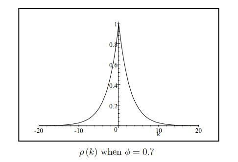
We have : Theorem 39 The autocorrelation function of a stationary AR(1) process is: $$ \rho(k)=\phi^{|k|} . $$ Proof. From Theorem 30 it follows that $$ \begin{aligned} \rho(k) & =\frac{\gamma(k)}{\gamma(0)} \ & =\frac{\phi^{|k|} \frac{\sigma^2}{1-\phi^2}}{\frac{\sigma^2}{1-\phi^2}} \ & =\phi^{|k|} . \end{aligned} $$
We plot $\rho(k)$ an $\operatorname{AR}(1)$ with $\phi=0.7$ below: ${ }^2$ $$ \rho(k) \text { when } \phi=0.7 $$ Since $|\phi|<1$ it follows that the autocorrelation function, like the autocovariance function, has the short-memory property so that $\rho(k)=O\left(\tau^k\right)$ as given in Section 2.2 with $A=1$ and $\tau=|\phi|$.
如果你也在 怎样代写时间序列Time Series 这个学科遇到相关的难题,请随时右上角联系我们的24/7代写客服。时间序列Time Series是在一段时间内以连续顺序出现的数据点序列。这可以与横截面数据进行对比,后者捕获一个时间点。在投资中,时间序列跟踪所选数据点(如证券价格)在指定时间段内的运动,并以固定的间隔记录数据点。没有必须包括的最小或最大时间,允许以一种方式收集数据,提供投资者或分析人员检查活动所寻求的信息。
统计代写|时间序列分析代写Time-Series Analysis代考|The Autocovariance Function
An important implication of stationarity is that the covariance between the business cycle in say the first and third quarters of say 1999 is the same as the covariance between the business cycle the first and third quarters of say 1963 . In general covariances only depend on the number of periods separating $Y_t$ and $Y_s$ so that:
Theorem 20 If $Y_t$ is stationary then $\operatorname{Cov}\left[Y_{t_1}, Y_{t_2}\right]$ depends only on $k=t_1-t_2$; that is the number of periods separating $t_1$ and $t_2$.
Since we will often be focusing on covariances, and since $\operatorname{Cov}\left[Y_t, Y_{t-k}\right]$ only depends on $k$, let us define this as a function of $k$ as: $\gamma(k)$, which we will refer to as the autocovariance function so that:
Definition 21 Autocovariance Function: Let $Y_t$ be a stationary time series with $E\left[Y_t\right]=0$. The autocovariance function for $Y_t$, denoted as $\gamma(k)$, is defined for $k=0, \pm 1, \pm 2, \pm 3, \ldots \pm \infty$ as: $$ \gamma(k) \equiv E\left[Y_t Y_{t-k}\right]=\operatorname{Cov}\left[Y_t, Y_{t-k}\right] . $$ We have the following results for the autocovariance function: Theorem $22 \gamma(0)=\operatorname{Var}\left[Y_t\right]>0$ Theorem $23 \gamma(k)=E\left[Y_t Y_{t-k}\right]=E\left[Y_s Y_{s-k}\right]$ for any $t$ and $s$. Theorem $24 \gamma(-k)=\gamma(k)(\gamma(k)$ is an even function $)$
统计代写|时间序列分析代写Time-Series Analysis代考|The AR(1) Model
For the AR(1) model we have already shown that: $$ \gamma(0)=\operatorname{Var}\left[Y_t\right]=\frac{\sigma^2}{1-\phi^2} $$ and that for $k>0$ : $$ \begin{aligned} \gamma(k) & =\phi^k \gamma(0) \ & =\phi^k \frac{\sigma^2}{1-\phi^2} . \end{aligned} $$ We can make this formula correct for all $k$ by appealing to Theorem 24 and replacing $k$ with $|k|$ to obtain:
Theorem 30 For an $A R(1)$ process the autocovariance function is given by: $$ \gamma(k)=\frac{\phi^{|k|} \sigma^2}{1-\phi^2} . $$
如果你也在 怎样代写时间序列Time Series 这个学科遇到相关的难题,请随时右上角联系我们的24/7代写客服。时间序列Time Series是在一段时间内以连续顺序出现的数据点序列。这可以与横截面数据进行对比,后者捕获一个时间点。在投资中,时间序列跟踪所选数据点(如证券价格)在指定时间段内的运动,并以固定的间隔记录数据点。没有必须包括的最小或最大时间,允许以一种方式收集数据,提供投资者或分析人员检查活动所寻求的信息。
Many of the models that we will be considering will have the property that they quickly forget or quickly become independent of what occurs either in the distant future or the distant past. This forgetting occurs at an exponential rate which represents a very rapid type of decay.
For example if you have a pie in the fridge and you eat one-half of the pie each day, you will quickly have almost no pie. After only ten days you would have: $$ \left(\frac{1}{2}\right)^{10}=\frac{1}{1024} $$ or about one-thousandth of a pie; maybe a couple of crumbs. We will see that for stationary $\operatorname{ARMA}(\mathrm{p}, \mathrm{q})$ processes, the infinite moving average weights: $\psi_k$, the autocorrelation function $\rho(k)$ and the forecast function $E_t\left[Y_{t+k}\right]$, all functions of the number of periods $k$, all have the short-memory property which we now define:
Definition 12 Short-Memory: Let $P_k$ for $k=0,1,2, \ldots \infty$ be some numerical property of a stationary time series which depends on $k$, the number of periods. We say $P_k$ displays a short-memory or $P_k=O\left(\tau^k\right)$ if $$ \left|P_k\right| \leq A \tau^k $$ where $A \geq 0$ and $0<\tau<1$.
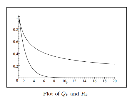
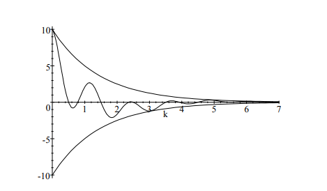
If $P_k=O\left(\tau^k\right)$ or if $P_k$ has a short-memory then $P_k$ decays rapidly in the same, manner that is at least as fast as $\tau^k$ decays to zero as $k \rightarrow \infty$. For example if: $$ P_k=10 \cos (2 k)\left(-\frac{1}{2}\right)^k $$ then $P_k$ decays rapidly in a manner which is bounded by exponential decay since $|\cos (2 k)| \leq 1$ and so we have: $$ \left|P_k\right| \leq 10\left(\frac{1}{2}\right)^k=A \tau^k $$ where $\tau=\frac{1}{2}$ and $A=10$. This is illustrated in the plot below: $$ P_k=10 \cos (2 k)\left(-\frac{1}{2}\right)^k $$ Not everything decays so rapidly. For example if we reverse the $\frac{1}{2}$ and the $k$ in $\left(\frac{1}{2}\right)^k$ we obtain: $$ Q_k=\frac{1}{k^{\frac{1}{2}}}=k^{-\frac{1}{2}} . $$
统计代写|时间序列分析代写Time-Series Analysis代考|The AR(1) Model
The simplest interesting model for $Y_t$ is a first-order autoregressive process or $\mathrm{AR}(1)$ which can be written as: $$ Y_t=\phi Y_{t-1}+a_t, a_t \sim \text { i.i.n }\left(0, \sigma^2\right), $$ where i.i.n. $\left(0, \sigma^2\right)$ means that $a_t$ is independently and identically distributed (i.i.d.) with a normal distribution with mean 0 and variance $\sigma^2$ so that the density of $a_t$ is: $$ p\left(a_t\right)=\frac{1}{\sqrt{2 \pi \sigma^2}} e^{-\frac{1}{2} a_t^2} . $$ We can attempt to calculate $E\left[Y_t\right]$ by taking expectations of both sides of (2.6) to obtain: $$ \begin{aligned} E\left[Y_t\right] & =\phi E\left[Y_{t-1}\right]+E\left[a_t\right] \ & =\phi E\left[Y_{t-1}\right] \end{aligned} $$ since $E\left[a_t\right]=0$. We now need to find $E\left[Y_{t-1}\right]$. We could try the same approach with $E\left[Y_{t-1}\right]$ since $Y_{t-1}=\phi Y_{t-2}+a_{t-1}$ from which we would conclude that: $E\left[Y_{t-1}\right]=\phi E\left[Y_{t-2}\right]$ so that: $$ E\left[Y_t\right]=\phi^2 E\left[Y_{t-2}\right] ; $$ but now we now need to find $E\left[Y_{t-2}\right]$. Clearly this process will never end. If, however, we assume stationarity then it is possible to break this infinite regress since by the definition of stationarity in Definition 7: $$ E\left[Y_t\right]=E\left[Y_{t-1}\right] . $$ It then follows from (2.8) that: $$ E\left[Y_t\right]=\phi E\left[Y_t\right] $$ or $$ (1-\phi) E\left[Y_t\right]=0 . $$
如果你也在 怎样代写时间序列Time Series 这个学科遇到相关的难题,请随时右上角联系我们的24/7代写客服。时间序列Time Series是在一段时间内以连续顺序出现的数据点序列。这可以与横截面数据进行对比,后者捕获一个时间点。在投资中,时间序列跟踪所选数据点(如证券价格)在指定时间段内的运动,并以固定的间隔记录数据点。没有必须包括的最小或最大时间,允许以一种方式收集数据,提供投资者或分析人员检查活动所寻求的信息。
The main disadvantage of the kernel smoothing method and the multitaper smoothing method is that they cannot guarantee that the final estimate is positive semidefinite while allowing flexible smoothing for each element of the spectral matrix. Thus, the same bandwidth is often applied to smoothing all the spectral components. However, in many applications, different components of the spectral matrix may need different smoothnesses, and require different smoothing parameters to get optimal estimates. To overcome this difficulty, Dai and Guo (2004) proposed a Cholesky decomposition based smoothing spline method for the spectrum estimation. The method models each Cholesky component separately by using different smoothing parameters. The method first obtains positive-definite and asymptotically unbiased initial spectral estimator $\widetilde{\mathbf{f}}_M(\omega)$ through sine multitapers as shown in Eq. (9.65). Then, it further smooths the Cholesky components of the spectral matrix via the smoothing spline and penalized sum of squares, which allows different degrees of smoothness for different Cholesky elements.
Suppose the spectral matrix $\tilde{\mathbf{f}}(\omega)$ has Cholesky decomposition such that $\tilde{\mathbf{f}}(\omega)=\mathbf{\Gamma} \mathbf{\Gamma}^*$, where $\boldsymbol{\Gamma}$ is $m \times m$ lower triangular matrix. To obtain unique decomposition, the diagonal elements of $\boldsymbol{\Gamma}$ are constrained to be positive. The diagonal elements $\gamma_{j, j}, j=1, \ldots, m$, the real part of $\gamma_{j, k}, \Re\left(\gamma_{j, k}\right)$, and imaginary part of $\gamma_{j, k}, \mathfrak{\Im}\left(\gamma_{j, k}\right), j>k$ are smoothed by spline with different smoothing parameters. Suppose $\gamma \in\left{\gamma_{j, j}, \Re\left(\gamma_{j, k}\right), \mathfrak{\Im}\left(\gamma_{j, k}\right), j>k\right.$, for $\left.j, k=1, \ldots, m\right}$, we have $$ \gamma\left(\omega_{\ell}\right)=a\left(\omega_{\ell}\right)+e\left(\omega_{\ell}\right), $$ where $a\left(\omega_{\ell}\right)=\mathrm{E}\left{\gamma\left(\omega_{\ell}\right)\right}$, and the $e\left(\omega_{\ell}\right), \ell=1, \ldots, n$, are independent errors with zero means and the variances depending on the frequency point $\omega_{\ell} \cdot a(\cdot)$ is periodic and is fitted by periodic smoothing spline (Wahba, 1990) of the form, $$ a(\omega)=c_0+\sum_{\nu=1}^{n / 2-1} c_\nu \sqrt{2} \cos (2 \pi \nu \omega)+\sum_{\nu=1}^{n / 2-1} d_\nu \sqrt{2} \sin (2 \pi \nu \omega)+c_{n / 2} \cos (\pi n \omega) $$
Penalized methods have been one of the most popular research topics for the past decade. In the area of spectrum estimation, Pawitan and O’Sullivan (1994) developed penalized likelihood method for the nonparametric estimation of the power spectrum of a univariate time series. Pawitan (1996) developed a penalized Whittle likelihood estimator for a bivariate time series. However, their approach cannot be easily generalized to higher dimension. More recently, Krafty and Collinge (2013) proposed a penalized Whittle likelihood method to estimate the power spectrum of a vector-valued time series. The method allows for varying levels of smoothness among spectral components while accounting for the positive definiteness of spectral matrices and the Hermitian and periodic structures of power spectra as functions of frequency. In this section, we briefly discuss the method by Krafty and Collinge (2013). Recall that $\widetilde{\mathbf{Y}}{\ell}=\widetilde{\mathbf{Y}}\left(\omega{\ell}\right)$ are discrete Fourier transform of the time series, and define the negative log Whittle likelihood as $$ L(\mathbf{f})=\sum_{\ell=1}^L\left{\log \left|\mathbf{f}\left(\omega_{\ell}\right)\right|+\widetilde{\mathbf{Y}}{\ell}^\left[\mathbf{f}\left(\omega{\ell}\right)\right]^{-1} \widetilde{\mathbf{Y}}{\ell}\right}, $$ where $\omega{\ell}=\ell / n$ and $L=[(n-1) / 2]$. Based on $L$, the method penalizes the roughness of the estimated spectrum. The spectral matrix $\mathbf{f}(\omega)$ is modeled by the Cholesky decomposition such that $\mathbf{f}(\omega)=\left[\mathbf{\Gamma} \boldsymbol{\Gamma}^\right]^{-1}$, where $\boldsymbol{\Gamma}$ is a $m \times m$ lower triangular matrix with real-valued diagonal elements. Further, denote $\boldsymbol{\Gamma}{i, j, R}(\omega ; \mathbf{f})$ and $\boldsymbol{\Gamma}{i, j, l}(\omega ; \mathbf{f})$ as the real and imaginary parts of the $(i, j)$ element of $\boldsymbol{\Gamma}$. The method proposes a measure of roughness of a power spectrum through the integrated squared $k$ th derivatives of the $m(m+1) / 2$ real and $m(m-1) / 2$ imaginary components of the Cholesky decomposition. Suppose the smoothing parameters, $\lambda=\left{\rho_{i, j}\right.$, $\left.\theta_{i, j}: i \leq j=1, \ldots, m\right}$, of $\boldsymbol{\Gamma}{i, j, R}$ and $\boldsymbol{\Gamma}{i, j, I}$ that control the roughness penalty are $\rho_{i, j}>0$ and $\theta_{i, j}$ $>0$, the roughness measure for a spectrum $\tilde{\mathbf{f}}(\omega)$ is $$ J_\lambda(\mathbf{f})=\sum_{i \leq j=1}^m \rho_{i, j} \int_0^{1 / 2}\left{\boldsymbol{\Gamma}{i, j, R}^{(k)}(\omega ; \mathbf{f})\right}^2 d \omega+\sum{i<j=1}^m \theta_{i, j} \int_0^{1 / 2}\left{\boldsymbol{\Gamma}{i, j, I}^{(k)}(\omega ; \mathbf{f})\right}^2 d \omega . $$ The interpretation is that the penalty function $J$ shrinks the estimates of power spectra toward real-valued matrix functions that are constant across frequency. Consequently, we consider minimizing the penalized Whittle negative loglikelihood $$ Q\lambda(\mathbf{f})=L(\mathbf{f})+J_\lambda(\mathbf{f}) . $$
如果你也在 怎样代写时间序列Time Series 这个学科遇到相关的难题,请随时右上角联系我们的24/7代写客服。时间序列Time Series是在一段时间内以连续顺序出现的数据点序列。这可以与横截面数据进行对比,后者捕获一个时间点。在投资中,时间序列跟踪所选数据点(如证券价格)在指定时间段内的运动,并以固定的间隔记录数据点。没有必须包括的最小或最大时间,允许以一种方式收集数据,提供投资者或分析人员检查活动所寻求的信息。
统计代写|时间序列分析代写Time-Series Analysis代考|Parameter estimation, diagnostic checking, and forecasting
Given a vector time series of $n$ observations, $\mathbf{Z}t, t=1,2, \ldots, n$, once a tentative VARMA $(p, q)$ model is identified, $$ \mathbf{Z}_t-\boldsymbol{\Phi}_1 \mathbf{Z}{t-1}-\cdots-\boldsymbol{\Phi}p \mathbf{Z}{t-p}=\boldsymbol{\theta}0+\mathbf{a}_t-\boldsymbol{\Theta}_1 \mathbf{a}{t-1}-\cdots-\boldsymbol{\Theta}q \mathbf{a}{t-q} $$ The efficient estimates of the parameters, $\boldsymbol{\Phi}=\left(\boldsymbol{\Phi}1, \ldots, \boldsymbol{\Phi}_p\right), \boldsymbol{\theta}_0, \boldsymbol{\Theta}=\left(\boldsymbol{\Theta}_1, \ldots, \boldsymbol{\Theta}_q\right)$, and $\boldsymbol{\Sigma}$, are obtained by using a maximum likelihood method. Specifically, assuming the vector white noise is Gaussian, the log-likelihood function is given by $$ \begin{aligned} \ln L\left(\boldsymbol{\Phi}, \boldsymbol{\theta}_0, \boldsymbol{\Theta}, \boldsymbol{\Sigma} \mid \mathbf{Z}\right) & =-\frac{n m}{2} \ln 2 \pi-\frac{n}{2}|\mathbf{\Sigma}|-\frac{1}{2} \sum{t=1}^n \mathbf{a}_t^{\prime} \mathbf{\Sigma}^{-\mathbf{1}} \mathbf{a}_t \ & =-\frac{n m}{2} \ln 2 \pi-\frac{n}{2}|\mathbf{\Sigma}|-\frac{1}{2} \operatorname{tr} \boldsymbol{\Sigma}^{-1} S\left(\boldsymbol{\Phi}, \boldsymbol{\theta}_0, \boldsymbol{\Theta}\right), \end{aligned} $$
where $$ \mathbf{a}t=\mathbf{Z}_t-\boldsymbol{\Phi}_1 \mathbf{Z}{t-1}-\cdots-\boldsymbol{\Phi}p \mathbf{Z}{t-p}-\boldsymbol{\theta}0+\boldsymbol{\Theta}_1 \mathbf{a}{t-1}+\cdots+\boldsymbol{\Theta}q \mathbf{a}{t-q}, $$ and $$ S\left(\boldsymbol{\Phi}, \boldsymbol{\theta}0, \boldsymbol{\Theta}\right)=\sum{t=1}^n \mathbf{a}_t \mathbf{a}_t^{\prime} . $$ The computation method is available in many statistical packages such as EViews (2016), MATLAB (2017), R (2009), SAS (2015), SCA (2008), and SPSS (2009).
After the parameters are estimated, it is important to check the adequacy of the model through a careful analysis of the residuals $$ \hat{\mathbf{a}}t=\mathbf{Z}_t-\hat{\boldsymbol{\Phi}}_1 \mathbf{Z}{t-1}-\cdots-\hat{\boldsymbol{\Phi}}p \mathbf{Z}{t-p}-\hat{\boldsymbol{\theta}}0+\hat{\boldsymbol{\Theta}}_1 \hat{\mathbf{a}}{t-1}+\cdots+\hat{\boldsymbol{\Theta}}q \hat{\mathbf{a}}{t-q} . $$
统计代写|时间序列分析代写Time-Series Analysis代考|Seasonal vector time series model
The VARMA $(p, q)$ model in Eq. (2.42) can be extended to a seasonal vector model that contains both seasonal and non-seasonal AR and MA polynomials as follows, $$ \boldsymbol{\alpha}P\left(B^s\right) \boldsymbol{\Phi}_p(B) \mathbf{Z}_t=\boldsymbol{\theta}_0+\boldsymbol{\beta}_Q\left(B^s\right) \boldsymbol{\Theta}_q(B) \mathbf{a}_t, $$ where $$ \begin{aligned} & \boldsymbol{\alpha}_P\left(B^s\right)=\mathbf{I}-\boldsymbol{\alpha}_1 B^s-\cdots-\boldsymbol{\alpha}_P B^{P s}=\mathbf{I}-\sum{k=1}^P \boldsymbol{\alpha}k B^{k s}, \ & \boldsymbol{\beta}_Q\left(B^s\right)=\mathbf{I}-\boldsymbol{\beta}_1 B^s-\cdots-\boldsymbol{\beta}_Q B^{Q s}=\mathbf{I}-\sum{k=1}^Q \boldsymbol{\beta}_k B^{k s}, \end{aligned} $$ and $s$ is a seasonal period. $\boldsymbol{\alpha}_k$ and $\boldsymbol{\beta}_k$ are seasonal AR and seasonal MA parameters, respectively. $P$ is the seasonal AR order, $Q$ is the seasonal MA order. The zeros of $\left|\boldsymbol{\alpha}_P(B)\right|$ and $\left|\boldsymbol{\beta}_Q(B)\right|$ are outside of the unit circle. For simplicity, we will denote the seasonal vector time series model in Eq. (2.78) with a seasonal period $s$ as $\operatorname{VARMA}(p, q) \times(P, Q)_s$.
It is important to point out that for a univariate time series, the polynomials in Eq. (2.78) are scalar and they are commutative. For example, for a univariate seasonal AR model, the two representations, $$ \alpha_P\left(B^s\right) \phi_p(B) Z_t=a_t \text {, and } \phi_p(B) \alpha_P\left(B^s\right) Z_t=a_t, $$ are exactly the same. However, for a vector seasonal VAR model, the two representations, $$ \boldsymbol{\alpha}_P\left(B^s\right) \boldsymbol{\Phi}_p(B) \mathbf{Z}_t=\mathbf{a}_t \text {, and } \boldsymbol{\Phi}_p(B) \boldsymbol{\alpha}_P\left(B^s\right) \mathbf{Z}_t=\mathbf{a}_t, $$ are not the same, because the vector multiplications are not commutative. This leads to many complications in terms of model identification, parameter estimation, and forecasting. We refer readers to an interesting and excellent paper by Yozgatligil and Wei (2009) for more details and examples.
如果你也在 怎样代写时间序列Time Series 这个学科遇到相关的难题,请随时右上角联系我们的24/7代写客服。时间序列Time Series是在一段时间内以连续顺序出现的数据点序列。这可以与横截面数据进行对比,后者捕获一个时间点。在投资中,时间序列跟踪所选数据点(如证券价格)在指定时间段内的运动,并以固定的间隔记录数据点。没有必须包括的最小或最大时间,允许以一种方式收集数据,提供投资者或分析人员检查活动所寻求的信息。
The $m$-dimensional vector autoregressive process or model of order $p$, shortened to VAR $(p)$, is given by $$ \mathbf{Z}t=\boldsymbol{\theta}_0+\boldsymbol{\Phi}_1 \mathbf{Z}{t-1}+\cdots+\boldsymbol{\Phi}p \mathbf{Z}{t-p}+\mathbf{a}_t $$ or $$ \boldsymbol{\Phi}_p(B) \mathbf{Z}_t=\boldsymbol{\theta}_0+\mathbf{a}_t, $$ where $\mathbf{a}_t$ is a sequence of $m$-dimensional vector white noise process, $\operatorname{VWN}(\mathbf{0}, \boldsymbol{\Sigma})$, and $$ \boldsymbol{\Phi}_p(B)=\mathbf{I}-\boldsymbol{\Phi}_1 B-\cdots-\boldsymbol{\Phi}_p B^p . $$
The model is clearly invertible. It will be stationary if the zeros of $\left|\mathbf{I}-\boldsymbol{\Phi}1 B-\cdots-\boldsymbol{\Phi}_p B^p\right|$ lie outside of the unit circle or equivalently, the roots of $$ \left|\lambda^p \mathbf{I}-\lambda^{p-1} \boldsymbol{\Phi}_1-\cdots-\boldsymbol{\Phi}_p\right|=0 $$ are all inside the unit circle. In this case, its mean is a constant vector, $E\left(\mathbf{Z}_t\right)=\boldsymbol{\mu}$, which can be found by noting that $$ \begin{aligned} \boldsymbol{\mu} & =E\left(\mathbf{Z}_t\right)=E\left(\boldsymbol{\theta}_0+\boldsymbol{\Phi}_1 \mathbf{Z}{t-1}+\cdots+\boldsymbol{\Phi}p \mathbf{Z}{t-p}+\mathbf{a}_t\right) \ & =\boldsymbol{\theta}_0+\boldsymbol{\Phi}_1 \boldsymbol{\mu}+\cdots+\boldsymbol{\Phi}_p \boldsymbol{\mu} \end{aligned} $$ and hence $$ \boldsymbol{\mu}=\left(\mathbf{I}-\boldsymbol{\Phi}_1-\cdots-\boldsymbol{\Phi}_p\right)^{-1} \boldsymbol{\theta}_0 . $$ Since $$ \boldsymbol{\theta}_0=\left(\mathbf{I}-\boldsymbol{\Phi}_1-\cdots-\boldsymbol{\Phi}_p\right) \boldsymbol{\mu}=\left(\mathbf{I}-\boldsymbol{\Phi}_1 B-\cdots-\boldsymbol{\Phi}_p B^p\right) \boldsymbol{\mu}, $$
Equation (2.18) can be written as $$ \boldsymbol{\Phi}p(B) \dot{\mathbf{Z}}_t=\mathbf{a}_t, $$ or $$ \dot{\mathbf{Z}}_t=\boldsymbol{\Phi}_1 \dot{\mathbf{Z}}{t-1}+\cdots+\boldsymbol{\Phi}p \dot{\mathbf{Z}}{t-p}+\mathbf{a}_t, $$ where $\dot{\boldsymbol{Z}}_t=\boldsymbol{Z}_t-\boldsymbol{\mu}$.
One of the interesting problems in studying a vector time series is that we often want to know whether there are any causal effects among these variables. Specifically, in a VAR $(p)$ model $$ \boldsymbol{\Phi}p(B) \mathbf{Z}_t=\boldsymbol{\theta}_0+\mathbf{a}_t, $$ we can partition the vector $\mathbf{Z}_t$ into two components, $\mathbf{Z}_t=\left[\mathbf{Z}{1, t}^{\prime}, \mathbf{Z}{2, t}^{\prime}\right]^{\prime}$ so that $$ \left[\begin{array}{ll} \boldsymbol{\Phi}{11}(B) & \boldsymbol{\Phi}{12}(B) \ \boldsymbol{\Phi}{21}(B) & \boldsymbol{\Phi}{22}(B) \end{array}\right]\left[\begin{array}{l} \mathbf{Z}{1, t} \ \mathbf{Z}{2, t} \end{array}\right]=\left[\begin{array}{l} \boldsymbol{\theta}_1 \ \boldsymbol{\theta}_2 \end{array}\right]+\left[\begin{array}{l} \mathbf{a}{1, t} \ \mathbf{a}{2, t} \end{array}\right] $$ When $\boldsymbol{\Phi}{12}(B)=\mathbf{0}$, Eq. (2.40) becomes $$ \left{\begin{array}{l} \boldsymbol{\Phi}{11}(B) \mathbf{Z}{1, t}=\boldsymbol{\theta}1+\mathbf{a}{1, t} \ \boldsymbol{\Phi}{22}(B) \mathbf{Z}{2, t}=\boldsymbol{\theta}2+\boldsymbol{\Phi}{21}(B) \mathbf{Z}{1, t}+\mathbf{a}{2, t} \end{array}\right. $$ The future values of $\mathbf{Z}{2, t}$ are influenced not only by its own past but also by the past of $\mathbf{Z}{1, t}$, while the future values of $\mathbf{Z}{1, t}$ are influenced only by its own past. In other words, we say that variables in $\mathbf{Z}{1, t}$ cause $\mathbf{Z}{2, t}$, but variables in $\mathbf{Z}{2, t}$ do not cause $\mathbf{Z}_{1, t}$. This concept is often known as the Granger causality, because it is thought to have been Granger who first introduced the notion in 1969. For more discussion about causality and its tests, we refer readers to Granger (1969), Hawkes (1971a, b), Pierce and Haugh (1977), Eichler et al. (2017), and Zhang and Yang (2017), among others.
统计代写|时间序列分析代写Time-Series Analysis代考|The space–time AR (STAR) model
统计代写|时间序列分析代写Time-Series Analysis代考|The space–time AR (STAR) model
Similar to the regularization methods that control the values of parameters, when modeling time series associated with spaces or locations, it is very likely that many elements of $\boldsymbol{\Phi}k$ are not significantly different from zero for pairs of locations that are spatially far away and uncorrelated given information from other locations. Thus, a model incorporating spatial information is not only helpful for parameter estimation, but also for dimension reduction and forecasting. For a zero-mean stationary spatial time series, the space-time autoregressive moving average STARMA $\left(p{a_1, \ldots, a_p}, q_{m_1, \ldots, m_q}\right)$ model is defined by $$ \mathbf{Z}t=\sum{k=1}^p \sum_{\ell=0}^{a_k} \phi_{k, \ell} \mathbf{W}^{(\ell)} \mathbf{Z}{t-k}+\mathbf{a}_t-\sum{k=1}^q \sum_{\ell=0}^{m_k} \theta_{k, \ell} \mathbf{W}^{(\ell)} \mathbf{a}{t-k}, $$ where the zeros of $\operatorname{det}\left(\mathbf{I}-\sum{k=1}^p \sum_{\ell=0}^{a_k} \phi_{k, \ell} \mathbf{W}^{(\ell)} B^k\right)=0$ lie outside the unit circle, $\mathbf{a}t$ is a Gaussian vector white noise process with zero-mean vector $\mathbf{0}$, and covariance matrix structure $$ E\left[\mathbf{a}_t \mathbf{a}{t+k}^{\prime}\right]=\left{\begin{array}{l} \boldsymbol{\varepsilon}, \text { if } k=0, \ \mathbf{0}, \text { if } k \neq 0, \end{array}\right. $$ and $\boldsymbol{\varepsilon}$ is an $m \times m$ symmetric positive definite matrix. The STARMA $\left(p_{a_1, \ldots, a_p}, q_{m_1, \ldots, m_q}\right)$ model becomes a space-time autoregressive $\operatorname{STAR}\left(p_{a_1, \ldots, a_p}\right)$ model when $q=0$. The STAR models were first introduced by Cliff and Ord (1975) and further extended to STARMA models by Pfeifer and Deutsch (1980a, b, c). Since a stationary model can be approximated by an autoregressive model, because of its easier interpretation, the most widely used STARMA models in practice are $\operatorname{STAR}\left(p_{a_1, \ldots, a_p}\right)$ models, $$ \mathbf{Z}t=\sum{k=1}^p \sum_{\ell=0}^{a_k} \phi_{k, \ell} \mathbf{W}^{(\ell)} \mathbf{Z}_{t-k}+\mathbf{a}_t, $$ where $\mathbf{Z}_t$ is a zero-mean stationary spatial time series or a proper differenced and transformed series of a nonstationary spatial time series.
Clustering or cluster analysis is a methodology that has been used by researchers to group data into homogeneous groups for a long time and may have originated in the fields of anthropology and psychology. There are many methods of clustering, including subjective observation and various distance methods for similarity. Earlier works include Tryon (1939), Cattell (1943), Ward (1963), Macqueen (1967), McLachlan and Basford (1988), among others. We will discuss these further in the last section. These methods were extended to the model-based cluster approach with an associated probability distribution by researchers including Banfield and Raftery (1993), Fraley and Raftery (2002), Wang and Zhou (2008), Scrucca (2010), and others. More recently, Wang et al. (2013) introduced a robust model-based clustering method for forecasting high-dimensional time series, and in this section, we will use their approach as an illustration. Let $p_h$ be the probability a time series belongs to cluster $h$. The method first groups multiple time series into $H$ mutually exclusive clusters, $\sum_{h=1}^H p_h=1$, and assumes that each mean adjusted time series in a given cluster follows the same $\operatorname{AR}(p)$ model. Thus, for the $i$ th time series that is in cluster $h$, we have, $$ Z_{i, t}=\sum_{k=1}^p \phi_k^{(h)} Z_{i, t-k}+\sigma_h \varepsilon_{i, t}, \text { for } t=p+1, \ldots, n, $$ where $h=1,2, \ldots, H$, the $\varepsilon_{i, t}$ are $i . i . d . N(0,1)$ random variables, independent across time and series. Let $\boldsymbol{\theta}_h=\left(\phi_1^{(h)}, \phi_2^{(h)}, \ldots, \phi_p^{(h)}, \sigma^{(h)}\right)$ be the vector of all parameters in cluster $h$, and $\boldsymbol{\Theta}=$ $\left(\boldsymbol{\theta}_1, \ldots, \boldsymbol{\theta}_H, \boldsymbol{\eta}\right)$, where $\boldsymbol{\eta}=\left(p_1, \ldots, p_H\right)$. The estimation procedure is accomplished through the Bayesian Markov Chain and Monte Carlo method.
统计代写|时间序列分析代写Time-Series Analysis代考|The space–time AR (STAR) model
统计代写|时间序列分析代写Time-Series Analysis代考|Time-varying autoregressive model
统计代写|时间序列分析代写Time-Series Analysis代考|Time-varying autoregressive model
One of the methods used in Dahlhaus (2000) is the time-varying VARMA $(p, q)$ model. For a vector autoregressive model $\operatorname{VAR}(p)$, it is defined by $$ \mathbf{Z}t=\boldsymbol{\mu}(t / n)+\sum{j=1}^p \boldsymbol{\Phi}j(t / n)\left[\mathbf{Z}{t-j}-\boldsymbol{\mu}[(t-j)]+\boldsymbol{\Sigma}(t / n) \boldsymbol{\varepsilon}t, t=1, \ldots, n,\right. $$ where $\boldsymbol{\varepsilon}_t$ are $m$-dimensional independent random variable with mean zero and unit variance $\mathbf{I}$. In addition, we assume some smoothness conditions on $\boldsymbol{\Sigma}(\cdot)$ and $\boldsymbol{\Phi}_j(\cdot)$. In some neighborhood of a fixed time point $u_0=t_0 / n$, the process $\mathbf{Z}_t$ can be approximated by the stationary process $\mathbf{Z}_t\left(u_0\right)$ given by $$ \mathbf{Z}_t\left(u_0\right)=\boldsymbol{\mu}\left(u_0\right)+\sum{j=1}^p \boldsymbol{\Phi}j\left(u_0\right)\left[\mathbf{Z}{t-j}\left(u_0\right)-\boldsymbol{\mu}\left(u_0\right)+\boldsymbol{\Sigma}\left(u_0\right) \boldsymbol{\varepsilon}_t, t=1, \ldots, n .\right. $$ $\mathbf{Z}_t$ has a unique time-varying power spectrum, which is locally the same as the power spectrum of $\mathbf{Z}_t(u)$, that is, $$ \mathbf{f}(u, \omega)=\left[\boldsymbol{\Phi}\left(u, e^{-i \omega}\right)\right]^{-1} \boldsymbol{\Sigma}(u)\left{\left[\boldsymbol{\Phi}\left(u, e^{-i \omega}\right)\right]^{-1}\right}^*, $$
where $u=t / n$, and $$ \boldsymbol{\Phi}(u, B)=\left(\mathbf{I}-\boldsymbol{\Phi}1(u, B)-\cdots-\boldsymbol{\Phi}_p\left(u, B^p\right)\right) . $$ Similarly, the locally covariance matrix is $$ \boldsymbol{\Gamma}(u, j)=\int{-\pi}^\pi \mathbf{f}(u, \omega) \exp (j i \omega) d \omega . $$ Based on this statement, the time-varying spectrum can be obtained by estimating the timevarying parameters of the VAR model. For more properties of the estimation based on timevarying VARMA $(p, q), \operatorname{VAR}(p)$, and $\operatorname{VMA}(q)$ models, we refer readers to Dahlhaus (2000).
统计代写|时间序列分析代写Time-Series Analysis代考|Smoothing spline ANOVA model
Based on the locally stationary process, the time-varying spectrum can also be estimated nonparametrically via the smoothing spline Analysis of Variance (ANOVA) model by Guo and Dai (2006). However, their definition of locally stationary process is slightly different from Dahlhaus (2000). In Section 9.5.2, we mentioned that Dahlhaus (2000) assumes a series of transfer functions $\mathbf{A}^0(t / n, \omega)$ that converge to a large-sample transfer function $\mathbf{A}(u, \omega)$ in order to allow for the fitting of parametric models. Since Guo and Dai (2006) considered a nonparametric estimation, they used $\mathbf{A}(u, \omega)$ directly.
Definition 9.2 Without loss of generality, the $m$-dimensional zero-mean time series of length $n,\left{\mathbf{Z}t: t=1, \ldots, n\right}$, is called locally stationary if $$ \mathbf{Z}_t=\int{-\pi}^\pi \mathbf{A}(t / n, \omega) \exp (i \omega t) d \mathbf{U}(\omega), $$ where we assume that the cumulants of $d \mathbf{U}(\omega)$ exists and are bounded for all orders. For the details, please see Brillinger (2002), and Guo and Dai (2006).
Based on this definition, the smoothing ANOVA model takes a two-stage estimation procedure. At the first stage, the locally stationary process is approximated by piecewise stationary time series with small blocks to obtain initial spectrum estimates and the Cholesky decomposition. The initial spectrum estimates are obtained by the multitaper method to reduce variance. At the second stage, each element of the Cholesky decomposition is treated as a bivariate smooth function of time and frequency and is modeled by the smoothing spline ANOVA model by Gu and Wahba (1993). The final estimated time-varying spectrum is reconstructed from the smoothed elements of the Cholesky decomposition. Thus, the method provides a way to ensure the final estimate of the multivariate spectrum is positive-definite while allowing enough flexibility in the smoothness of its elements.
We shall briefly discuss the smoothing spline ANOVA step. Suppose the spectral matrix $\widetilde{\mathbf{f}}(u, \omega)$ has the Cholesky decomposition such that $\widetilde{\mathbf{f}}(u, \omega)=\mathbf{L}(u, \omega) \mathbf{L}(u, \omega)^*$, where $\mathbf{L}(u, \omega)$ is a $m \times m$ lower triangular matrix. The method smooths the diagonal elements $\gamma_{j, j}(u, \omega), j=1, \ldots, m$, the real part of $\gamma_{j, k}(u, \omega), \mathfrak{R}\left{\gamma_{j, k}(u, \omega)\right}$, and the imaginary part of $\gamma_{j, k}(u, \omega), \mathfrak{J}\left{\gamma_{j, k}(u, \omega)\right}$, for $j>k$ separately with their own smoothing parameters. Let $\gamma(u, \omega) \in\left{\gamma_{j, j}(u, \omega), \mathfrak{R}\left(\gamma_{j, k}\right)(u, \omega), \mathfrak{\Im}\left(\gamma_{j, k}\right)\right.$ $(u, \omega), j>k$, for $j, k=1, \ldots, m}$. We have $$ \gamma(u, \omega)=a(u, \omega)+\varepsilon(u, \omega), $$where $a(u, \omega)$ is the corresponding Cholesky decomposition element of the spectrum, such that $a(u, \omega)=E{\gamma(u, \omega)}$, the $\varepsilon(u, \omega)$ are independent errors with zero-mean and the variance depending on the time-frequency point $(u, \omega)$.
统计代写|时间序列分析代写Time-Series Analysis代考|Time-varying autoregressive model
统计代写|时间序列分析代写Time-Series Analysis代考|Smoothing spline ANOVA model
基于局部平稳过程,还可以通过Guo和Dai(2006)的平滑样条方差分析(ANOVA)模型非参数地估计时变谱。然而,他们对局部平稳过程的定义与Dahlhaus(2000)略有不同。在第9.5.2节中,我们提到Dahlhaus(2000)假设一系列传递函数$\mathbf{A}^0(t / n, \omega)$收敛于一个大样本传递函数$\mathbf{A}(u, \omega)$,以便允许参数模型的拟合。由于Guo和Dai(2006)考虑了非参数估计,他们直接使用$\mathbf{A}(u, \omega)$。
定义9.2在不丧失一般性的前提下,长度为$n,\left{\mathbf{Z}t: t=1, \ldots, n\right}$的$m$维零平均时间序列,如果$$ \mathbf{Z}_t=\int{-\pi}^\pi \mathbf{A}(t / n, \omega) \exp (i \omega t) d \mathbf{U}(\omega), $$,则称为局部平稳 其中我们假设$d \mathbf{U}(\omega)$的累积量存在并且对所有阶都有界。详情请参见Brillinger(2002)和Guo and Dai(2006)。
The main disadvantage of the kernel smoothing method and the multitaper smoothing method is that they cannot guarantee that the final estimate is positive semidefinite while allowing flexible smoothing for each element of the spectral matrix. Thus, the same bandwidth is often applied to smoothing all the spectral components. However, in many applications, different components of the spectral matrix may need different smoothnesses, and require different smoothing parameters to get optimal estimates. To overcome this difficulty, Dai and Guo (2004) proposed a Cholesky decomposition based smoothing spline method for the spectrum estimation. The method models each Cholesky component separately by using different smoothing parameters. The method first obtains positive-definite and asymptotically unbiased initial spectral estimator $\widetilde{\mathbf{f}}_M(\omega)$ through sine multitapers as shown in Eq. (9.65). Then, it further smooths the Cholesky components of the spectral matrix via the smoothing spline and penalized sum of squares, which allows different degrees of smoothness for different Cholesky elements.
Suppose the spectral matrix $\tilde{\mathbf{f}}(\omega)$ has Cholesky decomposition such that $\widetilde{\mathbf{f}}(\omega)=\boldsymbol{\Gamma}^*$, where $\boldsymbol{\Gamma}$ is $m \times m$ lower triangular matrix. To obtain unique decomposition, the diagonal elements of $\boldsymbol{\Gamma}$ are constrained to be positive. The diagonal elements $\gamma_{j, j}, j=1, \ldots, m$, the real part of $\gamma_{j, k}, \mathfrak{R}\left(\gamma_{j, k}\right)$, and imaginary part of $\gamma_{j, k}, \mathfrak{T}\left(\gamma_{j, k}\right), j>k$ are smoothed by spline with different smoothing parameters. Suppose $\gamma \in\left{\gamma_{j, j}, \mathfrak{R}\left(\gamma_{j, k}\right), \mathfrak{\Im}\left(\gamma_{j, k}\right), j>k\right.$, for $\left.j, k=1, \ldots, m\right}$, we have $$ \gamma\left(\omega_{\ell}\right)=a\left(\omega_{\ell}\right)+e\left(\omega_{\ell}\right) $$ where $a\left(\omega_{\ell}\right)=\mathrm{E}\left{\gamma\left(\omega_{\ell}\right)\right}$, and the $e\left(\omega_{\ell}\right), \ell=1, \ldots, n$, are independent errors with zero means and the variances depending on the frequency point $\omega_{\ell} . a(\cdot)$ is periodic and is fitted by periodic smoothing spline (Wahba, 1990) of the form, $$ a(\omega)=c_0+\sum_{\nu=1}^{n / 2-1} c_\nu \sqrt{2} \cos (2 \pi \nu \omega)+\sum_{\nu=1}^{n / 2-1} d_\nu \sqrt{2} \sin (2 \pi \nu \omega)+c_{n / 2} \cos (\pi n \omega) $$
Recall that the discrete Fourier transform $\widetilde{\mathbf{Y}}{\ell}=\widetilde{\mathbf{Y}}\left(\omega{\ell}\right), \ell=0, \ldots,(n-1) / 2$, are approximately independent complex multivariate normal random variables. The large-sample distribution of $\widetilde{\mathbf{Y}}{\ell}$ leads to the Whittle likelihood (Whittle, 1953, 1954), $$ L(\mathbf{f})=\prod{\ell=1}^L\left|\mathbf{f}\left(\omega_{\ell}\right)\right|^{-1} \exp \left{-\widetilde{\mathbf{Y}}{\ell}^\left[\mathbf{f}\left(\omega{\ell}\right)\right]^{-1} \widetilde{\mathbf{Y}}{\ell}\right}, $$ where $\omega_k=\ell / n$ and $L=[(n-1) / 2]$. Based on the Whittle likelihood, Rosen and Stoffer (2007) proposed a Bayesian method to the estimate spectrum of the second-order stationary multivariate time series. They model the spectrum $\mathbf{f}(\omega)$ by the modified complex Cholesky factorization, such that, $$ \mathbf{f}^{-1}\left(\omega{\ell}\right)=\mathbf{\Gamma}{\ell}^ \mathbf{D}{\ell}^{-1} \mathbf{\Gamma}{\ell}, $$ where $\boldsymbol{\Gamma}{\ell}$ is a complex-valued lower triangular matrix with one on its diagonal, $$ \boldsymbol{\Gamma}{\ell}=\left[\begin{array}{ccccccc} 1 & 0 & \cdots & \cdots & \cdots & \cdots & 0 \ -\theta{2,1}^{(\ell)} & 1 & 0 & \cdots & \cdots & \cdots & 0 \ -\theta_{3,1}^{(\ell)} & -\theta_{3,2}^{(\ell)} & 1 & 0 & \cdots & \cdots & \vdots \ \vdots & \cdots & \vdots & \ddots & \ddots & \vdots & \vdots \ \vdots & \vdots & \vdots & \cdots & \ddots & 0 & \vdots \ \vdots & \cdots & \cdots & \cdots & \cdots & 1 & 0 \ -\theta_{m, 1}^{(\ell)} & -\theta_{m, 2}^{(\ell)} & \cdots & \cdots & \cdots & -\theta_{m, m-1}^{(\ell)} & 1 \end{array}\right], $$
and $\mathbf{D}{\ell}$ is a diagonal matrix with positive real values, that is, $\mathbf{D}{\ell}=\operatorname{diag}\left(d_{1, \ell}^2, \ldots, d_{m, \ell}^2\right)$. Let $\boldsymbol{\theta}{\ell}=\left(\theta{2,1}^{(\ell)}, \theta_{3,1}^{(\ell)}, \theta_{3,2}^{(\ell)}, \ldots, \theta_{m, m-1}^{(\ell)}\right), \boldsymbol{\Theta}=\left(\boldsymbol{\theta}1, \ldots, \boldsymbol{\theta}_L\right)$, and $\mathbf{D}=\left{\mathbf{D}_1, \ldots, \mathbf{D}_L\right}$, the modified Cholesky representation facilitates development of Bayesian sampler by noticing that the Whittle likelihood can be rewritten as $$ L(\mathbf{Y} \mid \mathbf{D}, \boldsymbol{\Theta}) \approx \prod{\ell=1}^L \prod_{j=1}^m d_{j, \ell}^{-2} \exp \left{-\left(\widetilde{\mathbf{Y}}\left(\omega_{\ell}\right)-\mathbf{R}{\ell} \boldsymbol{\theta}{\ell}\right)^* \mathbf{D}{\ell}^{-1}\left(\widetilde{\mathbf{Y}}\left(\omega{\ell}\right)-\mathbf{R}{\ell} \boldsymbol{\theta}{\ell}\right)\right}, $$ where $\boldsymbol{\theta}{\ell}$ is an $m(m-1) / 2$-dimensional vector and $\mathbf{R}{\ell}$ is a $m \times m(m-1) / 2$ design matrix such that
$$ \mathbf{R}{\ell}=\left[\begin{array}{ccccccccccccc} 0 & 0 & 0 & 0 & 0 & 0 & 0 & \ldots & 0 & 0 & 0 & \ldots & 0 \ Y{1, \ell} & 0 & 0 & 0 & 0 & 0 & 0 & \ldots & 0 & 0 & 0 & \ldots & 0 \ 0 & Y_{1, \ell} & Y_{2, \ell} & 0 & 0 & 0 & 0 & \ldots & 0 & 0 & 0 & \ldots & 0 \ 0 & 0 & 0 & Y_{1, \ell} & Y_{2, \ell} & Y_{3, \ell} & 0 & \ldots & 0 & 0 & 0 & \ldots & 0 \ 0 & 0 & 0 & 0 & 0 & 0 & \ldots & \ldots & \ldots & \ldots & \ldots & \ldots & \vdots \ \vdots & \vdots & \vdots & \vdots & \vdots & \vdots & \vdots & \ldots & \ldots & \ldots & \ldots & \ldots & 0 \ 0 & 0 & 0 & 0 & 0 & 0 & 0 & \ldots & 0 & Y_{1, \ell} & Y_{2, \ell} & \ldots & Y_{m-1, \ell} \end{array}\right] $$ and $Y_{j, \ell}$ is the $j$ th entry of $\widetilde{\mathbf{Y}}\left(\omega_{\ell}\right)$. Let $\boldsymbol{\Delta}j=\left(d{j, 1}^2, \ldots, d_{j, L}^2\right)^{\prime}$ and $\boldsymbol{\theta}{j, k}=\left(\theta{j, k}^{(1)}, \ldots, \theta_{j, k}^{(L)}\right)^{\prime}$. Each component of the Cholesky decomposition is fitted by the Demmler-Reinsch basis functions for linear smoothing splines of Eubank and Hsing (2008) as follows $$ c_0+c_1 \omega_{\ell}+\sum_{k=1}^L \sqrt{2} \cos \left{(k-1) \pi \omega_{\ell}\right} d_k $$ for each frequency $\omega_{\ell}$. Let $\mathbf{X}$ be the design matrix of the basis functions and $\boldsymbol{\beta}j=\left(\mathbf{c}_j^{\prime}, \mathbf{d}_j^{\prime}\right)^{\prime}$ be the associated parameters. We then have $$ \log \left(\boldsymbol{\Delta}_j\right)=\mathbf{X} \boldsymbol{\beta}_j, \boldsymbol{R}\left(\boldsymbol{\theta}{j, k}\right)=-\mathbf{X} \boldsymbol{\beta}{j, k,(r e)}, \mathfrak{\Im}\left(\boldsymbol{\theta}{j, k}\right)=-\mathbf{X} \boldsymbol{\beta}{j, k,(i m)}, $$ for $j=1, \ldots, m, k=1, \ldots, j-1$. The priors on $\mathbf{c}_j, \mathbf{c}{j, k,(r e)}$, and $\mathbf{c}{j, k,(i m)}$ are chosen to be bivariate normal distributions $N\left(\mathbf{0}, \sigma{\mathbf{c} j}^2 \mathbf{I}2\right), N\left(\mathbf{0}, \sigma{\mathbf{c}{j, k,(r e)}^2}^2 \mathbf{I}_2\right), N\left(\mathbf{0}, \sigma{\mathbf{c}{j, k,(i m e)}^2}^2 \mathbf{I}_2\right)$, and the priors on $\mathbf{d}_j, \mathbf{d}{j, k,(r e)}$, and $\mathbf{d}{j, k,(i m)}$ are chosen to be $L$-dimensional normal distributions $N\left(\mathbf{0}, \lambda_j^2 \mathbf{I}_L\right), N\left(\mathbf{0}, \lambda{j, k,(r e)}^2 \mathbf{I}L\right)$, and $N\left(\mathbf{0}, \lambda{j, k,(i m)}^2 \mathbf{I}L\right)$, respectively. The hyperparameters $\lambda_j^2, \lambda{j, k,(r e)}^2$, and $\lambda_{j, k,(i m)}^2$ are smoothing parameters, which control the amount of smoothness. As the smoothing parameters tend to zero, the spline becomes a linear fit; as the smoothing parameters tend to infinity, the spline will be an interpolating spline. Gibbs sampling with the Metropolis-Hastings algorithm is used to draw parameters from posterior distribution.
统计代写|时间序列分析代写Time-Series Analysis代考|Vehicular theft data
统计代写|时间序列分析代写Time-Series Analysis代考|Vehicular theft data
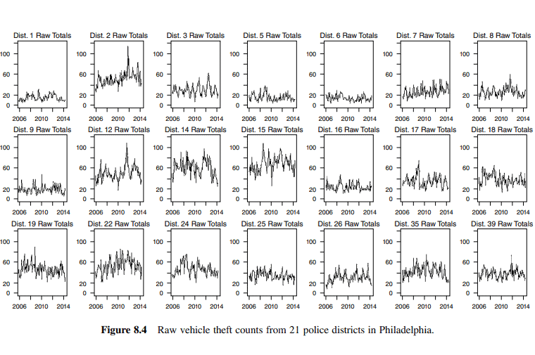
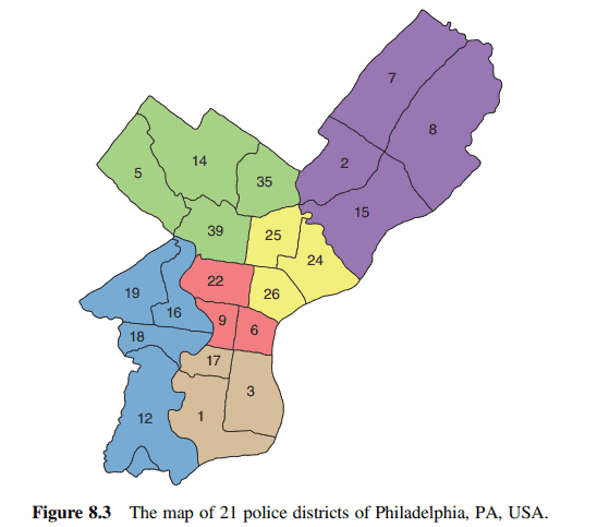
Example 8.5 From January 2006 through December 2014, over 750,000 crimes were reported among the 21 police districts in Philadelphia, Pennsylvania, shown on the map in Figure 8.3. The most common crimes reported were thefts and burglaries. The total crime followed a seasonal pattern with more crimes in the summer than in the winter.
For this analysis, we consider the monthly total of vehicle thefts recorded at the 21 police districts in Philadelphia from January 2006 to December 2014. The data set consists of $m=21$ dimensions corresponding to the 21 police districts and is listed as WW8a in the Data Appendix. The monthly total of vehicle thefts from January 2006 to April 2014 was used for model fitting with a total of $n=100$ observations. The monthly total of the thefts from May 2014 to December 2014 was held out for the forecast comparison. Figure 8.4 displays these raw counts for the in-sample time points.
Visually, each time series shows a constant mean but varies among districts. For the variance, we compare several values for the Box-Cox transformation, and $\lambda=0.5$ is chosen for most locations to stabilize the variance. Thus, the square root of each series was performed. Neither regular nor seasonal differencing was required for any of the 21 series. After being square-root-transformed and mean centered, the resulting 21 series for $t=1,2, \ldots, 100$, is given in Figure 8.5.
Bordering districts are defined as first neighbors, and the weighting matrix for $\mathbf{W}^{(1)}$ is given in Table 8.2. Models involving additional spatial lags were considered but the parameter estimates were not significant different from 0 , and hence the weighting matrices $\mathbf{W}^{(\ell)}$ for $\ell>1$ are not given.
The patterns in Figure 8.6 show that the sample ST-ACFs exponentially decay at both regular time lags, seasonal time lags of multiple of 12 , and that ST-PACFs are significant only at time lags 2,12 , and 24 , and spatial lag at 1 . For a monthly series of seasonal period of 12 , we tentatively choose a $\operatorname{STAR}\left(2_{1,1}\right) \times\left(2_{1,1}\right)_{12}$ as its possible underlying model. The estimation result is given as follows:
Since the estimate of $\phi_{2,1}$ is only 1.46 standard errors away from 0 , we re-fit a STAR $\left(2_{1,0}\right) \times\left(2_{1,1}\right){12}$ model with the following result, $$ \begin{aligned} & \left(\mathbf{I}{21}-\underset{(.031)}{0.128} \mathbf{W}^{(0)} B^{12}-\underset{(.063)}{0.145 \mathbf{W}^{(1)}} B^{12}-\underset{(.033)}{0.058} \mathbf{W}^{(0)} B^{24}-\underset{(.067)}{0.149 \mathbf{W}^{(1)} B^{24}}\right) \ & \left(\mathbf{I}_{21}-\underset{(.029)}{0.336} \mathbf{W}^{(0)} B-\underset{(056)}{0.171 \mathbf{W}^{(1)}} B-\underset{(.034)}{0.121 \mathbf{W}^{(0)}} B^2\right) \mathbf{Z}_t=\mathbf{a}_t . \ & \end{aligned} $$
统计代写|时间序列分析代写Time-Series Analysis代考|The annual U.S. labor force count
Example 8.6 The United States Department of Labor provides dozens of variables through the Bureau of Labor Statistics (BLS), many of which could be fitted with various STARMA models. We select non-seasonally adjusted labor force count for the 48 contiguous states and Washington D.C., for a total of $m=49$ locations. The data are annual from 1976 through 2014 . This constitutes our raw data, which is listed as WW8b in the Data Appendix.
To arrive at the variable $\mathbf{Z}_t$, we already tested and determined that most of the individual time series variables were variance stationary, but appear to have a single unit root. Thus, we took the difference of the counts, and then mean centered the variable for each location. This gives us our zero-mean variable $\mathbf{Z}_t$, with dimension $m=49$ and time points $n=39$. As a side note, one reason for a STARMA-type model to be beneficial for this data is that a VAR(1) model would require $49 \times 49=2401$ parameters, which are more than the number of observations in the data set, and makes the regular VAR fitting impossible. However, the same first order STAR $\left(1_1\right)$ model involves only two parameters.
First, we construct the weighting matrix $\mathbf{W}^{(1)}$ according to the number of bordering states (first neighbors) each state has. Though too large to include for each state in this example, the number of border states ranges from 1 (Maine) to 8 (Missouri and Tennessee). And although not shown, we also construct $\mathbf{W}^{(2)}$ and $\mathbf{W}^{(3)}$ regarding second and third neighbors. Second neighbors are states that do not border each other but have at least one first neighbor in common. These terms are not needed for the chosen STAR $\left(1_1\right)$ model in this example but are included to see if the spatial order is indeed only 1 . Actually, these matrices allow us to construct the sample ST-ACF and ST-PACF, as shown in Tables 8.3 and 8.4.
统计代写|时间序列分析代写Time-Series Analysis代考|Vehicular theft data