分类：时间序列分析代写

统计代写|时间序列分析代写Time-Series Analysis代考|Further generalization and remarks

Posted on 2023年6月15日2023年6月15日 by statistics-lab

如果你也在怎样代写时间序列分析Time-Series Analysis 这个学科遇到相关的难题，请随时右上角联系我们的24/7代写客服。时间序列分析Time-Series Analysis是在数学中，是按时间顺序索引（或列出或绘制）的一系列数据点。最常见的是，一个时间序列是在连续的等距的时间点上的一个序列。因此，它是一个离散时间数据的序列。时间序列的例子有海洋潮汐的高度、太阳黑子的数量和道琼斯工业平均指数的每日收盘值。

时间序列分析Time-Series Analysis分析包括分析时间序列数据的方法，以提取有意义的统计数据和数据的其他特征。时间序列预测是使用一个模型来预测基于先前观察到的值的未来值。虽然经常采用回归分析的方式来测试一个或多个不同时间序列之间的关系，但这种类型的分析通常不被称为 “时间序列分析”，它特别指的是单一序列中不同时间点之间的关系。中断的时间序列分析是用来检测一个时间序列从之前到之后的演变变化，这种变化可能会影响基础变量。

statistics-lab™ 为您的留学生涯保驾护航在代写时间序列分析Time-Series Analysis方面已经树立了自己的口碑, 保证靠谱, 高质且原创的统计Statistics代写服务。我们的专家在代写时间序列分析Time-Series Analysis代写方面经验极为丰富，各种代写时间序列分析Time-Series Analysis相关的作业也就用不着说。

统计代写|时间序列分析代写Time-Series Analysis代考|Further generalization and remarks

More generally, we can include some covariates in all the models introduced in Sections 7.3 and 7.4. For example, when subjects in the model are people, we may want to include related information, such as age, gender, education level, and others, in the model. Thus, we have
$$
Z_{i, j, t}=\mu+c_1 X_{1, j}+\cdots+c_k X_{k, j}+\alpha_i+\beta_t+\gamma_{i, t}+\varepsilon_{i, j, t},
$$
where the $X$ ‘s are covariates with associated coefficients $c$ ‘s.
With proper modifications, the model in (7.37) can be written in matrix form,
$$
\mathbf{Y}=\mathbf{X} \boldsymbol{\beta}+\boldsymbol{\varepsilon}
$$
where the matrix $\mathbf{X}$ will now contain the values of covariates in addition to the values of 0 and 1 for factors, $\boldsymbol{\beta}$ is the vector of the associated parameters, and $\boldsymbol{\varepsilon}$ is a vector of normal random errors with mean vector $\mathbf{0}$ and variance-covariance matrix $\boldsymbol{\Omega}=\mathbf{I}_n \otimes \mathbf{\Sigma}, \mathbf{I}_n$ is the $n \times n$ identity matrix, $n$ is the number of subjects, and $\mathbf{\Sigma}$ is the $(p \times p)$ common variance-covariance structure for all subjects. The GLS estimator of $\boldsymbol{\beta}, \hat{\boldsymbol{\beta}}=\left(\mathbf{X}^{\prime} \mathbf{\Omega}^{-\mathbf{1}} \mathbf{X}\right) \mathbf{X} \boldsymbol{\Omega}^{-\mathbf{1}} \mathbf{Y}$, is the best linear unbiased estimator that follows a multivariate vector normal distribution $N\left(\boldsymbol{\beta},\left(\mathbf{X}^{\prime} \Omega^{-1} \mathbf{X}\right)^{-1}\right)$.

It should be noted that although the examples illustrated in this chapter are equally spaced repeated measurements, the methods introduced can also be applied to cases when repeated measurements are unequally spaced. This is true even when a covariance structure such as an unstructured general covariance, a covariance of independent case, a covariance of common symmetry, or a covariance of heterogeneous common symmetry is used in the analysis. It should be noted, however, that most software such as SAS Proc Mixed may assume equally spaced times when a time series covariance structure like $\operatorname{AR}(1), \operatorname{ARMA}(1,1)$, or the Toeplitz form is specified in the analysis. In such a case, using the software may require some adjustment.

统计代写|时间序列分析代写Time-Series Analysis代考|Another empirical example – the oral condition of neck cancer patients

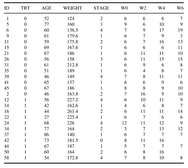
Example 7.3 In this example, we will consider the data set listed in Table 7.9 from the MidMichigan Medical Center for its study of the oral condition of neck cancer patients in 1999 , which is also listed as WW7b in the Data Appendix. The study randomly divided patients into two groups; Group 0 received a placebo and Group 1 received a treatment of aloe juice. The oral conditions of the patients were measured and recorded at the initial stage, and thereafter at the
Table 7.9 Background and oral condition of neck cancer patients under two treatments ( $0=$ placebo, 1 = aloe juice) with total condition at initial stage (Week 0$)$, Week 2 , Week 4 , and Week 6.

end of week 2 , week 4 , and week 6 , respectively. The measurement values varied between 3 and 19 with higher values indicating a better condition. In addition, the age, the initial weight, and the initial cancer stage of patients were also collected. There were a total 25 patients with missing values for patient 42 and 50 . Specifically, we will consider the following model suggested in Eq. (7.37),
$$
Z_{i, j, t}=\mu+c_1 X_{1, j}+c_2 X_{2, j}+c_3 X_{3, j}+\alpha_i+\beta_t+\gamma_{i, t}+\varepsilon_{i, j, t},
$$
where $Z_{i, j, t}$ is the oral condition, $X_{1, j}$ is the patient’s age, $X_{2, j}$ is the patient’s weight at the initial stage, $X_{3, j}$ is the patient’s initial cancer stage, $\alpha_i$ represents the random treatment effect that follows i.i.d. $N\left(0, \sigma_a^2\right), \beta_t$ represents the time effect, $\gamma_{i, t}$ represents time/treatment interaction effect, $\varepsilon_{i, j, t}$ is the error term, and $\alpha_i$ and $\varepsilon_{i, j, t}$ are independent, $i=1,2, n_1=14, n_2=9$, $j=1, \ldots, n_i$, and $t=1,2,3,4$

时间序列分析代考

统计代写|时间序列分析代写Time-Series Analysis代考|Further generalization and remarks

更一般地说，我们可以在7.3节和7.4节介绍的所有模型中包含一些协变量。例如，当模型中的主题是人时，我们可能希望在模型中包含相关信息，如年龄、性别、教育水平等。因此，我们有
$$
Z_{i, j, t}=\mu+c_1 X_{1, j}+\cdots+c_k X_{k, j}+\alpha_i+\beta_t+\gamma_{i, t}+\varepsilon_{i, j, t},
$$
其中$X$ ‘s是协变量与相关系数$c$ ‘s。
通过适当的修改，式(7.37)中的模型可以写成矩阵形式，
$$
\mathbf{Y}=\mathbf{X} \boldsymbol{\beta}+\boldsymbol{\varepsilon}
$$
其中矩阵$\mathbf{X}$现在将包含协变量的值，除了0和1的值为因素，$\boldsymbol{\beta}$是相关参数的向量，$\boldsymbol{\varepsilon}$是正态随机误差的向量，平均向量$\mathbf{0}$和方差协方差矩阵$\boldsymbol{\Omega}=\mathbf{I}_n \otimes \mathbf{\Sigma}, \mathbf{I}_n$是$n \times n$单位矩阵，$n$是受试者的数量，$\mathbf{\Sigma}$是所有被试的共同方差-协方差结构$(p \times p)$。$\boldsymbol{\beta}, \hat{\boldsymbol{\beta}}=\left(\mathbf{X}^{\prime} \mathbf{\Omega}^{-\mathbf{1}} \mathbf{X}\right) \mathbf{X} \boldsymbol{\Omega}^{-\mathbf{1}} \mathbf{Y}$的GLS估计量是遵循多元向量正态分布的最佳线性无偏估计量$N\left(\boldsymbol{\beta},\left(\mathbf{X}^{\prime} \Omega^{-1} \mathbf{X}\right)^{-1}\right)$。

应当指出的是，虽然本章中所示的例子是等间隔重复测量，但所介绍的方法也可以应用于重复测量间隔不等的情况。即使在分析中使用协方差结构，如非结构化的一般协方差、独立情况的协方差、共同对称性的协方差或异质共同对称性的协方差，也是如此。然而，应该注意的是，当时间序列协方差结构(如$\operatorname{AR}(1), \operatorname{ARMA}(1,1)$)或Toeplitz形式在分析中指定时，大多数软件(如SAS Proc Mixed)可能会假设时间间隔等。在这种情况下，使用软件可能需要一些调整。

统计代写|时间序列分析代写Time-Series Analysis代考|Another empirical example – the oral condition of neck cancer patients

例7.3在本例中，我们将考虑表7.9中列出的数据集，该数据集来自MidMichigan Medical Center，用于研究1999年颈癌患者的口腔状况，在数据附录中也被列为WW7b。该研究将患者随机分为两组;0组给予安慰剂，1组给予芦荟汁治疗。在治疗初期和治疗结束后分别测量和记录患者的口腔状况
表7.9接受两种治疗($0=$安慰剂，1 =芦荟汁)的颈部癌症患者的背景和口腔状况，初始阶段(第0周$)$，第2周，第4周和第6周)的总体状况。

第2周，第4周，第6周结束。测量值在3到19之间变化，数值越高表明情况越好。此外，还收集了患者的年龄、初始体重和初始癌症分期。患者42和患者50共有25例患者值缺失。具体来说，我们将考虑Eq.(7.37)中建议的以下模型:
$$
Z_{i, j, t}=\mu+c_1 X_{1, j}+c_2 X_{2, j}+c_3 X_{3, j}+\alpha_i+\beta_t+\gamma_{i, t}+\varepsilon_{i, j, t},
$$
其中$Z_{i, j, t}$为口腔状况，$X_{1, j}$为患者年龄，$X_{2, j}$为患者初期体重，$X_{3, j}$为患者初始癌症分期，$\alpha_i$为i.i.d后随机治疗效果，$N\left(0, \sigma_a^2\right), \beta_t$为时间效应，$\gamma_{i, t}$为时间/治疗交互效应，$\varepsilon_{i, j, t}$为误差项，$\alpha_i$和$\varepsilon_{i, j, t}$为独立项。$i=1,2, n_1=14, n_2=9$, $j=1, \ldots, n_i$，和 $t=1,2,3,4$

统计代写|时间序列分析代写Time-Series Analysis代考请认准statistics-lab™

统计代写请认准statistics-lab™. statistics-lab™为您的留学生涯保驾护航。

金融工程代写

金融工程是使用数学技术来解决金融问题。金融工程使用计算机科学、统计学、经济学和应用数学领域的工具和知识来解决当前的金融问题，以及设计新的和创新的金融产品。

非参数统计代写

非参数统计指的是一种统计方法，其中不假设数据来自于由少数参数决定的规定模型；这种模型的例子包括正态分布模型和线性回归模型。

广义线性模型代考

广义线性模型（GLM）归属统计学领域，是一种应用灵活的线性回归模型。该模型允许因变量的偏差分布有除了正态分布之外的其它分布。

术语广义线性模型（GLM）通常是指给定连续和/或分类预测因素的连续响应变量的常规线性回归模型。它包括多元线性回归，以及方差分析和方差分析（仅含固定效应）。

有限元方法代写

有限元方法（FEM）是一种流行的方法，用于数值解决工程和数学建模中出现的微分方程。典型的问题领域包括结构分析、传热、流体流动、质量运输和电磁势等传统领域。

有限元是一种通用的数值方法，用于解决两个或三个空间变量的偏微分方程（即一些边界值问题）。为了解决一个问题，有限元将一个大系统细分为更小、更简单的部分，称为有限元。这是通过在空间维度上的特定空间离散化来实现的，它是通过构建对象的网格来实现的：用于求解的数值域，它有有限数量的点。边界值问题的有限元方法表述最终导致一个代数方程组。该方法在域上对未知函数进行逼近。[1] 然后将模拟这些有限元的简单方程组合成一个更大的方程系统，以模拟整个问题。然后，有限元通过变化微积分使相关的误差函数最小化来逼近一个解决方案。

tatistics-lab作为专业的留学生服务机构，多年来已为美国、英国、加拿大、澳洲等留学热门地的学生提供专业的学术服务，包括但不限于Essay代写，Assignment代写，Dissertation代写，Report代写，小组作业代写，Proposal代写，Paper代写，Presentation代写，计算机作业代写，论文修改和润色，网课代做，exam代考等等。写作范围涵盖高中，本科，研究生等海外留学全阶段，辐射金融，经济学，会计学，审计学，管理学等全球99%专业科目。写作团队既有专业英语母语作者，也有海外名校硕博留学生，每位写作老师都拥有过硬的语言能力，专业的学科背景和学术写作经验。我们承诺100%原创，100%专业，100%准时，100%满意。

随机分析代写

随机微积分是数学的一个分支，对随机过程进行操作。它允许为随机过程的积分定义一个关于随机过程的一致的积分理论。这个领域是由日本数学家伊藤清在第二次世界大战期间创建并开始的。

时间序列分析代写

随机过程，是依赖于参数的一组随机变量的全体，参数通常是时间。随机变量是随机现象的数量表现，其时间序列是一组按照时间发生先后顺序进行排列的数据点序列。通常一组时间序列的时间间隔为一恒定值（如1秒，5分钟，12小时，7天，1年），因此时间序列可以作为离散时间数据进行分析处理。研究时间序列数据的意义在于现实中，往往需要研究某个事物其随时间发展变化的规律。这就需要通过研究该事物过去发展的历史记录，以得到其自身发展的规律。

回归分析代写

多元回归分析渐进（Multiple Regression Analysis Asymptotics）属于计量经济学领域，主要是一种数学上的统计分析方法，可以分析复杂情况下各影响因素的数学关系，在自然科学、社会和经济学等多个领域内应用广泛。

MATLAB代写

MATLAB 是一种用于技术计算的高性能语言。它将计算、可视化和编程集成在一个易于使用的环境中，其中问题和解决方案以熟悉的数学符号表示。典型用途包括：数学和计算算法开发建模、仿真和原型制作数据分析、探索和可视化科学和工程图形应用程序开发，包括图形用户界面构建MATLAB 是一个交互式系统，其基本数据元素是一个不需要维度的数组。这使您可以解决许多技术计算问题，尤其是那些具有矩阵和向量公式的问题，而只需用 C 或 Fortran 等标量非交互式语言编写程序所需的时间的一小部分。MATLAB 名称代表矩阵实验室。MATLAB 最初的编写目的是提供对由 LINPACK 和 EISPACK 项目开发的矩阵软件的轻松访问，这两个项目共同代表了矩阵计算软件的最新技术。MATLAB 经过多年的发展，得到了许多用户的投入。在大学环境中，它是数学、工程和科学入门和高级课程的标准教学工具。在工业领域，MATLAB 是高效研究、开发和分析的首选工具。MATLAB 具有一系列称为工具箱的特定于应用程序的解决方案。对于大多数 MATLAB 用户来说非常重要，工具箱允许您学习和应用专业技术。工具箱是 MATLAB 函数（M 文件）的综合集合，可扩展 MATLAB 环境以解决特定类别的问题。可用工具箱的领域包括信号处理、控制系统、神经网络、模糊逻辑、小波、仿真等。

R语言代写	问卷设计与分析代写
PYTHON代写	回归分析与线性模型代写
MATLAB代写	方差分析与试验设计代写
STATA代写	机器学习/统计学习代写
SPSS代写	计量经济学代写
EVIEWS代写	时间序列分析代写
EXCEL代写	深度学习代写
SQL代写	各种数据建模与可视化代写

统计代写|时间序列分析代写Time-Series Analysis代考|Asymptotic distribution and statistical inference

Posted on 2023年6月15日2023年6月15日 by statistics-lab

统计代写|时间序列分析代写Time-Series Analysis代考|Asymptotic distribution and statistical inference

Properties and statistical inferences are easy to derive for distributions that are elliptically symmetric. Unfortunately, the closed-form of the distribution of $\mathbf{r}t$ is unknown, and it is certainly not elliptically symmetric under the GO-GARCH model. We study the distribution of the estimator $\hat{\mathbf{V}}_w$ based on the influence function (IF), first introduced by Hampel et al. (1986). For simplicity, we assume that all functionals discussed here are Frechet differentiable. For a fixed point $\mathbf{x} \in R^m$, let $\delta{\mathbf{x}}$ be the point-mass probability measure that assigns mass 1 to $\mathbf{x}$. The influence function of the functional $K(\cdot)$ at a fixed point $\mathbf{x}$ and the given distribution $F$ is defined as:
$$
I F(\mathbf{x} ; F, K)=\lim {c \rightarrow 0^{+}} \frac{K\left[(1-c) F+c \delta{\mathbf{x}}\right]-K(F)}{c}
$$
where ” $\rightarrow 0^{+,}$stands for limit from the right of zero, $\delta_{\mathbf{x}}$ is the point mass at $\mathbf{x}$. Clearly, the influence function measures the relative effect on the functional $K(\cdot)$ of an infinitesimal point-mass contamination of the distribution $F$.

We derive the $I F$ of $\mathbf{v}{w, i}$, measuring changes of $\mathbf{v}{w, i}$ under infinitesimal change of $F_{\mathrm{s}}$. Let $\mathbf{r}^=\left(r_1^, \ldots, r_m^\right)^{\prime}=\operatorname{diag}\left(k_{w, 1}^{-1 / 2}, \ldots, k_{w, m}^{-1 / 2}\right) \mathbf{V}w \mathbf{s}$, where $k{w, 1}, \ldots, k_{w, m}$ are the eigenvalues of $\mathbf{H}w$, ordered corresponding to the associated columns of $\mathbf{V}_w$, and $\mathbf{s}$ is a $(m \times 1)$ random vector. Define $\mathbf{W}$ to be a $m \times m$ matrix with diagonal elements $W{i, i}=2+E\left[w\left(\left|\mathbf{r}^\right|^2\left(r_i^\right)^4\right) /\left|\mathbf{r}^\right|\right]$ and off-diagonal elements $W_{i, j}=E\left[w\left(\left|\mathbf{r}^\right|^2\left(r_i^\right)^2\left(r_j^\right)^2\right) /\left|\mathbf{r}^\right|\right], i, j=1, \ldots, m, i \neq j$, where $|\cdot|$ denotes the Euclidean norm. Assuming that $E\left(r_i^4\right)<\infty$ and $\mathbf{W}$ is nonsingular, we have the following theorem:

Theorem 6.3 The influence function of $\mathbf{v}{w, i}$ at $F{\mathrm{s}}$ and a fixed point $\mathbf{s}0 \in R^m$ is given by: $$ I F\left(\mathbf{s}_0 ; F_s, \mathbf{v}{w, i}\right)=\sum_{j \neq 1, j \neq i}^m \frac{\sqrt{k_{w, i} k_{w, j}} w\left(\left|\mathbf{r}0^\right|^2\right) r{i, 0}^ r_{j, 0}^}{\left(k_{w, i}-k_{w, j}\right)\left[1+E\left{\frac{w\left(\left|\mathbf{r}^\right|^2\right)}{\left|\mathbf{r}^\right|}\left(r_i^\right)^2\left(r_j^\right)^2\right}\right]} \mathbf{v}{w, j}, $$ where $\mathbf{r}_0^=\left(r{1,0}^, \ldots, r_{m, 0}^\right)^{\prime}=\operatorname{diag}\left(k_{w, 1}^{-1 / 2}, \ldots, k_{w, m}^{-1 / 2}\right) \mathbf{V}_w \mathbf{s}_0$. For the proof, please see Zheng and Wei (2012).

We derive the asymptotic distribution of our weighted scatter estimators based on the influence function. Under regularity conditions (Hampel et al. (1986), and Huber (1981), we have:
$$
T^{1 / 2}\left(\hat{\mathbf{v}}{w, i}-\mathbf{v}_i\right) \stackrel{d}{\rightarrow} N\left{\mathbf{0}, A S V\left(\mathbf{v}{w, i}, F_{\mathrm{s}}\right)\right}
$$
where
$$
\begin{aligned}
\operatorname{ASV}\left(\mathbf{v}{w, i}, F{\mathrm{s}}\right) & =E\left{\left[I F\left(\mathbf{s}0 ; F{\mathrm{s}}, \mathbf{v}{w, i}\right)\right]\left[I F\left(\mathbf{s}_0 ; F{\mathrm{s}}, \mathbf{v}{w, i}\right)\right]^{\prime}\right} \ & =\sum{j \neq 1, j \neq i}^m \frac{k_{w, i} k_{w, j} E\left{\left[w\left(\left|\mathbf{r}0^\right|^2\right)\right]^2\left(r{i, 0}^\right)^2\left(r_{j, 0}^\right)^2\right}}{\left(k_{w, i}-k_{w, j}\right)^2\left[1+E\left{\frac{w^{\prime}\left(\left|\mathbf{r}^\right|^2\right)}{\left|\mathbf{r}^\right|}\left(r_i^\right)^2\left(r_j^*\right)^2\right}\right]^2} \mathbf{v}{w, j} \mathbf{v}{w, j}^{\prime} .
\end{aligned}
$$

统计代写|时间序列分析代写Time-Series Analysis代考|Combining information from different weighting functions

While the determination of the weighting function is arbitrary, we may obtain more efficient estimation results by combining information from different weighting functions. Denote $\hat{\mathbf{V}}{w, 1}, \ldots, \hat{\mathbf{V}}{w, k}$ to be $k$ estimators of $\mathbf{V}$ matrix based on $k$ different weighting functions. We can pool them together using the Cayley transformation (see Liebeck and Osborne [1991]):
$$
\hat{\mathbf{V}}w=\left{\mathbf{I}_m-\sum{i=1}^k\left[p_i\left(\mathbf{I}m-\hat{\mathbf{V}}{w, i}\right)\right]\left(\mathbf{I}m-\hat{\mathbf{V}}{w, i}\right)^{-1}\right}\left{\mathbf{I}m+\sum{i=1}^k\left[p_i\left(\mathbf{I}m-\hat{\mathbf{V}}{w, i}\right)\right]\left(\mathbf{I}m-\hat{\mathbf{V}}{w, i}\right)^{-1}\right}^{-1},
$$
where $p_i$ ‘s are some weighting functions satisfying $\sum_{i=1}^k p_i=1$. The weights $p_i^{\prime} s$ are chosen to be dependent on the closeness of eigenvalues of the $k$ weighted scatter estimators, $\hat{\mathbf{H}}{w, 1}, \ldots$, and $\hat{\mathbf{H}}{w, k}$. For example, let the eigenvalues of $\hat{\mathbf{H}}{w, i}$ to be $\hat{\lambda}{1, i}, \ldots, \hat{\lambda}{m, i}, i=1, \ldots, k$, we choose: $$ p_i=\frac{\min {1 \leq \ell<j \leq m}\left(\hat{\lambda}{\ell, i}-\hat{\lambda}{j, i}\right)^2}{\sum_{i=1}^k \min {1 \leq \ell{\ell, i}-\hat{\lambda}{j, i}\right)^2} $$ Thus, if any two eigenvalues of a weighted multivariate scatter estimator are close, the weight of the associated estimator $\hat{\mathbf{V}}{w, i}$ receives a small weight. This provides protection against possible identification problems. Since the estimation of $\mathbf{V}$ is up to multiplying a permutation matrix with entries of $0,+1$ or -1 , care must be taken. Orthogonal matrices $\hat{\mathbf{V}}{w, \ell}, \ell=2$, $\ldots, k$, are matched as closely as possible to $\hat{\mathbf{V}}{w, 1}$. The $i$ th row of the matched matrix $\hat{\mathbf{V}}{w, \ell}$, denoted $\hat{\mathbf{v}}{w, \ell, i}^{\prime}$, satisfies:
$$
\left|\hat{\mathbf{v}}{w, \ell, i}^{\prime} \hat{\mathbf{v}}{w, \ell, i}\right|=\max {i \leq j \leq m}\left|\hat{\mathbf{v}}{w, \ell, j}^{\prime} \hat{\mathbf{v}}_{w, \ell, i}\right|
$$

时间序列分析代考

统计代写|时间序列分析代写Time-Series Analysis代考|Asymptotic distribution and statistical inference

对于椭圆对称的分布，性质和统计推论很容易推导出来。遗憾的是，$\mathbf{r}t$分布的封闭形式是未知的，在GO-GARCH模型下，它肯定不是椭圆对称的。我们研究了基于影响函数(IF)的估计量$\hat{\mathbf{V}}w$的分布，该函数首先由Hampel et al.(1986)引入。为简单起见，我们假设这里讨论的所有泛函都是Frechet可微的。对于固定点$\mathbf{x} \in R^m$，设$\delta{\mathbf{x}}$为将质量1赋给$\mathbf{x}$的点-质量概率测度。函数$K(\cdot)$在不动点$\mathbf{x}$与给定分布$F$的影响函数定义为: $$ I F(\mathbf{x} ; F, K)=\lim {c \rightarrow 0^{+}} \frac{K\left[(1-c) F+c \delta{\mathbf{x}}\right]-K(F)}{c} $$ 其中“$\rightarrow 0^{+,}$”表示从零右边开始的极限，$\delta{\mathbf{x}}$是$\mathbf{x}$处的质点。显然，影响函数测量了分布$F$的无限小点质量污染对函数$K(\cdot)$的相对影响。

我们推导出$\mathbf{v}{w, i}$的$I F$，在$F_{\mathrm{s}}$的无穷小变化下测量$\mathbf{v}{w, i}$的变化。设$\mathbf{r}^=\left(r_1^, \ldots, r_m^\right)^{\prime}=\operatorname{diag}\left(k_{w, 1}^{-1 / 2}, \ldots, k_{w, m}^{-1 / 2}\right) \mathbf{V}w \mathbf{s}$，其中$k{w, 1}, \ldots, k_{w, m}$为$\mathbf{H}w$的特征值，顺序对应于$\mathbf{V}w$的关联列，$\mathbf{s}$为$(m \times 1)$随机向量。定义$\mathbf{W}$为具有对角元素$W{i, i}=2+E\left[w\left(\left|\mathbf{r}^\right|^2\left(r_i^\right)^4\right) /\left|\mathbf{r}^\right|\right]$和非对角元素$W{i, j}=E\left[w\left(\left|\mathbf{r}^\right|^2\left(r_i^\right)^2\left(r_j^\right)^2\right) /\left|\mathbf{r}^\right|\right], i, j=1, \ldots, m, i \neq j$的$m \times m$矩阵，其中$|\cdot|$表示欧几里得范数。假设$E\left(r_i^4\right)<\infty$和$\mathbf{W}$为非奇异，则有以下定理:

定理6.3 $\mathbf{v}{w, i}$在$F{\mathrm{s}}$与不动点$\mathbf{s}0 \in R^m$处的影响函数为:$$ I F\left(\mathbf{s}0 ; F_s, \mathbf{v}{w, i}\right)=\sum{j \neq 1, j \neq i}^m \frac{\sqrt{k_{w, i} k_{w, j}} w\left(\left|\mathbf{r}0^\right|^2\right) r{i, 0}^ r_{j, 0}^}{\left(k_{w, i}-k_{w, j}\right)\left[1+E\left{\frac{w\left(\left|\mathbf{r}^\right|^2\right)}{\left|\mathbf{r}^\right|}\left(r_i^\right)^2\left(r_j^\right)^2\right}\right]} \mathbf{v}{w, j}, $$其中$\mathbf{r}0^=\left(r{1,0}^, \ldots, r{m, 0}^\right)^{\prime}=\operatorname{diag}\left(k_{w, 1}^{-1 / 2}, \ldots, k_{w, m}^{-1 / 2}\right) \mathbf{V}_w \mathbf{s}_0$。关于证明，请参见Zheng and Wei(2012)。

基于影响函数导出了加权散点估计量的渐近分布。在正则性条件下(Hampel et al.(1986)和Huber(1981))，我们有:
$$
T^{1 / 2}\left(\hat{\mathbf{v}}{w, i}-\mathbf{v}i\right) \stackrel{d}{\rightarrow} N\left{\mathbf{0}, A S V\left(\mathbf{v}{w, i}, F{\mathrm{s}}\right)\right}
$$
在哪里
$$
\begin{aligned}
\operatorname{ASV}\left(\mathbf{v}{w, i}, F{\mathrm{s}}\right) & =E\left{\left[I F\left(\mathbf{s}0 ; F{\mathrm{s}}, \mathbf{v}{w, i}\right)\right]\left[I F\left(\mathbf{s}0 ; F{\mathrm{s}}, \mathbf{v}{w, i}\right)\right]^{\prime}\right} \ & =\sum{j \neq 1, j \neq i}^m \frac{k{w, i} k_{w, j} E\left{\left[w\left(\left|\mathbf{r}0^\right|^2\right)\right]^2\left(r{i, 0}^\right)^2\left(r_{j, 0}^\right)^2\right}}{\left(k_{w, i}-k_{w, j}\right)^2\left[1+E\left{\frac{w^{\prime}\left(\left|\mathbf{r}^\right|^2\right)}{\left|\mathbf{r}^\right|}\left(r_i^\right)^2\left(r_j^*\right)^2\right}\right]^2} \mathbf{v}{w, j} \mathbf{v}{w, j}^{\prime} .
\end{aligned}
$$

统计代写|时间序列分析代写Time-Series Analysis代考|Combining information from different weighting functions

虽然权重函数的确定是任意的，但将不同权重函数的信息组合起来可以得到更有效的估计结果。表示$\hat{\mathbf{V}}{w, 1}, \ldots, \hat{\mathbf{V}}{w, k}$为基于$k$不同权重函数的$\mathbf{V}$矩阵的$k$估计量。我们可以使用Cayley变换(参见Liebeck和Osborne[1991])将它们汇集在一起:
$$
\hat{\mathbf{V}}w=\left{\mathbf{I}m-\sum{i=1}^k\left[p_i\left(\mathbf{I}m-\hat{\mathbf{V}}{w, i}\right)\right]\left(\mathbf{I}m-\hat{\mathbf{V}}{w, i}\right)^{-1}\right}\left{\mathbf{I}m+\sum{i=1}^k\left[p_i\left(\mathbf{I}m-\hat{\mathbf{V}}{w, i}\right)\right]\left(\mathbf{I}m-\hat{\mathbf{V}}{w, i}\right)^{-1}\right}^{-1}, $$ 其中$p_i$为满足$\sum{i=1}^k p_i=1$的权重函数。权重$p_i^{\prime} s$的选择取决于$k$加权散点估计器、$\hat{\mathbf{H}}{w, 1}, \ldots$和$\hat{\mathbf{H}}{w, k}$的特征值的接近程度。例如，设$\hat{\mathbf{H}}{w, i}$的特征值为$\hat{\lambda}{1, i}, \ldots, \hat{\lambda}{m, i}, i=1, \ldots, k$，我们选择:$$ p_i=\frac{\min {1 \leq \ell<j \leq m}\left(\hat{\lambda}{\ell, i}-\hat{\lambda}{j, i}\right)^2}{\sum_{i=1}^k \min {1 \leq \ell{\ell, i}-\hat{\lambda}{j, i}\right)^2} $$因此，如果一个加权多变量散点估计量的任意两个特征值接近，则关联估计量$\hat{\mathbf{V}}{w, i}$的权值收到一个小的权值。这为可能出现的识别问题提供了保护。由于$\mathbf{V}$的估计取决于将一个排列矩阵与条目$0,+1$或-1相乘，因此必须小心。正交矩阵$\hat{\mathbf{V}}{w, \ell}, \ell=2$, $\ldots, k$，尽可能与$\hat{\mathbf{V}}{w, 1}$匹配。匹配矩阵$\hat{\mathbf{V}}{w, \ell}$(记为$\hat{\mathbf{v}}{w, \ell, i}^{\prime}$)的第$i$行满足:
$$
\left|\hat{\mathbf{v}}{w, \ell, i}^{\prime} \hat{\mathbf{v}}{w, \ell, i}\right|=\max {i \leq j \leq m}\left|\hat{\mathbf{v}}{w, \ell, j}^{\prime} \hat{\mathbf{v}}_{w, \ell, i}\right|
$$

统计代写请认准statistics-lab™. statistics-lab™为您的留学生涯保驾护航。

金融工程代写

非参数统计代写

非参数统计指的是一种统计方法，其中不假设数据来自于由少数参数决定的规定模型；这种模型的例子包括正态分布模型和线性回归模型。

广义线性模型代考

广义线性模型（GLM）归属统计学领域，是一种应用灵活的线性回归模型。该模型允许因变量的偏差分布有除了正态分布之外的其它分布。

有限元方法代写

随机分析代写

时间序列分析代写

回归分析代写

MATLAB代写

R语言代写	问卷设计与分析代写
PYTHON代写	回归分析与线性模型代写
MATLAB代写	方差分析与试验设计代写
STATA代写	机器学习/统计学习代写
SPSS代写	计量经济学代写
EVIEWS代写	时间序列分析代写
EXCEL代写	深度学习代写
SQL代写	各种数据建模与可视化代写

统计代写|时间序列分析代写Time-Series Analysis代考|Constant Conditional Correlation (CCC) models

Posted on 2023年5月29日2023年5月29日 by statistics-lab

统计代写|时间序列分析代写Time-Series Analysis代考|Factor analysis

One other way to reduce the number of parameters in the VEC model was suggested by Bollerslev (1990) who proposed a representation where the conditional correlation matrix is assumed to be constant. Under such an assumption, the conditional covariances are proportional to the product of the corresponding conditional standard deviations. The model becomes
$$
\boldsymbol{\Sigma}t=\mathbf{D}_t \mathbf{R D}_t $$ where $$ \begin{gathered} D_t=\operatorname{diag}\left(\sigma{1,1, t}^{1 / 2}, \ldots, \sigma_{m, m, t}^{1 / 2}\right), \
R=\left[\begin{array}{ccccc}
1 & \rho_{1,2} & \cdots & \cdots & \rho_{1, m} \
\rho_{1,2} & 1 & \cdots & \cdots & \rho_{2, m} \
\vdots & \vdots & \ddots & \vdots & \vdots \
\vdots & \vdots & \vdots & \ddots & \vdots \
\rho_{1, m} & \rho_{2, m} & \cdots & \cdots & 1
\end{array}\right],
\end{gathered}
$$
and $\rho_{i, j}$ is the constant conditional correlation between $\varepsilon_{i, t}$ and $\varepsilon_{j, t}$. The representation is known as the constant conditional correlation (CCC) model. Thus,
$$
\sigma_{i, j, t}=\rho_{i, j} \sqrt{\sigma_{i, i, t} \sigma_{j, j, t}}
$$
and $\sigma_{i, i, t}$ can be modeled independently as univariate GARCH models like the simple GARCH $(1,1)$ model,
$$
\sigma_{i, i, t}=c_i+\alpha_i \sigma_{i, i, t-1}+\beta_i \varepsilon_{i, t-1}^2, i=1, \ldots, m
$$

统计代写|时间序列分析代写Time-Series Analysis代考|BEKK models

Other than the large number of parameters in the model, the other problem with the VEC model is that the conditional covariance matrix as formulated in Eq. (6.6) may not be positive definite. To overcome the difficulty, Engle and Kroner (1995) used a quadratic form to propose the following model, which, without including exogenous variables, is given by
$$
\boldsymbol{\Sigma}t=\mathbf{C}^{\prime} \mathbf{C}+\sum{j=1}^p \boldsymbol{\Phi}j^{\prime} \boldsymbol{\Sigma}{t-1} \boldsymbol{\Phi}j+\sum{j=1}^q \boldsymbol{\Theta}j^{\prime} \varepsilon{t-1} \boldsymbol{\varepsilon}{t-1}^{\prime} \boldsymbol{\Theta}_j, $$ where $\mathbf{C}$ is a $m \times m$ triangular matrix, which is to ensure $\boldsymbol{\Sigma}_t$ to be definitely positive. Engle and Kroner call it BEKK model because it is related to their earlier joint work of Baba et al. (1990). For convenience, we will call the model in Eq. (6.15) as $\operatorname{BEKK}(p, q)$ model. The BEKK(1,1) model is $$ \boldsymbol{\Sigma}_t=\mathbf{C}^{\prime} \mathbf{C}+\boldsymbol{\Phi}_1^{\prime} \boldsymbol{\Sigma}{t-1} \boldsymbol{\Phi}1+\boldsymbol{\Theta}_1^{\prime} \boldsymbol{\varepsilon}{t-1} \boldsymbol{\varepsilon}_{t-1}^{\prime} \boldsymbol{\Theta}_1
$$

The model will be stationary if and only if the eigenvalues of $\boldsymbol{\Phi}1^{\prime} \otimes \boldsymbol{\Phi}_1+\boldsymbol{\Theta}_1^{\prime} \otimes \boldsymbol{\Theta}_1$ are in the unit circle, where $\otimes$ is the Kronecker product of two matrices. For a two-dimensional BEKK $(1,1)$ model, its explicit form is given by $$ \begin{aligned} \boldsymbol{\Sigma}_t= & {\left[\begin{array}{ll} \sigma{1,1, t} & \sigma_{1,2, t} \
\sigma_{1,2, t} & \sigma_{2,2, t}
\end{array}\right]=\left[\begin{array}{ll}
c_{1,1} & c_{1,2} \
c_{2,1} & c_{2,2}
\end{array}\right]+\left[\begin{array}{ll}
\phi_{1,1} & \phi_{1,2} \
\phi_{2,1} & \phi_{2,2}
\end{array}\right]^{\prime}\left[\begin{array}{ll}
\sigma_{1,1, t-1} & \sigma_{1,2, t-1} \
\sigma_{1,2, t-1} & \sigma_{2,2, t-1}
\end{array}\right]\left[\begin{array}{ll}
\phi_{1,1} & \phi_{1,2} \
\phi_{2,1} & \phi_{2,2}
\end{array}\right] } \
& +\left[\begin{array}{ll}
\theta_{1,1} & \theta_{1,2} \
\theta_{2,1} & \theta_{2,2}
\end{array}\right]^{\prime}\left[\begin{array}{cc}
\varepsilon_{1, t-1}^2 & \varepsilon_{1, t-1} \varepsilon_{2, t-1} \
\varepsilon_{2, t-1} \varepsilon_{1, t-1} & \varepsilon_{2, t-1}^2
\end{array}\right]\left[\begin{array}{ll}
\theta_{1,1} & \theta_{1,2} \
\theta_{2,1} & \theta_{2,2}
\end{array}\right],
\end{aligned}
$$
and hence,
$$
\begin{aligned}
\sigma_{1,1, t}= & c_{1,1}+\phi_{1,1}^2 \sigma_{1,1, t-1}+2 \phi_{1,1} \phi_{2,1} \sigma_{1,2, t-1}+\phi_{2,1}^2 \sigma_{2,2, t-1} \
& +\theta_{1,1}^2 \varepsilon_{1, t-1}^2+2 \theta_{1,1} \theta_{2,1} \varepsilon_{1, t-1} \varepsilon_{2, t-1}+\theta_{2,1}^2 \varepsilon_{2, t-1}^2 \
\sigma_{1,2, t}= & c_{1,2}+\phi_{1,1} \phi_{1,2} \sigma_{1,1, t-1}+\left(\phi_{1,1} \phi_{2,2}+\phi_{1,2} \phi_{2,1}\right) \sigma_{1,2, t-1}+\phi_{2,1} \phi_{2,2} \sigma_{2,2, t-1} \
& +\theta_{1,1} \theta_{1,2} \varepsilon_{1, t-1}^2+\left(\theta_{1,1} \theta_{2,2}+\theta_{1,2} \theta_{2,1}\right) \varepsilon_{1, t-1} \varepsilon_{2, t-1}+\theta_{2,1} \theta_{2,2} \varepsilon_{2, t-1}^2, \
\sigma_{2,2, t}= & c_{2,2}+\phi_{1,2}^2 \sigma_{1,1, t-1}+2 \phi_{1,1} \phi_{2,2} \sigma_{1,2, t-1}+\phi_{2,2}^2 \sigma_{2,2, t-1} \
& +\theta_{1,2}^2 \varepsilon_{1, t-1}^2+2 \theta_{1,2} \theta_{2,2} \varepsilon_{1, t-1} \varepsilon_{2, t-1}+\theta_{2,1}^2 \varepsilon_{2, t-1}^2,
\end{aligned}
$$

时间序列分析代考

统计代写|时间序列分析代写Time-Series Analysis代考|Factor analysis

Bollerslev(1990)提出了另一种减少VEC模型中参数数量的方法，他提出了一种假设条件相关矩阵为常数的表示。在这种假设下，条件协方差与相应条件标准差的乘积成正比。模型变成了
$$
\boldsymbol{\Sigma}t=\mathbf{D}t \mathbf{R D}_t $$ where $$ \begin{gathered} D_t=\operatorname{diag}\left(\sigma{1,1, t}^{1 / 2}, \ldots, \sigma{m, m, t}^{1 / 2}\right), \
R=\left[\begin{array}{ccccc}
1 & \rho_{1,2} & \cdots & \cdots & \rho_{1, m} \
\rho_{1,2} & 1 & \cdots & \cdots & \rho_{2, m} \
\vdots & \vdots & \ddots & \vdots & \vdots \
\vdots & \vdots & \vdots & \ddots & \vdots \
\rho_{1, m} & \rho_{2, m} & \cdots & \cdots & 1
\end{array}\right],
\end{gathered}
$$
$\rho_{i, j}$是$\varepsilon_{i, t}$和$\varepsilon_{j, t}$之间的常数条件相关。这种表示称为恒定条件相关(CCC)模型。因此，
$$
\sigma_{i, j, t}=\rho_{i, j} \sqrt{\sigma_{i, i, t} \sigma_{j, j, t}}
$$
和$\sigma_{i, i, t}$可以独立建模为单变量GARCH模型，就像简单的GARCH $(1,1)$模型一样，
$$
\sigma_{i, i, t}=c_i+\alpha_i \sigma_{i, i, t-1}+\beta_i \varepsilon_{i, t-1}^2, i=1, \ldots, m
$$

统计代写|时间序列分析代写Time-Series Analysis代考|BEKK models

除了模型中有大量的参数外，VEC模型的另一个问题是公式(6.6)中的条件协方差矩阵可能不是正定的。为了克服这一困难，Engle和Kroner(1995)使用二次型提出了以下模型，该模型不包括外生变量，由
$$
\boldsymbol{\Sigma}t=\mathbf{C}^{\prime} \mathbf{C}+\sum{j=1}^p \boldsymbol{\Phi}j^{\prime} \boldsymbol{\Sigma}{t-1} \boldsymbol{\Phi}j+\sum{j=1}^q \boldsymbol{\Theta}j^{\prime} \varepsilon{t-1} \boldsymbol{\varepsilon}{t-1}^{\prime} \boldsymbol{\Theta}j, $$其中$\mathbf{C}$是一个$m \times m$三角矩阵，这是为了保证$\boldsymbol{\Sigma}_t$是肯定的正数。Engle和Kroner称其为BEKK模型，因为它与他们早期Baba等人(1990)的联合研究有关。为方便起见，我们将式(6.15)中的模型称为$\operatorname{BEKK}(p, q)$模型。BEKK(1,1)模型为 $$ \boldsymbol{\Sigma}_t=\mathbf{C}^{\prime} \mathbf{C}+\boldsymbol{\Phi}_1^{\prime} \boldsymbol{\Sigma}{t-1} \boldsymbol{\Phi}1+\boldsymbol{\Theta}_1^{\prime} \boldsymbol{\varepsilon}{t-1} \boldsymbol{\varepsilon}{t-1}^{\prime} \boldsymbol{\Theta}_1
$$

当且仅当$\boldsymbol{\Phi}1^{\prime} \otimes \boldsymbol{\Phi}1+\boldsymbol{\Theta}_1^{\prime} \otimes \boldsymbol{\Theta}_1$的特征值在单位圆内时，模型是平稳的，其中$\otimes$是两个矩阵的Kronecker积。对于二维BEKK $(1,1)$模型，其显式形式为$$ \begin{aligned} \boldsymbol{\Sigma}_t= & {\left[\begin{array}{ll} \sigma{1,1, t} & \sigma{1,2, t} \
\sigma_{1,2, t} & \sigma_{2,2, t}
\end{array}\right]=\left[\begin{array}{ll}
c_{1,1} & c_{1,2} \
c_{2,1} & c_{2,2}
\end{array}\right]+\left[\begin{array}{ll}
\phi_{1,1} & \phi_{1,2} \
\phi_{2,1} & \phi_{2,2}
\end{array}\right]^{\prime}\left[\begin{array}{ll}
\sigma_{1,1, t-1} & \sigma_{1,2, t-1} \
\sigma_{1,2, t-1} & \sigma_{2,2, t-1}
\end{array}\right]\left[\begin{array}{ll}
\phi_{1,1} & \phi_{1,2} \
\phi_{2,1} & \phi_{2,2}
\end{array}\right] } \
& +\left[\begin{array}{ll}
\theta_{1,1} & \theta_{1,2} \
\theta_{2,1} & \theta_{2,2}
\end{array}\right]^{\prime}\left[\begin{array}{cc}
\varepsilon_{1, t-1}^2 & \varepsilon_{1, t-1} \varepsilon_{2, t-1} \
\varepsilon_{2, t-1} \varepsilon_{1, t-1} & \varepsilon_{2, t-1}^2
\end{array}\right]\left[\begin{array}{ll}
\theta_{1,1} & \theta_{1,2} \
\theta_{2,1} & \theta_{2,2}
\end{array}\right],
\end{aligned}
$$
因此，
$$
\begin{aligned}
\sigma_{1,1, t}= & c_{1,1}+\phi_{1,1}^2 \sigma_{1,1, t-1}+2 \phi_{1,1} \phi_{2,1} \sigma_{1,2, t-1}+\phi_{2,1}^2 \sigma_{2,2, t-1} \
& +\theta_{1,1}^2 \varepsilon_{1, t-1}^2+2 \theta_{1,1} \theta_{2,1} \varepsilon_{1, t-1} \varepsilon_{2, t-1}+\theta_{2,1}^2 \varepsilon_{2, t-1}^2 \
\sigma_{1,2, t}= & c_{1,2}+\phi_{1,1} \phi_{1,2} \sigma_{1,1, t-1}+\left(\phi_{1,1} \phi_{2,2}+\phi_{1,2} \phi_{2,1}\right) \sigma_{1,2, t-1}+\phi_{2,1} \phi_{2,2} \sigma_{2,2, t-1} \
& +\theta_{1,1} \theta_{1,2} \varepsilon_{1, t-1}^2+\left(\theta_{1,1} \theta_{2,2}+\theta_{1,2} \theta_{2,1}\right) \varepsilon_{1, t-1} \varepsilon_{2, t-1}+\theta_{2,1} \theta_{2,2} \varepsilon_{2, t-1}^2, \
\sigma_{2,2, t}= & c_{2,2}+\phi_{1,2}^2 \sigma_{1,1, t-1}+2 \phi_{1,1} \phi_{2,2} \sigma_{1,2, t-1}+\phi_{2,2}^2 \sigma_{2,2, t-1} \
& +\theta_{1,2}^2 \varepsilon_{1, t-1}^2+2 \theta_{1,2} \theta_{2,2} \varepsilon_{1, t-1} \varepsilon_{2, t-1}+\theta_{2,1}^2 \varepsilon_{2, t-1}^2,
\end{aligned}
$$

统计代写请认准statistics-lab™. statistics-lab™为您的留学生涯保驾护航。

金融工程代写

非参数统计代写

非参数统计指的是一种统计方法，其中不假设数据来自于由少数参数决定的规定模型；这种模型的例子包括正态分布模型和线性回归模型。

广义线性模型代考

广义线性模型（GLM）归属统计学领域，是一种应用灵活的线性回归模型。该模型允许因变量的偏差分布有除了正态分布之外的其它分布。

有限元方法代写

随机分析代写

时间序列分析代写

回归分析代写

MATLAB代写

R语言代写	问卷设计与分析代写
PYTHON代写	回归分析与线性模型代写
MATLAB代写	方差分析与试验设计代写
STATA代写	机器学习/统计学习代写
SPSS代写	计量经济学代写
EVIEWS代写	时间序列分析代写
EXCEL代写	深度学习代写
SQL代写	各种数据建模与可视化代写

统计代写|时间序列分析代写Time-Series Analysis代考|Factor analysis

Posted on 2023年5月29日2023年5月29日 by statistics-lab

统计代写|时间序列分析代写Time-Series Analysis代考|Factor analysis

To build a factor model, we can either use the principle components method or maximum likelihood estimation method. However, for our data set, we have a vector series with a dimension $m=44$ and $n=30$. Its maximum likelihood equation cannot be properly solved. So, we can only use the principle component method. Thus, we will use PCA to estimate factors. In this analysis, we will follow Bai and Ng (2002), and select six factors, which is supported by the screeplot shown in Figure 5.5.

From the PCA analysis in Section 5.7.1, we will choose a factor model with six common factors,
$$
F_{1, t}=\operatorname{Comp} \cdot 1, F_{2, t}=\operatorname{Comp} \cdot 2, F_{3, t}=\operatorname{Comp} \cdot 3, F_{4, t}=\operatorname{Comp} \cdot 4, F_{5, t}=\operatorname{Comp} \cdot 5, F_{6, t}=\operatorname{Comp} \cdot 6
$$

based on the standardized variables. The corresponding factor loadings, communalities, and specific variables are given in Table 5.8. The six estimated factor scores are plotted in Figure 5.9.
So, we have our factor model for the STD data set,
$$
\underset{44 \times 1}{\mathbf{Z}t}=\underset{(44 \times 6)}{\mathbf{L}} \underset{(6 \times 1)}{\mathbf{F}_t}+\underset{(44 \times 1)}{\boldsymbol{\varepsilon}_t}, $$ where the element and specification of $\mathbf{L}, \mathbf{F}_t$, and $\boldsymbol{\varepsilon}_t$ are given in Table 5.8. As described in Section 5.6, once values or scores of factors are estimated, we can combine the lagged values of $\mathbf{Z}_t$ or other observed variables in the model and build a forecast equation for the $h$-step ahead forecast for $\mathbf{Z}{t+h}$, that is
$$
\hat{\mathbf{Z}}_t(h)=\hat{\mathbf{\Pi}} \hat{\mathbf{F}}_t+\hat{\boldsymbol{\alpha}} \mathbf{V}_t
$$
where $\mathbf{V}_t$ are lagged values of $\mathbf{Z}_t$ and/or other observed variables, and $\hat{\boldsymbol{\Pi}}$ and $\hat{\boldsymbol{\alpha}}$ are the parameter estimates based on $\mathbf{V}_t$ given in Eq. (5.57).

In this example, we will simply choose $\mathbf{V}t$ to be the first lagged value of $\mathbf{Z}_t$. Specifically, our forecasting equations will be $$ \hat{Z}{i, t}(h)=\hat{\boldsymbol{\beta}}i^{\prime} \hat{\mathbf{F}}_t+\hat{\alpha}_i \hat{Z}{i, t}(h-1), i=1, \ldots, 44,
$$
where $\hat{\boldsymbol{\beta}}i^{\prime}$ is the $i$ th row of $\hat{\mathbf{\Pi}}$, and $\hat{\alpha}_i$ is the $i$ th element of $\hat{\boldsymbol{\alpha}}$. For $i=1$, we have $$ \hat{Z}{1, t}(h)=\hat{\boldsymbol{\beta}}1^{\prime} \hat{\mathbf{F}}_t+\hat{\alpha}_1 \hat{Z}{1, t}(h-1), t=1, \ldots, 24,
$$
and for $h=1$, it becomes
$$
\hat{Z}{1,24}(1)=\hat{\boldsymbol{\beta}}_1^{\prime} \hat{\mathbf{F}}_t+\hat{\alpha}_1 Z{1, t} .
$$

统计代写|时间序列分析代写Time-Series Analysis代考|VEC and DVEC models

For any square matrix $\mathbf{A}$, let vech(A) be the vector formed by stacking the elements of each column on or below the diagonal of $\mathbf{A}$. Thus,
$$
\operatorname{vech}\left[\begin{array}{lll}
\sigma_{1,1} & \sigma_{1,2} & \sigma_{1,3} \
\sigma_{2,1} & \sigma_{2,2} & \sigma_{2,3} \
\sigma_{3,1} & \sigma_{3,2} & \sigma_{3,3}
\end{array}\right]=\left[\begin{array}{l}
\sigma_{1,1} \
\sigma_{2,1} \
\sigma_{3,1} \
\sigma_{2,2} \
\sigma_{3,2} \
\sigma_{3,3}
\end{array}\right]
$$
Then the most natural extension of Eq. (6.2) to the ( $m \times 1)$ vector case in Eq. (6.5) is the following vector VEC model proposed by Bollerslev, Engle, and Wooldridge (1988)
$$
\operatorname{vech}\left(\boldsymbol{\Sigma}t\right)=\boldsymbol{\Theta}_0+\sum{j=1}^p \boldsymbol{\Phi}j \operatorname{vech}\left(\boldsymbol{\Sigma}{t-j}\right)+\sum_{j=1}^q \boldsymbol{\Theta}j \operatorname{vech}\left(\boldsymbol{\varepsilon}{t-j} \boldsymbol{\varepsilon}_{t-j}^{\prime}\right) .
$$
where each element of $\boldsymbol{\Sigma}_t$ is a function of lagged values of $\boldsymbol{\Sigma}_t$ and the squared and cross products of lagged variables or errors, $\boldsymbol{\Theta}_0$ is a $[m(m+1) / 2] \times 1$ column vector, and each of the coefficient matrices, $\boldsymbol{\Phi}j$ and $\boldsymbol{\Theta}_j$, is a $[m(m+1) / 2] \times[m(m+1) / 2]$ matrix. The model in Eq. (6.6) is known as $\operatorname{VEC}(p, q)$ model, and shown by Engle and Kroner (1995) it is stationary if and only if all eigenvalues of $\sum{j=1}^p \boldsymbol{\Phi}j+\sum{j=1}^q \boldsymbol{\Theta}j$ are within the unit circle. For example, the VEC(1,1) model is given by $$ \operatorname{vech}\left(\boldsymbol{\Sigma}_t\right)=\boldsymbol{\Theta}_0+\boldsymbol{\Phi}_1 \operatorname{vech}\left(\boldsymbol{\Sigma}{t-1}\right)+\boldsymbol{\Theta}1 \operatorname{vech}\left(\boldsymbol{\varepsilon}{t-1} \boldsymbol{\varepsilon}_{t-1}^{\prime}\right) .
$$

时间序列分析代考

统计代写|时间序列分析代写Time-Series Analysis代考|Factor analysis

建立因子模型可以采用主成分法，也可以采用极大似然估计法。然而，对于我们的数据集，我们有一个维度为$m=44$和$n=30$的向量序列。它的极大似然方程不能很好地求解。因此，我们只能采用主成分法。因此，我们将使用PCA来估计因子。在本分析中，我们将遵循Bai和Ng(2002)，选择六个因素，并由图5.5所示的屏幕图支持。

从5.7.1节的主成分分析中，我们将选择一个具有六个共同因素的因子模型，
$$
F_{1, t}=\operatorname{Comp} \cdot 1, F_{2, t}=\operatorname{Comp} \cdot 2, F_{3, t}=\operatorname{Comp} \cdot 3, F_{4, t}=\operatorname{Comp} \cdot 4, F_{5, t}=\operatorname{Comp} \cdot 5, F_{6, t}=\operatorname{Comp} \cdot 6
$$

基于标准化变量。表5.8给出了相应的因子负载、社区和特定变量。6个估计因子得分如图5.9所示。
我们有STD数据集的因子模型，
$$
\underset{44 \times 1}{\mathbf{Z}t}=\underset{(44 \times 6)}{\mathbf{L}} \underset{(6 \times 1)}{\mathbf{F}_t}+\underset{(44 \times 1)}{\boldsymbol{\varepsilon}_t}, $$其中$\mathbf{L}, \mathbf{F}_t$和$\boldsymbol{\varepsilon}_t$的元素和规格如表5.8所示。如第5.6节所述，一旦估算出因子的值或分数，我们可以结合模型中$\mathbf{Z}_t$或其他观测变量的滞后值，构建预测方程，对$\mathbf{Z}{t+h}$进行$h$步前预测，即
$$
\hat{\mathbf{Z}}_t(h)=\hat{\mathbf{\Pi}} \hat{\mathbf{F}}_t+\hat{\boldsymbol{\alpha}} \mathbf{V}_t
$$
其中$\mathbf{V}_t$为$\mathbf{Z}_t$和/或其他观测变量的滞后值，$\hat{\boldsymbol{\Pi}}$和$\hat{\boldsymbol{\alpha}}$为式(5.57)中基于$\mathbf{V}_t$的参数估计。

在本例中，我们将简单地选择$\mathbf{V}t$作为$\mathbf{Z}_t$的第一个滞后值。具体来说，我们的预测方程是$$ \hat{Z}{i, t}(h)=\hat{\boldsymbol{\beta}}i^{\prime} \hat{\mathbf{F}}_t+\hat{\alpha}_i \hat{Z}{i, t}(h-1), i=1, \ldots, 44,
$$
其中$\hat{\boldsymbol{\beta}}i^{\prime}$是$\hat{\mathbf{\Pi}}$的第$i$行，$\hat{\alpha}_i$是$\hat{\boldsymbol{\alpha}}$的第$i$个元素。对于$i=1$，我们有$$ \hat{Z}{1, t}(h)=\hat{\boldsymbol{\beta}}1^{\prime} \hat{\mathbf{F}}_t+\hat{\alpha}_1 \hat{Z}{1, t}(h-1), t=1, \ldots, 24,
$$
对于$h=1$，它变成
$$
\hat{Z}{1,24}(1)=\hat{\boldsymbol{\beta}}_1^{\prime} \hat{\mathbf{F}}_t+\hat{\alpha}_1 Z{1, t} .
$$

统计代写|时间序列分析代写Time-Series Analysis代考|VEC and DVEC models

对于任意方阵$\mathbf{A}$，设vech(A)是通过将每列的元素叠加在$\mathbf{A}$对角线上或下而形成的向量。因此，
$$
\operatorname{vech}\left[\begin{array}{lll}
\sigma_{1,1} & \sigma_{1,2} & \sigma_{1,3} \
\sigma_{2,1} & \sigma_{2,2} & \sigma_{2,3} \
\sigma_{3,1} & \sigma_{3,2} & \sigma_{3,3}
\end{array}\right]=\left[\begin{array}{l}
\sigma_{1,1} \
\sigma_{2,1} \
\sigma_{3,1} \
\sigma_{2,2} \
\sigma_{3,2} \
\sigma_{3,3}
\end{array}\right]
$$
那么，将Eq.(6.2)最自然地推广到Eq.(6.5)中的($m \times 1)$)向量情况就是Bollerslev, Engle和Wooldridge(1988)提出的向量VEC模型。
$$
\operatorname{vech}\left(\boldsymbol{\Sigma}t\right)=\boldsymbol{\Theta}0+\sum{j=1}^p \boldsymbol{\Phi}j \operatorname{vech}\left(\boldsymbol{\Sigma}{t-j}\right)+\sum{j=1}^q \boldsymbol{\Theta}j \operatorname{vech}\left(\boldsymbol{\varepsilon}{t-j} \boldsymbol{\varepsilon}{t-j}^{\prime}\right) . $$ 其中$\boldsymbol{\Sigma}_t$的每个元素是$\boldsymbol{\Sigma}_t$的滞后值以及滞后变量或误差的平方和叉乘的函数，$\boldsymbol{\Theta}_0$是一个$[m(m+1) / 2] \times 1$列向量，每个系数矩阵$\boldsymbol{\Phi}j$和$\boldsymbol{\Theta}_j$是一个$[m(m+1) / 2] \times[m(m+1) / 2]$矩阵。式(6.6)中的模型称为$\operatorname{VEC}(p, q)$模型，Engle和Kroner(1995)表明，当且仅当$\sum{j=1}^p \boldsymbol{\Phi}j+\sum{j=1}^q \boldsymbol{\Theta}j$的所有特征值都在单位圆内时，该模型是平稳的。例如，VEC(1,1)模型由 $$ \operatorname{vech}\left(\boldsymbol{\Sigma}_t\right)=\boldsymbol{\Theta}_0+\boldsymbol{\Phi}_1 \operatorname{vech}\left(\boldsymbol{\Sigma}{t-1}\right)+\boldsymbol{\Theta}1 \operatorname{vech}\left(\boldsymbol{\varepsilon}{t-1} \boldsymbol{\varepsilon}{t-1}^{\prime}\right) .
$$

统计代写请认准statistics-lab™. statistics-lab™为您的留学生涯保驾护航。

金融工程代写

非参数统计代写

非参数统计指的是一种统计方法，其中不假设数据来自于由少数参数决定的规定模型；这种模型的例子包括正态分布模型和线性回归模型。

广义线性模型代考

广义线性模型（GLM）归属统计学领域，是一种应用灵活的线性回归模型。该模型允许因变量的偏差分布有除了正态分布之外的其它分布。

有限元方法代写

随机分析代写

时间序列分析代写

回归分析代写

MATLAB代写

R语言代写	问卷设计与分析代写
PYTHON代写	回归分析与线性模型代写
MATLAB代写	方差分析与试验设计代写
STATA代写	机器学习/统计学习代写
SPSS代写	计量经济学代写
EVIEWS代写	时间序列分析代写
EXCEL代写	深度学习代写
SQL代写	各种数据建模与可视化代写

统计代写|时间序列分析代写Time-Series Analysis代考|Factor models with observable factors

Posted on 2023年5月29日2023年5月29日 by statistics-lab

统计代写|时间序列分析代写Time-Series Analysis代考|Factor models with observable factors

In many applications, we can consider a factor model, where the factors $\mathbf{F}_t$ are observable with factor scores. For example, in some economic and financial studies, a commonly used factor model is the one where some macroeconomic variables and market indices such as inflation rate, industrial production index, employment and unemployment rates, interest rate, S\&P 500 Index, Dow Jones Industrial Average (DJIA), and Consumer Price Index (CPI) can be used as factors, and they are observable.

When factors are observable, the factor loadings can be estimated using both $\mathbf{Z}t$ and $\mathbf{F}_t$. Specifically, let $\dot{\boldsymbol{Z}}_t=\left(\boldsymbol{Z}_t-\boldsymbol{\mu}\right)=\left(Z{1, t}-\mu_1, Z_{2, t}-\mu_2, \ldots, Z_{m, t}-\mu_m\right)^{\prime}=\left(\dot{Z}{1, t}, \dot{Z}{2, t}, \ldots, \dot{Z}_{m, t}\right)^{\prime}$, we can rewrite the model in Eqs. (5.2) or (5.38) as
$$
\underset{(1 \times m)}{\dot{\boldsymbol{Z}}_t^{\prime}}=\underset{(1 \times k)(k \times m)}{\boldsymbol{F}_t^{\prime} \boldsymbol{L}^{\prime}}+\underset{(1 \times m)}{\boldsymbol{\varepsilon}_t^{\prime}} .
$$

统计代写|时间序列分析代写Time-Series Analysis代考|Principal components analysis (PCA)

As discussed in Chapter 4, PCA can be based on a covariance matrix or a correlation matrix. For a high dimensional case, the print out of a covariance or correlation matrix is tedious. Since the correlation matrix is simply the covariance matrix of standardized variables, instead of saying that PCA is based on a covariance matrix or a correlation matrix, we will simply specify whether PCA is based on unstandardized variables or standardized variables.
5.7.1.1 PCA for standardized $Z_{\mathrm{t}}$
We first do PCA for $\mathbf{Z}_t$ where the data set is standardized. The screeplot in Figure 5.5 shows that first six principal components can explain most of the variance so that first six components will be enough.

The first six components from sample PCA for the standardized variables is given in Table 5.6.

Let us look at the plot for the first and second components of these time series in Figure 5.6. It appears that states that are spatially close are also tending to be close to each other in the component plot. For examples: (i) NJ, NY, PA, DC; (ii) OH, KS, MS, MO; and (iii) CA, OR, NV, WA.

时间序列分析代考

统计代写|时间序列分析代写Time-Series Analysis代考|Factor models with observable factors

在许多应用程序中，我们可以考虑一个因子模型，其中因子$\mathbf{F}_t$可以通过因子得分观察到。例如，在一些经济和金融研究中，常用的因子模型是一些宏观经济变量和市场指数，如通货膨胀率、工业生产指数、就业和失业率、利率、标准普尔500指数、道琼斯工业平均指数(DJIA)、消费者价格指数(CPI)等可以作为因子，并且它们是可观察的。

当因子是可观察的，因子负荷可以使用$\mathbf{Z}t$和$\mathbf{F}t$来估计。具体来说，让$\dot{\boldsymbol{Z}}_t=\left(\boldsymbol{Z}_t-\boldsymbol{\mu}\right)=\left(Z{1, t}-\mu_1, Z{2, t}-\mu_2, \ldots, Z_{m, t}-\mu_m\right)^{\prime}=\left(\dot{Z}{1, t}, \dot{Z}{2, t}, \ldots, \dot{Z}_{m, t}\right)^{\prime}$，我们可以用方程重写模型。(5.2)或(5.38)为
$$
\underset{(1 \times m)}{\dot{\boldsymbol{Z}}_t^{\prime}}=\underset{(1 \times k)(k \times m)}{\boldsymbol{F}_t^{\prime} \boldsymbol{L}^{\prime}}+\underset{(1 \times m)}{\boldsymbol{\varepsilon}_t^{\prime}} .
$$

统计代写|时间序列分析代写Time-Series Analysis代考|Principal components analysis (PCA)

如第4章所讨论的，主成分分析可以基于协方差矩阵或相关矩阵。对于高维情况，协方差或相关矩阵的打印是繁琐的。由于相关矩阵就是标准化变量的协方差矩阵，所以我们不会说PCA是基于协方差矩阵还是相关矩阵，而是简单地说明PCA是基于非标准化变量还是标准化变量。
5.7.1.1标准化PCA $Z_{\mathrm{t}}$
我们首先对$\mathbf{Z}_t$进行PCA，其中数据集是标准化的。图5.5中的屏幕图显示，前六个主成分可以解释大部分方差，因此前六个成分就足够了。

表5.6给出了标准化变量样本PCA的前六个分量。

让我们看看图5.6中这些时间序列的第一个和第二个分量的图。似乎空间上接近的状态在分量图中也倾向于彼此接近。例如:(i) NJ, NY, PA, DC;(ii) OH, KS, MS, MO;(iii) CA, OR, NV, WA。

统计代写请认准statistics-lab™. statistics-lab™为您的留学生涯保驾护航。

金融工程代写

非参数统计代写

非参数统计指的是一种统计方法，其中不假设数据来自于由少数参数决定的规定模型；这种模型的例子包括正态分布模型和线性回归模型。

广义线性模型代考

广义线性模型（GLM）归属统计学领域，是一种应用灵活的线性回归模型。该模型允许因变量的偏差分布有除了正态分布之外的其它分布。

有限元方法代写

随机分析代写

时间序列分析代写

回归分析代写

MATLAB代写

R语言代写	问卷设计与分析代写
PYTHON代写	回归分析与线性模型代写
MATLAB代写	方差分析与试验设计代写
STATA代写	机器学习/统计学习代写
SPSS代写	计量经济学代写
EVIEWS代写	时间序列分析代写
EXCEL代写	深度学习代写
SQL代写	各种数据建模与可视化代写

统计代写|时间序列分析代写Time-Series Analysis代考|The Generalized Least Squares (GLS) estimation

Posted on 2023年5月12日2023年5月12日 by statistics-lab

统计代写|时间序列分析代写Time-Series Analysis代考|The Generalized Least Squares (GLS) estimation

As noted in Eq. (3.6), the $i$ th response $\mathbf{Y}{(i)}$ actually follows the general multiple time series regression model $$ Y{i, t}=\beta_{i, 0}+\beta_{i, 1} X_{1, t}+\cdots+\beta_{i, k} X_{k, t}+\varepsilon_{i, t}=\mathbf{X}t^{\prime} \boldsymbol{\beta}{(i)}+\xi_{i, t}, t=1, \ldots n
$$
or
$$
\mathbf{Y}{(i)}=\mathbf{X} \boldsymbol{\beta}{(i)}+\boldsymbol{\xi}{(i)} $$ where $\boldsymbol{\xi}{(i)}=\left[\xi_{i, 1}, \xi_{i, 2}, \ldots, \xi_{i, n}\right]^{\prime}$ follows a $n$-dimensional multivariate normal distribution $N(\mathbf{0}$, $\boldsymbol{\Sigma}{(i)}$ ). In the time series regression, $\xi{i, t}$ is often assumed to follow a time series model such as $\operatorname{AR}(p)$. From the results of the multiple regression, we know that when $\boldsymbol{\Sigma}{(i)}$ is known, the GLS estimator $$ \hat{\boldsymbol{\beta}}{(i)}=\left(\mathbf{X}^{\prime} \mathbf{\Sigma}{(i)}^{-1} \mathbf{X}\right)^{-1} \mathbf{X}^{\prime} \mathbf{\Sigma}{(i)}^{-1} \mathbf{Y}{(i)} $$ is the best unbiased estimator. Normally, we will not know the variance-covariance matrix $\boldsymbol{\Sigma}{(i)}$ of $\boldsymbol{\xi}{(i)}$. Even if $\xi{i, t}$ follows a time series model such as $\operatorname{AR}(p)$ or $\operatorname{ARMA}(p, q)$, the $\boldsymbol{\Sigma}_{(i)}$ structure is not known because the related time series model parameters are usually unknown. In this case, we use the following GLS procedure suggested in Wei (2006, Chapter 15):
Step 1: Calculate the ordinary least squares (OLS) residuals $\hat{\xi}_{i, t}$ from the OLS fitting of the model in (3.8).
Step 2: Estimate the parameters of the assumed time series model based on the OLS residuals $\hat{\xi}{i, t}$ Step 3: Compute $\hat{\boldsymbol{\Sigma}}{(i)}$ from the estimated model for $\xi_{i, t}$ obtained in step 2.
Step 4: Compute the GLS estimator, $\hat{\boldsymbol{\beta}}{(i)}=\left(\mathbf{X}^{\prime} \hat{\boldsymbol{\Sigma}}{(i)}^{-1} \mathbf{X}\right)^{-1} \mathbf{X}^{\prime} \hat{\mathbf{\Sigma}}{(i)}^{-1} \mathbf{Y}{(i)}$, using the $\hat{\boldsymbol{\Sigma}}_{(i)}$ obtained in step 3 .

统计代写|时间序列分析代写Time-Series Analysis代考|Empirical Example I – U.S. retail sales and some national indicators

Example 3.1 In this example, we will first examine the OLS regression of U.S. retail sales and some important national indicator variables, including GDP (gross domestic product), DJIA (Dow Jones Industrial Average), and average CPI (consumer price index) from 1992 to 2015. The data set is the WW3a series listed in the Data Appendix and given in Table 3.1 with the plot given in Figure 3.1.
After examining the figure, we will first try the following regression equations

$$
Y_{i, t}=\alpha_i+\beta_{i, 1} G D P_t+\beta_{i, 2} G D P_{t-1}+\beta_{i, 3} G D P_{t-2}+\beta_{i, 4} D J I A_{t-1}+\beta_{i, 5} C P I_t+\xi_{i, t},
$$
where
$Y_{1, t}=$ sales of motor vehicle and parts dealers
$Y_{2, t}=$ sales of food and beverage stores
$Y_{3, t}=$ sales of health care and personal care stores
$Y_{4, t}=$ sales of general merchandise stores
$G D P_t=G D P$ (trillion) at year $t$
$D J I A_{t-1}=$ Dow Jones Industrial Average at beginning of the year
$C P I_t=$ average $C P I$ of the year $(1982-1984=100)$
and the $\xi_{i, t}$ follows independent $N\left(0, \sigma_i^2\right)$. In terms of the OLS regression, Eq. (3.12) becomes

$$
Y_{i, t}=\mathbf{X}t \boldsymbol{\beta}{(i)}+\xi_{i, t},
$$
where
and $\xi_{i, t}$ follows i.i.d.N $\left(0, \sigma_i^2\right)$. The estimation results are given in Table 3.2.

时间序列分析代考

统计代写|时间序列分析代写Time-Series Analysis代考|The Generalized Least Squares (GLS) estimation

如Eq.(3.6)所示，$i$响应$\mathbf{Y}{(i)}$实际上遵循一般的多元时间序列回归模型$$ Y{i, t}=\beta_{i, 0}+\beta_{i, 1} X_{1, t}+\cdots+\beta_{i, k} X_{k, t}+\varepsilon_{i, t}=\mathbf{X}t^{\prime} \boldsymbol{\beta}{(i)}+\xi_{i, t}, t=1, \ldots n
$$
或
$$
\mathbf{Y}{(i)}=\mathbf{X} \boldsymbol{\beta}{(i)}+\boldsymbol{\xi}{(i)} $$其中$\boldsymbol{\xi}{(i)}=\left[\xi_{i, 1}, \xi_{i, 2}, \ldots, \xi_{i, n}\right]^{\prime}$遵循$n$维多元正态分布$N(\mathbf{0}$, $\boldsymbol{\Sigma}{(i)}$)。在时间序列回归中，通常假定$\xi{i, t}$遵循时间序列模型，如$\operatorname{AR}(p)$。从多元回归的结果可知，当$\boldsymbol{\Sigma}{(i)}$已知时，GLS估计量$$ \hat{\boldsymbol{\beta}}{(i)}=\left(\mathbf{X}^{\prime} \mathbf{\Sigma}{(i)}^{-1} \mathbf{X}\right)^{-1} \mathbf{X}^{\prime} \mathbf{\Sigma}{(i)}^{-1} \mathbf{Y}{(i)} $$是最好的无偏估计量。通常，我们不知道$\boldsymbol{\xi}{(i)}$的方差协方差矩阵$\boldsymbol{\Sigma}{(i)}$。即使$\xi{i, t}$遵循时间序列模型(如$\operatorname{AR}(p)$或$\operatorname{ARMA}(p, q)$)，也不知道$\boldsymbol{\Sigma}{(i)}$的结构，因为相关的时间序列模型参数通常是未知的。在这种情况下，我们使用Wei (2006, Chapter 15)建议的以下GLS程序: 步骤1:从(3.8)中模型的OLS拟合中计算普通最小二乘残差$\hat{\xi}{i, t}$。
步骤2:根据OLS残差估计假设时间序列模型的参数$\hat{\xi}{i, t}$步骤3:从步骤2中得到的$\xi_{i, t}$的估计模型中计算$\hat{\boldsymbol{\Sigma}}{(i)}$。
步骤4:使用步骤3中获得的$\hat{\boldsymbol{\Sigma}}_{(i)}$计算GLS估计器$\hat{\boldsymbol{\beta}}{(i)}=\left(\mathbf{X}^{\prime} \hat{\boldsymbol{\Sigma}}{(i)}^{-1} \mathbf{X}\right)^{-1} \mathbf{X}^{\prime} \hat{\mathbf{\Sigma}}{(i)}^{-1} \mathbf{Y}{(i)}$。

统计代写|时间序列分析代写Time-Series Analysis代考|Empirical Example I – U.S. retail sales and some national indicators

在这个例子中，我们将首先检查美国零售销售的OLS回归和一些重要的国家指标变量，包括GDP(国内生产总值)，DJIA(道琼斯工业平均指数)和平均CPI(消费者价格指数)从1992年到2015年。数据集为数据附录中的WW3a系列，见表3.1，图3.1所示。
在检查了图之后，我们将首先尝试下面的回归方程

$$
Y_{i, t}=\alpha_i+\beta_{i, 1} G D P_t+\beta_{i, 2} G D P_{t-1}+\beta_{i, 3} G D P_{t-2}+\beta_{i, 4} D J I A_{t-1}+\beta_{i, 5} C P I_t+\xi_{i, t},
$$
在哪里
$Y_{1, t}=$销售汽车及零部件经销商
$Y_{2, t}=$食品和饮料商店的销售
$Y_{3, t}=$医疗保健和个人护理商店的销售
$Y_{4, t}=$百货商店销售
$G D P_t=G D P$(万亿)在$t$年
$D J I A_{t-1}=$年初道琼斯工业平均指数
$C P I_t=$年平均$C P I$$(1982-1984=100)$
$\xi_{i, t}$跟在独立的$N\left(0, \sigma_i^2\right)$后面。在OLS回归方面，Eq.(3.12)变为

$$
Y_{i, t}=\mathbf{X}t \boldsymbol{\beta}{(i)}+\xi_{i, t},
$$
在哪里
$\xi_{i, t}$跟i.i.d.N $\left(0, \sigma_i^2\right)$。估计结果如表3.2所示。

统计代写请认准statistics-lab™. statistics-lab™为您的留学生涯保驾护航。

金融工程代写

非参数统计代写

非参数统计指的是一种统计方法，其中不假设数据来自于由少数参数决定的规定模型；这种模型的例子包括正态分布模型和线性回归模型。

广义线性模型代考

广义线性模型（GLM）归属统计学领域，是一种应用灵活的线性回归模型。该模型允许因变量的偏差分布有除了正态分布之外的其它分布。

有限元方法代写

随机分析代写

时间序列分析代写

回归分析代写

MATLAB代写

R语言代写	问卷设计与分析代写
PYTHON代写	回归分析与线性模型代写
MATLAB代写	方差分析与试验设计代写
STATA代写	机器学习/统计学习代写
SPSS代写	计量经济学代写
EVIEWS代写	时间序列分析代写
EXCEL代写	深度学习代写
SQL代写	各种数据建模与可视化代写

统计代写|时间序列分析代写Time-Series Analysis代考|Types of multivariate time series outliers and detections

Posted on 2023年5月12日2023年5月12日 by statistics-lab

统计代写|时间序列分析代写Time-Series Analysis代考|Types of multivariate time series outliers and detections

Suppose we have $m$-dimensional time series $\mathbf{X}t=\left(X{1 t}, X_{2 t}, \ldots, X_{m t}\right)^{\prime}$ that follows a VARMA model
$$
\boldsymbol{\Phi}(B) \mathbf{X}t=\boldsymbol{\Theta}_0+\boldsymbol{\Theta}(B) \mathbf{a}_t $$ where $\mathbf{a}_t=\left(a{1, t}, a_{2, t}, \ldots, a_{m, t}\right)^{\prime}$ is $m$-dimensional Gaussian white noise with mean $\mathbf{0}$ and positivedefinite covariance matrix $\boldsymbol{\Sigma}$. Recall that if $\mathbf{X}_t$ is invertible, the VARMA model in Eq. (2.81) has its corresponding AR representation,
$$
\mathbf{\Pi}(B) \mathbf{X}_t=\mathbf{C}_1+\mathbf{a}_t
$$

where $\boldsymbol{\Pi}(B)={\boldsymbol{\Theta}(B)}^{-1} \boldsymbol{\Phi}(B)$ and $\mathbf{C}1={\boldsymbol{\Theta}(1)}^{-1} \boldsymbol{\Theta}_0$. If $\mathbf{X}_t$ is stationary, we can also have the MA representation, $$ \mathbf{X}_t=\mathrm{C}_2+\Psi(B) \mathbf{a}_t $$ where $\boldsymbol{\Psi}(B)={\boldsymbol{\Phi}(B)}^{-1} \boldsymbol{\Theta}(B)$ and $\mathbf{C}_2={\boldsymbol{\Phi}(1)}^{-1} \boldsymbol{\Theta}_0$. Let $I_t^{(h)}$ be the indicator variable such that $I_h^{(h)}=1$ and $I_t^{(h)}=0$ if $t \neq h$. Suppose we observe time series $\mathbf{Z}_t=\left(Z{1 t}, Z_{2 t}, \ldots, Z_{m t}\right)^{\prime}$, and $\boldsymbol{\omega}=\left(\omega_1, \omega_2, \ldots, \omega_m\right)^{\prime}$ is the size of the outlier. The four types of outlier in univariate time series can be generalized by following formulation
$$
\mathbf{Z}_t=\mathbf{X}_t+\boldsymbol{\alpha}(B) \omega \mathbf{I}_t^{(h)}
$$
The outlier type is defined by the matrix polynomial $\boldsymbol{\alpha}(B)$. Specifically,

if $\boldsymbol{\alpha}(B)=\boldsymbol{\Psi}(B)$, we have a multivariate innovational outlier (MIO);
if $\boldsymbol{\alpha}(B)=\mathbf{I}$, we have a multivariate additive outlier (MAO);
if $\boldsymbol{\alpha}(B)=(1-B)^{-1} \mathbf{I}$, then the outlier is a multivariate level shift (MLS);
if $\boldsymbol{\alpha}(B)=(\mathbf{I}-\delta \mathbf{I} B)^{-1}$, with a constant $0<\delta<1$, we have a multivariate temporary change (MTC).

统计代写|时间序列分析代写Time-Series Analysis代考|Outlier detection through projection pursuit

Galeano et al. (2006) proposed a method that first projects the MTS into a univariate time series, and then detects outliers within the derived or projected univariate time series. They also suggested an algorithm that finds optimal projection directions by using kurtosis coefficients. This approach has two main advantages. First, it is simple because no multivariate model has to be prespecified. Second, an appropriate projection direction can lead to a test statistic that is more powerful.

To illustrate the method, we use projection of the VARMA model as an example. A linear combination of $m$ multiple time series that follow a VARMA model is a univariate ARMA model. Specifically, let $\mathbf{A}^{\prime}$ be a vector contains the weights of the linear combination and assume $\mathbf{X}_t$ is a $m$-dimensional VARMA $(p, q)$ process. Then, Lütkepohl $(1984,1987)$ showed that $x_t=\mathbf{A}^{\prime} \mathbf{X}_t$ follows a $\operatorname{ARMA}\left(p^, q^\right)$ process with $p^* \leq m p$ and $q^* \leq(m-1) p+q$. Thus, $x_t$ has the following representation
$$
\phi(B) x_t=c+\theta(B) e_t
$$
where $\phi(B)=|\boldsymbol{\Phi}(B)|, c=\mathbf{A}^{\prime} \boldsymbol{\Phi}(1)^* \boldsymbol{\Theta}_0$, and $\mathbf{A}^{\prime} \boldsymbol{\Phi}(B)^* \boldsymbol{\Theta}(B) \mathbf{a}_t=\theta(B) e_t, \boldsymbol{\Phi}(B)^*$ is the adjoint matrix of $\Phi(B)$, and $e_t$ is a univariate white noise process with mean 0 and constant variance $\sigma^2$.
Suppose we observe a time series $\mathbf{Z}_t$ that is affected by an outlier as shown in Eq. (2.84), the projected time series $z_t=\mathbf{A}^{\prime} \mathbf{Z}_t$ can be represented as
$$
z_t=x_t+\mathbf{A}^{\prime} \boldsymbol{\alpha}(B) \boldsymbol{\omega} I_t^{(h)}
$$

时间序列分析代考

of multivariate time series outliers and detections

假设我们有$m$维时间序列$\mathbf{X}t=\left(X{1 t}, X_{2 t}, \ldots, X_{m t}\right)^{\prime}$，它遵循VARMA模型
$$
\boldsymbol{\Phi}(B) \mathbf{X}t=\boldsymbol{\Theta}0+\boldsymbol{\Theta}(B) \mathbf{a}_t $$其中$\mathbf{a}_t=\left(a{1, t}, a{2, t}, \ldots, a_{m, t}\right)^{\prime}$为$m$ -维高斯白噪声，均值为$\mathbf{0}$，正定协方差矩阵为$\boldsymbol{\Sigma}$。回想一下，如果$\mathbf{X}_t$是可逆的，则Eq.(2.81)中的VARMA模型有其对应的AR表示，
$$
\mathbf{\Pi}(B) \mathbf{X}_t=\mathbf{C}_1+\mathbf{a}_t
$$

其中$\boldsymbol{\Pi}(B)={\boldsymbol{\Theta}(B)}^{-1} \boldsymbol{\Phi}(B)$和$\mathbf{C}1={\boldsymbol{\Theta}(1)}^{-1} \boldsymbol{\Theta}0$。如果$\mathbf{X}_t$是平稳的，我们也可以有MA表示，$$ \mathbf{X}_t=\mathrm{C}_2+\Psi(B) \mathbf{a}_t $$其中$\boldsymbol{\Psi}(B)={\boldsymbol{\Phi}(B)}^{-1} \boldsymbol{\Theta}(B)$和$\mathbf{C}_2={\boldsymbol{\Phi}(1)}^{-1} \boldsymbol{\Theta}_0$。让$I_t^{(h)}$作为指示变量，这样$I_h^{(h)}=1$和$I_t^{(h)}=0$如果$t \neq h$。假设我们观察时间序列$\mathbf{Z}_t=\left(Z{1 t}, Z{2 t}, \ldots, Z_{m t}\right)^{\prime}$, $\boldsymbol{\omega}=\left(\omega_1, \omega_2, \ldots, \omega_m\right)^{\prime}$是离群值的大小。单变量时间序列中的四种异常值可以用以下公式进行概括
$$
\mathbf{Z}_t=\mathbf{X}_t+\boldsymbol{\alpha}(B) \omega \mathbf{I}_t^{(h)}
$$
离群值类型由矩阵多项式$\boldsymbol{\alpha}(B)$定义。具体来说，

如果$\boldsymbol{\alpha}(B)=\boldsymbol{\Psi}(B)$，我们有一个多变量创新异常值(MIO);

如果 $\boldsymbol{\alpha}(B)=\mathbf{I}$

如果$\boldsymbol{\alpha}(B)=(1-B)^{-1} \mathbf{I}$，则异常值为多变量水平偏移(MLS);

如果$\boldsymbol{\alpha}(B)=(\mathbf{I}-\delta \mathbf{I} B)^{-1}$加上常数$0<\delta<1$，我们就得到了一个多变量临时变化(MTC)。

统计代写|时间序列分析代写Time-Series Analysis代考|Outlier detection through projection pursuit

Galeano et al.(2006)提出了一种方法，该方法首先将MTS投影到单变量时间序列中，然后在导出或投影的单变量时间序列中检测异常值。他们还提出了一种利用峰度系数找到最佳投影方向的算法。这种方法有两个主要优点。首先，它很简单，因为不需要预先指定多变量模型。其次，适当的投影方向可以产生更强大的测试统计量。

为了说明该方法，我们以VARMA模型的投影为例。遵循VARMA模型的$m$多个时间序列的线性组合是单变量ARMA模型。具体地说，设$\mathbf{A}^{\prime}$是一个包含线性组合权重的向量，并假设$\mathbf{X}_t$是一个$m$维VARMA $(p, q)$过程。然后，l tkepohl $(1984,1987)$表明$x_t=\mathbf{A}^{\prime} \mathbf{X}_t$遵循$p^* \leq m p$和$q^* \leq(m-1) p+q$的$\operatorname{ARMA}\left(p^, q^\right)$过程。因此，$x_t$具有以下表示形式
$$
\phi(B) x_t=c+\theta(B) e_t
$$
式中$\phi(B)=|\boldsymbol{\Phi}(B)|, c=\mathbf{A}^{\prime} \boldsymbol{\Phi}(1)^* \boldsymbol{\Theta}_0$, $\mathbf{A}^{\prime} \boldsymbol{\Phi}(B)^* \boldsymbol{\Theta}(B) \mathbf{a}_t=\theta(B) e_t, \boldsymbol{\Phi}(B)^*$为$\Phi(B)$的伴随矩阵，$e_t$为均值为0，方差为常数的单变量白噪声过程$\sigma^2$。
假设我们观察到一个受异常值影响的时间序列$\mathbf{Z}_t$，如式(2.84)所示，那么预测的时间序列$z_t=\mathbf{A}^{\prime} \mathbf{Z}_t$可以表示为
$$
z_t=x_t+\mathbf{A}^{\prime} \boldsymbol{\alpha}(B) \boldsymbol{\omega} I_t^{(h)}
$$

统计代写请认准statistics-lab™. statistics-lab™为您的留学生涯保驾护航。

金融工程代写

非参数统计代写

非参数统计指的是一种统计方法，其中不假设数据来自于由少数参数决定的规定模型；这种模型的例子包括正态分布模型和线性回归模型。

广义线性模型代考

广义线性模型（GLM）归属统计学领域，是一种应用灵活的线性回归模型。该模型允许因变量的偏差分布有除了正态分布之外的其它分布。

有限元方法代写

随机分析代写

时间序列分析代写

回归分析代写

MATLAB代写

R语言代写	问卷设计与分析代写
PYTHON代写	回归分析与线性模型代写
MATLAB代写	方差分析与试验设计代写
STATA代写	机器学习/统计学习代写
SPSS代写	计量经济学代写
EVIEWS代写	时间序列分析代写
EXCEL代写	深度学习代写
SQL代写	各种数据建模与可视化代写

统计代写|时间序列分析代写Time-Series Analysis代考|Vector time series model building

Posted on 2023年5月12日2023年5月12日 by statistics-lab

如果你也在怎样代写时间序列分析Time-Series Analysis这个学科遇到相关的难题，请随时右上角联系我们的24/7代写客服。

时间序列分析是分析在一个时间间隔内收集的一系列数据点的具体方式。在时间序列分析中，分析人员在设定的时间段内以一致的时间间隔记录数据点，而不仅仅是间歇性或随机地记录数据点。

我们提供的时间序列分析Time-Series Analysis及其相关学科的代写，服务范围广, 其中包括但不限于:

Statistical Inference 统计推断
Statistical Computing 统计计算
Advanced Probability Theory 高等概率论
Advanced Mathematical Statistics 高等数理统计学
(Generalized) Linear Models 广义线性模型
Statistical Machine Learning 统计机器学习
Longitudinal Data Analysis 纵向数据分析
Foundations of Data Science 数据科学基础

统计代写|时间序列分析代写Time-Series Analysis代考|Vector time series model building

统计代写|时间序列分析代写Time-Series Analysis代考|Identification of vector time series models

In constructing a vector time series model, just like in univariate time series model building, the first step is to plot the vector time series. By plotting all the component series in one graph, we obtain a good idea of the movements of different components and the general pattern of their relationships. In principle, the vector time series model building procedure is similar to the univariate time series model building procedure. We identify an underlying model from its correlation and partial correlation matrix functions. Table 2.1 gives a useful summary.

Given an observed vector time series $\mathbf{Z}_1, \ldots, \mathbf{Z}_n$, we compute its sample correlation and partial correlation matrices after proper transformations are applied to reduce a nonstationary series to a stationary series.

For a stationary $m$-dimensional vector time series process, given the $n$ observations, $\mathbf{Z}1, \ldots, \mathbf{Z}_n$, the mean vector, $\boldsymbol{\mu}$, is estimated by its sample mean vector, $$ \overline{\mathbf{Z}}=\frac{1}{n} \sum{t=1}^n \mathbf{Z}t=\frac{1}{n}\left[\begin{array}{c} \sum{t=1}^n Z_{1, t} \
\sum_{t=1}^n Z_{2, t} \
\vdots \
\sum_{t=1}^n Z_{m, t}
\end{array}\right]=\left[\begin{array}{c}
\bar{Z}1 \ \bar{Z}_2 \ \vdots \ \bar{Z}_m \end{array}\right] . $$ It can be easily seen that $E(\overline{\mathbf{Z}})=\boldsymbol{\mu}$, and $\overline{\mathbf{Z}}$ is an unbiased estimator of $\boldsymbol{\mu}$. Since $$ E(\overline{\mathbf{Z}}-\boldsymbol{\mu})(\overline{\mathbf{Z}}-\boldsymbol{\mu})^{\prime}=\frac{1}{n^2} \sum{i=1}^n \sum_{j=1}^n \boldsymbol{\Gamma}(i-j)=\frac{1}{n} \sum_{k=-(n-1)}^{n-1}\left(1-\frac{k}{n}\right) \boldsymbol{\Gamma}(k)
$$
for a stationary vector process with $\rho_{i, i}(k) \rightarrow 0$ as $k \rightarrow 0, \overline{\mathbf{Z}}$ is actually a consistent estimator of $\boldsymbol{\mu}$. So,
$$
E(\overline{\mathbf{Z}}-\boldsymbol{\mu})(\overline{\mathbf{Z}}-\boldsymbol{\mu})^{\prime} \rightarrow 0 \text { as } n \rightarrow \infty
$$
and
$$
\lim {n \rightarrow \infty}\left{n E\left[(\overline{\mathbf{Z}}-\boldsymbol{\mu})(\overline{\mathbf{Z}}-\boldsymbol{\mu})^{\prime}\right]\right}=\sum{k=-\infty}^{\infty} \boldsymbol{\Gamma}(k)
$$

统计代写|时间序列分析代写Time-Series Analysis代考|Sample correlation matrix function

The correlation matrix function, $\boldsymbol{\rho}(k)=\left[\rho_{i, j}(k)\right]$ is estimated by the sample correlation matrix function given by
$$
\hat{\boldsymbol{\rho}}(k)=\left[\hat{\rho}{i, j}(k)\right] $$ where the $\hat{\rho}{i, j}(k)$ represents the sample cross-correlations between the $i$ th and $j$ th component series at lag $k$, that is,
$$
\hat{\rho}{i, j}(k)=\frac{\hat{\gamma}{i, j}(k)}{\left[\hat{\gamma}{i, i}(0)\right]^{1 / 2}\left[\hat{\gamma}{j, j}(0)\right]^{1 / 2}}=\frac{\sum_{t=1}^{n-k}\left(Z_{i, t}-\bar{Z}i\right)\left(Z{j, t+k}-\bar{Z}j\right)}{\left[\sum{t=1}^n\left(Z_{i, t}-\bar{Z}i\right)^2 \sum{t=1}^n\left(Z_{j, t}-\bar{Z}j\right)^2\right]^{1 / 2}} . $$ Although $\hat{\boldsymbol{\Gamma}}(k)$ and $\hat{\boldsymbol{\rho}}(k)$ are not unbiased estimators of $\boldsymbol{\Gamma}(k)$ and $\boldsymbol{\rho}(k)$ for a stationary vector process, they are consistent estimators, and the $\hat{\rho}{i, j}(k)$ are asymptotically normally distributed with means $\rho_{i, j}(k)$ and the variance given by Bartlett (1955) shown next
$$
\operatorname{Var}\left[\hat{\rho}{i, j}(k)\right] \approx \frac{1}{n-k} \sum{h=-\infty}^{\infty}\left{\begin{array}{l}
\rho_{i, i}(h) \rho_{j, j}(h)+\rho_{i, j}(k+h) \rho_{i, j}(k-h) \
+\rho_{i, j}^2(k)\left[\rho_{i, j}^2(h)+\frac{1}{2} \rho_{i, i}^2(h)+\frac{1}{2} \rho_{j, j}^2(h)\right] \
-2 \rho_{i, j}(k)\left[\rho_{i, i}(h) \rho_{i, j}(h+k)+\rho_{j, j}(h) \rho_{i, j}(h-k)\right]
\end{array}\right} .
$$

If $\rho_{i, j}(k)=0$ for $|k|>q$ for some $q$, then
$$
\operatorname{Var}\left[\hat{\rho}{i, j}(k)\right] \approx \frac{1}{n-k}\left[1+2 \sum{h=1}^q\left{\rho_{i, i}(h) \rho_{j, j}(h)\right}, \text { for }|k|>q\right.
$$
When the $\mathbf{Z}t$ series are vector white noise, we have $$ \operatorname{Var}\left[\hat{\rho}{i, j}(k)\right] \approx \frac{1}{n-k}
$$
For large samples, $(n-k)$ is often replaced by $n$ in these expressions. The other related reference is Hannan (1970, p. 228).

时间序列分析代考

统计代写|时间序列分析代写Time-Series Analysis代考|Identification of vector time series models

在构建向量时间序列模型时，与构建单变量时间序列模型一样，第一步是绘制向量时间序列。通过在一个图中绘制所有的分量序列，我们可以很好地了解不同分量的运动和它们之间关系的一般模式。原则上，向量时间序列模型的建立过程与单变量时间序列模型的建立过程类似。我们从相关矩阵和偏相关矩阵函数中识别出一个潜在的模型。表2.1给出了一个有用的总结。

给定一个观测到的向量时间序列$\mathbf{Z}_1, \ldots, \mathbf{Z}_n$，在应用适当的变换将非平稳序列简化为平稳序列后，我们计算其样本相关矩阵和偏相关矩阵。

对于一个平稳的$m$维向量时间序列过程，给定$n$观测值，$\mathbf{Z}1, \ldots, \mathbf{Z}n$，均值向量$\boldsymbol{\mu}$由其样本均值向量$$ \overline{\mathbf{Z}}=\frac{1}{n} \sum{t=1}^n \mathbf{Z}t=\frac{1}{n}\left[\begin{array}{c} \sum{t=1}^n Z{1, t} \
\sum_{t=1}^n Z_{2, t} \
\vdots \
\sum_{t=1}^n Z_{m, t}
\end{array}\right]=\left[\begin{array}{c}
\bar{Z}1 \ \bar{Z}2 \ \vdots \ \bar{Z}_m \end{array}\right] . $$估计，可以很容易地看出$E(\overline{\mathbf{Z}})=\boldsymbol{\mu}$, $\overline{\mathbf{Z}}$是$\boldsymbol{\mu}$的无偏估计量。从$$ E(\overline{\mathbf{Z}}-\boldsymbol{\mu})(\overline{\mathbf{Z}}-\boldsymbol{\mu})^{\prime}=\frac{1}{n^2} \sum{i=1}^n \sum{j=1}^n \boldsymbol{\Gamma}(i-j)=\frac{1}{n} \sum_{k=-(n-1)}^{n-1}\left(1-\frac{k}{n}\right) \boldsymbol{\Gamma}(k)
$$开始
对于一个平稳矢量过程，$\rho_{i, i}(k) \rightarrow 0$作为$k \rightarrow 0, \overline{\mathbf{Z}}$实际上是$\boldsymbol{\mu}$的一致估计量。所以，
$$
E(\overline{\mathbf{Z}}-\boldsymbol{\mu})(\overline{\mathbf{Z}}-\boldsymbol{\mu})^{\prime} \rightarrow 0 \text { as } n \rightarrow \infty
$$
和
$$
\lim {n \rightarrow \infty}\left{n E\left[(\overline{\mathbf{Z}}-\boldsymbol{\mu})(\overline{\mathbf{Z}}-\boldsymbol{\mu})^{\prime}\right]\right}=\sum{k=-\infty}^{\infty} \boldsymbol{\Gamma}(k)
$$

统计代写|时间序列分析代写Time-Series Analysis代考|Sample correlation matrix function

相关矩阵函数$\boldsymbol{\rho}(k)=\left[\rho_{i, j}(k)\right]$由给出的样本相关矩阵函数估计
$$
\hat{\boldsymbol{\rho}}(k)=\left[\hat{\rho}{i, j}(k)\right] $$其中$\hat{\rho}{i, j}(k)$表示$i$ th和$j$ th分量序列滞后$k$时的样本相互关系，即:
$$
\hat{\rho}{i, j}(k)=\frac{\hat{\gamma}{i, j}(k)}{\left[\hat{\gamma}{i, i}(0)\right]^{1 / 2}\left[\hat{\gamma}{j, j}(0)\right]^{1 / 2}}=\frac{\sum_{t=1}^{n-k}\left(Z_{i, t}-\bar{Z}i\right)\left(Z{j, t+k}-\bar{Z}j\right)}{\left[\sum{t=1}^n\left(Z_{i, t}-\bar{Z}i\right)^2 \sum{t=1}^n\left(Z_{j, t}-\bar{Z}j\right)^2\right]^{1 / 2}} . $$虽然$\hat{\boldsymbol{\Gamma}}(k)$和$\hat{\boldsymbol{\rho}}(k)$不是平稳矢量过程的$\boldsymbol{\Gamma}(k)$和$\boldsymbol{\rho}(k)$的无偏估计量，但它们是一致估计量，并且$\hat{\rho}{i, j}(k)$是渐近正态分布，其均值为$\rho_{i, j}(k)$，方差由Bartlett(1955)给出，如下所示
$$
\operatorname{Var}\left[\hat{\rho}{i, j}(k)\right] \approx \frac{1}{n-k} \sum{h=-\infty}^{\infty}\left{\begin{array}{l}
\rho_{i, i}(h) \rho_{j, j}(h)+\rho_{i, j}(k+h) \rho_{i, j}(k-h) \
+\rho_{i, j}^2(k)\left[\rho_{i, j}^2(h)+\frac{1}{2} \rho_{i, i}^2(h)+\frac{1}{2} \rho_{j, j}^2(h)\right] \
-2 \rho_{i, j}(k)\left[\rho_{i, i}(h) \rho_{i, j}(h+k)+\rho_{j, j}(h) \rho_{i, j}(h-k)\right]
\end{array}\right} .
$$

如果$\rho_{i, j}(k)=0$ = $|k|>q$ = $q$，那么
$$
\operatorname{Var}\left[\hat{\rho}{i, j}(k)\right] \approx \frac{1}{n-k}\left[1+2 \sum{h=1}^q\left{\rho_{i, i}(h) \rho_{j, j}(h)\right}, \text { for }|k|>q\right.
$$
当$\mathbf{Z}t$级数是矢量白噪声时，我们得到$$ \operatorname{Var}\left[\hat{\rho}{i, j}(k)\right] \approx \frac{1}{n-k}
$$
对于大样本，在这些表达式中$(n-k)$通常被$n$代替。另一个相关的参考文献是Hannan (1970, p. 228)。

统计代写请认准statistics-lab™. statistics-lab™为您的留学生涯保驾护航。

金融工程代写

非参数统计代写

非参数统计指的是一种统计方法，其中不假设数据来自于由少数参数决定的规定模型；这种模型的例子包括正态分布模型和线性回归模型。

广义线性模型代考

广义线性模型（GLM）归属统计学领域，是一种应用灵活的线性回归模型。该模型允许因变量的偏差分布有除了正态分布之外的其它分布。

有限元方法代写

随机分析代写

时间序列分析代写

回归分析代写

MATLAB代写

R语言代写	问卷设计与分析代写
PYTHON代写	回归分析与线性模型代写
MATLAB代写	方差分析与试验设计代写
STATA代写	机器学习/统计学习代写
SPSS代写	计量经济学代写
EVIEWS代写	时间序列分析代写
EXCEL代写	深度学习代写
SQL代写	各种数据建模与可视化代写

统计代写|时间序列分析代写Time-Series Analysis代考|Multivariate Portmanteau Test

Posted on 2023年4月19日2023年4月19日 by statistics-lab

如果你也在怎样代写时间序列分析Time-Series Analysis这个学科遇到相关的难题，请随时右上角联系我们的24/7代写客服。

我们提供的时间序列分析Time-Series Analysis及其相关学科的代写，服务范围广, 其中包括但不限于:

Statistical Inference 统计推断
Statistical Computing 统计计算
Advanced Probability Theory 高等概率论
Advanced Mathematical Statistics 高等数理统计学
(Generalized) Linear Models 广义线性模型
Statistical Machine Learning 统计机器学习
Longitudinal Data Analysis 纵向数据分析
Foundations of Data Science 数据科学基础

统计代写|时间序列分析代写Time-Series Analysis代考|Multivariate Portmanteau Test

As in univariate case, it is critical both to check if a $K$-dimensional stationary vector time series $\mathbf{X}_t$ is correlated and test whether a resulting residual series is a white noise series. The portmanteau test for univariate time series has been extended to the vector case by several authors, for example, Hosking (1980), Li and McLeod (1981). And up to now, the topic has still been under investigation, seeing, for instance, Mahdi and Mcleod (2012) and Thu (2017).

Suppose that the sample $\mathbf{X}{1: T}=\left{\mathbf{X}_1, \mathbf{X}_2, \cdots, \mathbf{X}_T\right}$ of size $T$ comes from a stationary $K$-dimensional time series $\mathbf{X}_t$ with mean vector $\mathbf{0}$ and covariance matrix $\boldsymbol{\Sigma}=\boldsymbol{\Gamma}(0)$. Evidently, $\mathbf{X}_t$ is a white noise series if and only if $\rho(h)=\mathbf{0}$ for any integer $h>0$. The multivariate portmanteau test is designed for testing $H_0: \rho(1)=$ $\rho(2)=\cdots=\rho(m)=\mathbf{0}$ versus $H_1: \rho(s) \neq \mathbf{0}$ for some $1 \leq s \leq m$ where $m$ is a positive integer. The original test statistic is $$ Q(m)=T \sum{h=1}^m \operatorname{tr}\left[\hat{\boldsymbol{\Gamma}}(h)^{\prime} \hat{\boldsymbol{\Gamma}}(0)^{-1} \hat{\boldsymbol{\Gamma}}(h) \hat{\boldsymbol{\Gamma}}(0)^{-1}\right]
$$

There are two widely used modifications of (7.4). One is
$$
Q_{L B}(m)=T^2 \sum_{h=1}^m \frac{1}{T-h} \operatorname{tr}\left[\hat{\boldsymbol{\Gamma}}(h)^{\prime} \hat{\boldsymbol{\Gamma}}(0)^{-1} \hat{\boldsymbol{\Gamma}}(h) \hat{\boldsymbol{\Gamma}}(0)^{-1}\right]
$$
which is similar to the Ljung-Box test statistic in the univariate case and often known as the multivariate Ljung-Box test statistic and introduced by Hosking (1980). The other is
$$
Q_{L M}(m)=T \sum_{h=1}^m \operatorname{tr}\left[\hat{\boldsymbol{\Gamma}}(h)^{\prime} \hat{\boldsymbol{\Gamma}}(0)^{-1} \hat{\boldsymbol{\Gamma}}(h) \hat{\boldsymbol{\Gamma}}(0)^{-1}\right]+\frac{K^2 m(m+1)}{2 T}
$$
which is given by Li and McLeod (1981). In general, both (7.5) and (7.6) provide considerable improvements over (7.4). See, for example, Lütkepohl (2005) and $\mathrm{Li}$ (2004). On the other hand, in the large-sample case, both $Q_{L B}(m)$ and $Q_{L M}(m)$ are asymptotically equivalent to $Q(m)$. And under the null hypothesis and certain other mild conditions, the three portmanteau statistics all are asymptotically chi-squared distributed with degrees of freedom $m K^2$.

统计代写|时间序列分析代写Time-Series Analysis代考|VARMA Models

Definition 7.5 (1) Suppose that $p, q$ are both nonnegative integers, and then the following equation is called the $K$-dimensional vector (multivariate) autoregressive moving average model of order $(p, q)$ and denoted by $\operatorname{VARMA}(p, q)$ :
$$
\mathbf{X}t-\boldsymbol{\Phi}_1 \mathbf{X}{t-1}-\cdots-\boldsymbol{\Phi}p \mathbf{X}{t-p}=\boldsymbol{v}+\boldsymbol{\varepsilon}t+\boldsymbol{\Theta}_1 \boldsymbol{\varepsilon}{t-1}+\cdots+\boldsymbol{\Theta}q \boldsymbol{\varepsilon}{t-q}
$$
where $\boldsymbol{v}$ is a $K$-dimensional constant vector; $\boldsymbol{\varepsilon}_t \sim \operatorname{WN}(\boldsymbol{0}, \boldsymbol{\Sigma})$; $\boldsymbol{\Phi}_1, \cdots, \boldsymbol{\Phi}_p$ are AR part $K \times K$ matrix parameters (coefficients) with $\boldsymbol{\Phi}_p \neq \mathbf{0} ; \boldsymbol{\Theta}_1, \cdots, \boldsymbol{\Theta}_q$ are MA part $K \times K$ matrix parameters (coefficients) with $\boldsymbol{\Theta}_q \neq \mathbf{0}$. (2) If a vector time series $\left{\mathbf{X}_t\right}$ is stationary and satisfies such an equation as (7.7), then we call it a $\operatorname{VARMA}(p, q)$ process.
We give some remarks on Definition 7.5:

If the vector time series $\left{\mathbf{X}_t\right}$ is a $\operatorname{VARMA}(p, q)$ process or $\operatorname{VARMA}(p, q)$ model (7.7) is stationary, then its mean vector
$$
\boldsymbol{\mu}=\mathrm{E}\left(\mathbf{X}_t\right)=\left(I-\boldsymbol{\Phi}_1-\cdots-\boldsymbol{\Phi}_p\right)^{-1} \boldsymbol{v}
$$
where $I$ is an identity matrix.
Using the backshift (lag) operator $B$, the $\operatorname{VARMA}(p, q)$ model can be rewritten as
$$
\boldsymbol{\Phi}(B) \mathbf{X}_t=\boldsymbol{v}+\boldsymbol{\Theta}(B) \varepsilon_t
$$
where $\boldsymbol{\Phi}(z)=I_K-\boldsymbol{\Phi}_1 z-\cdots-\boldsymbol{\Phi}_p z^p$ and $\boldsymbol{\Theta}(z)=I_K+\boldsymbol{\Theta}_1 z+\cdots+\boldsymbol{\Theta}_q z^q$ are, respectively, VAR and VMA matrix polynomials. Note that each element of the matrices $\boldsymbol{\Phi}(z), \boldsymbol{\Theta}(z)$ is a polynomial with real coefficients and degree less than or equal to $p, q$, respectively.
If $p>0, q=0$, then the $\operatorname{VARMA}(p, q)$ model reduces to the $\operatorname{VAR}(p)$ model
$$
\mathbf{X}t=\boldsymbol{v}+\boldsymbol{\Phi}_1 \mathbf{X}{t-1}+\cdots+\boldsymbol{\Phi}p \mathbf{X}{t-p}+\boldsymbol{\varepsilon}_t \text {, namely } \boldsymbol{\Phi}(B) \mathbf{X}_t=\boldsymbol{v}+\boldsymbol{\varepsilon}_t .
$$
This is an extremely useful subclass of VARMA models and is also called the VAR part of VARMA model (7.7).
If $p=0, q>0$, then the $\operatorname{VARMA}(p, q)$ model reduces to the $\operatorname{VMA}(q)$ model
$$
\mathbf{X}t=\boldsymbol{v}+\boldsymbol{\varepsilon}_t+\boldsymbol{\Theta}_1 \varepsilon{t-1}+\cdots+\boldsymbol{\Theta}q \varepsilon{t-q} \text {, namely } \mathbf{X}_t=\boldsymbol{v}+\boldsymbol{\Theta}(B) \boldsymbol{\varepsilon}_t .
$$
It is also known as the VMA part of VARMA model (7.7).

时间序列分析代考

统计代写|时间序列分析代写Time-Series Analysis代考|Multivariate Portmanteau Test

与单变量情况一样，检查是否 $K$ 维平稳向量时间序列 $\mathbf{X}t$ 相关并测试生成的残差序列是否为白噪声序列。多位作者已将单变量时间序列的组合检验扩展到向量情况，例如 Hosking (1980)、Li 和 McLeod (1981)。到目前为止，该主题仍在调查中，例如 Mahdi 和 Mcleod (2012) 以及 Thu (2017)。的 $K$ 维时间序列 $\mathbf{X}_t$ 均值向量 0 和协方差矩阵 $\boldsymbol{\Sigma}=\boldsymbol{\Gamma}(0)$. 显然， $\mathbf{X}_t$ 是白橾声序列当且仅当 $\rho(h)=\mathbf{0}$ 对于任何整数 $h>0$. 多变量混成词测试专为测试而设计 $H_0: \rho(1)=\rho(2)=\cdots=\rho(m)=\mathbf{0}$ 相对 $H_1: \rho(s) \neq \mathbf{0}$ 对于一些 $1 \leq s \leq m$ 在哪里 $m$ 是一个正整数。原始检验统计量为 $$ Q(m)=T \sum h=1^m \operatorname{tr}\left[\hat{\boldsymbol{\Gamma}}(h)^{\prime} \hat{\boldsymbol{\Gamma}}(0)^{-1} \hat{\boldsymbol{\Gamma}}(h) \hat{\boldsymbol{\Gamma}}(0)^{-1}\right] $$ (7.4) 有两个广泛使用的修改。一个是 $$ Q{L B}(m)=T^2 \sum_{h=1}^m \frac{1}{T-h} \operatorname{tr}\left[\hat{\boldsymbol{\Gamma}}(h)^{\prime} \hat{\boldsymbol{\Gamma}}(0)^{-1} \hat{\boldsymbol{\Gamma}}(h) \hat{\boldsymbol{\Gamma}}(0)^{-1}\right]
$$
这类似于单变量情况下的 Ljung-Box 检验统计量，通常称为多变量 Ljung-Box 检验统计量，由 Hosking (1980) 引入。另一个是
$$
Q_{L M}(m)=T \sum_{h=1}^m \operatorname{tr}\left[\hat{\boldsymbol{\Gamma}}(h)^{\prime} \hat{\boldsymbol{\Gamma}}(0)^{-1} \hat{\boldsymbol{\Gamma}}(h) \hat{\boldsymbol{\Gamma}}(0)^{-1}\right]+\frac{K^2 m(m+1)}{2 T}
$$
这是由 Li 和 McLeod (1981) 给出的。一般而言， (7.5) 和 (7.6) 都比 (7.4) 有相当大的改进。例如，参见 Lütkepohl (2005) 和 $\operatorname{Li}(2004)$ 。另一方面，在大样本情况下，两者 $Q_{L B}(m)$ 和 $Q_{L M}(m)$ 渐近等价于 $Q(m)$. 并且在零假设和某些其他温和条件下，三个混成统计量均呈自由度渐近卡方分布 $m K^2$.

统计代写|时间序列分析代写Time-Series Analysis代考|VARMA Models

定义 7.5 (1) 假设 $p, q$ 都是非负整数，则以下等式称为 $K$-维向量 (多变量) 顺序自回归移动平均模型 $(p, q)$ 并表示为 $\operatorname{VARMA}(p, q)$ :
$$
\mathbf{X} t-\boldsymbol{\Phi}_1 \mathbf{X} t-1-\cdots-\boldsymbol{\Phi} p \mathbf{X} t-p=\boldsymbol{v}+\boldsymbol{\varepsilon} t+\boldsymbol{\Theta}_1 \varepsilon t-1+\cdots+\boldsymbol{\Theta} q \varepsilon t-q
$$
在哪里 $v$ 是一个 $K$-维常数向量; $\varepsilon_t \sim \mathrm{WN}(\mathbf{0}, \boldsymbol{\Sigma}) ; \boldsymbol{\Phi}_1, \cdots, \boldsymbol{\Phi}_p$ 是AR部分 $K \times K$ 矩阵参数 (系数) 与 $\boldsymbol{\Phi}_p \neq \mathbf{0} ; \boldsymbol{\Theta}_1, \cdots, \boldsymbol{\Theta}_q$ 是 MA 部分 $K \times K$ 矩阵参数 (系数) 与 $\boldsymbol{\Theta}_q \neq \mathbf{0}$. (2) 如果一个向量时间序列 lleft{\mathbf{X}_t|right} 是平稳的并且满足如（7.7) 这样的方程，那么我们称它为 $\operatorname{VARMA}(p, q)$ 过程。
我们对定义 7.5 给出一些评论:

如果向量时间序列 Veft ${$ mathbf ${X}$ _tright $}$ 是一个VARMA $(p, q)$ 过程或VARMA $(p, q)$ 模型 (7.7) 是平稳的，那么它的均值向量
$$
\boldsymbol{\mu}=\mathrm{E}\left(\mathbf{X}_t\right)=\left(I-\boldsymbol{\Phi}_1-\cdots-\mathbf{\Phi}_p\right)^{-1} \boldsymbol{v}
$$
在哪里 $I$ 是单位矩阵。
使用回移 (滞后) 运算符 $B$ ，这VARMA $(p, q)$ )模型可以改写为
$$
\boldsymbol{\Phi}(B) \mathbf{X}_t=\boldsymbol{v}+\mathbf{\Theta}(B) \varepsilon_t
$$
在哪里 $\boldsymbol{\Phi}(z)=I_K-\boldsymbol{\Phi}_1 z-\cdots-\boldsymbol{\Phi}_p z^p$ 和 $\boldsymbol{\Theta}(z)=I_K+\boldsymbol{\Theta}_1 z+\cdots+\boldsymbol{\Theta}_q z^q$ 分别是 VAR 和 VMA 矩阵多项式。请注意，矩阵的每个元素 $\boldsymbol{\Phi}(z), \boldsymbol{\Theta}(z)$ 是实系数且次数小于或等于的多项式 $p, q$ ，分别。
如果 $p>0, q=0$ ，那么VARMA $(p, q)$ 模型减少到 $\operatorname{VAR}(p)$ 模型
$$
\mathbf{X} t=\boldsymbol{v}+\boldsymbol{\Phi}_1 \mathbf{X} t-1+\cdots+\boldsymbol{\Phi} p \mathbf{X} t-p+\boldsymbol{\varepsilon}_t, \text { namely } \boldsymbol{\Phi}(B) \mathbf{X}_t=\boldsymbol{v}+\boldsymbol{\varepsilon}_t .
$$
这是 VARMA 模型的一个非常有用的子类，也称为 VARMA 模型 (7.7) 的 VAR 部分。
如果 $p=0, q>0$, 那么VARMA $(p, q)$ 模型减少到 $\operatorname{VMA}(q)$ 模型
$$
\mathbf{X} t=\boldsymbol{v}+\varepsilon_t+\boldsymbol{\Theta}_1 \varepsilon t-1+\cdots+\boldsymbol{\Theta} q \varepsilon t-q, \text { namely } \mathbf{X}_t=\boldsymbol{v}+\boldsymbol{\Theta}(B) \varepsilon_t .
$$
它也被称为 VARMA 模型 (7.7) 的 VMA 部分。

统计代写请认准statistics-lab™. statistics-lab™为您的留学生涯保驾护航。

金融工程代写

非参数统计代写

非参数统计指的是一种统计方法，其中不假设数据来自于由少数参数决定的规定模型；这种模型的例子包括正态分布模型和线性回归模型。

广义线性模型代考

广义线性模型（GLM）归属统计学领域，是一种应用灵活的线性回归模型。该模型允许因变量的偏差分布有除了正态分布之外的其它分布。

有限元方法代写

随机分析代写

时间序列分析代写

回归分析代写

MATLAB代写

R语言代写	问卷设计与分析代写
PYTHON代写	回归分析与线性模型代写
MATLAB代写	方差分析与试验设计代写
STATA代写	机器学习/统计学习代写
SPSS代写	计量经济学代写
EVIEWS代写	时间序列分析代写
EXCEL代写	深度学习代写
SQL代写	各种数据建模与可视化代写

统计代写|时间序列分析代写Time-Series Analysis代考|Stationarity and Vector White Noise

Posted on 2023年4月19日2023年4月19日 by statistics-lab

如果你也在怎样代写时间序列分析Time-Series Analysis这个学科遇到相关的难题，请随时右上角联系我们的24/7代写客服。

我们提供的时间序列分析Time-Series Analysis及其相关学科的代写，服务范围广, 其中包括但不限于:

Statistical Inference 统计推断
Statistical Computing 统计计算
Advanced Probability Theory 高等概率论
Advanced Mathematical Statistics 高等数理统计学
(Generalized) Linear Models 广义线性模型
Statistical Machine Learning 统计机器学习
Longitudinal Data Analysis 纵向数据分析
Foundations of Data Science 数据科学基础

统计代写|时间序列分析代写Time-Series Analysis代考|Stationarity and Vector White Noise

We know that the stationarity of a univariate time series is important in building an appropriate model for it. This is also true in the multivariate case. So we extend the concept of stationarity into the multivariate situation.

Definition 7.3 A multivariate (vector) time series $\mathbf{X}t=\left(X{t 1}, \cdots, X_{t K}\right)^{\prime}$ is said to be (weakly) stationary if its mean vector $\mathrm{E}\left(\mathbf{X}t\right)$ and covariance matrix $\operatorname{Cov}\left(\mathbf{X}{t+h}, \mathbf{X}t\right)$ are both independent of $t$. That is, they can be expressed as $$ \mathrm{E}\left(\mathbf{X}_t\right)=\boldsymbol{\mu} \text { and } \operatorname{Cov}\left(\mathbf{X}{t+h}, \mathbf{X}t\right)=\boldsymbol{\Gamma}(h)=\left[\gamma{i j}(h)\right]{K \times K} \text { foralltimepoint } t, $$ where $\boldsymbol{\Gamma}(h)$ is known as the lag $h$ covariance matrix of the vector time series. This definition looks similar to one in the univariate case. However, it requires that $\gamma{i j}(t+h, t)=\gamma_{i j}(h)$ for any two component series $X_{t i}$ and $X_{t j}$. It is not difficult to prove the following properties of a stationary vector time series.

Proposition 7.1 If the vector time series $\mathbf{X}t=\left(X{t 1}, \cdots, X_{t K}\right)^{\prime}$ is stationary, then we have that:
(1) Each of its component series $X_{t k}(k=1, \cdots, K)$ is a univariate stationary time series.
(2) The correlation matrix can be written as
$$
\rho(h)=\left[\rho_{i j}(h)\right]{K \times K}=\left[\frac{\gamma{i j}(h)}{\sqrt{\gamma_{i i}(0) \gamma_{j j}(0)}}\right]{K \times K}=\mathbf{D}^{-1 / 2} \boldsymbol{\Gamma}(h) \mathbf{D}^{-1 / 2} $$ where $\mathbf{D}=\operatorname{Diag}\left[\gamma{11}(0), \gamma_{22}(0), \cdots, \gamma_{K K}(0)\right]$ is a diagonal matrix and $\gamma_{i i}(0)=\operatorname{Var}\left(X_{t i}\right)$.
(3) $\boldsymbol{\Gamma}(h)=\boldsymbol{\Gamma}(-h)^{\prime}$ and $\rho(h)=\rho(-h)^{\prime}$ for any integer $h$.
(4) $\left|\gamma_{i j}(h)\right| \leq \sqrt{\gamma_{i i}(0) \gamma_{j j}(0)}$ and $\left|\rho_{i j}(h)\right| \leq 1$ for all $1 \leq i, j \leq K$ and any integer h. In particular, $\rho_{i i}(0)=1$ for $1 \leq i \leq K$.
(5) The covariance and correlation matrices are both positive semidefinite so that for any positive integer $n$ and any set of $K$-dimensional real vectors $\mathbf{a}1, \mathbf{a}_2, \cdots, \mathbf{a}_n$, $$ \sum{i, j=1}^n \mathbf{a}i^{\prime} \boldsymbol{\Gamma}(i-j) \mathbf{a}_j \geq 0 \text { and } \sum{i, j=1}^n \mathbf{a}_i^{\prime} \rho(i-j) \mathbf{a}_j \geq 0
$$

统计代写|时间序列分析代写Time-Series Analysis代考|Sample Covariance and Correlation Matrices

If we have sample $\mathbf{X}{1: T}=\left{\mathbf{X}_1, \mathbf{X}_2, \cdots, \mathbf{X}_T\right}$ of size $T$ from a stationary $K$ dimensional time series, then we can compute: (1) Sample mean vector $$ \overline{\mathbf{X}}=\frac{1}{T} \sum{t=1}^T \mathbf{X}t=\frac{1}{T}\left(\sum{t=1}^T X_{t 1}, \sum_{t=1}^T X_{t 2}, \cdots, \sum_{t=1}^T X_{t K}\right)^{\prime}=\left(\bar{X}1, \bar{X}_2, \cdots, \bar{X}_K\right)^{\prime} $$ (2) Sample covariance matrix function $$ \hat{\boldsymbol{\Gamma}}(h)=\left{\begin{array}{l} \frac{1}{T} \sum{t=1}^{T-h}\left(\mathbf{X}{t+h}-\overline{\mathbf{X}}\right)\left(\mathbf{X}_t-\overline{\mathbf{X}}\right)^{\prime}=\left[\hat{\gamma}{i j}(h)\right]{K \times K}, \quad 0 \leq h \leq T-1, \ \hat{\boldsymbol{\Gamma}}(-h)^{\prime}, \quad 1-T \leq h<0 \end{array}\right. $$ where $\hat{\gamma}{i j}(h)=\frac{1}{T} \sum_{t=1}^{T-h}\left(X_{t+h, i}-\bar{X}i\right)\left(X{t, j}-\bar{X}j\right)$. (3) Sample correlation matrix function $$ \hat{\boldsymbol{\rho}}(h)=\left[\hat{\rho}{i j}(h)\right]{K \times K}=\left[\frac{\hat{\gamma}{i j}(h)}{\sqrt{\hat{\gamma}{i i}(0) \hat{\gamma}{j j}(0)}}\right]{K \times K}=\hat{\mathbf{D}}^{-1 / 2} \hat{\boldsymbol{\Gamma}}(h) \hat{\mathbf{D}}^{-1 / 2} $$ where $\hat{\mathbf{D}}=\operatorname{Diag}\left[\hat{\gamma}{11}(0), \hat{\gamma}_{22}(0), \cdots, \hat{\gamma}_K(0)\right]$.
Naturally, $\overline{\mathbf{X}}, \hat{\boldsymbol{\Gamma}}(h)$ and $\hat{\rho}(h)$ are, respectively, estimators for the mean vector $\boldsymbol{\mu}$, covariance matrix function $\boldsymbol{\Gamma}(h)$, and correlation matrix function $\rho(h)$. And obviously $\overline{\mathbf{X}}$ is an unbiased estimator of $\boldsymbol{\mu}$. What is more, under certain conditions, $\overline{\mathbf{X}}, \hat{\boldsymbol{\Gamma}}(h)$, and $\hat{\boldsymbol{\rho}}(h)$ are, respectively, consistent estimators of $\boldsymbol{\mu}, \boldsymbol{\Gamma}(h)$, and $\boldsymbol{\rho}(h)$. More details on their large-sample properties can be found in, for example, Wei (2019), Brockwell and Davis (2016, Chapter 8), and Tsay (2014). Besides, as in the univariate case, for a nonstationary vector time series sample, we may also compute so-called sample mean, sample covariance matrix, and sample correlation matrix by (7.1), (7.2), and (7.3), respectively. They surely do not have the same properties of stationary vector time series samples.

时间序列分析代考

统计代写|时间序列分析代写Time-Series Analysis代考|Stationarity and Vector White Noise

我们知道单变量时间序列的平稳性对于为其建立合适的模型很重要。在多变量情况下也是如此。因此，我们将平稳性的概念扩展到多变量情况。
定义 7.3 多元 (向量) 时间序列 $\mathbf{X} t=\left(X t 1, \cdots, X_{t K}\right)^{\prime}$ 如果它的平均向量被认为是 (弱) 平稳的 $\mathrm{E}(\mathbf{X} t)$ 和协方差矩阵 $\operatorname{Cov}(\mathbf{X} t+h, \mathbf{X} t)$ 都独立于 $t$. 也就是说，它们可以表示为
$$
\mathrm{E}\left(\mathbf{X}t\right)=\boldsymbol{\mu} \text { and } \operatorname{Cov}(\mathbf{X} t+h, \mathbf{X} t)=\mathbf{\Gamma}(h)=[\gamma i j(h)] K \times K \text { foralltimepoint } t, $$ 在哪里 $\boldsymbol{\Gamma}(h)$ 被称为滞后 $h$ 向量时间序列的协方差矩阵。这个定义看起来类似于单变量情况下的定义。然而，它要求 $\gamma i j(t+h, t)=\gamma{i j}(h)$ 对于任何两个组件系列 $X_{t i}$ 和 $X_{t j}$. 不难证明平稳向量时间序列的以下性质。
命题 7.1 如果向量时间序列 $\mathbf{X} t=\left(X t 1, \cdots, X_{t K}\right)^{\prime}$ 是平稳的，那么我们有:
(1) 它的每个分量序列 $X_{t k}(k=1, \cdots, K)$ 是单变量平稳时间序列。
(2) 相关矩阵可以写成
$$
\rho(h)=\left[\rho_{i j}(h)\right] K \times K=\left[\frac{\gamma i j(h)}{\sqrt{\gamma_{i i}(0) \gamma_{j j}(0)}}\right] K \times K=\mathbf{D}^{-1 / 2} \boldsymbol{\Gamma}(h) \mathbf{D}^{-1 / 2}
$$
在哪里 $\mathbf{D}=\operatorname{Diag}\left[\gamma 11(0), \gamma_{22}(0), \cdots, \gamma_{K K}(0)\right]$ 是对角矩阵并且 $\gamma_{i i}(0)=\operatorname{Var}\left(X_{t i}\right)$.
(3) $\boldsymbol{\Gamma}(h)=\boldsymbol{\Gamma}(-h)^{\prime}$ 和 $\rho(h)=\rho(-h)^{\prime}$ 对于任何整数 $h$. 为了 $1 \leq i \leq K$.
(5) 协方差矩阵和相关矩阵都是半正定的，因此对于任何正整数 $n$ 和任何一组 $K$ 维实向量 $\mathbf{a} 1, \mathbf{a}_2, \cdots, \mathbf{a}_n$ ，
$$
\sum i, j=1^n \mathbf{a} i^{\prime} \boldsymbol{\Gamma}(i-j) \mathbf{a}_j \geq 0 \text { and } \sum i, j=1^n \mathbf{a}_i^{\prime} \rho(i-j) \mathbf{a}_j \geq 0
$$

统计代写|时间序列分析代写Time-Series Analysis代考|Sample Covariance and Correlation Matrices

如果我们有样品 $\backslash$ mathbf ${X}{1: T}=\backslash$ eft $\left{\backslash m a t h b f{X} _1, \backslash m a t h b f{X}_{_} 2, \backslash c d o t s, \backslash m a t h b f{X} _T \backslash r i g h t\right}$ 大小 $T$ 从固定的 $K$ 维时间序列，那么我们可以计算：(1) 样本均值向量
$$
\overline{\mathbf{X}}=\frac{1}{T} \sum t=1^T \mathbf{X} t=\frac{1}{T}\left(\sum t=1^T X_{t 1}, \sum_{t=1}^T X_{t 2}, \cdots, \sum_{t=1}^T X_{t K}\right)^{\prime}=\left(\bar{X} 1, \bar{X}2, \cdots, \bar{X}_K\right)^{\prime} $$ (2)样本协方差矩阵函数 $\$ \$ \backslash h a t{\backslash b o l d s y m b o l{\backslash G a m m a}}(h)=\backslash$ left { $$ \frac{1}{T} \sum t=1^{T-h}(\mathbf{X} t+h-\overline{\mathbf{X}})\left(\mathbf{X}_t-\overline{\mathbf{X}}\right)^{\prime}=[\hat{\gamma} i j(h)] K \times K, \quad 0 \leq h \leq T-1, \hat{\mathbf{\Gamma}}(-h)^{\prime}, \quad 1 $$ 正确的。 where $\$ \hat{\gamma} i j(h)=\frac{1}{T} \sum{t=1}^{T-h}\left(X_{t+h, i}-\bar{X} i\right)(X t, j-\bar{X} j) \$ .(3)$ Samplecorrelationmatrix function
${$ sqrt ${\backslash$ hat ${$ Igamma ${i \mathrm{i}}(0) \backslash$ hat ${$ gamma $}{j}}(0)}} \backslash$ right $}{K \backslash$ times $K}=\backslash$ hat ${\backslash$ mathbf ${D}} \wedge{-1 / 2}$
Vhat ${\backslash$ boldsymbol ${\backslash G a m m a}}(h) \backslash h a t{\backslash m a t h b f{D}} \wedge{-1 / 2} \$ \$$ 其中
$\hat{\mathbf{D}}=\operatorname{Diag}\left[\hat{\gamma} 11(0), \hat{\gamma}_{22}(0), \cdots, \hat{\gamma}_K(0)\right]$
自然， $\overline{\mathbf{X}}, \hat{\boldsymbol{\Gamma}}(h)$ 和 $\hat{\rho}(h)$ 分别是均值向量的估计量 $\boldsymbol{\mu}$, 协方差矩阵函数 $\boldsymbol{\Gamma}(h)$ ，和相关矩阵函数 $\rho(h)$. 显然 $\overline{\mathbf{X}}$ 是一个无偏估计量 $\boldsymbol{\mu}$. 更何况，在一定条件下， $\overline{\mathbf{X}}, \hat{\boldsymbol{\Gamma}}(h)$ ，和 $\hat{\boldsymbol{\rho}}(h)$ 分别是 $\boldsymbol{\mu}, \boldsymbol{\Gamma}(h)$ ，和 $\boldsymbol{\rho}(h)$. 有关其大样本属性的更多详细信息，请参见 Wei (2019)、Brockwell 和 Davis (2016 年，第 8 章) 和 Tsay (2014 年) 等著作。此外，与单变量情况一样，对于非平稳向量时间序列样本，我们也可以分别通过 (7.1) 、
(7.2) 和 (7.3) 计算所谓的样本均值、样本协方差矩阵和样本相关矩阵。它们肯定不具有固定向量时间序列样本的相同属性。

统计代写请认准statistics-lab™. statistics-lab™为您的留学生涯保驾护航。

R语言代写	问卷设计与分析代写
PYTHON代写	回归分析与线性模型代写
MATLAB代写	方差分析与试验设计代写
STATA代写	机器学习/统计学习代写
SPSS代写	计量经济学代写
EVIEWS代写	时间序列分析代写
EXCEL代写	深度学习代写
SQL代写	各种数据建模与可视化代写